Download Aurora-2 User's Manual - Advanced Processors Technologies

Aurora-2 User’s Manual
ThermoMicroscopes
1171 Borregas Avenue
Sunnyvale, California
94089
Tel: (408) 747-1600
Fax: (408) 747-1601
ThermoMicroscopes
85-10316 Rev. A
© 2000 ThermoMicroscopes. All rights reserved.
No part of this publication may be reproduced or transmitted in any form or by any means (electronic or mechanical,
including photocopying) for any purpose, without written permission from ThermoMicroscopes.
Aurora-2, Explorer, and SPMLab are trademarks of ThermoMicroscopes. Others are trademarks of their respective
owners.
ThermoMicroscopes
Binary License Agreement
You, the Licensee, assume responsibility for the selection of the program to achieve your intended results, and for the
installation, use, and results obtained from the program.
IF YOU USE, COPY, MODIFY, OR TRANSFER THE PROGRAM, OR ANY COPY, MODIFICATION, OR
MERGED PORTION, WHOLE OR PART EXCEPT AS EXPRESSLY PROVIDED FOR IN THIS LICENSE, YOUR
LICENSE IS AUTOMATICALLY TERMINATED.
LICENSE:
You may:
Use the program on a single machine and copy the program into any machine-readable or printed form for backup or
support of your use of the program on the single machine.
Modify the program and/or merge it into another program for your use on the single machine. Any portion of the program merged into another program will continue to be subject to the terms of this Agreement. You must reproduce
and include the copyright notice on any copy, modification, or portion merged into another program.
Transfer the program and license to another party within your organization if the party agrees to accept the terms and
conditions of this Agreement. If you transfer the program, you must at the same time either transfer all copies, whether
in machine-readable form or printed form, to the same party or destroy any copies not transferred; this includes all
modifications and portions of the program merged into other programs. You may not transfer the program to a party
outside of your organization without the express written permission of ThermoMicroscopes.
TERM:
The license is effective on the date you take delivery of the software as purchased from ThermoMicroscopes, and remains in effect until terminated as indicated above or until you terminate it. If the license is terminated for any reason,
you agree to destroy or return the program together with all copies, modifications, and merged portions in any form.
April, 2000
ThermoMicroscopes
Table of Contents
Preface
Introduction .............................................................................................................................................v
About this manual....................................................................................................................................v
Operating Safety .........................................................................................................................................vi
ThermoMicroscopes Product Warranty ................................................................................................. vii
Chapter 1 Theory of Operation
NSOM Theory ..................................................................................................................................... 1-1
NSOM Tips.......................................................................................................................................... 1-1
Distance Control Mechanisms............................................................................................................. 1-2
Modes of Operation ............................................................................................................................. 1-3
Chapter 2 Aurora-2 Overview & Set-Up
Instrument Overview ........................................................................................................................... 2-1
Aurora-2 Package .................................................................................................................................... 2-3
Standard Components.......................................................................................................................... 2-3
Optional Equipment............................................................................................................................. 2-4
Installation ................................................................................................................................................ 2-4
Instrument Location Considerations.................................................................................................... 2-4
Cable Connections............................................................................................................................... 2-5
Powering Up the System ..................................................................................................................... 2-5
The Aurora-2 Head.................................................................................................................................. 2-8
Placing the Head on the Stage ........................................................................................................... 2-10
Removing the Head ........................................................................................................................... 2-11
Mounting the Sample on the Stage ..................................................................................................... 2-11
Installing a Probe ................................................................................................................................... 2-11
Aurora Control Unit .............................................................................................................................. 2-15
Optics Controls ...................................................................................................................................... 2-16
Transmission Objective ..................................................................................................................... 2-16
Rotating Mirror.................................................................................................................................. 2-17
Reflection Objective .......................................................................................................................... 2-17
Flipper Mirrors .................................................................................................................................. 2-18
Aurora-2 User’s Manual
iv
Optics Set-up ..........................................................................................................................................2-18
Coupling the Laser into the Fiber.......................................................................................................2-18
Inserting a Fiber in the Coupler...................................................................................................2-20
Coarse Adjustment ......................................................................................................................2-21
Fine Adjustment ..........................................................................................................................2-21
Coupling the Laser Light into the Probe ............................................................................................2-21
Optical Train Alignment ....................................................................................................................2-22
Chapter 3 Taking a Topographic Image
Procedure Overview.............................................................................................................................3-1
Approaching the Sample .........................................................................................................................3-2
Finding the Resonant Drive Frequency................................................................................................3-2
Moving the Tip into Feedback .............................................................................................................3-3
Taking a Topography Scan .....................................................................................................................3-5
Optimizing the P-I-D Settings..............................................................................................................3-5
Ending a Topography Session ..............................................................................................................3-7
Chapter 4 Taking an NSOM Scan
Checking Feedback Parameters .............................................................................................................4-1
Approaching the Sample and Taking a Scan ........................................................................................4-2
Ending an NSOM Session ......................................................................................................................4-3
Chapter 5 Counter Board Operation
Introduction ..........................................................................................................................................5-1
Hardware Set-Up......................................................................................................................................5-1
Counter Set-Up .........................................................................................................................................5-2
TTL Out ...............................................................................................................................................5-2
Integration Time...................................................................................................................................5-3
Bi-Directional.......................................................................................................................................5-3
Divider..................................................................................................................................................5-3
Operational Considerations ....................................................................................................................5-3
Appendix: Collection Mode
CH APTER
Preface
INTRODUCTION
The Aurora-2 is a Near-field Scanning Optical Microscope (NSOM). NSOM is an optical
microscopy technique that offers higher resolution limits than confocal microscopy.
Because NSOM combines optical and scanning probe microscopy, sample surface
chemistry can be imaged and analyzed simultaneously with surface topography measurements. The ability to gather topographic data while producing an optical image is useful in
material characterization and analysis.
It is important to read this manual and be familiar with the Aurora-2 instrument to facilitate
more productive and efficient use of NSOM as a research tool.
ABOUT THIS
MANUAL
Chapter 1 provides an overview of the theory of NSOM and how it is applied in the
Aurora-2 instrument. Chapter 2 describes the Aurora-2 instrument components and set-up.
Chapters 3 and 4 provide step-by-step instructions for taking a topographic scan and an
NSOM scan, respectively, of the standard sample.
This manual covers those aspects of the SPMLab software that are specific to the Aurora2 configuration. For a thorough understanding of how to use the software, the user should
refer to the SPMLab Software Reference Manual.
Aurora-2 User’s Manual
vi
OPERATING SAFETY
All Warning and Caution statements in this manual should be strictly observed. Failure to
do so may result in serious injury, particularly blindness due to exposure to laser light, and
damage to your Aurora-2 instrument.
Warning statements—indicated by this symbol—alert you to possible serious injury, especially blindness due to laser light exposure. Procedures in this manual must be followed
exactly. Do not proceed beyond a warning until the conditions of the warning are understood and met.
Caution statements—indicated by this symbol—call attention to possible damage to the
system or to the impairment of safety unless procedures described in this manual are
followed exactly.
WARNING
NEVER LOOK DIRECTLY INTO THE LASER BEAM.
DANGER
LASER LIGHT
AVOID DIRECT
EYE EXPOSURE
These labels are placed on the Aurora-2 to warn you of the danger of laser light. Exposure
to laser light is possible at the laser, at the end of the laser fiber, at the probe tip, or at any
point on the fiber-optic cable if it should break. Follow all set-up and operation procedures
in this manual carefully.
85-10316 REV. A
PREFACE
vii
THERMOMICROSCOPES PRODUCT WARRANTY
COVERAGE
ThermoMicroscopes warrants that products manufactured by ThermoMicroscopes will be
free of defects in materials and workmanship for one year from the date of shipment. The
product warranty provides for all parts (excluding consumables and maintenance items),
labor, and software upgrades.
Instruments, parts, and accessories not manufactured by ThermoMicroscopes may be
warranted by ThermoMicroscopes for the specific items and periods expressed in writing
on published price lists or quotes. However, all such warranties extended by ThermoMicroscopes are limited in accordance with all the terms, conditions, and other provisions stated
in this warranty. ThermoMicroscopes makes no warranty whatsoever concerning products
or accessories not of its manufacture except as noted above.
Customers outside the United States and Canada should contact their local ThermoMicroscopes representative for warranty information appropriate to their locale.
CUSTOMER RESPONSIBILITIES
1.
Perform the routine maintenance and adjustments specified in ThermoMicroscopes’
manuals.
2.
Use ThermoMicroscopes replacement parts.
3.
Use ThermoMicroscopes or ThermoMicroscopes-approved consumables, such as
lamps, cantilevers, filters, etc.
4.
Provide adequate and safe working space around the products for servicing by
ThermoMicroscopes personnel.
REPAIRS AND REPLACEMENTS
ThermoMicroscopes will, at its option, either repair or replace defective instruments or
parts. Repair or replacement of products or parts under warranty does not extend the
original warranty period. With the exception of consumable and maintenance items, replacement parts or products used on instruments out of warranty are themselves warranted
to be free of defects in materials and workmanship for 90 days. Any product, part, or
assembly returned to ThermoMicroscopes for examination or repair must have prior
approval from ThermoMicroscopes and be identified by a Return Materials Authorization
(RMA) number obtained before returning the product. The product, part, or assembly must
be sent freight prepaid to the factory by the Customer. Return transportation will be at ThermoMicroscopes’ expense if the product, part, or assembly is defective and under warranty.
WARRANTY LIMITATIONS
This warranty does not cover: a) Parts and accessories which are expendable or consumable
in the normal operation of the products; b) Any loss, damage, and/or product malfunction
resulting from shipping or storage, accident, abuse, alteration, misuse, or use of usersupplied software, hardware, replacement parts, or consumables other than those specified
by ThermoMicroscopes; c) Products which are not properly installed; d) Products which
are not operated within the specified environmental conditions; e) Products which have
Aurora-2 User’s Manual
viii
been modified or altered without written authorization from ThermoMicroscopes; f)
Products which have had the serial number altered or removed; g) Improper or inadequate
care, maintenance, adjustment, or calibration by the user.
85-10316 REV. A
CH APTER
Chapter 1
Theory of Operation
NSOM THEORY
Historically, the limiting factor in optical microscopy has been the diffraction limit of light.
Attempts to image features approximately the size of a wavelength of light met with frustration because of diffraction. As far back as the 1930’s, a theoretical solution to this
problem was suggested.1 However, it was not until the early 1980’s that the electronic
control and feedback capability existed to realize this solution.2 If the aperture exposing
the sample is kept very small—on the order of 50 nm—and the aperture is kept close to the
sample surface—generally less than 20 nm—the diffraction problems can be avoided. It
was not until the development of scanning probe microscopes, however, that technology
existed to maintain such close tip-sample spacing while a tip was being scanned over a
sample.
NSOM TIPS
The light source in an NSOM system is launched into an optical fiber. The end of the fiber
is “pulled down” to a diameter of 50 nm. The fiber is then coated with aluminum, approximately 100 nm thick. The fiber becomes a “light funnel” directing light onto the sample.
Photodetectors are placed behind the sample (transmission mode) or beside the tip (reflection mode) to collect light emitted from the sample. A laser is used as a light source and is
coupled into the back side of the NSOM fiber-optic probe.
1. E.H. Synge: A Suggested Model for Extending Microscopic Resolution into the Ultramicroscopic Region. Phil.
Mag. 6, 356-362 (1928).
2. D.W. Pohl, W. Denk, and M. Lanz: Optical Stethoscopy:
Image Recording with Resolution 1/20. Appl. Phys. Lett. 44,
No. 7, 651-653 (1984).
Aurora-2 User’s Manual
1-2
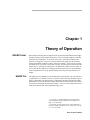
Aluminum
coating
Fiber
100nm
50nm
Aluminum
coating
Sample Surface
Figure 1-1
DISTANCE
CONTROL
MECHANISMS
Fiber-Optic Probe Tip
Tip geometry alone is not enough to produce images. The tip must also be very close to the
sample, typically <10 nm. These small separations are only possible with electronic
position detection and control. Distance control is currently achieved using a shear-force
mechanism. Two such mechanisms exist: light-lever and tuning fork. For these techniques, the tip is attached to a vibrating element which is driven at its resonant frequency.
This vibration is parallel to the surface. As the tip approaches the surface, the vibration
amplitude and phase change. This change in amplitude and phase generates an electrical
signal that is input into the feedback loop.
The Aurora-2 uses the tuning fork mechanism for distance control, as it has the advantage
of producing an electrical signal directly, rather than relying on another device to generate
a signal. This direct connection provides better feedback control, uses much smaller
vibration amplitudes, and does not introduce unwanted light into the sample area.
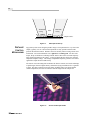
Fiber
Contacts
Tuning fork
Figure 1-2
Aurora-2 Fiber-Optic Probe
THEORY OF OPERATION
1-3
The fiber-optic probe is attached to one prong of a piezoelectric tuning fork. The tip
extends slightly beyond the end of the tuning fork. The tuning fork is vibrated using a
dithering piezoelectric device, which produces a vibrational amplitude at the tip of approximately one nanometer. As the piezoelectric material of the fork vibrates, it produces a
small current. The vibration amplitude of the fiber can then be measured by measuring the
piezoelectric signal from the tuning fork. The current is amplified and input into a lock-in
amplifier. The phase change of the tuning fork signal relative to the driving signal is
measured and used in the feedback loop.
Figure 1-3
MODES OF
OPERATION
Tuning Fork Mechanism
The NSOM instrument is a unique combination of a scanning probe microscope and an
ultra-high resolution optical microscope. Generally both modes—topography and
optical—are used together. However, there may be some situations where topography is
used alone.
The NSOM, used as an optical microscope, can be operated either in tip collection or tip
illumination mode. In tip collection mode, the sample is the light source, and the tip acts
as a way to collect this light. This method is best for samples such as waveguides and laser
diodes.
Tip illumination mode is perhaps the most common NSOM mode. Tip illumination uses
the tip as a “light funnel” to illuminate the sample in a precise, controlled manner. This
mode can be further subdivided into reflection collection, transmission collection, and lithography modes. Reflection collection gathers light that has been reflected from the
sample. It is used for opaque samples, such as semiconductor materials. This method is
not as efficient for gathering light, since the physical position of the tip collector does not
allow it to collect much of the reflected light. Reflection mode might also suffer from
image artifacts created by tip shadowing on the sample surface. Transmission mode is
more commonly used and is more efficient. The collector is placed behind the sample and
collects a majority of the light as it passes through the sample. The drawback to this mode
is that it requires the use of thin, transparent samples.
Aurora-2 User’s Manual
1-4
There are a number of operational techniques in transmission mode. The major techniques
are bright field, fluorescence, polarization, and spectroscopy. These techniques use
different properties of light. Bright field mode is similar to standard optical microscopy in
that the sample is exposed to light from the NSOM probe, and the resulting image is
recorded by detecting all wavelengths, including the source light, on the photomultiplier
tube (PMT). In fluorescence modes, the tip is used to excite the sample, and any resulting
fluorescence is captured and imaged. Polarization mode typically polarizes the incoming
light and looks at how the sample changes that polarization. In spectroscopy techniques,
the signal is the change (either time-scale or wavelength) the sample causes in the exposing
light. Figure 1-4 illustrates the relationships between these operational modes.
Sample Types
Tip 4
Collection
Optical
&
Topography
Waveguides
LED's
Diode lasers
Opaque Samples
Semiconductors
1
Reflection
Tip
Illumination
Transmission
Lithography
Figure 1-4
Bright field
2
3
Fluorescence
Polarization
Spectroscopy
NSOM Operational Modes
Examples of NSOM imaging with the Aurora, using the modes referenced in Figure 1-4,
are included in the following literature.
1. P.J. Moyer, T. Cloninger, J. Gole, and L. Bottomley. Experimental evidence for
molecule-like absorption and emission of porous silicon using near-field and far-field
optical spectroscopy. Phys. Rev. B, 60, No. 7, 4889-4896 (1999).
2. P.F. Barbara, D.M. Adams, and D.B. O’Connor. Characterization of organic thin film
materials with near-field scanning optical microscopy (NSOM). Annu. Rev. Mater. Sci.,
29, 433-469 (1999).
3. A. Naber, H. Kock, and H. Fuchs. High-Resolution Lithography with Near-Field
Optical Microscopy. Scanning Vol. 18 (8), 567-571 (1996).
4. Ch. Lienau, A. Richter, A. Klehr, and T. Elsaesser. Near-Field Scanning Optical Microscopy of Polarization Bistable Laser Diodes. Appl. Phys. Lett. 69, No. 17, 2471-2473
(1996).
CH APTER
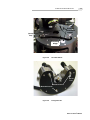
Chapter 2
Aurora-2 Overview & Set-Up
INSTRUMENT
OVERVIEW
The Aurora-2 instrument is a platform for obtaining topographic and optical images. It
offers a wide variety of configuration options, depending on the desired NSOM imaging
mode. The sample is mounted on a scanning stage which is controlled by a three-piezo
scanner arrangement. The fiber-optic probe is mounted on the removable Aurora-2 microscope head and positioned above the sample. Topographic and optical images can be taken
simultaneously.
Probe
Sample Stage
Control
electronics
XYZ
Piezo
Figure 2-1
Topography Feedback Loop
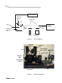
The optical components of the Aurora-2 system are used for taking NSOM data as well as
for focusing the optics and monitoring the probe-sample approach. The rotating mirror (see
Figure 2-2) selects either the reflection or transmission objective. The two “flipper”
mirrors can be manually flipped down to allow the use of the PMT or optional hardware,
such as a photon counter or spectrometer.
Aurora-2 User’s Manual
2-2
.
Laser & coupler
Reflection
objective
lens
Flipper mirrors
Stage
Focusing
lenses
Rotating
mirror
Transmission
objective
lens
CCD
camera
Figure 2-2
{
{
Reflection
objective
Transmission
objective
Photomultiplier
tube (PMT)
Aurora-2 Light Path
Reflection
tower
Camera flipper
mirror (hidden) PMT flipper
mirror
Head
Scanning
stage
&
Optional
Hardware
CCD Camera
PMT
Cam splicer
Figure 2-3
Instrument Components
AURORA-2 OVERVIEW & SET-UP
2-3
AURORA-2 PACKAGE
STANDARD
COMPONENTS
All the components of the basic Aurora-2 configuration are listed below. It is a good idea
to go through this list to be sure that all the items have been received. Shipping errors can
be corrected by contacting Customer Service.
• Instrument stage (base plate with mounted hardware)
• Aurora-2 sensor head
• Electronic Control Unit-Plus (ECU-Plus) with I/O 10 and I/O MOD+ boards
• Aurora Control Unit
• Computer
• Video monitor
• NSOM fiber-optic tips
• Probe installation tool
• Fiber cleaver
• Fiber stripper tool
• Tool kit
• Cables
• NSOM standard sample
• User’s Manual
• Instrument enclosure
• SPMLab software
• SPMLab Software Reference Manual
OPTIONAL
EQUIPMENT
• I/O-U input/output board
• I/O-P photon counter board
• Laser
• Laser coupler
• Daughter board for additional analog-to-digital conversion channels
• Explorer SPM head
• Vibration isolation table
The Explorer SPM head is a popular option, as it uses the same control hardware as the
Aurora-2. The User-Access board (I/O-U) provides access to most of the input and monitor
signals on the ECU-Plus. The photon counter interface board (I/O-P) allows the user to
collect data through a photon counter, which is useful for very low light levels. Contact the
ThermoMicroscopes representative in your area for more information on these options.
Aurora-2 User’s Manual
2-4
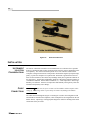
Fiber stripper
Fiber cleaver
Probe installation tool
Figure 2-4
Probe and Fiber Tools
INSTALLATION
INSTRUMENT
LOCATION
CONSIDERATIONS
CABLE
CONNECTIONS
The Aurora-2 should be mounted in an environment that is as vibration-free as possible.
Sources of mechanical and acoustic vibration will decrease the Aurora’s maximum resolution capability. The Aurora-2 should be placed on a its own vibration isolation table.
Computer cooling fans and mouse clicks produce vibration that negatively impacts image
quality, so place the computer on a separate table. Basement or ground floor rooms are
better for the instrument, since multi-story buildings usually have significant vibration on
the upper floors. Temperature and humidity should be controlled to maintain constant environmental conditions. Normal indoor conditions, i.e., “room temperature” and average
humidity, are sufficient. Extremes of temperature and humidity will negatively affect the
instrument and possibly cause damage.
Make sure the power is OFF to all the modules and the computer while
setting up. Connecting cables to powered-up electronics may damage the modules.
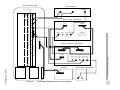
CAUTION
The cable connection diagrams (Figure 2-5 and Figure 2-6) show the configuration with
and without an external lock-in amplifier (a lock-in amplifier is also integrated into the I/O
MOD+ board). A photocopy of the appropriate diagram is useful for checking off the cable
connections as they are made.
AURORA-2 OVERVIEW & SET-UP
POWERING UP
THE SYSTEM
2-5
WARNING
To prevent serious injury, make sure the cover is on the laser coupler
before turning the laser on. Follow all safety warnings when powering up and using the
laser.
Make sure the PMT voltage is turned all the way down (to the counterclockwise limit) before powering up the components.
CAUTION
Once all the connections are made, the components can be powered up. First turn on the
ECU-Plus, then the computer and the video monitor. (The ECU-Plus should always be
turned on before the computer so that the ECU interface is recognized and initialized.) The
laser is powered up separately. Power is automatically applied to the Aurora Control Unit
when the ECU-Plus is powered up.
Aurora-2 User’s Manual
Aurora-2 Stage (Rear Panel)
ECU-Plus (Rear panel)
(Optional)
CABLE 1
DRIVE
OUT 1
A
DRIVE
OUT 2
B
BNC 1
BNC 2
BNC 3
CABLE 2
BNC 4
SIGNAL
IN 1
IN A
SIGNAL
IN 2
IN B
STAGE
OUT 1
OUT 2
OUT 3
STAGE 2
CPU
Aurora-2 Control Unit (Rear panel)
OUT 4
SPARE
MODULE
TO STAGE
EFM
DRIVE
TO ECU
TO STAGE
MOD
IN
POWER
Computer
NSOM MOD
IN
OUT
Video Monitor (Rear Panel)
DSP
IN
Figure 2-5
Aurora-2 Wiring Diagram
NSOM VIDEO
OUT
OUT
OUT
2-6
-P
0
-1
I/O +
D
O
-M
I/O
-U
I/O
I/O
ACU
ECU-Plus (Rear panel)
Lock-In Amplifier
-P
0
-1
I/O +
D
O
-M
I/O
-U
I/O
I/O
INPUT A
OSCILLATOR OUT
or SINE OUT
X
DRIVE
OUT 1
A
DRIVE
OUT 2
B
Aurora-2 Stage (Rear Panel)
SIGNAL
IN 1
IN A
ACU
CABLE 1
SIGNAL
IN 2
IN B
OUT 1
STAGE
BNC 1
BNC 2
BNC 3
CABLE 2
BNC 4
OUT 2
OUT 3
STAGE 2
CPU
OUT 4
Aurora-2 Control Unit (Rear panel)
SPARE
MODULE
EFM
DRIVE
TO STAGE
TO ECU
TO STAGE
NSOM
IN
MOD
OUT
NSOM VIDEO
OUT
OUT
POWER
Computer
Video Monitor (Rear Panel)
IN
Figure 2-6
Aurora-2 Wiring Diagram for External Lock-in Amplifier
OUT
2-7
Aurora-2 User’s Manual
DSP
AURORA-2 OVERVIEW & SET-UP
MOD
IN
2-8
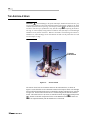
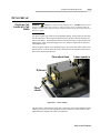
THE AURORA-2 HEAD
CAUTION
To avoid damage to the probe and sample, handle the head with care, paying particular attention to the probe and probe mount on the bottom. Whenever the head
is removed from the microscope stage, use the Tip Up button
on the Data Acquisition
tool bar to raise the tip a safe distance away from the sample. When placing the head on
the stage, or when carefully setting it down on a table or other flat surface, turn the Z-height
thumbscrews one full turn clockwise. Whenever the head is lowered using the Z motor or
thumbscrews, watch the image on the video monitor to make sure the probe does not crash
into the sample or stage.
Z motor
Z-height
thumb screws
Light
Probe
Figure 2-7
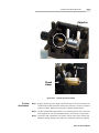
Aurora-2 Head
The Aurora-2 head rests on a kinematic mount on the instrument base, as shown in
Figure 2-8 (note that there is also a kinematic mount for the Explorer head). The Z-height
between the probe and the sample stage is controlled by the three Z-height screws, as shown
in Figure 2-9. On the bottom of each screw is a ball bearing that fits into the kinematic
mount. The motorized screw (Z motor) is controlled with the Tip Up
and Tip Down
buttons on the Data Acquisition tool bar in the SPMLab software. The other two
screws are adjusted manually with the thumbscrews on the head.
AURORA-2 OVERVIEW & SET-UP
2-9
Reflection
objective
Aurora-2
kinematic
mount
(mount
first)
Scanning
stage
Figure 2-8
Kinematic Mount
(mount
first)
Manual screws
Motorized screw
Figure 2-9
Z-Height Screws
Aurora-2 User’s Manual
2-10
PLACING THE
HEAD ON THE
STAGE
Step 1
Turn the Z-height thumbscrews one full turn clockwise.
Step 2
Connect the data cable to the female connector on the head.
Step 3
Hold the head in your left hand, and position it over the stage, being careful not to
hit the reflection objective.
CAUTION
To avoid damaging the piezo scanners, be careful not to touch the stage
with the head.
Step 4
Check to see that there is sufficient clearance between the head and the scanning
stage before lowering the head all the way onto the mount. If necessary, adjust the
thumbscrews so the head does not end up resting on the stage instead of the
kinematic mount.
Step 5
Lower the head slowly onto the kinematic mount, tilting it slightly away from you
so the manual Z-height screw opposite you lowers into the mount first, as shown
in Figure 2-10.
Figure 2-10
Placing the Head on the Stage
Step 6
Lower the head onto the stage so the other two screws come to rest in the mount.
Step 7
If a probe is mounted on the head, tape the fiber-optic cable to the Z motor
enclosure on the head, as shown below in Figure 2-15 on page 14 under
“Installing a Probe.”
AURORA-2 OVERVIEW & SET-UP
REMOVING THE
HEAD
2-11
Step 1
Click the Tip Up button
on the Data Acquisition tool bar to raise the tip a
safe distance away from the sample.
Step 2
Remove the head by first tilting it slightly away from you, pivoting it on the
kinematic mounting, then lifting it safely off the stage.
Step 3
Set the head down on a soft, flat surface, making sure there is no obstruction that
would strike the probe.
MOUNTING THE SAMPLE ON THE STAGE
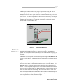
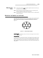
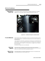
The sample included with the instrument was made by coating a surface with latex spheres
approximately 450 nm in diameter, then depositing aluminum onto the surface. The
spheres are then removed, leaving the coating on the interstitial areas, as shown in
Figure 2-11.
Figure 2-11
Standard Sample Example
To avoid damage to the piezo scanners, do not apply more force than necessary to the scanning stage.
CAUTION
To mount the sample, you must remove the head. The sample slide can simply be scotchtaped to the stage. A piece of tape over each corner will hold the sample in place during
the scan. This technique is the most common one for mounting samples on the Aurora-2
stage. Alternatively, small amounts of immersion oil can be used to hold the sample to the
scanner plate.
Aurora-2 User’s Manual
2-12
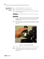
INSTALLING A PROBE
CAUTION
Step 1
Handle the probe with care, as it can be easily damaged.
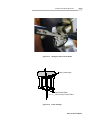
To grasp the probe with the probe installation tool, position the tool over the probe
and fit the two “teeth” into the corresponding gaps on either side of the probe
cartridge, as shown in Figure 2-12.
Figure 2-12
Grasping the Probe with the Probe Tool
Step 2
Press down firmly into the foam lining of the probe box until the tool snaps into
place.
Step 3
Carefully pull the tape off the optical fiber so the probe can be removed from the
box. Unroll the fiber, taking care not to touch the tuning fork or put any strain on
the fiber.
Step 4
Slide the probe into the holder in the head by sliding it under the clips, as shown
in Figure 2-13.
Step 5
Make sure the three clips make contact with the three metal contact pads on the
probe, as shown in Figure 2-14. If necessary, use both thumbs to gently push the
probe all the way into place, while cradling the head with both hands.
AURORA-2 OVERVIEW & SET-UP
Figure 2-13
2-13
Sliding the Probe into the Holder
Probe Contact Clips
Gold Contact Pads
Piezo Tuning Fork and Fiber
Figure 2-14
Probe Cartridge
Aurora-2 User’s Manual
2-14
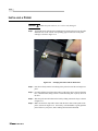
Step 6
Raise the thumbscrews located on the front of the head by turning them clockwise
one full turn. This will keep the tip from hitting the stage when the head is placed
on the stage.
Step 7
Carefully place the head on the stage, and plug the data cable into the head, as
described above on page 2-10.
Step 8
Tape the fiber to the Z motor enclosure on the head, as shown in Figure 2-15. This
takes strain off the fiber and helps prevent separation from the probe.
.
Figure 2-15
Step 9
Fiber Taped to the Aurora-2 Head
Use the fiber stripper tool to strip away about 25mm of the polymer buffer off the
end of the tip fiber. Note that once stripped, the fiber is very brittle.
Step 10 Use the optical fiber cleaver from the tool kit to cleave the end of the tip fiber:
(a) Open the jaws of the cleaver, and seat the fiber into the notch in the lower jaw.
(b) Insert the fiber until the stripped portion on the end aligns with the 16 mm mark.
(c) Press the scoring bar down on the fiber. Take care not to break the fiber.
(d) Gently flex the tongue of the cleaver down until the fiber cleaves. Take care not
to touch the tip.
Step 11 Carefully insert the fiber into one end of the cam splicer. Gently roll or twist the
fiber as it is inserted to help it enter. Insert about 15mm into the splicer. Leave
the coupler open, with the lock arms up.
Step 12 Gently seat the fiber into the fiber holder on the end of the cam splicer assembly.
AURORA-2 OVERVIEW & SET-UP
2-15
Lock arms
Figure 2-16
Cam Splicer
Fiber Holders
Figure 2-17
Cam Splicer Assembly
Aurora-2 User’s Manual
2-16
AURORA CONTROL UNIT
CAUTION
Keep the PMT Voltage on the Aurora Control Unit set to 0, unless the PMT
is shielded from all sources of light (except the laser during NSOM imaging). Exposure to
light can damage the PMT. The voltage should only be turned up when carefully following
the procedures in Chapter 4.
AFM
PMT VOLTAGE
CONTROL
LIGHT
BRIGHTNESS
FEEDBACK
NSOM
PMT
VOLTAGE
PMT
OUTPUT
ON
LIGHT
OFF
AURORA CONTROL UNIT
Figure 2-18
Aurora Control Unit
Power is applied to the Aurora Control Unit (ACU) when the ECU-Plus is powered up.
Failure to observe all CAUTION notices regarding the controls on the ACU may result in
damage to the PMT and probe tip.
The light controls refer to the light on the Aurora-2 head that illuminates the sample area.
This light is only used in procedures that involve the video monitor and should not be on
during NSOM scanning or any time the PMT voltage is turned up.
Note that the Feedback switch is not connected in the current configuration.
AURORA-2 OVERVIEW & SET-UP
2-17
OPTICS CONTROLS
TRANSMISSION
OBJECTIVE
The transmission objective, positioned directly beneath the sample stage, is manually
adjusted in X, Y, and Z (focus) with the translation knobs shown in Figure 2-19.
X
Y
Z (focus)
Figure 2-19
FLIPPER MIRRORS
Transmission Objective Translation Knobs
The two flipper mirrors can be flipped up or down to select the desired path of the beam
leaving the reflection tower. The beam can be directed to the CCD camera, the PMT, or to
optional hardware.
Coarse adjustment of each mirror is performed by loosening the screw underneath the supporting column. Use the yoke supplied with the Aurora-2 to hold the mirror temporarily in
place while the position is adjusted. Once the position is set, tighten the screw under the
base of the column.
The X and Y fine-adjust screws are on the mount.
ROTATING
MIRROR
REFLECTION
OBJECTIVE
The rotating mirror is controlled by a knob on the front of the stage, as shown in
Figure 2-20. The knob has two positions: the counter-clockwise limit selects the reflection
objective; the clockwise limit selects the transmission objective.
The reflection objective is focused by manual rotation of the lens. The manual tilt and
swivel translation knobs are shown in Figure 2-20.
Aurora-2 User’s Manual
2-18
Tilt
Focus
Swivel
Rotating
mirror
selector
Figure 2-20
Reflection Tower Controls
AURORA-2 OVERVIEW & SET-UP
2-19
OPTICS SET-UP
COUPLING THE
LASER INTO THE
FIBER
WARNING
Always use caution when operating the laser. NEVER look directly into
the laser aperture, fiber end, or probe tip. This can cause severe eye damage and even
blindness. Follow all the safety precautions and instructions that pertain to use of the laser
and laser coupler.
Two pieces of fiber-optic cable are used in NSOM scanning: the laser fiber (the piece that
runs from the laser to the cam splicer) and the tip fiber (the piece that runs from the cam
splicer to the probe). The instructions in this section describe how to couple the laser into
the laser fiber. These instructions apply to the laser and laser coupler sold as options by
ThermoMicroscopes.
The laser coupler consists of two translation stages: one for the fiber chuck, which can be
moved in the X, Y, and Z (focus) directions, and one for the fine adjustment lens located
between the objective and the laser.
Laser aperture
Fine adjust lens
Y
Y
Z (focus)
X
X
Fiber
chuck
Figure 2-21
Laser Coupler
The fiber chuck is adjusted when a new fiber is inserted or when a large adjustment of the
coupling is necessary. The fine adjustment (closest to the laser) is used to make a small
adjustment to the coupling after it has been optimized.
Aurora-2 User’s Manual
2-20
The procedures for inserting a fiber into the coupler and coarse adjustment are generally
performed only once, by the service engineer when the instrument is installed. However,
these instructions are included so the user can adjust the coupling to achieve maximum
power transfer into the fiber, or in the event that a new fiber is used. The fine adjustment
of the coupling is performed more often.
To better understand the fiber coupler, you can remove the cover, as instructed in the section
below, and follow along with the descriptions of the various components.
WARNING
Make sure the laser is turned off when the cover to the laser coupler is
removed, or wear the appropriate laser safety goggles. NEVER look directly into the fiber
tip or laser aperture! Severe eye damage or blindness could result.
INSERTING A FIBER IN
THE COUPLER
Step 1
Remove the cover from the coupler. You will see that the fiber is held by a brass
coupler chuck. The chuck is held in position by a chuck clamp. The clamp can
be translated in the X, Y, and Z to position the fiber in the laser beam.
Step 2
When it is time to use a new fiber, remove the coupler chuck from its clamp by
unscrewing the lock collar on the end of the coupler and removing the old fiber.
Step 3
Feed the new fiber through the chuck far enough so you can strip and cleave the
end of the fiber.
Step 4
Carefully strip about 10mm of the polymer buffer off the fiber.
Step 5
Cleave the fiber at about 3-5mm, and pull the new cable back into the chuck, with
about 5mm of fiber extending from the lock collar. (More detailed instructions on
how to cleave the fiber are given on page 2-22.)
Step 6
Replace the chuck in the chuck clamp, with the cleaved end of the fiber facing the
laser objective lens. The distance between the cleaved end of the fiber and the
objective lens should be approximately 3mm.
Step 7
Tighten the chuck clamp to hold the chuck securely.
Step 8
Replace the cover.
Step 9
Temporarily secure the other end of the fiber in a way that will not pose a risk of
laser light exposure to anyone’s eyes. Tape it to the Aurora-2 base plate or gently
seat it into the fiber holder on the end of the cam splicer assembly.
AURORA-2 OVERVIEW & SET-UP
2-21
Objective
Chuck
Chuck
clamp
Figure 2-22
COARSE
ADJUSTMENT
Coupler Chuck and Clamp
Step 1
Begin by turning the power adjust control on the laser to its lowest setting (to the
counterclockwise limit), then turn on the power to the laser. The laser is operated
on the low setting. High power settings may introduce unwanted noise.
Step 2
The fiber end should be approximately 3 mm from the objective lens. This is the
focal length for the lens. The maximum intensity will be at this 3 mm position.
Step 3
Aim the free end of the fiber at a flat surface, such as a table, wall, or index card.
Watch the intensity change as the coupler X-Y translation controls are adjusted.
Aurora-2 User’s Manual
2-22
FINE ADJUSTMENT
COUPLING THE
LASER LIGHT INTO
THE PROBE
Step 4
The Z axis—the fiber focus ring—may need to be slightly adjusted for maximum
power. The focus is correct when small changes in X and Y translation produce
large changes in intensity. The fiber is out of the lens focal region when large X
and Y translation produces little change in light intensity. After adjusting the Z
axis, it is usually necessary to re-adjust the X and Y translation.
Step 5
Adjust the X axis for maximum light intensity, then adjust the Y axis. Go back
and re-check the X axis, then re-check Y. Go back to Step 4 if the Z axis needs
further optimization.
Use the X-Y fine adjustment closest to the laser to optimize the coupling.
NEVER look directly into the fiber tip or laser aperture! Severe eye
damage or blindness could result.
WARNING
Coupling the laser light into the probe is a procedure that is performed frequently. It can
be repeated any time it seems the intensity at the tip could be improved.
The tip fiber should be stripped and temporarily installed in the cam splicer, as described
on page 2-14.
CAUTION
Do not follow this procedure when the tip is in feedback.
Step 1
Use the fiber stripper tool to strip away about 25mm of the polymer buffer off the
end of the laser fiber. Note that once stripped, the fiber is very brittle.
Step 2
Use the optical fiber cleaver from the tool kit to cleave the end of the laser fiber
(you may also want to refer to the documentation supplied with the fiber cleaver):
(a) Open the jaws of the cleaver, and seat the fiber into the notch in the lower jaw.
(b) Insert the fiber until the stripped portion on the end aligns with the 16 mm mark.
(c) Press the scoring bar down on the fiber. Take care not to break the fiber.
(d) Gently flex the tongue of the cleaver down until the fiber cleaves. Take care not
to touch the tip.
Step 3
Carefully insert the laser fiber into the cam splicer at the opposite end from the tip
fiber. To help the laser fiber enter, gently roll or twist it as it is inserted . Insert
the laser fiber far enough to touch the tip fiber. Pushing on one fiber should move
the other fiber.
Step 4
Put the splicer arms in the locked (down) position.
Step 5
Gently seat the laser fiber into the fiber holder on the end of the cam splicer
assembly.
Step 6
Check to see that laser light is coupled into the tip fibertip fiber. The laser light
may not be visible at the tip, but if the room lights are turned off, the tip fiber
should be glowing. If there is no light visible in the tip fiber, repeat Steps 2-5.
AURORA-2 OVERVIEW & SET-UP
2-23
Note that once the tip has been coupled to the laser, thermal expansion of the tip will take
place for the next few minutes. It is a good idea to wait approximately 15 to 20 minutes
before attempting a scan, to allow the tip to reach thermal equilibrium.
OPTICAL TRAIN
ALIGNMENT
The Aurora-2’s optical train has been adjusted at the factory, and the service representative
who installed the system has made final adjustment corrections. However, the user should
be able to make adjustments to the optical path if necessary.
The objective of this procedure is to have the center of the optical beam pass through the
center of each optical element in its path. This means that the image beam should be
centered on both the transmission and reflection lenses, the beam mirrors, the prisms, the
focusing lenses, and the CCD camera and PMT detector faces (see Figure 2-2 on page 2).
This is essentially the same goal as in any optical system, and the procedures for achieving
this goal are similar.
Precise optical adjustment is critical for NSOM imaging and any advanced techniques.
Because the tip emits little light, the optical path must be accurately focused to collect the
maximum amount of light with the detector. If the detector signal strength is very low,
make sure that none of the beam is being lost along the path and that the beam is focused
on the detector.
For this procedure, you will need a small piece of paper to use as a “beam finder.” The back
of a business card or index card works well for this.
CAUTION
Keep the PMT Voltage on the Aurora Control Unit set to 0, unless the PMT
is shielded from all sources of light (except the laser during NSOM imaging). Exposure to
light can damage the PMT. The voltage should only be turned up when carefully following
the procedures in Chapter 4.
Step 1
Set up the Aurora-2 as described in the above procedures in this chapter. It is
assumed that the user is familiar with removing and replacing the head and
mounting a sample.
Step 2
If the system is not powered up, first turn on the ECU-Plus, then the computer and
the video monitor. (The ECU-Plus should always be turned on before the
computer so that the ECU interface is recognized and initialized.)
Step 3
Open the SPMLab software, and enter the Data Acquisition module.
Step 4
Turn on the light on the Aurora-2 head with the switch on the Aurora Control Unit.
This light illuminates the sample during tip positioning and focusing.
Step 5
Remove the head from the stage, if necessary.
Step 6
Mount the ThermoMicroscopes NSOM standard sample on the stage. The easiest
way to do this is by using a few small pieces of tape at the corners of the sample.
Or, you can put a small drop of immersion oil underneath the sample.
Step 7
Turn the Z-height thumbscrews on the head one full turn clockwise, and carefully
place the Aurora-2 head on the stage, lowering the head slowly to make sure the
tip does not touch the sample when it comes to rest in the kinematic mount. The
tip should now appear in the video monitor.
Aurora-2 User’s Manual
2-24
The tip may be difficult to find in the reflection optics if it is too far from the
sample. Check the tip-sample area by eye to get an idea of the distance, and use
the manual thumbscrews to lower the head, if necessary, being careful not to
crash the tip into the sample.
Step 8
Use the video monitor to focus the image in both transmission and reflection
modes. Use the rotating mirror to switch back and forth between these images.
The tip should appear in the middle of the monitor. Use the appropriate focus
controls for the transmission and reflection objectives.
Step 9
Rotate the mirror to reflection mode, and focus the optics on the sample. This
image should be the more easily recognizable of the two.
Step 10 Click on the Tip Down button
on the Data Acquisition tool bar to lower the
tip until it is within a few millimeters of the stage, as seen on the video monitor.
Step 11 Focus the reflection optics on the tip.
Step 12 Rotate the mirror to transmission mode, and focus the optics on the sample.
Step 13 Once both transmission and reflection mode images are focused, look at the image
on the video monitor. The image should fill the monitor, and no edges should be
visible. If the edges can be seen, use the X and Y fine adjust screws on the camera
path flipper mirror mount to center the image. Be sure to check both transmission
and reflection images after making an adjustment.
Step 14 Flip the mirror to the down position when finished centering the image.
Step 15 Using the “beam finder,” find the beam leaving the reflection tower. Make sure
the beam is hitting the PMT path mirror. This mirror’s coarse position can be
adjusted by loosening the screw underneath the supporting column. Use the yoke
supplied with the Aurora-2 to hold the mirror temporarily in place while the
position is adjusted. Once the position is set, tighten the screw under the base of
the column.
Step 16 Trace the beam from the path mirror to the focusing lens. Make sure the beam
intersects the middle of the lens. If needed, the lens position can be adjusted the
same way the mirror’s position was.
Step 17 Make sure the beam is focused on the center of the PMT’s detector window. Slide
the lens back and forth so the beam is focused as nearly as possible on the tube
aperture. Or, you can unscrew the PMT from its support bracket (4 screws).
Once adjusted, the instrument should not require major optical path alignment. The instrument is now ready to take a scan.
CH APTER
Chapter 3
Taking a Topographic Image
PROCEDURE
OVERVIEW
NSOM combines both topography and optical imaging. It is common to take a topographic
image first to allow the user to set up the scan parameters and potentially identify features
of interest on the sample. Then the laser is coupled into the tip, and a combined topographic
and optical scan is taken.
Before taking an NSOM image, it is essential to master taking a topographic image, which
is nearly identical to non-contact Atomic Force Microscopy (AFM) techniques. Topographic scanning requires learning the techniques for bringing the tip into feedback. When
the tip is in feedback, it can track the topography of the sample, thus it is in the near-field
range of the sample, which is necessary for NSOM imaging.
Chapters 3 and 4 cover this two-part technique for taking a scan of the standard sample
included with the instrument. The combined scan techniques described below will be applicable to any sample.
The instructions in this chapter assume that the Aurora-2 has already been set-up as
described in Chapter 2. All components should be powered up, and the Data Acquisition
module of the SPMLab software should be open.
Aurora-2 User’s Manual
3-2
APPROACHING THE SAMPLE
CAUTION
Be careful when lowering the tip not to crash it into the sample surface.
Feedback refers to the attenuation of the tip’s oscillation amplitude. When the tip is in
feedback at the sample surface, the sample topography can be tracked and a topographic
image taken. This also means that the tip is in the near-field range, enabling NSOM
imaging. A technique known as “false feedback” will be used to bring the tip into the near
field. This allows for a gentle yet efficient approach, whereas using the Z-motor to
approach the sample runs the risk of breaking the tip and is usually very slow.
FINDING THE
RESONANT DRIVE
FREQUENCY
For each probe, it is necessary to set the drive frequency at the resonant frequency of the
tuning fork. The objective is to maximize the magnitude of the tuning fork vibration by
adjusting the driving frequency control.
For the following procedure, refer to the “Non Contact Operation” section in Chapter 2 of
the SPMLab Software Reference Manual. When the SPMLab software is configured for
the Aurora-2, the Non Contact window is automatically open, with the Active mode
checked, upon entering the Data Acquisition mode.
Step 1
Select “Internal Sensor, Feedback” from the drop-down signal source list to the
right of the upper oscilloscope.
Step 2
Select Amplitude from the Mode group box in the Non Contact window.
Step 3
In the Non Contact window, enter the following starting parameters:
Amplitude = .1 V
(drive amplitude)
Input Gain = 8.
(input gain of the I/O MOD+ board)
Step 4
In the Signal window, select SCOPE mode.
Step 5
From the Range drop-down list, select the frequency range that is closest to 90100 kHz, which is typical for the tuning fork.
Step 6
In the Non Contact window, select SPECTRUM to run a frequency sweep.
Step 7
Zoom in on the peak so that the frequency window is 2 kHz (or less) wide.
Step 8
Make sure the peak is not cut off. The maximum voltage range of this window is
10 V. If the peak is cut off, reduce the Amplitude. Ideally, the peak will sit at
around 5 V, which corresponds to about -30nA on the internal sensor signal. Fine
tuning will be done later.
Step 9
Click on the peak to select the drive frequency, which will then appear in the
DRIVE FREQUENCY field. See Figure 3-1.
TAKING A TOPOGRAPHIC IMAGE
Figure 3-1
3-3
Selecting the Drive Frequency
Step 10 Select PHASE from the Mode group box in the Non Contact window, and watch
the internal sensor signal.
Step 11 Click on the AUTO PHASE button in the Non Contact window. The internal sensor
signal should go to 0.
Step 12 Click on the +90 button three times (for a total of 270 degrees) to find the phase
that shows the most negative value for the internal sensor signal.
Step 13 Fine tune the Non Contact controls using the following guidelines:
The aim to have the drive amplitude be as low as possible while keeping the
internal sensor signal at approximately the same value and the RMS noise (displayed in blue in the Signal window) less than 0.1.
Reducing the drive amplitude will cause the internal sensor signal to increase
(move closer to 0). Increasing the gain will bring the internal sensor signal down
(more negative, i.e., further from 0). However, increasing the gain will proportionally increase the RMS noise.
Step 14 Once the Non Contact controls have been fine-tuned, minimize the Non Contact
window. To adjust these settings, the tip must be out of feedback. These settings
will be saved when you exit the SPMLab software.
MOVING THE TIP
INTO FEEDBACK
Step 1
Set the rotating mirror to reflection mode.
Step 2
Use the thumbscrews to lower the head. Bring the tip within a few millimeters of
the surface.
Step 3
Lower the set point below the current sensor signal level. For example, if the
sensor signal level is -30 nA, lower the setpoint to -50 or -60 nA.
Step 4
Select “Z-Piezo” from the drop down signal list to the right of the lower
oscilloscope to monitor the z-piezo voltage.
Aurora-2 User’s Manual
3-4
Do not leave the z-piezo in its fully retracted position (-220 V), as this
causes it to wear out very quickly.
CAUTION
Step 5
Click the TIP APPROACH button on the Acquisition Control Panel. The z-piezo
should fully retract, as shown by a z-piezo voltage of -220 V. The tip is now in
“false feedback.”
Step 6
Watch the video monitor while lowering the tip with one of the two manual
thumbscrews. Bring the tip as close to the sample surface as possible without
crashing the tip.
It may be useful to monitor the tip both with the light on and off. When the light
is off, and the laser is coupled into the probe fiber, the tip appears as a bright spot
and will be reflected on the sample’s surface. When the light is on, a dark image
of the tip and the length of the fiber is visible, and the image will be reflected on
the sample’s surface.
Step 7
Set the P-I-D settings to:
P≈1
I ≈ 0.04
D=0
The P-I-D settings should be low (the Integral gain in particular) so the tip
doesn’t jump as it approaches the sample.
Step 8
Click on the SET button to the right of the internal sensor signal. The current
internal sensor signal value (on the horizontal line at the middle of the window)
can now be read clearly.
Step 9
Enter the internal sensor signal value (or a slightly lower value, to be safe) in the
SET POINT field.
Step 10 Click the up arrow next to the SET POINT field to raise the value in small
increments until the z-piezo moves.
Never turn the light on or off when the tip is in feedback at the surface. A
voltage spike could cause a tip break.
CAUTION
CAUTION
Do not power down the electronics while the tip is in feedback at the sur-
face.
Step 11 Monitor the z-piezo voltage. If the tip was within scanner range of the surface, the
z-piezo voltage should steadily rise and stabilize at some arbitrary value,
somewhere between -220 and 220 V, dependant on how far the tip was from the
sample surface. The tip is now in feedback at the surface (“true feedback”), and
you can skip to the next section to take a topography scan.
TAKING A TOPOGRAPHIC IMAGE
3-5
Step 12 If the z-piezo signal reaches full deflection, 220 V, the tip was not within scanner
range of the surface. Retract the scanner with the z-piezo by setting the setpoint
significantly below the sensor signal value (i.e., -50 or -60 nA). Watch the z-piezo
signal voltage, and make sure it drops to -220 V.
Step 13 Watch the video monitor image while using the thumbscrews or the z motor (Tip
Down button
) to carefully lower the tip. Be very careful not to crash the
tip into the surface.
Step 14 Enter the internal sensor signal value (or a slightly lower value, to be safe) in the
SET POINT field.
Step 15 Click the up arrow next to the SET POINT field to raise the setpoint above the
current sensor signal value again. Monitor the z-piezo voltage as the tip nears the
surface. Again, the z-piezo voltage should stabilize somewhere between -220 and
220 V.
Step 16 If the piezo reaches full deflection, repeat Steps 12-15 until the z-piezo voltage
stabilizes within the voltage range.
TAKING A TOPOGRAPHY SCAN
To avoid crashing the tip and damaging both the tip and sample, the
P-I-D settings must be set properly.
CAUTION
Once the tip is in feedback with the surface, the P-I-D settings are adjusted to optimize the
scan. These settings tune the distance control feedback circuit to respond quickly and accurately to changes in surface topography. This gives the best topographic imaging.
OPTIMIZING THE
P-I-D SETTINGS
Step 1
Set the Integral gain between 0.08 and 0.30. This range might change depending
on the sample and the specific tip.
Step 2
Click the LINE scan option in the upper right of the Signal window. This scan
mode lets the user evaluate the changes to the internal sensor and topography
signals as the scan rate, setpoint, and P-I-D settings are adjusted. Line scan mode
scans over the same line on the sample and displays three overlaid profiles, each
displayed in a different color. This display allows the user to adjust the scan
parameters to get a stable, repeatable scan.
Step 3
Select “Internal Sensor, Feedback” (upper oscilloscope) and “Topography” (lower
oscilloscope) from the drop-down signal source lists in the Signal window.
Step 4
Monitor the signal while you perform a line scan. If the Integral gain setting is too
high, you will notice oscillations in one or both signals.
Step 5
Set the Proportional gain to 1. If the system oscillates, lower the Proportional gain
until the oscillation stops, then raise it slowly. Usually the Proportional gain is set
between 0.5 and 1.
Step 6
Make sure the Derivative gain is set to 0 (this setting is generally not used).
Aurora-2 User’s Manual
3-6
Step 7
Set the scan rate to about 1/2 the scan range, e.g., if the range is set to 20 µm, the
scan rate would be about 10 µm/s. Τhe scan rate can be a very important
parameter in obtaining a stable signal. If the sample has high topographic
features, and a stable signal cannot be obtained by lowering the P-I-D settings,
reduce the scan rate.
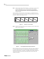
If the line scan has a “sawtooth” shape, as shown in Figure 3-2, with the left slope very
steep and the right slope relatively flat, it is typically an indication that the tip is too far from
the surface, or that the P-I-D settings are too low.
Figure 3-2
Step 8
“Sawtooth” Line Scan Shape
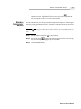
When the P-I-D settings and set point are set properly, you will see a quiet, stable
signal, as shown in Figure 3-3.
Figure 3-3
Properly Adjusted P-I-D Settings and Set Point
When a scan begins, the line scan of the internal sensor signal will no longer be displayed.
To view the internal sensor signal, set the Signal window to SCOPE mode, and open an
internal sensor signal window: select SETUP ⇒ ACQUIRE, and from the Data Channels list,
check the Fwd checkbox for the Internal Sensor channel (this can not be done when
scanning is in progress).
TAKING A TOPOGRAPHIC IMAGE
Step 9
ENDING A
TOPOGRAPHY
SESSION
3-7
Take a scan of the sample by clicking the Instant Scan button
on the Data
Acquisition tool bar. Adjustments to the P-I-D settings can be made while the
scan is being taken. There is no need to restart the scan.
To take an NSOM scan, leave the tip in feedback and proceed to Chapter 4, as all the signal
parameters are already adjusted correctly. Note that it is important to attain some proficiency in taking topographic scans before taking an NSOM scan.
CAUTION
Do not power down the electronics while the tip is in feedback at the sur-
face.
Step 1
Click the Instant Scan button
to stop scanning.
Step 2
Click on the Tip Up
button on the Data Acquisition tool bar to raise the tip
away from the sample, bringing the tip out of feedback.
Step 3
Exit the SPMLab software.
Aurora-2 User’s Manual
3-8
CH APTER
Chapter 4
Taking an NSOM Scan
Before following this NSOM scanning procedure, the Aurora-2 should be set up as
described in Chapter 2, and you should have taken a topography scan following the
procedure in Chapter 3. In order to take an NSOM scan, it is important to attain some proficiency in taking topographic scans.
CAUTION
The Photomultiplier Tube (PMT) can be damaged by repeated exposure
to high light levels with the voltage supplied to the tube. More importantly, repeated exposure will degrade the PMT’s sensitivity over time, resulting in degraded performance. It is
a good practice to protect the PMT from high light levels, which helps ensure long detector
lifetime. When concluding an NSOM session, wait 10-15 seconds before exposing the PMT
to light. In general, whenever the voltage is supplied to the tube, the PMT should be in a
dark environment.
CHECKING FEEDBACK PARAMETERS
These parameters should still be set correctly from the topographic scan. However, as the
tip heats and expands, some adjustments might have to be made to the P-I-D settings. Also,
it is a good idea to recheck the tuning fork resonance frequency. Following the guidelines
in Chapter 3, adjust the P-I-D settings for the best signal. Recheck these settings immediately before beginning the scan.
Aurora-2 User’s Manual
4-2
APPROACHING THE SAMPLE AND TAKING A SCAN
Refer to Chapter 3, observing all Warning and Caution statements, when following this procedure.
Step 1
Locate the tip with the transmission and reflection objectives.
Step 2
Bring the tip into feedback, if it is not already, following the procedure under
“Moving the Tip into Feedback,” on pg. 3-3.
Step 3
The z piezo voltage should be around 0.
Step 4
Pull the z piezo back by typing in a set-point value that is more negative than the
internal sensor signal. E.g., if the internal sensor signal is -30 nA, type in -64 nA.
The piezo will retract. This is done so the tip doesn’t break when you flip the
mirror.
Step 5
Make any final necessary adjustments to the transmission objective. The image
should be in focus and in the middle of the monitor.
Step 6
Flip the camera path mirror down, to open the PMT path.
Step 7
Close the instrument enclosure and, if possible, dim or turn off the room lights.
Step 8
Turn off the Aurora-2 light.
CAUTION
Step 9
The light on the Aurora-2 must be off to prevent damage to the PMT.
Select SETUP ⇒ ACQUIRE, and from the Data Channels list check the FWD
checkbox for the NSOM channel.
Step 10 Bring the tip back into “true feedback,” i.e., at the sample surface, as described in
Steps 7-16 under “Moving the Tip into Feedback,” on pg. 3-3. The P-I-D settings
should be low (the Integral gain in particular) so the tip doesn’t jump as it
approaches the sample. Be sure to observe all the Warning and Caution
statements!
Step 11 Increase the P-I-D settings to improve the topography response, following the
procedure under “Optimizing the P-I-D Settings,” on pg. 3-5.
Step 12 Click the SCOPE option in the upper right of the Signal window, and choose
“NSOM” from the drop-down signal source list to the right of the upper
oscilloscope. The signal should read 0, both on the oscilloscope and the Aurora
Control Unit.
Step 13 Slowly turn up the PMT voltage on the Aurora Control Unit. The PMT will
typically “turn on” at around 230 V. Watch the PMT signal, and make sure there
is a signal response as the PMT voltage is increased. Aim for a signal of about
200mV. Increasing voltage increases the signal strength, but it also increases the
noise level within the signal.
Step 14 Perform a line scan by clicking the LINE option in the Signal window.
Step 15 Adjust the set point and the P-I-D settings until you get repeatable line scans, as
shown in Figure 4-1.
TAKING AN NSOM SCAN
Figure 4-1
4-3
Optimized Line Scans
CAUTION
Lower the PMT voltage immediately if you notice a sudden, dramatic increase of the NSOM signal (indicating a tip break). Exposure to these high light levels will
permanently damage the PMT.
Step 16 Begin a scan by clicking the Instant Scan button
on the Data Acquisition tool
bar. Adjustments to the P-I-D settings and set point can be made while the scan is
being taken. There is no need to restart the scan.
During the scan, you can keep the oscilloscope in LINE mode and make slight corrections
as needed to compensate for any erratic phenomena, e.g., drift, indicated by a “sawtooth”
pattern on the Topography trace (left slope much steeper than the right slope). Or, it is
possible for the tip to pick up a loose particle from the sample surface. Such events are not
unusual, and there is no need to stop the scan and start over; simply make corrections.
ENDING AN NSOM SESSION
CAUTION
When concluding an NSOM session, wait 10-15 seconds before exposing
the PMT to light. In general, whenever the voltage is supplied to the tube, the PMT should
be in a dark environment.
Step 1
Click the Instant Scan button
to stop scanning.
Step 2
Click on the Tip Up
button on the Data Acquisition tool bar to raise the tip
away from the sample, bringing the tip out of feedback.
Step 3
Turn the PMT voltage all the way down to 0.
Aurora-2 User’s Manual
4-4
Step 4
Wait 10-15 seconds before exposing the PMT to any light.
Step 5
Exit the SPMLab software.
The scanned images can be saved and processed using the SPMLab software, which
contains a number of analysis and image processing tools. Refer to the SPMLab Software
Reference Manual for further details.
CH APTER
Chapter 5
Counter Board Operation
INTRODUCTION
This chapter describes how to operate the Aurora-2 with the optional I/O-P photon counter
board. The counter board is used in combination with a photon-counting detector (purchased from a third-party manufacturer), either a PMT or an avalanche photo diode (APD)
module. The user should be familiar with the general operation of the Aurora-2 before attempting photon counting operation.
HARDWARE SET-UP
Make sure the power is OFF to all the modules and the computer while
setting up. Connecting cables to powered-up electronics may damage the modules.
CAUTION
Do not activate your light detector when it is exposed to room light, as this
can cause damage.
CAUTION
Step 1
Connect a BNC cable from the output of your detector to Input 1 or Input 2 of the
I/O-P.
Step 2
Make the necessary power connection to your detector in accordance with the user
manual.
Step 3
Make sure that all cable connections are properly secured.
Step 4
Optimize the alignment of the detector. See “Optical Train Alignment,” in
Chapter 2 for guidelines on alignment.
Aurora-2 User’s Manual
5-2
COUNTER SET-UP
Step 1
Once all the connections have been made, power up your system (first turn on the
ECU-Plus, then the computer and the video monitor).
Step 2
In order to activate the counter software, the [Aurora] section of the
stages.ini file must include the following entries:
CounterBoard=Yes
Line5=Counter_1, InActive, Counter1, NonInverted
Line6=Counter_2, InActive, Counter2, NonInverted
Step 3
Open the SPMLab software, and enter the Data Acquisition module.
Step 4
Select SETUP ⇒ COUNTER. The Counter Setup dialog box opens, as shown in
Figure 5-1.
Figure 5-1
TTL OUT
Counter Setup Dialog Box
This setting determines where the ECU-Plus outputs a synchronization pulse.
DISABLED Counting is not active, and both counters will display zero. Use this setting for
running the non-photon-counting PMT or for any other scanning that does not require the
counter. When the counter board is disabled, the scanning routine will disregard the integration time setting.
COUNTER BOARD OPERATION
5-3
OUT1 (BNC1) Activates the counter board so the software can process the counts. When
the counters are active, the scanning routine changes: the tip stays at each pixel for the
selected integration time.
OUT2 (BNC2) This setting is currently disabled.
DIGI This setting is currently disabled.
NONE The counter board is enabled, but there is no TTL output.
INTEGRATION
TIME
This number determines the counting interval in milliseconds. During scanning, the
software will adapt in accordance with the selected integration time, i.e., the tip will remain
at each pixel for the time selected, regardless of the selected scan speed. Therefore, it is not
necessary to synchronize the scan.
BI-DIRECTIONAL
When checked, the counting routine will work for the forward and reverse scan. When unchecked, the counting will occur only during the forward scan, and the selected scan rate
value will be used as the scan speed for the reverse direction.
DIVIDER
The number of counts can be divided by up to 8 bits.
OPERATIONAL CONSIDERATIONS
To prevent damage to your APD module or photon-counting PMT, do not
exceed the maximum count rate. Refer to the manufacturer specification.
CAUTION
You can open a scanning window for each counter to display the counts. When the counters
are active, Counter_1 and Counter_2 will be available as Data Channels when you select
SETUP ⇒ ACQUIRE (when the counters are disabled, these choices will be grayed out). The
images from these signals are saved with the extensions xfr and yfr, respectively, and can
be processed like any other image file.
If the counter board is present in the system, but no signal is fed into the BNC’s, both
channels will read 0 counts. If one or both counters reads 65535 with no signal connected,
the board is not properly installed.
The integration time can be varied from 0.1 ms to 1000 ms. Select an integration time that
suits your experiment. Remember that the tip will stay at each pixel for the integration time
that you selected, so scans can become slow.
If data is collected in the forward direction only, it is advisable to disable the BI-DIRECTIONAL checkbox to speed up scanning.
The counter uses 16 bit for displaying the data and 8 bit for scaling. If your signal exceeds
64k counts, a divider greater than 1 may be used to scale the signal. Alternatively, the integration time may be reduced to speed up scanning.
Aurora-2 User’s Manual
5-4
Appendix: Collection Mode
In collection mode, the NSOM tip will be used to gather light rather than act as an illumination source. Therefore, the light exiting the tip fiber must be guided onto a suitable
detector. If your are using a detector with a rather large area, such as a PMT, that might
simply mean pointing the cleaved end of the fiber at the active area. However, if you are
using an APD, for example, some imaging system has to be set up, as the beam exiting the
fiber (NA 0.1) will simply overfill the active detector area.
The following example describes a collection mode set-up using a Hamamatsu photoncounting PMT module, as shown below.
After cleaving the fiber at approximately 3mm, put the fiber into the guiding groove of the
holder and insert it carefully into the 12mm-long tube in front of the detector. Make sure
not to break the fiber by touching the detector window. Secure the fiber in the guiding
groove using the two magnets.
You are now ready to go into feedback and conduct your experiments.
Collection Mode Set-up with Hamamatsu Photon Counting PMT
Aurora-2 User’s Manual