Download A Program For Automatic Pedigree Construction With pst

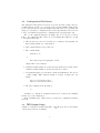
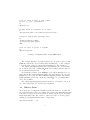
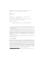
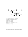
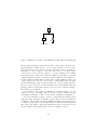
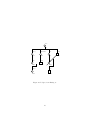
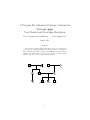
A Program For Automatic Pedigree Construction
With pst-pdgr
User Manual and Algorithm Description
Boris Veytsman, [email protected]
Leila Akhmadeeva
March 2012
Abstract
The set of macros in pst-pdgr package allows to typeset complex pedigrees. However, a manual placement of pedigree symbols on a canvas is a
time-consuming task. This program produces TEX files from spreadsheets
with the data on inheritance for a large class of pedigrees. It has a simple
interface and can be used for quite complex pedigrees.
I:1
I:2
I:3
I:4
b
II:1
III:1
II:2
II:3
III:2
1
III:3
III:4
Contents
I
User Manual
4
1 Introduction
4
2 Installation
2.1 System Requirements . . . . . . . . . . . . . . . . . . . . . . . .
2.2 Unix/Linux Installation . . . . . . . . . . . . . . . . . . . . . . .
2.3 Installation in Other Systems . . . . . . . . . . . . . . . . . . . .
4
4
4
5
3 Configuration
3.1 Configuration Variables and
3.2 Configuration File Format .
3.3 TEX Output Setup . . . . .
3.4 What to Print . . . . . . . .
3.5 Language and Encoding . .
3.6 Fonts . . . . . . . . . . . . .
3.7 Lengths . . . . . . . . . . .
3.8 Scaling and Rotation . . . .
Location of Configuration
. . . . . . . . . . . . . . .
. . . . . . . . . . . . . . .
. . . . . . . . . . . . . . .
. . . . . . . . . . . . . . .
. . . . . . . . . . . . . . .
. . . . . . . . . . . . . . .
. . . . . . . . . . . . . . .
4 Running the Program
4.1 Program Invocation And Options . . . .
4.2 Data File . . . . . . . . . . . . . . . . .
4.3 Twins . . . . . . . . . . . . . . . . . . .
4.4 Abortions . . . . . . . . . . . . . . . . .
4.5 Childlessness and Infertility . . . . . . .
4.6 Ordering Siblings and Marriage Partners
4.7 Consanguinic Unions . . . . . . . . . . .
4.8 Language-Dependent Keywords . . . . .
II
.
.
.
.
.
.
.
.
.
.
.
.
.
.
.
.
.
.
.
.
.
.
.
.
.
.
.
.
.
.
.
.
.
.
.
.
.
.
.
.
.
.
.
.
.
.
.
.
.
.
.
.
.
.
.
.
.
.
.
.
.
.
.
.
File
. . .
. . .
. . .
. . .
. . .
. . .
. . .
.
.
.
.
.
.
.
.
.
.
.
.
.
.
.
.
.
.
.
.
.
.
.
.
5
5
6
6
7
8
8
9
9
.
.
.
.
.
.
.
.
.
.
.
.
.
.
.
.
.
.
.
.
.
.
.
.
.
.
.
.
.
.
.
.
10
10
11
13
13
13
19
26
26
Algorithm Description
.
.
.
.
.
.
.
.
.
.
.
.
.
.
.
.
29
5 Introduction
29
6 Main Algorithm
29
7 Algorithm for Sorting Siblings and Marriage Partners
30
8 Modifications for Consangunic Unions
31
9 Conclusion
31
10 Acknowledgements
32
2
List of Figures
1
2
3
4
5
6
7
8
9
10
11
Example of the Typeset Pedigree in English (Data File from Listing 7) . . . . . . . . . . . . . . . . . . . . . . . . . . . . . . . . .
Example of the Typeset Pedigree in Russian (Data File from
Listing 7) . . . . . . . . . . . . . . . . . . . . . . . . . . . . . . .
Example of a Pedigree with Twins (Data File from Listing 8) . .
Example of a Pedigree with Abortions (Data File from Listing 9)
Example of a Pedigree with Childlessness (Data File from Listing 10) . . . . . . . . . . . . . . . . . . . . . . . . . . . . . . . . .
Pedigree from Listing 12 . . . . . . . . . . . . . . . . . . . . . . .
Pedigree from Listing 12 . . . . . . . . . . . . . . . . . . . . . . .
Pedigree from Listing 13 . . . . . . . . . . . . . . . . . . . . . . .
Pedigree from Listing 14 . . . . . . . . . . . . . . . . . . . . . . .
Pedigree from Listing 15 . . . . . . . . . . . . . . . . . . . . . . .
Subpedigrees and Downward Tree . . . . . . . . . . . . . . . . . .
15
16
17
18
20
22
23
24
25
27
30
List of Tables
1
Keywords in Different Languages . . . . . . . . . . . . . . . . . .
28
List of Listings
1
2
3
4
5
6
7
8
9
10
11
12
13
14
15
Configuration File: Setting TEX Output . . . . . . . .
Configuration File: Choosing Fields to Print . . . . . .
Configuration File: Choosing Language and Encoding
Configuration File: Choosing Fonts . . . . . . . . . . .
Configuration File: Choosing Lengths . . . . . . . . .
Configuration File: Choosing Scaling and Rotation . .
Examples of Data Files (English and Russian) . . . . .
Example of Data File with Twins . . . . . . . . . . . .
Example of Data File with Abortions . . . . . . . . . .
Example of Data File with Childlessness . . . . . . . .
A Data File with a Sorting Problem . . . . . . . . . .
First Solution to the Problem in Listing 11 . . . . . .
Second Solution to the Problem in Listing 11 . . . . .
A Pedigree with Unavoidable Self-Intersections . . . .
A Pedigree with Consanguinic Unions . . . . . . . . .
3
.
.
.
.
.
.
.
.
.
.
.
.
.
.
.
.
.
.
.
.
.
.
.
.
.
.
.
.
.
.
.
.
.
.
.
.
.
.
.
.
.
.
.
.
.
.
.
.
.
.
.
.
.
.
.
.
.
.
.
.
.
.
.
.
.
.
.
.
.
.
.
.
.
.
.
.
.
.
.
.
.
.
.
.
.
.
.
.
.
.
7
8
9
9
10
11
14
17
18
19
21
21
23
24
26
Part I
User Manual
1
Introduction
Medical pedigree is a very important tool for clinicians, genetic researchers and
educators. As stated in [1], “The construction of an accurate family pedigree is
a fundamental component of a clinical genetic evaluation and of human genetic
research.” The package pst-pdgr [2] provides a set of PSTricks macros (see [3])
to typeset pedigrees. In the framework of pst-pdgr the user manually chooses
coordinates for each pedigree node on the diagram. While this is relatively easy
for small pedigrees, this task becomes increasingly time-consuming for larger
ones. There may be several approaches to automate it. For example, one may
have data about the patients and their families in a spreadsheet or database.
Then it would be useful to generate pedigrees from such data. This is the aim
of the program pedigree described in this manual.
Spreadsheets and databases can export the data as separated values files
(“csv” files for Comma Separated Values). Our program reads these files and
outputs LaTeX code with pst-pdgr macros. We tried to make this code readable, so a user might tweak it if necessary.
Of course, manually produced LATEX code is more versatile than the automatically generated one. There are certain limitations for the program: 1. only
persons having common genes with the proband or the “starting person” are
included in the pedigree; 2. no adopted children, sperm donors or surrogate
mothers are shown on the pedigree; 3. only one disease is shown on the chart;
4. the support for consanguinic unions and inbreeding is rather experimental
(see Section 4.7). Subsequent versions of the program may ease some of these
limitations.
2
2.1
Installation
System Requirements
The program requires Perl version 5 or newer (it was tested with Perl v5.8.8, but
should work with any Perl-5). The LATEX macros require pst-pdgr version 0.3
(July 2007) or newer.
2.2
Unix/Linux Installation
If your system has a working make program, which is the usual case for Unixlike environments, the supplied Makefile installs the executable pedigree in
/usr/local/bin, the libraries in /usr/local/lib/site_perl and the manual
pages in /usr/local/man. This is done by the usual command make install.
4
Optionally you can install files in the doc and examples subdirectories in the
proper places in your system.
2.3
Installation in Other Systems
If your system does not have make, you need to manually perform the following:
1. Install the executable pedigree.pl to the place your system can find it.
2. Install the libraries: Pedigree.pm, directory Pedigree and all files in it
to the Perl search path. The latter is listed in the array @INC, which can
be checked by the command perl -V or its equivalent.
3
Configuration
3.1
Configuration Variables and Location of Configuration File
The program defaults are sufficient for most cases. However, if you want to
draw pedigrees in a language other than English, or to tweak the layout of the
pedigrees, you need to change the program configuration.
The behavior of the program pedigree is determined by configuration variables. There are several sources of configuration variables. They are (in the
order of increasing priority):
1. Program defaults.
2. The system configuration file1 /etc/pedigree.cfg. On TEXLive the system coniguration files are $TEXMFHOME/texmf-config/pedigree/pedigree.
cfg and $TEXMFLOCAL/pedigree/pedigree.cfg.
3. User configuration file2 $HOME/.pedigreerc.
4. The file specified by the -c option (see Section 4.1).
If a file mentioned in this list does not exists, the program silently3 continues.
Note that even if a configuration file with higher priority exists, the program
reads the files with lower priority first. The former overrides the latter, but
not precludes it from reading. In other words, if /etc/pedigree.cfg defines
variables $foo and $bar, and $HOME/.pedigreerc defines $bar and $baz, the
program takes $foo from the first file, and $bar and $baz from the second one.
1 On
Unix-like systems, where /etc exists
Unix-like systems, where $HOME exists
3 Unless -d option is selected, see Section 4.1
2 On
5
3.2
Configuration File Format
All configuration files mentioned in Section 3.1, have the same format. They are
actually snippets of Perl code, executed by the program pedigree. This means,
by the way, that all precautions usually taken with respect to programs and
scripts, are relevant for configuration files as well. In particular, it is a bad idea
to have world-writable system-wide configuration file /etc/pedigree.cfg.
The code in configuration files is very simple, and one does not need to know
Perl to edit configuration files. There are several simple rules which are enough
to understand these files:
1. All text after # to the end of the line is a comments. In particular, the
lines starting with #, are comment lines.
2. Perl commands must end by semicolon ;.
3. The commands like
$xdist =1.5;
or
@fieldsforprint = qw ( Name DoB );
assign values to the variables.
4. Variables starting with $ are scalars and take numerical or string values.
Variables starting with @ are arrays and take list of values.
5. A backslash in single quotes stands for itself, A backslash in double quotes
or inside <<END. . . END construction must be doubled. Compare the commands
$foo = ’\ documentclass ’;
$bar = " \\ documentclass " ;
6. The last command in the file must be
1;
A number of commented configuration files can be found in the examples
subdirectory of the distribution.
In the remaining parts of this section we describe the configuration variables
in detail.
3.3
TEX Output Setup
A number of variables determine what kind of TEX file is produced. An example
of their usage is shown on Listing 1.
6
# Do we want to have a full LaTeX
# file or just a fragment ?
#
$fulldoc =1;
# What kind of document do we want
#
$documentheader = ’\ documentclass { article } ’;
# Define additional packages here
#
$addtopreamble = < < END ;
\\ usepackage { pst - pdgr }
END
# Do we want to print a legend ?
#
$printlegend =1;
Listing 1: Configuration File: Setting TEX Output
The variable $fulldoc determines whether the program produces a full
LATEX file with header and preamble (when $fulldoc=1), or just a snippet
to be included in a larger document (when $fulldoc=0). The default is 1.
The variable $documentheader is used when $fulldoc is 1. It determines
the document class of the resulting LATEX file. The default is article class, set
by \documentclass{article}.
By default the preamble of the LATEX file created when $fulldoc is 1, contains only the line \usepackage{pst-pdgr} and, if the language chosen is not
English (see Section 3.5), the calls of babel and inputenc packages. The variable
$addtopreamble, if set, may contain any other LATEX code you might wish to
add to the preamble.
The variable $printlegend determines whether to add legend to the pedigree. The default value is 1, and the legend is printed.
3.4
What to Print
The next groups of configuration variables sets the information to be printed in
the legend and on the pedigree. It consists of two arrays: array @fieldsforlegend
is the list of fields (see Section 4.2) which are included in the legend, and array
@fieldsforchart is the list of fields to print near each node in the pedigree
(Listing 2). Setting @fieldsforchart to empty array:
@fieldsforchart = ();
7
# Fields to include in the legend .
# Delete Name for privacy protection .
#
@fieldsforlegend = qw ( Name DoB DoD Comment );
#
# Fields to put at the node .
# Delete Name for privacy protection .
#
@fieldsforchart = qw ( Name );
Listing 2: Configuration File: Choosing Fields to Print
prevents putting additional information on the pedigrees.
The field names are described in Section 4.2. Note that AgeAtDeath is
a special field: it is the age at death (or empty) calculated as the difference
between the death date and the birth date.
3.5
Language and Encoding
The next group of variables describes the language and encoding of the data
file input and the LATEX output. They are shown in Listing 3. The variable
$language at present can have one of two values: english (the default) or
russian. If the value is russian, the output document preamble includes the
line
\ usepackage [ russian ]{ babel }
The variable $encoding sets the encoding of the LATEX file if the language is not
English. By default it is cp1251, if the language is Russian. Set it to koi8-r
to choose KOI8 encoding. It is worth to note that the data file and the output
LATEX file are assumed to have the same language and encoding.
If $language is not english, the program recognizes both English and native
names of the fields in the data file (see Section 4.2).
3.6
Fonts
There are two kinds of text on the chart: the text above a node and the text
below a node4 . The fonts for them are set by the variables $belowtextfont (by
default \small) and $abovetextfont (by default \scriptsize). Any LATEX
font declaration like \sffamily or \itshape is allowed here. See Listing 4 for
an example of usage.
4 The T X package [2] also allows to place text at both sides of the node, but the program
E
pedigree currently does not use this feature.
8
#
# Language
#
# $language =" russian ";
$language = " english " ;
#
# Override the encoding
#
# $encoding =" koi8 - r ";
Listing 3: Configuration File: Choosing Language and Encoding
#
# Fonts for the chart
#
$belowtextfont = ’\ small ’;
$abovetextfont = ’\ scriptsize ’;
Listing 4: Configuration File: Choosing Fonts
3.7
Lengths
The next group of variables (Listing 5) sets the distances between the key elements of the chart. All lengths are in centimeters (actually, in units, are defined
in PSTricks [3]).
The variable $descarmA sets the length of the first segment of the descent
line: from the parent node to the sibs line, as measured from the center of the
parent (see [2] for more details). By default it is 0.8.
The variables $xdist and $ydist set the distances between the nodes along
horizontal and vertical axes correspondingly. The default for both is 2.
3.8
Scaling and Rotation
Complex pedigrees might be too large to fit on a page. In this case a scaling
and (or) rotation might be necessary to print the chart. Of course, changing
the lengths described in Section 3.7 might also help, but the scaling described
here also changed the size of the pedigree symbols.
There are three variables controlling the scaling and rotation of pedigrees:
$maxW, $maxH and $rotate (see Listing 6). The variables $maxW and $maxH are
the maximal width and height of the chart in centimeters. Setting any of them
to zero disables scaling.
9
#
# descarmA in cm
#
$descarmA = 0.8;
#
# Distances between nodes ( in cm )
#
$xdist =2;
$ydist =2;
Listing 5: Configuration File: Choosing Lengths
The scaling works as follows. If both height and width of the pedigree are
smaller than the limits, no scaling is done. In the other case the chart is scaled
while preserving the aspect ratio (by changing the value of unit, see [3]) to fit
into the limits.
The variable $rotate sets the orientation of the chart. If it is no, the
pedigree is never rotated, while if it yes, it is always rotated ninety degrees
counterclockwise. If this variable is set to maybe (the default), the program
compares the scaling for the non-rotated and rotated pedigrees, and chooses the
orientation for which the scaling is closer to one.
4
4.1
Running the Program
Program Invocation And Options
The program pedigree is a command line program. It reads the data from
a text file input_file and produces an output file with LATEX macros. The
format of the input file is described in Section 4.2. The program invocation is:
pedigree [-c configuration_file] [-d] [-o output_file]
[-s start] input_file
(the square brackets show optional arguments).
All arguments but input_file are optional. They are described below.
The option -c selects a configuration file. The format of the configuration
file is described in Section 3.1. If this option is absent, the program uses its own
default parameters, or system-wide or user’s defaults, as explained in Section 3.1.
The option -d selects debugging mode. In this mode a lot of debugging
messages are dumped to stderr.
The parameter -o provides the name of the output file. Both input_file
and output_file can be “-”, which means stdin for the input and stdout for
the output. If the parameter -o is absent, the program tries to guess the name
10
#
# Maximal width and height of the pedigree in cm .
# Set this to 0 to switch off scaling
#
$maxW = 15;
$maxH = 19;
#
# Whether to rotate the page . The values are
# ’ yes ’, ’ no ’ and ’ maybe ’
# If ’ maybe ’ is chosen , the pedigree is rotated
# if this provides better scaling
#
$rotate = ’ maybe ’;
Listing 6: Configuration File: Choosing Scaling and Rotation
of the output file from the name of the input file. If the input file is foo.csv,
the output file will be foo.tex. On the other hand, if the input file is stdin,
the output file is stdout.
Usually pedigrees are built starting from the proband5 . Only the people
that share genes with the proband, are shown on the pedigree. However, in
some cases, for example when there is no proband, or where there are several
probands, it is neccessary to override this default and tell the program from
which person to start. This is done using the option -s. If it is present, it
must be followed by the Id of a person in the data file (see Section 4.2 for the
discussion of Id).
The option -v is special. The invocation pedigree -v outputs the version
and license information.
4.2
Data File
The input for the program is a separated values file. Usually such files are called
CSV for “comma separated values”. However, this program uses the vertical
bar (“pipe”) | as a separator. Each line of this file is a record. The lines are
separated by pipes into fields. Most SQL programs produce such files by default.
Spreadsheet programs will make them if you choose “Save As. . . ” option, and
select | as the field separator, and empty text delimiter. We sometimes will
call the records “rows” and the fields “columns” to use the familiar spreadsheet
metaphor. Normally each row corresponds to a person in a pedigree. We will
call this person the current person when describing the fields.
5 The proband is the first person among the relatives who came to a geneticist; he or she
is the primary patient.
11
The width of the fields may not be the same in all rows (or, in other words,
the pipes | may be disaligned). We make them aligned in the examples included
in this manual just to make the text more readable.
The first line of the data file contains the names of the fields (“column
headers”). The fields in the subsequent lines must match the order of the
headers. An empty field must be still included (as || or | |). Otherwise the
order of columns is arbitrary as long as it is the same for all rows (i.e. matches
the order of “column headers” in the first line).
All fields but Id are optional. If the value is empty for all rows, the corresponding column can be dropped. If applicable, the default values for this field
will be substituted by the program.
On the other hand the data file can include any additional columns as long
as their names do not clash with the names listed below and the special name
AgeAtDeath. These additional columns can be included in the chart or legend
as described in Section 3.4.
Here is the list of columns and explanation of their meaning:
Id: Each line (including the special lines described below) must have a unique
Id. The Id may contain only Latin letters and numbers, and start with a
letter.
Name: The name of the person described in the current row. There are also
special names when the current row describes abortions or infertility. They
are described below. The names should not contain “special symbols” like
#, $, %, , ˆ, etc.
Sex: The gender of a person. This column may have one of two values: male or
female. The empty value corresponds to a person with unknown gender.
DoB: The date of birth for the current person. The format is YYYY.MM.DD. If
the date of birth is not known, the field may be empty or the keyword
unknown may be used.
DoD: The date of death for current person. The format is the same as for
DoB: YYYY.MM.DD. If this field is empty, the corresponding person is alive.
For deceased persons with an unknown date of death use the keyword
unknown. Note the subtle difference between the fields DoB and DoD: an
empty value for DoB is means “unknown birth date” while for DoD it means
that there is no date of death at all.
Mother: The Id of the mother of the person (or empty).
Father: The Id of the father of the person (or empty).
Proband This field can be either yes for the probands, or empty (or no) for
other persons. Note that if a pedigree has no probands or several probands,
the program does not know, from which node to start the pedigree. Therefore in this case the option -s must be used to explicitly set the Id of the
starting chart node (see Section 4.1).
12
Condition: This column can have the values normal, obligatory, asymptomatic
or affected. If it is empty, the default value normal is assumed.
Comment: A comment about the person.
Twins: If the current person has twins, they are listed in this column separated
by spaces and (or) commas. See Section 4.3 for more details.
Type: This column is used in certain special cases. For abortions it shows the
type of the abortion (Section 4.4), for childless people and marriages it
shows the type of childnessness (Section 4.5), and for twins it shows the
type of twins (Section 4.3).
SortOrder: This column is used when the algorithm for sorting siblings and
unions gives a wrong result, and a manual correction is needed. See Section 4.6 for the explanation and examples.
Examples of data files (in English and Russian) are shown in Listing 7 (the
Russian keywords are discussed in Section 4.8).
4.3
Twins
The column Twins (see Section 4.3) lists all Ids of all twins of the given person.
The column Type can be used to show the type of the twins. The empty value
means polyzygotic twins, monozygotic means monozygotic twins, and qzygotic
is used in the case when the type of twins is under doubt. An example of a data
file with twins is shown on Listing 8, and the corresponding pedigree on Figure 3.
4.4
Abortions
Aborted pregnancies are described by a special entry in the data file. The field
Name has the value #abortion; the symbol # is used to show that this is a
special value. The columns Sex, DoB, Mother, Father and Condition have the
usual meaning. The special column Type is either empty or be equal to sab for
self-abortions.
4.5
Childlessness and Infertility
Childlessness is can be a property of a person or a union between two persons.
Therefore in this implementation we use a special row rather than a column to
report it. As other rows, this one has a unique Id. The Name column should
have a special entry #childless. Like #abortion (Section 4.4), this special
name starts with # to distinguish it from “real” names. There are four other
columns that have meaning for this row:
Mother: The Id of the childless female.
13
Listing 7: Examples of Data Files (English and Russian)
14
|Sex
|DoB
| DoD
|Mother|Father|Proband|Condition |Comment
|male |1970/02/05|
|M1
|F1
| yes
| affected|Evaluated 2005/12/01
|female|1940/02/05|
|GM2
|GF2
|
| normal |
|male |1938/04/03|
|GM1
| GF1 |
|affected |
|female|1902/07/01|1975/12/13|
|
|
|asymptomatic
|male |unknown
|unknown
|
|
|
| normal
|male |1905/11/01|
|
|
|
| normal |
|female|1910/03/03|
|
|
|
| normal |
|female|1972/12/25|
|M1
|F1
|
| affected
|male |1975/11/12|
|M1
|F1
|
| normal
|female|1941/09/02|
|GM1
| GF1 |
| obligatory|Aunt of the proband
|female|1969/12/03|
|A1
|
|
| affected | Cousin of the proband
Идент|ФИО
|Пол|Рожд
|Умер
|Мать|Отец|Пробанд|Состояние | Комментарий
P
|Иванов Сергей Петрович |муж|1965/08/06|
|M1 |F1 |да
|больн
|
M1
|Иванова Любовь Ивановна|жен|1935/12/01|2005/10/01|
|
|
|норм
F1
|Иванов Петр Ильич
|муж|неизв
|2003/01/25|
|
|
|облигат
S1
|Иванова Анна Петровна |жен|1968/05/05|
|M1 |F1 |
|норм
K1
|Иванов Иван Сергеевич |муж|1990/12/01|
|
|P
|
|асимп |Генетич. иссл. 2005/12/08
K2
|Иванова Дарья Сергеевна|жен|1995/03/24|
|
|P
|
|норм
|Генетич. иссл. 2005/12/08
Id |Name
P |John Smith
M1 |Mary Smith
F1 |Bill Smith
GM1|Joan Smith
GF1|Joseph Smith
GF2|Jim Brown
GM2|Lisa Brown
S1 |Rebecca Smith
S2 |Alexander Smith
A1 |Ann Gold
C1 | Jenny Smith
Joseph Smith
Joan Smith
Jim Brown
Lisa Brown
I:1
I:2
I:3
I:4
Ann Gold
Bill Smith
Mary Smith
II:1
II:2
II:3
b
Jenny Smith
John Smith
Rebecca Smith Alexander Smith
III:1
III:2
III:3
III:4
I:1 Joseph Smith; born: unknown; age at death: unknown.
I:2 Joan Smith; born: 1902/07/01; age at death: 73.
I:3 Jim Brown; born: 1905/11/01.
I:4 Lisa Brown; born: 1910/03/03.
II:1 Ann Gold; born: 1941/09/02; Aunt of the proband.
II:2 Bill Smith; born: 1938/04/03.
II:3 Mary Smith; born: 1940/02/05.
III:1 Jenny Smith; born: 1969/12/03; Cousin of the proband.
III:2 John Smith; born: 1970/02/05; Evaluated 2005/12/01.
III:3 Rebecca Smith; born: 1972/12/25.
III:4 Alexander Smith; born: 1975/11/12.
Figure 1: Example of the Typeset Pedigree in English (Data File from Listing 7)
15
Иванов Петр Ильич
Иванова Любовь Ивановна
I:1
I:2
b
Иванов Сергей Петрович Иванова Анна Петровна
II:1
II:2
Иванов Иван Сергеевич Иванова Дарья Сергеевна
III:1
III:2
I:1 Иванов Петр Ильич; род. неизв.; ум. в возр. неизв..
I:2 Иванова Любовь Ивановна; род. 1935/12/01; ум. в возр. 70.
II:1 Иванов Сергей Петрович; род. 1965/08/06.
II:2 Иванова Анна Петровна; род. 1968/05/05.
III:1 Иванов Иван Сергеевич; род. 1990/12/01; Генетич. иссл. 2005/12/08.
III:2 Иванова Дарья Сергеевна; род. 1995/03/24; Генетич. иссл. 2005/12/08.
Figure 2: Example of the Typeset Pedigree in Russian (Data File from Listing 7)
16
Id
F0
A0
A1
A2
B1
B2
B3
C1
C2
C3
C4
|Name |Sex
|DoB
|DoD
|Mother|Father|Proband|Twins|Type
|Adam |male |unknown
|unknown
|
|
|
|
|
|Sam
|male |1950.01.03|unknown
|
|F0
|
| A1 |qzygotic
|John |male |1950.01.03|2005.04.12|
|F0
|
| A0 |qzygotic
|Jane |female|1951.14.15|
|
|
|
|
|
|Jack |male |1975.05.06|
|A2
|A1
|
|B2
|monozygotic
|Mike |male |1975.05.06|
|A2
|A1
|
|B1
|monozygotic
|Pam
|female|1973.11.01|
|A2
|A1
|
|
|
|Jane |female|1998.12.04|
|
|B1
|
|C2,C3|
|John |male |1998.12.04|
|
|B1
|
|C1,C3|
|George|male |1998.12.04|
|
|B1
| yes |C1,C2|
|Ann
|female|2003.02.04|
|
|B1
|
|
|
Listing 8: Example of Data File with Twins
Adam
I:1
Sam
?
II:1
John
Jane
II:2
II:3
Pam
Jack
Mike
III:1
III:2
III:3
George
John
Jane
Ann
IV:1
IV:2
IV:3
IV:4
Figure 3: Example of a Pedigree with Twins (Data File from Listing 8)
17
Id
A0
B1
B2
B3
|Name
|Sex
|DoB
|DoD
|Ann
|female|1970.06.15|
|#abortion|female|1990.03.01|
|#abortion|male |2000.10.10|
|John
|male |2002.12.01|
|Mother|Proband|Condition|Type
|
|
|affected |
|A0
|
|affected |
|A0
|
|
|sab
|A0
|yes
|affected |
Listing 9: Example of Data File with Abortions
Ann
I:1
female
male
II:1
II:2
John
II:3
I:1 Ann; born: 1970.06.15.
II:1 abortion; born: 1990.03.01.
II:2 abortion; born: 2000.10.10.
II:3 John; born: 2002.12.01.
Figure 4: Example of a Pedigree with Abortions (Data File from Listing 9)
18
Id |Name
A0 |John
B1 |James
B1c|#childless
B2 |Ann
B2c|#childless
|Sex
|Mother|Father|Proband|Type
|male |
|
|
|
|male |
|A0
|
|
|male |
|B1
|
|infertile
|female|
|A0
|yes
|
|
|B2
|
|
|
|Comment
|
|
|anospermia
|
|
Listing 10: Example of Data File with Childlessness
Father: The Id of the childless male. If both Mother and Father columns are
not empty, the entry describes the union between the Father and Mother.
Of only Mother or Father is not empty, the entry describes the state of
the corresponding person.
Type: This column might be either empty or have a keyword infertile. In
the latter case the childlessness of the person or union is caused by a
proven infertility.
Comment: The vaule of this column is shown under the childlessness symbol
on the chart. Put there a short description of the cause of childlessness,
like anospermia or vasectomy.
An example of a pedigree with childlessness is shown on Listing 10 and Figure 5.
4.6
Ordering Siblings and Marriage Partners
The generations in pedigrees are ordered in vertical direction, from up do down.
How should we order the people on the same generation, i.e. siblings and marriage partners?
Usually two rules are used:
1. The siblings are ordered from the oldest on the left to the youngest to the
right.
2. In marriage or other union the male is to the left, and the female is to the
right.
However, the combination of these rules might lead to the situation when marriage lines intersect the parental lines. Therefore the rule 1 is usually implicitly
modified:
1a. The are ordered from the oldest on the left to the youngest to the right.
However, if a sibling’s marriage is shown on a pedigree, this sibling is
always the rightmost (male) or the leftmost (female).
19
John
I:1
James
Ann
II:1
II:2
anospermia
Figure 5: Example of a Pedigree with Childlessness (Data File from Listing 10)
The program follows these rules. It is enough to draw pedigrees in most cases.
In particular, they always produce correct pedigrees if there is only one marriage shown. However, in complex cases these rules fail, as shown on Listing 11
and Figure 6. It is possible to extend the rules above to account for these
cases, however we chose another solution: to provide a facility for the manual
intervention in the sorting and ordering algorithm. For this purpose a special
column SortOrder is used. It can have positive numbers greater than 1 or
negative numbers smaller than -1. If the value of this column is positive, the
corresponding person is moved to the left when sorting siblings and to the right
when sorting marriage partners. If it is negative, the opposite sorting rule is applied (see Section 7 for more detailed discussion). Note that sibling sorting and
marriage partners sorting must work in opposite directions, otherwise marriage
lines intersect paternal lines.
Let us return to the pedigree on Listing 11. To improve Figure 6 we can
either move Peter to the right or Lucy to the left. The first solution is shown
on Listing 12 and Figure 7. The second is shown on Listing 13 and Figure 8.
Of course sometimes a pedigree cannot be drawn without self-intersections
with any sorting of siblings. An example of such pedigree is shown on Listing 14
and Figure 9. Obviously no amount of shuffling the siblngs can help in his case.
If the program cannot avoid self-intersection of marriage lines and parental
lines despite automatics sorting and manual intervention, as the last resort it
creates a multi-segment marriage line, as shown on Figures 6 and 9.
20
Id
A0
B1
B2
B3
B4
C1
C2
C3
C4
D1
D2
|Name
|John
|Joan
|Jane
|Bill
|Peter
|Jack
|Sam
|Ann
|Lucy
|Mark
|Dina
|Sex
|DoB
|Father|Mother|Proband
|male |1915.06.15|
|
|
|female|1940.03.02|A0
|
|
|female|1942.07.07|A0
|
|
|male |1944.12.01|A0
|
|
|male |1941.05.01|
|
|
|male |1963.12.01|B4
|B2
|
|male |1961.08.26|
|B1
|
|female|1965.11.12|
|B3
|
|female|1965.12.11|
|
|
|male |1989.06.21|C1
|C4
|yes
|female|1991.12.02|C1
|C4
|
Listing 11: A Data File with a Sorting Problem
Id
A0
B1
B2
B3
B4
C1
C2
C3
C4
D1
D2
|Name
|John
|Joan
|Jane
|Bill
|Peter
|Jack
|Sam
|Ann
|Lucy
|Mark
|Dina
|Sex
|DoB
|Father|Mother|Proband|SortOrder
|male |1915.06.15|
|
|
|
|female|1940.03.02|A0
|
|
|
|female|1942.07.07|A0
|
|
|
|male |1944.12.01|A0
|
|
|
|male |1941.05.01|
|
|
| 3
|male |1963.12.01|B4
|B2
|
|
|male |1961.08.26|
|B1
|
|
|female|1965.11.12|
|B3
|
|
|female|1965.12.11|
|
|
|
|male |1989.06.21|C1
|C4
|yes
|
|female|1991.12.02|C1
|C4
|
|
Listing 12: First Solution to the Problem in Listing 11
21
Figure 6: Pedigree from Listing 12
22
III:2
III:1
II:3
Sam
II:2
II:1
Joan
Jack
Jane
Peter
I:1
John
III:3
Ann
II:4
Bill
Dina
IV:2
Mark
IV:1
III:4
Lucy
John
I:1
Joan
Bill
Jane
Peter
II:1
II:2
II:3
II:4
Sam
Ann
Jack
Lucy
III:1
III:2
III:3
III:4
Mark
Dina
IV:1
IV:2
Figure 7: Pedigree from Listing 12
Id
A0
B1
B2
B3
B4
C1
C2
C3
C4
D1
D2
|Name
|John
|Joan
|Jane
|Bill
|Peter
|Jack
|Sam
|Ann
|Lucy
|Mark
|Dina
|Sex
|DoB
|Father|Mother|Proband|SortOrder
|male |1915.06.15|
|
|
|
|female|1940.03.02|A0
|
|
|
|female|1942.07.07|A0
|
|
|
|male |1944.12.01|A0
|
|
|
|male |1941.05.01|
|
|
|
|male |1963.12.01|B4
|B2
|
|
|male |1961.08.26|
|B1
|
|
|female|1965.11.12|
|B3
|
|
|female|1965.12.11|
|
|
| -3
|male |1989.06.21|C1
|C4
|yes
|
|female|1991.12.02|C1
|C4
|
|
Listing 13: Second Solution to the Problem in Listing 11
23
John
I:1
Peter
Jane
Joan
Bill
II:1
II:2
II:3
II:4
Lucy
Jack
Sam
Ann
III:1
III:2
III:3
III:4
Mark
Dina
IV:1
IV:2
Figure 8: Pedigree from Listing 13
Id
A0
B1
B2
C1
F1
G1
G2
H1
K1
M1
P1
R1
X1
|Name
|John
|Sam
|Ann
|Paul
|Scott
|Simon
|Sarah
|Lola
|Jim
|Jane
|Simon
|Pam
|James
|Sex
|DoB
|Father|Mother|Proband
|male |1915.06.15|
|
|
|male |1935.12.04|A0
|
|
|female|1937.03.02|A0
|
|
|male |1952.10.03|B1
|
|
|male |1912.02.01|
|
|
|male |1934.09.17|F1
|
|
|female|1936.12.19|F1
|
|
|female|1960.04.13|G2
|
|
|male |1962.11.05|G1
|B2
|
|female|1917.02.13|
|
|
|male |1935.10.04|
| M1
|
|female|1964.02.05|P1
|
|
|male |1988.07.12|K1
|R1
|yes
Listing 14: A Pedigree with Unavoidable Self-Intersections
24
Figure 9: Pedigree from Listing 14
25
Jim
III:2
III:1
II:2
II:1
Lola
Simon
II:3
Ann
I:2
I:1
Sarah
John
Scott
III:3
Paul
II:4
Sam
IV:1
James
III:4
Pam
II:5
Simon
I:3
Jane
Id
A0
B1
B2
B3
B4
C1
C2
C3
D1
D2
|Name
|Jane
|John
|Ann
|Samantha
|Nancy
|Mary
|Paul
|Jane
|Jack
|Laura
|Sex
|Father|Mother|Proband|DoB
|female|
|
|
|1908.12.12
|male |
|A0
|
|1936.12.15
|female|
|A0
|
|1934.04.17
|female|
|A0
|
|1932.12.03
|female|
|A0
|
|1928.01.05
|female|
|B2
| yes
|1955.08.26
|male |
|B3
|
|1964.05.07
|female|
|B4
|
|1950.11.03
|male |B1
|C1
|
|1975.07.01
|female|C2
|C3
|
|1974.09.05
Listing 15: A Pedigree with Consanguinic Unions
4.7
Consanguinic Unions
Consanguinic unions present a technical problem for the program (see the discussion in Section 8). Therefore the support of consanguinicity is experimental
for this release.
There is a number of limitations for consanguinic unions in the data file at
present. First, the consanguinic unions should not in the direct lineage of the
proband or the person from which the pedigree starts. In many cases this limitation can eliminated by using -s option (see Section 4.1) to choose a different
starting point for the pedigree. Second, the children of consanguinic unions
might appear not centerd on the charts. An example of a pedigree with consanguinic marriages is shown on Listing 15, and the corresponding chart is shown
on Figure 10. The drawbacks of the program are evident from the positions of
Laura nad Jack on these charts.
4.8
Language-Dependent Keywords
At present the program pedigree can work with English and Russian languages.
As discussed in Section 3.5, the language options chooses both the languages
of input and output files. It is easy to add new languages to the scheme by
expanding the library Pedigree::Language.pm in the distribution.
The English language is the default. Moreover, if the Russian option is
chosen, English keywords are still recognized in the input file.
The English and Russian keywords are listed in Table 1. Note that some
keywords have variants; they are listed in the table as well.
26
Jane
I:1
Nancy
Samantha
Ann
John
II:1
II:2
II:3
II:4
Jane
Paul
Mary
III:1
III:2
III:3
Laura
Jack
IV:1
IV:2
Figure 10: Pedigree from Listing 15
27
English keyword
Field Names
Id
Name
Sex
DoB
DoD
Mother
Father
Proband
Condition
Comment
Type
Twins
SortOrder
Field Values
male
female
unknown
yes
no
normal
obligatory
asymptomatic
affected
infertile
sab
monozygotic
qzygotic
Special Names
#abortion
#childless
English variants
Russian keywords
Sort
Идент
ФИО
Пол
Рожд
Умер
Мать
Отец
Пробанд
Состояние
Комментарий
Тип
Близнецы
ПорядокСортировки, Сорт
муж, м
жен, ж
неизв, неизвестно
да
нет
норм, здоров
облигат
асимп
больн, болен
бесплодн
выкидыш
монозиготн, монозиг, однояйцев
?
obligat
asymp
affect
monzygot
qzygot, ?
#аборт
#бездетн
Table 1: Keywords in Different Languages
28
Part II
Algorithm Description
5
Introduction
This part is intended for advanced users and is not neccessary for runnuing the
program.
The problem of nicely typesetting graphs is one of the classical problems in
the Computer Science [4]. One of the earliest algorithms here is the classical
algorithm for layered rooted trees by Reingold and Tilford [4, § 3.1]. This
algorithm was implemented by PSTricks [3]. However, many pedigrees are not
trees [2]. If we consider a subset of pedigrees where inbreeding is absent, the
pedigrees become trees. However, even in this case the the tree is not necessary
layered, as can be seen from Figure 1. Therefore a new approach generalizing
Reingold-Tilford algorithm is necessary. This approach is based on the analysis
of the structure of pedigrees and is sketched in the remainder of this manual.
6
Main Algorithm
A pedigree consists of nodes (vertices), connected by lines (edges). If there is
no inbreeding, the graph is acyclic. There are two kinds of nodes in the graph:
person nodes (squares and circles on Figures 1 and 2) and marriage nodes,
which are nameless on the figures. We will use the notation “male spouse-female
spouse” for such nodes, so the marriage nodes on Figure 1 are I:1-I:2, I:3-I:4
and II:2-II:3. A node has a precedessor and children. A marriage node does not
have a precedessor, but has male spouse and female spouse (it is customary to
put male spouses to the left and female spouses to the right on pedigrees). Any
node has a downward tree of its children, grandchildren etc. The downward tree
may be empty.
Any node in an acyclic graph can be a root. However, in layered trees there
is a special root: the one that has no precedessor. Similarly we will call a local
root a node that has no predecessor. All marriage nodes are local roots. Some
person nodes can be local roots as well.
Let us first discuss the case where cobnsanguinic marriages are absent. In
this case a pedigree is a tree.
The proposed algorithm is recursive and starts from a local root. Strictly
speaking, it can start from any local root, but medical pedigrees have a special
person: proband, the person who was the first to be examined by genetic specialists (the proband is shown by an arrow drawn near the node on Figures 1
and 2). Therefore it makes sense to start from the local root which has proband
in its downward tree.
If this local root is a person node, the pedigree is the layered tree, and
Reingold-Tilford algorithm is sufficient. Therefore we should consider only the
29
Left subpedigree
I:1
Right subpedigree
I:2
I:3
I:4
Local root
b
b
II:1
II:2
III:1
II:3
III:2
III:3
Downward tree
III:4
Figure 11: Subpedigrees and Downward Tree
case when the local root is a marriage node. In this case we can typeset the
downward tree using Reingold-Tilford algorithm. The spouses do not belong to
this tree. However, each of them belongs to each own subpedigree. We will call
them left subpedigree and right subpedigree. We recursively apply our algorithm
to typeset left and right subpedigrees. Then we move the left subpedigree to
the right and right subpedigree to the left as far as we can without intersection
between them and the downward tree.
This process is shown on Figure 11. Obviously this algorithm converges and
leads to typesetting the pedigree without intersections between the subtrees and
subpedigrees.
7
Algorithm for Sorting Siblings and Marriage
Partners
When we create a marriage node, we want to put the male to the left and the
female to the right. When we then sort siblings, we want this male to be the
rightmost, and the female to be the leftmost. To do so, we assign to each node
the special quantity SortOrder. Initially all nodes have SortOrder equal to
zero, unless specifically set by the user in the input file (see Section 4.6). Then
we use the following rules:
1. When creating the the marriage node:
30
(a) If both spouses have equal SortOrder field, the male goes to the left,
the female goes to the right.
(b) Otherwise, the spouse with greater SortOrder goes to the left.
(c) If SortOrder of a spouse is 0, we set it to 1 (the spouse on the left)
or -1 (the spouse on the right).
2. When sorting siblings:
(a) The sibling with smaller SortOrder goes to the left.
(b) If both siblings have the same SortOrder, the oldest one goes to the
left.
8
Modifications for Consangunic Unions
Consanguinic unions present a problem for the described algorithm, because
pedigrees with them are no longer trees (see Figure 10).
In this release of the program we use the following hack. The direct lineage of
the proband (or, more generally, the starting node) may have both mothers and
fathers in the pedigree because they share genes from the starting node. If any
other person has both mother and father in the chart, his or her parents both
shared their genes with the starting node. Therefore they formed a consanguinic
union. In this case the children of this node appear in two subtrees: their
mother’s and their father’s.
We delete them from one of the subtrees (the one with lower generation
number), connect their parents with a double line (consanguinic union) and put
the descent line from the middle of the union to them.
There are two problems with this hack (see Section 4.7): the children of
consanguinic unions are not centered on the diagaram, and the hack fails if the
starting node itself is a descendant of a consanguinic union.
Probably the next releases will employ better algorithms for consanguinic
unions.
9
Conclusion
The algorithm seems to be efficient and producing nicely typeset pedigrees.
Since the input file format is simple, it may be used by the people without
special skills in LATEX. On the other hand, the TEX files produces are easy to
understand and edit manually if the need arises.
31
10
Acknowledgements
The authors are grateful to Herbert Voß for help with PSTricks code. The
support of TEX User Group is gratefully acknowledged. One of the authors
(LA) was supported by Russian Foundation for Fundamental Research (travel
grant 06-04-58811), Russian Federation President Council for Grants Supporting
Young Scientists and Flagship Science Schools (grant MD-4245.2006.7)
References
[1] Robin L. Bennett, Kathryn A. Steinhaus, Stefanie B. Uhrich, Corrine K.
O’Sullivan, Robert G. Resta, Debra Lochner-Doyle, Dorene S. Markei, Victoria Vincent, and Jan Hamanishi. Recommendations for standardized human pedigree nomenclature. Am. J. Hum. Genet., 56(3):745–752, 1995.
[2] Boris Veytsman and Leila Akhmadeeva.
Creating Medical
Pedigrees
with
PSTricks
and
LATEX,
July
2007.
http://ctan.tug.org/tex-archive/graphics/pstricks/contrib/pedigree/pst-pdgr.
[3] Timothy Van Zandt. PSTricks: PostScript Macros for Generic TEX, July
2007. http://ctan.tug.org/tex-archive/graphics/pstricks/base/doc.
[4] Giuseppe Di Battista, Peter Eades, Roberto Tamassia, and Ioannis G. Tollis.
Graph Drawing: Algortihms for the Visualization of Graphs. An Alan R. Apt
Book. Prentice Hall, New Jersey, 1999.
32