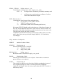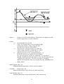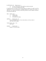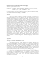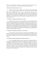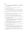
1
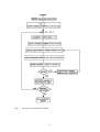
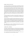
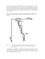
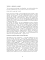
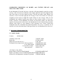
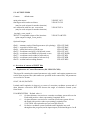
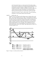
Second draft version 5th October 1995
Program VELEST USER’S GUIDE - Short Introduction
E. Kissling
Institute of Geophysics, ETH Zuerich
This short introduction corresponds to the VELEST Version 3.1 (10.4.95) by:
Edi KISSLING, Urs KRADOLFER, and Hansrudi MAURER
Institute of Geophysics and Swiss Seismological Service, ETH-Hoenggerberg
CH-8093 Zurich, Switzerland
Phone: +41 1 633 2605; Fax : +41 1 633 1065; Telex: 823480 eheb ch
E-Mail addresses:
[email protected]
(Internet)
[email protected]
[email protected]
1. Purpose and history of VELEST
Program VELEST is a FORTRAN77 routine that has been designed to derive 1-D
velocity models for earthquake location procedures and as initial reference models for
seismic tomography (Kissling 1988; Kissling et al. 1994). Originally written in 1976 by
W.L. Ellsworth and S. Roecker for seismic tomography studies (under program name
HYPO2D, see Ellsworth 1977; Roecker, 1978) VELEST has been modified by R.
Nowack (who also gave it its current name), C. Thurber, and R. Comer who
implemented (among other things) the layered-model raytracer (Thurber 1981). In
1984 E. Kissling and W. L. Ellsworth after modifications of the flow structure and
implementation of several new options used it to calculate a 'Minimum 1-D model'
(i.e., a well-suited 1-D velocity model for earthquake location and for 3-D seismic
tomography) for Long Valley area, California (Kissling et al., 1984). Since then
VELEST has been applied to local earthquake and controled-source data from several
areas in California, Alaska, Wyoming, Utah, and the Alps (Kissling 1988; Kradolfer
1989; Kissling and Lahr 1991; Maurer 1993). U. Kradolfer implemented the option to
use VELEST as single-event-location routine and H. Maurer reintroduced the option
to use both P- and S-wave data, separately or combined. Thanks to the cleaning efforts
of U. Kradolfer and of H. Maurer the code no longer suffers from quick-and-risky
programming by too many authors. The current version of VELEST has been tested to
correctly run under both UNIX (HP and SUN) and VMS (DEC) operating systems
with (optimized) standard FORTRAN77 compilers.
If you need a reference please use Kissling et al. (1994) (see reference list) or the
appropriate of the ones mentioned above. In order to avoid misunderstandings it is
recommended that you also mention the version of the program.
1
2. Simultaneous Inversion and Coupled Hypocenter-Velocity Model Problem
This USER«S GUIDE to VELEST is intended to provide a brief introduction on how
to run and use the program to simultaneously locate earthquakes and to calculate 1-D
(layered) velocity models with station corrections. As an introduction to the coupled
hypocenter-velocity model problem the reader is referred to Crosson (1976), Ellsworth
(1977), and Thurber (1981). The concept of a 'Minimum 1-D model' is described in
detail by Kissling (1988) and Kissling et al. (1995), who also provide several examples
of applications of such 1-D velocity models for both improved earthquake locations
and as initial reference models for 3-D seismic tomography. Kissling et al. (1994) -after
describing the effects of initial reference models on 3-D tomographic results- in an
appendix provide a brief overview over the procedure to be followed to calculate a
'Minimum 1-D model' with VELEST. The following USER’S GUIDE is written under
the assumption that the reader is vaguely familiar with the problems and solutions
described in the above mentioned publications (see reference list). Here only a brief
overview will be given.
Program VELEST (iteratively, i.e., "non-linearly") solves
* in 'simultaneous mode':
the coupled hypocenter-velocity model problem
for local earthquakes, quarry blasts, and shots; for
fixed velocity model and station corrections
VELEST in simultaneous mode performs the
Joint-Hypocenter-Determination (JHD).
* in 'single-event-mode':
the location problem for local earthquakes, blasts, and
shots.
The model consists of a (layered) 1-D velocity model and station corrections. In both
modes the forward problem is solved by ray tracing from source to receiver,
computing the direct, refracted, and (optionally) the reflected rays passing through the
1-D model. In both modes the inverse problem is solved by full inversion of the
damped least squares matrix [AtA+L] (A= Jacobi matrix, At=transposed Jacobi
matrix; L=damping matrix). Because the inverse problem is non-linear, the solution is
obtained iteratively, where one iteration consists of solving both the complete forward
problem and the complete inverse problem once (see Fig. 1). In 'single-event-mode' an
additional singular value decomposition of the symmetric matrix AtA (in this case a
4*4 matrix only) is performed in order to calculate the eigenvalues.
Due to the intrinsic ambiguity of the inverse problem the final solutions obtained by
VELEST are but a small part -and often the least significant part- of all the output of
this program. VELEST has been designed to allow great flexibility in the approach
and, therefore, a large number of options and control parameters must be set and
properly adjusted in the process. Though default values may be obtained from the
examples provided with the source code, the calculation of a Minimum 1-D model
requires multiple runs with VELEST to select and test control parameters appropriate
to the data set and to the problem. If you are in a hurry or if you are used to the idea
that proper computer programs always provide a unique solution that is either
2
obviously inappropriate or precise and correct, please accept the warning: To calculate
a Minimum 1-D model a single or even a few VELEST runs are useless, as they
normally do not provide any information on the model space (see chapt. 4)!
The principal procedure for simultaneous mode (and with minor modifications also for
single_event_mode) is summarized in the flowchart given in Fig. 1. The main (print)
output of VELEST reflects this procedure and provides detailed information about
many intermediate calculation steps even within one single iteration step. It is mainly
from these intermediate results that the appropriate control parameters are obtained
through many runs of VELEST.
Please do not use resolution calculation in simultaneous mode. There is a bug in this
part that will be fixed in version VELEST 3.2 by end of 1995.
3
Fig. 1
Overview of procedure VELEST
4
3. Installation of FORTRAN program VELEST:
VELEST version 3.1 may be obtained for UNIX (SUN and HP) machines and for
VAX/VMS (DEC) systems. Please check that you get the appropriate source code
among the files
-
VELESTUNIXSUN.F
VELESTUNIXHP.F
VELESTVMS.F .
In each case you also need the file VEL_COM.F that contains the common block
variables.The difference between the UNIX and VMS version are the I/O - file
attachments ("open" - calls) only. Thus, in the UNIX versions you will find aside of
each active line for opening call an additional line beginning with "cvms" with the open
calls in the VMS-system and vice versa in the VMS version are lines beginning with
"cunix" and the open calls for UNIX.The only system-dependent calls are found in the
two subroutines DATETIME and CPUTIMER; so if the program should be moved
onto another machine, only these two small subroutines located at end of the source
code have to be changed. Alternatively, delete all calls to these two routines which are
not essential for the main calculations (they just provide run-time information).
VELEST is currently set up to invert data in simultaneous mode from a maximum of
658 earthquakes (iepmax=658) and max. 50 shots or quary blasts (inshotsmax=50)
with max. 500 observations per event (maxobsperevent =500). Current setting also
allow a max. number of 500 stations in the station list (istmax=500), max. 2 velocity
models (itotmodels=2) with max. 100 layers per velocity model (inltot=100).
If you decide to need other dimensions please only adjust the parameters at the
beginning of the file VEL_COM.F and compile the source with an (optimized) F77
compiler.
In addition to the source you should also get a set of files providing examples of input
and output data for simultaneous mode. To each example there belong 5 types of files:
Input:
Output:
-
*.cmn
*.sta
*.mod
*.cnv
*.out
(control parameters)
(station list)
(initial velocity model)
(local earthquake data)
(main print output)
4. Calculation of Minimum 1-D model (simultaneous mode)
Solutions to the coupled hypocenter-velocity model problem consist of the
hypocenters, the velocity model, and station corrections. Each such solution may be
rated by comparing its corresponding (calculated) travel times with the measured
(observed) travel times. These travel time differences are called the misfit (or residuals)
of the solution and we may measure the total misfit by using any Norm. Most often the
5
RMS (root-mean-squared)-misfit of the solution is used.Consider any possible
combination of hypocenters, velocity model, and station corrections be rated by its
RMS misfit for a well-posed problem that would only have one solution with minimal
RMS. Such a situation could be represented by Figure 2a. In the case of the coupled
problem with local earthquake data, however, such a diagram displaying the RMS
misfit for various solutions most probably looks more like Figure 2b, where serveral
local RMS minima occur. In such situations the solution obtained by any iterative
algorithm strongly depends on the initial model and initial hypocenter locations.
Figure 2.
Quality estimate of solutions to the coupled problem. a: Simple case
with unique "best fit" solution. b: Normal case with several local
minima of RMS misfit.
Unfortunately, we do not a priori know this function (Fig. 2b) and, therefore, we must
search for different solutions with minimal misfit (RMS) by varying initial models and
hypocenter locations within reasonable but large bounds. Thus, the calculation of a
Minimum 1-D model amounts to a TRIAL-AND-ERROR process (for different initial
models) with internal non-linear (iterative) INVERSION procedure, performed by
VELEST.
Since VELEST does not automatically adjust layer thickness (as opposed to layer
velocities), the appropriate layering of the model must be found by a trial-and-error
process. Thus the calculation of a Minimum 1-D model normally starts with
FINDING AN APPROPRIATE MODEL LAYERING.
Introduce layers according to refraction models and according to main phases visible in
data when displayed similar to Fig. 3. Put the trial layer thickness at 2km for shallow
crustal levels and increase layer thickness with increasing depth to about 4 to 5 km at
Moho depth. Allow several 5km-thick layers in the depth range where you expect the
crust-mantle boundary.
6
Figure 3.
Phase correlation by refraction seismology type record section for
stations grouped in sectors seen from epicenter.
SETTING APPROPRIATE DAMPING and CONTROL PARAMETERS
Begin without low velocity layers (LOWVELOCLAY=0) since they have strong
effects on the ray paths and, thus, they increase the non-linearity of the problem. Set
VTHET=1.0, STATHET=0.1, and the hypocentral damping parameters to 0.01. Set
INVERTRATIO to 1 and allow between 5 and 9 iterations. Normally, do not use shots
or quarry blast data. Save this data for later testing (see below). The option to include
(with special treatement) shot data has been implemented for specific VELEST use
only.
INITIAL VALUES and FIRST INVERSIONS
INITIAL VELOCITIES: The average velocity for the crust should remain within
reasonable bounds provided by information from controled-source seismology but
otherwise try a large varity of initial velocity models. Set velocity damping parameters
(vdamp) in Model File (*.mod) all equal to 1.0.
INITIAL HYPOCENTERS: Use the locations of best routine location procedure.If
your trial velocity model is largely different from the one used to obtain initial
hypocenter locations you might want to try two VELEST runs, one with
INVERTRATIO=1 and one with INVERTRATIO=2. In order to allow easy
comparison do not vary any other parameter. If you feel like your hypocenters shift too
much in the first iteration steps you might want to hold your initial model fixed
(VTHET=999.) and let the hyopcenters and station corrections approach a local
minimum. You may then use these final hypocenter locations and station corrections as
initial parameters for the next run of VELEST where you let the model float
again.Note: Whenever you use final values as initial values for another VELEST run
you are biasing your solution in a specific way, which is sometimes a good thing, since
you want the solution to approach one of the minima.
INITIAL STATION CORRECTIONS: Set all of them to zero.
7
PROBING THE SOLUTION SPACE
Try to first get a feeling for the solution space (Fig. 2b) corresponding to your specific
problem (stability and diversity of potential solutions) and for the robustness of your
data. Possible mathematical solutions to the coupled model-hypocenter problem span a
much wider range than the physically reasonable solutions. Example: In one case a
velocity model with one layer having a velocity of nearly zero showed an excellent fit
to the data. By not allowing low-velocity layers in this first round of VELEST runs
most such solutions may be avoided. One does, however, like to get a feeling for the
range of the physically reasonable solutions and, therefore, one must try extreme initial
velocity models as well. Normally, we have a fairly good idea about the probable
average crustal velocity and about the Moho depth. Try several initial velocity models
that fulfill these -even vague- constraints and that correspond with petrophysical
arguments. Velocities near the surface may be as low as 2 km/s and as high as 6.5
km/s. Average velocities of lower crustal material may vary between 6 km/s and 7.8
km/s.
To probe the dependence of the solution on the initial model one should try at least
three different initial velocity models for any model geometry (layer thickness): one
with extremly low crustal velocities, one with extremly high and one with intermediate
crustal velocities.
After many VELEST runs with different initial model parameters (layer thickness and
velocities), hypocentral parameters, and various control parameters you will get a
feeling of how parts of the RMS misfit function (Fig. 2b) for your problem-data set
look like. You will also see if the problem is reasonably well determined by the data.
You may then decide on the best model layering based on the results of the previous
VELEST runs and based on the depth distribution of the earthquakes. Choose a simple
model by combining layers where velocities are very similar, unless you want to mimic
a gradient.
Note: Topmost layers are mostly subvertically and bottom layers are mostly
subhorizontally penetrated. Therefore, the resolution in these layers is generally lower
than in the central layers that contain the hypocenters.
APPROACHING A MINIMUM
If one finds a local minimum RMS region one would hope that the velocity model part
of the solution is similar to the situation in Fig. 4, where the final velocity models (B1
and B2) within the well-resolved depth range are almost identical for different initial
models (A1 and A2). If the near-surface velocities and the Moho depth are well-known
one could increase the damping for these layers in the model file (*.mod).
Note: Fix the Moho depth by increased damping of the sub-Moho velocities only, do
not overdamp both layer velocities below and above the Moho.
8
Once a local minimum in the RMS-function (Fig. 2b) has been found one may want to
check for low velocity layers (LVL's). For reason of apriori information or else one
might want to allow LVL's only at certain depth ranges or one might want to fix some
layer velocities obtained by earlier VELEST runs. The additional damping parameter
for each layer provided by the input velocity model file allows to have variable layer
velocity damping.
Note: Do not fix (overdamp) near-surface layer velocities and also overdamp station
delays unless a Minimum 1-D model with corresponding station delays has been
reached.
Figure 4.
Final velocity models (B1 and B2) resulting from two identical
inversion procedures of same data with two different initial velocity
models (A1 and A2).
In many cases it is advantageous to calculate two runs with fewer iterations each than
one VELEST run with double the number of iterations since in the first case one may
select among the output files (velocity model, station delays, earthquake locations)
data for use as input in the second run.
9
TESTING A MINIMUM 1D MODEL
There are numerous tests that may be performed and some might already have been
performed during the previous VELEST runs. Here I just list a few possiblities.
USING SHOTS and QUARY BLASTS
Because these sources normally lay at or near the Earth's surface raypaths for shots
and blasts travel twice (at either end) through the near-surface structure. Thus shots
and blasts are much harder to locate by a well-distributed seismic array (Kissling
1988). We take advantage of this and of the known source parameters by using shot
and blast data to estimate absolute location errors (Kissling 1988, Kradolfer 1989).
When performing this test, however, shot data should NOT be treated differently from
earthquake data in routine location procedure where the Minimum 1D model with the
station corrections is fixed (INVERTRATIO=ITTMAX+1) or at least heavily damped
(VTHET=STATHET=999.)
Note: Normally, shot and quarry blast data should NOT be used to derive a Minimum
1D model other than providing information for the model layering (from refraction
type experiments) for two reasons. First, (as noted above) the errors resulting from
near-surface heterogeneity are larger for shots than for earthquakes. Second, the test
described above is only valid if the tested model is independent of the test data.Shots
recorded along a seismic refraction line are excellent to densely sample the wave field
in a specific direction and to derive a model of the underlying structure. The station
distribution of such an experiment, however, rate among the worst possible ways to
deploy a seismic station array for earthquake location. Obviously, data from such
different experiments should not be mixed and treated in a similar way by a trial-anderror process that involves many inversions. Rather, these data should both be used in
different ways that exploit their strengths, as suggested above.
COMPARING INITIAL and FINAL HYPOCENTERS
When dealing with a large (>200) data set of well-locatable earthquakes (gap<<180;
nobs>10) one might want to check for a bias in the velocity model and station
corrections as a result of systematic (though possibly small) shift of the hypocenters. se
the Minimum 1D model with station corrections as initial model parameters and apply
damping of VTHET=1., STATHET=0.1, XYTHET=ZTHET=OTHET=0.01 with
ITTMAX=9 and INVERTRATIO=2. To obtain initial hypocenters you write a short
routine that shifts all hypocenters randomly (!) by 5 km or 10 km (avoid "air quakes")
from the locations obtained with the Minimum 1D model. If the Minimum 1D model
with stations corrections denotes a very robust minimum, the results of this test should
be a small or negligable variation in the Minimum 1D model and station corrections
while the hypocenters should be more or less relocated back to their original (correct)
positions. Hypocenters that remain in the wrong locations need to be checked
individually. If the final model and/or station corrections obtained in this test deviate
significantly from the Minimum 1D model, the solution space has not been sampled
completely and the search for another (or better) Minimum 1D model must continue.
10
COMPARING MINIMUM 1-D MODEL and STATION DELAYS with
CRUSTAL STRUCTURE
In the Minimum 1D model, the layer velocities will approximately equal the average
velocity of the 3D structure within the same depth range that has been sampled by the
data. Note that it is not the spatial average of all the area under study. Rather, the
velocities of the 1D model approach the average of the 3D structure in each layer
weighted by the total ray length.The station delays are the average values for the
azimuthally and radially varying time delays at these stations relative to the nearsurface velocities of the Minimum 1D model. In teleseismic studies, the main data
signal to be interpreted and inverted is the distribution of travel times delays at seismic
stations with respect to the azimuth of the incoming wave fronts. With local
earthquake data the azimuthal and radial dependences are never as uniform for all
stations as for the teleseismic data if the hypocenters are well distributed over the area.
5. Overview of Input/Output files
5.1 INPUT-FILES
Content:
default name
VELEST-control-file
Model-file
Station-file (coords,elev,etc.)
Earthquake data (hypocenters and travel times)
or (in SED-format)
or (in archive-format)
data (optional)
VELEST.CMN
INTIAL.MOD
LIST.STA
PHASEDATA.CNV
PHASEDATA.SED
DATA.ARCVEL
SHOTS.CNV
(for single_event_mode:)
Region names (Swiss & Flinn-Engdahl)
EGIONSNAMEN.DAT
Region coordinates (Swiss & Flinn-Engdahl) REGIONSKOORD.DAT
Seismo-file (for Magnitude-calculation; optional)
SEISMO.PARAM
11
5.2 OUTPUT-FILES
Content:
default name
main print-output
final hypocenters and travel times
(may be used as input for another iteration)
new station list with new sta. corrections
(may be used as input for another iteration)
(in single_event_mode:)
'HYPO71'-compatible output of the locations
(print-output in single_event_mode)
VELEST.OUT
VELOUT.CNV
VELOUT.STA
VELOUT.ARCVEL
Optional Output:
file011 - summary cards of final hypocenters (for plotting)
file013 - raypoints of all the rays
file021 - partial derivatives of all the rays
file075 - coordinates and ALE of all located events
file076 - coordinates and DSPR of all located events
file077 - coordinates and residual of reflected ray
file078 - coordinates and residual of refracted ray
file079 - residual and according distance
VELOUT.SMP
VELOUT.RAY
VELOUT.DRV
VELOUT.ALE
VELOUT.DSPR
VELOUT.RFL
VELOUT.RFR
VELOUT.RES
6. Overview of content of INPUT files
6.1 Explanation of Control Parameters (file VELEST.CMN)
This input file contains the control-parameters only, model- and station-parameters are
read in from seperate files (their names are specified in the control-file). All parameters
are read in free format.
OLAT, OLON, ROTATE:
Latitude and Longitude (in degrees) or center of cartesian coordinate system and of
short distance conversion. ROTATE denotes the angle of clockwise rotated y-axis
from North.
ICOORDSYSTEM: Default value: 0
=0
for short distance conversion to cartesian coordinate system all over the
Earth with positive values representing Longitude West
=1
for short distance conversion to cartesian coordi-nate system all over
the Earth with positive values representing Longitude East
(CAUTION: this option has not yet been fully tested!)
=2
for Swiss coordinate system Latitudes and Longitudes are used
throughout the program (and its input/output) in decimal-degrees. In all
12
the I/O the decimal degrees are characterized with N(orth), S(outh),
E(ast) and W(est), respectively. Internally, the program handles latitude
North positive and South negative, longitude West positive and
longitude East negative. Cartesian coordinates are used in a right-hand
system: positive X towards West, positive Y towards North and
positive Z towards the center of the Earth. The exception are Swiss
data when Swiss-coordinates are used with the center of projection
being the city of Berne (x=600.,y=200), positive X-axis towards East,
the positive Y-axis towards North, and Z downwards.
ZSHIFT:
Default value: 0.0
ZSHIFT is used to systematically shift all hypocenters in depth relative to the
depth given in their summary cards (see Fig. 5). This option has been added
because some routine location programs (HYPO71 and others) do not account
for station elevation and, therefore, the hypocentral depth is calculated with
respect to the average station elevation and not relative to sea level. Normal
usage of VELEST accounts for station elevations with zero elevation in the
model refering to mean sea level. [Example: If the earthquakes have been
located with HYPO71 and a station network of average station elevation of
900m while you now want to run VELEST while using station elevations, you
would put ZSHIFT=0.9].
Figure 5. Purpose of switches zshift and iuselev.
13
ITRIAL, ZTRIAL: Default values: 0 , 0.0
Controling the trial hypocenter in the single_event_mode.
itrial =0
use hypocenter coordinates provided by summary card.
=1
trial hypocenter equals station coordinates of earliest
observation and ztrial for depth.
ISED: Default value: 0
Controling the input format of the earthquake data.
=0
in converted (*.CNV) archive format
=1
VELEST archive type format
=2
SED format (SED= Swiss Seismological Service)
If program VELEST should read in other than one of the above formats, the
user may add an additional subroutine, which reads the desired format. Any
subroutine of this kind should always read the phase data of one entire event.
The call of the routine may look as follows:
call INPUTxyz(iunit,nobsread,sta,iyr(i),imo(i),iday(i),ihr(i),imin(i),sec,rmk1,
rmk2, cphase,ipwt,amx,prx,xlat,alon,emag(i),depth,e(1,i),i1,ifixsolution,
i3,eventtype)
NEQ: number of earthquakes
NSHOT:
number of shots or blasts
ISINGLE:
Default value: 0
Switch controling mode of VELEST.
=0
simultaneous mode
=1
single_event_mode
IRESOLCALC:
Default value: 0
Resolution matrix calculation in single_event_mode.
DMAX:
Default value: 200.0
Maximal epicentral distance for use of phase. Observations at stations at
greater distances are neglected.
ITOPO:
Default value: 0
This switch is useful for precise location of shallow earthquakes in areas of
very rough topography. In order to use this option the USER must
supply the topographic data and must properly adjust the INPUT routine to
read the topo array.
14
Figure 6.
ITOPO:
=0
=1
=2
=3
Purpose of switches zmin and itopo. Zmin denotes the highest possible
level for hypocenters to avoid "airquakes".
no topographic array is used
zmin is set automatically to the topographic height
at this point (surface), so the source can float
upward as far as the true Earth surface.
each raypoint is checked whether it is below the
surface or not. Attention: setting itopo to 2 makes
program VELEST very slow (by a factor 10).
(and icoordsystem=2): For epicentral distances < 10
km the first and last ray-segment are each splitted
into four subsegments. Each of the additional 2 x 3 raypoints is
checked, whether it is below the surface or not. Any ray-point in the air
is pushed below the surface. The new travel time is calculated
and the total travel time of the ray corrected. See subr. BENDRAY for
further details.
ZMIN: Default value: 0.0
Minimal depth for hypocenters. Used to avoid 'air quakes'.
VELADJ:
Default value: 0.2
Maximal adjustement of layer velocity in each iteration step.
ZADJ: Default value: 5.0
Maximal adjustement of hypocentral depth in each iteration step.
15
LOWVELOCLAY: Default value: 0
=0
no low-velocity layers will result from velocity-inversion
=1
low-velocity-channels may result
If reflected waves are used, no low-velocity-layers are allowed; if in such a case the
introduction of a low-velocity-layer is attempted during one iteration, the velocity of
this layer is set equal to the velocity of the layer just above it and a remark is written to
the main print output file.
NSP: Default value: 1
=1
P phases only
=2
P and S phases
=3
P-S relative travel time
SWTFAC:
Default value: 0.5
General weighting factor for S wave data relative to P wave data of
same observation weight.
VPVS: Default value: 1.730
VpVs ratio.
NMOD:
Default value: 1
Number of velocity models.
16
DAMPING PARAMETERS:
Default values for simultaneous mode:
OTHET=0.01 XYTHET=0.01 ZTHET=0.01 VTHET=1.0
STATHET=0.1
OTHET
= damping of origin-time
XYTHET
= damping of horizontal hypocentral coordinates
ZTHET
= damping of hypocentral depth
STATHET
= damping of station-corrections
VTHET
= damping of velocity-model
NSINV:
=0
=1
Default value: 1
Do NOT invert for station corrections
invert for station corrections
NSHCOR and NSHFIX are for specific use of VELEST only. Use default
values.
NSHCOR:
=0
=1
Default value: 0
no shot correction applied
apply shot corrections
NSHFIX:
=0
=1
Default value: 0
Do NOT fix shots
fix shots
NSHCOR and NSHFIX are for specific use of VELEST only. Use default
values.
IUSEELEV: Default value: 1
=0
station-elevations are NOT used (assumed all equal
zero = sea level). See Figure 6 !!
IUSESTACORR:
Default value: 1
=0
station-corrections from input-file are ignored
ITURBO:
=1
=0
Default value: 1
OUTPUT files 2,7,11,12,77,78,79 are NOT created.
above (large!) OUTPUT files are created
ICNVOUT: Default value: 1
Option to create *.CNV file with final hypocenters.
ISTAOUT: Default value: 1
Option to create *out.STA file for station list with final station corrections.
ISMPOUT: Default value: 0
Option to create *.SMP file with summary cards of final hypocenters.
17
If switches IRAYOUT, IDRVOUT, IALEOUT, IDSPOUT, IRFLOUT, IRFROUT,
IRESOUT are set to 1 the corresponding output files are written. Default: 0
DELMIN:
Default value: 0.01
Criterion to stop iteration in single-event-mode.
ITTMAX:
=0
=N
Default value: 5 to 9
no iteration is performed, but all statistics are
calculated and printed!
N iterations with each consisting of a forward and a
full inverse solution are performed
INVERTRATIO:
Default value: 1
In simultaneous mode VELEST may either invert for all hypocenters and
model (with station corrections) parameters [type A] or invert only for all
hypocenters [type B]. If INVERTRATIO is set to 2, then every second
iteration is an inversion type A. If it is set to 1,then every iteration is of type A.
Example for ITTMAX=5 and INVERTRATIO=3:
The consequtive iterations would then be of type BBABB.
________________________
Example of Control File:
******* CONTROL-FILE FOR PROGRAM V E L E S T (28-SEPT1993) ******* ***
*** ( all lines starting with * are ignored! )
*** ( where no filename is specified,
*** leave the line BLANK. Do NOT delete!)
***
*** next line contains a title (printed on output):
N. Gabilans Run #6, no station elev, Nov 1994
***
*** olat
olon icoordsystem
zshift itrial ztrial ised
36.5000 121.2500
0
0.000
0 0.00
0
***
*** neqs nshot
rotate
257
00
0.0
***
*** isingle iresolcalc
0
1
***
*** dmax itopo zmin veladj zadj lowveloclay
200.0 0
0.05
0.20 5.00
0
***
*** nsp swtfac vpvs
nmod
1
0.00
0.000
1
***
*** othet xythet zthet vthet stathet
0.01 0.01
0.01 01. 0.01
***
*** nsinv nshcor nshfix iuseelev iusestacorr
1
0
0
0
1
***
18
*** iturbo icnvout istaout ismpout
1
1
2
0
***
*** irayout idrvout ialeout idspout irflout irfrout iresout
0
0
0
0
0
0
0
***
*** delmin ittmax invertratio
0.010
03
1
***
*** Modelfile:
bv.mod
***
*** Stationfile:
bv.sta
***
*** Seismofile:
***
*** File with region names:
***
*** File with region coordinates:
***
*** File #1 with topo data:
***
*** File #2 with topo data:
***
*** DATA INPUT files:
***
*** File with Earthquake data:
bv.cnv
***
*** File with Shot data:
***
*** OUTPUT files:
***
*** Main print output file:
VELMOD06bv.OUT
***
*** File with single event locations:
***
*** File with final hypocenters in *.cnv format:
VELMOD06bv.CNV
***
*** File with new station corrections:
mod06bvsta.OUT
***
*** File with summary cards (e.g. for plotting):
***
*** File with raypoints:
***
*** File with derivatives:
***
*** File with ALEs:
***
*** File with Dirichlet spreads:
***
*** File with reflection points:
***
*** File with refraction points:
19
***
*** File with residuals:
******* END OF THE CONTROL-FILE FOR PROGRAM V E L E S T *******
20
6.2 Content of station list (file *.STA)
The station list contains the name, the station coordinates (latitude, longi-tude,
elevation), and other station parameters necessary for travel time studies. These
additional parameters are the P- and the S-wave station delays, a number defining the
velocity models (P and S) corresponding with this station (if at all one wants to use
different models for different groups of stations), and the ICC number.
Example of station list:
(a4,f7.4,a1,1x,f8.4,a1,1x,i4,1x,i1,1x,i3,1x,f5.2,2x,f5.2,3x,i1)
name coordinates
elevation
pdelay sdelay imod
BAVM 36.6458N 121.0298W 0230 1 003 0.00 0.00 1
BBGM 36.5783N 121.0385W 0312 1 004 0.00 0.00 1
BEHM 36.6647N 121.1742W 0223 1 008 0.00 0.00 1
BEMM 36.6613N 121.0960W 0302 1 009 0.00 0.00 1
in icc
ICC: The ICC number corresponds to the unknown station delay parameter assigned
to this station. If each station has a different number, then all station delays are
calculated independently. Any two (or more) stations that carry the same ICC number
will obtain a common station delay. This might be usefull for stations with different
names that are virtually in the same location or very close to each other. The station
with the highest ICC number is the reference station. This station will maintain its
initial delay (normally set to zero). Only the P-wave station correction is fixed for the
reference station, the S-wave correction is free floating.
How to select a reference station?
The reference station should be a high-quality station near the center of the station
network with a long recording record and with at least 50% of the total possible
readings. Knowledge about the near-surface velocity structure beneath the reference
station may help to qualitatively interprete the station delays.
ATTENTION: For reasons of setup of the ray tracer, all stations MUST lie within
layer 1 and MUST NOT be at same depth as top of layer 2. Thus, if you do not use
station elevations put top of layer 2 to +0.05 km in the model file.
6.3 Content of velocity model file ( *.MOD)
The model file consists of a title line and for each model of one line with the number of
layers (layer boundaries) and for each layer one line with the velocity (in km/s), the
upper interface of the velocity layer (in km), vdamp, reflchr, titl. REFLCHR denotes
the reflected phase type, currently only used for single_event_mode.
21
Example of model file:
GABILANS1D-model (mod.06 CT070194) Ref. station BCGM
10
vel,depth,vdamp (f5.2,5x,f7.2,2x,f7.3,3x,a1)
4.80 -3.0 001.00 P-VELOCITY MODEL
5.00 0.05 001.00
5.20 1.0
001.00
5.40 3.0
001.00
5.60 5.0
001.00
5.90 7.0
001.00
6.10 10.0 001.00
6.50 15.0 001.00
6.80 20.0 001.00
8.05 28.0 001.00
10
vel,depth,vdamp (f5.2,5x,f7.2,2x,f7.3,3x,a1)
2.80 -3.0 001.00 S-VELOCITY MODEL
3.00 0.05 001.00
3.20 1.0
001.00
3.40 3.0
001.00
3.60 5.0
001.00
3.90 7.0
001.00
4.10 10.0 001.00
4.50 15.0 001.00
4.80 20.0 001.00
4.05 28.0 001.00
Separate damping factors (vdamp) may be applied to each velocity layer. vdamp is a
real number between 0 and 999.99. The effective damping factor for each velocity
layer is calculated as follows: dampeff = damping (VTHET, given in file
VELEST.CMN) * vdamp.Thus, if vdamp = 1 --> Ordinary damping as specified in
VELEST.CMN, vdamp = 0 --> No damping is applied to this velocity layer, vdamp =
999 --> The velocity layer is almost fixed to the starting value (overdamped).
6.4 Content of local earthquake file ( *.CNV)
The input-data in *.CNV - format contains a summary-card of the format:
(3i2.2,1x,2i2.2,1x,f5.2,1x,f7.4,a1,1x,f8.4,a1,f7.2,f7.2,i2...)
iyear,month,iday,ihr,min,sec,xlat,cns,xlon,cew,depth,emag,ifx...
(where cns is 'N' or 'S' and cew is 'E' or 'W')
This summary card is followed by an unspecified number of lines each with six phase
data. The end of the event is marked by a blank line. For each phase the station name,
the phase type, the observation weight, and the observation time (in sec) relative to the
origin time must be specified.
22
Example of earthquake data file in *.CNV format:
90 1 1
BLRMP0
BSLMP0
HFPMP2
1349 0.36 36.6745N 121.3038W
6.08
2.10
1
1.51
BCGMP0 1.59
BSCMP0 1.62
BHRMP0 2.42
BJOMP0 1.71
3.33
BVYMP0 2.59
BVLMP0 3.08
HJSMP1 3.88
BJCMP0 2.91
3.32
BSRMP0 3.43
HQRMP1 4.55
HLTMP1 5.39
BPIMP0 4.27
90 1 2 310 7.67 36.6922N 121.3207W
4.32
3.20
BCGMP0 1.11
BLRMP0 1.58
BHRMP0 2.23
BSCMP0 1.85
BEHMP0 3.22
BEMMP2 4.19
BAVMP0 5.36
0
BJOMP0 2.37
BSLMP0 2.88
Switch IFX: Default value=0
For each event the switch IFX (i2, after magn.) may be set. If IFX=1, then adjustement
of this hypocenter in y-direction (to rotate y-axis see parameter ROTATE in control
file *.CMN) is inhibited.
In the same event only one phase of the same type (P or S) is accepted for the same
station! VELEST may also use S-P travel time differences. They must be written into a
phase file of INPUTSED format (ISED=2). The phase description is "S-P". The phase
identifier is a "-" rather than P or S.Reflected waves are computed only if the arrivaltime is specified as one of a reflected wave (see below); in this case, the ray is forced
to be a reflected one and no other raypaths are computed (because a reflected wave
hardly is the first arrival...!).
7. Overview over main print OUTPUT file
The head of this file recapitulates the content of the control input file (*.cmn) for this
run and summarizes the most important parameteres of the short distance conversion.
Subsequently, the content of the input model file, the station file, and the input phase
data are listed. This is followed by the so-called 'iteration 0' - a one-step forward
(location only) solution for each event to obtain the initial observation residuals and
RMS residuals.Each iteration starts with a summary of the control parameters and the
effective number of unknowns.
number of unknowns = 4*ieq + #station + #blasts + #layers
The number of unknowns might vary between iterations if INVERTRATIO is any
number other than 1. Before the resulting RMS values and other statistical estimators
are given a check is performed if the data variance has decreased. If new iteration leads
to a worse solution than the previous one, model and hypocenter are 'backuped'.
For each event the hypocenter adjustements are listed and at the end the average and
the average absolute adjustement are calculated to allow an overview over the the step
length.The average velocity calculations may provide a summary of the model for
comparison with known average crustal velocities. Since the first layer contains all
stations (at possibly variable elevation) and in some cases this layer may be very thin
and of very low velocity, a second list with average velocities to different depth is
provided beginning with only layer two.The information for each iteration ends with
the list of the new station delays and the adjustements to the old station delays.
23
8. Explanation of SINGLE-EVENT-MODE
Modified to use first station (+.001 deg lat/lon) as trial hypococenter (optionally)
instead of the one on the first line of each event in the *.CNV input-file. To do so, set
ITRIAL to 1 and ZTRIAL to the desired value, else set ITRIAL to zero.In case of the
hypocenter-parameters, the depth must not be reset by 1/2 of the step-vector ( b(j) ),
but rather by 1/2 of the effective z-change. In case of a 'depth-constraint',the depth
used to be put down to much during the backup-procedure. Now the effective depthchange is stored in variable EFFDELTAZ(ievent).Instead of calculating a
EFFDELTAZ in subr. adjustmodel, the depth is in all cases constrained directly on the
adjustment-vector-element. So in subr. backup the hypocentral depth is 'backed up' in
the same way as are all the other hypocentral parameters. As a consequence of doing
so, the calculated step-length reflects now the ACTUAL (applied) step-length.
Therefore further iterations are avoided, if the epicenter is already o.k. but the
inversion-process continues trying to put the hypocenter above ZMIN . Now the steplength gets indeed small if no more adjustments are allowed and the iteration process
stops as desired in such a case!
outputfile (unit=2) with STATISL-compatible output is generated
(STATISL is a statistic-analysis-program for locations of local earthquake-data).
Resolution- and covariance-matrices are calculated and printed in output-file.
Dirichlet-spread of resolution-matrixis determined and added to the output (file 16 &
screen). During first 2 iterations, depth-adjustment is set to 0.0. The same is done if
igap of the event is > 250 degrees. If depth-adjustment > zadj (set in input-file) then
depth-adjustment is constrained ! Covariance matrix is now calculated as the UNIT
covariance matrix, so the resulting SIGMAs (for OT, X, Y, Z) need to be multiplied by
the effective (assumed) SQRT(data variance) SIGMAdata (e.g. 0.1) ! Before, cov was
multiplied by davar1, which occured to be very small sometimes (in case, the modelparameters fitted the model well) and therefore unrealistic small values for COV were
obtained. For Swiss-data the local magnitude is calculated (see subr. MAGNITUDE
and others). Ml is calculated only in single-event-mode In single-event-mode the
regionname is determined according the coordinates of the final solution. Usually the
Flinn-Engdahl names are used; if possible, the names of the 1:25'000 maps of
Switzerland are used.
In single-event-mode only readings with obs-weight < 4 are used for the solution and
only those are used for AVRES, RMS, DATVAR and so on. Therefore the
normalization of the weights is not based on knobs directly, but rather on (knobsnobswithw0), where nobswithw0 is the number of observations with
w(nobs,ievent)=0.0 [these observations have either an observation-weight of 4 or they
were rejected during the iteration process (see subr. rejectobs). However, these
readings are taken for calculation of residuals and magnitude. File 2 contains first a
STATISL-compatible output and second this output is equivalent to the one from
HYPO71 (Version at the Swiss Seismological Service, ETH-Zurich). Two additional
parameters are printed out: The ALE (Average logarithmic eigenvalue of GtG) and the
D-SPR (Dirichlet ccu spread). Reject observation if NITT > 2 .and. RES(nobs) > 2.0
sec. If a rejected arrival gets a residual smaller than 1 sec, then its weight is 'revived'
24
and again used in further calculation. If any of the hypocentral parameters is fixed,
both the ALE and the Dirichlet-spread are calculated for the SOLVED parameters
only! In file02 [HYPO71-compatible and STATISL-compatible output] a notification
made if any of the hypocentral parameter is fixed: the word DEPTH or the words
LAT, LON and DETH respectively, appear as *DEPTH*, *LAT* and *LON* if they
are fixed.One single card of a phase-list consists usually not only of the P-phase, but
also of the S-phase and sometimes amplitude&period-data. In the case, that only an Sarrival is read from the seismogram, many location- programs need a 'dummy-Parrival-time' and the operator then usually sets the fantasy-P-arrival to an observationweight of 4! Program VELEST allows, to add only a S-arrival (plus eventually
amplitude- and period-data) and NO P-arrival-time. In this case the field, where usually
the P-observation-weight stands, the number 5 must be typed in the phaselist. If done
so, all the data on the phaselist-line are used with the exception of the P-time. Of
course, in the output-file (file02) there isn't printed any information about any P of this
station, but the full information of the S-ray is printed out. If the input-line contains
only P-data and its observation-weight is set to 5, the observation isn't used at all. he
user of VELEST is recommended (in case the subroutine which inputs the phase-data here INPUTSED - is substitutet by another one) to be sure that in case the field with
the P-arrival-second is empty, this 'phase' is either skipped or set to a weight of 5 ! If a
trial-hypocenter for event-location is to be found, the first station in the data which is
on the station-list and has an observation-weight less than 5 is taken as starting point.
Now all subsequent arrivals are checked whether they arrive earlier and ave an obs.weight less than 5 and are on the station-list. The station with the first arrival in time
which satisfies these conditions is taken as trial epicenter. Note: In case that anything
goes wrong during this search and the first station is recognized to be blank, the first
station in the station-list is taken as trial epicenter (well, this should almost never be
the case, but one never knows...).
Single-event-mode: If depth is fixed and fix-depth is less/equal zero, depth is
always set to ZMIN (=zmin allowed). ZMIN is read from the input-command-file and
altered (during iteration-process) to the real surface-height (depending on current
horizointal coordinates) if option ITOPO is set. The calculation of the data resolution
matrix in the single event mode was applied. The diagonal elements (importance) are
applied to the output of the statisl file. The importance is a measurement of the
'importance' of a station residual. Large residuals with a high importance are very
suspicious!!! (See PhD thesis H. Maurer 1993, for further information.) The
dataresolution (hat) matrix is set up as follows: The matrix G (data kernel) is recreated
in vel_main.f. Then the damped normal equations are set up. Next, the normal
equations are solved using the matrix inversion routine matrinv (declared in matrinv.f).
Finally the hat matrix is calculated and the diagonal elements are extracted. The
importance values are written into the statisl output file (last parameter of each 'phase
line').
25
References:
Crosson, R.S.: Crustal structure modeling of earthquake data,1, Simultaneous
least squares estimation of hypocenter and velocity parameters. J.
Geophys. Res., 81, 3036-3046,1976.
Ellsworth, W.L.: Three-dimensional structure of the crust and mantle beneath the
island of Hawaii. Ph D thesis, MIT, Massachussetts, USA,1977.
Kissling, E.: Geotomography with local earthquake data, Rev. of Geophysics,
1988.
Kissling, E., Ellsworth, W.L., and R. Cockerham: Three-dimensional structure
of the Long Valley Caldera, California, region by geotomography.
U.S. Geol. Surv. Open File Rep. 84-939, 188-220,1984.
Kissling, E., and J. Lahr: Tomographic image of the Pacific slab under southern
Alaska. Eclogae Geol. Helv., 84, 297-315, 1991.
Kissling, E., Ellsworth, W. L., Eberhart-Phillips, D., and U. Kradolfer: Initial
reference models in local earthquake tomography, J. Geophys. Res., 99,
19'635-19'646, 1994.
Kradolfer, U.: Seismische Tomographie in der Schweiz mittels lokaler Erdbeben.
Ph D thesis, ETH Zuerich, Switzerland, 1989.
Maurer, H.: Seismotectonics and upper crustal structure in the western Swiss
Alps. Ph D thesis, ETH Zuerich, Switzerland, 1993.
Roecker, S.W.: Seismicity and tectonics of the Pamir-Hindu Kush region of
central Asia. Ph D thesis, MIT, Massachussetts, USA,1977.
Thurber, C.H.: Earth structure and earhtquake locations in the Coyote Lake area,
central California. Ph D thesis, MIT, Massachussetts, USA,1977.
26
Initial reference models in seismic tomography
Abstract, Appendix and References
Published in: JOURNAL OF GEOPHYSICAL RESEARCH, VOL. 99, NO. B10,
PAGES 19, 635-19, 646, OCTOBER 10, 1994
E. Kissling (Institute of Geophysics, ETH-Hoenggerberg, 8093 Zuerich, Switzerland),
W. L. Ellsworth, D. Eberhart-Phillips, U. Kradolfer
Abstract
The inverse problem of 3D local earthquake tomography is formulated as a
linear approximation to a non-linear function. Thus, the solutions obtained and the
reliability estimates depend on the initial reference model. Inappropriate models may
result in artifacts of significant amplitude. Here, we advocate the application of the
same inversion formalism to determine hypocenters and 1D velocity model parameters,
including station corrections, as the first step in the 3D modelling process. We call the
resulting velocity model the minimum 1D model. For test purposes, a synthetic data set
based on the velocity structure of the San Andreas fault zone in central California was
constructed. Two sets of 3D tomographic P-velocity results were calculated with
identical traveltime data and identical inversion parameters. One used an initial 1D
model selected from a priori knowledge of average crustal velocities, and the other
used the minimum 1D model. Where the data well-resolve the structure, the 3D image
obtained with the minimum 1D model is much closer to the true model than the one
obtained with the a priori reference model. In zones of poor resolution, there are fewer
artifacts in the 3D image based on the minimum 1D model. Although major
characteristics of the 3D velocity structure are present in both images, proper
interpretation of the results obtained with the a priori 1D model is
seriouslcompromised by artifacts that distort the image and that go undetected by
either resolution or covariance diagnostics. (Seismic tomography, initial reference
models.)
Appendix:
"Recipe" to calculate a minimum 1D model
The following guide-lines for the calculation of a minimum 1D model have
been developed through the application of equation (3) in many areas of both simple
and complex crustal structure around the world [Reasenberg and Ellsworth, 1982;
Kissling and Lahr, 1991; Maurer, 1993]. These guidelines do not guarantee
convergence to an optimal solution. Rather, specific characteristics of the data set, and
of the velocity structure may demand modifications of the procedure. The results also
depend on the effectiveness of the data selection process [Kissling, 1988].
Most of our modelling has been done with the program VELEST [Ellsworth,
1977; Roecker, 1981; and Kradolfer, 1989]. The programs of Crosson [1976] and
Pavlis and Booker [1980] have also enjoyed considerable success for this purpose
[Steppe and Crosson, 1978]. Scott [1992] has recently conducted a thorough
investigation of the problem.
1
1. Establishing the a priori 1D model(s)
Obtain all available a priori (prior to the 1D or 3D inversion) information
regarding the stratification of the area under study (velocities, layer thicknesses, etc.).
In general, use refraction seismic models, simplified where necessary to constant
velocity layers. If no controlled-source seismology models are available, use phase
correlations and cross over distances [e.g., Deichmann, 1987] from well-recorded
earthquakes and/or infer the layered structure from geologic information. Define the
media by several layers of increasing velocity with depth. Thicknesses of the layers in
the upper crust should be about 2 km and in the lower crust about 4 to 5 km. Estimate
layer velocities according to a priori information or a general crustal model. In case of
incomplete or inconsistent information, or, if the area under consideration confines two
or more distinctly different tectonic provinces, establish several 1D models. Choose a
reference station with a continuous or nearly-continuous record of events. It must be a
reliable station, preferably located toward the center of the network, and should not
show extreme site effects. The model(s) and the reference station are called the a priori
1D model(s). If several significantly different a priori 1D models are established the
following steps 2 through 5 are repeated for each 1D model seperately.
2. Establishing the geometry and the velocity intervals of potential 1D model(s)
Select about 500 of the best events in the data (i.e., those with the most highquality P-arrivals) that cover the entire area under consideration. Relocate them with
routine VELEST using a damping coefficient of 0.01 for the hypocentral parameters
and the station delays, and 0.1 for the velocity parameters. Invert for hypocenters
every iteration and for station delays and velocity parameters every second iteration.
Repeat this procedure several times with new (updated) velocities in the reference 1D
model, with perhaps the new station delays, and with new hypocenter locations.
Repeat the procedure also for reduced number of layers where possible by combining
adjacent layers with similar velocities. Unless clearly indicated by the data, in most
cases it is preferable to avoid low velocity layers, as they normally introduce
instabilities.
Our experience suggests that shot or blast data should not be included in the
1D-model inversion. Rather, such data should be used to set the near surface
velocities, and to test the performance of the resulting minimum 1D model when used
for locating hypocenters. This countrintuitive suggestion may be understood by
considering that raypaths with both endpoints near the surface sample, on average, a
much more heterogeneous part of the Earth than do raypaths from events in the
seismogenic crust.
The goal of this trial and error approach is to establish reasonable geometry of
the crustal model and corresponding intervals for the velocity parameters and station
delays. In addition, this approach provides valuable knowledge about the quality of the
data. Procede to the next step when, a) the earthquake locations, station delays, and
velocity values do not vary significantly in subsequent runs; b) the total RMS-value of
all events shows a significant reduction with respect to the first routine earthquake
locations; and c) the calculated 1D velocity model and the set of station corrections
make some geological sense (e.g., stations with negative traveltime residuals should lie
in local high velocity areas with respect to the reference station, etc.) and do not
2
violate a priori information. If all these requirements are satisfied, the result may be
called the "updated a priori 1D model with corresponding station residuals".
3.Relocation and final selection of events
Relocate all events using the updated a priori 1D model with station residuals
with a routine location procedure (HYPO71 [Lee and Lahr 1975]; HYPOINVERSE
[Klein 1978]; HYPOELLIPSE [Lahr 1980]) or with VELEST in the single event
mode (fixing the station and velocity parameters). Reselect the best (consider gap,
number of observations, distance to next station) 500 or so events that should be well
distributed over the volume under investigation. If more than one such subset of about
500 events can be extracted, proceed for each subset separately with step 4 but try to
obtain similar results.
4. Calculation of minimum 1D model for one subset
In general terms repeat step 2 with the updated a priori 1D model and station
residuals and with a damping of 0.01 for the hypocentral, 0.1 for the station, and 1.0
for the velocity parameters. The goal of this step is to calculate the 1D model (velocity
parameters and station residuals), that minimizes the total estimated location errors for
a fixed geometry. Test the stability of the result by systematically and randomly shifting
hypocenters and by underdamping the velocity parameters. If you are pleased with the
performance of the solution fix the updated velocity parameters by overdamping and
calculate the station residuals. The resulting velocity model with corresponding station
residuals is called "minimum 1D model".
5. Calculation of minimum 1D model for several subsets
If several subsets of 500 events were extracted, test the dependence of your
minimum 1D model on specific data. Find the 1D model and station residuals that will
best fit the results from all subsets, mix data from different subsets, and repeat step 4.
If the results are unsatisfactory, evaluate the best 1D model by the procedure described
in step 6.
6. Evaluation of different minimum 1D models for same area
If several significantly different a priori 1D models were established and steps 2
through 5 were successfully completed for each of them, you may base your choice of
one minimum 1D model on the result of the following performance test: Select all
traveltime data from quarry blasts or shots (i.e., from sources of known location) and
relocate these events for the different minimum 1D models without fixing the depth
during the location process. If the near surface velocities for several station locations
are known, compare the station residuals with the differences between the average
layer velocity and the local velocities. Finally, select the minimum 1D model that best
resembles the a priori information.
3
References
Crosson, R.S., Crustal structure modelling of earthquake data, 1, Simultaneous least
squares estimation of hypocenter and velocity parameters, J. Geophys. Res.,
81, 3036-3046, 1976.
Deichmann, N., Focal depths of earthquakes in northern Switzerland, Ann.
Geophysicae, 4, 395-402, 1987.
Ellsworth, W.L., Three-dimensional structure of the crust and mantle beneath the
island of Hawaii. PhD thesis, Massachusetts Institute of Technology, 1977.
Kissling, E., Geotomography with local earthquake data, Rev. Geophys., 26, 659-698,
1988.
Kissling, E., and J. C. Lahr, Tomographic image of the Pacific slab under southern
Alaska, Eclogae Geol. Helv., 84/2, 297-315, 1991.
Klein, R.W., Hypocenter location program HYPOINVERSE, I, Users guide to
versions 1,2,3, and 4, U.S. Geol. Surv. Open-file rep., 78-694, 1978.
Kradolfer, U., Seismische Tomographie in der Schweiz mittels lokaler Erdbeben. PhD
thesis, ETH ZŸrich, 109p., 1989.
Lahr, J.C., HYPOELLIPSE/MULTICS: a computer program for determining local
earthquake hypocentral parameters, magnitude, and first motion pattern, U.S.
Geol. Surv. Open-file rep., 80-59, 1980.
Lee, W.H.K., and J. C. Lahr, HYPO71: A computer program for determining
hypocenter, magnitude, and first motion pattern of local earthquakes, U.S.
Geol. Survey Open-file rep., 75-311, 1975.
Maurer, H.R., Seismotectonics and upper crustal structure in the western Swiss Alps.
PhD thesis, ETH ZŸrich, 133p., 1993.
Pavlis, G.L., and J. R. Booker, The mixed discrete-continuous inverse problem:
Application to the simultaneous determination of earthquake hypocenters and
velocity structure, J. Geophys. Res., 85, 4801-4810, 1980.
Reasenberg, P., and W.L. Ellsworth, Aftershocks of the Coyote Lake, California,
earthquake of August 6, 1979: a detailed study, J. Geophys. Res., 87, 1063710655, 1982.
4
Roecker, St., Seismicity and tectonics of the Pamir-Hindu Kush region of central
Asia, Ph.D. thesis, Mass. Inst. Technol., 1981.
Scott, J.S., Microearthquake studies in the Anza seismic gap, Ph.D. thesis,
University of California, San Diego, Scripps Inst. of Oceanography, 277p.,
1992.
Steppe, J. A., and R. S. Crosson, P-velocity models of the southern Diablo Range,
California, form inversion of earthquake and explosion arrival times, Bull.
Seis. Soc. Am., 68, 357-367, 1978.
Thurber, C.H.: Earth structure and earthquake locations in the Coyote Lake area,
central California, Ph.D. thesis, Mass. Inst. Technol., 1981.
Thurber, C.H., Hypocenter-velocity structure coupling in local earthquake
tomography, Phys. Earth Planet. Int., 75, 55-62, 1992.
5