Download TAU User Guide

TAU User Guide
TAU User Guide
Updated November 11th 2010 for use with version 2.20 or greater.
Copyright © 1997-2011 Department of Computer and Information Science, University of Oregon Advanced Computing Laboratory, LANL, NM Research Centre Juelich, ZAM, Germany
Permission to use, copy, modify, and distribute this software and its documentation for any purpose and
without fee is hereby granted, provided that the above copyright notice appear in all copies and that both
that copyright notice and this permission notice appear in supporting documentation, and that the name
of University of Oregon (UO) Research Centre Juelich, (ZAM) and Los Alamos National Laboratory
(LANL) not be used in advertising or publicity pertaining to distribution of the software without specific, written prior permission. The University of Oregon, ZAM and LANL make no representations about
the suitability of this software for any purpose. It is provided "as is" without express or implied warranty.
UO, ZAM AND LANL DISCLAIMS ALL WARRANTIES WITH REGARD TO THIS SOFTWARE,
INCLUDING ALL IMPLIED WARRANTIES OF MERCHANTABILITY AND FITNESS. IN NO
EVENT SHALL THE UNIVERSITY OF OREGON, ZAM OR LANL BE LIABLE FOR ANY SPECIAL, INDIRECT OR CONSEQUENTIAL DAMAGES OR ANY DAMAGES WHATSOEVER RESULTING FROM LOSS OF USE, DATA OR PROFITS, WHETHER IN AN ACTION OF CONTRACT, NEGLIGENCE OR OTHER TORTIOUS ACTION, ARISING OUT OF OR IN CONNECTION WITH THE USE OR PERFORMANCE OF THIS SOFTWARE.
Table of Contents
.............................................................................................................................. viii
1. Tau Instrumentation ................................................................................................. 1
1.1. Dyninst binary rewriting of applications ............................................................ 1
1.2. TAU scripted compilation ............................................................................... 1
1.2.1. Compiler Based Instrumentation ............................................................ 1
1.2.2. Source Based Instrumentation ............................................................... 2
1.2.3. Options to TAU compiler scripts ........................................................... 2
1.3. Selectively Profiling an Application .................................................................. 2
1.3.1. Custom Profiling ................................................................................ 2
2. Profiling ................................................................................................................ 4
2.1. Running the Application ................................................................................. 4
2.2. Reducing Performance Overhead with TAU_THROTTLE .................................... 4
2.3. Profiling each event callpath ............................................................................ 4
2.4. Using Hardware Counters for Measurement ....................................................... 5
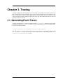
3. Tracing .................................................................................................................. 7
3.1. Generating Event Traces ................................................................................. 7
4. Analyzing Parallel Applications .................................................................................. 8
4.1. Text summary .............................................................................................. 8
4.2. ParaProf ...................................................................................................... 8
4.3. Jumpshot ..................................................................................................... 9
5. Quick Reference .................................................................................................... 10
6. Some Common Application Scenario ........................................................................ 11
6.1. Q. What routines account for the most time? How much? .................................... 11
6.2. Q. What loops account for the most time? How much? ....................................... 11
6.3. Q. What MFlops am I getting in all loops? ....................................................... 12
6.4. Q. Who calls MPI_Barrier() Where? ............................................................... 13
6.5. Q. How do I instrument Python Code? ............................................................ 14
6.6. Q. What happens in my code at a given time? ................................................... 14
6.7. Q. How does my application scale? ................................................................. 15
iv
List of Figures
4.1. Main Data Window ............................................................................................... 8
4.2. Main Data Window ............................................................................................... 9
6.1. Flat Profile ......................................................................................................... 11
6.2. Flat Profile with Loops ......................................................................................... 11
6.3. MFlops per loop .................................................................................................. 12
6.4. Callpath Profile ................................................................................................... 13
6.5. Tracing with Vampir ............................................................................................ 14
6.6. Scalability chart .................................................................................................. 15
2.1. ParaProf Manager Window ..................................................................................... 8
2.2. Loading Profile Data .............................................................................................. 8
2.3. Creating Derived Metrics ........................................................................................ 9
2.4. Main Data Window ............................................................................................. 10
2.5. Unstacked Bars ................................................................................................... 10
3.1. Triangle Mesh Plot .............................................................................................. 11
3.2. 3-D Mesh Plot .................................................................................................... 11
3.3. 3-D Scatter Plot .................................................................................................. 12
3.4. 3-D Scatter Plot .................................................................................................. 12
4.1. Thread Bar Graph ................................................................................................ 14
4.2. Thread Statistics Text Window .............................................................................. 14
4.3. Thread Statistics Table, inclusive and exclusive ........................................................ 15
4.4. Thread Statistics Table ......................................................................................... 15
4.5. Thread Statistics Table ......................................................................................... 16
4.6. Call Graph Window ............................................................................................. 16
4.7. Thread Call Path Relations Window ........................................................................ 17
4.8. User Event Statistics Window ................................................................................ 18
4.9. User Event Thread Bar Chart Window .................................................................... 18
5.1. Function Bar Graph ............................................................................................. 20
5.2. Function Histogram ............................................................................................. 20
6.1. Initial Phase Display ............................................................................................ 22
6.2. Phase Ledger ...................................................................................................... 22
6.3. Function Data over Phases .................................................................................... 23
7.1. Comparison Window (initial) ................................................................................ 24
7.2. Comparison Window (2 trials) ............................................................................... 24
7.3. Comparison Window (3 threads) ............................................................................ 25
8.1. User Event Bar Graph .......................................................................................... 26
8.2. Function Ledger .................................................................................................. 26
8.3. Group Ledger ..................................................................................................... 27
8.4. User Event Ledger ............................................................................................... 27
8.5. Selective Instrumentation Dialog ............................................................................ 28
9.1. ParaProf Preferences Window ............................................................................... 29
9.2. Edit Default Colors .............................................................................................. 30
9.3. Color Map ......................................................................................................... 30
4.1. Selecting a dimension reduction method .................................................................... 9
4.2. Entering a minimum threshold for exclusive percentage ................................................ 9
4.3. Entering a maximum number of clusters .................................................................. 10
4.4. Selecting a Metric to Cluster .................................................................................. 10
4.5. Confirm Clustering Options .................................................................................. 10
4.6. Cluster Results .................................................................................................... 11
4.7. Cluster Membership Histogram .............................................................................. 11
4.8. Cluster Membership Scatterplot ............................................................................. 12
4.9. Cluster Virtual Topology ...................................................................................... 13
4.10. Cluster Average Behavior ................................................................................... 14
5.1. Selecting a dimension reduction method .................................................................. 16
v
TAU User Guide
5.2. Entering a minimum threshold for exclusive percentage .............................................. 16
5.3. Selecting a Metric to Cluster .................................................................................. 16
5.4. Correlation Results .............................................................................................. 17
5.5. Correlation Example ............................................................................................ 18
6.1. Setting Group of Interest ....................................................................................... 20
6.2. Setting Metric of Interest ...................................................................................... 20
6.3. Setting Event of Interest ....................................................................................... 20
6.4. Setting Timesteps ................................................................................................ 21
6.5. Timesteps per Second .......................................................................................... 21
6.6. Relative Efficiency .............................................................................................. 22
6.7. Relative Efficiency by Event ................................................................................. 23
6.8. Relative Efficiency one Event ................................................................................ 23
6.9. Relative Speedup ................................................................................................ 24
6.10. Relative Speedup by Event .................................................................................. 24
6.11. Relative Speedup one Event ................................................................................ 25
6.12. Group % of Total Runtime .................................................................................. 26
6.13. Runtime Breakdown .......................................................................................... 26
6.14. Relative Efficiency per Phase ............................................................................... 27
6.15. Relative Speedup per Phase ................................................................................. 27
6.16. Phase Fraction of Total Runtime ........................................................................... 28
7.1. The Custom Charts Interface ................................................................................. 29
8.1. 3D Visualization of multivariate data ...................................................................... 31
8.2. Data Summary Window ....................................................................................... 32
8.3. Boxchart ............................................................................................................ 32
8.4. Histogram .......................................................................................................... 33
8.5. Normal Probability .............................................................................................. 34
9.1. Potential scalability data organized as a parametric study ............................................ 36
9.2. Selecting a table .................................................................................................. 36
9.3. Selecting a column .............................................................................................. 37
9.4. Selecting an operator ............................................................................................ 37
9.5. Selecting a value ................................................................................................. 37
9.6. Entering a name for the view ................................................................................. 37
9.7. The completed view ............................................................................................. 38
9.8. Selecting the base view ........................................................................................ 38
9.9. Completed sub-views ........................................................................................... 39
vi
List of Tables
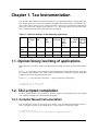
1.1. Different methods of instrumenting applications .......................................................... 1
vii
TAU Performance System® is a portable profiling and tracing toolkit for performance analysis of parallel programs written in Fortran, C, C++, Java, and Python. TAU (Tuning and Analysis Utilities) is capable of gathering performance information through instrumentation of functions, methods, basic blocks,
and statements. The TAU API also provides selection of profiling groups for organizing and controlling
instrumentation. Calls to the TAU API are made by probes inserted into the execution of the application
via source transformation, compiler directives or by library interposition.
This guide is organized into different sections. Readers wanting to get started right way can skip to the
Common Profile Requests section for step-by-step instructions for obtaining difference kinds of performance data. Or browse the starters guide for a quick reference to common TAU commands and variables.
TAU can be found on the web at: http://tau.uoregon.edu
viii
Chapter 1. Tau Instrumentation
TAU provides three methods to track the performance of your application. Binary rewriting using Dyninst, compiler directives or source transformation using PDT. Most projects need a comprehensive picture of where time is spent. The TAU Compiler provides a simple way to automatically instrument an
entire project. The TAU Compiler can be used on C, C++, fixed form Fortran, and free form Fortran.
Here is a table that lists the features/requirement for each method:
Table 1.1. Different methods of instrumenting applications
Method
Requires
recompiling
Requires
PDT
Binary rewriting
Shows
MPI
events
RoutineLow level Throttling Ability to
level event events
to reduce exclude file
(loops,
overhead from
inphases,
strumentaetc...)
tion
Yes
Compiler
Yes
Source
Yes
Yes
Yes
Yes
Yes
Yes
Yes
Yes
Yes
Yes
Yes
Yes
Yes
1.1. Dyninst binary rewriting of applications
This section will cover how to profile your application by rewriting your binary to inserted instrumentation.
The tau_run script allows you to instrument an application binary using the Dyninst Tool. (TAU must
be configured with Dyninst.) This feature allows instrumentation of already compiled executables
without TAU having to edit the application's code.
To use tau_run select the binary and use the -o option to name the rewritten binary:
%> tau_run -o a.inst a.out
%> mpirun -np 4 ./a.inst
1.2. TAU scripted compilation
For more detailed profiles, TAU provides two means to compile your application with TAU: through
your compiler or through source transformation using PDT.
1.2.1. Compiler Based Instrumentation
TAU provides these scripts: tau_f90.sh, tau_cc.sh, and tau_cxx.sh to instrument and compile Fortran, C,
and C++ programs respectively. You might use tau_cc.sh to compile a C program by typing:
%> module load tau
%> tau_cc.sh -tau_options=-optCompInst samplecprogram.c
1
Tau Instrumentation
On machines where a TAU module is not available, you will need to set the tau makefile and/or options.
The makefile and options controls how will TAU will compile you application. Use
%>tau_cc.sh -tau_makefile=[path to makefile] \
-tau_options=[option] samplecprogram.c
The Makefile can be found in the /[arch]/lib directory of your TAU distribution, for example /
x86_64/lib/Makefile.tau-mpi-pdt.
You can also use a Makefile specified in an environment variable. To run tau_cc.sh so it uses the Makefile specified by environment variable TAU_MAKEFILE, type:
%>export TAU_MAKEFILE=[path to tau]/[arch]/lib/[makefile]
%>export TAU_OPTIONS=-optCompInst
%>tau_cc.sh sampleCprogram.c
Similarly, if you want to set compile time options like selective instrumentation you can use the
TAU_OPTIONS environment variable.
1.2.2. Source Based Instrumentation
TAU provides these scripts: tau_f90.sh, tau_cc.sh, and tau_cxx.sh to instrument and compile Fortran, C,
and C++ programs respectively. You might use tau_cc.sh to compile a C program by typing:
%> module load tau
%> tau_cc.sh samplecprogram.c
When setting the TAU_MAKEFILE make sure the Makefile name contains pdt because you will need
a version of TAU built with PDT.
A list of options for the TAU compiler scripts can be found by typing man tau_compiler.sh or in
this chapter of the reference guide.
1.2.3. Options to TAU compiler scripts
These are some commonly used options available to the TAU compiler scripts. Either set them via the
TAU_OPTIONS environment variable or the -tau_options= option to tau_f90.sh,
tau_cc.sh, or tau_cxx.sh
-optVerbose
Enable verbose output (default: on)
-optKeepFiles
Do not remove intermediate files
-optShared
Use shared library of TAU
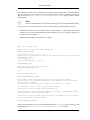
1.3. Selectively Profiling an Application
1.3.1. Custom Profiling
TAU allows you to customize the instrumentation of a program by using a selective instrumentation file.
2
Tau Instrumentation
This instrumentation file is used to manually control which parts of the application are profiled and how
they are profiled. If you are using one of the TAU compiler wrapper scripts to instrument your application you can use the -tau_options=-optTauSelectFile=<file> option to enable selective
instrumentation.
Note
Selective instrumentation is only available when using source-level instrumentation (PDT).
To specify a selective instrumentation file, create a text file and use the following guide to fill it in:
•
Wildcards for routine names are specified with the # mark (because * symbols show up in routine
signatures.) The # mark is unfortunately the comment character as well, so to specify a leading wildcard, place the entry in quotes.
•
Wildcards for file names are specified with * symbols.
Here is a example file:
#Tell tau to not profile these functions
BEGIN_EXCLUDE_LIST
void quicksort(int *, int, int)
# The next line excludes all functions beginning with "sort_" and having
# arguments "int *"
void sort_#(int *)
void interchange(int *, int *)
END_EXCLUDE_LIST
#Exclude these files from profiling
BEGIN_FILE_EXCLUDE_LIST
*.so
END_FILE_EXCLUDE_LIST
BEGIN_INSTRUMENT_SECTION
# A dynamic phase will break up the profile into phase where
# each events is recorded according to what phase of the application
# in which it occured.
dynamic phase name="foo1_bar" file="foo.c" line=26 to line=27
# instrument all the outer loops in this routine
loops file="loop_test.cpp" routine="multiply"
# tracks memory allocations/deallocations as well as potential leaks
memory file="foo.f90" routine="INIT"
# tracks the size of read, write and print statements in this routine
io file="foo.f90" routine="RINB"
END_INSTRUMENT_SECTION
Selective instrumentation files can be created automatically from ParaProf by right clicking on a trial
and selecting the FCreate Selective Instrumentation File menu item.
3
Chapter 2. Profiling
This chapter describes running an instrumented application, generating profile data and analyzing that
data. Profiling shows the summary statistics of performance metrics that characterize application performance behavior. Examples of performance metrics are the CPU time associated with a routine, the
count of the secondary data cache misses associated with a group of statements, the number of times a
routine executes, etc.
2.1. Running the Application
After instrumentation and compilation are completed, the profiled application is run to generate the profile data files. These files can be stored in a directory specified by the environment variable PROFILEDIR. By default, profiles are placed in the current directory. You can also set the TAU_VERBOSE
enviroment variable to see the steps the TAU measurement systems takes when your application is running. Example:
% setenv TAU_VERBOSE 1
% setenv PROFILEDIR /home/sameer/profiledata/experiment55
% mpirun -np 4 matrix
Other environment variables you can set to enable these advanced MPI measurement features are
TAU_TRACK_MESSAGE to track MPI message statistics when profiling or messages lines when tracing,
and TAU_COMM_MATRIX to generate MPI communication matrix data.
2.2. Reducing Performance Overhead with
TAU_THROTTLE
TAU automatically throttles short running functions in an effort to reduce the amount of overhead associated with profiles of such functions. This feature may be turned off by setting the environment variable
TAU_THROTTLE to 0. The default rules TAU uses to determine which functions to throttle is: numcalls > 100000 && usecs/call < 10 which means that if a function executes more than
100000 times and has an inclusive time per call of less than 10 microseconds, then profiling of that function will be disabled after that threshold is reached. To change the values of numcalls and usecs/call the
user may optionally set environment variables:
% setenv TAU_THROTTLE_NUMCALLS 2000000
% setenv TAU_THROTTLE_PERCALL 5
The changes the values to 2 million and 5 microseconds per call. Functions that are throttled are marked
explicitly in there names as THROTTLED.
2.3. Profiling each event callpath
You can enable callpath profiling by setting the environment variable TAU_CALLPATH. In this mode
TAU will recorded the each event callpath to the depth set by the TAU_CALLPATH_DEPTH environment variable (default is two). Because instrumentation overhead will increase with the depth of the callpath, you should use the shortest call path that is sufficient.
4
Profiling
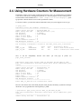
2.4. Using Hardware Counters for Measurement
Performance counters exist on many modern microprocessors. They can count hardware performance
events such as cache misses, floating point operations, etc. while the program executes on the processor.
The Performance Data Standard and API (PAPI [http://icl.cs.utk.edu/papi/]) package provides a uniform interface to access these performance counters.
To use these counters, you must first find out which PAPI events your system supports. To do so type:
%> papi_avail
Available events and hardware information.
------------------------------------------------------------------------Vendor string and code
: AuthenticAMD (2)
Model string and code
: AMD K8 Revision C (15)
CPU Revision
: 2.000000
CPU Megahertz
: 2592.695068
CPU's in this Node
: 4
Nodes in this System
: 1
Total CPU's
: 4
Number Hardware Counters : 4
Max Multiplex Counters
: 32
------------------------------------------------------------------------The following correspond to fields in the PAPI_event_info_t structure.
Name
PAPI_L1_DCM
PAPI_L1_ICM
...
Code
0x80000000
0x80000001
Next, to test the compatibility
papi_event_chooser:
Avail
Yes
Yes
between
each
Deriv
Yes
Yes
metric
you
Description (Note)
Level 1 data cache misses
Level 1 instruction cache misses
wish
papi
to
profile,
use
papi/utils> papi_event_chooser PAPI_LD_INS PAPI_SR_INS PAPI_L1_DCM
Test case eventChooser: Available events which can be added with given
events.
------------------------------------------Vendor string and code
: GenuineIntel (1)
Model string and code
: Itanium 2 (2)
CPU Revision
: 1.000000
CPU Megahertz
: 1500.000000
CPU's in this Node
: 16
Nodes in this System
: 1
Total CPU's
: 16
Number Hardware Counters : 4
Max Multiplex Counters
: 32
------------------------------------------Event PAPI_L1_DCM can't be counted with others
Here the event chooser tells us that PAPI_LD_INS, PAPI_SR_INS, and PAPI_L1_DCM are incompatible metrics. Let try again this time removing PAPI_L1_DCM:
% papi/utils> papi_event_chooser PAPI_LD_INS PAPI_SR_INS
Test case eventChooser: Available events which can be added with given
events.
------------------------------------------Vendor string and code
: GenuineIntel (1)
5
Profiling
Model string and code
: Itanium 2 (2)
CPU Revision
: 1.000000
CPU Megahertz
: 1500.000000
CPU's in this Node
: 16
Nodes in this System
: 1
Total CPU's
: 16
Number Hardware Counters : 4
Max Multiplex Counters
: 32
------------------------------------------Usage: eventChooser NATIVE|PRESET evt1 evet2 ...
Here the event chooser verifies that PAPI_LD_INS and PAPI_SR_INS are compatible metrics.
Next, make sure that you are using a makefile with papi in its name. Then set the environment variable
TAU_METRICS to a colon delimited list of PAPI metrics you would like to use.
setenv TAU_METRICS PAPI_FP_OPS\:PAPI_L1_DCM
In addition to PAPI counters, we support TIME (via unix gettimeofday). On Linux and CrayCNL systems, we provide the high resolution LINUXTIMERS metric and on BGL/BGP systems we provide
BGLTIMERS and BGPTIMERS.
6
Chapter 3. Tracing
Typically, profiling shows the distribution of execution time across routines. It can show the code locations associated with specific bottlenecks, but it can not show the temporal aspect of performance variations. Tracing the execution of a parallel program shows when and where an event occurred, in terms
of the process that executed it and the location in the source code. This chapter discusses how TAU can
be used to generate event traces.
3.1. Generating Event Traces
To enable tracing with TAU, set the environment variable TAU_TRACE to 1. Similarly you can enable/
disable profile with the TAU_PROFILE variable. Just like with profiling, you can set the output directory with a environment variable:
% setenv TRACEDIR /users/sameer/tracedata/experiment56
This will generate a trace file and an event file for each processor. To merge these files, use the
tau_treemerge.pl script. If you want to convert TAU trace file into another format use the
tau2otf, tau2vtf, or tau2slog2 scripts.
7
Chapter 4. Analyzing Parallel
Applications
4.1. Text summary
For a quick view summary of TAU performance, use pprof It reads and prints a summary of the TAU
data in the current directory. For performance data with multiple metrics, move into one of the directories to get information about that metric:
%> cd MULTI__P_WALL_CLOCK_TIME
%> pprof
Reading Profile files in profile.*
NODE 0;CONTEXT 0;THREAD 0:
----------------------------------------------------------------------------------%Time
Exclusive
Inclusive
#Call
#Subrs Inclusive Name
msec
total msec
usec/call
----------------------------------------------------------------------------------100.0
24
590
1
1
590963 main
95.9
26
566
1
2
566911 multiply
47.3
279
279
1
0
279280 multiply-opt
44.1
260
260
1
0
260860 multiply-regular
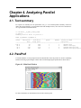
4.2. ParaProf
To launch ParaProf, execute paraprof from the command line where the profiles are located. Launching
ParaProf will bring up the manager window and a window displaying the profile data as shown below.
Figure 4.1. Main Data Window
For more information see the ParaProf section in the reference guide.
8
Analyzing Parallel Applications
4.3. Jumpshot
To use Argonne's Jumpshot (bundled with TAU), first merge and convert TAU traces to slog2 format:
% tau_treemerge.pl
% tau2slog2 tau.trc tau.edf -o tau.slog2
% jumpshot tau.slog2
Launching Jumpshot will bring up the main display window showing the entire trace, zoom in to see
more detail.
Figure 4.2. Main Data Window
9
Chapter 5. Quick Reference
tau_run
TAU's binary instrumentation tool
tau_cc.sh
-tau_options=-optCompInst
/
tau_cxx.sh
tau_options=-optCompInst / tau_f90.sh -tau_options=-optCompInst
Compiler wrappers (Compiler instrumentation)
-
tau_cc.sh / tau_cxx.sh / tau_f90.sh
Compiler wrappers (PDT instrumentation)
TAU_MAKEFILE
Set instrumentation definition file
TAU_OPTIONS
Set instrumentation options
dynamic
phase
name='name'
line=end_line_#
Specify dynamic Phase
file='filename'
line=start_line_#
loops file='filename' routine='routine name'
Instrument outer loops
memory file='filename' routine='routine name'
Track memory
io file='filename' routine='routine name'
Track IO
TAU_PROFILE / TAU_TRACE
Enable profiling and/or tracing
PROFILEDIR / TRACEDIR
Set profile/trace output directory
TAU_CALLPATH=1 / TAU_CALLPATH_DEPTH
Enable Callpath profiling, set callpath depth
TAU_THROTTLE=1 / TAU_THROTTLE_NUMCALLS / TAU_THROTTLE_PERCALL
Enable event throttling, set number of call, percall (us) threshold
TAU_METRICS
List of PAPI metrics to profile
tau_treemerge.pl
Merge traces to one file
tau2otf / tau2vtf / tau2slog2
Trace conversion tools
10
to
Chapter 6. Some Common Application
Scenario
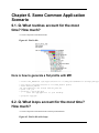
6.1. Q. What routines account for the most
time? How much?
A. Create a flat profile with wallclock time.
Figure 6.1. Flat Profile
Here is how to generate a flat profile with MPI
% setenv TAU_MAKEFILE /opt/apps/tau/tau-2.17.1/x86_64/lib/Makefile.tau-mpi-pdt-pgi
% set path=(/opt/apps/tau/tau-2.17.1/x86_64/bin $path)
% make F90=tau_f90.sh
(Or edit Makefile and change F90=tau_f90.sh)
% qsub run.job
% paraprof -–pack app.ppk
Move the app.ppk file to your desktop.
% paraprof app.ppk
6.2. Q. What loops account for the most time?
How much?
A. Create a flat profile with wallclock time with loop instrumentation.
Figure 6.2. Flat Profile with Loops
11
Some Common Application Scenario
Here is how to instrument loops in an application
% setenv TAU_MAKEFILE /opt/apps/tau/tau-2.17.1/x86_64/lib/Makefile.tau-mpi-pdt
% setenv TAU_OPTIONS ‘-optTauSelectFile=select.tau –optVerbose’
% cat select.tau
BEGIN_INSTRUMENT_SECTION
loops routine=“#”
END_INSTRUMENT_SECTION
% set path=(/opt/apps/tau/tau-2.17.1/x86_64/bin $path)
% make F90=tau_f90.sh
(Or edit Makefile and change F90=tau_f90.sh)
% qsub run.job
% paraprof -–pack app.ppk
Move the app.ppk file to your desktop.
% paraprof app.ppk
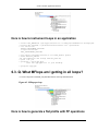
6.3. Q. What MFlops am I getting in all loops?
A. Create a flat profile with PAPI_FP_INS/OPS and time with loop instrumentation.
Figure 6.3. MFlops per loop
Here is how to generate a flat profile with FP operations
12
Some Common Application Scenario
% setenv TAU_MAKEFILE /opt/apps/tau/tau-2.17.1/x86_64/lib/Makefile.tau-papi-mpi-pdt
% setenv TAU_OPTIONS ‘-optTauSelectFile=select.tau –optVerbose’
% cat select.tau
BEGIN_INSTRUMENT_SECTION
loops routine=“#”
END_INSTRUMENT_SECTION
% set path=(/opt/apps/tau/tau-2.17.1/x86_64/bin $path)
% make F90=tau_f90.sh
(Or edit Makefile and change F90=tau_f90.sh)
% setenv TAU_METRICS GET_TIME_OF_DAY\:PAPI_FP_INS
% qsub run.job
% paraprof -–pack app.ppk
Move the app.ppk file to your desktop.
% paraprof app.ppk
Choose 'Options' -> 'Show Derived Panel' -> Arg 1 = PAPI_FP_INS, Arg 2 =
GET_TIME_OF_DAY, Operation = Divide -> Apply, close.
6.4. Q. Who calls MPI_Barrier() Where?
A. Create a callpath profile with given depth.
Figure 6.4. Callpath Profile
Here is how to generate a callpath profile with MPI
% setenv TAU_MAKEFILE
% /opt/apps/tau/tau-2.17.1/x86_64/lib/Makefile.tau-mpi-pdt
% set path=(/opt/apps/tau/tau-2.17.1/x86_64/bin $path)
% make F90=tau_f90.sh
(Or edit Makefile and change F90=tau_f90.sh)
13
Some Common Application Scenario
% setenv TAU_CALLPATH 1
% setenv TAU_CALLPATH_DEPTH 100
% qsub run.job
% paraprof -–pack app.ppk
Move the app.ppk file to your desktop.
% paraprof app.ppk
(Windows -> Thread -> Call Graph)
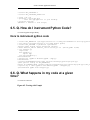
6.5. Q. How do I instrument Python Code?
A. Create an python wrapper library.
Here to instrument python code
% setenv TAU_MAKEFILE /opt/apps/tau/tau-2.17.1/x86_64/lib/Makefile.tau-icpc-python% set path=(/opt/apps/tau/tau-2.17.1/x86_64/bin $path)
% setenv TAU_OPTIONS ‘-optShared -optVerbose'
(Python needs shared object based TAU library)
% make F90=tau_f90.sh CXX=tau_cxx.sh CC=tau_cc.sh (build pyMPI w/TAU)
% cat wrapper.py
import tau
def OurMain():
import App
tau.run(‘OurMain()’)
Uninstrumented:
% mpirun.lsf /pyMPI-2.4b4/bin/pyMPI ./App.py
Instrumented:
% setenv PYTHONPATH<taudir>/x86_64/<lib>/bindings-python-mpi-pdt-pgi
(same options string as TAU_MAKEFILE)
setenv LD_LIBRARY_PATH <taudir>/x86_64/lib/bindings-icpc-python-mpi-pdt-pgi\:$LD_LI
% mpirun –np 4 <dir>/pyMPI-2.4b4-TAU/bin/pyMPI ./wrapper.py
(Instrumented pyMPI with wrapper.py)
6.6. Q. What happens in my code at a given
time?
A. Create an event trace.
Figure 6.5. Tracing with Vampir
14
Some Common Application Scenario
How to create a trace
% setenv TAU_MAKEFILE
% /opt/apps/tau/tau-2.17.1/x86_64/lib/Makefile.tau-mpi-pdt-pgi
% set path=(/opt/apps/tau/tau-2.17.1/x86_64/bin $path)
% make F90=tau_f90.sh
(Or edit Makefile and change F90=tau_f90.sh)
% setenv TAU_TRACE 1
% qsub run.job
% tau_treemerge.pl
(merges binary traces to create tau.trc and tau.edf files)
JUMPSHOT:
% tau2slog2 tau.trc tau.edf –o app.slog2
% jumpshot app.slog2
OR
VAMPIR:
% tau2otf tau.trc tau.edf app.otf –n 4 –z
(4 streams, compressed output trace)
% vampir app.otf
(or vng client with vngd server).
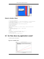
6.7. Q. How does my application scale?
A. Examine profiles in PerfExplorer.
Figure 6.6. Scalability chart
15
Some Common Application Scenario
How to examine a series of profiles in PerfExplorer
% setenv TAU_MAKEFILE /opt/apps/tau/tau-2.17.1/x86_64/lib/Makefile.tau-mpi-pdt
% set path=(/opt/apps/tau/tau-2.17.1/x86_64/bin $path)
% make F90=tau_f90.sh
(Or edit Makefile and change F90=tau_f90.sh)
% qsub run1p.job
% paraprof -–pack 1p.ppk
% qsub run2p.job
% paraprof -–pack 2p.ppk ...and so on.
On your client:
% perfdmf_configure
(Choose derby, blank user/password, yes to save password, defaults)
% perfexplorer_configure
(Yes to load schema, defaults)
% paraprof
(load each trial: Right click on trial ->Upload trial to DB
% perfexplorer
(Charts -> Speedup)
16
ParaProf - User's Manual
University of Oregon
ParaProf - User's Manual
by University of Oregon
Published (TBA)
Copyright © 2005-2010 University of Oregon Performance Research Lab
Table of Contents
1. Introduction ............................................................................................................ 6
1.1. Using ParaProf from the command line ..................................................... 6
1.2. Supported Formats ................................................................................ 6
1.3. Command line options ........................................................................... 7
2. Profile Data Management .......................................................................................... 8
2.1. ParaProf Manager Window ..................................................................... 8
2.2. Loading Profiles .................................................................................... 8
2.3. Database Interaction .............................................................................. 9
2.4. Creating Derived Metrics ........................................................................ 9
2.5. Main Data Window ............................................................................... 9
3. 3-D Visualization ................................................................................................... 11
3.1. Triangle Mesh Plot .............................................................................. 11
3.2. 3-D Bar Plot ....................................................................................... 11
3.3. 3-D Scatter Plot .................................................................................. 12
3.4. 3-D Scatter Plot .................................................................................. 12
4. Thread Based Displays ........................................................................................... 14
4.1. Thread Bar Graph ................................................................................ 14
4.2. Thread Statistics Text Window .............................................................. 14
4.3. Thread Statistics Table ......................................................................... 15
4.4. Call Graph Window ............................................................................. 16
4.5. Thread Call Path Relations Window ........................................................ 17
4.6. User Event Statistics Window ................................................................ 18
4.7. User Event Thread Bar Chart ................................................................. 18
5. Function Based Displays ......................................................................................... 20
5.1. Function Bar Graph ............................................................................. 20
5.2. Function Histogram ............................................................................. 20
6. Phase Based Displays ............................................................................................. 22
6.1. Using Phase Based Displays .................................................................. 22
7. Comparative Analysis ............................................................................................. 24
7.1. Using Comparitive Analysis .................................................................. 24
8. Miscellaneous Displays ........................................................................................... 26
8.1. User Event Bar Graph .......................................................................... 26
8.2. Ledgers ............................................................................................. 26
8.2.1. Function Ledger ....................................................................... 26
8.2.2. Group Ledger ........................................................................... 27
8.2.3. User Event Ledger .................................................................... 27
8.3. Selective Instrumentation File Generator ................................................. 28
9. Preferences ........................................................................................................... 29
9.1. Preferences Window ............................................................................ 29
9.2. Default Colors .................................................................................... 30
9.3. Color Map ......................................................................................... 30
iv
List of Figures
2.1. ParaProf Manager Window ..................................................................................... 8
2.2. Loading Profile Data .............................................................................................. 8
2.3. Creating Derived Metrics ........................................................................................ 9
2.4. Main Data Window ............................................................................................. 10
2.5. Unstacked Bars ................................................................................................... 10
3.1. Triangle Mesh Plot .............................................................................................. 11
3.2. 3-D Mesh Plot .................................................................................................... 11
3.3. 3-D Scatter Plot .................................................................................................. 12
3.4. 3-D Scatter Plot .................................................................................................. 12
4.1. Thread Bar Graph ................................................................................................ 14
4.2. Thread Statistics Text Window .............................................................................. 14
4.3. Thread Statistics Table, inclusive and exclusive ........................................................ 15
4.4. Thread Statistics Table ......................................................................................... 15
4.5. Thread Statistics Table ......................................................................................... 16
4.6. Call Graph Window ............................................................................................. 16
4.7. Thread Call Path Relations Window ........................................................................ 17
4.8. User Event Statistics Window ................................................................................ 18
4.9. User Event Thread Bar Chart Window .................................................................... 18
5.1. Function Bar Graph ............................................................................................. 20
5.2. Function Histogram ............................................................................................. 20
6.1. Initial Phase Display ............................................................................................ 22
6.2. Phase Ledger ...................................................................................................... 22
6.3. Function Data over Phases .................................................................................... 23
7.1. Comparison Window (initial) ................................................................................ 24
7.2. Comparison Window (2 trials) ............................................................................... 24
7.3. Comparison Window (3 threads) ............................................................................ 25
8.1. User Event Bar Graph .......................................................................................... 26
8.2. Function Ledger .................................................................................................. 26
8.3. Group Ledger ..................................................................................................... 27
8.4. User Event Ledger ............................................................................................... 27
8.5. Selective Instrumentation Dialog ............................................................................ 28
9.1. ParaProf Preferences Window ............................................................................... 29
9.2. Edit Default Colors .............................................................................................. 30
9.3. Color Map ......................................................................................................... 30
v
Chapter 1. Introduction
ParaProf is a portable, scalable performance analysis tool included with the TAU distribution.
Important
ParaProf requires Sun's Java 1.3 Runtime Environment for basic functionality. Java 1.4 is
required for 3d visualization and image export. Additionally, OpenGL is required for 3d
visualization.
Note
Most windows in ParaProf can export bitmap (png/jpg) and vector (svg/eps) images to disk
(png/jpg) or print directly to a printer. This are available through the File menu.
1.1. Using ParaProf from the command line
ParaProf is a java program that is run from the supplied paraprof script (paraprof.bat for windows binary release).
% paraprof --help
Usage: paraprof [options] <files/directory>
Options:
-f, --filetype <filetype>
-h, --help
-p
-i, --fixnames
-m, --monitor
Specify type of performance data,
options are: profiles (default), pprof,
dynaprof, mpip, gprof, psrun, hpm,
packed, cube, hpc, ompp
Display this help message
Use `pprof` to compute derived data
Use the fixnames option for gprof
Perform runtime monitoring of profile data
The following options will run only from the console (no GUI will launch):
--pack <file>
--dump
-o, --oss
-s, --summary
Pack the data into packed (.ppk) format
Dump profile data to TAU profile format
Print profile data in OSS style text output
Print only summary statistics
(only applies to OSS output)
Notes:
For the TAU profiles type, you can specify either a specific set of
profile files on the commandline, or you can specify a directory
(by default the current directory). The specified directory will
be searched for profile.*.*.* files, or, in the case of
multiple counters, directories named MULTI_* containing profile data.
1.2. Supported Formats
ParaProf can load profile date from many sources. The types currently supported are:
6
Introduction
•
TAU Profiles - Output from the TAU measurement library, these files generally take the form of
profile.X.X.X, one for each node/context/thread combination. When multiple counters are
used, each metric is located in a directory prefixed with "MULTI__". To launch ParaProf with all the
metrics, simply launch it from the root of the MULTI__ directories.
•
pprof - Dump Output from TAU's pprof -d. Provided for backward compatibility only.
•
DynaProf - Output From DynaProf's wallclock and papi probes.
•
mpiP - Output from mpiP.
•
gprof - Output from gprof, see also the --fixnames option.
•
HPM Toolkit - Output from HPM Toolkit.
•
ParaProf Packed Format - Export format supported by PerfDMF/ParaProf. Typically .ppk.
•
Cube - Output from Kojak Expert tool for use with Cube.
•
HPCToolkit - XML data from hpcquick. Typically, the user runs hpcrun, then hpcquick on the resulting binary file.
•
ompP - CSV format from the ompP OpenMP Profiler (http://www.ompp-tool.com). The user must
use OMPP_OUTFORMAT=CVS.
1.3. Command line options
In addition to specifying the profile format, the user can also specify the following options
•
--fixnames - Use the fixnames option for gprof. When C and Fortran code are mixed, the C routines
have to be mapped to either .function or function_. Strip the leading period or trailing underscore, if
it is there.
•
--pack <file> - Rather than load the data and launch the GUI, pack the data into the specified file.
•
--dump - Rather than load the data and launch the GUI, dump the data to TAU Profiles. This can be
used to convert supported formats to TAU Profiles.
•
--oss - Outputs profile data in OSS Style. Example:
------------------------------------------------------------------------------Thread: n,c,t 0,0,0
------------------------------------------------------------------------------excl.secs excl.%
cum.%
PAPI_TOT_CYC
PAPI_FP_OPS
calls function
0.005
56.0%
56.0%
13475345
4194518
1 foo
0.003
40.1%
96.1%
9682185
4205367
1 bar
0
3.6%
99.7%
223173
17445
1 baz
2.2E-05
0.3% 100.0%
14663
206
1 main
•
--summary - Output only summary information for OSS style output.
7
Chapter 2. Profile Data Management
ParaProf uses PerfDMF to manage profile data. This enables it to read the various profile formats as
well as store and retrieve them from a database.
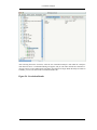
2.1. ParaProf Manager Window
Upon launching ParaProf, the user is greeted with the ParaProf Manager Window.
Figure 2.1. ParaProf Manager Window
This window is used to manage profile data. The user can upload/download profile data, edit meta-data,
launch visual displays, export data, derive new metrics, etc.
2.2. Loading Profiles
To load profile data, select File->Open, or right click on the Application's tree and select "Add Trial".
Figure 2.2. Loading Profile Data
8
Profile Data Management
Select the type of data from the "Trial Type" drop-down box. For TAU Profiles, select a directory, for
other types, files.
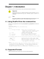
2.3. Database Interaction
Database interaction is done through the tree view of the ParaProf Manager Window. Applications expand to Experiments, Experiments to Trials, and Trials are loaded directly into ParaProf just as if they
were read off disk. Additionally, the meta-data associated with each element is show on the right, as in
Figure 2.1, “ParaProf Manager Window”. A trial can be exported by right clicking on it and selecting
"Export as Packed Profile".
New trials can be uploaded to the database by either right-clicking on an entity in the database and selecting "Add Trial", or by right-clicking on an Application/Experiment/Trial hierarchy from the "Standard Applications" and selecting "Upload Application/Experiment/Trial to DB".
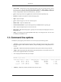
2.4. Creating Derived Metrics
ParaProf can created derived metrics using the Derived Metric Panel, available from the Options menu
of the ParaProf Manager Window.
Figure 2.3. Creating Derived Metrics
In Figure 2.3, “Creating Derived Metrics”, we have just divided Floating Point Instructions by Wallclock time, creating FLOPS (Floating Point Operations per Second). The 2nd argument is a user editable
text-box and can be filled in with scalar values by using the keyword 'val' (e.g. "val 1.5").
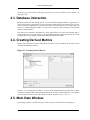
2.5. Main Data Window
Upon loading a profile, or double-clicking on a metric, the Main Data Window will be displayed.
9
Profile Data Management
Figure 2.4. Main Data Window
This window shows each thread as well as statistics as a combined bar graph. Each function is represented by a different color (though possibly cycled). From anywhere in ParaProf, you can right-click on objects representing threads or functions to launch displays associated with those objects. For example, in
Figure 2.4, “Main Data Window”, right click on the text n,c,t, 8,0,0 to launch thread based displays for
node 8.
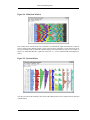
Figure 2.5. Unstacked Bars
You may also turn off the stacking of bars so that individual functions can be compared across threads in
a global display.
10
Chapter 3. 3-D Visualization
ParaProf displays massive parallel profiles through the use of OpenGL hardware acceleration through
the 3D Visualization window. Each window is fully configurable with rotation, translation, and zooming
capabilities. Rotation is accomplished by holding the left mouse button down and dragging the mouse.
Translation is done likewise with the right mouse button. Zooming is done with the mousewheel and the
+ and - keyboard buttons.
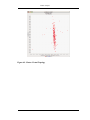
3.1. Triangle Mesh Plot
Figure 3.1. Triangle Mesh Plot
This visualization method shows two metrics for all functions, all threads. The height represents one
chosen metric, and the color, another. These are selected from the drop-down boxes on the right.
To pinpoint a specific value in the plot, move the Function and Thread sliders to cycle through the available functions/threads. The values for the two metrics, in this case for MPI_Recv() on Node 351,
the value is 14.37 seconds.
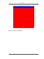
3.2. 3-D Bar Plot
Figure 3.2. 3-D Mesh Plot
11
3-D Visualization
This visualization method is similar to the triangle mesh plot. It simply displays the data using 3d bars
instead of a mesh. The controls works the same. Note that in Figure 3.2, “3-D Mesh Plot” the transparency option is selected, which changes the way in which the selection model operates.
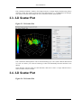
3.3. 3-D Scatter Plot
Figure 3.3. 3-D Scatter Plot
This visualization method plots the value of each thread along up to 4 axes (each a different function/metric). This view allows you to discern clustering of values and relationships between functions across
threads.
Select functions using the button for each dimension, then select a metric. A single function across 4
metrics could be used, for example.
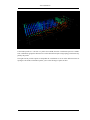
3.4. 3-D Scatter Plot
Figure 3.4. 3-D Scatter Plot
12
3-D Visualization
If the loaded profile is a cube file or a profile from a BGB, then this visualization option is available.
This visualizations groups the threads in two or three dimensional space using topology information supplied by the profile.
The right side bar provides options to manipulate the visualization. You can select different metrics or
topologies. The sliders toward the top allow you to select the range of points to show.
13
Chapter 4. Thread Based Displays
ParaProf displays several windows that show data for one thread of execution. In addition to per thread
values, the users may also select mean or standard deviation as the "thread" to display. In this mode, the
mean or standard deviation of the values across the threads will be used as the value.
4.1. Thread Bar Graph
Figure 4.1. Thread Bar Graph
This display graphs each function on a particular thread for comparison. The metric, units, and sort order
can be changed from the Options menu.
4.2. Thread Statistics Text Window
Figure 4.2. Thread Statistics Text Window
14
Thread Based Displays
This display shows a pprof style text view of the data.
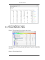
4.3. Thread Statistics Table
Figure 4.3. Thread Statistics Table, inclusive and exclusive
This display shows the callpath data in a table. Each callpath can be traced from root to leaf by opening
each node in the tree view. A colorscale immediately draws attention to "hot spots", areas that contain
highest values.
Figure 4.4. Thread Statistics Table
15
Thread Based Displays
Figure 4.5. Thread Statistics Table
The display can be used in one of two ways, in "inclusive/exclusive" mode, both the inclusive and exclusive values are shown for each path, see Figure 4.3, “Thread Statistics Table, inclusive and exclusive” for an example.
When this option is off, the inclusive value for a node is show when it is closed, and the exclusive value
is shown when it is open. This allows the user to more easily see where the time is spent since the total
time for the application will always be represented in one column. See Figure 4.4, “Thread Statistics Table” and Figure 4.5, “Thread Statistics Table” for examples. This display also functions as a regular statistics table without callpath data. The data can be sorted by columns by clicking on the column heading.
When multiple metrics are available, you can add and remove columns for the display using the menu.
4.4. Call Graph Window
Figure 4.6. Call Graph Window
16
Thread Based Displays
This display shows callpath data in a graph using two metrics, one determines the width, the other the
color. The full name of the function as well as the two values (color and width) are displayed in a tooltip
when hovering over a box. By clicking on a box, the actual ancestors and descendants for that function
and their paths (arrows) will be highlighted with blue. This allows you to see which functions are called
by which other functions since the interplay of multiple paths may obscure it.
4.5. Thread Call Path Relations Window
Figure 4.7. Thread Call Path Relations Window
17
Thread Based Displays
This display shows callpath data in a gprof style view. Each function is shown with its immediate parents. For example, Figure 4.7, “Thread Call Path Relations Window” shows that MPI_Recv() is call
from two places for a total of 9.052 seconds. Most of that time comes from the 30 calls when
MPI_Recv() is called by MPIScheduler::postMPIRecvs(). The other 60 calls do not amount
to much time.
4.6. User Event Statistics Window
Figure 4.8. User Event Statistics Window
This display shows a pprof style text view of the user event data. Right clicking on a User Event will
give you the option to open a Bar Graph for that particular User Event across all threads. See Section 8.1, “User Event Bar Graph”
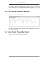
4.7. User Event Thread Bar Chart
Figure 4.9. User Event Thread Bar Chart Window
18
Thread Based Displays
This display shows a particular thread's user defined event statistics as a bar chart. This is the same data
from the Section 4.6, “User Event Statistics Window”, in graphical form.
19
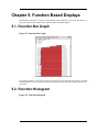
Chapter 5. Function Based Displays
ParaProf has two displays for showing a single function across all threads of execution. This chapter describes the Function Bar Graph Window and the Function Histogram Window.
5.1. Function Bar Graph
Figure 5.1. Function Bar Graph
This display graphs the values that the particular function had for each thread along with the mean and
standard deviation across the threads. You may also change the units and metric displayed from the Options menu.
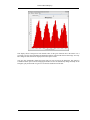
5.2. Function Histogram
Figure 5.2. Function Histogram
20
Function Based Displays
This display shows a histogram of each thread's value for the given function. Hover the mouse over a
given bar to see the range minimum and maximum and how many threads fell into that range. You may
also change the units and metric displayed from the Options menu.
You may also dynamically change how many bins are used (1-100) in the histogram. This option is
available from the Options menu. Changing the number of bins can dramatically change the shape of the
histogram, play around with it to get a feel for the true distribution of the data.
21
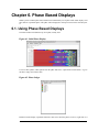
Chapter 6. Phase Based Displays
When a profile contains phase data, ParaProf will automatically run in phase mode. Most displays will
show data for a particular phase. This phase will be displayed in teh top left corner in the meta data panel.
6.1. Using Phase Based Displays
The initial window will default to top level phase, usually main
Figure 6.1. Initial Phase Display
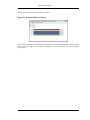
To access other phases, either right click on the phase and select, "Open Profile for this Phase", or go to
the Phase Ledger and select it there.
Figure 6.2. Phase Ledger
ParaProf can also display a particular function's value across all of the phases. To do so, right click on a
22
Phase Based Displays
function and select, "Show Function Data over Phases".
Figure 6.3. Function Data over Phases
Because Phase information is implemented as callpaths, many of the callpath displays will show phase
data as well. For example, the Call Path Text Window is useful for showing how functions behave
across phases.
23
Chapter 7. Comparative Analysis
ParaProf can perform cross-thread and cross-trial anaylsis. In this way, you can compare two or more
trials and/or threads in a single display.
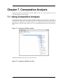
7.1. Using Comparitive Analysis
Comparative analysis in ParaProf is based on individual threads of execution. There is a maximum of
one Comparison window for a given ParaProf session. To add threads to the window, right click on
them and select "Add Thread to Comparison Window". The Comparison Window will pop up with the
thread selected. Note that "mean" and "std. dev." are considered threads for this any most other purposes.
Figure 7.1. Comparison Window (initial)
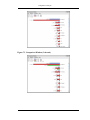
Add additional threads, from any trial, by the same means.
Figure 7.2. Comparison Window (2 trials)
24
Comparative Analysis
Figure 7.3. Comparison Window (3 threads)
25
Chapter 8. Miscellaneous Displays
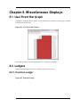
8.1. User Event Bar Graph
In addition to displaying the text statistics for User Defined Events, ParaProf can also graph a particular
User Event across all threads.
Figure 8.1. User Event Bar Graph
This display graphs the value that the particular user event had for each thread.
8.2. Ledgers
ParaProf has three ledgers that show the functions, groups, and user events.
8.2.1. Function Ledger
Figure 8.2. Function Ledger
26
Miscellaneous Displays
The function ledger shows each function along with its current color. As with other displays showing
functions, you may right-click on a function to launch other function-specific displays.
8.2.2. Group Ledger
Figure 8.3. Group Ledger
The group ledger shows each group along with its current color. This ledger is especially important because it gives you the ability to mask all of the other displays based on group membership. For example,
you can right-click on the MPI group and select "Show This Group Only" and all of the windows will
now mask to only those functions which are members of the MPI group. You may also mask by the inverse by selecting "Show All Groups Except This One" to mask out a particular group.
8.2.3. User Event Ledger
Figure 8.4. User Event Ledger
27
Miscellaneous Displays
The user event ledger shows each user event along with its current color.
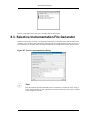
8.3. Selective Instrumentation File Generator
ParaProf can also help you refine your program performance by excluding some functions from instrumentation. You can select rules to determine which function get excluded; both rules must be true for a
given function to be excluded. Below each function that will be excluded based on these rules are listed.
Figure 8.5. Selective Instrumentation Dialog
Note
Only the functions profilied in ParaProf can be excluded. If you had previously setup selective instrumentation for this application the functions that where previously excluded
will not longer be excluded.
28
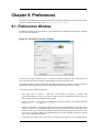
Chapter 9. Preferences
Preferences are modified from the ParaProf Preferences Window, launched from the File menu. Preferences are saved between sessions in the .ParaProf/ParaProf.prefs
9.1. Preferences Window
In addition to displaying the text statistics for User Defined Events, ParaProf can also graph a particular
User Event across all threads.
Figure 9.1. ParaProf Preferences Window
The preferences window allows the user to modify the behavior and display style of ParaProf's windows. The font size affects bar height, a sample display is shown in the upper-right.
The Window defaults section will determine the initial settings for new windows. You may change the
initial units selection and whether you want values displayed as percentages or as raw values.
The Settings section controls the following
•
Show Path Title in Reverse - Path title will normally be shown in normal order
(/home/amorris/data/etc). They can be reverse using this option (etc/data/amorris/home). This only
affects loaded trials and the titlebars of new windows.
•
Reverse Call Paths - This option will immediately change the display of all callpath functions
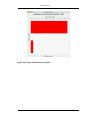
between Root => Leaf and Leaf <= Root.
•
Statistics Computation - Turning this option on causes the mean computation to take the sum of
value for a function across all threads and divide it by the total number of threads. With this option
off the sum will only be divided by the number of threads that actively participated in the sum. This
way the user can control whether or not threads which do not call a particular function are consider
as a 0 in the computation of statistics.
•
Generate Reverse Calltree Data - This option will enable the generation of reverse callpath data ne29
Preferences
cessary for the reverse callpath option of the statistics tree-table window.
•
Show Source Locations - This option will enable the display of source code locations in event
names.
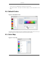
9.2. Default Colors
Figure 9.2. Edit Default Colors
The default color editor changes how colors are distributed to functions whose color has not been specifically assigned. It is accessible from the File menu of the Preferences Window.
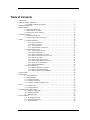
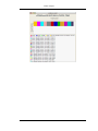
9.3. Color Map
Figure 9.3. Color Map
30
Preferences
The color map shows specifically assigned colors. These values are used across all trials loaded so that
the user can identify a particular function across multiple trials. In order to map an entire trial's function
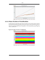
set, Select "Assign Defaults from ->" and select a loaded trial.
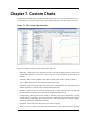
Individual functions can be assigned a particular color by clicking on them in any of the other ParaProf
Windows.
31
PerfExplorer - User's Manual
University of Oregon
PerfExplorer - User's Manual
by University of Oregon
Published (TBA)
Copyright © 2011 University of Oregon Performance Research Lab
Table of Contents
1. Introduction ............................................................................................................ 6
2. Installation and Configuration .................................................................................... 7
2.1. Available configuration options ............................................................... 7
3. Running PerfExplorer ............................................................................................... 8
4. Cluster Analysis ...................................................................................................... 9
4.1. Dimension Reduction ............................................................................. 9
4.2. Max Number of Clusters ......................................................................... 9
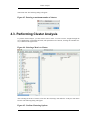
4.3. Performing Cluster Analysis .................................................................. 10
5. Correlation Analysis ............................................................................................... 16
5.1. Dimension Reduction ........................................................................... 16
5.2. Performing Correlation Analysis ............................................................ 16
6. Charts .................................................................................................................. 20
6.1. Setting Parameters ............................................................................... 20
6.1.1. Group of Interest ...................................................................... 20
6.1.2. Metric of Interest ...................................................................... 20
6.1.3. Event of Interest ....................................................................... 20
6.1.4. Total Number of Timesteps ........................................................ 21
6.2. Standard Chart Types ........................................................................... 21
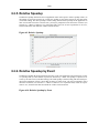
6.2.1. Timesteps Per Second ................................................................ 21
6.2.2. Relative Efficiency .................................................................... 22
6.2.3. Relative Efficiency by Event ....................................................... 22
6.2.4. Relative Efficiency for One Event ................................................ 23
6.2.5. Relative Speedup ...................................................................... 24
6.2.6. Relative Speedup by Event ......................................................... 24
6.2.7. Relative Speedup for One Event .................................................. 25
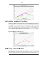
6.2.8. Group % of Total Runtime ......................................................... 25
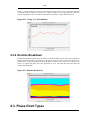
6.2.9. Runtime Breakdown .................................................................. 26
6.3. Phase Chart Types ............................................................................... 26
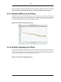
6.3.1. Relative Efficiency per Phase ...................................................... 27
6.3.2. Relative Speedup per Phase ........................................................ 27
6.3.3. Phase Fraction of Total Runtime .................................................. 28
7. Custom Charts ...................................................................................................... 29
8. Visualization ......................................................................................................... 31
8.1. 3D Visualization ................................................................................. 31
8.2. Data Summary .................................................................................... 31
8.3. Creating a Boxchart ............................................................................. 32
8.4. Creating a Histogram ........................................................................... 33
8.5. Creating a Normal Probability Chart ....................................................... 34
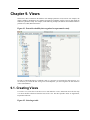
9. Views .................................................................................................................. 36
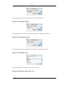
9.1. Creating Views ................................................................................... 36
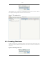
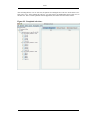
9.2. Creating Subviews ............................................................................... 38
10. Running PerfExplorer Scripts ................................................................................. 40
10.1. Analysis Components ......................................................................... 40
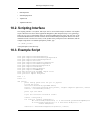
10.2. Scripting Interface ............................................................................. 41
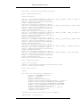
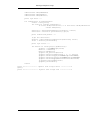
10.3. Example Script .................................................................................. 41
11. Derived Metrics ................................................................................................... 44
11.1. CreatingExpressions ........................................................................... 44
11.2. Selecting Expressions ......................................................................... 44
11.3. Expression Files ................................................................................ 44
iv
List of Figures
4.1. Selecting a dimension reduction method .................................................................... 9
4.2. Entering a minimum threshold for exclusive percentage ................................................ 9
4.3. Entering a maximum number of clusters .................................................................. 10
4.4. Selecting a Metric to Cluster .................................................................................. 10
4.5. Confirm Clustering Options .................................................................................. 10
4.6. Cluster Results .................................................................................................... 11
4.7. Cluster Membership Histogram .............................................................................. 11
4.8. Cluster Membership Scatterplot ............................................................................. 12
4.9. Cluster Virtual Topology ...................................................................................... 13
4.10. Cluster Average Behavior ................................................................................... 14
5.1. Selecting a dimension reduction method .................................................................. 16
5.2. Entering a minimum threshold for exclusive percentage .............................................. 16
5.3. Selecting a Metric to Cluster .................................................................................. 16
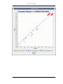
5.4. Correlation Results .............................................................................................. 17
5.5. Correlation Example ............................................................................................ 18
6.1. Setting Group of Interest ....................................................................................... 20
6.2. Setting Metric of Interest ...................................................................................... 20
6.3. Setting Event of Interest ....................................................................................... 20
6.4. Setting Timesteps ................................................................................................ 21
6.5. Timesteps per Second .......................................................................................... 21
6.6. Relative Efficiency .............................................................................................. 22
6.7. Relative Efficiency by Event ................................................................................. 23
6.8. Relative Efficiency one Event ................................................................................ 23
6.9. Relative Speedup ................................................................................................ 24
6.10. Relative Speedup by Event .................................................................................. 24
6.11. Relative Speedup one Event ................................................................................ 25
6.12. Group % of Total Runtime .................................................................................. 26
6.13. Runtime Breakdown .......................................................................................... 26
6.14. Relative Efficiency per Phase ............................................................................... 27
6.15. Relative Speedup per Phase ................................................................................. 27
6.16. Phase Fraction of Total Runtime ........................................................................... 28
7.1. The Custom Charts Interface ................................................................................. 29
8.1. 3D Visualization of multivariate data ...................................................................... 31
8.2. Data Summary Window ....................................................................................... 32
8.3. Boxchart ............................................................................................................ 32
8.4. Histogram .......................................................................................................... 33
8.5. Normal Probability .............................................................................................. 34
9.1. Potential scalability data organized as a parametric study ............................................ 36
9.2. Selecting a table .................................................................................................. 36
9.3. Selecting a column .............................................................................................. 37
9.4. Selecting an operator ............................................................................................ 37
9.5. Selecting a value ................................................................................................. 37
9.6. Entering a name for the view ................................................................................. 37
9.7. The completed view ............................................................................................. 38
9.8. Selecting the base view ........................................................................................ 38
9.9. Completed sub-views ........................................................................................... 39
v
Chapter 1. Introduction
PerfExplorer is a framework for parallel performance data mining and knowledge discovery. The framework architecture enables the development and integration of data mining operations that will be applied
to large-scale parallel performance profiles.
The overall goal of the PerfExplorer project is to create a software to integrate sophisticated data mining
techniques in the analysis of large-scale parallel performance data.
PerfExplorer supports clustering, summarization, association, regression, and correlation. Cluster analysis is the process of organizing data points into logically similar groupings, called clusters. Summarization is the process of describing the similarities within, and dissimilarities between, the discovered
clusters. Association is the process of finding relationships in the data. One such method of association
is regression analysis, the process of finding independent and dependent correlated variables in the data.
In addition, comparative analysis extends these operations to compare results from different experiments, for instance, as part of a parametric study.
In addition to the data mining operations available, the user may optionally choose to perform comparative analysis. The types of charts available include time-steps per second, relative efficiency and speedup
of the entire application, relative efficiency and speedup of one event, relative efficiency and speedup
for all events, relative efficiency and speedup for all phases and runtime breakdown of the application
by event or by phase. In addition, when the events are grouped together, such as in the case of communication routines, yet another chart shows the percentage of total runtime spent in that group of events.
These analyses can be conducted across different combinations of parallel profiles and across phases
within an execution.
6
Chapter 2. Installation and
Configuration
PerfExplorer uses PerfDMF databases so if you have not already you will need to install PerfDMF, see
???. To configure PerfExplorer move to the tools/src/PerfExplorer/ directory in you TAU
distribution. Type:
%>./configure
If you haven't already done so for other TAU tools, add [path to tau]/tau2/apple/bin to
your path.
The following command-line options are available to configure:
2.1. Available configuration options
•
-engine=<analysis engine>
Specifies the data-mining engine to use. The supported options include weka and R.
•
-rroot=<directory>
Specifies the directory where R is installed. Specifically, it should be the directory where the bin,
include, lib, library and share directories are located.
•
-objectport=<available network port>
Specifies the port that the PerfExplorer server should use, when running PerfExplorer in client-server mode. Select an available network port, and make sure that other appropriate network configurations are made (firewalls, etc.). The default port is 9999.
•
-registryport=<available network port>
Specifies the port that the rmiregistry should use, when ruining PerfExplorer in client-server mode.
Select an available network port, and make sure that other appropriate network configurations are
made (firewalls, etc.). The default port is 1099.
•
-server=<server name>
Specifies the fully qualified domain name of the server where PerfExplorer is run, when running
PerfExplorer in client-server mode.
7
Chapter 3. Running PerfExplorer
To run PerfExplorer type:
%>perfexplorer
When PerfExplorer loads you will see on the left window all the experiments that where loaded into
PerfDMF. You can select which performance data you are interested by navigating the tree structure.
PerfExplorer will allow you to run analysis operations on these experiments. Also the cluster analysis
results are visible on the right side of the window. Various types of comparative analysis are available
from the drop down menu selected.
To run an analysis operation, first select the metric of interest form the experiments on the left. Then
perform the operation by selecting it from the Analysis menu. If you would like you can set the
clustering method, dimension reduction, normalization method and the
number of clusters from the same menu.
The options under the Charts menu provide analysis over one or more applications, experiments, views
or trials. To view these charts first choose a metric of interest by selecting a trial form the tree on the
left. Then optionally choose the Set Metric of Interest or Set Event of Interest
form the Charts menu (if you don't, and you need to, you will be prompted). Now you can view a
chart by selecting it from the Charts menu.
8
Chapter 4. Cluster Analysis
Cluster analysis is a valuable tool for reducing large parallel profiles down to representative groups for
investigation. Currently, there are two types of clustering analysis implemented in PerfExplorer. Both
hierarchical and k-means analysis are used to group parallel profiles into common clusters, and then the
clusters are summarized. Initially, we used similarity measures computed on a single parallel profile as
input to the clustering algorithms, although other forms of input are possible. Here, the performance data
is organized into multi-dimensional vectors for analysis. Each vector represents one parallel thread (or
process) of execution in the profile. Each dimension in the vector represents an event that was profiled
in the application. Events can be any sub-region of code, including libraries, functions, loops, basic
blocks or even individual lines of code. In simple clustering examples, each vector represents only one
metric of measurement. For our purposes, some dissimilarity value, such as Euclidean or Manhattan distance, is computed on the vectors. As discussed later, we have tested hierarchical and $k$-means cluster
analysis in PerfExplorer on profiles with over 32K threads of execution with few difficulties.
4.1. Dimension Reduction
Often, many hundreds of events are instrumented when profile data is collected. Clustering works best
with dimensions less than 10, so dimension reduction is often necessary to get meaningful results. Currently, there is only one type of dimension reduction available in PerfExplorer. To reduce dimensions,
the user specifies a minimum exclusive percentage for an event to be considered "significant".
To reduce dimensions, select the "Select Dimension Reduction" item under the "Analysis" main menu
bar item. The following dialog will appear:
Figure 4.1. Selecting a dimension reduction method
Select "Over X Percent". The following dialog will appear:
Figure 4.2. Entering a minimum threshold for exclusive percentage
Enter a value, for example "1".
4.2. Max Number of Clusters
By default, PerfExplorer will attempt k-means clustering with values of k from 2 to 10. To change the
maximum number of clusters, select the "Set Maximum Number of Clusters" item under the "Analysis"
9
Cluster Analysis
main menu item. The following dialog will appear:
Figure 4.3. Entering a maximum number of clusters
4.3. Performing Cluster Analysis
To perform cluster analysis, you first need to select a metric. To select a metric, navigate through the
tree of applications, experiments and trials, and expand the trial of interest, showing the available metrics, as shown in the figure below:
Figure 4.4. Selecting a Metric to Cluster
After selecting the metric of interest, select the "Do Clustering" item under the "Analysis" main menu
bar item. The following dialog will appear:
Figure 4.5. Confirm Clustering Options
10
Cluster Analysis
After confirming the clustering, the clustering will begin. When the clustering results are available, you
can view them in the "Cluster Results" tab.
Figure 4.6. Cluster Results
There are a number of images in the "Cluster Results" window. From left to right, the windows indicate
the cluster membership histogram, a PCA scatterplot showing the cluster memberships, a virtual topology of the parallel machine, the minimum values for each event in each cluster, the average values for
each event in each cluster, and the maximum values for each event in each cluster. Clicking on a thumbnail image in the main window will bring up the images, as shown below:
Figure 4.7. Cluster Membership Histogram
11
Cluster Analysis
Figure 4.8. Cluster Membership Scatterplot
12
Cluster Analysis
Figure 4.9. Cluster Virtual Topology
13
Cluster Analysis
Figure 4.10. Cluster Average Behavior
14
Cluster Analysis
15
Chapter 5. Correlation Analysis
Correlation analysis in PerfExplorer is used to explore relationships between events in a profile. Each
event is pairwise plotted with the other events, and a correlation coefficient is calcuated for the relationship. When the events are highly positively correlated (coefficient of close to 1.0) or highly negatively
correlated (coefficient close to -1.0), then the relationships will show up as linear groupings in the results. Clusters may also be apparent.
5.1. Dimension Reduction
Often, many hundreds of events are instrumented when profile data is collected. Clustering works best
with dimensions less than 10, so dimension reduction is often necessary to get meaningful results. Currently, there is only one type of dimension reduction available in PerfExplorer. To reduce dimensions,
the user specifies a minimum exclusive percentage for an event to be considered "significant".
To reduce dimensions, select the "Select Dimension Reduction" item under the "Analysis" main menu
bar item. The following dialog will appear:
Figure 5.1. Selecting a dimension reduction method
Select "Over X Percent". The following dialog will appear:
Figure 5.2. Entering a minimum threshold for exclusive percentage
Enter a value, for example "1".
5.2. Performing Correlation Analysis
To perform correlation analysis, you first need to select a metric. To select a metric, navigate through
the tree of applications, experiments and trials, and expand the trial of interest, showing the available
metrics, as shown in the figure below:
Figure 5.3. Selecting a Metric to Cluster
16
Correlation Analysis
After selecting the metric of interest, select the "Do Correlation Analysis" item under the "Analysis"
main menu bar item. A confirmation dialog will appear, and you can either confirm the correlation request or cancel it. After confirming the correlation, the analysis will begin. When the analysis results are
available, you can view them in the "Correlation Results" tab.
Figure 5.4. Correlation Results
17
Correlation Analysis
There are a number of images in the "Correlation Results" window. Each thumbnail represents a pairwise correlation plot of two events. Clicking on a thumbnail image in the main window will bring up the
images, as shown below:
Figure 5.5. Correlation Example
18
Correlation Analysis
19
Chapter 6. Charts
6.1. Setting Parameters
There are a few parameters which need to be set when doing comparisons between trials in the database.
If any necessary setting is not configured before requesting a chart, you will be prompted to set the
value. The following settings may be necessary for the various charts available:
6.1.1. Group of Interest
TAU events are often associated with common groups, such as "MPI", "TRANSPOSE", etc. This value
is used for showing what fraction of runtime that this group of events contributed to the total runtime.
Figure 6.1. Setting Group of Interest
6.1.2. Metric of Interest
Profiles may contain many metrics gathered for a single trial. This selects which of the available metrics
the user is interested in.
Figure 6.2. Setting Metric of Interest
6.1.3. Event of Interest
Some charts examine events in isolation. This setting configures which event to examine.
Figure 6.3. Setting Event of Interest
20
Charts
6.1.4. Total Number of Timesteps
One chart, the "Timesteps per second" chart, will calculate the number of timesteps completed per
second. This setting configures that value.
Figure 6.4. Setting Timesteps
6.2. Standard Chart Types
6.2.1. Timesteps Per Second
The Timesteps Per Second chart shows how an application scales as it relates to time-to-solution. If the
timesteps are not already set, you will be prompted to enter the total number of timesteps in the trial (see
Section 6.1.4, “Total Number of Timesteps” ). If there is more than one metric to choose from, you may
be prompted to select the metric of interest (see Section 6.1.2, “Metric of Interest”). To request this
chart, select one or more experiments or one view, and select this chart item under the "Charts" main
menu item.
Figure 6.5. Timesteps per Second
21
Charts
6.2.2. Relative Efficiency
The Relative Efficiency chart shows how an application scales with respect to relative efficiency. That
is, as the number of processors increases by a factor, the time to solution is expected to decrease by the
same factor (with ideal scaling). The fraction between the expected scaling and the actual scaling is the
relative efficiency. If there is more than one metric to choose from, you may be prompted to select the
metric of interest (see Section 6.1.2, “Metric of Interest”). To request this chart, select one experiment or
view, and select this chart item under the "Charts" main menu item.
Figure 6.6. Relative Efficiency
6.2.3. Relative Efficiency by Event
The Relative Efficiency By Event chart shows how each event in an application scales with respect to
relative efficiency. That is, as the number of processors increases by a factor, the time to solution is expected to decrease by the same factor (with ideal scaling). The fraction between the expected scaling and
the actual scaling is the relative efficiency. If there is more than one metric to choose from, you may be
prompted to select the metric of interest (see Section 6.1.2, “Metric of Interest”). To request this chart,
22
Charts
select one or more experiments or one view, and select this chart item under the "Charts" main menu
item.
Figure 6.7. Relative Efficiency by Event
6.2.4. Relative Efficiency for One Event
The Relative Efficiency for One Event chart shows how one event from an application scales with respect to relative efficiency. That is, as the number of processors increases by a factor, the time to solution is expected to decrease by the same factor (with ideal scaling). The fraction between the expected
scaling and the actual scaling is the relative efficiency. If there is more than one event to choose from,
and you have not yet selected an event of interest, you may be prompted to select the event of interest
(see Section 6.1.3, “Event of Interest”). If there is more than one metric to choose from, you may be
prompted to select the metric of interest (see Section 6.1.2, “Metric of Interest”). To request this chart,
select one or more experiments or one view, and select this chart item under the "Charts" main menu
item.
Figure 6.8. Relative Efficiency one Event
23
Charts
6.2.5. Relative Speedup
The Relative Speedup chart shows how an application scales with respect to relative speedup. That is, as
the number of processors increases by a factor, the speedup is expected to increase by the same factor
(with ideal scaling). The ideal speedup is charted, along with the actual speedup for the application. If
there is more than one metric to choose from, you may be prompted to select the metric of interest (see
Section 6.1.2, “Metric of Interest”). To request this chart, select one or more experiments or one view,
and select this chart item under the "Charts" main menu item.
Figure 6.9. Relative Speedup
6.2.6. Relative Speedup by Event
The Relative Speedup By Event chart shows how the events in an application scale with respect to relative speedup. That is, as the number of processors increases by a factor, the speedup is expected to increase by the same factor (with ideal scaling). The ideal speedup is charted, along with the actual speedup for the application. If there is more than one metric to choose from, you may be prompted to select
the metric of interest (see Section 6.1.2, “Metric of Interest”). To request this chart, select one experiment or view, and select this chart item under the "Charts" main menu item.
Figure 6.10. Relative Speedup by Event
24
Charts
6.2.7. Relative Speedup for One Event
The Relative Speedup for One Event chart shows how one event in an application scales with respect to
relative speedup. That is, as the number of processors increases by a factor, the speedup is expected to
increase by the same factor (with ideal scaling). The ideal speedup is charted, along with the actual speedup for the application. If there is more than one event to choose from, and you have not yet selected an
event of interest, you may be prompted to select the event of interest (see Section 6.1.3, “Event of Interest”). If there is more than one metric to choose from, you may be prompted to select the metric of interest (see Section 6.1.2, “Metric of Interest”). To request this chart, select one or more experiments or
one view, and select this chart item under the "Charts" main menu item.
Figure 6.11. Relative Speedup one Event
6.2.8. Group % of Total Runtime
The Group % of Total Runtime chart shows how the fraction of the total runtime for one group of events
changes as the number of processors increases. If there is more than one group to choose from, and you
have not yet selected a group of interest, you may be prompted to select the group of interest (see Sec25
Charts
tion 6.1.1, “Group of Interest”). If there is more than one metric to choose from, you may be prompted
to select the metric of interest (see Section 6.1.2, “Metric of Interest”). To request this chart, select one
or more experiments or one view, and select this chart item under the "Charts" main menu item.
Figure 6.12. Group % of Total Runtime
6.2.9. Runtime Breakdown
The Runtime Breakdown chart shows the fraction of the total runtime for all events in the application,
and how the fraction changes as the number of processors increases. If there is more than one metric to
choose from, you may be prompted to select the metric of interest (see Section 6.1.2, “Metric of Interest”). To request this chart, select one experiment or view, and select this chart item under the
"Charts" main menu item.
Figure 6.13. Runtime Breakdown
6.3. Phase Chart Types
26
Charts
TAU now provides the ability to break down profiles with respect to phases of execution. One such application would be to collect separate statistics for each timestep, or group of timesteps. In order to visualize the variance between the phases of execution, a number of phase-based charts are available.
6.3.1. Relative Efficiency per Phase
The Relative Efficiency Per Phase chart shows the relative efficiency for each phase, as the number of
processors increases. If there is more than one metric to choose from, you may be prompted to select the
metric of interest (see Section 6.1.2, “Metric of Interest”). To request this chart, select one experiment or
view, and select this chart item under the "Charts" main menu item.
Figure 6.14. Relative Efficiency per Phase
6.3.2. Relative Speedup per Phase
The Relative Speedup Per Phase chart shows the relative speedup for each phase, as the number of processors increases. If there is more than one metric to choose from, you may be prompted to select the
metric of interest (see Section 6.1.2, “Metric of Interest”). To request this chart, select one experiment or
view, and select this chart item under the "Charts" main menu item.
Figure 6.15. Relative Speedup per Phase
27
Charts
6.3.3. Phase Fraction of Total Runtime
The Phase Fraction of Total Runtime chart shows the breakdown of the execution by phases, and shows
how that breakdown changes as the number of processors increases. If there is more than one metric to
choose from, you may be prompted to select the metric of interest (see Section 6.1.2, “Metric of Interest”). To request this chart, select one experiment or view, and select this chart item under the
"Charts" main menu item.
Figure 6.16. Phase Fraction of Total Runtime
28
Chapter 7. Custom Charts
In addition to the default charts available in the charts menu, there are is a custom chart interface. To access the interface, select the "Custom Charts" tab on in the results pane of the main window, as shown:
Figure 7.1. The Custom Charts Interface
There are a number of controls for the cusotom charts. They are:
•
Main Only - When selected, only the main event (the event with the highest inclusive value) will be
selected. When deselected, the "Events" control (see below) is activated, and one or all events can be
selected.
•
Call Paths - When selected, callpath events will be available in the "Events" control (see below).
•
Log Y - When selected, the Y axis will be the log of the true value.
•
Scalability - When selected, the chart will be interpreted as a speedup chart. The trial with the fewest
number of threads of execution will be considered the baseline trial.
•
Efficiency - When selected, the chart will be interpreted as a relative efficiency chart. The trial with
the fewest number of threads of execution will be considered the baseline trial.
•
Strong Scaling - When deselected, the speedup or efficiency chart will be interpreted as a strong
scaling study (the workload is the same for all trials). When selected, the button will change to
"Weak Scaling", and the chart will be interpreted as a weak scaling study (the workload is proportional to the total number of threads in each trial).
•
Horizontal - when selected, the chart X and Y axes will be swapped.
•
Show Y-Axis Zero - when selected, the chart will include the value 0. When deselected, the chart
29
Custom Charts
will only show the relevant values for all data points.
•
Chart Title - value to use for the chart title
•
Series Name/Value - the field to be used to group the data points as a series.
•
X Axis Value - the field to use as the X axis value.
•
X Axis Name - the name to put in the chart for the value along the X axis.
•
Y Axis Value - the field to use as the Y axis value
•
Y Axis Name - the name to put in the chart for the value along the X axis.
•
Dimension Reduction - whether or not to use dimension reduction. This is only applicable when
"Main Only" is disabled.
•
Cutoff - when the "Dimension Reduction" is enabled, the cutoff value for selecting "All Events".
•
Metric - The metric of interest for the Y axis.
•
Units - The unit to be selected for the Y axis.
•
Event - The event of interest, or "All Events".
•
XML Field - When the X or Y axis is selected to be an XML field, this is the field of interest.
•
Apply - build the chart.
•
Reset - restore the options back to the default values.
When the chart is generated, it can be saved as a vector image by selecting "File -> Save As Vector Image". The chart can also be saved as a PNG by right clicking on the chart, and selecting "Save As...".
30
Chapter 8. Visualization
Under the "Visualization" main menu item, there are five types of raw data visualization. The five items
are "3D Visualization", "Data Summary", "Create Boxchart", "Create Histogram" and "Create Normal
Probability Chart". For the Boxchart, Histogram and Normal Probability Charts, you can either select
one metric in the trial (which selects all events by default), or expand the metric and select events of interest.
8.1. 3D Visualization
When the "3D Visualization" is requested, PerfExplorer examines the data to try to determine the most
interesting events in the trial. That is, for the selected metric in the selected trial, the database will calculate the weighted relative variance for each event across all threads of execution, in order to find the top
four "significant" events. These events are selected by calculating: stddev(exclusive) / (max(exclusive) min(exclusive)) * exclusive_percentage. After selecting the top four events, they are graphed in an
OpenGL window.
Figure 8.1. 3D Visualization of multivariate data
8.2. Data Summary
In order to see a summary of the performance data in the database, select the "Show Data Summary"
item under the "Visualization" main menu item.
31
Visualization
Figure 8.2. Data Summary Window
8.3. Creating a Boxchart
In order to see a boxchart summary of the performance data in the database, select the "Create Boxchart"
item under the "Visualization" main menu item.
Figure 8.3. Boxchart
32
Visualization
8.4. Creating a Histogram
In order to see a histogram summary of the performance data in the database, select the "Create Histogram" item under the "Visualization" main menu item.
Figure 8.4. Histogram
33
Visualization
8.5. Creating a Normal Probability Chart
In order to see a normal probability summary of the performance data in the database, select the "Create
NormalProbability" item under the "Visualization" main menu item.
Figure 8.5. Normal Probability
34
Visualization
35
Chapter 9. Views
Often times, data is loaded into the database with multiple parametric cross-sections. For example, the
charts available in PerfExplorer are primarily designed for scalability analysis, however data might be
loaded as a parametric study. For example, in the following example, the data has been loaded with three
problem sizes, MIN, HALF and FULL.
Figure 9.1. Potential scalability data organized as a parametric study
In order to examine this data in a scalability study, it is necessary to reorganize the data. However, it is
not necessary to re-load the data. Using views in PerfExplorer, you can re-organize the data based on
values in the database.
9.1. Creating Views
To create a view, select the "Create New View" item under the "Views" main menu item. The first step
is to select the table which will form the basis of the view. The three possible values are Application,
Experiment and Trial:
Figure 9.2. Selecting a table
36
Views
After selecting the table, you need to select the column on which to filter:
Figure 9.3. Selecting a column
After selecting the column, you need to select the operator for comparing to that column:
Figure 9.4. Selecting an operator
After selecting the operator, you need to select the value for comparing to the column:
Figure 9.5. Selecting a value
After selecting the value, you need to select a name for the view:
Figure 9.6. Entering a name for the view
37
Views
After creating the view, you will need to exit PerfExplorer and re-start it to see the view. This is a
known problem with the application, and will be fixed in a future release.
Figure 9.7. The completed view
9.2. Creating Subviews
In order to create sub-views, you first need to select the "Create New Sub-View" item from the "Views"
main menu item. The first dialog box will prompt you to select the view (or sub-view) to base the new
sub-view on:
Figure 9.8. Selecting the base view
38
Views
After selecting the base view or sub-view, the options for creating the new sub-view are the same as creating a new view. After creating the sub-view, you will need to exit PerfExplorer and re-start it to see
the sub-view. This is a known problem with the application, and will be fixed in a future release.
Figure 9.9. Completed sub-views
39
Chapter 10. Running PerfExplorer
Scripts
As of version 2.0, PerfExplorer has officially supported a scripting interface. The scripting interface is
useful for adding automation to PerfExplorer. For example, a user can load a trial, perform data reduction, extract out key phases, derive metrics, and plot the result.
10.1. Analysis Components
There are many operations available, including:
•
BasicStatisticsOperation
•
CopyOperation
•
CorrelateEventsWithMetadata
•
CorrelationOperation
•
DeriveMetricOperation
•
DifferenceMetadataOperation
•
DifferenceOperation
•
DrawBoxChartGraph
•
DrawGraph
•
DrawMMMGraph
•
ExtractCallpathEventOperation
•
ExtractEventOperation
•
ExtractMetricOperation
•
ExtractNonCallpathEventOperation
•
ExtractPhasesOperation
•
ExtractRankOperation
•
KMeansOperation
•
LinearRegressionOperation
•
LogarithmicOperation
•
MergeTrialsOperation
•
MetadataClusterOperation
•
PCAOperation
40
Running PerfExplorer Scripts
•
RatioOperation
•
ScalabilityOperation
•
TopXEvents
•
TopXPercentEvents
10.2. Scripting Interface
The scripting interface is in Python, and scripts can be used to build analysis workflows. The Python
scripts control the Java classes in the application through the Jython interpreter (http://www.jython.org/).
There are two types of components which are useful in building analysis scripts. The first type is the
PerformanceResult interface, and the second is the PerformanceAnalysisComponent interface. For documentation on how to use the Java classes, see the javadoc in the perfexplorer source distribution, and the
example scripts below. To build the perfexplorer javadoc, type
%>./make javadoc
in the perfexplorer source directory.
10.3. Example Script
from
from
from
from
from
from
from
from
from
from
from
from
from
glue import PerformanceResult
glue import PerformanceAnalysisOperation
glue import ExtractEventOperation
glue import Utilities
glue import BasicStatisticsOperation
glue import DeriveMetricOperation
glue import MergeTrialsOperation
glue import TrialResult
glue import AbstractResult
glue import DrawMMMGraph
edu.uoregon.tau.perfdmf import Trial
java.util import HashSet
java.util import ArrayList
True = 1
False = 0
def glue():
print "doing phase test for gtc on jaguar"
# load the trial
Utilities.setSession("perfdmf.demo")
trial1 = Utilities.getTrial("gtc_bench", "Jaguar Compiler Options", "fastss
result1 = TrialResult(trial1)
print "got the data"
# get the iteration inclusive totals
events = ArrayList()
for event in result1.getEvents():
#if event.find("Iteration") >= 0 and result1.getEventGroupName(even
if event.find("Iteration") >= 0 and event.find("=>") < 0:
events.add(event)
extractor = ExtractEventOperation(result1, events)
41
Running PerfExplorer Scripts
extracted = extractor.processData().get(0)
print "extracted phases"
# derive metrics
derivor = DeriveMetricOperation(extracted,
derived = derivor.processData().get(0)
merger = MergeTrialsOperation(extracted)
merger.addInput(derived)
extracted = merger.processData().get(0)
derivor = DeriveMetricOperation(extracted,
derived = derivor.processData().get(0)
merger = MergeTrialsOperation(extracted)
merger.addInput(derived)
extracted = merger.processData().get(0)
derivor = DeriveMetricOperation(extracted,
derived = derivor.processData().get(0)
merger = MergeTrialsOperation(extracted)
merger.addInput(derived)
extracted = merger.processData().get(0)
derivor = DeriveMetricOperation(extracted,
derived = derivor.processData().get(0)
merger = MergeTrialsOperation(extracted)
merger.addInput(derived)
extracted = merger.processData().get(0)
derivor = DeriveMetricOperation(extracted,
derived = derivor.processData().get(0)
merger = MergeTrialsOperation(extracted)
merger.addInput(derived)
extracted = merger.processData().get(0)
derivor = DeriveMetricOperation(extracted,
derived = derivor.processData().get(0)
merger = MergeTrialsOperation(extracted)
merger.addInput(derived)
extracted = merger.processData().get(0)
"PAPI_L1_TCA", "PAPI_L1_TCM", De
"PAPI_L1_TCA-PAPI_L1_TCM", "PAPI
"PAPI_L1_TCM", "PAPI_L2_TCM", De
"PAPI_L1_TCM-PAPI_L2_TCM", "PAPI
"PAPI_FP_INS", "P_WALL_CLOCK_TIM
"PAPI_FP_INS", "PAPI_TOT_INS", D
print "derived metrics..."
# get the Statistics
dostats = BasicStatisticsOperation(extracted, False)
stats = dostats.processData()
print "got stats..."
return
for metric in stats.get(0).getMetrics():
grapher = DrawMMMGraph(stats)
metrics = HashSet()
metrics.add(metric)
grapher.set_metrics(metrics)
grapher.setTitle("GTC Phase Breakdown: " + metric)
grapher.setSeriesType(DrawMMMGraph.TRIALNAME);
grapher.setCategoryType(DrawMMMGraph.EVENTNAME)
grapher.setValueType(AbstractResult.INCLUSIVE)
grapher.setXAxisLabel("Iteration")
grapher.setYAxisLabel("Inclusive " + metric);
# grapher.setLogYAxis(True)
grapher.processData()
# graph the significant events in the iteration
subsetevents = ArrayList()
42
Running PerfExplorer Scripts
subsetevents.add("CHARGEI")
subsetevents.add("PUSHI")
subsetevents.add("SHIFTI")
print "got data..."
for subsetevent in subsetevents:
events = ArrayList()
for event in result1.getEvents():
if event.find("Iteration") >= 0 and event.rfind(subsetevent
events.add(event)
extractor = ExtractEventOperation(result1, events)
extracted = extractor.processData().get(0)
print "extracted phases..."
# get the Statistics
dostats = BasicStatisticsOperation(extracted, False)
stats = dostats.processData()
print "got stats..."
for metric in stats.get(0).getMetrics():
grapher = DrawMMMGraph(stats)
metrics = HashSet()
metrics.add(metric)
grapher.set_metrics(metrics)
grapher.setTitle(subsetevent + ", " + metric)
grapher.setSeriesType(DrawMMMGraph.TRIALNAME);
grapher.setCategoryType(DrawMMMGraph.EVENTNAME)
grapher.setValueType(AbstractResult.INCLUSIVE)
# grapher.setLogYAxis(True)
grapher.processData()
return
print "--------------- JPython test script start ------------"
glue()
print "---------------- JPython test script end -------------"
43
Chapter 11. Derived Metrics
Sometimes metrics in a profile need to be combined to create a derived metric. PerfExplorer allows the
user to create these using the derived metric expression tab.
11.1. CreatingExpressions
The text box at the top of the tab allows the user to enter an expression. Double clicking on a metric in
the "Performance Data" tree will copy that metrics name into the box. If a metric contains any operands,
the whole metric must be surrounded by quotes. If the you would like of the metric to be renamed, then
you should start the expression with the new name and and equals sign.
If this is the only metric you wish to derive, then select the trial, expression or application where the
metric should be derived and then click apply. If you wish to derive many metrics, then click Add to List
and create more expressions.
11.2. Selecting Expressions
If you have added multiple expressions, you can select one or many of them to apply. They will be derived from top to bottom. After you have select some, you can select the trial, experiment or application
to apply the expression to and then click apply.
11.3. Expression Files
You can also derive metrics using an expression file. An expression file has a single expression per line.
To parse the file, select the trial, experiment or application to apply the expressions to; then select File >
Parse Expression File and chose the file.
44