Download Get Started with InteGriTy

InteGriTy
User’s guide
Version 1.0.- Feb. 03
1
1. About InteGriTy
InteGriTy is a Fortran90 free software package that allows to perform topological analysis following the AIM (Atoms
In Molecules [1]) approach on electron densities given on three-dimensional grids. It consists of 2 programs. The first one
cpgrity.f90” performs critical points (CPs) search and computes their properties. It is also used to search for bond paths
from the (3,-1) CPs. The second program, “integrity.f90” determines the boundaries of atomic basins and computes
integrated atomic properties (surface, volume, charge and multipoles).. The programs can handle both periodic (translation
symmetry) or non periodic systems.
CP search: to locate CPs, gradient path is followed with a classic Newton method starting from each grid point. If a CP
is not found within a limited travelled distance the next grid point is considered, etc.
Atomic Basins: atomic basins are determined from their single surface intersection with rays originating from the
attractors. A “coarse” estimation of the atomic surface is first performed, sufficient for graphics purpose and to yield first
estimates during the “fine” search which occurs while performing integration. Integrated quantities are total and valence
electron densities, Laplacian, dipolar and quadrupolar moments, volume and surface. Romberg integration method is used
to automatically adapt the number of integration steps to a desired convergence level for each basin. Two density data files
are given as input for integration. The first one gives the total density and the second one gives partial density, as for
example sole valence electron density. This allows better estimation of integrated quantities.
More details can be found in C. Katan, P. Rabiller, C. Lecomte, M. Guezo, V. Oison and M. Souhassou., J. Appl. Cryst.
(2003) 36, 65-73.
! Please cite the above reference when publishing results coming from InteGriTy.
[1] R.F.W. Bader, Atoms in Molecules: A Quantum Theory, Int. Series of Monographs on Chemistry 22 (Oxford, 1990)
2. Few remarks
This User’s Guide is the second draft of all we have ever written yet ! Please, be comprehensive … Any suggestions on
how to improve the clarity of this Guide, the performance of the codes are mostly welcome. Graphical routines, using
Matlab® are now available and soon free OpenDx solution too.
2
3. Before starting
In order to start a CP search the “cpgrity.f90” has to be compiled . This program uses 3 input files. To compute atomic
properties you need to compile “integrity.f90”. This program uses 5 input files. Both programs produce a variable number
of output files according to the possible tasks that have been performed. All output files are ASCII ones.
4. Input files
Input files are of two different types:
 TYPE 1 : density given on a grid
 TYPE 2 : atomic positions, file names, file paths, file extensions and parameters which define how the programs
should run. Most of these information are specified by extensive use of keywords.
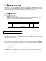
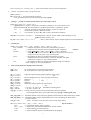
The following table gives the filenames used in this User’s Guide . In this table, “F” indicates that filename or extension is
fixed whereas “C” indicates that it can be specified by the user.
TYPE
1
1
2
2
2
cpgrity.f90
sample-tot.data
data.in
cpgrity.in
integrity.f90
sample-tot.data
sample-val.data
data.in
integrity.in
ATOMPAR.inp
file name
C
C
C
F
F
file extension
C
C
F
F
F
4.1 Density data files
Default file extensions are “-tot.data” for the total density and “-val.data” for the sole valence density. Other extensions
can be specified either in cpgrity.in or in integrity.in. Throughout this User’s Guide the generic file name “sample” will be
used. In all cases, the generic file name must be specified on the first line of the file data.in. The program integrity.f90
needs both sample-tot.data and sample-val.data input files (the same file can be used for both total and valence) whereas
cpgrity.f90 needs only sample-tot.data.
Density data files are binary files. All input data must be given in atomic units which means that the electron density is
given in e-/au3 . Double precision works best; if not, a precision of 10-6 e-/au3 is recommended.
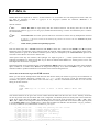
The grid metrics is given first: number of grid points in the three directions (labelled hereafter 1,2,3), grid origin
respective to the absolute cartesian system origin to which the atomic positions are referred to and the three elementary
vectors defining the length and directions of the grid mesh. These quantities are read according to the following Fortran90
statements:
read(unit)np1,np2,np3
read(unit)origin
read(unit)del1
read(unit)del2
read(unit)del3
Then the density “rho(i,j,k)” at all the grid points is read according to the following loops (be aware of the k,j,i, order !!).
&
&
&
&
read(unit) &
(((rho(i,j,k) &
,k=1,np3) &
,j=1,np2) &
,i=1,np1)
3
4.2 data.in
Default name for this input file is “data.in”. Its file extension “.in” is fixed but users can change the file name “data” into
any other by specifying it either in cpgrity.in or in integrity.in (without the extension: data=data ! or
data= another_filename!).
This file contains:
1st line:
Generic file name of input density data files without extension. The density files will be read with
extensions given either in cpgrity.in or in integrity.in, default extensions beeing “-tot.data” for total density and “-val.data”
for valence density.
2nd line:
factor
conversion factor for atomic positions which are converted to atomic units by multiplication with this
3rd ,… :
atomic names, positions and optional properties
(if scale unit = -1, cell units are assumed, the box defined by the grid must be the cell unit in that case. WARNING: may not be
implemented yet !!!!)
Each line must begin with !ATOM and finish with !END. It must also contain at least NAME= and R= keywords
followed by their corresponding values. Other keywords are optional. Atoms labels must be given between single quotes.
Atomic positions are given in an absolute Cartesian system. They are multiplied by the conversion factor given in the
second line of this file for conversion to atomic units.
Atoms species with only one character, like hydrogen “H” might be given a “_” before specific label. For example
hydrogen atom labeled “1a” must be given like “H_1a” where as chlorine atoms labeled “33” will be given as “Cl33”. The
total length must be less than or equal to 6
Optional keywords can be specified for the program integrity. RMIN= allows one to change the radius of the minimum
sphere included in an atomic basin, MULT= to change the multiplicity of an atom and MOL= to give each atom a
molecule number to perform summation over molecules at the end of the integration run.
The last line of the file must begin with !EOB statement.
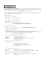
Below you will find an example which tells that total and valence density file names are given by the concatenation of
“sample” and respective extensions “-tot.data” and “-val.data”. A scale unit of one is used, this means that atomic
coordinates are given in cartesian atomic units. The atom “H_1” will have a minimum basin radius of 0.2 au. and will
belong to the first molecule.
sample
1.00000
!ATOM NAME='H_1' R= -1.77112
!EOB
-4.33114
-6.53800
RMIN=0.2 MOL=1 !END
-------------------------------------------------------------------------------------------------------------------------------------------------Non nuclear attractors can be given with “atoms’ names that must differ from the ones reserved for “dummy” atoms that
can also be present in the list and which will not be “integrated”. The dummy atoms are mainly used to focre molecules’
origin. Their generic label will be “DO”. For example, “DO3” will give the origin of molecule “3”. “DU”, “CP”, “CG”,
“RG”, “SL”, ”SH” are reserved generic names for dummy atoms or critical points that can be used to define precise planes
in case working mode is set to “work=plane!). These reserved names are defined in the subroutine “integrity_initialize”,
in an array of character (*2) and dimension 9 named “at_check_list”:
at_check_list(1)='DU'
at_check_list(2)='DO'
at_check_list(3)='CP'
at_check_list(4)='SH'
at_check_list(5)='SL'
at_check_list(6)='CG'
at_check_list(7)='RG'
at_check_list(8)='__'
at_check_list(9)='__'
!!
!!
!!
!!
!!
!!
!!
!!
!!
dummy atom, generally unit cell vortices
dipole orogine (molecular)
generic critical point
saddle point (high density)
saddle point (low density)
cage CP
ring CP
not yet defined (user choice)
not yet defined (user choice)
-------------------------------------------------------------------------------------------------------------------------------------------------4
4.3 cpgrity.in
This file is needed by the program cpgrity.f90. It has to be located at the same place where the program will run. It
contains the pathway for all other input files. cpgrity.in also gives the user the possibility to change almost all the
parameters used in the program. New values are given with the help of keywords with the syntax:
keyword = value !
with one keyword per line and omitted lines either beginning with “!!” (commented line) or postponed after a “EOB!”
statement. An example is given at the end of this section.
The parameters are:

file extension for density data filename
ext = extension !

pathway and (data & atoms) specifications' file
path = pathway !
file = atoms_file !

default value is –tot.data
the program aborts if missing
this correspond to the data.in file described in this manual
atoms_file.in file must exist in the directory specified by path.
Include attractors in the search
cp_type = may contains attractor or not !

grid type : periodic or isolated system
if attractor then search also for CP = maxima
(¡¡¡ needs very fine grid mesh, ~ 0.05 ua !!!)
grid = may contain “iso” or not !
if grid argument is empty or not specified, translation symmetry is used (periodic boundaries condition). For N
points in one direction and mesh dx, the cell parameter is N x dx and point N+1 is equivalent to point 1.
“iso”
=>
“isolated” grid with no translation symmetry. If there is N points in.
one direction, points 4 to N-4 will be used.

Parameters affecting the following of the gradient path
invfric = 0.2 !
dgradmin= 1e-11!
rioff= 1.5 !

friction coefficient applied to H-1·rho(r)
ending threshold for CP location
maximum distance travelled from a grid point following the gradient
then go to the next grid point
Parameters affecting the interpolation (may be obsolete !!!)
mrho = may be 1,0 or -1!
if 1, then search from rho(r) (normal way)
if 0, then search from log(rho(r) + min(rho))
if –1, then search from –rho(r), maxima  minima, etc.
recommended value: 1

Parameters affecting arrays dimension
ncmax = 5000!
maxat = 52!

maximum number of found CPs that can be handled before sorting
maximum number of atoms generated by translations (periodic images)
obsolete!
Parameters affecting eigenvalues determination (curvatures from hessian matrix)
epsoff = 1e-10!
Threshold for the sum of off diagonal elements above which diagonalisation
must be carried out
5

Parameters affecting sorting of CP
densmaxcp = 5e-1!
densoffcp = 5e-3!
lam_0 = 1e-6!

threshold density (e/au3) for saddle points to be considered “high” or “low”
density
threshold density (e/au3) below which CPs are not considered
threshold value for curvature “lambda” below which considered equal to zero
(affect the rank and signature)
Parameters affecting bond path location
densmaxcp =
max_bond_length=3.8!
bond_path_increment=1.d-04!
bond_path_xdo= 5.d+01!
bond_path_dmax=8.d0!
bond_path_nmax=80000!
bond_path_d2at=0.05!
bond_path_dwrite=0.1
maximum "straight" bond length for output
increment for Runge Kutta bond path search
"xdo" x "increment" = distance from (3,-1) CP for starting bond path search along 3
maximum run out distance for bond path search termination
maximum number of bond path search steps before termination
distance from running point to atom for bond path search termination
increment for bond path output writing
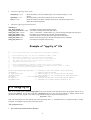
Example of "cpgrity.in" file
!!
!!
!!
!!
!!
!!
!!
!!
!!
!!
!!
!!
!!
!!
!
* List of key-words that can be supplied to the program "cpgrity"
* Lines beginning with "!!" are not considered (comment lines)
* The values corresponding to the key-words are delimited
after the key word on the left by "=" and on the right by '!'
The latter may be omitted, in that case its location is
replaced by the end of the line
* Lines corresponding to numerical values that are not to be modified
must be deleted, commented or put after a line beginning with 'END!' or 'EOB!',
a null value would be attributed otherwise !
path=c:\philippe\topologie\adp\! !! pathway to data and results files directory
file=data!
!! generic atom file-name
cp_type=attractor!
!! tells wether or not attractors are searched
grid=periodic!
!! tells wether or not periodicty is used extension =tot.data!
!! data filename extension
invfric=0.1!
!! friction coefficient used with newton method
dgradmin=1e-8!
!! threshold for ending newton method at CP
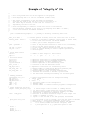
4.4 integrity.in
This file is needed by the program integrity.f90. It has to be located at the same place where the program will be run. It
contains the pathway for all other input files. integrity.in also gives the user the possibility to change almost all the
parameters used in the program. New values are given with the help of keywords with the syntax:
keyword = value !
with one keyword per line and omitted lines either beginning with “!!” (commented line) or postponed after a “EOB!”
statement. An example is given at the end of this section..
The parameters are:

file extension for total and valence densities
6
ext = extension_tot | extension_val ! “|” must be put between the two extension arguments

pathway and (data & atoms) specifications' file
path = pathway !
file = atoms_file ! the program aborts if missing
atoms_file.in file must exist in the directory specified by path.

grid type : periodic or isolated system and van der waals surface check
grid = may contain “iso” and/or “vdv” !
if grid argument is empty or not specified, translation symmetry is used. For N points in one
direction and mesh dx, the cell parameter is N x dx and point N+1 is equivalent to point 1.
“iso”
=>
“isolated” grid with no translation symmetry. If there is N points in.
one direction, points 2 to N-2 will be used.
“vdv” =>
a cut-off value, given by rho_vdv, is used to limit basin boundaries.
rho_vdv = any positive real value !
threshold density value for van der Waals surface limitation in case
grid= statement contains “vdv”
tot_use = may contain “tot” or “val” !
total or valence density used to compute laplacian sum and multipoles

possible jobs
work = may contain “auto”, ”grid”, “manual”, “plane”, “basin” or “line” !
“auto” (default)
=> complete integration over all atoms with Romberg procedure
“grid”
=> integration over all atoms with “fixed spherical grid” integration
obsolete!
“manual”
=> single radial, phi (= radial + phi) or theta (= radial + phi+theta)
integration (for each atom the user is asked for the kind of desired partial
integration and at which phi or phi and theta[rad])
“plane”
=> interpolation of density its gradient and laplacian in a plane
and determination of atomic basins contours in that plane. The plane
is defined in “integrity.in” file or from keyboard
“line”
=> interpolation of density its gradient and laplacian along a line defined
in the “integrity.in” file or from keyboard

basin search parameters (default values indicated)
nth = 30 !
nphi = 60 !
dr_c = 5.d-02 !
dr_f = 5.d-04 !
ea_c = 0.25d0 !
ed_c = 0.50d0 !
ea_f = 0.03d0 !
ed_f = 0.03d0 !
dtol_c = 5.d-02 !
dtol_f = 5.d-04 !
fa_c = 5.d0 !
fa_f = 200.d0 !
exp_dg = 15.d-01 !
max_step_fwd = 3 !
min_step_dwd = 5 !
coef_d = 0.98 !
Nb. of theta points for coarse basin limits search
Nb. of phi points for coarse basin limits search
minimum increment along gradient path for coarse search
"
"
"
"
" " fine "
forward magnification for coarse boundary bracketing
backward
"
"
"
"
"
forward
"
" fine
"
"
backward
"
" "
"
"
dichotomy ending tolerance for coarse search
"
"
"
" fine "
=> dr_max = fa_coarse x dr maximum accelerating factor
=> dr_max = fa_fine x dr
cosine(r,grad_rho) exponent for accelerating step following gradient.
step along gradient path is given by dr x fa x exp[-exp_dg x cosine(r,grad_rho)]
maximum number of steps following gradient outward attractor before declaring it outside
minimum number of steps downward attractor in case of reaching box limit with no
periodic condition
dmin = coef_dmin x rlim_min after coarse search (safety factor)
out = may contain “basi”, “long”, “romb”, “mult” !
may be obsolete !
“basi”
=> output atomic basins’ file for graphics
“basi”+“long” => output basin with additional information on basin surface
“romb”
=> output romberg procedure evolution
“mult”
=> output multipoles (dipole and quadrupole) file for graphics
7

romberg procedure or “regular” theta, phi integration
convergence_test = val_vol ! selects which quantities are used as convergence criteria for
romberg procedure. May also contain “tot”, “lap”
nmax = 20 ! maximum possible number of iterations (remains from Fortran77 original routine)
jmax = 16 ! effective maximum number of iterations jmax < nmax (Fortran77)
kmax = 5 ! polynomial interpolation order for romberg method
kmin = 6 !
minimum iteration number before result of interpolation is effectively taken into account
eps_r = 1.0e-6 !
tolerance for ending “radial” level of integration (relative variation)
eps_phi = 1.0e-4 !
tolerance for ending “phi” level of integration
eps_theta = 1.0e-4 ! tolerance for ending “theta” level of integration
stat = may contain “romb” ! => computes integration steps stactistics (number of radial,
phi, theta and total number of loops)
obsolete !
ntg = 60 !
number of theta points, phi points npg = max (4, int( 2*sin(theta)*ntg))
for fixed spherical grid integration (work = grid !)
nrg = 120 ! number of radial points drg = rlim(theta,phi) / nrg (work = grid !)

obsolete !
obsolete !
plane definition, (require work=plane!)
plane_def = this file or interactive!
tells how the plane is defined
!! "this_file" --> plane input parameters in this file
!! "interactive" --> inputs by user from display and keyboard
!! if no "atom1","atom2" and "atom3" are given, then
!! a plane parallel to (i,j) grid basal plane is used
atom1 =atom label!
Gives the name of atom or CP or pseudo atom defining plane origin
atom2 =atom label!
Gives the name of atom or CP or pseudo atom defining plane Ox axis
atom3 =atom label!
Gives the name of atom or CP or pseudo atom defining plane inclination
middle_23 =yes or nol! Tells if Ox axis is switched or not to middle of atoms 2&3
perppl = parallel or xz or yzl!
Tells perpendicular plane is used (xz or yz instead of xy) or not
centring =molecular or whateverl! If “molecular” then center plane on center of molecule given by atom 1
unless the plane is centered on atom1
incx =value in a.u.!
Gives the plane increment in Ox direction
incy =value in a.u.!
Gives the plane increment in Oy direction
nx =value in a.u.!
Gives the number of plane increment in Ox direction
ny =value in a.u.!
Gives the number of plane increment in Oy direction
nz= value in a.u!
if (dzo .ne. 0 .and. nz>1) "nz" plane processed starting from z_offset=0
if (dzo .ne. 0 .and. nz==1) one plane processed at z_offset=dzo
dxo =value in a.u.!
Gives the plane offset in Ox direction (unless centring=molecular!)
dyo =value in a.u.!
Gives the plane offset in Oy direction (unless centring=molecular!)
dzo =value in a.u.!
Gives the plane offset in Oz direction (always active if non zero)
nal =integer.!
Gives the number of angular steps used to search the basins’ contour in the plane
tol2plane =integer.!
Distance of surface basins points issued from coarse search to the studied plane
this criterion is used to know if a basin crosses the plane. If this number of points
is sufficient (>5) the center of mass of this points projected onto the plane is used
as the origin of the ray intercepting the basin contour exactly in the plane during
the fine search of basin contour.
8
Example of "integrity.in" file
!!
!!
!!
!!
!!
!!
!!
!!
!!
!!
!!
!!
!!
!!
!
!
!
* List of key-words that can can be supplied to the program
* Lines begining with "!!" are not considered (coment lines)
* The values corresponding to the key-words are delimited
after the key word on the left by "=" and on the right by '!'
The latter may be omitted, in that case its location is
replaced by the end of the line
* Lines corresponding to numerical values that are not to be modified
must be deleted, comented or put after a line begining with 'END!' or 'EOB!',
a null value would be attributed otherwise !
path =c:\subdirectory\sample\!
data_file =data !
working_mode = manual !
grid = periodic !
rho_vdv = 1.d-04!
tot_use = tot !
!
! coarse basin search
nth=36 !
nph=72 !
!
! fine basin search
ea_f=0.03 !
ed_f=0.03 !
dr_f=1e-4 !
fa_fine=2500.d0 !
dtol_f=1e-4 !
!
exp_dg=5.d-01 !
max_step_fwd = 4!
min_step_dwd = 5!
!! pathway to directory containing data files
!! contains generic filename, scale unit factor and list of atoms
!! selection of automatic (romberg), regular grid or manual mode;
!! in the later case the user can choose between
!! radial, phi or theta integration level
!!
!!
!!
!!
!!
tells if the periodic condition is used or not ("isolated"),
and if "van der waals" surface is used
in that case a density threshold value must be supplied
total or valence density is used to compute laplacian sum
and multipoles
!! number of theta steps for
!!
"
"
phi
"
"
!!
!!
!!
!!
!!
basin search
"
"
expansion coefficient for forward bracketting
expansion coefficient for downward bracketting
minimum stepsize following gradient path
maximum amplitude of the accelerating factor
tolerance to end the dichotomic search
!! exponential coefficient for accelerating factor
!! maximum number of steps before declaring gradient path
!! leading outside the considered basin
!! minimum number of steps following gradient path
!! downward the attractor to declare a point inside
!! the basin when reaching box boundary for isolated system
!
! romberg procedure
convergence =val_vol !
!! select the properties used for integration ending
eps_r=1e-5 !
!! radial level
eps_phi=5e-3 !
!! phi
"
eps_theta=5e-3 !
!! theta
"
kmax = 5 !
!! polynomial order for the interpolation
jmax = 16 !
!! maximum order
kmin = 6 !
!! minimum number of iteration before polynomial interpolation
!
! output quantities and files
output= basin_multipole_long!
!! writes output files for basin or romberg details
!! for basin output, "long" means that total and valence
!! densities and gradients on the basin boundary are added
!! "multipole" -> dipole and quadrupole file
stat= romb_grad !
!! selection of different statistics output on main output file
!! "romb" --> numbers of loops ...
!! "grad" --> min and max of rho and grad(rho) encountered
!
plane_def= this_file!
!! if running mode is set to "plane", tells how the plane is defined
!! "this_file" --> plane input parameters in this file
!! "interactive" --> inputs by user from display and keyboard
!!
if no "atom1","atom2" and "atom3" are given, then
!!
a plane parallel to (i,j) grid basal plane is used
!
atom1= !
atom2= !
atom3= !
middle_23= no !
9
perp_plane= no !
centering= none!
incx=0.1!
incy=0.1!
nx=80!
ny=80!
dxo=0.d0!
dyo=0.d0!
dzo=3.14696d0!
nz=3!
!! if (dzo .ne. 0 .and. nz>1) "nz" plane processed starting from z_offset=0
!! if (dzo .ne. 0 .and. nz==1) one plane processed at z_offset=dzo
nal=720!
tol2plane=1!
npcp=5!
!
EOB!
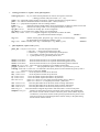
4.5 ATOMPAR.inp
This file is needed by the program integrity.f90. It has to be located at the same place where the program will run. It
contains the names of atomic species, the number of “total” and “valence” electrons of each atom and default values for
the “starting radial value” (in atomic units) used for basin search and the “minimum atomic basin radius” defining the
minimum core of an atomic basin. When a gradient path comes into this minimum core the starting point is considered to
belong to this atomic basin. The number of declared species must be given on first line.
Example:
2
H_
Cl
1
17
1
7
1.20000
3.70000
0.70000
1.80000
Here, 2 species are known and chlorine atom has 17 total electrons, 7 valence electrons. The default minimum basin radius
fo “Cl” atoms is set to 1.8 au. and the initial starting basin search radius is set to 3.7 au. Any pseudo atom can be defined if
necessary. Atom name with a single character must be given with ‘_’ on the right side, like ‘H_’ in this small example.
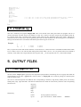
5. OUTPUT FILES
5.1 From cpgrity.f90
The file named “sample.report” reports the most important input parameters used during the run of cpgrity.f90. When the
program aborts, an error file “ cpgrity.error” will be created. A “sample.path” file is used for ploting CP's and bond path
with the matlab routine..
The CPs are sorted and printed into different files corresponding to attractors, high density saddle points, low density
saddle points, rings, cages and others. The later file contains the CPs which do not fit into any other file. The corresponding
extensions are:
-attractors
-saddle-hd
-saddle-ld
-ring
-cage
-other
followed by:
.results
list CP properties extensively
-cp.list
give a list of CPs for “matlab routines”
obsolete!
10
For example “sample-saddle-ld.result” will give, in an extensive presentation of the (3,-1) saddle points properties derived
from an input density given in the file “sample-tot.data”. These CPs have a density lower than the value specified by the
keyword “densmaxcp” of the input file cpgrity.in.
In the source code, outputs to files formerly used with Data Explorer may be still present and are commented. They correspond to extensions “-per.dx”
and “-box.dx” (logical units 15 and 16). An ascii file “c2f.mtx” file is created that stores the transformation matrix from cartesian to unit cell
coordinates.
obsolete!
5.1 From integrity.f90
The file named “sample.integration” reports all parameters used during the run of integrity.f90 and all results. When the
program aborts, an error file “ integrity.error” is created.
All other ASCII output files are devoted for graphics with Matlab® but can be used to prepare input files for other
graphical tools. The Matlab® file "new_plot.m" in conjunction with "new_plot.fig" and other related files allows you to
plot various things (molecules, basins, CP's, bond parths) but you need the commercial Matlab® licence. This graphics
output program uses the extension of the output files to automatically select the adapted graphics. The possible extensions
and graphics are:
“sample.basin” =>
“sample.plane” =>
“sample.line”
=>
“sample.romberg”
draws 3D basins and molecular skeletons in the grid box
draws 2D basins intersection with a plane + molecular skeleton
+ density contours and gradient arrows in the plane
not available now !
gives density, gradient modulus and laplacian along a line
not available now !
=>
records romberg procedure progress.
obsolete !
And for a given atom, for example H_1 (no graphical routines given for that, take your favourite one):
“H_1.radial”
=>
plot of Romberg procedure evolution for radial integration
“H_1.phi”
=>
same for radial + phi integration
“H_1.theta”
=>
same for radial + phi + theta integration
Example:
To plot 3D atomic basins obtained from files located in the directory \user\topology\ with the generic density filename
“sample” first execute Matlab launching. Then select directory where is located new_plot.m. Then enter in the matlab
command window the command : new_plot. Then play with the different "menus". There are still bugs in the graphics
routine, just report them so we can find remedies. For the isodensity plots, the input format for the density is the one used
with another software "XCrysDen". You have to convert the density file to this format. Ther will be soon graphics routines
running under OpenDx which will be more homogeneous and user friendly.
5.1 To prepare”data.in” file
You may use “prepat.m” matlab routine to prepare your “data.in” file. Youcan provide a “prepat.in” wich contains a
title, cell parameters and angles, atoms name, position (in cell unit) and multiplicity and maybe a space group filename. If it
does not exist, these information are asked from prompt and the file will be created. In case only assymetric unit is given,
the whole positions of a space group can be obtained if you have prepared a “space group” file containing all the symmetry
operations and generators, in the form of matrices and row vectors, see for example the “sg167.in” file. Either wise stated,
the symmetry operations can be given one by one. A file with the good format for IntGriTy is created with the entered
11
positions, a file that you can edit The positions generated after symmetry operation are visualized on a plot and displayed
on screen. If you are happy with them just play with “copy and paste” to add them on your “data.in” file. If you use the
option that creates all positions inside the box (0 <= x,y,z < 1) and allows for extra ones outside the box. The one lying
outside the box will be given a zero multiplicity, such that they will count nothing when summing up at the end of integrity.
That’s all for present, now we hope you’ll enjoy it.
Please, feel free to contact us if any problem.
12