Download User Guide

Gaussian Mixture Model Uncertainty Learning (GMMUL)
Version 1.0
User Guide
Alexey Ozerov 1 , Mathieu Lagrange
2
and Emmanuel Vincent
1
1
INRIA, Centre de Rennes - Bretagne Atlantique
Campus de Beaulieu, 35042 Rennes cedex, France
2
IRCAM, STMS, UPMC, CNRS - UMR 9912
1 place Igor Stravinsky, 75004 Paris
{alexey.ozerov, emmanuel.vincent}@inria.fr, [email protected]
January 10, 2012
1
Introduction
This user guide describes a method that can be considered for learning Gaussian Mixture Models
(GMMs) while acknowledging the fact that the data can be uncertain. The level of uncertainty
can be known or estimated. In order to fully grasp the theoretical aspects of the method as well as
the practical facts that motivated the proposal of this method, the reader is strongly encouraged
to read the following papers [1] [2] that will continuously be referred to in the remaining of this
document.
This guide is organized as follows. Section 2 describes the two core functions that allows the
user to learn GMMs from uncertain data. Those functions are then presented within two evaluation
frameworks respectively considered in [1] and [2]. Section 3 describes the first one that focus on
synthetic data, i.e. observed data and uncertainty is generated from sampling of GMMs. Section
4 describes the second one, that considered noisy speech data where the uncertainty is known as
a prior or estimated.
2
2.1
Processing Functions
GMM EM uncertainty learning
The core function is GMM EM uncertainty learning that implements a new Expectation-Maximization
(EM) algorithm for learning GMMs from uncertain data. It can be considered for the purpose of
training GMMs and decoding GMMs, both with handling of uncertainty.
1
f u n c t i o n [ uXe , cXe , wXe , l o g _ l i k e _ N , l ] = . . .
G M M _ E M _ u n c e r t a i n t y _ l e a r n i n g ( y , cE , uX , cX , wX , n b I t e r a t i o n s ,
%
%
%
%
%
%
%
%
%
%
%
%
%
%
%
%
%
%
%
%
%
%
%
%
%
%
%
%
%
%
%
%
%
%
%
%
%
%
%
%
%
%
[ uXe , cXe , wXe , l o g l i k e N , l ] = . . .
GMM EM uncertainty learning ( y , cE , uX , cX , wX,
nbIterations ,
print_log_flag )
print log flag ) ;
E x p e c t a t i o n −m a x i m i z a t i o n (EM) a l g o r i t h m f o r t r a i n i n g G a u s s i a n m i x t u r e
models (GMMs) from n o i s y o b s e r v a t i o n s w i t h G a u s s i a n u n c e r t a i n t y
input
−−−−−
y
cE
uX
cX
wX
nbIterations
print log flag
where
: o b s e r v a t i o n s (N v e c t o r s o f l e n g t h M) , (M x N) m a t r i x
: ( opt ) Gaussian u n c e r t a i n t y , f u l l or d i a g o n a l c o v a r i a n c e
m a t r i c e s t h a t can be :
− (M x M x N) t e n s o r i n c a s e o f f u l l c o v a r i a n c e s
− (M x N) m a t r i x i n c a s e o f d i a g o n a l c o v a r i a n c e s
− empty (= [ ] ) ( e q u i v a l e n t t o c o n v e n t i o n a l t r a i n i n g )
( def = [ ] )
: i n i t i a l GMM G a u s s i a n means , (M x K) m a t r i x
: i n i t i a l GMM G a u s s i a n f u l l o r d i a g o n a l c o v a r i a n c e s t h a t can be :
− (M x M x K) t e n s o r i n c a s e o f f u l l c o v a r i a n c e s
− (M x K) m a t r i x i n c a s e o f d i a g o n a l c o v a r i a n c e s
: i n i t i a l GMM G a u s s i a n w e i g h t s , K −l e n g t h v e c t o r
: ( o p t ) number o f EM a l g o r i t h m i t e r a t i o n s ( d e f = 3 0 )
: ( opt ) p r i n t i n g l o g f l a g ( d e f = 1)
K : number o f g a u s s i a n s i n GMM
M : dimensionality of feature vector
N : number o f o b s e r v a t i o n s
output
−−−−−−
uXe
cXe
wXe
log like N
l
: e s t i m a t e d GMM G a u s s i a n means , (M x K) m a t r i x
: e s t i m a t e d GMM G a u s s i a n f u l l o r d i a g o n a l c o v a r i a n c e s t h a t can be :
− (M x M x K) t e n s o r i n c a s e o f f u l l c o v a r i a n c e s
− (M x K) m a t r i x i n c a s e o f d i a g o n a l c o v a r i a n c e s
NOTE: cXe ha s t h e same d i m e n t i o n a l i t y a s i t s
i n i t i a l i z a t i o n cX
: e s t i m a t e d GMM G a u s s i a n w e i g h t s , K −l e n g t h v e c t o r
: N−l e n g t h a r r a y o f l o g −l i k e l i h o o d s f o r e a c h o b s e r v a t i o n
: n b I t e r a t i o n s −l e n g t h a r r a y o f g l o b a l l o g −l i k e l i h o o d s o v e r
EM a l g o r i t h m i t e r a t i o n s
Figure 1: Header of the main processing function
For decoding GMMs, one simply needs to provide the data, optionally with a Gaussian uncertainty, and the parameters of the model. In this case, the number of iteration can be set to 1, and
the log-likelihood computed at the Expectation step is considered.
For training GMMs, one needs to provide the data with a Gaussian uncertainty, a first estimate
of the parameters of the model and a number of iterations that is sufficient to reach convergence.
In all the experiments reported in [1] and [2], those estimates are obtained with the function VQ
discussed below.
Details about inputs and outputs are described In both cases, if the uncertainty is not provided,
the algorithm reduces to a standard EM algorithm for training GMMs [3]. Detailed description of
the input and output parameters is given in Figure 2.1.
2.2
GMMs initialization
The VQ implements a hierarchical clustering algorithm to provide a first estimate of the GMMs
models. It does not consider uncertainty. Therefore, the only input parameters are the actual data
2
function
%
%
%
%
%
%
%
%
%
%
%
%
%
%
%
%
%
%
%
%
%
%
%
%
%
[ means , covars , index ] = VQ ( x , niveau_max , d i a g _ c o v s _ f l a g )
[ means , c o v a r s , i n d e x ] = VQ( x , niveau max , d i a g c o v s f l a g ) ;
An h i e r a r c h i c a l
algorithm
c l u s t e r i n g ( v e c t o r q u a n t i z a t i o n (VQ) o r K−means )
input
−−−−−
x
niveau max
diag covs flag
: o b s e r v a t i o n s (T v e c t o r s o f l e n g t h n ) , ( n x T) m a t r i x
: d e s i r e d number o f s p l i t s i n VQ
: ( opt ) e s t i m a t e d i a g o n a l c o v a r i a n c e s f l a g ( d e f = 1)
output
−−−−−−
means
covars
index
: ( n x Q) m a t r i x o f c l u s t e r means
: c l u s t e r f u l l o r d i a g o n a l c o v a r i a n c e s t h a t can be :
− ( n x n x Q) t e n s o r i n c a s e o f f u l l c o v a r i a n c e s
( d i a g c o v s f l a g = 1)
− ( n x Q) m a t r i x i n c a s e o f d i a g o n a l c o v a r i a n c e s
( d i a g c o v s f l a g = 0)
: ( 2 ˆ niveau max +1) ∗1 − l e n g t h v e c t o r o f s p l i t s
where : Q (<= 2ˆ niveau max ) i s t h e r e s u l t i n g number o f
clusters
Figure 2: VQ function
and the number of binary splits and the type of covariance matrix to be estimated (full or diagonal
covariance). After a hierarchical split of the data operated along the axes of maximal variance,
the function outputs a first estimate of the GMM parameters, see Figure 2 for further details.
3
Experiment on Synthetic Data
The code discussed here has been considered to generate the results discussed in [1] with the
additional case of conventional noisy training and uncertainty decoding.
3.1
Data
The data consists in synthetically generated features using GMM sampling. The uncertainty is
here sampled from a signal Gaussian and supposed to be known both for the training and testing
phases, see [1] for further details.
3.2
Code
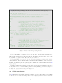
The function EXAMPLE 1 synthetic 2D data demonstrate the use of uncertainty learning for the
purpose of classifiying synthetic data. As can be seen on Figure 3, it mainly consists in training
and testing phases for each classes using the proposed approach (Uncertainty training on noisy
data) and conventional ones (Conventional training on clean or noisy data).
The Figure 4 gives a sense of the results for a 2-dimensional case.
3
function EXAMPLE_1__synthetic_2D_data ()
% comments and g e n e r a t i o n o f s y n t h e t i c d a t a
...
for train_mode = train_modes
%d i s p l a y i n f o
...
% TRAIN
% −−−−−−−−−−−−−−−−−−−−−−−−−−−
f o r cl = 1 : n b C l a s s e s
f p r i n t f ( ' T r a i n model %d o f %d models \n ' , cl ,
nbClasses ) ;
x _ n o i s y _ t r a i n _ c l = s q u e e z e ( x _ t r a i n _ C U R ( cl , : , : ) ) ;
c E _ t r a i n _ c l = s q u e e z e ( c E _ t r a i n _ C U R ( cl , : , : ) ) ;
[ uXe , c X e ] = V Q ( x _ n o i s y _ t r a i n _ c l ,
covariances
log2 ( nbGaussians ) , 0) ;
% 0:
initialize
f u l l ←-
wXe = ones (1 , nbGaussians ) ;
w X e = w X e /sum ( w X e ) ;
[ e s t _ g m m s { t r a i n _ m o d e , c l } . u _ g m m , e s t _ g m m s { t r a i n _ m o d e , c l } . c _ g m m , e s t _ g m m s {←train_mode , cl } . w_gmm ] = . . .
G M M _ E M _ u n c e r t a i n t y _ l e a r n i n g ( x _ n o i s y _ t r a i n _ c l , c E _ t r a i n _ c l , uXe , cXe , wXe , ←[ ] , 0 ) ; % 0 : no l o g
end ;
% TEST
% −−−−−−−−−−−−−−−−−−−−−−−−−−−
log_likelihoods = zeros ( nbClasses , nbSequences_test ,
f o r cl = 1 : n b C l a s s e s
f p r i n t f ( ' T e s t f o r c l a s s %d o f %d c l a s s e s \n ' , cl ,
nbClasses ) ;
nbClasses ) ;
f o r seq = 1 : nbSequences_test
for cl_model = 1: nbClasses
[ d u m m y 1 , d u m m y 2 , d u m m y 3 , d u m m y 4 , l o g _ l i k e l i h o o d s ( cl , seq , c l _ m o d e l ) ] = ←...
G M M _ E M _ u n c e r t a i n t y _ l e a r n i n g ( s q u e e z e ( x _ n o i s y _ t e s t ( cl , seq , : , : ) ) , ←s q u e e z e ( c E _ t e s t ( cl , seq , : , : ) ) , . . .
e s t _ g m m s { t r a i n _ m o d e , c l _ m o d e l } . u _ g m m , e s t _ g m m s { t r a i n _ m o d e , c l _ m o d e l } . ←c _ g m m , e s t _ g m m s { t r a i n _ m o d e , c l _ m o d e l } . w _ g m m , 1 , 0 ) ; % 0 : no l o g
end ;
end ;
end ;
% compute s c o r e
...
end ;
% visualization
...
Figure 3: Code of the experiment on synthetic data.
4
Speaker recognition experiment on Speech Data
In order to experiment with a more realistic task, we considered in [2], a speaker recognition task
on noisy speech data. In this case, the uncertainty is not know as a prior, and estimated using a
method based on Wiener filtering and Vector Taylor Series (VTS) expansion, see Section 4.1.5 of
[2] for more details.
4
Data GMMs
Noisy data
6
Clean data
6
GMM of class 1
GMM of class 2
GMM of class 3
4
6
Class 1
Class 2
Class 3
4
4
2
2
2
0
0
0
−2
−2
−2
−4
−5
0
5
10
−4
−5
Conventional training, clean data
0
5
10
−4
Conventional training, noisy data
6
6
4
4
4
2
2
2
0
0
0
−2
−2
−2
−5
0
5
10
−4
−5
0
5
0
5
10
Uncertainty training, noisy data
6
−4
−5
10
−4
−5
0
5
10
Figure 4: GMMs estimated using different learning conditions. By considering the uncertainty in
the learning algorithm, the resulting GMMs are much closer to the original ones when considering
noisy data.
4.1
Data
The data is provided separately from this toolbox and can be freely obtained at http://www.
irisa.fr/metiss/ozerov/Software/SP_REC_Uncrt_MFCC.zip. It consists of Mel Frequency Cepstral Coefficients (MFCCs) computed over 3 different inputs:
1. mix: raw addition of clean speech and noise
2. ssep: output of a state of the art source separation algorithm fed with the raw addition of
clean speech and noise
3. ssep uncrt: same, but with an estimate of the uncertainty of the output done with the VTS
method
Details about how and on what kind of audio data the MFCCs have been generated is provided
in Section 4.1.2 of [2].
Data is provided as .MAT file that can be opened with Matlab® or any parser that can read
HDF5 files. The naming convention is as follows: s<speakerId> <utteranceId> mfcc.mat. The
speakerId corresponds to the numeric id of the speaker from 1 to 34. For the 3 different inputs
described above, the .MAT file contains the mfcc variable which is a 2 dimensional floating point
matrix of size 20 × nf , where nf is the number of frames that have been considered for computing
the 20 dimensional MFCCs. For the last input, a second variable mfcc covar is available. It
encodes the uncertainty as a 3 dimensional tensor of size 20 × 20 × nf .
5
The data is divided in two main directories (test and train) that respectively contains the data
used for training and testing. For each one, clean (no noise addition) and several Signal to Noise
ratios are considered from -6dB to 9dB of SNRs. For each SNR, the 3 above discussed conditions
(mix, ssep, ssep uncrt) are available. For the latter, the full covariance uncertainty estimated
using the Wiener / VTS approach is provided. It shall be noted that the MFCCs of this condition
are the same as in the ssep condition as the VTS estimator does not change the actual MFCC
values, see Equation C.2 in [2].
4.2
Code
The function EXAMPLE 2 real 19D MFCC data can be considered to replicate the full results of the
experiments reported in Table D.7 of [2]. One run computes the results for one training/testing
condition for the following 4 cases:
1. Conventional training / Conventional decoding without signal enhancement
2. Conventional training / Conventional decoding with signal enhancement
3. Conventional training / Uncertainty decoding with signal enhancement
4. Uncertainty training / Uncertainty decoding with signal enhancement
Figure 5 shows the first line of the function that set the main processing parameters:
• data dir name: path to the data repository
• speaker ids: selection vector for the speaker to consider. 1 : 34 will consider all the speakers
available
• subdir name test: SNR condition for training from ’m6dB’ (-6 dB SNR) to ’9dB’ (9 dB
SNR), and ’clean’ (∞ SNR)
• subdir name train: SNR condition for testing
On a standard 2 GHz machine with one core, the example shown on Figure 5 with 3 speakers
needs about an hour. The evaluation of one training/testing condition (for example -9dB SNR at
training and 0 dB SNR at testing) is expected to take one day for the 34 speakers available. So,
replicating the results of the full table is expected to take about 48 days.
References
[1] A. Ozerov, M. Lagrange, and E. Vincent, “GMM-based classification from noisy features,” in
Proc. 1st Int. Workshop on Machine Listening in Multisource Environments (CHiME), Florence, Italy, September 2011, pp. 30–35.
[2] ——, “Uncertainty-based learning of gaussian mixture models from noisy data,” Computer
Speech and Language, 2011, submitted.
[3] A. P. Dempster, N. M. Laird, and D. B. Rubin., “Maximum likelihood from incomplete data
via the EM algorithm,” Journal of the Royal Statistical Society. Series B (Methodological),
vol. 39, pp. 1–38, 1977.
6
function EXAMPLE_2__real_19D_MFCC_data ()
% comments
....
d a t a _ d i r _ n a m e = ' . . / SP REC Uncrt MFCC/ ' ;
speaker_ids = [2 , 4 ,
6];
s u b d i r _ n a m e _ t e s t = 'm6dB ' ;
s u b d i r _ n a m e _ t r a i n = 'm6dB ' ;
% can be any from 1 t o 34
% can be ' 0 dB ' ,
% can be ' 0 dB ' ,
' 3 dB ' ,
' 3 dB ' ,
' 6 dB ' ,
' 6 dB ' ,
' 9 dB ' ,
' 9 dB ' ,
'm3dB ' ,
'm3dB ' ,
Figure 5: Main parameters of the speaker recognition task.
7
'm6dB '
'm6dB '