1
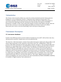
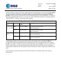
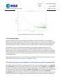
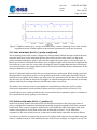
Project: Cluster Active Archive Doc. No. Issue: Date: CAA-‐EST-‐UG-‐EFW 3.1 2011-‐04-‐28 Page: 1 of 26 User Guide to the EFW measurements in the Cluster Active Archive (CAA) prepared by Per-‐Arne Lindqvist Chris Cully Yuri Khotyaintsev and the EFW team Project: Cluster Active Archive Doc. No. Issue: Date: CAA-‐EST-‐UG-‐EFW 3.1 2011-‐04-‐28 Page: 2 of 26 1 Introduction The Cluster Active Archive (CAA) was created to archive all data from the Cluster mission. Emphasis is on providing the scientific community with calibrated science data. This document describes the CAA data from the Electric Field and Waves (EFW) instrument. It gives some brief information on the instrument, followed by a description of all EFW parameters available in CAA. Some important things to keep in mind when using the data are given in the sections on caveats and quality parameters (sections 4 and 5). For those interested, there is also a section describing some of the processing details. 2 Instrument Description 2.1 Instrument hardware Details of the EFW instrument can be found in Gustafsson et al. [1997, 2001]. Here some key characteristics useful for regular users are described briefly. The detector of the instrument consists of four spherical sensors deployed orthogonally on 44 meter long wire booms in the spin plane of the spacecraft. The configuration of the four probes of the EFW instrument in the spin plane is shown in Figure 1. The potential difference between two opposing sensors, separated by 88 m tip-‐tip, is measured to provide an electric field measurement. Since there are four sensors, the full electric field in the spin plane is measured. The potential difference between each sensor and the spacecraft is measured separately (and is often used as a high time-‐resolution proxy for the ambient plasma density, [cf. Pedersen et al., 2008]). The potentials of the spherical sensor and nearby conductors (the so-‐called pucks and guards) are actively controlled in order to minimize errors associated with photoelectron fluxes to and from the spheres. The output signals from the spherical sensor preamplifiers are also provided to the wave instruments (STAFF, WHISPER and WBD) for analysis of high frequency wave phenomena. Project: Cluster Active Archive Doc. No. Issue: Date: CAA-‐EST-‐UG-‐EFW 3.1 2011-‐04-‐28 Page: 3 of 26 Figure 1. EFW probe configuration. 2.2 Probes and filters EFW measures individual probe potentials with respect to the spacecraft with a sampling frequency of 5 s-‐1, as well as the potential difference between selected probe pairs with a sampling frequency of 25 s-‐1 or 450 s-‐1 depending on the spacecraft telemetry mode [this can be seen in TMMODE dataset]. Normally, the full spin plane electric field is computed using the orthogonal signals p12=p2-‐
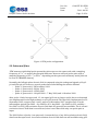
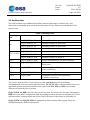
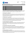
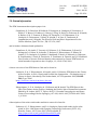
p1 and p34=p4-‐p3. However, several probes have failed during the mission lifetime: − probe 1, spacecraft 1: 28 December 2001 − probe 1, spacecraft 3: 29 July 2002 − probe 1, spacecraft 2: 13 May 2007 − probe 4, spacecraft 1: 19 April 2009 – 7 May 2009, and 14 October 2009 After probe 1 failed on spacecraft 1-‐3, the signal p12 was no longer useful, but a workaround was implemented in the flight software to use p32 instead. This was fully implemented on 29 September 2003 on spacecraft 1 and 3, and on 24 November 2007 on spacecraft 2. In the intermediate period (Jan 2002 – Sep 2003 for SC1, Aug 2002 – Sep 2003 for SC3, and May – Nov 2007 for SC2), full resolution electric field data are generally not available. The 4-‐second resolution electric field data is not affected, since it uses data from only one probe pair as input. The 2009 failure of probe 4 on spacecraft 1 meant the loss of any full resolution electric field data from that spacecraft. 4-‐second resolution electric field data was still available using p32. Project: Cluster Active Archive Doc. No. Issue: Date: CAA-‐EST-‐UG-‐EFW 3.1 2011-‐04-‐28 Page: 4 of 26 A schematic overview of the relevant signal paths is given in Figure 2. The individual probe signals, p1 to p4, are normally routed through 7-‐pole low-‐pass filters with a cut-‐off frequency of 10 Hz before sampling. The probe difference signals, p12, p34 and p32 are normally routed through 10 Hz low-‐pass filters if sampled at 25 s-‐1, and through 180 Hz low-‐pass filters when sampled at 450 s-‐1. The filters are normally connected to the sampled quantities as indicated in Figure 2. However, the 10 Hz filter on probe 3 on spacecraft 2 failed on 25 July 2001. As a workaround for this, the 180 Hz filter has been used for the difference signals sampled at both 450 s-‐1 and 25 s-‐1. From 1 June 2007, all single probe signals on this spacecraft also use the 180 Hz filters. This has no effect on the 4 second resolution data, and only a marginal effect on the 25 s-‐1 data in those space environments where large amplitude electric field noise is present between 10 and 180 Hz. Figure 2. Probes, filters and sampled quantities Project: Cluster Active Archive Doc. No. Issue: Date: CAA-‐EST-‐UG-‐EFW 3.1 2011-‐04-‐28 Page: 5 of 26 2.3 Summary of operations Table 1 gives an overview of the operations of the EFW probes on the four spacecraft. The user should be aware that the full resolution (Level 2) electric field data are affected by the number of probes available for E-‐field measurements. With only 2 probes the despun electric field will have a large spin variation and is of limited use. With 3 probes the despun electric field will have some spin variation, depending on the plasma environment. The quality indicators for the Level 2 electric field data are set accordingly; see section 5. Table 1. Operational status of the EFW experiment Spacec Time period Number of E- Raw E-field Quality, full-
raft field probes signals resolution available available electric field data SC1 2001-‐02-‐01 – 2001-‐12-‐28 4 p12 and p34 3 2001-‐12-‐28 – 2003-‐09-‐29 2 p34 only 1 2003-‐09-‐29 – 2009-‐04-‐19 3 p32 and p34 2 2009-‐04-‐19 -‐ 2 p32only 1 2009-‐05-‐07 2009-‐05-‐07 -‐ 3 p32 and p34 2 2009-‐10-‐14 2009-‐10-‐14 -‐ 2 p32only 1 present SC2 2001-‐02-‐01 – 2007-‐05-‐13 4 p12 and p34 3 2007-‐05-‐13 – 2007-‐11-‐24 2 p34 only 1 2007-‐11-‐24 – present 3 p32 and p34 2 SC3 2001-‐02-‐01 – 2002-‐07-‐29 4 p12 and p34 3 2002-‐07-‐29 – 2003-‐09-‐29 2 p34 only 1 2003-‐09-‐29 – present 3 p32 and p34 2 SC4 2001-‐02-‐01 – present 4 p12 and p34 3 Project: Cluster Active Archive Doc. No. Issue: Date: CAA-‐EST-‐UG-‐EFW 3.1 2011-‐04-‐28 Page: 6 of 26 2.4 Measurement calibration and processing In processing the EFW data for the CAA, the EFW team uses a combination of ground and in-‐
orbit calibrations. The in-‐orbit calibrations incorporate extensive cross-‐calibration with other instruments and inter-‐calibration between the 4 satellites. Further information is contained in the CAA-‐EFW Calibration Report and Appendix A below. 3 Data sets 3.1 Choosing which data set to use As of May 2010, there were a total of 22 different EFW data products. This section is written to help users select the appropriate data product. Essentially, the choice boils down to 2 or 3 questions: 1. Are you interested in spacecraft potential measurements, electric field measurements, ExB drift velocities or something else (non-‐science)? 2. What measurement cadence do you want (full resolution or 4 second resolution)? 3. For electric field measurements, what frame do you want? The answer to the first question should be obvious. The second and third questions, on the other hand, may be more subtle than they look. When selecting the cadence, keep in mind that the spin period of the spacecraft is roughly 4 seconds, and we take care to do the averaging in such a way as to always take any detected errors into consideration when we process the 4 second resolution data. In general, unless you really need resolution better than 4 seconds, the EFW team always recommends the 4-second resolution data. The period of exactly 4 seconds was chosen rather than locking the timing to the spin period in order to make longer-‐duration spectral studies possible. The user must always keep in mind that EFW only measures 2 components of the electric field, and also that the sunward component has a larger DC measurement uncertainty. Rotation away from the measurement frame (e.g. rotation to GSE) is inherently a 3D operation, and may therefore introduce systematic errors. The natural coordinate system for EFW data is the ISR2 data system. The EFW team therefore recommends the ISR2 frame for most analysis. Data in GSE coordinates should be used only if truly required for the analysis. This is discussed in more detail in section 3.6. 3.2 Science data: spacecraft potential The science dataset for the spacecraft potential is listed in table 2. The CAA dataset names are all prefaced with “C[n]_CP_EFW_ “, where n is the spacecraft number. See section 4.1 for recommendations and caveats regarding spacecraft potential measurements. Table 2. Science data: spacecraft potential Project: Cluster Active Archive Doc. No. Issue: Date: CAA-‐EST-‐UG-‐EFW 3.1 2011-‐04-‐28 Page: 7 of 26 Sampling rate CAA Dataset name Description 5 s-‐1 L2_P Spacecraft potential (0.2 sec resolution) 0.25 s-‐1 L3_P Spacecraft potential (4 sec resolution) L2_P and L3_P are the average potential of all available probes, measured relative to the spacecraft. If all four probes are available, the average is done over all 4 probes. If only two or three probes are available, the average is done over 2 probes (P1 and P2, or P3 and P4). If only one probe is available, this quantity is the value of that probe. The probes used are given by the parameter P_probes. When moderate high-‐bias saturation is detected on one of the probes (indicated by bit 14 in the P_bitmask), the average over 4 seconds is replaced by a maximum over 4 seconds to avoid errors resulting from the resulting spikes (see section 4.1.4); also the data quality is lowered for such intervals. The individual probe potentials are available in the ancillary data. 3.3 Science data: electric field The science datasets for the electric field are listed in table 3. All electric field datasets include quality indicators (see section 5). Users must check the quality indicators before using any electric field data product. For help on choosing an appropriate frame, see section 3.6. The CAA dataset names are all prefaced with “C[n]_CP_EFW_ “, where n is the spacecraft number. The sampling rate of the electric field measurements can vary in the full-‐resolution datasets depending on the spacecraft telemetry mode; to find the spacecraft telemetry mode, see CAA Auxiliary (Dataset name: “Telemetry Mode”). Table 3. Science data: electric field Sampling rate Frame CAA Dataset name Dataset title 0.25 s-‐1 ISR2 L3_E 2D Electric field, (4 sec resolution)* ISR2, inertial L3_E3D_INERT 3D Electric field in ISR2 (E.B=0) (4 sec resolution) GSE, inertial L3_E3D_GSE 3D Electric field in GSE (E.B=0) (4 sec resolution) L2_E 2D Electric field (full resolution)* L2_E3D_INERT 3D Electric field in ISR2 (E.B=0) (full resolution) ISR2 -‐1
25 s or 450 ISR2, s-‐1 inertial GSE, L2_E3D_GSE 3D Electric field in GSE (E.B=0) inertial (full resolution) * this dataset is available as ancillary dataset L3_E is the electric field vector (Ex and Ey) in the spin plane, computed from a least-‐squares fit of a sine wave to one probe pair (P12 or P34) over 4 seconds (approximately one spin). Project: Cluster Active Archive Doc. No. Issue: Date: CAA-‐EST-‐UG-‐EFW 3.1 2011-‐04-‐28 Page: 8 of 26 The least-‐squares fit is normally done on P34, if available, otherwise on P12. The result is two components of the electric field (Ex and Ey) and a measure of the standard deviation of the raw data points from a sine wave, Sigma (proxy for wave power at higher frequencies). Also included in this dataset are quality indicators E_quality and E_bitmask (see section 5). This data is in the ISR2 (instrument) coordinate system (see section 3.6) and forms the basis from which the other L3 data sets are calculated. L3_E3D_INERT is the electric field vector in the spin plane in the inertial reference frame. It is computed from L3_E by first subtracting the spacecraft motion induced electric field vsc x B, and then computing the third (non-‐measured axial) component of the electric field using the assumption E.B = 0. These computations are done at the CAA using the FGM CAA 5VPS dataset. The third component is only computed when the magnetic field direction is more than 15 degrees away from the spin plane and | BZ | is larger than 2 nT (otherwise the error in the third electric field component becomes too large). If this restriction is not met, then fill values are inserted in the third component. An error estimate for the third component is also provided. L3_E3D_INERT is the preferred data product for most analysis. If using the third component, one should always keep in mind that it is artificially constructed and not actually measured. L3_E3D_GSE is the full 3-‐dimensional electric field vector in the GSE coordinate system. It is computed from L3_E3D_INERT by rotating from the ISR2 coordinate system to the GSE system. This rotation mixes together the two measured components with the third (unmeasured) component. This product is only available when the third component can be constructed, and may therefore contain long intervals of fill data when the magnetic field is near the spin plane or when | BZ | becomes small. Since the assumption E.B = 0 is used in the creation of this dataset, the GSE electric field is perpendicular to B by construction. L2_E is the electric field vector (Ex and Ey) in the spin plane, computed using as many probes as available. It is in the ISR2 (instrument) coordinate system (see section 3.6) and is the basis from which the other L2 data sets are calculated. L2_E3D_INERT is computed from L2_E in the same manner as L3_E3D_INERT is computed from L3_E (see above). L2_E3D_INERT is the preferred data product for analysis requiring full-resolution data. If using the third component, one should additionally be aware that the assumption E.B = 0 may not be valid at higher frequencies. L2_E3D_GSE is computed from L2_E3D_INERT in the same manner as L3_E3D_GSE is computed from L3_E3D_INERT (see above). In addition to the problems listed above under L3_E3D_GSE, the assumption E.B = 0 may not be valid at higher frequencies. Users are encouraged to consider the other electric field data sets if at all possible. 3.4 Science data: ExB drift velocities The science dataset for the ExB drifts are listed in table 4. These data sets contain the plasma convection flow velocity, computed from E3D_INERT and the magnetic field B as VGSE = (EGSE x B) / B2. The FGM CAA 5VPS dataset has been used here for 4-‐sec datasets and the FGM Full-‐resolution dataset for full-‐resolution drift velocity datasets. All drift datasets include Project: Cluster Active Archive Doc. No. Issue: Date: CAA-‐EST-‐UG-‐EFW 3.1 2011-‐04-‐28 Page: 9 of 26 quality indicators derived from the underlying electric field data (see section 5). Users must check the quality indicators E_quality and/or E_bitmask before using any ExB data product. These quality indicators are also included in the drift velocity datasets. For help on choosing an appropriate frame, see section 3.6. The CAA dataset names are all prefaced with “C[n]_CP_EFW_ “, where n is the spacecraft number. Table 4. Science data: ExB drift velocities Sampling rate Frame CAA Dataset name Description ISR2 25 s-‐1 or 450 s-‐1 GSE L2_V3D_INERT ExB drift velocity in ISR2 (full resolution) L2_V3D_GSE ExB drift velocity in GSE (full resolution) 0.25 s-‐1 ISR2 L3_V3D_INERT ExB drift velocity in ISR2 (4 sec resolution) GSE L3_V3D_GSE ExB drift velocity in GSE (4 sec resolution) Computing the drift velocity in any frame inherently requires the assumption E.B=0 to construct the unmeasured third (axial) component of E. This computation in turn requires that B is more than 15 degrees away from the spin plane and that |B| > 2 nT (see section 3.3). If this restriction is not met, then the drift velocity data will contain fill values except the z component in ISR2 that can calculated from the measured x and y components of the electric field. All convection velocities are given in an inertial frame (i.e. with the spacecraft velocity subtracted). Project: Cluster Active Archive Doc. No. Issue: Date: CAA-‐EST-‐UG-‐EFW 3.1 2011-‐04-‐28 Page: 10 of 26 3.5 Ancillary data The CAA contains some additional ancillary data sets that may be useful to the user interested in minimally-‐processed or historical data. These data are not intended for the general user. Table 5. Ancillary data Sampling rate CAA Dataset name Description 5 s-‐1 C[n]_CP_EFW_L1_P1 Potential, Probe 1 to spacecraft C[n]_CP_EFW_L1_P2 Potential, Probe 2 to spacecraft C[n]_CP_EFW_L1_P3 Potential, Probe 3 to spacecraft C[n]_CP_EFW_L1_P4 Potential, Probe 4 to spacecraft C[n]_CP_EFW_L1_P12 -‐1
25 s or 450 C[n]_CP_EFW_L1_P32 s-‐1 C[n]_CP_EFW_L1_P34 Potential, Probe 1 to Probe 2 0.25 s-‐1 C[n]_CP_EFW_L3_DER Electric Field offsets (4 second resolution) 0.25 s-‐1 C[n]_CP_EFW_L3_SFIT Spinfits of the electric field from the individual probe pairs 0.25 s-‐1 C[n]_PP_EFW Preliminary Electric Field parameters (4 sec resolution) 1/32 s-‐1 C[n]_CP_EFW_L2_HK Instrument settings 1/60 s-‐1 C[n]_SP_EFW Preliminary Electric Field parameters (1 minute resolution) Potential, Probe 3 to Probe 2 Potential, Probe 3 to Probe 4 The Level 1 datasets (first 7 rows above) are the raw data from the instrument, decommutated and converted to physical units. P1, P2, P3, P4 are the potentials of the four individual probes, measured relative to the spacecraft. P12, P34 and P32 are potential differences between pairs of probes. C[n]_CP_EFW_L3_DER is the DC offset in the raw data. See section 6.1 for more information. DER is a vector with 2 components and, depending on which probes are available for E-‐field measurements, contains either the offsets in p12 and p34 or the offsets in p32 and p34. C[n]_PP_EFW and C[n]_SP_EFW are preliminary data from the CSDS system. They are included mostly for historical purposes. Project: Cluster Active Archive Doc. No. Issue: Date: CAA-‐EST-‐UG-‐EFW 3.1 2011-‐04-‐28 Page: 11 of 26 3.6 Coordinate systems The EFW instrument measures the electric field only in the spacecraft spin plane. The preferred coordinate system for scientific studies involving the electric field is therefore a spin-‐plane oriented coordinate system. The ISR2 (Inverted Spin Reference) system, also known as DSI (Despun System Inverted), is such a system. The x-‐axis is in the spin plane and pointing as near sunward as possible. The y-‐axis is in the spin plane, perpendicular to the sunward direction, positive towards dusk. The z-‐axis is along the (negative) spacecraft spin axis, positive towards the north ecliptic. [The coordinate system is called “Inverted” because Cluster is actually “inverted” with the spin axis pointing towards the south ecliptic.] The difference between ISR2 (DSI) and GSE (Geocentric Solar Ecliptic) is primarily a rotation of between 2 and 7 degrees around the y-‐axis, which is due to the fact that the spacecraft is slightly tilted so as not to shadow the EFW probes. In the intervals between attitude adjustments on the spacecraft, a very small rotation can also be present about the x axis. The one major exception was during the May 2008 “tilt campaign”, when the spin axis of C3 was deliberately tilted by up to 45 degrees about the x axis. Between 09:00 UT on 2008-‐04-‐25 and 08:24 UT on 2008-‐05-‐30, the ISR2 and GSE systems therefore differ substantially on C3. 4 Recommendations and caveats Much effort has been spent on calibrating the data and removing spurious effects to give a useful database for scientific analysis. In spite of this, there will be data in the CAA which are not of optimum quality. It is important that anyone using the EFW CAA data be aware of the pertinent measurement issues to avoid misinterpretations of the data. 4.1 Spacecraft potential There are point-‐by-‐point quality flag and bitmask attached to the spacecraft potential data, as there is for the electric field data (see section 5). This section therefore describes some of the problems of which the user should be aware. 4.1.1 ASPOC operations The ASPOC instrument attempts to keep the spacecraft potential at a low value, primarily to enable low-‐energy ion and electron measurements by the particle instruments. In the absence of ASPOC the spacecraft potential often reaches several tens of V in the low-‐density plasmas encountered by Cluster. With ASPOC operating, the spacecraft potential is brought down to the order of 5-‐8 V. A positive side-‐effect of this is that the electric field measurements are most often improved since the wake effects associated with large spacecraft potentials in the polar cap (see section 5.12) are drastically reduced. The spacecraft potential is often used as a proxy for ambient plasma density variations (see Pedersen et al., 2008). Any use of the spacecraft potential to determine plasma density should take into account whether ASPOC was operating or not, which is indicated by the ASPOC_status parameter included with L2/3_P. ASPOC is not operational on spacecraft 1. Due to the end of Indium ions, ASPOC operations were stopped in 2006 (TBC) on other spacecraft. Project: Cluster Active Archive Doc. No. Issue: Date: CAA-‐EST-‐UG-‐EFW 3.1 2011-‐04-‐28 Page: 12 of 26 4.1.2 EDI operations EDI measures the ambient electric field by emitting a beam of electrons and detecting the drift step as the electrons gyrate around the ambient magnetic field. The emitted beam current contributes to increasing the spacecraft potential, and the effects can be particularly large in a low density plasma. During some periods in the beginning of the mission, the emitted EDI beam current was larger than expected, in particular on Cluster 2, so there is a tendency for the spacecraft potential to be larger than on the other spacecraft. Since the spacecraft potential is often used as a proxy for a measurement of the ambient plasma density, this could be misinterpreted as a lower density at Cluster 2. This problem was alleviated in 8 April 2004, when the EDI guns on C2 were turned off in favour of running the instrument in an alternative “ambient” mode. Normal EDI operations also affect the potential somewhat, especially when run in the high beam current mode. In later years (after about 2004), the potentials on C1 and C3 (where EDI is run) are often notably different from the potentials on C2 and C4 in the same plasma environment. 4.1.3 Whisper operations The WHISPER instrument regularly emits waves using the EFW probes to detect resonances frequencies in the ambient plasma. There are some remaining effects at the start and end edge of the active sounding periods, mainly seen as small spikes in the Level 3 potential data [see CAA-‐EFW-‐ICD-‐0001, appendix 5, for details]. The WHISPER active soundings are done regularly, often at a repetition period of 52 s or 104 s, so they should be easy to separate from real variations in the data. The soundings are also marked in the EFW spacecraft potential and electric field data (bit 13 in the P_bitmask , also see section 5.14) 4.1.4 High bias saturation The EFW instruments draw a bias current from the plasma in order to anchor the probes to the local plasma potential. If this bias current is too large, then the probes behave extremely non-‐linearly and shoot to large negative potentials (“saturate”). This happens on occasion when the plasma density is high. Moderate saturation results in spikes in the potential whenever the affected probe points sunward, while full saturation sends the probes to their minimum value of -‐68 Volts. The problem was worse in 2005 and early 2006, and was largely eliminated by a change in the bias settings on 2006-‐06-‐16 (see the CAA EFW Calibration Report). The processing software automatically detects high bias saturation intervals on a probe-‐by-‐
probe basis. The affected intervals are indicated by bit 14 in the P_bitmask. When a problem with high bias saturation is detected, data from severely affected probes (those that reach -‐68 Volts) is first discarded, and then the L2 and L3 data are computed from the maximum potential of the remaining operational probes. By using the maximum value instead of the mean value, the data is only slightly affected when one probe spikes toward large negative values. Since only one probe at a time can point in the sunward direction, the resulting timeseries does not exhibit the large spikes in the underlying signals. Project: Cluster Active Archive Doc. No. Issue: Date: CAA-‐EST-‐UG-‐EFW 3.1 2011-‐04-‐28 Page: 13 of 26 Spin variations in the spacecraft potential are a real and expected effect resulting from the changing photoemissive area of the spacecraft. However, large (> 5V) spin-‐synchronous spikes in L2_P in a high density environment (L3_P > -‐10 V) should be treated as suspicious. Check whether high bias saturation was detected by checking bit 15 of E_bitmask for electric field data during the interval. 4.1.5 Spacecraft-‐to-‐plasma potential The “spacecraft potential” in the CAA-‐EFW data products reflects the potential of the biased probes with respect to the spacecraft. This is not exactly the same as the potential of the spacecraft with respect to the plasma. First of all, note the sign convention: the Cluster spacecraft are usually positive with respect to the plasma, so the probe-‐to-‐spacecraft potential data in the CAA is typically negative. Second, the probes typically also float somewhat positive with respect to the plasma, but at a very much smaller potential than the satellite (roughly 1 V, as compared to up to >70 V). Third, the probes are affected by the potential on the long wire booms, and hence the true spacecraft-‐to-‐plasma potential may be somewhat larger (up to 23% in tenuous plasmas). Users who require the spacecraft-‐to-‐
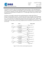
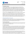
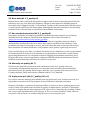
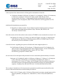
plasma potential are referred to Cully et al [2007] and Pedersen et al [2008]. 4.2 Electric field data All EFW data in the CAA has a quality parameter attached to it. Users must check this quality parameter before using the data. The quality parameters are described in section 5; this section describes other general caveats that are not specifically flagged. 4.2.1 Instrument noise level The EFW electronics are optimized primarily for lower frequencies and larger amplitudes. However, some users may be interested in very weak AC signals, for example for turbulence studies. For such applications, the user should be aware of the AC instrument noise, which may become visible in the 450 Hz data. Figure 3 shows an example of data which reaches the AC noise floor. The noise above a few tens of Hz is set by interference from nearby digital electronics, which causes fluctuations in the electrical ground level. At higher frequencies, there is a roughly white component, plus some discrete lines. The exact spectral density may vary slightly from event to event. The EFW noise is discussed in more detail in the CAA-‐EFW Calibration Report. Project: Cluster Active Archive Doc. No. Issue: Date: CAA-‐EST-‐UG-‐EFW 3.1 2011-‐04-‐28 Page: 14 of 26 Figure 3: Noise floor as seen in the 450 Hz data. 4.2.2 Sunward offsets Double-‐probe electric field experiments like EFW are affected by offsets in the sunward direction, caused by asymmetries in the photoelectron emission. The electric field data in the CAA has been corrected for this effect by cross-‐calibrating the measured electric fields with other instruments, and then subtracting a DC sunward offset, as discussed in Appendix B. The offset is, however, somewhat dependent on the ambient plasma parameters. We therefore use different offsets in the solar wind and magnetosheath as compared to the magnetosphere. These offsets may differ by a few tenths of a mV/m. Furthermore, the offsets in the solar wind are affected by the solar wind parameters: the sunward offsets are smaller in the high-‐speed solar wind). More information on the offsets can be found in the CAA_EFW Calibration Report. Although relative deviations of a few mV/m can usually be trusted, the uncertainty in the DC offset limits the absolute DC accuracy to roughly 1 mV/m. 5 Quality parameters for theelectric field and spacecraft potential data Each EFW electric field dataset contains the same two record-‐varying parameters: E_quality and E_bitmask. For the spacecraft potential these parameters are P_quality and P_bitmask. These are computed automatically by the processing software and help the user to filter out scientifically poor-‐quality data values. E_quality (P_quality) can be used as a general guide as to whether a given data interval is appropriate for publication, while the E_bitmask (P_bitmask) supplies details as to exactly which problems may be present. Users must check these parameters before using any spacecraft potential, electric field or drift velocity data. Project: Cluster Active Archive Doc. No. Issue: Date: CAA-‐EST-‐UG-‐EFW 3.1 2011-‐04-‐28 Page: 15 of 26 Keep in mind that the quality flags are determined automatically. While they are generally quite robust and further verified manually, they are by no means infallible. E_bitmask (P_bitmask) is a binary bit mask indicating various types of problems associated with the data. The meaning of the bits are as follows, and are explained in more detail in the subsections below. Table 6. Meaning of the E_bitmask and P_bitmask flags. Bit Decimal Meaning E_quality P_quality value <= <= 0 1 Reset 0 1 1 2 Bad bias 0 1 2 4 Probe saturation 0 1 3 8 Low density saturation (-‐68V) 0 1 4 16 Sweep (collection and dump) 0 N/A 5 32 Burst dump 0 N/A 6 64 Non-‐standard operations (NS_OPS) 0 N/A 7 128 Manually set E_quality N/A N/A 8 256 Single probe pair (affects only Level 2 data) 1 (L2 only) N/A 9 512 Asymmetric mode (p32 and p34, affects only 2 (L2 only) N/A Level 2 data) 10 1024 Solar wind wake correction applied 3 N/A 11 2048 Lobe wake 1 N/A 12 4096 Plasmaspheric wake 1 N/A 13 8192 Whisper operating 2 0 14 16384 Saturation due to high bias current 1 2 15 32768 Not used N/A N/A The resulting value of the bitmask is a binary OR of all the relevant values. For example, if a plasmaspheric wake (bit 12) is detected at the same time as Whisper is operating (bit 13), then the resulting bitmask is 2¹²+2¹³= 12288. In Matlab this can done using function bitand(): >> mask=12288;
>> for bit=0:15, if (bitand(mask, 2^bit)),...
fprintf('Bit #%d set\n',bit), end, end
Bit #12 set
Bit #13 set
>>
E_quality (P_quality) gives the estimated quality of the electric field (spacecraft potential). Possible values are as follows: Project: Cluster Active Archive Doc. No. Issue: Date: CAA-‐EST-‐UG-‐EFW 3.1 2011-‐04-‐28 Page: 16 of 26 Table 7. E_quality and P_quality definitions. Quality Meaning 0 Bad data 1 Known problems, use at your own risk 2 Survey data, possibly not publication-‐quality 3 Good for publication, subject to PI approval 4 Excellent data which has received special treatment Except in rare circumstances when E_quality is set manually, it is taken as the lowest quality associated with any identified problem. So in the above example with plasmaspheric wake (E_quality<=1) and Whisper operation (E_quality<=2), E_quality would be 1. 5.1 Reset (bit 0, E_quality=0) When the EFW instrument is first initialized after an on-‐orbit reset (usually twice per orbit), it takes a few moments before the instrument begins operating in the desired mode. Bit 0 of E_bitmask marks any data transmitted before this set-‐up procedure is complete. These data are generally not useful for any purpose. 5.2 Bad bias (bit 1, E_quality=0) In order to obtain a reliable measurement of DC fields and spacecraft potential, the EFW instrument draws a bias current from the probes. If this bias current is set incorrectly (for example, because of a commanding error), then bit 1 of E_bitmask is set and E_quality is set to zero. Electric field fluctuations at high frequencies (above a few Hz) may or may not be recoverable from these data, and low-‐frequency fields should not be trusted. 5.3 Probe latchup (bit 2, E_quality=0) Occasionally, the EFW probes sometimes become stuck at a fixed voltage, independent of the plasma conditions. This is usually the result of a problem in the digital electronics. Under these conditions, we set bit 2 of E_bitmask. These data points are not useful, and we set E_quality to zero. 5.4 Low density saturation (bit 3, E_quality=0) The EFW electronics is designed to handle spacecraft potentials up to roughly 68 Volts. Beyond this level, the probe potentials saturate and the measured potential differences either become severely distorted (if only one probe saturates) or constant and near-‐zero (if both probes saturate). No meaningful information about the electric field can be extracted from this data. 5.5 Sweep data (bit 4, E_quality=0) Bias current and voltage sweeps are performed at regular intervals (2 hours for most of the mission) and usually last for 9 seconds. These sweeps are useful for probe diagnostics for the EFW team. During these sweeps, there is no electric field data. At the moment, the sweep data is not archived in the CAA in any processed form. Project: Cluster Active Archive Doc. No. Issue: Date: CAA-‐EST-‐UG-‐EFW 3.1 2011-‐04-‐28 Page: 17 of 26 5.6 Burst data (bit 5, E_quality=0) Internal burst data is collected during short triggered intervals and normally placed into the telemetry once per orbit. When the telemetry stream is interrupted for dumping internal burst data, this is flagged with bit 5 of E_bitmask. The data in the internal burst will have been recorded much earlier than the burst dump. Although the internal burst data is not presently archived in the CAA, this data set should become available in the future. 5.7 Non-‐standard operations (bit 6, E_quality=0) Sometimes, problems arise that are outside of normal operations and not covered by the available bits in the bitmask. The EFW team maintains a list of these intervals at: http://www.cluster.irfu.se/efw/ops/ns_ops.html This information is also provided as the EFW caveat dataset (ancillary dataset) which is automatically distributed to the users when they request any EFW science dataset. These problems can range from benign to severe. Intervals when the data is adversely affected by these problems are marked with bit 6 of E_bitmask, and E_quality is generally set to zero. If you see this flag in your data, you should check the list (see link above) or the caveat dataset for further details. In some rare circumstances, the data may be useful after careful further processing. Manoeuvres are a frequent reason for flagging non-‐standard operations, since firing the thrusters creates large plumes of plasma that disturb the measurements. Electric field data acquired during such intervals cannot be corrected. 5.8 Manually-‐set quality (bit 7) Each bit in the bitmask is associated with a maximum value for E_quality. However, occasionally, during manual inspection, we encounter intervals when the automatically-‐
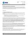
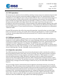
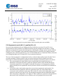
determined value of E_quality doesn't agree with the “true” quality of the data, and we set E_quality by hand. These intervals are marked with bit 7 of E_bitmask. 5.9 Single probe pair (bit 8, E_quality (L2) <=1) For various reasons, data may be available from one probe pair only. In these intervals, it is impossible to measure the 2D spin-‐plane electric field faster than spin resolution. However, the higher-‐resolution L2 data may still be of interest to those studying waves, and so the L2 data is included in the CAA with E_quality no higher than 1 and bit 8 of E_bitmask set. Prior to despin, the missing component of E is put to zero. Naturally, the resulting L2 data has a severe spin modulation as seen in Figure 4. The 4 second resolution L3 data relies on one probe only and hence is unaffected by the lack of a second probe pair. Project: Cluster Active Archive Doc. No. Issue: Date: CAA-‐EST-‐UG-‐EFW 3.1 2011-‐04-‐28 Page: 18 of 26 olution, green) for a period when only one probe pair was available. Fig
ure 4. Co
mp
aris
on of L2 (25 s⁻¹, blu
e) and L3 (4 sec
ond res
5.10 Asymmetric mode (bit 9, E_quality (L2) <=2) Several of the individual electric field probes have failed (see section 2.2 and 2.3). As a workaround for this problem, the EFW instrument can be configured to measure voltage differences that do not involve the failed probe. Labelling the voltages at the 4 probes shown in Figure 1 as V1 through V4, the nominal configuration is to measure the longest-‐baseline orthogonal pairs: (V4-‐V3) and (V2-‐V1). If V1 is unavailable due to a hardware failure, then the non-‐orthogonal pairs (V4-‐V3) and (V3-‐V2) are measured instead. The use of this asymmetric configuration leads to reduced data quality in the L2 data. The 4-‐
second resolution L3 data requires only one probe pair and is hence unaffected. Users interested in L2 data marked as asymmetric mode should be particularly aware of 2 effects. • First, the asymmetric data tends to have considerably more spurious power at harmonics of the spin frequency than the symmetric data. Users should always be extremely suspicious of any signals at the spin frequency or its harmonics, and this applies doubly in the asymmetric mode (for more detail see the EFW CAA Calibration Report). • Second, the solar wind wake cannot be corrected on asymmetric probe pairs. For intervals with one symmetric and one asymmetric pair, the solar wind wake is corrected on the symmetric pair only. This results in a solar wind wake spike once per spin in Ex and once per spin in Ey. The Ex signal sometimes has an additional small lower-‐frequency component, as in Figure 5. These spikes are present in all asymmetric data in the solar wind and are not related to the true geophysical electric field. Project: Cluster Active Archive Doc. No. Issue: Date: CAA-‐EST-‐UG-‐EFW 3.1 2011-‐04-‐28 Page: 19 of 26 Figure 5. High-‐resolution (L2) electric field data from C3 when operating in the solar wind in asymmetric mode. Similar spikes in the nominal (symmetric) mode are removed. 5.11 Solar wind wake (bit 10, E_quality unaffected) The streaming solar wind creates a negatively charged wake behind the spacecraft in the anti-‐
sunward direction. As the individual probes enter and exit this wake, there is a dip in the probe potential, and thus a spike in the raw data signal twice per spin on each probe pair. In the de-‐spun electric field data this shows up as a negative spike in the sunward component Ex, four times per spin, once for each probe entering the wake. An algorithm has been developed to correct for these solar wind wakes in the Level 2 electric field data before submission to the CAA [see Eriksson et al., 2007]. Bit 10 of E_bitmask indicates that this correction has been performed. While doing a good job, the algorithm is not always perfect, so the problem with solar wind wakes should be kept in mind as soon as spikes at four times per spin period are encountered in the data. Users should also be wary of any data in which bit 10 toggles on and off throughout the interval, as this may indicate that the processing software missed some wake corrections. The wake correction procedure is not applied to asymmetric probe pairs (p32), so data collected in asymmetric mode will have spikes twice per spin period (see section 5.10). Provided there are no other problems, the corrected data from symmetric pairs is considered fit for publication, and E_quality is not reduced. 5.12 Cold ion drift wake (bit 11, E_quality<=1) In the low-‐density plasma encountered in the tail lobes and above the polar caps, there is often a cold plasma component streaming essentially along the magnetic field lines, outward from Earth. This creates a negative wake on the anti-‐earthward side of the spacecraft, with similar consequences on the data as the solar wind wake (section 5.11). A difference compared to the solar wind, however, is that the ion drift wake is broader and more diffuse. It is often very hard to recognize the presence of cold ion drift wakes in the raw data since the effect is similar to that of a real ambient electric field. For an example, see Figure 9 in CR. The Project: Cluster Active Archive Doc. No. Issue: Date: CAA-‐EST-‐UG-‐EFW 3.1 2011-‐04-‐28 Page: 20 of 26 CAA production software attempts to detect all such ion wakes by looking at a combination of parameters, such as spacecraft potential, magnetic field direction, and the relation between different electric field components. At present there is no algorithm to correct the data so the bad data are marked with E_quality<=1 and bit 11 in E_bitmask. Since it is sometimes difficult to discern between these wakes and a real electric field, analysis of the electric field should be done with caution in regions where cold plasma ion drift occurs. Keep in mind that the identification is performed automatically and may not always mark the entire interval. Consider User should consider comparing measurements to EDI data, which is not affected. When ASPOC is operating, the spacecraft potential is kept at a much lower value and the problem of wakes due to cold ion drift is much less severe. More information on these wakes can be found in Eriksson et al. [2006], Engwall et al. [2006], Bonnell et al. [2008] and in the CAA EFW Calibration Report. 5.13 Plasmasphere wake (bit 12, E_quality<=1) During comparisons of electric field measurements done by EFW and EDI in the inner magnetosphere, it was found that the EFW data sometimes measures a spurious field of the order of 1-‐2 mV/m, mostly in the sunward direction. The raw data signal is often non-‐
sinusoidal. Some discussion of these fields is given in Puhl-‐Quinn et al [2008]. For an example, see Figure 8 in CR. The cause of this field is not yet fully understood, but an empirical algorithm has been developed to detect the bad data. The algorithm uses a comparison between the measured electric field and the expected field if the ambient plasma were to co-‐rotate with Earth, and is applied only in regions of high density as indicated by the spacecraft potential. There is no correction applied to the data, but they are marked with E_quality<=1 and bit 12 in E_bitmask. Users studying the electric field in the inner magnetosphere should be aware of this problem, since the detection is not always perfect. 5.14 Whisper operating (bit 13, E_quality<=2) The WHISPER instrument is an active sounder that uses the EFW probes for transmission and reception of the signals. The WHISPER pulses typically occur once every 52 or 104 seconds and are timed to interfere minimally with EFW operations. However, the plasma response to the WHISPER active stimulus may perturb the EFW measurements near the pulse. The perturbations are particularly noticeable for measurements using the 180 Hz filter (i.e. all measurements at 450 Hz, and all measurements on C2 after July 2001), and for measurements in the solar wind (i.e. in weak field). Consequently, the WHISPER sounding pulses are marked with bit 13 of E_bitmask, and E_quality is reduced to <=2. Often, this data is in fact of equal quality as the data around it. However, users should beware of any signals (spikes or waves) that repeat synchronously with the WHISPER soundings. 5.15 High bias saturation (bit 14, E_quality<=1) As discussed in section 4.1.4, if the EFW instrument draws too large of a bias current then the probes tend to shoot to large negative potentials (“saturate”). This happens on occasion when Project: Cluster Active Archive Doc. No. Issue: Date: CAA-‐EST-‐UG-‐EFW 3.1 2011-‐04-‐28 Page: 21 of 26 the plasma density is high. The problem was worse in 2005 and early 2006, and was largely eliminated by a change in the bias settings on 2006-‐06-‐16 (see the CAA EFW Calibration Report). Intervals affected by high bias saturation exhibit large spin-‐synchronous spikes in the electric field data, and the data is effectively useless. This is marked with bit 14 of E_bitmask. Bit 14 is also set whenever the probe to spacecraft potential becomes positive (i.e. Vsc<0). Under such conditions, the probe biasing cannot be expected to effectively anchor the probes to the local plasma potential. In effect, the probe bias current becomes too large as a result of changes in the plasma. Although large spin-‐synchronous spikes may not be present in such cases, the data should be treated with extreme caution. Project: Cluster Active Archive Doc. No. Issue: Date: CAA-‐EST-‐UG-‐EFW 3.1 2011-‐04-‐28 Page: 22 of 26 7 References 7.1 Other applicable CAA-‐EFW documents The CAA calibration report Khotyaintsev , Y. Calibration Report of the EFW Measurements in the Cluster Active Archive (CAA). http://caa.estec.esa.int/caa/documentation.xml contains useful information regarding problems and calibration of the CAA data. The formal document describing the EFW data delivery to CAA is Lindqvist, P.-‐A. and Y. Khotyaintsev, Cluster Active Archive: Interface control document for EFW, ESA document CAA-‐EFW-‐ICD-‐xxxx. http://caa.estec.esa.int/caa/documentation.xml 7.2 Other online information General information on the EFW instrument can be found on the EFW home page at http://www.cluster.irfu.se Information on EFW operations, both standard operations and anomalies (including detailed information on commissioning, calibrations, bias settings, internal burst operations and sweep operations), can be found on the EFW operations home page at http://www.cluster.irfu.se/efw/ops A chronological table of all non-‐standard operations and known instrument anomalies is available at http://www.cluster.irfu.se/efw/ops/ns_ops.html Project: Cluster Active Archive Doc. No. Issue: Date: CAA-‐EST-‐UG-‐EFW 3.1 2011-‐04-‐28 Page: 23 of 26 7.3 Printed information The EFW instrument description paper is in Gustafsson, G., R. Boström, B. Holback, G. Holmgren, A. Lundgren, K. Stasiewicz, L. Åhlén, F. S. Mozer, D. Pankow, P. Harvey, P. Berg, R. Ulrich, A. Pedersen, R. Schmidt, A. Butler, A. W. C. Fransen, D. Klinge, M. Thomsen, C.-‐G. Fälthammar, P.-‐A. Lindqvist, S. Christenson, J. Holtet, B. Lybekk, T. A. Sten, P. Tanskanen, K. Lappalainen, and J. Wygant, The Electric Field and Wave Experiment for the Cluster Mission, Space Sci. Rev., 79, 137-‐156, 1997. and is further elaborated and updated in Gustafsson, G., M. André, T. Carozzi, A.I. Eriksson, C.-‐G. Fälthammar, R. Grard, G. Holmgren, J.A Holtet, N. Ivchenko, T. Karlsson, Y. Khotyaintsev, S. Klimov, H. Laakso, P.-‐A. Lindqvist, B. Lybekk, G. Marklund, F. Mozer, K. Mursula, A. Pedersen, B. Popielawska, S. Savin, K. Stasiewicz, P. Tanskanen, A. Vaivads, and J.-‐E. Wahlund. First results of electric field and density observations by Cluster EFW based on initial months of operation. Ann. Geophys., 19, 1219-‐1240, 2001. A short overview of the EFW data in CAA can be found in Lindqvist, P.-‐A., Y. Khotyaintsev, M. André, and A. I. Eriksson, EFW data in the Cluster Active Archive, in Proc. Cluster and Double Star Symposium – 5th Anniversary of Cluster in Space, Noordwijk, The Netherlands, 19-‐23 September 2005, ESA SP-
598, 5 pp., 2006. http://caa.estec.esa.int/caa/instr_doc.xml Khotyaintsev, Y., P.-‐A. Lindqvist, A. I. Eriksson and M. André, The EFW Data in the CAA, The Cluster Active Archive, Studying the Earth's Space Plasma Environment. Edited by H. Laakso, M.G.T.T. Taylor, and C. P. Escoubet. Astrophysics and Space Science Proceedings, Berlin: Springer, p.97-‐108, doi:10.1007/978-‐90-‐481-‐3499-‐
1_6, 2010. A description of the solar wind wakes and their removal is found in Eriksson, A. I., Y. Khotyaintsev, and P.-‐A. Lindqvist, Spacecraft wakes in the solar wind, in Proc. 10th Spacecraft Charging Technology Conference (SCTC-‐10), Biarritz, France, 18-‐21 June 2007 (also available as http://space.irfu.se/aie/publ/Eriksson2007b.pdf). Project: Cluster Active Archive Doc. No. Issue: Date: CAA-‐EST-‐UG-‐EFW 3.1 2011-‐04-‐28 Page: 24 of 26 A descriprion of the characteristics of lobe/polar wind wakes is found in A. I. Eriksson, M. André, B. Klecker, H. Laakso, P.-‐A. Lindqvist, F. Mozer, G. Paschmann, A. Pedersen, J. Quinn, R. Torbert, K. Torkar, and H. Vaith, Electric field measurements on Cluster: comparing the double-‐probe and electron drift techniques, Ann. Geophysicae, 24, 275-‐289, SRef: 1432-‐0576/ag/2006-‐24-‐275, 2006, with detailed simulations presented by E. Engwall, A. I. Eriksson and J. Forest, Wake formation behind positively charged spacecraft in flowing tenuous plasmas, Phys. Plasmas, 13, 062904, doi: 10.1063/1.2199207, 2006. Some discussion of the lobe wakes in the context of THEMIS is also contained in section 4.5 of J.W. Bonnell, F.S. Mozer, G.T. Delory, A.J. Hull, R.E. Ergun, C.M. Cully, V. Angelopoulos and P.R. Harvey, The Electric Field Instrument (EFI) for THEMIS, Space Sci. Rev., doi:10.1007/s11214-‐008-‐9469-‐2, 2008. A useful reference regarding the spurious fields in the inner magnetosphere is P.A. Puhl-‐Quinn, H. Matsui, V.K. Jordanova, Y. Khotyaintsev and P.-‐A. Lindqvist, An effort to derive an empirically based, inner-‐magnetospheric electric field model: Merging Cluster EDI and EFW data, J. Atmos. Sol-‐Terr. Phys., doi:10.1016/j.jastp.2007.08.069, 2008. An overview of how the spacecraft potential is used to determine plasma density is found in Pedersen, A., B. Lybekk, M. André, A. Eriksson, A. Masson, F. S. Mozer, P.-‐A. Lindqvist, P. M. E. Décréau, I. Dandouras, J.-‐A. Sauvaud, A. Fazakerley, M. Taylor, G. Paschmann, K. R. Svenes, K. Torkar, and E. Whipple, Electron density estimations derived from spacecraft potential measurements on Cluster in tenuous plasma regions, J. Geophys. Res., 113, A07S33, doi: 10.1029/2007JA012636, 2008. The results of simulations of the electrostatic potential around the spacecraft and how the electric field measurements are affected may be found in Cully C. M., R. E. Ergun, and A. I. Eriksson, Electrostatic structure around spacecraft in tenuous plasmas, J. Geophys. Res., 112, A09211, doi:10.1029/2007JA012269, 2007. Project: Cluster Active Archive Doc. No. Issue: Date: CAA-‐EST-‐UG-‐EFW 3.1 2011-‐04-‐28 Page: 25 of 26 Appendix A. Processing details 6.1 Least squares fits and raw data offsets In the presence of a constant ambient electric field, the raw data signal is a sine wave where the amplitude and phase of the sine wave give the electric field magnitude and direction. Theoretically, the DC level of the raw data should be zero. But small differences between the probe surfaces and in the electronics create a DC offset in the raw data. If uncorrected, this DC offset would show up in the de-‐spun electric field data as a signal at the spin frequency. The least-‐squares fits done on the raw data serve two purposes. Firstly, it gives a measurement of the electric field at the spin resolution, where only one probe pair is necessary. Secondly, it gives a possibility to find the DC raw data offset, which can then be used to correct the raw data before despinning the full resolution electric field. A least-‐
squares fit to the raw data of the form y = A + B sin (ω t) + C cos (ω t) + D sin (2ω t) + E cos (2ω t) + ... where ω is the spin frequency (and calculated from the sun reference pulse), is done once every 4 seconds, and gives the following output: • The sine and cosine terms, B and C (the electric field) • The DC offset, A • The standard deviation of the raw data from the fitted sine wave, σ • Higher order terms, D, E, ..., may be used for diagnostics of data quality During this fitting, outliers are iteratively discarded by removing points more than 3σ from the curve and then re-‐fitting. At most 10 such iterations are performed. The electric field (computed from B and C) and the standard deviation σ are directly input to the CAA as L3_E (see section 3.3). There are small differences in the DC level of the raw data (A) from one spin to another, mainly because of real variations in the electric field. Therefore the DC offset is smoothed before using in the Level 2 processing using a weighted average over 7 spins; the averaged offset is then used for processing the Level 2 data and is archived as the ancillary data product C[n]_CP_EFW_L3_DER (section 3.5). See the description in [CAA-‐
EFW-‐ICD-‐0001, appendix 6]. Project: Cluster Active Archive Doc. No. Issue: Date: CAA-‐EST-‐UG-‐EFW 3.1 2011-‐04-‐28 Page: 26 of 26 B.2 Sunward dc offsets and amplitude correction After despinning, the electric field data (both Level 2 and Level 3) give the electric field as measured by the EFW instrument. This field contains some systematic errors, which need to be corrected for, namely an amplitude correction and DC offset removal. The spacecraft potential, which is also the potential of the wire booms, extends out to a large distance from the spacecraft. The ambient electric field is thus “short-‐circuited” by the presence of the spacecraft and wire booms, so the EFW instrument measures only a certain fraction of the real ambient electric field. By simulations and comparisons with other data (mainly CIS), it has been determined that the measured electric field magnitude needs to be multiplied by a factor of 1.1 to get the real electric field (see also CAA-‐EFW-‐ICD-‐0001, appendix 4, and Cully et al., 2007). The same value is used for all spacecraft and for the entire mission. The spacecraft, wire booms and probes emit photoelectrons, which create a cloud of excess negative charge around the system, mainly on the sunward side. This will be measured by the EFW instrument as a spurious sunward electric field, generally referred to as the sunward offset, which needs to be subtracted from the data. The magnitude of this sunward offset is determined by comparisons with other instruments, mainly EDI and CIS. The offset varies slowly with time, with plasma region, and is slightly different for the different spacecraft. This offset is removed from the data before delivery to CAA. The value of the offset that have been subtracted from the data are given in the file_caveats section in the header of the CEF file (look for “ISR2 offsets”). The photoelectron asymmetry responsible for the sunward offset by definition gives an offset in the sunward direction only. However, results of comparisons with other instruments have at times shown a small offset also in the duskward (Ey) direction, which is not yet well understood.