Download User's guide for iREG

User’s guide for iREG (Identification and Controller Design and
Reduction)
Ioan Dor´e Landau and Tudor-Bogdan Airimit¸oaie
December 14, 2013
Contents
1 About iREG
1.1 Software requirements . . . . . . . . . . . . . . . . . . . . . . . . . . . . . . . . . . . . . . . . . .
1.2 Getting started . . . . . . . . . . . . . . . . . . . . . . . . . . . . . . . . . . . . . . . . . . . . . .
1.3 Description of the software . . . . . . . . . . . . . . . . . . . . . . . . . . . . . . . . . . . . . . .
3
3
3
3
I
5
Identification
2 Basic theory
2.1 Gradient Algorithm . . . . . . . . . . . . . . . . . . . . . . . . .
2.1.1 Improved Gradient Algorithm . . . . . . . . . . . . . . . .
2.2 Recursive Least Squares Algorithm . . . . . . . . . . . . . . . . .
2.3 Choice of the Adaptation Gain . . . . . . . . . . . . . . . . . . .
2.4 Some Remarks on the Parameter Adaptation Algorithms . . . .
2.5 Practical aspects of recursive open loop identification . . . . . . .
2.5.1 Validation of the Models Identified with Type I Methods
2.5.2 Validation of the Models Identified with Type II Methods
2.5.3 Selection of the Pseudo Random Binary Sequence . . . .
2.5.4 Model Order Selection . . . . . . . . . . . . . . . . . . . .
2.5.5 A Practical Approach for Model Order Selection . . . . .
2.5.6 Direct Order Estimation from Data . . . . . . . . . . . .
2.6 Practical aspects of recursive closed loop identification . . . . . .
.
.
.
.
.
.
.
.
.
.
.
.
.
6
7
9
10
14
16
17
18
23
24
25
26
28
29
3 How to use the application
3.1 Automatic use of the Identification tab . . . . . . . . . . . . . . . . . . . . . . . . . . . . . . . . .
3.2 Advanced use of the Identification tab . . . . . . . . . . . . . . . . . . . . . . . . . . . . . . . . .
3.2.1 Parametric estimation window . . . . . . . . . . . . . . . . . . . . . . . . . . . . . . . . .
32
32
35
37
II
40
.
.
.
.
.
.
.
.
.
.
.
.
.
.
.
.
.
.
.
.
.
.
.
.
.
.
.
.
.
.
.
.
.
.
.
.
.
.
.
.
.
.
.
.
.
.
.
.
.
.
.
.
.
.
.
.
.
.
.
.
.
.
.
.
.
.
.
.
.
.
.
.
.
.
.
.
.
.
.
.
.
.
.
.
.
.
.
.
.
.
.
.
.
.
.
.
.
.
.
.
.
.
.
.
.
.
.
.
.
.
.
.
.
.
.
.
.
.
.
.
.
.
.
.
.
.
.
.
.
.
.
.
.
.
.
.
.
.
.
.
.
.
.
.
.
.
.
.
.
.
.
.
.
.
.
.
.
.
.
.
.
.
.
.
.
.
.
.
.
.
.
.
.
.
.
.
.
.
.
.
.
.
.
.
.
.
.
.
.
.
.
.
.
.
.
.
.
.
.
.
.
.
.
.
.
.
.
.
.
.
.
.
.
.
.
.
.
.
.
.
.
Robust digital controller design
4 Basic theory
4.1 Notation . . . . . . . . . . . . . . . . . . . . . . . . . . . . . . . .
4.2 Digital controller design procedure . . . . . . . . . . . . . . . . .
4.3 Continuous PI/PID controller design . . . . . . . . . . . . . . . .
4.3.1 The KLV method for the omputation of PI controllers . .
4.3.2 The KLV method for the computation of PID controllers
.
.
.
.
.
.
.
.
.
.
.
.
.
.
.
.
.
.
.
.
.
.
.
.
.
.
.
.
.
.
.
.
.
.
.
.
.
.
.
.
.
.
.
.
.
.
.
.
.
.
.
.
.
.
.
.
.
.
.
.
.
.
.
.
.
.
.
.
.
.
.
.
.
.
.
.
.
.
.
.
.
.
.
.
.
.
.
.
.
.
41
41
43
43
43
44
5 How to use the application
5.1 Architecture tab . . . . . . . . . . . . .
5.2 Advanced digital RST controller design
5.3 Automated control design . . . . . . . .
5.4 Continuous PI/PID controller . . . . . .
5.5 Analysis Plots . . . . . . . . . . . . . . .
.
.
.
.
.
.
.
.
.
.
.
.
.
.
.
.
.
.
.
.
.
.
.
.
.
.
.
.
.
.
.
.
.
.
.
.
.
.
.
.
.
.
.
.
.
.
.
.
.
.
.
.
.
.
.
.
.
.
.
.
.
.
.
.
.
.
.
.
.
.
.
.
.
.
.
.
.
.
.
.
.
.
.
.
.
.
.
.
.
.
45
45
46
49
50
51
.
.
.
.
.
.
.
.
.
.
.
.
.
.
.
.
.
.
.
.
1
.
.
.
.
.
.
.
.
.
.
.
.
.
.
.
.
.
.
.
.
.
.
.
.
.
.
.
.
.
.
.
.
.
.
.
.
.
.
.
.
.
.
.
.
.
.
.
.
.
.
5.6
5.7
III
Band-stop Filters . . . . . . . . . . . . . . . . . . . . . . . . . . . . . . . . . . . . . . . . . . . . . 52
Tracking . . . . . . . . . . . . . . . . . . . . . . . . . . . . . . . . . . . . . . . . . . . . . . . . . . 54
Controller reduction
56
6 Basic theory
57
7 How to use the application
60
2
Chapter 1
About iREG
iREG (Identification and Robust Digital Controller Design) is a software product designed in Visual C++.
It is a user friendly application with graphical user interface (GUI) for identifying SISO (Single Input Single
Output) processes and designing robust digital controllers for SISO plants. There are various routines for
identification in opened and closed loop. The controller design procedure is the combined pole placement with
sensitivity functions shaping. The theoretical background behind these procedures can be found in [2] and [5].
The program was developed in GIPSA-LAB, Grenoble, by T.B. Airimitoaie under the supervision of Professor
I.D. Landau. It has commenced as an interactive software for the design of robust digital controllers during
a final year project ”T.B. Airimitoaie, Interactive C program for the design of robust digital controllers” and
continued with the addition of open loop and closed loop identification routines during the PhD thesis of T.B.
Airimitoaie.
1.1
Software requirements
The iREG program was developed under Visual C++ environment and needs one of Microsofts Operating
Systems to work properly. The software can read or write Matlab version 6 files (*.mat) without an existing
installation of the Matlab software.
1.2
Getting started
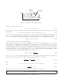
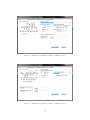
• To run iREG one has to double click the icon entitled iREG.exe. A window like the one in Fig.1.1 will
appear.
• Next you should select the proper button depending on what you want to do (identify a plant model,
design a controller (robust digital or continuous) or compute a reduced order controller).
• The program offers the possibility to switch between English and French interface.
1.3
Description of the software
After double clicking the program icon, 2 windows will be displayed: the main window (Figure 1.1) witch gives
access to all the functionality of the program and the plots window witch shows the graphics. Each window is
organized in tabs. The main window contains the following tabs:
• Start - starting tab of the application, the different functionalities of the program (identification, controller
design or controller reduction) can be activated from this tab; furthermore, it an be used to save/load the
workspace;
• Identification - this tab gives access to all identification routines implemented in iREG and can also be
used to modify the graphics associated with the identification part of this software;
3
Figure 1.1: Start window of the application
• Architecture - includes all necessary functionality represents the initial tab for designen a controller; one
can select the type of controller to be design (digital RST or continuous PI/PID), load the plant model,
save the controller or test an already computed controller;
• Controller Design - offers all necessary tools to design and properly adjust all parameters of a robust
digital controller;
• Automated controller Design - offers only the basic tools to design and adjust a robust digital controller;
• PI/PID - offers the possibility of implementing a continuous PI or PID controller;
• Analysis Plots - can be used to display graphics and modify their appearance;
• Band-stop Filters - used to implement filters for the precise shaping of the sensibility functions;
• Tracking - for designing the tracking part of a digital controller (reference model and polynomial T );
• Reduc - can be used to reduce the order of a RST controller;
• About iREG - information regarding the software (name, version, authors and copyright).
4
Part I
Identification
5
Chapter 2
Basic theory
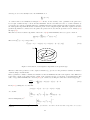
The recursive parameter estimation principle for sampled models is illustrated in Figure 2.1.
DI SCRETI ZED PL ANT
u(t)
y(t)
D.A.C.
+
PL ANT
A.D.C.
Z.O.H.
+
ε(t)
Adjustable
Discrete-time
Model
estimated
model
par ameter s
y(t)
Par ameter
Adaptation
Algor ithm
Figure 2.1: Parameter estimation principle
A discrete time model with adjustable parameters is implemented on the computer. The error between the
system output at instant t, y(t) and the output predicted by the model yˆ(t) (called plant-model error or
prediction error) is used by the parameter adaptation algorithm, which, at each sampling instant, will modify
the model parameters in order to minimize this error (in the sense of a certain criterion).
The input to the system is a low level and frequency rich signal generated by the computer, for the case of
plant model identification in open loop, or a combination of this and the signal generated by the controller in
the case of closed loop identification.
The key element for implementing the on-line estimation of the plant model parameters is the parameter
adaptation algorithm (PAA) which drives the parameters of the adjustable prediction model from the data
acquired on the system at each sampling instant. This algorithm has a recursive structure, i.e., the new value
of the estimated parameters is equal to the previous value plus a correcting term which will depend on the most
recent measurements.
In general a parameter vector is defined. Its components are the different parameters that should be estimated.
6
The parameter adaptation algorithms generally have the following structure:

 
 
N ew estimated
P revious estimated
Adaptation
 parameters  = 
+
parameters
gain
(vector)
(vector)
(matrix)

 
M easurement
P rediction error
×
f unction
f unction
×
(vector)
(scalar)




This structure corresponds to the so-called integral type adaptation algorithms (the algorithm has memory and
therefore maintains the estimated value of the parameters when the correcting terms become null). The algorithm can be viewed as a discrete-time integrator fed at each instant by the correcting term. The measurement
function vector is generally called the observation vector . The prediction error function is generally called the
adaptation error .
As will be shown, there are more general structures where the integrator is replaced by other types of dynamics,
i.e., the new value of the estimated parameters will be equal to a function of the previous parameter estimates
(eventually over a certain horizon) plus the correcting term.
The adaptation gain plays an important role in the performances of the parameter adaptation algorithm and it
may be constant or time-varying.
The problem addressed in this chapter is the synthesis and analysis of parameter adaptation algorithms in a
deterministic environment.
2.1
Gradient Algorithm
The aim of the gradient parameter adaptation algorithm is to minimize a quadratic criterion in terms of the
prediction error.
Consider the discrete-time model of a plant described by:
y(t + 1) = −a1 y(t) + b1 u(t) = θT φ(t)
(2.1)
where the unknown parameters a1 and b1 form the components of the parameter vector θ:
θT = [a1 , b1 ]
(2.2)
φT (t) = [−y(t), u(t)]
(2.3)
and
is the measurement vector .
The adjustable prediction model will be described in this case by:
ˆ
yˆ0 (t + 1) = yˆ[(t + 1)/θ(t)]
= −aˆ1 (t)y(t) + ˆb(t)u(t) = θˆT (t)φ(t)
(2.4)
where yˆ0 (t + 1) is termed the a priori predicted output depending on the value of the estimated parameter
vector at instant t,
θˆT (t) = [aˆ1 (t), bˆ1 (t)]
(2.5)
As it will be shown later, it is very useful to consider also the a posteriori predicted output computed on the
ˆ + 1), which will be available somewhere between t + 1
basis of the new estimated parameter vector at t + 1, θ(t
and t + 2. The a posteriori predicted output will be given by:
yˆ(t + 1)
ˆ + 1)]
yˆ[(t + 1)|θ(t
= −ˆ
a1 (t + 1)y(t) + ˆb1 (t + 1)u(t)
= θˆT (t + 1)φ(t)
=
(2.6)
One defines an a priori prediction error,
0 (t + 1) = y(t + 1) − yˆ0 (t + 1)
7
(2.7)
sense of
adaptation
b1
AAA
AAA
AAA
gradient
a1
Figure 2.2: Principle of the gradient method
and an a posteriori prediction error,
(t + 1) = y(t + 1) − yˆ(t + 1)
(2.8)
The objective is to find a recursive parameter adaptation algorithm with memory. The structure of such an
algorithm is:
ˆ + 1) = θ(t)
ˆ + ∆θ(t
ˆ + 1) = θ(t)
ˆ + f [θ(t),
ˆ φ(t), 0 (t + 1)]
θ(t
(2.9)
ˆ φ(t), 0 (t + 1)] must depend solely on the information available at the instant (t + 1)
The correction term f [θ(t),
ˆ
when y(t + 1) is acquired (last measurement y(t + 1), θ(t),
and a finite amount of information at times t, t − 1,
t − 2, · · · , t − n). The correction term must enable the following criterion to be minimized at each step:
min J(t + 1) = [0 (t + 1)]2
ˆ
θ(t)
(2.10)
A solution can be provided by the gradient technique.
If the iso-criterion curves (J = constant) are represented in the plane of the parameters a1 , b1 , concentric
closed curves are obtained around the minimum value of the criterion, which is reduced to the point (a1 , b1 )
corresponding to the parameters of the plant model. As the value of J = const. increases, the iso-criterion
curves move further and further away from the minimum. This is illustrated in Figure 2.2. In order to minimize
the value of the criterion, one moves in the opposite direction of the gradient to the corresponding iso-criterion
curve. This will lead to a curve corresponding to J = const, of a lesser value, as is shown in Figure 2.2. The
corresponding parametric adaptation algorithm will have the form:
ˆ + 1) = θ(t)
ˆ − F δJ(t + 1)
θ(t
ˆ
δ θ(t)
(2.11)
ˆ is the
where F = αI(α > 0) is the matrix adaptation gain (I - unitary diagonal matrix) and δJ(t + 1)/δ θ(t)
ˆ
gradient of the criterion given in (2.10) with respect to θ(t). From (2.10) one obtains:
1 δJ(t + 1)
δ0 (t + 1) 0
=
(t + 1)
ˆ
ˆ
2 δ θ(t)
δ θ(t)
(2.12)
0 (t + 1) = y(t + 1) − yˆ0 (t + 1) = y(t + 1) − θˆT (t)φ(t)
(2.13)
δ0 (t + 1)
= −φ(t)
ˆ
δ θ(t)
(2.14)
But:
and
Introducing (2.14) in (2.12), the parameter adaptation algorithm of (2.11) becomes:
ˆ + 1) = θ(t)
ˆ + F φ(t)0 (t + 1)
θ(t
where F is the matrix adaptation gain. There are two possible choices:
8
(2.15)
1. F = αI; α > 0
2. F > 0 (positive definite matrix)1
ˆ + 1) = θ(t)).
ˆ
The resulting algorithm has an integral structure. Therefore it has memory (for ε0 (t + 1) = 0, θ(t
The geometrical interpretation of the PAA of (2.15) is given in Figure 2.3.
The correction is done in the direction of the observation vector (which in this case is the measurement vector)
in the case F = αI, α > 0 or within ±90 deg around this direction when F > 0 (a positive definite matrix may
cause a rotation of a vector for less than 90 deg).
φ(t)
θ (t+1)
θ (t+1)
Fφ(t)ε (t+1) ; F = αI
Fφ(t)ε (t+1) ; F > 0
θ(t)
Figure 2.3: Geometrical interpretation of the gradient adaptation algorithm
The parameter adaptation algorithm given in (2.15) presents instability risks if a large adaptation gain (respectively a large α) is used. This can be understood by referring to Figure 2.2. If the adaptation gain is large near
the optimum, one can move away from this minimum instead of getting closer.
The following analysis will allow to establish necessary conditions upon the adaptation gain in order to avoid
instability.
Consider the parameter error defined as:
˜ = θ(t)
ˆ −θ
θ(t)
(2.16)
From Eqs. 2.1 and 2.4 it results:
˜
0 (t + 1) = y(t + 1) − yˆ0 (t + 1) = θT φ(t) − θˆT (t)φ(t) = −φT (t)θ(t)
(2.17)
Subtracting θ in the two terms of (2.15) and using (2.17) one gets:
˜ + 1)
θ(t
˜ − F (t)φ(t)φT (t)θ(t)
˜ = [I − F φ(t)φT (t)]θ(t)
˜
θ(t)
˜
= A(t)θ(t)
=
(2.18)
(2.18) corresponds to a time-varying dynamical system. A necessary stability condition (but not sufficient) is
that the eigen values of A(t) be inside the unit circle at each instant t. This leads to the following condition for
the choice of the adaptation gain as F = αI:
α<
2.1.1
1
φT (t)φ(t)
(2.19)
Improved Gradient Algorithm
In order to assure the stability of the PAA for any value of the adaptation gain α (or of the eigenvalues of the
gain matrix F ) the same gradient approach is used but a different criterion is considered:
min J(t + 1) = [(t + 1)]2
ˆ
θ(t+1)
(2.20)
1 A symmetric square matrix F is termed positive definite if xT F x > 0 for all x 6= 0, x ∈ <n . In addition: (i) all the terms of
the main diagonal are positive, (ii) the determinants of all the principals minors are positive.
9
The equation:
δ(t + 1)
1 δJ(t + 1)
=
(t + 1)
ˆ + 1)
ˆ + 1)
2 δ θ(t
δ θ(t
(2.21)
is then obtained. From (2.6) and (2.8) it results that:
(t + 1) = y(t + 1) − yˆ(t + 1) = y(t + 1) − θˆT (t + 1)φ(t)
(2.22)
δ(t + 1)
= −φ(t)
ˆ + 1)
δ θ(t
(2.23)
and, respectively:
Introducing (2.23) in (2.21), the parameter adaptation algorithm of (2.11) becomes:
ˆ + 1) = θ(t)
ˆ + F φ(t)(t + 1)
θ(t
(2.24)
ˆ + 1). For implementing this algorithm, ε(t + 1)
This algorithm depends on ε(t + 1), which is a function of θ(t
0
ˆ φ(t), ε0 (t + 1)]
must be expressed as a function of ε (t + 1), i.e. ε(t + 1) = f [θ(t),
(2.22) can be rewritten as:
ˆ + 1) − θ(t)]
ˆ T φ(t)
(t + 1) = y(t + 1) − θˆT (t)φ(t) − [(θ(t
(2.25)
The first two terms of the right hand side correspond to ε0 (t + 1), and from (2.24), one obtains:
ˆ + 1) − θ(t)
ˆ = F φ(t)(t + 1)
θ(t
(2.26)
(t + 1) = 0 (t + 1) − φT (t)F φ(t)(t + 1)
(2.27)
which enables to rewrite (2.25) as:
from which the desired relation between ε(t + 1) and ε0 (t + 1) is obtained:
(t + 1) =
0 (t + 1)
1 + φT (t)F φ(t)
(2.28)
and the algorithm of (2.24) becomes:
0
ˆ + 1) = θ(t)
ˆ + F φ(t) (t + 1)
θ(t
T
1 + φ (t)F φ(t)
(2.29)
which is a stable algorithm irrespective of the value of the gain matrix F (positive definite).
The division by 1 + φT (t)F φ(t) introduces a normalization with respect to F and φ(t) which reduces the
sensitivity of the algorithm with respect to F and φ(t).
ˆ is given by:
In this case, the equation for the evolution of the parametric error θ(t)
F φ(t)φT (t)
˜
˜ = A(t)θ˜T (t)
θ(t + 1) = I −
θ(t)
(2.30)
1 + φT (t)F φ(t)
and the eigenvalues of A(t) will always be inside or on the unit circle, but this is not enough to conclude upon
the stability of the algorithm.
2.2
Recursive Least Squares Algorithm
When using the Gradient Algorithm, 2 (t + 1) is minimized at each step or, to be more precise, one moves in
the quickest decreasing direction of the criterion, with a step depending on F . The minimization of 2 (t + 1) at
10
each step does not necessarily lead to the minimization of:
t
X
2 (i + 1)
i=1
on a time horizon, as is illustrated in Figure 2.4. In fact, in the vicinity of the optimum, if the gain is not
low enough, oscillations may occur around the minimum. On the other hand, in order to obtain a satisfactory
convergence speed at the beginning when the optimum is far away, a high adaptation gain is preferable. In fact,
the least squares algorithm offers such a variation profile for the adaptation gain. The same equations as in the
gradient algorithm are considered for the plant, the prediction model, and the prediction errors, namely (2.1)
through (2.8).
The aim is to find a recursive algorithm of the form of (2.9) which minimizes the least squares criterion:
min J(t) =
ˆ
θ(t)
t
X
[y(i) − θˆT (t)φ(i − 1)]2
(2.31)
i=1
ˆ T φ(i − 1) corresponds to:
The term θ(t)
ˆ
θˆT (t)φ(i − 1) = −ˆ
a1 (t)y(i − 1) + ˆb1 (t)u(i − 1) = yˆ[i | θ(t)]
(2.32)
b1
a1
Figure 2.4: Evolution of an adaptation algorithm of the gradient type
Therefore, this is the prediction of the output at instant i(i ≤ t) based on the parameter estimate at instant t
obtained using t measurements.
First, a parameter θ must be estimated at instant t so that it minimizes the sum of the squares of the differences
between the output of the plant and the output of the prediction model on a horizon of t measurements. The
ˆ
ˆ
value of θ(t),
which minimizes the criterion (2.31), is obtained by seeking the value that cancels δJ(t)/δ θ(t):
t
X
δJ(t)
[y(i) − θˆT (t)φ(i − 1)]φ(i − 1) = 0
= −2
ˆ
δ θ(t)
(2.33)
i=1
From (2.33), taking into account that:
ˆ
[θˆT (t)φ(i − 1)]φ(i − 1) = φ(i − 1)φT (i − 1)θ(t)
one obtains:
"
t
X
#
ˆ =
φ(i − 1)]φT (i − 1) θ(t)
i=1
t
X
y(i)φ(i − 1)
i=1
and left multiplying by2 :
"
t
X
#−1
T
φ(i − 1)φ (i − 1)
i=1
2 It
is assumed that the matrix
condition
Pt
i=1
φ(i − 1)φT (i − 1) is invertible. As it will be shown later this corresponds to an excitation
11
one obtains:
"
ˆ
θ(t)
=
t
X
#−1
T
φ(i − 1)φ (i − 1)
i=1
= F (t)
t
X
y(i)φ(i − 1)
i=1
t
X
y(i)φ(i − 1)
(2.34)
i=1
in which:
F (t)−1 =
t
X
φ(i − 1)φT (i − 1)
(2.35)
i=1
ˆ + 1)
This estimation algorithm is not recursive. In order to obtain a recursive algorithm, the estimation of θ(t
is considered:
ˆ + 1) = F (t + 1)
θ(t
t+1
X
y(i)φ(i − 1)
(2.36)
i=1
F (t + 1)−1 =
t+1
X
φ(i − 1)φT (i − 1) = F (t)−1 + φ(t)φT (t)
(2.37)
i=1
ˆ + 1) as a function of θ(t):
ˆ
We can now express θ(t
ˆ + 1) = θ(t)
ˆ + ∆θ(t
ˆ + 1)
θ(t
(2.38)
From (2.37) one has:
ˆ + 1) = F (t + 1)
θ(t
" t
X
#
y(i)φ(i − 1) + y(t + 1)φ(t)
(2.39)
i=1
Taking into account (2.34), (2.39) can be rewritten as:
ˆ + 1) = F (t + 1)[F (t)−1 θ(t)
ˆ + y(t + 1)φ(t)]
θ(t
(2.40)
ˆ one gets:
From (2.37) after post-multiplying both sides by θ(t)
ˆ = F (t + 1)−1 θ(t)
ˆ − φ(t)φT (t)θ(t)
ˆ
F (t)−1 θ(t)
(2.41)
n
o
ˆ + 1) = F (t + 1) F (t + 1)−1 θ(t)
ˆ + φ(t)[y(t + 1) − θˆT (t)φ(t)]
θ(t
(2.42)
and (2.40), becomes:
Taking into account the expression of 0 (t + 1) given by (2.13), the result is:
ˆ + 1) = θ(t)
ˆ + F (t + 1)φ(t)0 (t + 1)
θ(t
(2.43)
The adaptation algorithm of (2.43) has a recursive form similar to the gradient algorithm given in (2.15) except
that the gain matrix F (t + 1) is now time-varying since it depends on the measurements (it automatically
corrects the gradient direction and the step length). A recursive formula for F (t + 1) remains to be given from
the recursive formula F −1 (t + 1) given in (2.37). This is obtained by using the matrix inversion lemma.
Matrix Inversion Lemma: Let F be a (n × n) dimensional nonsingular matrix, R a (m × m) dimensional
nonsingular matrix and H a (n × m) dimensional matrix of maximum rank, then the following identity holds:
(F −1 + HR−1 H T )−1 = F − F H(R + H T F H)−1 H T F
12
(2.44)
Proof : By direct multiplication one finds that:
[F − F H(R + H T F H)−1 H T F ][F −1 + HR−1 H T ] = I
For the case of (2.37), one chooses H = φ(t), R = 1 and one obtains from (2.37) and (2.44):
F (t + 1) = F (t) −
F (t)φ(t)φT (t)F (t)
1 + φT (t)F (t)φ(t)
(2.45)
and, putting together the different equations, a first formulation of the recursive least squares (RLS) parameter
adaptation algorithm (PAA) is given below:
ˆ + 1) = θ(t)
ˆ + F (t + 1)φ(t)0 (t + 1)
θ(t
F (t)φ(t)φT (t)F (t)
F (t + 1) = F (t) −
1 + φT (t)F (t)φ(t)
0
(t + 1) = y(t + 1) − θˆT (t)φ(t)
(2.46)
(2.47)
(2.48)
An equivalent form of this algorithm is obtained by introducing the expression of F (t + 1) given by (2.47) in
(2.46), where:
ˆ + 1) − θ(t)]
ˆ
[θ(t
= F (t + 1)φ(t)0 (t + 1)
0 (t + 1)
= F (t)φ(t)
1 + φT (t)F (t)φ(t)
(2.49)
However, from (2.7), (2.8) and (2.49), one obtains:
(t + 1) = y(t + 1) − θˆT (t + 1)φ(t) =
ˆ + 1) − θ(t)]
ˆ T φ(t) =
−[θ(t
0 (t + 1)
=
−φT (t)F (t)φ(t)
1 + φT (t)F (t)φ(t)
ˆ
y(t + 1) − θ(t)φ(t)
0 (t + 1)
0 (t + 1)
1 + φT (t)F (t)φ(t)
(2.50)
which expresses the relation between the a posteriori prediction error and the a priori prediction error. Using
this relation in (2.49), an equivalent form of the parameter adaptation algorithm for the recursive least squares
is obtained:
ˆ + 1) = θ(t)
ˆ + F (t)φ(t)(t + 1)
θ(t
F (t + 1)−1 = F (t)−1 + φ(t)φT (t)
F (t)φ(t)φT (t)F (t)
F (t + 1) = F (t) −
1 + φT (t)F (t)φ(t)
y(t + 1) − θˆT (t)φ(t)
(t + 1) =
1 + φT (t)F (t)φ(t)
(2.51)
(2.52)
(2.53)
(2.54)
For the recursive least squares algorithm to be exactly equivalent to the non-recursive least squares algorithm,
it must be started from a first estimation obtained at instant t0 = dim φ(t), since normally F (t)−1 given by
(2.35) becomes nonsingular for t = t0 . In practice, the algorithm is started up at t = 0 by choosing:
F (0) =
1
I = (GI)I; 0 < δ 1
δ
(2.55)
a typical value being δ = 0.001(GI = 1000). It can be observed in the expression of F (t + 1)−1 given by (2.37)
that the influence of this initial error decreases with the time. In this case one minimizes the following criterion:
min J(t) =
ˆ
θ(t)
t
X
ˆ T
[y(i) − θˆT (t)φ(i − 1)]2 + [θ − θˆT (0)]T F (0)−1 [θ − θ(0)]
i=1
13
(2.56)
A rigorous analysis shows nevertheless that for any positive definite matrix F (0)[F (0) > 0],
lim (t + 1) = 0
t→∞
The recursive least squares algorithm is an algorithm with a decreasing adaptation gain. This is clearly seen if
the estimation of a single parameter is considered. In this case, F (t) and φ(t) are scalars, and (2.53) becomes:
F (t)
≤ F (t);
1 + φ(t)2 F (t)
F (t + 1) =
φ(t), F (t) ∈ R1
The same conclusion is obtained observing that F (t + 1)−1 is the output of an integrator which has as input
φ(t)φT (t). Since φ(t)φT (t) ≥ 0, one conclude that if φ(t)φT (t) > 0 in the average, then F (t)−1 will tends
towards infinity, i.e., F (t) will tends towards zero.
The recursive least squares algorithm in fact gives less and less weight to the new prediction errors and thus
to the new measurements. Consequently, this type of variation of the adaptation gain is not suitable for the
estimation of time-varying parameters, and other variation profiles for the adaptation gain must therefore be
considered. Under certain conditions the adaptation gain is a measure of the evolution of the covariance of the
parameter estimation error.
ˆ and φ(t) of dimension 2 may be generalized for any
The least squares algorithm presented up to now for θ(t)
dimensions resulting from the description of discrete-time systems of the form:
y(t) =
q −d B(q −1 )
u(t)
A(q −1 )
(2.57)
where:
A(q −1 )
B(q
−1
=
)
1 + a1 q −1 + · · · + anA q −nA
= b1 q
−1
+ · · · + bn B q
−nB
(2.58)
(2.59)
(2.57) can be written in the form:
y(t + 1) = −
nA
X
ai y(t + 1 − i) +
i=1
nB
X
bi u(t − d − i + 1) = θT φ(t)
(2.60)
i=1
in which:
θT
=
[a1 , · · · , anA , b1 , · · · , bnB ]
φ (t)
=
[−y(t) · · · − y(t − nA + 1), u(t − d)
T
· · · u(t − d − nB + 1)]
(2.61)
(2.62)
The a priori adjustable predictor is given in the general case by:
yˆ0 (t + 1)
=
−
nA
X
a
ˆi (t)y(t + 1 − i) +
i=1
nB
X
ˆb1 (t)u(t − d − i + 1)
i=1
= θˆT (t)φ(t)
(2.63)
in which:
θˆT (t) = [ˆ
a1 (t), · · · , a
ˆnA (t), ˆb1 (t), · · · , ˆbnB (t)]
(2.64)
ˆ
and for the estimation of θ(t), the algorithm given in (2.51) through (2.54) is used, with the appropriate
ˆ
dimension for θ(t),
φ(t) and F (t).
2.3
Choice of the Adaptation Gain
The recursive formula for the inverse of the adaptation gain F (t + 1)−1 given by (2.52) is generalized by
introducing two weighting sequences λ1 (t) and λ2 (t), as indicated below:
F (t + 1)−1 = λ1 (t)F (t)−1 + λ2 (t)φ(t)φT (t)
0 < λ1 (t) ≤ 1 ; 0 ≤ λ2 (t) < 2 ; F (0) > 0
14
(2.65)
Note that λ1 (t) and λ2 (t) in (2.65) have the opposite effect. λ1 (t) < 1 tends to increase the adaptation gain (the
gain inverse decreases); λ2 (t) > 0 tends to decrease the adaptation gain (the gain inverse increases). For the
purpose of this manual only the influence of λ1 will be discussed as it is the chosen parameter for implementing
different adaptation schemes.
Using the matrix inversion lemma given by (2.44), one obtains from (2.65):


T
F (t)φ(t)φ (t)F (t) 
1 
F (t) − λ (t)
(2.66)
F (t + 1) =
1
λ1 (t)
+ φT (t)F (t)φ(t)
λ2 (t)
Next, a certain number of choices for λ1 (t) and their interpretations will be given.
A.1: Decreasing (vanishing) gain (RLS). In this case:
λ1 (t) = λ1 = 1; λ2 (t) = 1
(2.67)
and F (t + 1)−1 is given by (2.52), which leads to a decreasing adaptation gain. The minimized criterion is that
of (2.31). This type of profile is suited to the estimation of the parameters of stationary systems.
A.2: Constant forgetting factor . In this case:
λ1 (t) = λ1 ; 0 < λ1 < 1; λ2 (t) = λ2 = 1
(2.68)
The typical values for λ1 are:
λ1 = 0.95 to 0.99
The criterion to be minimized will be:
J(t) =
t
X
(t−i)
λ1
[y(i) − θˆT (t)φ(i − 1)]2
(2.69)
i=1
The effect of λ1 (t) < 1 is to introduce increasingly weaker weighting on the old data (i < t). This is why λ1
is known as the forgetting factor. The maximum weight is given to the most recent error. This type of profile
is suited to the estimation of the parameters of slowly time-varying systems. The use of a constant forgetting
factor without the monitoring of the maximum value of F (t) causes problems in adaptive regulation if the
{φ(t)φT (t)} sequence becomes null in the average (steady state case) because the adaptation gain will tend
towards infinity. In this case:
F (t + i)−1 = (λ1 )i F (t)−1
and:
F (t + i) = (λ1 )−i F (t)
For: λ1 < 1, lim (λ1 )−i = ∞ and F (t + i) will become asymptotically unbounded.
i→∞
A.3: Variable forgetting factor . In this case:
λ2 (t) = λ2 = 1
(2.70)
λ1 (t) = λ0 λ1 (t − 1) + 1 − λ0 ; 0 < λ0 < 1
(2.71)
and the forgetting factor λ1 (t) is given by:
The typical values being:
λ1 (0) = 0.95 to 0.99 ; λ0 = 0.5 to 0.99
(λ1 (t) can be interpreted as the output of a first order filter (1 − λ0 )/(1 − λ0 q −1 ) with a unitary steady state
gain and an initial condition λ1 (o)).
Relation (2.71) leads to a forgetting factor that asymptotically tends towards 1. The criterion minimized will
be:


t
t
Y
X

J(t) =
λ1 (j − i) [y(i) − θˆT (t)φ(i − 1)]2
(2.72)
i=1
j=1
15
As λ1 tends towards 1 for large i, only the initial data are forgotten (the adaptation gain tends towards a
decreasing gain).
This type of profile is highly recommended for the model identification of stationary systems, since it avoids
a too rapid decrease of the adaptation gain, thus generally resulting in an acceleration of the convergence (by
maintaining a high gain at the beginning when the estimates are at a great distance from the optimum).
Other types of evolution for λ1 (t) can be considered. For example:
λ1 (t) = 1 −
φT (t)F (t)φ(t)
1 + φT (t)F (t)φ(t)
This forgetting factor depends upon the input/output signals via φ(t). It automatically takes the value 1 if the
norm of φ(t)φT (t) becomes null. In the cases where the φ(t) sequence is such that the term φT (t)F (t)φ(t) is
significative with respect to one, the forgetting factor takes a lower value assuring good adaptation capabilities
(this is related to the concept of ”persistently exciting” signal).
Another possible choice is:
[0 (t)]2
λ1 (t) = 1 − α
; α>0
1 + φT (t)F (t)φ(t)
The forgetting factor tends towards 1, when the prediction error tends towards zero. Conversely, when a change
occurs in the system parameters, the prediction error increases leading to a forgetting factor less than 1 in order
to assure a good adaptation capability.
Choice of the initial gain F (0).
The initial gain F (0) is usually chosen as a diagonal matrix of the form given by (2.55) and, respectively,


GI
0


..
F (0) = 
(2.73)

.
0
GI
In the absence of initial information upon the parameters to be estimated (typical value of initial estimates
= 0), a high initial gain (GI) is chosen. A typical value is GI = 1000 (but higher values can be chosen).
If an initial parameter estimation is available (resulting for example from a previous identification), a low initial
gain is chosen. In general, in this case GI ≤ 1.
Since in standard RLS the adaptation gain decreases as the true model parameters are approached (a significant
measurement is its trace), the adaptation gain may be interpreted as a measurement of the accuracy of the
parameter estimation (or prediction). This explains the choices of F (0) proposed above. Note that under certain
hypotheses, F (t) is effectively a measurement of the quality of the estimation.
This property can give indications upon the evolution of a parameter estimation procedure. If the trace of
F (t) did not decrease significantly, the parameter estimation is in general poor. This may occur in system
identification when the level and type of input used are not appropriate.
2.4
Some Remarks on the Parameter Adaptation Algorithms
The parameter adaptation algorithms (PAA) presented up to now (integral type) have the form (λ1 = 1; λ2 = 1):
0
ˆ + 1) = θ(t)
ˆ + F (t + 1)φ(t)0 (t + 1) = θ(t)
ˆ + F (t)φ(t) (t + 1)
θ(t
T
1 + φ (t)F (t)φ(t)
ˆ is the vector of estimated parameters and F (t + 1)φ(t)0 (t + 1) represents the correcting term at
where θ(t)
each sample.
F (t) is the adaptation gain (constant or time-varying), φ(t) is the observation vector and 0 (t + 1) is the a priori
prediction error (or in general the adaptation error), i.e., the difference between the measured output at the
ˆ
instant t + 1 and the predicted output at t + 1 based on the knowledge of θ(t).
16
There is always a relationship between the a priori prediction (adaptation) error 0 (t + 1) and the a posteriori
ˆ + 1). This relation is:
prediction (adaptation) error (t + 1) defined on the basis of the knowledge of θ(t
(t + 1) =
0 (t + 1)
1 + φT (t)F (t)φ(t)
Several types of updating formulas for the adaptation gain can be used in connection with the type of the
parameter estimation problem to be solved (systems with fixed or time-varying parameters), with or without
availability of initial information for the parameter to be estimated.
The PAA examined up to now are based on:
• minimization of a one step ahead criterion
• off-line minimization of a criterion over a finite horizon followed by a sequential minimization
• sequential minimization of a criterion over a finite horizon starting at t = 0
• relationship with the Kalman predictor.
However, from the point of view of real-time identification and adaptive control, the parameter adaptation
algorithms are supposed to operate on a very large number of measurements (t =⇒ ∞). Therefore, it is
necessary to examine the properties of parameter adaptation algorithms as t =⇒ ∞. Specifically, one should
study the conditions which guarantee:
lim (t + 1) = 0
t→∞
This corresponds to the study of the stability of parameter adaptation algorithms. Conversely, other parameter
adaptation algorithms will be derived from the stability condition given above.
2.5
Practical aspects of recursive open loop identification
In this section, the algorithms available in iREG for open loop plant model recusrive identification will be
presented. From a practical point of view, plant model identification is a key starting point for designing a high
perfomance linear controller.
Identification of dynamic systems is an experimental approach for determining a dynamic model of a system.
It includes four steps:
1. Input-output data acquisition under an experimental protocol.
2. Selection (or estimation) of the model complexity (structure).
3. Estimation of the model parameters.
4. Validation of the identified model (structure of the model and values of the parameters).
As it will be seen, the algorithms which will be used for parameter estimation will depend on the assumptions
made on the noise disturbing the measurements, assumptions which have to be confirmed by the model validation
([6], [4], [5]). It is important to emphasize that no one single plant + disturbance structure exists that can
describe all the situations encountered in practice. Furthermore, there is no parameter estimation algorithms
that may be used with all possible plant + disturbance structures such that the estimated parameters are always
unbiased. Furthermore, due to the lack of a priori information, the input-output data acquisition protocol may
be initially inappropriate.
All these causes may lead to identified models which do not pass the validation test, and therefore the identification should be viewed as an iterative process as illustrated in Figure 2.5.
17
I/0 Data Acquisition
under an Experimental Protocol
Model Complexity Estimation
(or Selection)
Choice of the Noise Model
Parameter Estimation
Model Validation
No
Yes
Control
Design
Figure 2.5: The iterative process of identification
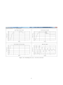
Tables 2.1-2.3 summarizes a number of significant recursive parameter estimation techniques. They all use PAA
of the form:
ˆ + 1)
θ(t
F (t + 1)
−1
ˆ + F (t)Φ(t)ν(t + 1)
θ(t)
(2.74)
= λ1 (t)F (t) + λ2 (t)Φ(t)ΦT (t)
(2.75)
=
0 < λ1 (t) ≤ 1
F
2.5.1
−1
;
0 ≤ λ2 (t) < 2; F (0) > 0
(0)
;
ν(t + 1)
=
0<α<∞
ν 0 (t + 1)
1 + ΦT (t)F (t)Φ(t)
(t) > αF
−1
(2.76)
Validation of the Models Identified with Type I Methods
This section is concerned with the validation of models identified using identification methods based on the
whitening of the prediction error.
If the residual prediction error is a white noise sequence, in addition to obtaining unbiased parameter estimates,
this also means that the identified model gives the best prediction for the plant output in the sense that it
minimizes the variance of the prediction error. On the other hand, since the residual error is white and a white
noise is not correlated with any other variable, then all the correlations between the input and the output of
the plant are represented by the identified model and what remains unmodelled does not depend on the input.
The principle of the validation method is as follows:
• If the plant + disturbance structure chosen is correct, i.e., representative of reality.
• If an appropriate identification method for the structure chosen has been used.
• If the degrees of the polynomials A(q −1 ), B(q −1 ), C(q −1 ) and the value of d (delay) have been correctly
chosen (the plant model is in the model set).
Then the prediction error (t) asymptotically tends toward a white noise, which implies:
lim E{(t)(t − i)} = 0;
t→∞
i = 1, 2, 3 · · · ; −1, −2, −3 · · ·
The validation method implements this principle. It is made up of several steps:
1 - Creation of an I/O file for the identified model (using the same input sequence as for the system).
2 - Creation of a prediction error file for the identified model (minimum 100 data).
3 - Whiteness (uncorrelatedness) test on the prediction errors sequence (also known as residual prediction
errors).
18
19
Predictor
a priori
Output
a posteriori
Prediction a priori
Error
a posteriori
Adaptation Error
Observation Vector
Predictor Regressor
Vector
Plant + Noise Model
Adjustable Parameter
Vector
φT (t) = [−y(t) . . . − y(t − nA + 1),
u(t − d) . . . u(t − d − nB + 1)]
y = q A B u + A1 e
T
ˆ
θ (t) = [ˆ
aT (t), ˆbT (t)]
T
a
ˆ (t) = [ˆ
a1 . . . a
ˆnA ]
ˆbT (t) = [ˆb1 . . . ˆbn ]
B
−d
yˆ0 (t + 1) = θˆT (t)φ(t)
yˆ(t + 1) = θˆT (t + 1)φ(t)
0 (t + 1) = y(t + 1) − yˆ0 (t + 1)
(t + 1) = y(t + 1) − yˆ(t + 1)
ν ◦ (t + 1) = ◦ (t + 1)
Φ(t) = φ(t)
φT (t) = [−y(t) . . . − y(t − nA + 1),
u(t − d) . . . u(t − d − nB + 1),
(t) . . . (t − nC + 1)]
−d
y = q AB u + C
Ae
T
ˆ
θ (t) = [ˆ
aT (t), ˆbT (t), cˆT (t)]
a
ˆT (t) = [ˆ
a1 . . . a
ˆnA ]
ˆbT (t) = [ˆb1 . . . ˆbn ]
B
cˆT (t) = [ˆ
c1 . . . cˆnC ]
Table 2.1: Recursive identification algorithms
Recursive
Extended
Least Squares (RLS)
Least Squares (RELS)
−d
y = q AB u + C
Ae
T
ˆ T (t)]
ˆ (t) = [ˆ
Θ
aT (t), ˆbT (t), h
T
a
ˆ (t) = [ˆ
a1 . . . a
ˆnA ]
ˆbT (t) = [ˆb1 . . . ˆbn ]
B
ˆ T (t) = [h
ˆ1 . . . h
ˆn ]
h
H
nH = max(nA , nC )
φT (t) = [−ˆ
y (t) . . . − yˆ(t − nA + 1),
u(t − d) . . . u(t − d − nB + 1),
(t) . . . (t − nC + 1)]
Output Error with Extended
Prediction Model (XOLOE)
20
Predictor
a priori
Output
a posteriori
Prediction a priori
Error
a posteriori
Adaptation Error
Observation Vector
Predictor Regressor
Vector
Plant + Noise Model
Adjustable Parameter
Vector
ˆ q −1 ) =
C(t,
Φ(t) =
1
φ(t)
−1 )
ˆ
C(t,q
1 + cˆ1 (t)q −1 +
...
φT (t) = [−y(t) . . . − y(t − nA + 1),
u(t − d) . . . u(t − d − nB + 1),
(t) . . . (t − nC + 1)]
y = q AB u + C
Ae
T
ˆ
θ (t) = [ˆ
aT (t), ˆbT (t), cˆT (t)]
a1 . . . a
ˆnA ]
a
ˆT (t) = [ˆ
ˆbT (t) = [ˆb1 . . . ˆbn ]
B
cˆT (t) = [ˆ
c1 . . . cˆnC ]
−d
−d
C
y = q A B u + AD
e
T
T
T
ˆ
ˆ
θ (t) = [ˆ
a (t), b (t), cˆT (t), dˆT (t)]
a1 . . . a
ˆ nA ]
a
ˆT (t) = [ˆ
ˆbT (t) = [ˆb1 . . . ˆbn ]
B
cˆT (t) = [ˆ
c1 . . . cˆnC ]
dˆT (t) = [dˆ1 . . . dˆnD ]
T
φ (t) = [−y(t) . . . − y(t − nA + 1),
u(t − d) . . . u(t − d − nB + 1),
(t) . . . (t − nC + 1),
−α(t) . . . − α(t − nD + 1)]
ˆ
ˆ ∗ (t)u(t − d − 1)
α(t) = A(t)y(t)
−B
0
yˆ (t + 1) = θˆT (t)φ(t)
yˆ(t + 1) = θˆT (t + 1)φ(t)
0
(t + 1) = y(t + 1) − yˆ0 (t + 1)
(t + 1) = y(t + 1) − yˆ(t + 1)
ν ◦ (t + 1) = ◦ (t + 1)
Φ(t) = φ(t)
Table 2.2: Recursive identification algorithms
Recursive Maximum
Generalized Least
Likelihood (RML)
Squares (GLS)
Φ(t) = φ(t)
φT (t) = [−ˆ
y (t) . . . − yˆ(t − nA + 1),
u(t − d) . . . u(t − d − nB + 1)]
−d
y = q AB u + v
T
ˆ
θ (t) = [ˆ
aT (t), ˆbT (t)]
T
a1 . . . a
ˆ nA ]
a
ˆ (t) = [ˆ
ˆbT (t) = [ˆb1 . . . ˆbn ]
B
Output Error
(OE)
21
Predictor
a priori
Output
a posteriori
Prediction a priori
Error
a posteriori
Adaptation Error
Observation Vector
Predictor Regressor
Vector
Plant + Noise Model
Adjustable Parameter
Vector
ˆ q −1 ) = 1 + a
A(t,
ˆ1 (t)q −1 + . . .
yIV (t) = θˆT (t)Φ(t − 1)
u(t − d) . . . u(t − nB − d + 1)]
yˆ0 (t + 1) = θˆT (t)φ(t)
yˆ(t + 1) = θˆT (t + 1)φ(t)
0 (t + 1) = y(t + 1) − yˆ0 (t + 1)
(t + 1) = y(t + 1) − yˆ(t + 1)
ν ◦ (t + 1) = ◦ (t + 1)
T
Φ (t) = [−yIV (t) . . . − yIV (t − nA + 1)
yˆ0 (t + 1) = θˆT (t)φ(t)
yˆ(t + 1) = θˆT (t + 1)φ(t)
ν ◦ (t + 1) = ◦ (t + 1)
Φ(t) = L(q1−1 ) φ(t)
1
Φ(t) = A(t,q
φ(t)
−1 )
ˆ
φT (t) = [−y(t) . . . − y(t − nA + 1),
u(t − d) . . . u(t − d − nB + 1)]
φT (t) = [−ˆ
y (t) . . . − yˆ(t − nA + 1),
u(t − d) . . . u(t − d − nB + 1)]
−d
y = q AB u + v
T
θˆ (t) = [ˆ
aT (t), ˆbT (t)]
T
a
ˆ (t) = [ˆ
a1 . . . a
ˆ nA ]
ˆbT (t) = [ˆb1 . . . ˆbn ]
B
y = q AB u + v
T
θˆ (t) = [ˆ
aT (t), ˆbT (t)]
T
a
ˆ (t) = [ˆ
a1 . . . a
ˆnA ]
ˆbT (t) = [ˆb1 . . . ˆbn ]
B
−d
Table 2.3: Recursive identification algorithms
Output Error with
Instrumental Variable with
(Adaptive) Filtered
Auxiliary Model (VI MAUX)
Observations (A)FOLOE
Φ(t) = φ(t)
ν ◦ (t + 1) = ◦ (t + 1)
−d
C
y = q AB u + D
e
T
T
T
θˆ (t) = [ˆ
a (t), ˆb (t), cˆT (t), dˆT (t)]
a
ˆT (t) = [ˆ
a1 . . . a
ˆ nA ]
ˆbT (t) = [ˆb1 . . . ˆbn ]
B
cˆT (t) = [ˆ
c1 . . . cˆnC ]
dˆT (t) = [dˆ1 . . . dˆnD ]
T
φ (t) = [−ˆ
x(t) . . . − x
ˆ(t − nA + 1),
u(t − d) . . . u(t − d − nB + 1)
vˆ(t) . . . vˆ(t − nB + 1)
−w(t)
ˆ . . . − w(t
ˆ − nB + 1)]
x
ˆ(t) = θ[1 : nA + nB ]T (t)φ[1 : nA + nB ](t)
vˆ(t) = y(t) − yˆ(t)
w(t)
ˆ = y(t) − x
ˆ(t)
yˆ0 (t + 1) = θˆT (t)φ(t)
yˆ(t + 1) = θˆT (t + 1)φ(t)
Box Jenkins
(BJ)
Table 2.4: Confidence intervals for whiteness tests
Level of
significance
Validation
criterion
N = 128
N = 256
N = 512
3%
2.17
√
N
0.192
0.136
0.096
5%
1.96
√
N
0.173
0.122
0.087
7%
1.808
√
N
0.16
0.113
0.08
Whiteness test
Let {(t)} be the centered sequence of the residual prediction errors (centered: measured value - mean value).
One computes:
R(0)
=
N
1 X 2
R(0)
(t) ; RN (0) =
=1
N t=1
R(0)
R(i)
=
N
R(i)
1 X
(t)(t − i) ; RN (i) =
N t=1
R(0)
i
=
1, 2, 3 · · · nA · · ·
(2.77)
(2.78)
with imax ≥ nA [degree of polynomial A(q −1 )], which are estimations of the (normalized) autocorrelations.
If the residual prediction error sequence is perfectly white (theoretical situation), and the number of samples is
very large (N → ∞), then RN (0) = 1; RN (i) = 0, i ≥ 13 .
In real situations, however, this is never the case (i.e., RN 6= 0; i ≥ 1), therefore, one considers as a practical
validation criterion (extensively tested on applications):
2.17
RN (0) = 1 ; | RN (i) |≤ √ ; i ≥ 1
N
(2.79)
where N is the number of samples.
This confidence interval corresponds to a 3% level of significance of the hypothesis test for Gaussian distribution.
Sharper confidence intervals can be defined. Table 2.4 gives the values of the validation criterion for various N
and various levels of significance.
The following remarks are important:
• An acceptable identified model has in general:
1.8
2.17
| RN (i) |≤ √ · · · √ ; i ≥ 1
N
N
• If several identified models have the same complexity (number of parameters), one chooses the model
given by the methods that lead to the smallest | RN (i) |.
• A too good validation criterion indicates that model simplifications may be possible.
• For simplicity’s sake, one can consider as a basic practical numerical value for the validation criterion
value:
| RN (i) |≤ 0.15 ; i ≥ 1
• If the level of the residual prediction errors is very low compared to the output level (let us say more than
60 dB), the whiteness tests lose their signification.
3 Conversely, for Gaussian data, uncorrelation implies independence. In this case, RN (i) = 0, i ≥ 1 implies independence
between (t), (t − 1) · · · , i.e., the sequence of residuals {(t)} is a Gaussian white noise.
22
2.5.2
Validation of the Models Identified with Type II Methods
This section is concerned with the validation of models obtained using the identification methods based on the
decorrelation between the observations and the prediction errors. The uncorrelation between the observations
and the prediction error leads to an unbiased parameter estimation. However, since the observations include the
predicted output which depends on the input, the uncorrelation between the residual prediction error and the
observations implies also that the residual prediction error is uncorrelated with the input. The interpretation
of this fact is that the residual prediction error does not contain any information depending upon the input,
i.e., all the correlations between the input and the output of the plant are represented by the identified model.
The principle of the validation method is as follows:
• If the disturbance is independent of the input (=⇒ E{w(t)u(t)} = 0).
• If the model + disturbance structure chosen is correct, i.e., representative of the reality.
• If an appropriate identification method has been used for the chosen structure.
• If the degrees of the polynomials A(q −1 ), B(q −1 ) and the value of d (delay) have been correctly chosen
(the plant model is in the model set).
then the predicted outputs yˆ(t − 1), yˆ(t − 2) · · · generated by a model of the form (output error type predictor):
ˆ −1 )ˆ
ˆ −1 )u(t)
A(q
y (t) = q −d B(q
(2.80)
and the prediction error (t) are asymptotically uncorrelated, which implies:
E {(t)ˆ
y (t − i)} ≈
N
1 X
(t)ˆ
y (t − i) = 0
N t=1
i = 1, 2, 3
The validation method implements this principle. It is made up of several steps:
1. Creation of an I/O file for the identified model (using the same input sequence as for the system).
2. Creation of files for the sequences {y(t)}; {ˆ
y (t)}; {(t)} (system output, model output, residual output
prediction error). These files must contain at least 100 data in order that the test be significant.
3. Uncorrelation test between the residual output prediction error sequence and the delayed prediction model
output sequences.
Uncorrelation test
Let {y(t)} and {ˆ
y (t)} be the centered output sequences of the plant and of the identified model, respectively.
Let {(t)} be the centered sequence of the residual output (prediction) errors (centered = measured values mean values). One computes:
R(i)
=
RN (i)
=
i
=
N
1 X
(t)ˆ
y (t − i) ; i = 0, 1, 2, · · · , nA · · ·
N t=1
h
1
N
PN
ˆ2 (t)
t=1 y
R(i)
P
1
N
N
2
t=1 (t)
0, 1, 2, · · · , nA · · ·
(2.81)
i1/2
(2.82)
which are estimations of the (normalized) cross-correlations (note that RN (0) 6= 1), and nA is the degree of
polynomial A(q −1 ).
If (t) and yˆ(t − i), i ≥ 1 are perfectly uncorrelated (theoretical situation), then:
RN (i) = 0 ; i = 1, 2, · · · , nA · · ·
23
In practice, one considers as a practical validation criterion:
2.17
| RN (i) |≤ √ ; i ≥ 1
N
where N is the number of samples. Table 2.4 can be used to find the numerical value of the validation criterion
for various N and the level of signification of the test.
All the comments made in the previous section apply also in this case. In particular, the basic practical numerical
value for the validation criterion, which is:
| RN (i) |< 0.15 ; i ≥ 1
is worth remembering.
This test is also used when one would like to compare models identified with Type I method, with models
identified with Type II method.
2.5.3
Selection of the Pseudo Random Binary Sequence
The correct parameter estimation requires the use of a rich signal (persistently exciting signal). Pseudo-random
binary sequences (PRBS) offer on the one hand a signal with a large frequency spectrum approaching the white
noise and, on the other hand, they have a constant magnitude. This allows to define precisely the level of the
instantaneous stress on the process (or actuator).
PRBS are sequences of rectangular pulses, modulated in width, that approximate a discrete-time white noise
and thus have a spectral content rich in frequencies. They owe their name pseudo random to the fact that they
are characterized by a sequence length within which the variations in pulse width vary randomly, but that over
a large time horizon, they are periodic, the period being defined by the length of the sequence. In the practice
of system identification, one generally uses just one complete sequence.
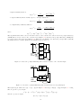
The PRBS are generated by means of shift registers with feedback (implemented in hardware or software). The
maximum length of a sequence is 2N − 1, in which N is the number of cells of the shift register. Figure 2.6
B1
B2
B4
B3
B5
+
( summation modulo 2 )
Figure 2.6: Generation of a PRBS of length 25 − 1 = 31 sampling periods
presents the generation of a PRBS of length 31 = 25 − 1 obtained by means of a 5-cells shift register.
Note that at least one of the N cells of the shift register should have an initial logic value different from zero
(one generally takes all the initial values of the N cells equal to the logic value 1).
Table 2.5 gives the structure enabling maximum length PRBS to be generated for different numbers of cells.
Note also a very important characteristic element of the PRBS: the maximum duration of a PRBS impulse is
equal to N (number of cells).
This property is to be considered when choosing a PRBS for system identification.
In order to correctly identify the steady-state gain of the plant dynamic model, the duration of at least one of
the pulses (e.g., the maximum duration pulse) must be greater than the rise time tR of the plant. The maximum
duration of a pulse being N.Ts , the following condition results:
N.Ts > tR
(2.83)
which is illustrated in Figure 2.8. From condition (2.83), one determines N and therefore the length of the
sequence, which is 2N − 1.
Furthermore, in order to cover the entire frequency spectrum generated by a particular PRBS, the length of a
test must be at least equal to the length of the sequence. In a large number of cases, the duration of the test
L is chosen equal to the length of the sequence. If the duration of the test is specified, it must therefore be
ensured that:
(2N − 1).Ts < L (L = test duration)
(2.84)
24
Table 2.5: Generation of maximum length PRBS
Number of Cells
N
2
3
4
5
6
7
8
9
10
Sequence Length
L = 2N − 1
3
7
15
31
63
127
255
511
1023
Bits Added
Bi and Bj
1 and 2
1 and 3
3 and 4
3 and 5
5 and 6
4 and 7
2,3,4 and 8
5 and 9
7 and 10
NTs > tR
tR
-----
NTs
Figure 2.7: Choice of a maximum duration of a pulse in a PRBS
Note that the condition (2.83) can result in fairly large values of N corresponding to sequence lengths of
prohibitive duration, either because Ts is very large, or because the system to be identified may well evolve
during the duration of the test. This is why, in a large number of practical situations, a submultiple of the
sampling frequency is chosen as the clock frequency for the PRBS. If:
fP RBS =
fs
; p = 1, 2, 3 · · ·
p
(2.85)
then condition 2.83 becomes:
p.N.Ts > tR
(2.86)
This approach is more interesting than the increase of the sequence length by increasing N in order to satisfy
(2.83).
Note that dividing the clock frequency of the PRBS will reduce the frequency range corresponding to a constant
spectral density in the high frequencies while augmenting the spectral density in the low frequencies. In general,
this will not affect the quality of identification, either because in many cases when this solution is considered,
the plant to be identified has a low band pass or because the effect or the reduction of the signal/noise ratio
at high frequencies can be compensated by the use of appropriate identification techniques. However, it is
recommended to choose p ≤ 4.
Figure 2.8 shows the spectral density of PRBS sequences generated with N = 8 for p = 1, 2, 3. As one can
see, the energy of the spectrum is reduced in the high frequencies and augmented in the lower frequencies.
Furthermore, for p = 3 a whole occurs at fs /3.
Up to now, we have been concerned only with the choice of the length and clock frequency of the PRBS;
however, the magnitude of the PRBS must also be considered. Although the magnitude of the PRBS may be
very low, it should lead to output variations larger than the residual noise level. If the signal/noise ratio is too
low, the length of the test must be augmented in order to obtain a satisfactory parameter estimation.
Note that in a large number of applications, the significant increase in the PRBS level may be undesirable in
view of the nonlinear character of the plants to be identified (we are concerned with the identification of a linear
model around an operating point).
2.5.4
Model Order Selection
In the absence of a clear a priori information upon the plant model structure, two approaches can be used to
select the appropriate orders for the values of d, nA , nB characterizing the input-output plant model.
25
Mag. [dB]
a) p = 1
20
10
0
−10
0
1
2
3
4
5
6
7
8
9
10
6
7
8
9
10
5
6
Frequency [Hz]
7
8
9
10
Mag. [dB]
b) p = 2
20
10
0
−10
0
1
2
3
4
5
Mag. [dB]
c) p = 3
20
10
0
−10
0
1
2
3
4
Figure 2.8: Spectral density of a PRBS sequence (fs = 20 Hz), a) N=8, p=1, b) N=8, p=2, c) N=8, p=3
a) a practical approach based on trial and error
b) estimation of d, nA , nB directly from data.
Even in the case of using an estimation of the orders directly from data it is useful to see to what extend the
two approaches are coherent.
We will discuss the two approaches next.
2.5.5
A Practical Approach for Model Order Selection
The plant + disturbance model to be identified is of the form:
A(q −1 )y(t) = q −d B(q −1 )u(t) + w(t)
where, according to the structures chosen, one has:
w(t)
= e(t)
w(t)
= A(q −1 )v(t); (v(t) and u(t) are independent)
= C(q −1 )e(t)
C(q −1 )
w(t) =
e(t)
D(q −1 )
w(t)
The degrees of the polynomials, A(q −1 ), B(q −1 ), C(q −1 ) and D(q −1 ) are respectively nA , nB , nC and nD . In
order to start the parameter estimation methods nA , nB and d must be specified. For the methods which
estimate also the noise model, one needs in addition to specify nC and nD .
A priori choice of nA Two cases can be distinguished:
1. Industrial plant (temperature, control, flow rate, concentration, and so on). For this type of plant in general:
nA ≤ 3
and the value nA = 2, which is very typical, is a good starting value to choose.
2. Electromechanical systems. nA results from the structural analysis of the system.
Example: Flexible Robot Arm with two vibration modes
In this case, nA = 4 is chosen, since a second-order is required, to model a vibratory mode.
Initial choice of d and nB If no knowledge of the time delay is available, d = 0 is chosen as an initial value.
If a minimum value is known, an initial value d = dmin is chosen.
If the time delay has been underestimated, during identification the first coefficients of B(q −1 ) will be very low.
nB must then be chosen so that it can both indicate the presence of the time delays and identify the transfer
function numerator. nB = (dmax − dmin ) + 2 is then chosen as the initial value.
At least two coefficients are required in B(q −1 ) because of the fractional delay which is often present in applications. If the time delay is known, nB ≥ 2 is chosen, but 2 remains a good initial value.
26
Determination of time delay d (first approximation) One identifies using the RLS (Recursive Least
Squares). The estimated numerator will be of the form:
ˆ −1 ) = ˆb1 q −1 + ˆb2 q −2 + ˆb3 q −3 + · · ·
B(q
If:
| ˆb1 |< 0.15 | ˆb2 |
b1 ≈ 0 is considered and time delay d is increased by 1 : d = dmin + 1 [since if b1 = 0, B(q −1 ) = q −1 (b2 q −1 +
b3 q −2 )]. If:
| ˆbi |< 0.15 | ˆbdi+1 | ; i = 1, 2, · · · , di
time delay d is increased by di : d = din + di . After these modifications, identification is restarted.
Determination of the (nA )max and (nB )max The aim is to obtain the simplest possible identified model
that verifies the validation criteria. This is linked on the one hand to the complexity of the controller (which
will depend on nA and nB ) but equally to the robustness of the identified model with respect to the operating
conditions.
A first approach to estimate the values of (nA )max and (nB )max is to use the RLS and to study the evolution
of the variance of the residual prediction errors, i.e., the evolution of:
N
1 X
(t)2
R(0) = E 2 (t) =
N t=1
as a function of the value of nA + nB . A typical curve is given in Figure 5.8.1.
R(o)
the good value
presence of noise
absence of noise
1
2
3
4
5
6
7
npar = nA + nB
Figure 2.9: Evolution of the variance of residual errors as a function of the number of model parameters
In theory, if the example considered is simulated and noise-free, the curve should present a neat elbow followed by
a horizontal segment, which indicates that the increase in parameter number does not improve the performance.
In practice, this elbow is not neat because measurement noise is present.
The practical test used for determining nA + nB is the following: consider first nA , nB and the corresponding
variance of the residual errors R(0).
Consider now n0A = nA + 1, nB and the corresponding variance of the residual errors R0 (0). If:
R0 (0) ≥ 0.8R(0)
it is unwise to increase the degree of nA (same test with n0B = nB + 1).
With the choice that results for nA and nB , the model identified by the RLS does not necessarily verify the
validation criterion. Therefore, while keeping the values of nA and nB , other structures and methods must be
tried out in order to obtain a valid model. If after all the methods have been tried, none is able to give a model
that satisfies the validation criterion, then nA and nB must be increased.
For a more detailed discussion of various procedures for the estimation of (nA ) max and (nB ) max.
27
Initial Choice of nC and nD (Noise Model)
As a rule, nC = nD = nA is chosen.
2.5.6
Direct Order Estimation from Data
To introduce the problem of order estimation from data, we will start with an example: Assume that the plant
model can be described by:
y(t) = −a1 y(t − 1) + b1 u(t − 1)
(2.87)
and that the data are noise free. The order of this model is n = nA = nB = 1. Question: Is any way to test
from data if the order assumption is correct? To do so, construct the following matrix:


..
y(t)
.
y(t
−
1)
u(t
−
1)
 h

i


.
.
(2.88)
 y(t − 1) .. y(t − 2) u(t − 2)  = Y (t) .. R(1)


..
y(t − 2) . y(t − 3) u(t − 3)
Clearly, if the order of the model given in Eq. (2.87) is correct, the vector Y (t) will be a linear combination of
the columns of R(1) (Y (t) = R(1)θ with θT = [−a1 , b1 ]) and the rank of the matrix will be 2 (instead of 3). If
the plant model is of order 2 or higher, the matrix (2.88) will be full rank. Of course, this procedure can be
extended for testing the order of a model by testing the rank of the matrix [Y (t), R(ˆ
n)] where:
R(ˆ
n)
=
[Y (t − 1), U (t − 1), Y (t − 2), U (t − 2)
· · · Y (t − n
ˆ ), U (t − n
ˆ )]
T
(2.89)
Y (t)
=
[y(t), y(t − 1) · · · ]
(2.90)
U T (t)
=
[u(t), u(t − 1) · · · ]
(2.91)
Unfortunately, as a consequence of the presence of noise, this procedure cannot directly be applied in practice.
A more practical approach results from the observation that the rank test problem can be approached by the
searching of θˆ which minimize the following criterion for an estimated value of the order n
ˆ.
VLS (ˆ
n, N ) = min
θˆ
1
ˆ 2
kY (t) − R(ˆ
n)θk
N
(2.92)
where N is the number of data. But this criterion is nothing else than an equivalent formulation of the least
squares. If the conditions for unbiased estimation using least squares are fulfilled, (2.92) is an efficient way for
assessing the order of the model since VLS (ˆ
n) − VLS (ˆ
n + 1) → 0 when n
ˆ ≥ n.
In the mean time, the objective of the identification is to estimate lower order models (parsimony principle)
and therefore, it is reasonable to add in the criterion (2.92) a term which penalizes the complexity of the model.
Therefore, the criterion for order estimation will take the form:
CVLS (ˆ
n, N ) = VLS (ˆ
n, N ) + S(ˆ
n, N )
(2.93)
S(ˆ
n, N ) = 2ˆ
nX(N )
(2.94)
where typically:
X(N ) in (2.94) is a function that decreases with N . For example, in the so called BICLS (ˆ
n, N ) criterion,
X(N ) = logNN (other choices are possible) and the order n
ˆ is selected as the one which minimizes CVLS given
by (2.93). Unfortunately, the results are unsatisfactory in practice because in the majority of situations, the
conditions for unbiased parameter estimation using least squares are not fulfilled. A solution would be to
replace the matrix R(ˆ
n) by an instrumental variable matrix Z(ˆ
n) whose elements will not be correlated with
the measurement noise.
Such an instrumental matrix Z(ˆ
n) can be obtained by replacing in the matrix R(ˆ
n), the columns Y (t − 1), Y (t −
2), Y (t − 3) by delayed version of U (t − L − i), i.e., where L > n:
Z(ˆ
n) = [U (t − L − 1), U (t − 1), U (t − L − 2), U (t − 2) · · · ]
28
(2.95)
and therefore, the following criterion is used for the order estimation:
CVP J (ˆ
n, N ) = min
θˆ
nlogN
1
ˆ 2 + 2ˆ
kY (t) − Z(ˆ
n)θk
N
N
(2.96)
and:
n
ˆ = min CVP J (ˆ
n)
(2.97)
n
ˆ
A typical curve of the evolution of the criterion (2.96) as a function of n
ˆ is shown in Figure 8.5.2.
minimum
CVPJ (n)
0
S(n,N)
penalty term
VPJ (n)
error term
n
Figure 2.10: Evaluation of the criterion for order estimation
ˆn
ˆ from
Once an estimated order n
ˆ is selected, one can apply a similar procedure to estimate n
ˆA, n
ˆ − d,
ˆ B + d,
ˆ
which n
ˆA, n
ˆ B and d are obtained.
2.6
Practical aspects of recursive closed loop identification
In practice, it is sometimes very difficult or even impossible to carry an open loop identification experiment (ex:
integrator behaviour, open loop unstable). In some situation, a controller may already exist, therefore there
would be no reason to open the loop if one needs to find a better model for improving the existing controller.
A basic scheme for closed loop identification of a plant with a RST controller is presented in Figure 2.11.
Figure 2.11: Closed loop identification scheme with PRBS added to the plant input
The objective is to estimate the parameters of the plant model defined by (2.57-2.59). The output of the plant
oparating in closed loop is given by
y(t + 1) = −A∗ y(t) + B ∗ u(t − d) + Av(t + 1) = θT ϕ(t) + Av(t + 1)
where u(t) is the plant input, y(t) is the plant output, w(t) is the output disturbance noise and
29
(2.98)
θT
=
ϕ (t)
=
T
u(t)
[a1 . . . anA b1 . . . bnB ]
[−y(t) . . . − y(t − nA + 1)u(t − d) . . . u(t − nB + 1 − d)]
R
= − y(t) + ru (t)
S
(2.99)
where ru (t) is the external excitation added to the control input.
Two more options are available for the position where the external excitation enters the closed loop system. In
this case, in (2.99) ru (t) will be replaced by ru0 (t):
• excitation added to the reference:
ru0 (t) =
T
ru (t)
S
(2.100)
ru0 (t) =
R
ru (t)
S
(2.101)
• excitation added to the measurement:
For a fixed value of the estimated parameters, the predictor of the closed loop is described by
ˆ ∗u
yˆ(t + 1) = −Aˆ∗ yˆ(t) + B
ˆ(t − d) = θˆT φ(t)
(2.102)
where
θˆT
=
φT (t)
=
u
ˆ(t)
[ˆ
a1 . . . a
ˆnA ˆb1 . . . ˆbnB ]
[−ˆ
y (t) . . . − yˆ(t − nA + 1)ˆ
u(t − d) . . . u
ˆ(t − nB + 1 − d)]
R
= − yˆ(t) + ru (t)
S
(2.103)
The closed loop prection (output) error is defined as
CL (t + 1) = y(t + 1) − yˆ(t + 1)
(2.104)
The parameter adaptation algorithm remains the same as in the open loop recursive identification (2.51-2.54).
Table 2.6 summarizes the characteristics of the algorithms used for recursive plant model identification in closed
loop.
30
31
Predictor
a priori
Output
a posteriori
Prediction a priori
Error
a posteriori
Adaptation Error
Observation Vector
Predictor Regressor
Vector
Plant+Noise Model
Adjustable Parameter
Vector
Φ(t) = ϕ(t)
Φ(t) = PS ϕ(t)
ˆ + z −d BR
ˆ
Pˆ = AS
yˆ◦ (t + 1) = θˆT (t)ϕ(t)
yˆ(t + 1) = θˆT (t + 1)ϕ(t)
◦
(t + 1) = y(t + 1) − yˆ◦ (t + 1)
(t + 1) = y(t + 1) − yˆ(t + 1)
ν ◦ (t + 1) = ◦CL (t + 1)
Φ(t) = ϕ(t)
ϕT (t) = [−ˆ
y (t) . . . − yˆ(t − nA + 1),
u
ˆ(t − d) . . . u
ˆ(t − d − nB + 1)]
CLf (t) . . . CLf (t − nH + 1)]
u
ˆ(t) = − R
ˆ(t) + ru
Sy
CLf = S1 CL (t)
ϕT (t) = [−ˆ
y (t) . . . − yˆ(t − nA + 1),
u
ˆ(t − d) . . . u
ˆ(t − d − nB + 1)]
u
ˆ(t) = − R
ˆ(t) + ru
Sy
−d
y = z AB u + C
Ae
T
ˆ
θ (t) = [ˆ
aT (t), ˆbT (t), cˆT (t)]
a
ˆT (t) = [ˆ
a1 . . . a
ˆ nA ]
ˆbT (t) = [ˆb1 . . . ˆbn ]
B
cˆT (t) = [ˆ
c1 . . . cˆnC ]
−d
Φ(t) = ϕ(t)
−d
Generalized
Closed Loop
Output Error
(GCLOE)
C
y = z A B u + AD
e
T
T
T
ˆ
ˆ T (t)]
ˆ
Θ (t) = [ˆ
a (t), b (t), h
a
ˆT (t) = [ˆ
a1 . . . a
ˆ nA ]
ˆbT (t) = [ˆb1 . . . ˆbn ]
B
cˆT (t) = [ˆ
c1 . . . cˆnC ]
dˆT (t) = [dˆ1 . . . dˆnD ]
T
ϕ (t) = [−ˆ
y (t) . . . − yˆ(t − nA + 1),
u
ˆ(t − d) . . . u
ˆ(t − d − nB + 1)]
CLf (t) . . . CLf (t − nH + 1)
−α(t) . . . − α(t − nD + 1)]
ˆ(t) + ru
u
ˆ(t) = − R
Sy
CLf = S1 CL (t)
ˆ y (t) − B(t)ˆ
ˆ u(t − d)
α(t) = A(t)ˆ
Table 2.6: Recursive closed loop identification algorithms
Filtered
Extended
Closed Loop
Closed Loop
Output Error
Output Error
(FCLOE)
(XCLOE)
y = z AB u + v
T
ˆ
θ (t) = [ˆ
aT (t), ˆbT (t)]
T
a
ˆ (t) = [ˆ
a1 . . . a
ˆ nA ]
ˆbT (t) = [ˆb1 . . . ˆbn ]
B
Closed Loop
Output Error
(CLOE)
Chapter 3
How to use the application
The identification tab (Figure 3.1) appears after selecting the ”Identification” button from the Start tab,
Figure 1.1.
There are 2 possible modes for doing identification in iREG: automatic (Figure 3.1) and advanced (Figure 3.3).
3.1
Automatic use of the Identification tab
The automated identification tab is presented in Figure 3.3. The main objective is that of simplifying as much
as possible the identification procedure, while maintaining good performance. For more advanced features see
Section 3.2. The main features of the Identification tab are:
Figure 3.1: Tab for the automated mode of using the identification algorithms
• switching between advanced and automated modes - the tab will alternate view from Figure 3.1
to Figure 3.3 and back;
• loading I/O data sets - to types of input-output data sequences can be used in iREG: basic text files
(*.dat, *.txt or *.c extensions) and Matlab’s *.mat files. All input-output sequences loaded in iREG are
shown in the List of I/O data sets (see lower left box in Figure 3.1). The next steps present the procedure
for loading I/O data sequences in iREG:
1. First, the user should introduce a short name for the I/O data sequence, that is going to be loaded
in iREG, in the ”Name of data:” text box (if this is left empty, not recommended, the name of the
file on the disk will be used as name for the I/O data sequence).
32
2. If you are planing to load data from a text file, it is important to open it first in a text editor (e.g.
Notepad) to see which column corresponds to the input and which to the output. Note that the
accepted column separators are: space, tab, semicolon (;) and #.
If you are loading data from a Matlab *.mat file, make sure that it has been saved in the Matlab
version 6 format (the proper command to use in Matlab is: save -v6 file name variables).
3. Click on the ”Load I/O data” button, select the appropriate type of file that you want to load, search
for the file on the disk and than click Ok.
4. A new dialog box opens which is used for selecting the appropriate input-output data from the given
file. For *.mat files, one can select, by their names, the variables for the sampling time Ts, the input
and the output sequences.
For text files, one can select the appropriate column number for the input and the output sequences.
Each drop down box gives the possibility to select a number from 1 to the total number of columns.
If the total number of columns obtained in iREG is different from the expected one, after visual
inspection of the text file, make sure that the right column separators are used, as indicated at step
2.
5. Finally, if it is necessary, the sampling period can be modified by clicking on the ”Sampling period”
button (see Figure 3.1).
• selecting a different IO data set from the list of all available ones;
• modifying the parameters of the identification plots - the user can select which graphs will appear
and in what subplot (of the Identification Plots tab from the Plots window ; each part of iREG, identification, robust digital controller design and controller order reduction, has its one tab(s) in the Plots
window ) and change the limits and grids of each graphic;
• analyzing the identified models - the user can plot different graphs in the subplots of the identification
tab in the Plots window ; among these, there are a few that can be used to analyze the model; these are
strictly related to the selected model from the model list; therefore, the user can analyze different models
be changing the selection from the model’s list;
• Start parameter estimation - this will begin the identification procedure available in the automated
mode; this is composed of:
1. Filtering the data - the select IO data set will be filtered by removing the mean (centering the values
on 0) and scaling (making the inputs match the outputs from the maximum value point of view);
2. The new set of data is saved with the same name as the initial one but with an ” autoID” added to
the end;
3. A complexity estimation is run to find the orders of the model polynomials nA , nB and delay d
4. Three open loop identification algorithms are used: Recursive Least Squares (RLS), Extended Recursive Least Squares (RELS) and Output Error with Extended Prediction Model (XOLOE); for all of
them an Decreasing gain adaptation is used with an initial gain of 1000;
5. A best model is identified by comparing the largest values of the prediction error autocorrelations;
6. A new identification rutine is run, using the best model from the previous step with an Decreasint
gain with variable forgetting factor adaptation algorithm (λ1 = 0.97 and λ0 = 0.97, see Section 2.3);
7. Based on the same criterion as before, a new best model is selected from the two;
8. If no valid model is found, a new identification is done with an increased order of the C polynomial
(nC = max(nA , nB + d)); only the Extended Recursive Least Squares (RELS) and Output Error with
Extended Prediction Model (XOLOE) methods are used;
9. In the end a check for common factors between polynomials A and B is done followed by a reidentification if necessary; furthermore, the program check for integrator or derivator in the identified
model;
10. All information regarding these steps is present in the final message from the program (e.g., Figure 3.2); the program gives the possibility to use the best model for designing a robust digital
controller in the automatic mode as presented in Section 5.3.
33
• saving the model or using it to compute a robust digital controller - the model can be saved in
WinPIM or Matlab version 6 formats; the model can also be send to the robust digital controller design
part of iREG.
Figure 3.2: Example of message at the end of the automatic identification procedure
34
3.2
Advanced use of the Identification tab
In this section, the functionality of the advanced identification mode is presented. This tab is presented in Figure 3.3. There are 2 windows used for controlling the different parameters involved in the advanced identification
Figure 3.3: Tab for the advanced mode of using the identification algorithms
mode. The main window (Figure 3.3) offers control over:
• switching between advanced and automated modes - the tab will alternate view from Figure 3.3
to Figure 3.1 and back;
• loading IO data sets - to types of input-output data sequences can be used in iREG: basic text files
(*.dat, *.txt or *.c extensions) and Matlab’s *.mat files. All input-output sequences loaded in iREG are
shown in the List of I/O data sets (see lower left box in Figure 3.1). The next steps present the procedure
for loading I/O data sequences in iREG:
1. First, the user should introduce a short name for the I/O data sequence, that is going to be loaded
in iREG, in the ”Name of data:” text box (if this is left empty, not recommended, the name of the
file on the disk will be used as name for the I/O data sequence).
2. If you are planing to load data from a text file, it is important to open it first in a text editor (e.g.
Notepad) to see which column corresponds to the input and which to the output. Note that the
accepted column separators are: space, tab, semicolon (;) and #.
If you are loading data from a Matlab *.mat file, make sure that it has been saved in the Matlab
version 6 format (the proper command to use in Matlab is: save -v6 file name variables).
3. Click on the ”Load I/O data” button, select the appropriate type of file that you want to load, search
for the file on the disk and than click Ok.
4. A new dialog box opens which is used for selecting the appropriate input-output data from the given
file. For *.mat files, one can select, by their names, the variables for the sampling time Ts, the input
and the output sequences.
For text files, one can select the appropriate column number for the input and the output sequences.
Each drop down box gives the possibility to select a number from 1 to the total number of columns.
If the total number of columns obtained in iREG is different from the expected one, after visual
inspection of the text file, make sure that the right column separators are used, as indicated at step
2.
5. Finally, if it is necessary, the sampling period can be modified by clicking on the ”Sampling period”
button (see Figure 3.1).
35
• selecting a different IO data set from the list that displays all the available data set; it should be
pointed out that, by filtering the data a new data set is created that will be saved in this list, then the
user can return to a previous data set by double clicking its name;
• modifying the parameters of the identification plots - the user can select which graphs will appear
and in what subplot (of the Identification Plots tab from the Plots window ; each part of iREG, identification, robust digital controller design and controller order reduction, has its one tab(s) in the Plots
window ) and change the limits and grids of each graphic;
• IO data set filtering - once there is at least one IO data set in the memory of the program , the user
has the following options for modifying the selected data:
– Select range - creates a new IO data set that contains only a part of the original one;
– Remove DC component - creates a new IO data set that is centered on zero;
– Add offset - creates a new IO data set that based on the original one by adding a scalar value to all
it’s components; the values added to the input and output can be different;
– Multiply by gain - creates a new IO data set by multiplying all values of the original set with a scalar
value; the value used for the inputs can be different from the value used for the outputs;
– Differentiate the output - creates a new IO data set that has the same inputs but the outputs are
filtered by 1 − z −1 ;
– Integrate the input - creates a new IO data set that has the same outputs but the inputs are filtered
1
;
by
1 − z −1
– Differentiate the input - creates a new IO data set that has the same outputs but the inputs are
filtered by 1 − z −1 ;
– Apply digital filter - creates a new IO data set by filtering with a user provided digital filter; the user
can choose to filter only the inputs, only the outputs or both.
the name field from the IO data loading group can also be used for naming the filtered data;
• estimating the complexity of the process - the two options available under this drop down list will
return the values of N , nA , nB and delay d; these values should be known before starting any identification
algorithm because they give the number of parameters that need to be estimated; the program will first
give the estimated value of N = max(nA , nB + d); the user can check this value and modify it if necessary;
based on this, the other three will be calculated;
• analyzing the identified models - the user can plot different graphs in the subplots of the identification
tab in the Plots window ; among these, there are a few that can be used to analyse the model; these are
strictly related to the selected model from the model list; therefore, the user can analyse different models
be changing the selection from the model’s list;
• opening the parametric identification window - this window (Section 3.2.1) gives access to all
parameters involved in the identification procedures; the user can check and modify these values here; to
estimate a model while in advanced mode you have to open this window;
• the list of identified models shows the last 30 models that have been identified in the current session
of the program; the user can load a previous model by double clicking its name; a window appears asking
if the current plots should be kept - for the purpose of comparing two or more models, one should chose
to keep the current graphics and use appropriate subplots for plotting the desired graphics of the loaded
model; another aspect of the model list is the name by witch a model is saved here - this information
consists of the structure used for identification, the algorithm, values of λ1 (forgetting factor) and λ0 and
the order of the polynomials of that model;
• saving the model or using it to compute a robust digital controller - the model can be saved in
WinPIM or Matlab version 6 formats; the model can also be send to the robust digital controller design
part of iREG.
36
Figure 3.4: Parametric identification window - starting view
3.2.1
Parametric estimation window
A basic view of this window is shown in Figure 3.4. More options can be visible as provided by the chosen
algorithm and structure (Figures 3.5 and 3.6).
To ease the use, this window has been divided into step, which should be executed in the given order. As can
be observed, the first to steps are included in the main tab of identification (IO data set filtering and model
order estimation). Once in the parametric estimation window, the user should select a structure for the model
to be identified (Step 3):
• structures 1 - 4b are used for opened loop identification (the input signal to the process is only the frequency
rich signal used to excite the process in the scope of finding a correct model on a large frequency spectrum,
e.g., PRBS signal);
• structures 5 - 6b are used for closed loop identification (the input signal to the process is a combination
of PRBS and command given by the controller); for closed loop identification, the user has to specify a
controller (this can be done by choosing from a file - WinREG or Matlab version 6 format, by selecting the
model that is currently loaded in the controller design part of iREG or by manually writing the coefficients
of the R, S and T polynomials in the appropriate text boxes); also, the user should specify the position
where the excitation signal enters the closed loop system - excitation added to the reference, controller
output or measurement (see Section 2.6 for theoretical explanations);
Each structure has it’s own set of algorithms from each the user should select in Step 4. The common set of
parameters needed for each of the algorithms is given by the orders of the model’s polynomials (Step 5 - nA ,
nB , delay d and for some other algorithms also nC and nD ) and the adaptation algorithm’s parameters (Step
6).
The adaptation algorithms are: ”Decreasing gain”, ”Decreasing gain with constant forgetting factor” and
”Decreasing gain with variable forgetting factor”. Based on what is chosen, the user is given the option to
modify the Initial adaptation gain, λ1 (Forgetting factor ) and λ0 (Lambda0 ) - see Section 2.3 (A.1, A.2 and
A.3 ) for more information.
Some of the identification algorithms need that the user specifies some further parameters, presented next:
• Output Error with Filtered Observations (FOLOE) - needs a filter denominator to be specified; by default,
37
Figure 3.5: Parametric identification window - different view 1
Figure 3.6: Parametric identification window - different view 2
38
this is the denominator of the last identified valid plant model; it can also be manually inputed by the
user;
• Recursive Maximum Likelihood (RML) - the user has to specify some adaptation parameters (Initial
horizon and Contraction factor ); by default, these have the values 50 respectively 1.00;
• Box Jenkins (BJ) and Generalized Closed Loop Output Error (GCLOE) - are the only algorithms that
use the order of a fourth polynomial D, nD ;
• Closed Loop Output Error with Filtered Observations (FCLOE) - an initial plant model is necessary; by
default, this is the last valid identified model but can also be manually inputed, read from a file (WinPIM
or Matlab version 6 format) or selected from the list of identified models;
39
Part II
Robust digital controller design
40
Chapter 4
Basic theory
This chapter presents the key aspects of designing robust digital controllers.
4.1
Notation
A standard digital pole placement configuration using a polynomial controller (denoted R-S) is shown in Figure 4.1. The plant model G(z −1 ) is of the form
B(z −1 )
b1 z −1 + . . . + bnB z −nB
G z −1 = z −d
= z −d
−1
A(z )
1 + a1 z −1 + . . . + anA z −nA
(4.1)
The R-S part of the controller has the transfer function:
R(z −1 )
R0 (z −1 )HR (z −1 )
=
S(z −1 )
S0 (z −1 )HS (z −1 )
(4.2)
where HR (z −1 ) and HS (z −1 ) denote the fixed parts of the controller (either imposed by the design or introduced
in order to shape the sensitivity functions). R0 (z −1 ) and S0 (z −1 ) are solutions of the Bezout equation (poles
of the closed loop):
A(z −1 )S0 (z −1 )HS (z −1 ) + z −d B(z −1 )R0 (z −1 )HR (z −1 ) = PD (z −1 )PF (z −1 )
|
{z
}
(4.3)
=P (z −1 )
where P (z −1 ) represents the desired closed loop poles, PD (z −1 ) defines the dominant poles (specified) and
PF (z −1 ) defines the auxiliary poles (which in part can be specified by design specifications and the remaining
part is introduces in order to shape the sensitivity functions).
The tracking part T (z −1 ) of the controller is used to compensate the closed loop dynamic in such way that
−1
)
m (z
the entire system transfer function (from r(t) to y(t)) has the dynamic of the reference model B
Am (z −1 ) . The
polynomial T (z −1 ) is considered to have three basic forms:
• T contains all closed loop poles given by the polynomial P = AS + BR and its static gain is adjusted so
that the static gain of the transfer function from y ∗ (t) to y(t) is 1. Hence:
T (z −1 ) =
41
P (z −1 )
B(1)
(4.4)
• T contains dominant closed-loop poles given by the polynomial PD and its static gain is adjusted so the
static gain of the transfer function from y ∗ (t) to y(t) is 1. Hence:
T (z −1 ) =
PD (z −1 )PF (1)
B(1)
(4.5)
P (1)
B(1)
(4.6)
• T is a gain with the value:
T (z −1 ) =
−1
)
m (z
The reference model B
Am (z −1 ) is considered to be a second order transfer function with dynamics defined by
natural frequency and damping. Sensitivity function shaping is the chosen method for assuring the desired
controller and closed-loop performances. The considered sensitivity functions are:
• The output sensitivity function:
Syp (z −1 ) =
A(z −1 )S0 (z −1 )HS (z −1 )
P (z −1 )
(4.7)
A(z −1 )R0 (z −1 )HR (z −1 )
P (z −1 )
(4.8)
B(z −1 )R0 (z −1 )HR (z −1 )
P (z −1 )
(4.9)
• The input sensitivity function:
Sup (z −1 ) = −
• The complementary sensitivity function:
Syb (z −1 ) = −
where Syp is shaped to obtain a sufficient closed-loop robust stability, the shaping of Sup allows to limit controller
gain and hence actuator effort and Syb shaping help to limit noise sensitivity of the closed loop and it serves to
fix a desired closed-loop tracking performance. More details can be found in [5, 1, 7].
We can now introduce the following parameterization:
0
(z −1 )γR (z −1 )
HR (z −1 ) = HR
−1
0
HS (z ) = HS (z −1 )γS (z −1 )
PF (z −1 ) = PF0 (z −1 )δR (z −1 )
PF (z −1 ) = PF00 (z −1 )δS (z −1 )
(4.10)
With these notations we get:
−1
−1
0
−1 −1 Syp (z −1 ) = A(z )S0 (z )HS (z ) γS (z ) δS (z −1 ) PD PF00 (z −1 )
−1
−1
0
−1 −1 Sup (z −1 ) = A(z )R0 (z )HR (z ) γR (z ) δR (z −1 ) PD PF0 (z −1 )
−1
−1
(4.11)
(4.12)
(z )
(z )
−1
where the filters Fyp (z −1 ) = γδSS (z
) = γδRR(z
−1 ) and Fup (z
−1 ) consist of several second order notch filters
( 2zeros
band-stop
filters
with
limited
attenuation)
simultaneously
tuned. The tuning means in fact searching
2poles
−1 −1 for appropriate frequency characteristics of Fyp (z ) and Fup (z ) . Specifically in our case, we are interested
in frequency band-stop with limited attenuation characteristics and thus the tuning concerns the frequency of
band-stop, its bandwidth and the maximum attenuation in the band-stop frequency.
42
4.2
Digital controller design procedure
Suppose that we dispose of the digital model G of the plant to be controlled. The controller design consists of
the following steps:
1. Design specifications - Determine desired closed loop and tracking performances. The closed loop performances, such as robust stability, disturbance rejection, etc., has to be expressed by some templates imposed
on sensitivity functions. The tracking properties include rise time, maximal overshoot, or settling time.
2. Closed-loop part R-S design - The sensitivity functions are shaped to satisfy design specifications (to enter
the frequency responses to imposed templates). As we can see from the previous section, one disposes
with the following design parameters:
• PD polynomial of desired dominant (the slowest) closed loop poles
•
PF0
PF00
polynomial of desired auxiliary closed loop poles
• HR fixed part of the controller numerator
• HS fixed part of the controller denominator
• Fyp second order digital notch filters on Syp
• Fup second order digital notch filters on Sup
which allows us to shape appropriately the sensitivity functions Syp , Sup and Syb .
3. Tracking part design - If the tracking properties are not satisfied by closed loop controller part R-S, the
tracking part has to be designed. One has to choose an appropriate structure of T and to design the
reference model Bm
Am corresponding to the desired tracking performances. For reference model adjusting,
the natural frequency and damping of the reference model denominator are modified.
4.3
Continuous PI/PID controller design
The following theory has been extracted from [9] and [8].
4.3.1
The KLV method for the omputation of PI controllers
1. Define G0 the processes amplification at the zero frequency.
2. Define the frequency at which the total phase shit reaches −1350 as ω135 and the amplification for which
this phase shift is obtained as G135 .
3. Define the acceleration factor (F actAcc) as a value between 25% and 200%.
4. Compute the gain ratio RapGain =
G135
G0
in the following manner:
(a) RapGain < 0.1 ⇒ α = 1.15
(b) 0.1 ≤ RapGain < 0.25 ⇒ α = 1
(c) 0.25 ≤ RapGain ⇒ α = 1.15 · RapGain + 0.75
5. Compute TΣ =
α
ω135 ·F actAcc
6. Compute the parameters of the PI continuous controller (HP I (s) = Kp (1 +
• If RapGain < 0.25 ⇒ Kp =
√ 1
;
2·α· 1+α2 ·G135
• If RapGain ≥ 0.25 ⇒ Kp =
1
2·G0 ·(2.3·RapGain−0.3) ;
Ki =
Ki = 4 · TΣ
TΣ
2.3·RapGain−0.3
43
1
Ki ·s )):
4.3.2
The KLV method for the computation of PID controllers
1. Define G0 the processes amplification at the zero frequency.
2. Define the frequency at which the total phase shit reaches −1350 as ω135 and the amplification for which
this phase shift is obtained as G135 .
3. Define the acceleration factor (F actAcc) as a value between 25% and 200%.
4. TΣ0 =
1
ω135
5. There are three ways to specify the filtered component of the derivative:
(a) N imposed: TΣ = 1 +
(b)
(c)
Kd
N
Kd
N
imposed: TΣ =
Kd
N
4
N (4+F actAcc)
· TΣ0
+ TΣ0
= 0: TΣ = TΣ0
6. Compute the parameters of the PID continuous controller (HP ID (s) = Kp (1 +
F√actAcc
2 2·G135
• Kp =
4+F actAcc
4
• Ki =
4+F actAcc
F actAcc · TΣ
4
4+F actAcc · TΣ
• Kd =
·
44
1
Ki ·s
+
Kd ·s
)):
s+1
Kd
N
Chapter 5
How to use the application
This part of the program is composed of 7 tabs: Architecture, Controller Design, Automated control design,
PI/PID, Analysis Plots, Band-stop Filters and Tracking. They will pe presented in the next sections.
5.1
Architecture tab
This is the main tab of Controller Design part of the software (Figure 5.1).
Figure 5.1: Architecture - main tab of controller design
This tab is divided in the following groups of buttons:
• ”Method” - there are three approaches available for designing a controller. One can chose to design a
digital RST controller and for this there are 2 available methods (advanced and automated) or chose to
design a continuous PI/PID controller;
• ”Load plant model” - one can use this button to load the polynomials A and B and the delay of a process
that has been identified. The program reads Matlab (-v6) and WinPIM files;
45
Figure 5.2: System parameters window
• ”Save controller and model” - offers the possibility to save the designed digital controller to one of these
file formats: Matlab (-v6), WinREG and NX-RST;
• ”Load test controller” and ”Load test model” - these group can be used to test a combination of
model+controller. This offers the possibility to plot different graphs and to check the robustness indicators (modulus and delay margins);
There are another two buttons available:
• System parameters: switches the current “Architecture” tab to one that displays all current parameters
from the controller design part of the program (Figure 5.2);
• Send do Controller Reduction: the controller that is currently being designed will be sent to controller
reduction tool, together with the plant model that has been used here (Section 7). This allows for the
design of a controller with a smaller number of parameters and a digital PID controller.
5.2
Advanced digital RST controller design
This tab can be viewed in Figure 5.3. It is very important to know that this tab is deactivated while using the
“Digital RST (automatic)” or ”Continuous PI/PID” methods and will not be visible.
There are three parts of this tab:
1. Add Poles is used to modify the closed loop poles and is situated in the upper part of the screen. In the
right the poles of the closed loop system and of the plant are displayed. The program offers the possibility
to add/remove complex/real closed loop poles:
• to add a real multiple pole you have to click on the ”New pole” button. Once you have added the
new pole you can modify it to make it a complex pole by clicking on the radio buttons from the
upper left part of the screen: ”Complex conjugate poles”, ”Multiple pole”;
• one can also add a complex conjugate pole from the internal model of the plant by double clicking
on the desired one from the list of plant poles.
46
The values of the poles can be modified by moving the cursors or by direct typing in the edit boxes.
Furthermore the value of two complex conjugate poles can be calculated from the overshoot and rise time
of a second order system. You just need to select a complex pole, write in the values for the overshoot M
in percents and the rise time tr in seconds and click the [nat.freq, damp]=fn(M,tr) button.
To modify and/or delete an existing closed loop pole you first have to double click on it in the list. After
that it will be selected and one can either modify its values or delete it.
The program offers the possibility to add as much fixed part to the S and R polynomials as needed. One
just has to modify them in the corresponding sections.
2. Hr(fixed part of R) and Hs(fixed part of S) are used for modifying the fixed part of S and H polynomials.
One can easily add/remove integrator or open the loop at 0.5 by clicking on the appropriate check box.
The ”Add cpl zero” and ”Add real zero” buttons are used for adding as much fixed part to the controller
as needed.
As for the closed loop poles, there is a list of zeros for each polynomial. In this list one can easily see what
has been added to the controller and can double click on one of them to modify its values.
To delete an unnecessary zero one can click the ”Delete” button after previously double clicking on it in
the list.
47
Figure 5.3: Controller Design - tab for advanced design of R and S polynomials
48
5.3
Automated digital RST controller design
Figure 5.4: Automated control design - tab active only while in automated controller design mode. It facilitates
the designing of the polynomials R and S
This tab (Figure 5.4) will only be active while using the ”Digital RST (automatic)” method (selectable in the
“Architecture” tab).
It serves for the easier designing of digital RST controllers but only offers a limited, although sufficient in most
cases, number of parameters that can be tuned.
You can:
• modify the fixed part of the S(q −1 ) polynomial by adding/removing the integrator;
• modify the fixed part of the R(q −1 ) polynomial by choosing whether to open or not the loop at 0.5 · fS ;
• modify the characteristic polynomial P (q −1 ) by changing the:
1. regulation acceleration which is in fact the frequency of the dominant closed loop pole;
2. robustification filter (this is the value of the real multiple closed loop pole);
3. or chose to include or not all plant stable poles by selecting the appropriate radio button from the
”Closed loop poles” group (he damping of these poles can be attenuated by a minimum value that
can be specified here);
−1
)
M (q
• modify the tracking model ( B
AM (q −1 ) ) by changing the:
1. tracking acceleration which is the natural frequency for the tracking model;
2. overshoot of the tracking model.
The button ”Controller design completed” serves for easier utilization while using the automated mode of the
program and switches to the ”Architecture” tab where the user can save the controller or send it to the reduction
part of the program.
49
5.4
Continuous PI/PID design using the KLV method
Figure 5.5: PI/PID controller design - tab active only while using the “Continuous PI/PID” method). It helps
compute the parameters of a continuous PI or PID controller that is also discretized to the digital RST form
so that it can be analysed
This tab (Figure 5.5) will only be active while using the ”Continuous PI/PID” method (selectable in the
“Architecture” tab). It can be used to compute the parameters of a continuous PI or PID controller. The
program automatically computes the discretized R(q −1 ) and S(q −1 ) which it uses to compute the graphics.
Also the program only saves the discretized R and S and the values of P, I, D and filter of D can be read in
this tab.
In this tab, the user can:
• switch between PI and PID;
• change the acceleration factor for the KLV method (see 4.3 for more details);
• read the values of the parameters for the continuous regulator (P, I, D and the derivative of D);
• change the mode for computing the derivative’s filter.
50
5.5
Analysis Plots
Fig.5.6 shows how this tab looks like. Using this, you can select the graphics that will be displayed on the
”Analysis plots” tab of the Plot Window and modify their characteristics.
Figure 5.6: Analysis Plots - tab for controlling the graphics associated with controller design
This page also offers the possibility to modify the unit and scale of the x and y axis of the sensibility functions
that are chosen for display. Note that the modifications apply to all sensibility function graphs.
The ”Plots control (controller design)” group is used for selecting different graphics to be displayed on each one
of the four subplots available in the Analysis Plots-tab of the Plots window. Furthermore, it is useful when one
wants to show the grid or to modify the limits of the axes. Note that these settings can be made separately for
each of the four graphs displayed by using the drop down list. One can also save as JPEG the selected graph
by pressing the ”Save to JPEG” button.
The ”Edit templates” group can be used to modify the templates. There are two ways of modifying the
templates. The first can be used independently for either Sup or Syp. It consists of choosing a starting
frequency and a ending frequency together with a starting magnitude and a ending one. The template will
then be modified by drawing a straight line between these two points. The second way to modify the templates
is choosing a new delay margin. This will modify both Syp and Sup. The delay margin should be given as a
multiple of the sampling period Ts. Once modified, the templates can be saved for latter use.
51
5.6
Band-stop Filters
Figure 5.7: Band-stop Filters - tab used for designing second order notch filters
This window is used for the design of filters. It is possible to add filters for Syp and Sup . Each filter has three
parameters that can be adjusted:
• Attenuation/Amplification of the filter;
• Frequency at which the filter operates;
• Damping of denominator adjusts the width of the filter.
The list box on the right shows all filters that have been created. They are grouped by the sensitivity function
that they influence directly (either Syp or Sup ). The filters on either one of the sensitivity functions can be
enabled or disabled by clicking one of the appropriate check boxes.
The ”Enable filter indicators” will put lines on the graphs of Syp and Sup at the frequencies of the filters that
are enabled as in Figure 5.8.
To modify one filter first you have to double click on it in the list of filters. Afterwards, it can be modified or
removed.
52
Figure 5.8: Output sensitivity function with filters and indicators
53
5.7
Tracking
Figure 5.9: Tracking - tab for computing the tracking part of a controller (reference model and polynomial T )
This tab (Figure 5.9) is used for designing the tracking part of the controller (polynomial T ) and the reference
m
model ( B
Am ).
For the T polynomial there are three possible calculation methods that can be chosen from a dropdown list
called ”T evaluation” (see reference [5] for more information):
• All CL poles - Pd*Pf/B*(1) - T (z −1 ) is a polynomial with adjusted static gain containing all closed loop
poles;
• Dominant CL poles Pd*Pf(1)/ B*(1) - T (z −1 ) is a polynomial with adjusted static gain containing one
complex pair of roots corresponding to closed loop dominant poles defined by Pd ;
• Gain P(1)/B(1) - T (z −1 ) is a constant with an appropriate value so that the static gain of the closed
loop system is equal to one.
The reference model can be enabled or disabled. By disabling it, the reference’s model transfer function
becomes equal to 1 (Bm (z −1 ) = Am (z −1 ) = 1). If enabled, it’s transfer function is obtained by discretization of
a continuous second order transfer function with normalized natural frequency and damping given by the user
in the “Tracking model” group of this tab.
Note that in the automated controller design mode, one can only enable/disable the reference model but it’s
dynamics cannot be modified! The polynomial T (z −1 ) can be changed as in advanced controller design mode.
”Rising time” gives the system rising time (time to reach 90% of the final stationary value) in seconds. ”Max.
overshoot” represents the relative difference between the maximum value and the final stationary value in
percents (%). ”Simulation time” shows the total simulation time. This value can be edited and changed.
”Perturbation” group can be used to add a step perturbation to the output of the system. ”Axis properties”
group can be used in a way similar to the ”Plots control” group of the ”Analysis plots” tab but with effect on
the tracking plots.
All the tracking plots are displayed in the third tab of the Plots Window called ”Tracking Plots”. An example
of this window can be seen in Figure 5.10. You can see in this figure how the perturbation is rejected with the
current controller.
54
Figure 5.10: Tracking Plots tab of the Plots window
55
Part III
Controller reduction
56
Chapter 6
Basic theory
v(t)
r+
p(t)
u
K
-
G
y
Figure 6.1: Nominal closed loop system
This chapter addresses the problem of directly estimating the parameters of a reduced order digital controller
using a closed loop type identification algorithm. The algorithm minimizes the closed loop plant input error
between the nominal closed loop system and the closed loop system using the reduced order controller ([3] and
[2]). It is assumed that a plant model (if necessary validated in closed loop with the nominal controller) is
available.
ˆ is the identified plant model
In the given nominal system from Figure 6.1, the G
ˆ z −1
z −d B
−1
ˆ
G z
=
Aˆ (z −1 )
where
ˆ −1 ) = ˆb1 z −1 + · · · + ˆbn z −nB = z −1 B
ˆ ∗ (z −1 )
B(z
B
ˆ −1 ) = 1 + a
A(z
ˆ1 z −1 + · · · + a
ˆnA z −nA
= 1 + z −1 Aˆ∗ (z −1 )
and K is the nominal controller
(6.1)
R z −1
K z −1 =
S (z −1 )
where
R(z −1 )
S(z
−1
)
= r0 + r1 z −1 + · · · + rnR z −nR
=
=
1 + s1 z −1 + · · · + snS z −nS
1+z
−1
∗
S (z
−1
)
The following sensitivity funtions will be usefull in this presentation:
• output sensitivity function
Syp (z −1 ) =
1
A(z −1 )S(z −1 )
=
1 + KG
P (z −1 )
57
(6.2)
• input sensitivity function
Sup (z −1 ) = −
K
A(z −1 )R(z −1 )
=−
1 + KG
P (z −1 )
• output sensitivity function with respect to an input disturbance
G
z −d B(z −1 )S(z −1 )
=
1 + KG
P (z −1 )
Syv (z −1 ) =
• complementary sensitivity function
Syr (z −1 ) =
z −d B(z −1 )R(z −1 )
KG
=
1 + KG
P (z −1 )
where
P (z −1 ) = A(z −1 )S(z −1 ) + z −d B(z −1 )R(z −1 )
The algorithms that will be used to find the reduced order controller are called: Closed Loop Input Matching
(CLIM)with excitation added to the controller input (Figure 6.2) and Closed Loop Input Matching (CLIM)with
excitation added to the plant input (Figure 6.3). These are very similar to the Closed Loop Output Error (CLOE)
algorithms used for recursive plant model identification in closed loop.
r
+
+
reduced
order
controller
x
y
x
y
u
K
G
+
ε
CL
u -
K
G
PAA
Figure 6.2: Closed Loop Input Matching with excitation added to the controller input
r
+
x
- G K
u
+
+
reduced
order
controller
x
- G K
ε
CL
u
PAA
Figure 6.3: Closed Loop Input Matching with excitation added to the plant input
ˆ
The signal x(t) is defined as: x(t) = r(t) − y(t) in Figure 6.2 and x(t) = G(r(t)
− u(t)) in Figure 6.3. Using
this, we get the a priori input:
ˆ z −1 )ˆ
u
ˆo (t + 1) = −Sˆ∗ (t, z −1 )ˆ
u(t) + R(t,
x(t) = θˆcT (t)φc (t)
and the a posteriori input:
u
ˆ(t + 1) = θˆcT (t + 1)φc (t)
58
where for the scheme of Figure 6.2
ˆ ∗ (z −1 )ˆ
ˆ −1 )r(t)
x
ˆ(t + 1) = −Aˆ∗ (z −1 )ˆ
x(t) − B
u(t − d) + A(z
and for the scheme of Figure 6.3, we have
ˆ ∗ (z −1 )ˆ
ˆ ∗ (z −1 )r(t − d)
x
ˆ(t + 1) = −Aˆ∗ (z −1 )ˆ
x(t) − B
u(t − d) + B
The unknowns (controller parameters) are
θˆcT (t) = [ˆ
s1 (t), . . . , sˆnS (t), rˆ0 (t), . . . , rˆnR (t)]
and the measurements (available values)
φTc (t) = [−ˆ
u(t), . . . , −ˆ
u(t − nS + 1), x
ˆ(t + 1), . . . , x
ˆ(t − nR + 1)]
The a priori closed loop input error will be given by
ˆoCL (t + 1) = u(t + 1) − u
ˆo (t + 1)
and the a posteriori by
ˆCL (t + 1) = u(t + 1) − u
ˆ(t + 1)
For each of the algorithms (excitation added to the controller/plant input), another filtered version, FCLIM,
can be considered by taking
ˆ −1 )
A(z
φc (t)
(6.3)
φ(t) =
Pˆ (z −1 )
while in the case of the nonfiltered algorithm, CLIM,
φ(t) = φc (t)
(6.4)
The parameter adaptation algorithm (PAA) is described by these equations:
F
θˆcT (t + 1)
=
θˆcT (t) + F (t)φT (t)ˆ
CL (t + 1)
(6.5)
−1
=
λ1 (t)F −1 (t) + λ2 (t)φT (t)φT (t)
(6.6)
(t + 1)
ˆCL (t + 1)
=
0 < λ1 (t) ≤ 1; 0 ≤ λ2 (t) ≤ 2; F (0) > 0
ˆoCL (t + 1)
1 + φT (t)F (t)φ(t)
59
(6.7)
Chapter 7
How to use the application
Figure 7.1: Controller reduction tab
Figure 7.1 gives an explained view over the controller reduction tab of iREG. The different parts of this tab will
be described next:
• Load model/controller - use this to load a model and/or a controller, if not imported directly from the
controller design part of iREG (Section 5.1);
• Parameters model/controller - will open a window like the one in Figure 7.2
• Adaptation algorithm parameters - initial adaptation gain (GI) as described by (2.73), forgetting factor
(λ1 ), λ0 as in Section 2.3 and the tolerance for computing the VGap distance of two sensitivity functions;
• Method selection drop down list - four method are available based on the CLIM algorithm, with excitations
added to the plant or controller input and also with or without filtered observation (Section 6);
• Parameters of the PRBS signal - frequency divider and number of bits in the shift register; the program
calculates the period of the signal (nr. 4094 in the given screen shot);
• Start button - will begin the identification of reduced order controller using the parameters provided by
the user for the nominal system, tolerance, initial adaptation gain, forgetting factor, lambda0 and PRBS
signal generator and the choosen method;
• List of obtained controllers - the first in the list is the nominal controller, the others are the ones computed
by the program; the entries in the list that are marked with blue color, will be shown in the Plots window,
60
Controller Reduction Plots tab; the nominal system’s graphics are always shows so that the user can
compare this with different reduced order controller
• Compute T by - two possibilities are provided for calculating the polynomial T of the RST controller (for
the case of digital PID controller, the T will be left unchanged T (q −1 ) = R(q −1 )):
– All CL poles - P/B*(1) - T (z −1 ) is a polynomial with adjusted static gain containing all closed loop
poles;
– Gain P(1)/B(1) - T (z −1 ) is a constant with an appropriate value so that the static gain of the closed
loop system is equal to one;
• Perturbation parameters - the user has the possibility to check the reduced order controller on a step
reference (magnitude 1) and with a step disturbance; the time of appearence and amplitude of the perturbation can be chosen by the user; the effect on the closed loop system with nominal/reduced controller
can be viewed in the Plots window, Controller Reduction Plots tab;
• Theoretical image of the two systems with nominal and reduced order controllers; this image is in accordance with the algorithm used for estimation;
• Compute Digital PID - this button can be used as an alternative to Start; it will compute two digital PID
controllers using the filtered versions of the CLIM algorithms (excitation on controller respectively plant
input); the controllers are of second order with integrator; the T (q −1 ) polynomial is equal to R(q −1 ) and
−1
)
M (q
the reference modes is absent ( B
AM (q −1 ) = 1) so that the graphics will show the actual performances if
implemented on a PID control structure;
• Save selected controllers - this will save the selected controller(s) to a single Matlab version 6 file (in the
future, there will be also the possibility to save in NX-RST format).
Figure 7.2: Model and controller parameters that are currently used to describe the nominal system
It is recomended to chose:
• Tolerance: 0.001;
• Initial adaptation gain: 1000;
• Forgetting factor (λ1 ): 0.95-1;
• λ0 : 0.5-1;
• PRBS frequency divider, div: 1 or 2;
• PRBS length of shift register: 11.
61
Bibliography
[1] I. D. Landau and A. Karimi. Robust digital control using pole placement with sensitivity function shaping
method. Int. J. Robust and Nonlin. Cont., 1998.
[2] I. D. Landau and A. Karimi. A unified approach to model estimation and controller reduction (duality and
coherence). European Journal of Control, 2002.
[3] I. D. Landau, A. Karimi, and A. Constantinescu. Direct controller order reduction by identification in closed
loop. Automatica, 37:1689–1702, 2001.
[4] I. D. Landau, R. Lozano, M. M’Saad, and A. Karimi. Adaptive control. Springer, London, 2nd edition, 2011.
[5] I. D. Landau and G. Zito. Digital Control Systems - Design, Identification and Implementation. Springer,
London, 2005.
[6] L. Ljung and T. S¨
oderstr¨
om. Theory and practice of recursive identification. The M.I.T Press, Cambridge
Massachusetts , London, England, 1983.
[7] Hynek Prochzka and Ioan Dor Landau. Pole placement with sensitivity function shaping using 2nd order
digital notch filters. Automatica, 39(6):1103 – 1107, 2003.
[8] A. Voda and I. D. Landau. The autocalibration of pi controllers based on two freqeuncy measurements.
International Journal of Adaptive Control and Signal Processing, 9:395–421, 1995.
[9] A. Voda and I. D. Landau. A method for the auto-calibration of pid controllers. Automatica, 31:41–53,
1995.
62