Download Abstract Regular Tree Model Checking of Complex Dynamic Data

Abstract Regular Tree Model Checking of
Complex Dynamic Data Structures
Ahmed Bouajjani1 , Peter Habermehl1, Adam Rogalewicz2, and Tomáš Vojnar2
1
2
LIAFA, University of Paris 7, Case 7014, 2 place Jussieu, F-75251 Paris 5, France.
e-mail: {Ahmed.Bouajjani,Peter.Habermehl}@liafa.jussieu.fr
FIT, Brno University of Technology, Božetěchova 2, CZ-61266, Brno, Czech Republic.
e-mail: {rogalew,vojnar}@fit.vutbr.cz
Abstract. We consider the verification of non-recursive C programs manipulating dynamic linked data structures with possibly several next pointer selectors
and with finite domain non-pointer data. We aim at checking basic memory consistency properties (no null pointer assignments, etc.) and shape invariants whose
violation can be expressed in an existential fragment of a first order logic over
graphs. We formalise this fragment as a logic for specifying bad memory patterns
whose formulae may be translated to testers written in C that can be attached to
the program, thus reducing the verification problem considered to checking reachability of an error control line. We encode configurations of programs, which are
essentially shape graphs, in an original way as extended tree automata and we
represent program statements by tree transducers. Then, we use the abstract regular tree model checking framework for a fully automated verification. The method
has been implemented and successfully applied on several case studies.
1 Introduction
Automated verification of programs manipulating dynamic linked data structures is currently a very live research area. This is partly due to the fact that programs manipulating
pointers are often complex and tricky, and so methods for automatically analysing them
are quite welcome, and also because automated verification of such programs is not
easy. Programs manipulating dynamic linked data structures are typically infinite-state
systems, their configurations have in general the form of unrestricted graphs (often
referred to as the shape graphs), and the shape invariants of these graphs may be temporarily broken by the programs during destructive pointer updates.
In this paper, we propose a new fully-automated method for analysing various important properties of programs manipulating dynamic linked data structures. We consider non-recursive C programs (with variables over finite data domains) manipulating
dynamic linked data structures with possibly several next pointer selectors. The properties we consider are basic consistency of pointer manipulations (no null pointer assignments, no use of undefined pointers, no references to deleted elements). Further undesirable behaviour of the verified programs (e.g., breaking of certain shape invariants such
as an introduction of undesirable sharing, cycles, etc.) may be detected via testers written in C and attached to the verified procedures. Moreover, for a more declarative way
of specifying undesirable behaviour of the considered programs, we introduce a specialpurpose logic LBMP (logic of bad memory patterns) and we show that its formulae may
be automatically translated into C testers. Then, verification of these properties reduces
to reachability of a designated error location.
Our verification method is based on using the approach of abstract regular tree
model checking (ARTMC) [9]. In regular tree model checking, configurations of the
systems being examined are encoded as trees over a suitable ranked alphabet, sets of
configurations are described by tree automata, and transitions of the systems are encoded as tree transducers. Subsequently, one computes the set of all configurations
reachable from an initial set of configurations by repeatedly applying the tree transducers on the set of the so-far reached configurations (encoded as tree automata). In
order to make the method terminate as often as possible and to fight the state explosion
problem arising due to increasing sizes of the automata to be handled, various kinds of
automatically refinable abstractions over automata are used in ARTMC.
In order to be able to apply ARTMC for verification of programs manipulating
dynamic linked data structures, whose configurations (shape graphs) need not be treelike, we propose an original encoding of shape graphs based on tree automata. We use
trees to encode the tree skeleton of a shape graph. The edges of the shape graph that
are not directly encoded in the tree skeleton are then represented by routing expressions
over the tree skeleton—i.e., regular expressions over directions in a tree (as, e.g., left
up, right down, etc.) and the kind of nodes that can be visited on the way. Both the
tree skeletons and the routing expressions are automatically discovered by our method.
The idea of using routing expressions is inspired by PALE [28] and graph types [24]
although there, they have a bit different form (see below) and are defined manually.
Next, we show how all pointer-manipulating statements of the C programming language (without pointer arithmetics, recursion, and with finite-domain non-pointer data)
may be automatically translated to tree transducers over the proposed tree-automatabased representation of sets of shape graphs.
We implemented our method in a prototype tool based on the Mona tree libraries
[23]. We have tested it on a number of non-trivial procedures manipulating singly-linked
lists (SLL), doubly-linked lists (DLL), trees (including the Deutsch-Schorr-Waite tree
traversal), lists of lists, and also trees with linked leaves. To the best of our knowledge,
verifying some properties on trees with linked leaves have so-far not been considered
in any other fully automated tool. The experimental results obtained from our tool are
quite encouraging (and, moreover, we believe that there is still a lot of room for further improvements as we have, e.g., not used the mechanism of Mona’s guided tree
automata, we have used general-purpose, not specialised abstractions as in [11], etc.).
Related Work. There have been and there are currently being investigated various approaches to verification of programs manipulating dynamic linked data structures that
differ in the degree of automation, generality, and/or principles used. Out of these techniques, we mention TVLA based on 3-valued predicate logic with transitive closure [29,
26], PALE based on WSkS and tree automata [28], approaches based on predicate abstraction [4, 27], memory patterns [32, 15], graph grammars [25], separation logic [18],
alias logic [14], or various (extended) automata [20, 17, 7]. Among these approaches,
our method belongs to the most automated and at the same time most general ones.
The closest approach to what we propose here is the one of PALE that also uses
tree automata (derived from WSkS formulae) as well as the idea of a tree skeleton and
routing expressions. However, first, the encoding of PALE is different in that the routing expressions must deterministically choose their target, and also, for a given memory
node, selector, and program line, the expression is fixed and cannot dynamically change
during the run of the analysed program. Further, program statements are modelled as
transformers on the level of WSkS formulae, not as transducers on the level of tree
automata. Finally, the approach of PALE is not fully automatic as the user has to manually provide loop invariants and all needed routing expressions, which are automatically
synthesised in our approach.
In [8], we proposed a method based on abstract regular word model checking for
verifying programs with 1-selector dynamic data structures. The concept of regular
word model checking was studied in a series of works—including, for instance, [22,
12, 1, 6, 11, 21, 31]. Several different works [30, 13, 2, 3, 9] have appeared on the subject
of regular tree model checking as well. Our approach of abstract regular (tree) model
checking provides efficiency and is the only one that has been so-far applied in the area
of verifying programs with dynamic data structures.
Top-down tree automata on infinite trees are used for verification of pointer manipulating programs in [17]. Here, linked data structures are represented with unfolded
loops as infinite trees. Unlike our general approach, the work identifies and concentrates
on a decidable fragment of pointer manipulating programs and their properties. The allowed programs may be compiled into an automaton on pairs of trees, composed with
the given input tree automaton, the undesirable output tree automaton, and emptiness
of the product is then checked.
The logic LBMP we use is close to the existential (positive) fragment of the logic of
reachable patterns (LRP) in linked data-structures [33] but there the purpose is to have a
decidable logic for reasoning about post- and pre-conditions and closure under negation
is important. In our work we only need to express negation of invariance properties, and
our verification approach is model checking.
2 The Class of Programs and Properties Considered
2.1 The Considered Programs
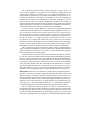
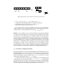
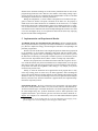
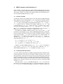
We consider standard, non-recursive C programs // Doubly-Linked Lists
manipulating dynamic linked data structures (with typedef struct {
DLL *next, *prev;
possibly several next pointer selectors). We do
} DLL;
not consider pointer arithmetics. We suppose all
non-pointer data to be abstracted to a finite doDLL *DLL_reverse(DLL *x) {
main by some of the existing techniques before
DLL *y,*z;
our method is applied. In the paper, we concenz = NULL;
trate on the following pointer manipulating program
y = x->next;
statements: x=NULL, x=y, x = y->next, x->next =
while (y!=NULL) {
y, x = malloc(), free(x), and if (x==y) goto
x->next = z;
x->prev = y;
L1; else goto L2; for pointer variables x and y
z = x; x = y;
and program line labels L1 and L2. We suppose some
y = x->next
further, commonly used statements (such as while
}
loops or nested dereferences) to be encoded by the
return x;
listed statements. For brevity, we do not explicitly
}
discuss manipulation of non-pointer finite-domain
Fig. 1. Reversing a DLL
data, which is anyway straightforward. An example
of a typical program that our method can handle is the reversion of doubly-linked lists
(DLL) shown in Fig. 1, which we also use as our running example.
2.2 The Considered Properties
First of all, the properties we intend to check include basic consistency of pointer manipulations, i.e. absence of null and undefined pointer dereferences and references to
already deleted nodes. Further, we would like to check various shape invariance properties (such as absence of sharing, acyclicity, or, e.g., the fact that if x->next == y
(and y is not null) in a DLL, then also y->prev == x, etc.). To define such properties
we propose two approaches described below.
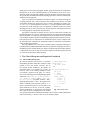
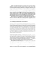
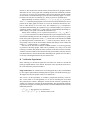
Shape Testers. First, we use the so-called shape
x = aDLLHead;
testers written in the C language. They can be seen
while (x != NULL && random())
as instrumentation code trying to detect violations
x = x->next;
of the memory shape properties at selected con- if (x != NULL
trol locations of the original program. We extend
&& x->next->prev != x)
slightly the C language used by the possibility of
error();
following next pointers backwards and by nondeterministic branching. For our verification tool, Fig. 2. Checking the consistency
the testers are just a part of the code being verified. of the next and previous pointers
An error is announced when a line denoted by an
error label is reached. This way, we can check a whole range of properties (including
acyclicity, absence of sharing and other shape invariants as the relation of next and
previous pointers in DLLs—cf. Fig 2).
A Logic of Bad Memory Patterns. Second, in order to allow the undesired violations
of the memory shape properties to be specified more easily, we propose a logic-based
specification language—namely, a logic of bad memory patterns (LBMP)—that is a
fragment of the existential first order logic on graphs with (regular) reachability predicates (and an implicit existential quantification over paths). When defining the logic,
our primary concern is not to obtain a decidable logic but rather to obtain a logic whose
formulae may be automatically translated to the above mentioned C testers allowing us
to efficiently test whether some bad shapes may arise from the given program by testing
reachability of a designated error control line of a tester.
Let V be a finite set of program variables and S a finite set of selectors. The formu/
lae of LBMP have the form Φ ::= ∃w1 , ...wn .ϕ where W = {w1 , ..., wn }, V ∩ W = 0,
is a set of formulae variables, ϕ ::= ϕ ∨ ϕ | ψ, ψ ::= ψ ∧ ψ | xρy, x, y ∈ V ∪ W , and ρ
is a reachability formula defined below. To simplify the formulae, we allow y in xρy to
be skipped if it is not referred to anywhere else. We suppose such a missing variable to
be implicitly added and existentially quantified. Given a ψ formula, we define its associated graph to be the graph Gψ = (V ∪ W , E) where (x, y) ∈ E iff xρy is a conjunct in
ψ. To avoid guessing in the tester corresponding to a formula, we require G ψ of every
top level ψ formula to have all nodes reachable from elements of V .
s s
An LBMP reachability formula has the form ρ ::=→|←| ρ + ρ | ρ.ρ | ρ∗ | [σ] where
s ∈ S and σ is a local neighbourhood formula. Finally, an LBMP local neighbours
hood formula has the form ∃u1 , ..., um .BC(x → y, x = y) where U = {u1 , ..., um } is
/ p 6∈ V ∪ W , s ∈ S , x ∈
a set of local formula variables, U ∩ (V ∪ W ∪ {p}) = 0,
V ∪ W ∪ U ∪ {p}, y ∈ V ∪ W ∪ U ∪ {p, ⊥, >}, and BC is the Boolean closure. Here, ⊥
represents NULL, > an undefined value, and p is a special variable that always represents
the current position in a shape graph. Moreover, to avoid guessing in the evaluation of
the local neighbourhood formulae, we require that if σ is transformed into σ 0 in DNF,
s
and we construct a graph based on the positive → literals for each disjunct of σ0 , each
node of such a graph is reachable from p.
The semantics of LBMP formulae is relatively straightforward. Therefore we defer
it description to Appendix A.1. Instead, we illustrate the semantics of LBMP formulae
on several examples expressing undesirable phenomena that we would like to avoid
when manipulating acyclic doubly-linked lists. In their case, it is undesirable if one
of the following happens after some operation (as, for instance, reversion) on a given
list—we suppose the resulting list to be pointed via the program variable l:
n ∗
1. the list does not end with null, which can be tested via l → [p = >],
b
2. the predecessor of the first element is not null, which corresponds to l[¬(p → ⊥)],
3. the predecessor of the successor of a node n is not n, which can be detected via the
p
n ∗
n
formula l → [∃x. p → x ∧ x 6= ⊥ ∧ ¬(x → p)], or
n ∗
n n ∗
4. the list is cyclic, i.e. ∃x. l → [p = x] →→ [p = x]. (Note that this property is in
fact implied by items 2 and 3.)
All the given formulae can be joint by disjunction into a single LBMP formula. Due
to the space limitations, we do not provide more examples of LBMP formulae, but we
note that for all the structures mentioned later in Section 5, we are able to specify all the
commonly considered undesirable situations in LBMP (some more examples of LBMP
formulae can then be found in Appendix B).
Due to a lack of space, the procedure for translating LBMP formulae is described
in Appendix B. Intuitively, it is quite easy to see that the existentially quantified LBMP
formulae with a stress on exploring paths through the examined linked data structures
starting from program variables can be encoded in a slightly extended C code, put after the program being verified, and used in an efficient way for checking safety of the
given program. We translate disjunctions to non-deterministic branching, conjunctions
and series of reachability formulae to series of tests, iteration in the reachability expressions to non-deterministic while loops. The needed extension of C includes nondeterministic branching and the possibility of following next pointers backwards. Both
of these features may easily be handled in our verification framework.
2.3 The Verification Problem
Our verification problem is model checking of the described undesirable existential
properties against the given program. Above, we explain that for the specification of
a violation of shape invariants, we use shape testers or LBMP whose formulae are
translated into shape testers. For shape testers, we need to check unreachability of their
designated error location. Moreover, we model all program statements such that if some
basic memory consistency error (like a null pointer assignment) happens, the control is
automatically transferred to a unique error control location. Thus, we are in general
interested in checking unreachability of certain error control locations in a program.
3 Automata-based Verification Framework
In this section, we introduce the abstract tree regular model-checking framework based
on tree automata and transducers that we use for solving our verification problem.
3.1 Tree Automata and Transducers
Terms and Trees. An alphabet Σ is a finite set of symbols. Σ is called ranked if there
exists a rank function ρ : Σ → N. For each k ∈ N, Σk ⊆ Σ is the set of all symbols with
rank k. Symbols of Σ0 are called constants. Let χ be a denumerable set of symbols
/ is denoted
called variables. TΣ [χ] denotes the set of terms over Σ and χ. The set TΣ [0]
by TΣ , and its elements are called ground terms. A term t from TΣ [χ] is called linear if
each variable occurs at most once in t.
A finite ordered tree t over a set of labels L is a mapping t : P os(t) → L where
P os(t) ⊆ N∗ is a finite, prefix-closed set of positions in the tree. A term t ∈ TΣ [χ] can
naturally also be viewed as a tree whose leaves are labelled by constants and variables,
and each node with k sons is labelled by a symbol from Σk [16]. Therefore, below, we
sometimes exchange terms and trees. We denote N lPos(t) = {p ∈ P os(t) | ¬∃i ∈ N :
pi ∈ P os(t)} the set of non-leaf positions.
Tree Automata. A bottom-up tree automaton over a ranked alphabet Σ is a tuple A =
(Q, Σ, F, δ) where Q is a finite set of states, F ⊆ Q is a set of final states, and δ is a
set of transitions of the following types: (i) f (q1 , . . . , qn ) →δ q, (ii) a →δ q, and (iii)
q →δ q0 where a ∈ Σ0 , f ∈ Σn , and q, q0 , q1 , . . . , qn ∈ Q. Below, we call a bottom-up tree
automaton simply a tree automaton.
Let t be a ground term. A run of a tree automaton A on t is defined as follows. First,
leaves are labelled with states. If a leaf is a symbol a ∈ Σ0 and there is a rule a →δ q ∈ δ,
the leaf is labelled by q. An internal node f ∈ Σk is labelled by q if there exists a rule
f (q1 , q2 , . . . , qk ) →δ q ∈ δ and the first son of the node has the state label q1 , the second
one q2 , ..., and the last one qk . Rules of the type q →δ q0 are called ε-steps and allow us
to change a state label from q to q0 . If the top symbol is labelled with a state from the
set of final states F, the term t is accepted by the automaton A.
A set of ground terms accepted by a tree automaton A is called a regular tree language and is denoted by L(A). Let A = (Q, Σ, F, δ) be a tree automaton and q ∈ Q a
state, then we define the language of the state q—L(A, q)—as the set of ground terms
accepted by the tree automaton Aq = (Q, Σ, {q}, δ). The language L≤n (A, q) is defined
to be the set {t ∈ L(A, q) | height(t) ≤ n}.
Tree Transducers. A bottom-up tree transducer is a tuple τ = (Q, Σ, Σ0 , F, δ) where
Q is a finite set of states, F ⊆ Q a set of final states, Σ an input ranked alphabet, Σ0
an output ranked alphabet, and δ a set of transition rules of the following types: (i)
f (q1 (x1 ), . . . , qn (xn )) →δ q(u), u ∈ TΣ0 [{x1 , . . . , xn }], (ii) q(x) →δ q0 (u), u ∈ TΣ0 [{x}], and
(iii) a →δ q(u), u ∈ TΣ0 where a ∈ Σ0 , f ∈ Σn , x, x1 , . . . , xn ∈ χ, and q, q0 , q1 , . . . , qn ∈ Q. In
the following, we call a bottom-up tree transducer simply a tree transducer. We always
use tree transducers with Σ = Σ0 .
A run of a tree transducer τ on a ground term t is similar to a run of a tree automaton
on this term. First, rules of type (iii) are used. If a leaf is labelled by a symbol a and there
is a rule a →δ q(u) ∈ δ, the leaf is replaced by the term u and labelled by the state q. If a
node is labelled by a symbol f , there is a rule f (q1 (x1 ), q2 (x2 ), . . . , qn (xn )) →δ q(u) ∈ δ,
the first subtree of the node has the state label q1 , the second one q2 , . . ., and the last one
qn , then the symbol f and all subtrees of the given node are replaced according to the
right-hand side of the rule with the variables x1 , . . . , xn substituted by the corresponding
left-hand-side subtrees. The state label q is assigned to the new tree. Rules of type (ii)
are called ε-steps. They allow us to replace a q-state-labelled tree by the right hand side
of the rule and assign the state label q0 to this new tree with the variable x in the rule
substituted by the original tree. A run of a transducer is successful if the root of a tree
is processed and is labelled by a state from F.
A tree transducer is linear if all right-hand sides of its rules are linear (no variable
occurs more than once). The class of linear bottom-up tree transducers is closed under
composition. A tree transducer is called structure-preserving (or a relabelling) if it does
not modify the structure of input trees and just changes the labels of their nodes. By
abuse of notation, we identify a transducer τ with the relation {(t,t 0 ) ∈ TΣ × TΣ | t →∗δ
q(t 0 ) for some q ∈ F}. For a set L ⊆ TΣ and a relation R ⊆ TΣ × TΣ , we denote R(L) the
set {w ∈ TΣ | ∃w0 ∈ L : (w0 , w) ∈ R} and R−1 (L) the set {w ∈ TΣ | ∃w0 ∈ L : (w, w0 ) ∈ R}.
If τ is a linear tree transducer and L is a regular tree language, then the sets τ(L) and
τ−1 (L) are regular and effectively constructible [19, 16].
Let id ⊆ TΣ × TΣ be the identity relation and ◦ the composition of relations. We
i
define recursively the relations τ0 = id, τi+1 = τ◦τi and τ∗ = ∪∞
i=0 τ . Below, we suppose
i
i+1
id ⊆ τ meaning that τ ⊆ τ for all i ≥ 0.
3.2 Abstract Regular Tree Model Checking
Let us recall the basic principles of abstract regular tree model checking (ARTMC) [9].
Let Σ be a ranked alphabet and MΣ the set of all tree automata over Σ. Let Init ∈ MΣ be
a tree automaton describing a set of initial configurations, τ a tree transducer describing
the behaviour of a system, and Bad ∈ MΣ a tree automaton describing a set of bad
configurations. The verification problem is to check whether
τ∗ (L(Init)) ∩ L(Bad) = 0/
(1)
One of the methods how to check this is ARTMC [9]. Instead of computing the precise
set of reachable configurations, it computes an overapproximation.
We define an abstraction function as a mapping α : MΣ → AΣ where AΣ ⊆ MΣ and
∀M ∈ MΣ : L(M) ⊆ L(α(M)). An abstraction α0 is called a refinement of the abstraction
α if ∀M ∈ MΣ : L(α0 (M)) ⊆ L(α(M)). Given a tree transducer τ and an abstraction α,
we define a mapping τα : MΣ → MΣ as ∀M ∈ MΣ : τα (M) = τ̂(α(M)) where τ̂(M) is
the minimal deterministic automaton describing the language τ(L(M)). An abstraction
α is finitary, if the set AΣ is finite.
For a given abstraction function α, we can compute iteratively the sequence of
automata (τiα (Init))i≥0 . If the abstraction α is finitary, then there exists k ≥ 0 such
k
that τk+1
α (Init) = τα (Init). The definition of the abstraction function α implies, that
k
∗
L(τα (Init)) ⊇ τ (L(Init)).
/ then the verification problem (1) has a positive answer.
If L(τkα (Init)) ∩ L(Bad) = 0,
If the intersection is non-empty, we must check whether it is a real counterexample,
or a spurious one. The spurious counterexample may be caused by the used abstraction
(the counterexample is not reachable from the set of initial configurations). Assume that
/ which means that there is a symbolic path:
τkα (Init) ∩ L(Bad) 6= 0,
n
Init, τα (Init), τ2α (Init), · · · τn−1
α (Init), τα (Init)
(2)
/
such that L(τnα (Init)) ∩ L(Bad) 6= 0.
Let Xn = L(τnα (Init)) ∩ L(Bad). Now, for each l, 0 ≤ l < n, we compute Xl =
/ which means that
L(τlα (Init)) ∩ τ−1 (Xl+1 ). Two possibilities may occur: (a) X0 6= 0,
the verification problem (1) has a negative answer, and X0 ⊆ L(Init) is a set of dangerous initial configurations. (b) ∃m, 0 ≤ m < n, Xm+1 6= 0/ ∧ Xm = 0/ meaning that the
abstraction function is too rough—we need to refine it and start the verification process
again.
In [9], two general-purpose kinds of abstractions are proposed. Both are based on
automata state equivalences. Tree automata states are split into several equivalence
classes, and all states from one class are collapsed into one state. An abstraction becomes finitary if the number of equivalence classes is finite. The refinement is done by
refining the equivalence classes. Both of the proposed abstractions allow for an automatic refinement to exclude the encountered spurious counterexample.
The first proposed abstraction is an abstraction based on languages of trees of a finite height. It defines two states equivalent if their languages up to the give height n are
equivalent. There is just a finite number of languages of height n, therefore this abstraction is finitary. A refinement is done by an increase of the height n. The second proposed
abstraction is an abstraction based on predicate languages. Let P = {P1 , P2 , . . . , Pn } be
a set of predicates. Each predicate P ∈ P is a tree language represented by a tree automaton. Let M = (Q, Σ, F, δ) be a tree automaton. Then, two states q1 , q2 ∈ Q are equivalent
if their languages L(M, q1 ) and L(M, q2 ) have a nonempty intersection with exactly the
same subset of predicates from the set P . Since there is just a finite number of subsets
of P , the abstraction is finitary. A refinement is done by adding new predicates, i.e. tree
automata corresponding to the languages of all the states in the automaton of Xm+1 from
/
the analysis of spurious counterexample (Xm = 0).
4 Tree Automata Encoding of Pointer Manipulating Programs
4.1 Encoding of Sets of Memory Configurations
Memory configurations of the considered programs with a finite set of pointer variables
V , a finite set of selectors S = {1, ..., k}, and a finite domain D of data stored in dynamically allocated memory cells can be described as shape graphs of the following form.
A shape graph is a tuple SG = (N, S,V, D) where N is a finite set of memory nodes,
N ∩ {⊥, >} = 0/ (we use ⊥ to represent null, and > to represent an undefined pointer
value), N⊥,> = N ∪ {⊥, >}, S : N × S → N⊥,> is a successor function, V : V → N⊥,>
is a mapping that defines where the pointer variables are currently pointing to, and
D : N → D defines what data are stored in the particular memory nodes. We suppose
> ∈ D —the data value > is used to denote “zombies” of deleted nodes, which we keep
and detect all erroneous attempts to access them.
To be able to describe the way we encode sets of shape graphs using tree automata,
we first need a few auxiliary notions. First, to allow for dealing with more general shape
graphs than tree-like, we do not simply identify the next pointers with the branches of
the trees accepted by tree automata. Instead, we use the tree structure just as a backbone
over which links between the allocated nodes are expressed using the so-called routing
expressions, which are regular expressions over directions in a tree (like move up, move
left down, etc.) and over the nodes that can be seen on the way. From nodes of the
trees described by tree automata, we refer to the routing expressions via some symbolic
names called pointer descriptors that we assign to them—we suppose dealing with a
finite set of pointer descriptors R . Moreover, we couple each pointer descriptor with a
unique marker from a set M (and so ||R || = ||M ||). The routing expressions may identify several target nodes for a single source memory node and a single selector. Markers
associated with the target nodes can then be used to decrease the non-determinism of
the description (only nodes marked with the right marker are considered as the target).
Let us now fix the sets V , S , D , R , and M . We use a ranked alphabet Σ =
Σ2 ∪ Σ1 ∪ Σ0 consisting of symbols of ranks k = ||S ||, 1, and 0. Symbols of rank k
represent allocated memory nodes that may be pointed by some pointer variables, may
be marked by some markers as targets of some next pointers, they contain some data
and have k next pointers specified either as null, undefined, or via some next pointer descriptor. Thus, Σ2 = 2V × 2M × D × (R ∪ {⊥, >})k . Given an element n ∈ Σ2 , we use
the notation n.var, n.mark, n.data, and n.s (for s ∈ S ) to refer to the pointer variables,
markers, data, and descriptors associated with n, respectively. Σ 1 is used for specifying
nodes with undefined and null pointer variables, and so Σ1 = 2V . Finally, in our trees,
the leaves are all the same (with no special meaning), and so Σ0 = {•}.
We can now specify the tree memory backbones we use to encode memory configurations as the trees that belong to the language of the tree automaton with the following rules3 : (1) • → qi , (2) Σ2 (qi /qm , ..., qi /qm ) → qm , (3) Σ1 (qm /qi ) → qn , and (4)
Σ1 (qn ) → qu . Intuitively, qi , qm , qn , and qu are automata states, where qi accepts the
leaves, qm accepts the memory nodes, qn accepts the node encoding null variables, and
qu , which is the accepting state, accepts the node with undefined variables. Note that
there is always a single node with undefined variables, a single node with null variables, and then a sub-tree with the memory allocated nodes. Thus, every memory tree
t can be written as t = undef (null(t 0 )) for undef , null ∈ Σ1 . We say a memory tree
t = undef (null(t 0 )) is well-formed if the pointer variables are assigned unique meanings, i.e. undef ∩ null = 0/ ∧ ∀p ∈ N lPos(t 0 ) : t 0 (p).var ∩ (null ∪ undef ) = 0/ ∧ ∀p1 6=
p2 ∈ N lPos(t 0 ) : t 0 (p1 ).var ∩ t 0 (p2 ).var = 0/ where N lPos are non-leaf positions—cf.
Section 3.1.
We let S −1 = {s−1 | s ∈ S } be a set of “inverted selectors” allowing one to follow
the links in a shape graph in a reverse order. A routing expression may then be formally
defined as a regular expression on pairs s.p ∈ (S ∪ S−1 ).Σ2 . Intuitively, each pair used as
3
If we put a set into the place of the input symbol in a transition rule, we mean we can use any
element of the set. Moreover, if we use q1 /q2 instead of a single state, one can take either q1
or q2 , and if there is a k-tuple of states, one considers all possible combinations of states.
The original DLL
A tree memory encoding of the DLL
undefined pointers
null
Y
Descriptors
S = {1, 2}
−1
S = {1, 2}
D1 : 1. M1
null pointers
X null
7
X
14
26
M2
Z
Z
M1 M2 26
D2 : 1. M2
D1
7
D2
D1
M1 M2 14
Y
D2
D1
10
M1
10
D2
null
Fig. 3. An example of a tree memory encoding—a doubly linked list (DLL)
a basic building block of a routing expression describes one step over the tree memory
backbone: we follow a certain branch up or down and then we should see a certain node
(most often, we will use the node components of routing expressions to check whether
a certain marker is set in a particular node).
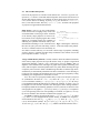
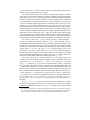
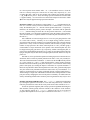
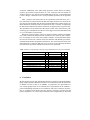
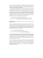
A tree memory encoding is a tuple (t, µ) where t is a tree memory backbone and
µ a mapping from the set of pointer descriptors R to routing expressions over the set
of selectors S and the memory node alphabet Σ2 of t. An example of a tree memory
encoding for a doubly-linked list (DLL) is shown in Fig. 3.
Let (t, µ), t = undef (null(t 0 )), be a tree memory encoding with a set of selectors
S and a memory node alphabet Σ2 . We call π = p1 s1 ...pl sl pl+1 ∈ Σ2 .((S ∪ S −1 ).Σ2 )l
a path in t of length l ≥ 1 iff p1 ∈ P os(t 0 ) and ∀i ∈ {1, ..., l} : (si ∈ S ∧ pi .si = pi+1 ∧
pi+1 ∈ P os(t 0 )) ∨ (si ∈ S −1 ∧ pi+1 .si = pi ). For p, p0 ∈ N lPos(t 0 ) and a selector s ∈ S ,
s
we write p −→ p0 iff (1) t 0 (p).s ∈ R , (2) there is a path p1 s1 ...pl sl pl+1 in t for some
l ≥ 0 such that p = p1 , pl+1 = p0 , and (3) s1t 0 (p2 )...t 0 (pl )sl t 0 (pl+1 ) ∈ µ(t 0 (p).s).
The set of shape graphs represented by a tree memory encoding (t, µ) with t =
undef (null(t 0 )) is denoted by [[(t, µ)]] and given as all the shape graphs SG = (N, S,V, D)
for which there is a bijection β : P os(t 0 ) → N such that:
1. ∀p, p0 ∈ N lPos(t 0 ) ∀s ∈ S : (t 0 (p).s 6∈ {⊥, >} ∧ p −→ p0 ) ⇔ S(β(p), s) = β(p0 ).
(The links between memory nodes are respected.)
2. ∀p ∈ N lPos(t 0 ) ∀s ∈ S ∀x ∈ {⊥, >} : t 0 (p).s = x ⇔ S(β(p), s) = x.
(Null and undefined successors are respected.)
3. ∀v ∈ V ∀p ∈ P os(t 0 ) : v ∈ t 0 (p).var ⇔ V (v) = β(p).
(Assignment of memory nodes to variables is respected.)
s
pointers markers
pointers markers
data
D1
D2
...
data
Dn
D1
D2
Subtree 1
Subtree 2
...
...
Subtree n
Dn
Subtree 1
Subtree 2
Subtree n
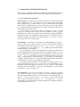
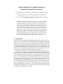
Fig. 4. Splitting memory nodes in Mona into data and next pointer nodes
4. ∀v ∈ V : (v ∈ null ⇔ V (v) = ⊥) ∧ (v ∈ undef ⇔ V (v) = >).
(Assignment of null and undefinedness of variables are respected.)
5. ∀p ∈ N lPos(t 0 ) ∀d ∈ D : t 0 (p).data = d ⇔ D(β(p)) = d.
(Data stored in memory nodes is respected.)
A tree automata memory encoding is a tuple (A, µ) where A is a tree automaton accepting a regular set of tree memory backbones and µ is a mapping as above. Naturally,
S
A represents the set of shape graphs defined by [[(A, µ)]] = t∈L(A) [[(t, µ)]].
Remarks. We use ARTMC as our verification method. It syntactically manipulates
tree automata A whose languages can be interpreted as shape graphs using our encoding. Notice, that (A, µ) and [[(A, µ)]] are two different notions, since the encoding is
not canonical as a given shape graph can be possibly obtained by several different tree
memory encodings. In Section 4.3, we argue that program statements can, nevertheless,
be encoded faithfully as tree transducers. Another important property of the encoding
is that given a tree automata memory encoding (A, µ), the set [[(A, µ)]] can be empty
although L(A) is not empty (since the routing expressions can be incompatible with the
tree automaton). Of course, if L(A) is empty, then [[(A, µ)]] is also empty. Therefore,
checking emptiness of [[(A, µ)]] (which is important for applying the ARTMC framework, see Section 4.4) can be done in a sound way by checking emptiness of L(A).
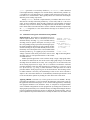
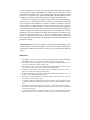
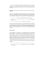
4.2 Tree Memory Configurations in Mona
In our implementation, we use the tree automata library from the Mona project [23]. As
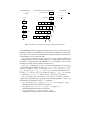
the library supports binary trees only, and we need n-ary ones, we split each memory
node labelled with Σ2 = 2V × 2M × D × (R ∪ {⊥, >})k in the above definition of a tree
memory encoding into a data node labelled with 2V × 2M × D and a series of k next
pointer nodes, each labelled with R ∪ {⊥, >}—cf. Fig. 4.
As for the set of pointer descriptors R , we currently fix it by introducing a unique
pointer descriptor for each destructive update x->s = y or x->s = new that appears in
the program. This is because they are the statements that establish new links among the
allocated memory nodes. In addition, we might have some further descriptors if they
are a part of the specification of the input configurations (see section 4.4).
Further, in our Mona-based framework, we encode routing expressions using tree
transducers. A transducer representing a routing expression r simply copies the input
tree memory backbone on which it is applied up to: (1) looking for a data node n 1 that is
labelled with a special token 6∈ V ∪ M ∪ D and (2) moving to a data node n 2 that is
the target of the next pointer described by r and that is also marked with the appropriate
marker. As described in the next section, we can then implement program statements
that follow the next pointers (e.g., x = y->s) by putting the token to a node pointed
to by x, applying the transducer implementing the appropriate routing expression, and
making y point to the node to which was moved. Due to applying abstraction, the target may not always be unique—in such a case, the transducer implementing the routing
expression simply returns a set of trees in which is put to some target data node such
that all possibilities where it can get via the given routing expression are covered.
Note that the use of tree transducers for encoding routing expressions allows us
in theory to express more than using just regular expressions. In particular, we can
refer to the tree context of the nodes via which the given route is going. In our current
implementation, we, however, do not use this fact.
4.3 Encoding Program Statements as Tree Transducers
We encode every of the considered pointer-manipulating statements as a tree transducer.
In the transducer, we expect the tree memory encoding to be extended by a new root
symbol which corresponds to the current program line or to an error indication when
an error is found during the analysis. We now briefly describe how the transducers
corresponding to the program statements work. Each transducer is constructed in such
a way, that it simulates the effect of a program statement on a set of shape graphs
represented by a tree automata memory encoding: if a shape SG represented by a tree
memory encoding is transformed by the program statement to a shape graph SG 0 , then
the transducer transforms the tree memory encoding such that it represents SG 0 . This
makes sure, that although the encoding is non canonical (see end of section 4.1), we
simulate faithfully a program statement.
Non-destructive Updates and Tests. The simplest is the case of the x = NULL assignment. The transducer implementing it just goes through the input tree and copies it
to the output with the exception that (1) it removes x from the labelling of the node in
which it currently is and adds it to the labelling of the null node and (2) changes the current line appropriately. The transducer implementing an assignment x = y is similar, it
just puts x not to the null node, but to the node which is currently labelled by y.
The transducers for the tests of the form if (x == null) goto l1; else goto
l2; are very similar to the above—they just do not change the node in which x is, but
only change the current program line to either l1 or l2 according to whether or not
x is in the null node. If x is in undef , an error indication is used instead of l1 or l2.
The transducers for if (x == y) goto l1; else goto l2; are similar—they just
test whether or not x and y appear in the same node (both different from undef ).
The transducer for an x = y->s statement is a union of several complementary
actions. If y is in null or undef , an error is indicated. If y is in a regular data node and
its s-th next pointer node contains either ⊥ or >, the transducer removes x from the
node it is currently in and puts it into the null or undef node, respectively. If y is in
a regular data node n and its s-th next pointer node contains some pointer descriptor
r ∈ R , the token is put to n. Then, the routing expression transducer associated with
r is applied. Finally, x is removed from its current node and put into the node to which
was moved by the applied routing expression transducer.
Destructive Updates. The destructive pointer update x->s = y is implemented as follows. If x is in null or undef , an error is indicated. If x is defined and if y is in null or
undef , the transducer puts ⊥ or > into the s-th next pointer node below x, respectively.
Otherwise, the transducer puts the pointer descriptor r associated with the particular
x->s = y statement being fired into the s-th next pointer node below x, and it marks
the node in which y is by the marker coupled with r. Then, the routing expression transducer associated with r is updated such that it includes the path from the node of x to
the node of y.
One could think of various strategies how to extract the path going from the node
of x to the node of node y. Currently, we use a simple strategy, which is, however,
successful in many practical examples as our experiments show: We extract the shortest
path between x and y on the tree memory backbone, which consists of going a certain
number of steps upwards to the closest common parent of x and y and then going a
certain number of steps downwards. (The upward or the downward phase may also
be skipped when going just down or up, respectively.) When extracting this path, we
project away all information about nodes we see on the way and about nodes not directly
lying on the path. Only the directions (left/right up/down) and the number of steps are
preserved.
Note that we, in fact, perform the operation of routing expression extraction on a tree
automaton, and we extract all possible paths between where x and y may currently be.
The result is transformed into a transducer τxy that moves the token from the position
of x to the position of y, and τxy is then united with the current routing expression
transducer associated with the given pointer descriptor r. The extraction of the routing
paths is done partly by rewriting the input tree automaton via a special transducer τ π
that in one step identifies all the shortest paths between all x and y positions and projects
away the non-necessary information about the nodes on the way. The transducer τ π is
simple: it just checks that we are going one branch up from x and one branch down to y
while meeting in a single node. The transition relation of the resulting transducer is then
post-processed by changing the context of the path to an arbitrary one which cannot be
done by transducing in Mona where structure preserving transducers may only be used.
Dynamic Allocation and Deallocation. The x = malloc() statement is implemented
by rewriting the right-most • leaf node to a new data node pointed to by x. Below the
node, the procedure also creates all the k next pointer nodes whose contents is set to >.
In order to exploit the regularity that is always present in algorithms allocating new
data structures, which typically add new elements at the end/leaves of the structure,
we also explicitly support an x.s = malloc() statement. We even try to pre-process
programs and compact all successive pairs of statements of the form x = malloc();
y->s = x (provided x is not used any further) to y->s= malloc(). Such a statement
is then implemented by adding the new element directly under the node pointed to by
y (provided it is a leaf) and joining it by a simple routing expression of the form “one
level down via a certain branch”. This typically allows us to work with much simpler
and more precise routing expressions.
Finally, a free(x) statement is implemented by a transducer that moves all variables that are currently in the node pointed to by x to the undef node (if x is in null or
undef , an error is indicated). Then, the node is marked by a special marker as a deleted
node, but it stays in our tree memory encoding with all its current markers set. In addition to all the other tests mentioned above as done within the transducer implementing
an x = y->s assignment, it is also tested whether the target is not deleted—if so, an
error is indicated.
4.4 Verification of Programs with Pointers using ARTMC
Input structures. We consider two possibilities how to enaDLLHead = malloc();
code the input structures. First, we can directly use the tree
aDLLHead->prev = null;
automata memory encoding—e.g., a tree automata memory x = aDLLHead;
encoding (with two pointer descriptors next and prev and while (random()) {
the corresponding routing expressions) describing all possix->next = malloc();
ble doubly-linked lists pointed to by some program variable.
x->next->prev = x;
Such an encoding can be provided manually or derived aux = x->next;
tomatically from a description of the concerned linked data }
structure provided, e.g., as a graph type [24]. The main ad- x->next = null;
vantage is that the verification process starts with an exact Fig. 5. Generating DLLs
encoding of the set of all possible instances of the considered data structure.
Another possible approach is to start with the unique “empty” shape graph where
all variables are undefined. We can encode such a shape graph using a tree automata
encoding where all variables are in undef , null is empty, there are no other nodes, and
all the routing expressions are empty. The set of structures on which the examined
procedure should be verified is then supposed to be generated by a constructor written
in C by the user (as, e.g., in Fig. 5). This constructor is then put before the verified
procedure and the whole program is given to the model checker. The advantage is that
no further notation is necessary. The disadvantage is that we have more code that is
subject to the verification and the set of automatically obtained input structures need
not be encoded in the optimal way leading to a slow-down of the verification.
Applying ARTMC. In Section 3.2, we have given an overview of ARTMC. We supposed that one transducer τ is used to describe the behaviour of the whole system. In
the application described in this paper, we use a variant of this approach by considering
each program statement as one transducer. Then, we compute an overapproximation
of the reachable configurations for each program line by starting from an initial set of
shape graphs represented by a tree automata memory encoding and iterating the abstract
fixpoint computation described in Section 3.2 through the program structure. The fixpoint computation stops if the abstraction α is finitary. In such a case, the number of the
abstracted tree automata encoding sets of the memory backbones that can arise in the
program being checked is finite. Moreover, the number of the arising routing expressions is also finite as they are extracted from the bounded number of the tree automata
describing the encountered sets of memory backbones.4
During the computation, we check whether a designated error location in the program is reached or whether a fixpoint is attained. In the latter case, the property is
satisfied (the error control location is not reachable). In the former case, we compute
backwards to check if the counterexample is spurious as explained in Section 3.2. However, as said in Section 4.1, the check for emptiness is not exact and therefore we might
conclude that we have obtained a real counterexample although this is not the case. Such
a case does not happen in any of our experiments and could be detected by replaying
the path from the initial configurations.
5 Implementation and Experimental Results
An ARTMC Tool for Tree Automata Memory Encodings. We have implemented the
above proposed method in a prototype tool based on the Mona tree automata libraries
[23]. We use a depth-first strategy when iterating the transducers corresponding to the
particular program lines.
We have also refined the basic finite-height and predicate abstractions proposed in
[9]. In particular, we do not allow collapsing of data nodes with next pointer nodes,
collapsing of next pointer nodes corresponding to different selectors, and we prevent
the abstraction of allowing a certain pointer variable to point to several memory nodes
at the same time. Experiments showed, that it is better to collaps only at data nodes.
We have also proposed one new abstraction schema called the neighbour abstraction. Under this schema, only the tree automata states are collapsed that (1) accept equal
data memory nodes with equal next pointer nodes associated with them and (2) that directly follow each other (are neighbours). This strategy is very simple, yet it proved
useful in some practical cases.
Finally, we allow the abstraction to be applied either at all program lines or only
at the loop closing points. In some cases, the latter approach is more advantageous
due to some critical destructive pointer updates are done without being interleaved with
abstraction. This way, we may avoid having to remove lots of spurious counterexamples
that may otherwise arise when the abstraction is applied while some important shape
invariant is temporarily broken.
Experimental Results. We have performed several experiments with singly-linked
lists (SLL), doubly-linked lists (DLL), trees, lists of lists, and trees with linked leaves.
All three mentioned types of automata abstraction—the finite height abstraction (with
the initial height being one), predicate abstraction (with no initial predicates), and
neighbour abstraction—proved useful (gave the best achieved result) in different examples. All examples were automatically verified for null/undefined/deleted pointer
4
The non-canonicity of our encoding does not prevent the computation from stopping. It may
just take longer since several encodings for the same graph could be added.
exceptions. Additionally, some further shape properties (such as absence of sharing,
acyclicity, preservation of input elements, etc.) were verified in some case studies too.
All these properties were specified in the LBMP logic from Sect. 2.2 and translated to
C testers. We give a detailed overview of the performed experiments in the Appendix
B.
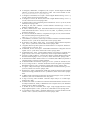
Table 1 contains verification times for the experiments mentioned above (the “+
test” in the name of an experiment means that some shape invariants were checked). We
give the best result obtained using the three mentioned abstraction schemas and say for
which abstraction schema the result was obtained. The note “restricted” accompanying
the abstraction method means that the abstraction was applied at the loop points only.
The experiments were performed on a 64bit Xeon 3,2 GHz with 3 GB of memory. The
column |Q| gives information about the size of the biggest encountered automaton, and
Nre f gives the number of refinements.
Despite the prototype nature of the tool, which can still be optimised in multiple
ways (some of them are mentioned in the conclusions), the results are quite competitive. For example, for one of the most complex examples—the Deutsch-Schorr-Waite
tree traversal, TVLA took 3 minutes on the same machine with manually provided instrumentation predicates and predicate transformers. The verification time for the trees
with linked leaves is relatively high, but we are not aware of any other fully automated
tool with which experiments with this structure have been performed.
Table 1. Results of experimenting with the prototype implementation of the presented method
Example
SLL-creation + test
SLL-reverse + test
DLL-delete + test
DLL-insert + test
DLL-reverse + test
DLL-insertsort
Inserting into trees + test
Linking leaves in trees + test
Inserting into a list of lists + test
Deutsch-Schorr-Waite tree traversal
Time
1s
5s
6s
10s
8s
2s
29s
49s
6s
57s
Abstraction method |Q| Nre f
predicates, restricted 25 0
predicates
52 0
finite height
100 0
neighbour, restricted 106 0
predicates
54 0
predicates
51 0
predicates, restricted 65 0
predicates
75 2
predicates, restricted 55 0
predicates
126 0
6 Conclusion
We have proposed a new, fully automated method for verification of programs manipulating complex dynamic linked data structures. The method is based on the framework
of ARTMC. In order to able to use ARTMC, we proposed a new representation of
sets of shape graphs based on tree automata and a representation of the standard C
pointer manipulating statements as tree transducers (with some extensions). In particular, we considered verification of the basic memory consistency properties (no null
pointer assignments, etc.) and of shape invariants whose corruption may be described
in an existential fragment of a first-order logic on graphs. We formalised this fragment
as a special-purpose logic called LBMP whose formulae may be translated to C-based
testers that may be attached to the verified programs, thus transforming the verification
problem to be considered to the control line reachability. We have implemented the
technique in a prototype tool and obtained some promising experimental results.
In the future, we would like to optimise the performance of our Mona-based prototype tool, e.g., by exploiting the concept of guided tree automata that are suggested
as very helpful in many situations by the authors of Mona [5] and that we have not
used yet. Further, it is interesting to try come up with some special purpose automata
abstractions for the considered domain—so-far we have used mostly general purpose
tree automata abstractions, and we have an experience from [8] that special purpose abstraction may bring very significant speed-ups (in [8], it was sometimes two orders of
magnitude or even more). Further research directions then include, for instance, checking of other kinds of properties (as, e.g., absence of garbage, which we know to be
possible—cf. Appendix C, but which we have not yet implemented), experimenting
with combinations of our technique with techniques of non-pointer data abstraction, or
termination checking.
Acknowledgement. This work was supported in part by the French Ministry of Research (ACI project Securité Informatique), by the Czech Grant Agency within projects
102/05/H050, 102/04/0780, 102/03/D211, and by the Czech-French project Barrande
2-06-27.
References
1. P.A. Abdulla, J. d’Orso, B. Jonsson, and M. Nilsson. Regular Model Checking Made Simple
and Efficient. In Proc. of CONCUR’02, volume 2421 of LNCS. Springer, 2002.
2. P.A. Abdulla, B. Jonsson, P. Mahata, and J. d’Orso. Regular Tree Model Checking. In Proc.
of CAV’02, volume 2404 of LNCS. Springer, 2002.
3. P.A. Abdulla, A. Legay, J. d’Orso, and A.Rezine. Simulation-Based Iteration of Tree Transducers. In Proc. of TACAS’05, volume 3440 of LNCS. Springer, 2005.
4. I. Balaban, A. Pnueli, and L. Zuck. Shape Analysis by Predicate Abstraction. In Proc. of
VMCAI’05, volume 3385 of LNCS. Springer, 2005.
5. M. Biehl, N. Klarlund, and T. Rauhe. Algorithms for Guided Tree Automata. In Proc. of
WIA’96, volume 1260 of LNCS. Springer, 1997.
6. B. Boigelot, A. Legay, and P. Wolper. Iterating Transducers in the Large. In Proc. of CAV’03,
volume 2725 of LNCS. Springer, 2003.
7. A. Bouajjani, M. Bozga, P. Habermehl, R. Iosif, P. Moro, and T. Vojnar. Programs with Lists
are Counter Automata. Technical Report TR-2006-3, Verimag, UJF/CNRS/INPG, Grenoble,
2006.
8. A. Bouajjani, P. Habermehl, P. Moro, and T. Vojnar. Verifying Programs with Dynamic 1Selector-Linked Structures in Regular Model Checking. In Proc. of TACAS’05, volume 3440
of LNCS. Springer, 2005.
9. A. Bouajjani, P. Habermehl, A. Rogalewicz, and T. Vojnar. Abstract Regular Tree Model
Checking. ENTCS, 149:37–48, 2006. A preliminary version was presented at Infinity’05.
10. A. Bouajjani, P. Habermehl, A. Rogalewicz, and T. Vojnar. Abstract Regular Tree Model
Checking of Complex Dynamic Data Structures, 2006. Full version available on URL:
http://www.fit.vutbr.cz/˜vojnar/pubs.php.
11. A. Bouajjani, P. Habermehl, and T. Vojnar. Abstract Regular Model Checking. In Proc. of
CAV’04, volume 3114 of LNCS. Springer, 2004.
12. A. Bouajjani, B. Jonsson, M. Nilsson, and T. Touili. Regular Model Checking. In Proc. of
CAV’00, volume 1855 of LNCS. Springer, 2000.
13. A. Bouajjani and T. Touili. Extrapolating Tree Transformations. In Proc. of CAV’02, volume
2404 of LNCS. Springer, 2002.
14. M. Bozga, R. Iosif, and Y. Lakhnech. Storeless Semantics and Alias Logic. In Proc. of
PEPM’03. ACM Press, 2003.
15. M. Češka, P. Erlebach, and T. Vojnar. Pattern-Based Verification of Programs with Extended
Linear Linked Data Structures. ENTCS, 145:113–130, 2006. A preliminary version was
presented at AVOCS’05.
16. H. Comon, M. Dauchet, R. Gilleron, F. Jacquemard, D. Lugiez, S. Tison, and M. Tommasi.
Tree Automata Techniques and Applications, 2005.
URL: http://www.grappa.univ-lille3.fr/tata.
17. J.V. Deshmukh, E.A. Emerson, and P. Gupta. Automatic Verification of Parameterized Data
Structures. In Proc. of TACAS’06, volume 3920 of LNCS. Springer, 2006.
18. D. Distefano, P.W. O’Hearn, and H. Yang. A Local Shape Analysis Based on Separation
Logic. In Proc. of TACAS’06, volume 3920 of LNCS. Springer, 2006.
19. J. Engelfriet. Bottom-up and Top-down Tree Transformations—A Comparison. Mathematical System Theory, 9:198–231, 1975.
20. P. Habermehl, R. Iosif, and T. Vojnar. Automata-Based Verification of Programs with Tree
Updates. In Proc. of TACAS’06, volume 3920 of LNCS. Springer, 2006.
21. P. Habermehl and T. Vojnar. Regular Model Checking Using Inference of Regular Languages. ENTCS, 138:21–36, 2005. A preliminary version was presented at Infinity’04.
22. Y. Kesten, O. Maler, M. Marcus, A. Pnueli, and E. Shahar. Symbolic Model Checking with
Rich Assertional Languages. In Proc. of CAV’97, volume 1254 of LNCS. Springer, 1997.
23. N. Klarlund and A. Møller. MONA Version 1.4 User Manual, 2001. BRICS, Department of
Computer Science, University of Aarhus, Denmark.
24. N. Klarlund and M.I. Schwartzbach. Graph Types. In Proc. of POPL’93. ACM Press, 1993.
25. O. Lee, H. Yang, and K. Yi. Automatic Verification of Pointer Programs Using GrammarBased Shape Analysis. In Proc. of ESOP’05, volume 3444 of LNCS. Springer, 2005.
26. A. Loginov, T. Reps, and M. Sagiv. Abstraction Refinement via Inductive Learning. In Proc.
of CAV’05, volume 3576 of LNCS. Springer, 2005.
27. R. Manevich, E. Yahav, G. Ramalingam, and M. Sagiv. Predicate Abstraction and Canonical
Abstraction for Singly-Linked Lists. In Proc. of VMCAI’05, volume 3385 of LNCS. Springer,
2005.
28. A. Møller and M.I. Schwartzbach. The Pointer Assertion Logic Engine. In Proc. of PLDI’01.
ACM Press, 2001. Also in SIGPLAN Notices 36(5), 2001.
29. S. Sagiv, T.W. Reps, and R. Wilhelm. Parametric Shape Analysis via 3-valued Logic.
TOPLAS, 24(3), 2002.
30. E. Shahar and A. Pnueli. Acceleration in Verification of Parameterized Tree Networks. Technical Report MCS02-12, Faculty of Mathematics and Computer Science, The Weizmann
Institute of Science, Rehovot, Israel, 2002.
31. A. Vardhan, K. Sen, M. Viswanathan, and G. Agha. Using Language Inference to Verify
Omega-regular Properties. In Proc. of TACAS’05, volume 3440 of LNCS. Springer, 2005.
32. T. Yavuz-Kahveci and T. Bultan. Automated Verification of Concurrent Linked Lists with
Counters. In Proc. of SAS’02, volume 2477 of LNCS. Springer, 2002.
33. G. Yorsh, A. Rabinovich, M. Sagiv, A. Meyer, and A. Bouajjani. A Logic of Reachable Patterns in Linked Data-Structures. In Proc. of FOSSACS’06, volume 3921 of LNCS. Springer,
2006.
A
LBMP: Semantics and Translation to C
In this appendix, we provide some more details about the LBMP logic that we propose
in Sect. 2.2 for specifying undesirable patterns in programs handling dynamic linked
data structures. Namely, we formalise the semantics and describe the translation procedure for translating LBMP formulae to C testers.
A.1 Semantics of LBMP
To define the semantics of the LBMP formulae, let us start with local neighbourhood formulae. Suppose we have a shape graph SG = (N, S,V, D) with a set of pointer variables
V and that we use formula variables W = {w1 , ..., wn } and local formula variables U =
s
{u1 , ..., um }. We say that an LBMP local neighbourhood formula σ = ∃u1, ..., um .BC(x →
y, x = y) holds in SG for a valuation of the formula variables W : W → N⊥,> and
a current position P : {p} → N⊥,> , denoted SG,W, P |= σ, iff there exists a valuation of the local formula variables U : U → N⊥,> such that for ν = V ∪ W ∪ P ∪ U,
s
s
BC(x → y, x = y) holds when we interpret its atomic formulae in such a way that x → y
holds iff ν(x) ∈ N ∧ S(ν(x), s) = ν(y), and x = y holds iff ν(x) = ν(y).
s
s
The alphabet of an LBMP reachability formula ρ, Σ(ρ), is the set of the →, ←, and
[σ] terms of ρ. The language of ρ, L(ρ), is the regular language defined by ρ when interpreted as a regular expression over Σ(ρ). We say that a reachability formula ρ is satisfied
in SG between variables x, y ∈ V ∪ W for a valuation W of the formula variables W ,
denoted SG,W |= xρy iff there exists a sequence n1 r1 n2 ...rl nl+1 ∈ N⊥,> (Σ(ρ)N⊥,> )∗
such that (1) r1 r2 ...rl ∈ L(ρ), (2) (V ∪ W )(x) = n1 , (3) (V ∪ W )(y) = nl+1 , and (4) the
following holds for all i ∈ {1, ..., l}:
– if ri =→ for some s ∈ S , ni ∈ N ∧ S(ni , s) = ni+1 ,
s
– if ri =← for some s ∈ S , ni+1 ∈ N ∧ S(ni+1, s) = ni , and
– if ri = [σ], then ni = ni+1 and SG,W, P |= σ for P : {p} → ni .
s
Finally, we say that an LBMP formula Φ = ∃w1 , ...wn . ∨i ∧ j xi j ρi j yi j is satisfied in a
shape graph SG = (N, S,V, D), i.e. SG |= Φ, iff there exists a valuation W : W → N⊥,>
of the formula variables W = {w1 , ..., wn } such that ∃i∀ j.SG,W |= xi j ρi j yi j .
A.2 Evaluating LBMP Specifications
As we have already mentioned above, LBMP is designed such that its formulae can be
easily transformed to a tester that can be encoded in a slightly extended C code, put after
the program being verified, and used in an efficient way for checking safety of the given
program. The needed extension of C includes non-deterministic branching and the possibility of following next pointers backwards. Both of these features may efficiently be
handled in our verification framework. We describe here the idea of translating LBMP
formulae to a C code.
The disjunction ϕ ::= ϕ ∨ ϕ | ψ in LBMP formulae Φ ::= ∃w1 , ...wn .ϕ can be implemented via non-deterministic branching. Next, when transforming the conjunctions
ψ ::= ψ ∧ ψ | xρy, we construct the graph Gψ associated to a top level formula ψ in
Section 2.2. We can then start from the memory nodes pointed to by program variables
and follow the arcs of the graph when evaluating the particular reachability formulas
xρy. This way we step by step find suitable values for the particular formula variables
(if such values exist) without having to guess any nodes in the shape graph—of course,
provided we do not guess in evaluating xρy, which we do not as explained below.
s s
When translating reachability formulae ρ ::=→|←| ρ + ρ | ρ.ρ | ρ∗ | [σ], we transs s
form →|← to following the appropriate selectors forward or backward from the current
position in the shape graph (for which we can use the transducers described in Section 4.3 either directly or in a reverse way). The evaluation of ρ + ρ corresponds to
non-deterministic branching, the evaluation of ρ.ρ is translated simply to a sequence of
evaluations, and the evaluation of ρ∗ is done again via non-deterministic branching (we
either evaluate ρ once again or we finish the evaluation of ρ∗ ).
s
Finally, when evaluating a local neighbourhood formula σ = ∃u 1 , ..., um .BC(x →
y, x = y), we may transform it into DNF, transform the top level disjunction into a nondeterministic branching, and drive the evaluation of the chosen conjunction by its graph
s
based on the positive appearances of the x → y literals. Due to the definition of LBMP,
s
by following (forward or backward) the x → y links of the positive literals, we may
find possible values of all the local formula variables and then just check whether the
s
negative x → y literals and the x = y literals hold.
Note that in the described evaluation of LBMP formulae, we avoid any guessing
of positions in the shape graphs, which can be potentially very costly as it can lead
to having to consider many different relative positions of the chosen values of formula
variables (often not sensible for the satisfaction of the given formula). The only involved
non-determinism is in the non-deterministic branching of the generated C tester that is
resolved by evaluating the branches in some chosen order.
B
Verification Experiments
In the following, we describe the particular verification case studies we did with the
prototype implementation of our method. The names of the experiments used refer to
the verification times presented in Table 5.
Singly-Linked Lists We consider SLLs as a starting point only as they can be handled
by more light weight methods (including abstract regular word model checking [8]).
We suppose the only next pointer of SLLs to be denoted as n.
SLL-creation. In this experiment, we consider a program that iteratively creates an
SLL. As the initial set of configurations, we use the set describing the one-element
SLL pointed by the variable l. During the creation, the tail of the list is pointed by the
variable tail, and the new elements are attached behind it. We check that the following
properties do not appear in resulting data structure (recall that LBMP formulae describe
undesirable patterns):
n ∗
– l → [p = >]. The end of the list is undefined.
n ∗
n n ∗
– ∃x. l → [p = x] →→ [p = x]. The list becomes cyclic.
SLL-reverse+test. In this experiment, we start with the set of all possible SLLs and we
use the “marking” method proposed in [8] to verify that the program implements a real
reversion: i.e. no element is lost or added, and the elements are linked in exactly the
opposite order as before applying the procedure.
The head of the list is pointed by the variable l. Before the reversion, we set the
pointer variable head to the head of the list. Then, we randomly choose an element of
the list and point it by the variable f irst. The pointer variable second is then set to the
successor of f irst (i.e., second == f irst->n). The pointer variable last is set to the tail
of the list. The reversion procedure does not see these variables—its implementation
is untouched. Thus, at the end of the reversion, they are pointing to exactly the same
memory nodes as before the reversion. Just the order of these memory nodes in the SLL
should change. It is easy to see that the reversion does not work properly if one of the
following issues (or the ones mentioned in SLL-creation) happen:
– l[¬(p = last)]. The head of the list is not pointed by last.
n
– second → [¬(p = f irst)]. The order of the elements is not reversed correctly.
n
– head → [¬(p = ⊥)]. The variable head does not point to the end of the list.
Doubly-Linked Lists We suppose the two selectors of DLLs to be denoted n (next)
and p (previous).
DLL-delete. We consider a program that removes an element from a list. The initial set
describes all possible DLLs where the head is pointed by the variable l. We first search
for an element to be deleted by going through the list from its beginning. As the data
items are abstracted, we select a random node to be deleted. To ensure consistency of
the resulting data structure, we use the LBMP formulae mentioned already in Sect. 2.2
(acyclicity is ensured by the 2nd, and 3rd rule):
n ∗
– l → [p = >]. The tail of the list is undefined.
p
– l[¬(p → ⊥)]. The predecessor of the first element is not null.
p
n ∗
n
– l → [∃x. p → x ∧ x 6= ⊥ ∧ ¬(x → p)]. The list is not doubly-linked.
DLL-insert. The program inserts a new element into a randomly chosen position in the
list. The initial set describes all possible DLLs where the head is pointed by the variable
l. We search the position for the insertion by going through the list from the head and
stopping the search at a random place. The possibility of inserting a new element as a
new head is also taken into account. After the insertion is performed, the same tests as
in the example DLL-delete are done.
DLL-reverse. The program reverses a given DLL. The initial set is the set of all possible
DLLs where head is pointed by the variable l. We use the same method to check that
the result is exactly the reversion of the input list as in the case of SLLs (and so we
again introduce auxiliary variables head, f irst, second, and last). The LBMP formulae
considered in DLL-delete and in SLL-reverse (in particular, the ones concerning the
auxiliary variables) are used.
DLL-insertsort. The program implements the well-known insertion sort algorithm.
The initial set of configurations contains all possible DLLs. We abstract from data
values—the comparisons are done randomly. We check for null and undefined pointer
exceptions.
Binary Trees The two selectors of binary trees are denoted l (left) and r (right) in the
following.
Tree inserting. The program performs repeated insertions of new leaf nodes into a
binary tree. Corresponding to insertions to a binary search tree with data abstracted
away, the position for the new leaf is chosen by an arbitrary walk from the root to the
leaves. We test for the undesirable patterns described by the following LBMP formulae:
l
r
– t(→ + →)∗ [p = >]. There is a node with undefined left, or right successor.
l
r
l
l
r
r
l
r
– ∃x, y. t(→ + →)∗ x ∧ x → (→ + →)∗ [p 6= ⊥]y ∧ x → (→ + →)∗ y. Two branches
join in the tree.
l
r
l
r
– ∃x. t(→ + →)∗ [p = x](→ + →)+ [p = x]. There is a cycle in the tree
Deutsch-Schorr-Waite (DSW). DSW is a tree transversal algorithm close to the depthfirst search. However, instead of a stack or parent pointers, it temporarily redirects the
left/right next pointers to parent nodes to remember the return path. During the upward
phase of the traversal, the next pointers are re-directed to their original destination. The
initial set contains all possible binary trees. We check for null and undefined pointer
exceptions.
Other Structures
Trees with Linked Leaves. In this case, we work with a data structure where each node
has 4 next pointers: l—the left successor, r—the right successor, par—a pointer to the
parent node, and sc—a pointer to the successor in the singly-linked list of leaves. The
initial set contains all binary trees with parent pointers (with the restriction that both
the left and right successors of a node are defined or null). The root is pointed by the
variable t. In each node, successor is set to null. Nodes in the tree are traversed in the
depth-first order. At the beginning, we set lastlea f == null. Then, if we encounter a
leaf during the DFS traversal, we do following steps: (1) If lastlea f != null, we link
the previous leaf with the current one (lastlea f ->successor = present). (2) We set the
variable lastlea f to point to current leaf. We check the following bad property described
in LBMP:
l
r
l
r
r
r
l
– ∃x, l, r. t(→ + →)∗ [p 6= ⊥]x ∧ x → (→)∗ [p 6= ⊥]l ∧ l → [p = ⊥] ∧ x → (→)∗ [p 6=
l
sc
⊥]r ∧ r → [p = ⊥] ∧ l → [p 6= r]. Two successor leaves in a tree are not linked in
the list of leaves.
Lists of Lists Inserting. In this case study, we consider a program that repeatedly inserts
new elements into a list of lists. The data structure has two different types of nodes: (1)
Nodes of the type listhead contain two next pointers: nl–a pointer to the next listhead,
n–a pointer to the first listelement. (ii) Nodes of the type listelement are equal to nodes
of SLLs with one next pointer: n—the next listelement. As the initial set, we use the
set containing a single list with a single listhead element with null next pointers nl and
n. For each insertion, an existing second-level list is randomly chosen (or a new one is
created), and then a new node is inserted at the end of this list. This means that we have
to iteratively go through this list to its tail. We check absence of the following LBMP
bad properties of the resulting data structure:
nl ∗ n ∗
– l → → [p = >]. There is an undefined next pointer in the structure.
nl ∗
nl nl ∗
n ∗
n ∗
– ∃x. l → f irst ∧ f irst →→ second ∧ f irst → [p = x] ∧ second → [p = x]. There
is a sharing between two lists.
C
Garbage Checking
By garbage, we understand allocated memory cells that were not freed and that are no
more (transitively) accessible from any pointer variable. In languages like, e.g., Java or
C#, such cells are automatically garbage collected. In C, however, they cause memory
leakage. In our prototype implementation, we have not yet considered checking for
garbage. It is, however, possible to do so, and we plan to experiment with it as a part of
our future work.
To check for garbage, we may introduce a special mark saying that a certain memory
node is reachable from the program variables. Then, we may mark all nodes directly
pointed to by some program variable. Subsequently, we may use a special transducer
that if a node is marked, will mark all its successors. We may use ARTMC to iterate this
transducer till a fixpoint. Out of the resulting tree memory encodings, we take those in
which at least one node remains unmarked (which can be done simply by intersection
with a suitable tree automaton). The fixpoint, however, records even the history of the
marking process, and so some of the unmarked nodes may be unmarked just because
they belong to a tree from the past where the marking process has not finished yet.
Nevertheless, we can make one more marking step on the selected trees and take those
trees that stay the same. If there is at least one such tree, we know that some garbage
may arise in our program.