Download The Stochastic QSAR Sampler – SQS: Introduction, Installation

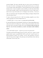
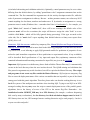
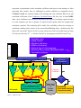
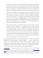
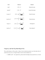
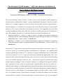
The Stochastic QSAR Sampler – SQS: Introduction, Installation &
User's Guide of the Demo Version
Dragos Horvath, [email protected]
Laboratoire d'InfoChimie, UMR 7177 CNRS – Université de Strasbourg
The herein described version of SQS is a demo version of the Stochastic QSAR (Quantitative
Structure-Activity Relationships) Sampler, a genetic algorithm-based descriptor selection and model
mining tool. It supports aggressive search for linear and non-linear equations (approximating a
molecular property as a function of its descriptors) that can be derived on hand of a given QSAR
training set. The current version allows for training sets of up to 550 compounds, with up to 2000
associated candidate descriptors (the actual code has been successfully run with up to 2500 molecules
and >7000 candidate descriptors). For a detailed technical discussion of this approach, see:
1. Horvath, D., Bonachera, F., Solov'ev, V., Gaudin, C, Varnek, A., Stochastic versus Stepwise Strategies for
Quantitative Structure-Activity Relationship Generation-How Much Effort May the Mining for Successful
QSAR Models Take?, J. Chem. Inf. Mod., 47, 927-939 (2007)
2. Bonachera, F.; Horvath, D., Fuzzy Tricentric Pharmacophore Fingerprints. 2. Application of Topological
Fuzzy Pharmacophore Triplets in Quantitative Structure-Activity Relationships. J. Chem. Inf. Model., 48,
409-425 (2008)
Theoretically, 2N ways to select a subset out of N descriptors exist (in SQS, seven options – ignore, use
as such, or use one of 5 predefined non-linear transformations of a descriptor – are considered, thus
raising the problem space volume to 7N). A minority of descriptor combinations lead to useful models
at all, but a "minority" out of 72000 may still represent an astronomically high number. SQS is not
expected to find all the models that make sense, but a representative sample thereof. Note that finding
one or a few QSAR equations is often very easy – some stepwise regression algorithm may readily
produce impressive training R2 values in a matter of minutes on a workstation. The aggressive problem
space exploration by SQS, based on repeated genetic algorithm-based runs that are piloted by a
controller (also in charge of steadily optimizing the operational parameters of the Darwinian process),
may take days to month to complete on a multi-CPU workstation, depending on problem complexity.
The gain, however, is the obtention of a representative sample of possible models – many of which
may seem redundant in terms of their behavior with respect to training and validation sets, but display
radically different "opinions" concerning predictions of external molecules. The size and apparent
redundancy of the pool of retrieved models is a measure of the intrinsic information content of the data
set. Ideally, the "perfect" training set should leave no room for ambiguity and allow only one
explaining model – the mechanistically relevant one. In real life, however, the training set may conceal
many fortuite, but physically meaningless correlations of different molecular descriptors. Example: in a
training set containing tricyclic antidepressants (actives) and diverse inactives (decoys), it may well
happen that, by pure chance, the aromatic tricyclic system specific to antidepressants will never be
represented among the decoys. Models may conclude that the presence of such a system is a sufficient
condition to be antidepressant – at least that's what the training set suggests. However, the tricyclic
pattern is not the only specific signature that distinguishes antidepressants from decoys – the existence
of an aromatic system connected to a protonable amine is another. This latter GPCR-specific
pharmacophore is mechanistically more relevant a discriminator between antidepressants and decoys –
but, however, not necessarily the statistically optimal discriminator. If fitting a single model, the
outcome may be either the one based on the "tricyclic", or the "aromatic-charge"-based equation –
getting the one or the other is a matter of sheer luck, for they are "indiscernable", i.e. equally well
performing with respect to the training and (therewith related) validation sets. With SQS, there are
good chances to see both being enumerated, offering a series of important a posteriori advantages.
When predicting the antidepressant potential of external compounds, a single model returns a "trust-itor-leave-it" single result. Using multiple SQS approaches, and let each make an independent estimation
of the likeness to be an antidepressant, allows not only to calculate the average of the predictions as a
robust consensus score, but also to analyse the spread of the "opinions" of models with respect to a
molecule. Challenged, for example, to predict the lack of antidepressant effect of inactives containing
large tricyclic aromatic systems, but no cation, the user disposing of a single model may either be
always right (if, by chance, his model is the "aromatic-cation" equation), or always wrong. Note that,
although the single model may use some explicit applicability domain (AD) check, it is highly unlikely
that tricyclics without cationic group be considered outside the AD. By contrast, SQS 1 users will notice
that certain models strongly disagree with respect to the prediction of these compounds. Even though
unable to tell the correct model apart from the artifact (until new experimental data is brought in to lift
the ambiguity), this signals that what had been learned from training set data cannot be extrapolated to
the newly seen molecules. The coherence of predictions from multiple SQS models is an extremely
strong, implicit definition of the applicability domain of the approach: compounds with diverging
predictions are clearly beyond the scope of the approach.
1 SQS models do not, to date, include any explicit applicability domain definitions, but they will in a future release.
Installation Instructions
Install SQS on a multiprocessor Linux workstation, locally or on an NFS-shared disk partition it has
access to. Please make sure that the workstation has at least one local file system with enough free
space for SQS calculations (several GB, depending on the data set size and planned calculations). Be
aware that, although the soft may be safely installed on a network file system (NFS), it has to be run
from a directory of a local disk. Also, make sure your machine has GNU awk (gawk) installed (other
versions of the line interpreter awk might well work, but were not tested).
After ensuring that the machine has enough local disk space for calculations, check the machine type
by entering:
> uname -m
at the Linux shell prompter. If the return is either "x86_64" or "i686" or any other version being
compatible to these two (i.e. other "ix86" using 32-bit libraries), you may proceed with installation.
Otherwise, please contact [email protected] – we might be able to create executables for
different Linux machines as well.
Download SQSdemo.tar and unpack in the HOME DIRECTORY OF A USER RUNNING TCSH AS
DEFAULT SHELL. This creates the SQSdemo directory containing:
scripts
# Directory with scripts and executables
setup
# Directory with control parameter files
data_samples # Directory with a test data sample
cshrc_setups # File to append to your .cshrc
•
The soft might run even in a sh/ksh environment, but was never tested out. It is safer to create a
new user under tcsh, if you personally favor a different kind of shell.
•
You must not necessarily install in the $HOME, but then please edit the lines in cshrc_setups
accordingly:
setenv SCRIPT_DIR $HOME/SQSdemo/scripts
setenv SETUP_DIR $HOME/SQSdemo/setup
setenv TOOLDIR $HOME/SQSdemo/scripts
to point to the new location of the scripts directory.
•
Next, append cshrc_setups to your $HOME/.cshrc and refresh your environment by typing
source $HOME/.cshrc. Note that one of these lines resets the LANG variable to en-US
(American English). The reason is that SQS scripts use (g)awk to process and reformat text
files, and awk is sensitive to the language setup of the parent shell (if yours is set to French,
awk will consider commas rather than dots as a decimal separator and create havoc throughout
the data structures – but never complain or crash: most likely you would witness absurd crashes
of the Fortran executables, which are much less forgiving when it comes to format errors). I
admit I'm not an expert of the subtle issue of awk language context sensitivity – there may be
other ways to make these scripts work properly without changing you language settings, but this
is the only solutions I found.
•
If `uname -m`does not return "x86_64" or "i686", but something compatible to one of these
options, (supposedly x86_64 for the example below), do:
> cd $SCRIPT_DIR; ln -s x86_64 `uname -m` (warning: BACK QUOTES HERE)
•
Be aware that SQS operates in the background, with parent tcsh scripts starting child processes,
which at their turn fire off a child process – until one of these meets termination criteria. Each
such script reads the environment variables from its parent. Therefore, make sure that your
SQS user's .cshrc file does not include any recursive environment variable definitions,
such as:
> setenv PATH $PATH\:/mypath1
# Append my special dirs to the global PATH
The problem would be that the starting script sees a $PATH=<global_path>:/mypath1, its child
appends another /mypath1, its grandchild has $PATH=<global_path>:/mypath1:/mypath1 etc.
Having repetitions in $PATH is not a problem – however, many generations of successive
scripts will cause the sheer lengths of the path string exceed specifications: SQS would stop
with an obscure "Word too long" error.
User's Guide
This is a powerful QSAR building tool, although the current demo version is restricted to training sets
of up to 500 molecules and 2000 descriptor candidates (2500 and 8000, respectively, in the unrestricted
code). It is however not meant for non-expert use. If you do not feel at home in a Unix shell, you may
not be pleased to learn that there is no way to avoid the command line level in order to operate SQS, to
monitor its progress and to detect and understand potential crashes. Depending on the complexity of the
QSAR problem, SQS may run for several weeks without any human intervention. The robustness of the
key executable performing the Darwinian search for properly cross-validating equations is guaranteed –
it has been extensively and smoothly used by us and our collaborators on various (including massively
parallel) Linux workstations and clusters, with hundreds of QSAR data sets ranging from tens to
thousands of molecules. SQS is an elaborate strategy, successively starting parallel deployments of this
executable on multiple "islands", and waiting for their completion in order to analyze the locally found
models and start again, with fine-tuned operational parameters. It is therefore sensitive to issues such as
disk response times (see the repeated warnings against use of NFS-mounted working directories!) or
scheduling conflicts. The latter are problems well-known to users of massively parallel systems, but
typical workstation users may perceive such crashes as completely obscure, random breakdowns.
Fortunately, they are very rare: in the quite unlikely, but not impossible event having two executables
on different "islands" terminating simultaneously, both try to start the master script at the same time –
whereas only one copy of the latter may be active. A master script instance is "instructed" to terminate
if it detects that another one executes – therefore, there is the risk to see both stopping simultaneously.
Manual restarting is required in such cases.
Getting Started
After changing to the working directory – within the local file system of the multiprocessor machine:
> cd local_working_directory
SQS is invoked using the command:
> $SCRIPT_DIR/QSAR_driver.csh act-desc.regdat [paramNameA=valueA paramNameB=valueB ..]
where act-desc.regdat contains the entire activity-descriptor matrix available for QSAR model building
(it includes both training and validation molecules). Optionally, control parameters may be set to values
differing from the default choices, by adding "paramName=value" assignment statements later on the
command line. The first command line argument must be the activity-descriptor matrix file, while the
order of parameter reassignment is arbitrary. Beware – neither parameter names, not values may NOT
contain anything else but letters, numbers and underscores. If, by mistake, an assignment to a wrong
parameter name is made (Windows fans – remember that Unix is CaseSensitive!) - for example, you
typed "Mode=both" instead of "mode=both", there will be no warnings: the default value of the
parameter mode will not be overwritten (the script will however assign the value "both" to a new
variable called Mode... which will be fully ignored during processing). If the typo occurred on the
value side, like in "mode=boht" expect anything from default behavior to funny error reports from
QSAR_driver.csh!
Parameters, SQS data structure with its key temporary files, Manual (Re)Start and Progress Monitoring
and SQS results will be described in more detail in the following paragraphs. Last but not least, the use
of predictor.awk, a tool allowing to apply SQS-generated models for prediction of properties of new
molecules (and immediate comparison of these predictions to experimental values, if any avaialable)
will be described. Brief specifications of key input and output files (explanatory comments of the
contained information and formatting constraints for input files) are given in the Appendix.
Important: SQS operates in a subdirectory (hence forth called the "Master Directory") it automatically
creates in the local directory where the user invokes the tool. The QSAR training and validation data
files passed as arguments may reside elsewhere, but will be copied to the Master Directory. The scripts
and programs do not create any files outside the Master Directory. SQS scripts use temporary flag
files to assess the deployment status of the various executables that run in parallel, as part of the island
strategy used with this genetic algorithm. Therefore, please make sure that the working directory is on a
local file system of the multiprocessor machine when invoking SQS. Trying to run SQS in an NFSmanaged working directory may cause the script to commit deployment errors of the parallel genetic
algorithms, due to the latency of access of the CPU to the remote flag files. Remember – the
installation location $SCRIPT_DIR may be a NFS directory (for example, a software dispensing
disk seen by many workstations), but the directory in which calculations happen must be local. If
NFS latency times are low, NFS-managed remote working directories might work properly – but do it
at your own risks and perils!
Control Parameters of the SQS Driver
Control parameters are needed to specify how to prepare the input data for QSAR building and
validation. The five controls (named in parentheses) concern
(a: vset) the definition of training and validation subsets within the activity-descriptor matrix,
(b: mode, avgfile) the choice of the non-linearity policy of SQS (allowing or denying the
mining for non-linear models, and specifications) and
(c: start, repeat) miscellaneous controls, such as the automatic simulation start toggle and
simulation "cloning" (repeating SQS data mining simulations on hand of a same data set, under
identical conditions, in order to assess the reproducibility of results of this highly stochastic approach).
(a) The vset parameter defines splitting of the input activity-descriptor file into the Learning Set (Lset)
and a Validation Set (Vset) serving to challenge the Lset-trained models. This parameter can be either
set to "auto" (default value) or to a data file enumerating the validation set molecules. By default
(vset=auto), the method proceeds with a five-fold external validation scenario: the initial activitydescriptor file is automatically broken down into 5 random parts. Five independent SQS runs are being
prepared, each based on four of the fifths of the data for training, and the remaining fifth (each time a
different one, of course) kept aside for validation. Each molecule will therefore be part of the validation
set in exactly one of the five considered scenarios. The five runs are, of course, fully independent and,
if the initial set happens to contain small (<<1/5 of total size) specific compound subfamilies risking to
be simultaneously singled out for validation, both the nature of retrieved models and their validation
propensities may strongly fluctuate from one run to the other. Comparable results, irrespectively of the
splitting scheme, is a first indicator of satisfactory training set quality. In any case, artefactual
relationships that emerge as a consequence of specific Lset/Vset split-ups are being seriously downplayed by this approach (at the end, a consensus prediction based on models having witnessed different
Lset/Vset definitions is much more robust than one based on models emerging from a rigid
training/validation scheme). However, this option requires a five-fold increase in computer effort
compared to a standard single Lset/Vset split that can be implemented by using the
vset=validation_set_list_file.vset directive. Suppose that, for benchmarking purposes, you wish to use
the same training/validation scheme as employed by previous workers on your data set. Knowing
which molecules are to be spared for validation allows you to enter the list of their comma-separated
sequence numbers in validation_set_list_file.vset. In typing:
> echo "1,6,7,12,22,29,34,43,59,62" > validation_set_list_file.vset
you generate a validation subset containing molecules nr. 1,6,7,12,22,29,34,43,59,62 (these numbers
refer to the initial compound list that was used to generate the activity-descriptor matrix provided as
input. Note that these are not line numbers of the activity-descriptor matrix, which mandatorily
includes a first column label line: the herein specified molecule list would trigger selection of lines nr.
2,7,8,13,... etc. from the activity-descriptor matrix). You cannot use any molecular ID fields in .vset
files – if your validation set make-up originally consists of a list of say CAS numbers, you need to
convert in into a list of sequence numbers by locating the position of each compound matching one of
your CAS IDs in the list of compounds that produced the activity-descriptor matrix).
(b). The mode parameter controls the non-linearity policy of the planned SQS run. Setting mode=lin on
the command line will restrain the search of models to the realm of linear equations. By, default,
however mode=both, e.g. for each considered Lset/Vset split, two different SQS mining attempts will
be performed – one allowing for non-linear transformation functions, the second one not. Setting mode
to anything else but lin or both will be interpreted as a desire to generate non-linear models only. If
non-linear modeling is enabled, SQS must be told how to choose, for each of the considered
descriptors, the critical point and width parameters for the predefined transformation functions
(Gaussians & Sigmoids). These functions require to define, for each descriptor a critical point
(maximum, for Gaussians; inflexion point for Sigmoids) corresponding to some "average" value of the
descriptor – in the sense that, throughout the data set, molecules with descriptors both above, around &
below this critical point must be represented in order to have a meaningful non-linear transformation.
The associated width factor is typically a measure of descriptor variance. Setting the parameter
avgfile=local (which is also the default behavior) will automatically extract associated critical
points=descriptor average values and width=descriptor variances from the provided activity-descriptor
matrix. Gaussians will thus peak and Sigmoids toggle at the center of the descriptor space covered by
the input examples (note that the averages/variances are taken over the entire input set and are thus not
dependent on the Learning/Validation splitting schemes). Alternatively, you may enter a file name
avgfile=AVG_VAR.dat specifying other values for these parameters – for example, averages and
variances calculated with respect to the Universe of drug-like molecules rather than locally. You may
of course enter any values: if they do not make sense (null or negative parameter for the variance, for
example), the concerned descriptor will not be considered for non-linear transformations but may still
participate as a linear term. The file (three tab/space-separated columns: 1 – descriptor name, as listed
in the header of the activity-descriptor matrix, 2 – critical point parameter or "average", 3 – width
parameter or "variance") needs not list all the candidate descriptors available in the activity-descriptor
matrix: the absent ones will by default be reserved for linear usage only.
(c) Automatic simulation start: by default, QSAR_driver.csh prepares all the data structures needed for
model building under the various premises (learning/validation setups and non-linearity policies
enumerated above) and then stops, allowing the user to control its output and then manually start model
building. However, this default "safe" behavior can be overridden by specifying start=go on the
command line, when the procedure automatically starts model building after having generated the data
structures (it won't even thank you for trusting its data preparation skills).
Repeating simulations: by default, a single model building simulation is performed for each considered
learning/validation setup and non-linearity policy combination. However, remembering that the first
"S" in SQS stands for "stochastic", you might want to repeat the simulations, in order to check whether
the same equations will be rediscovered (probably not!) or, at least, whether repeated runs lead to sets
of models displaying comparable training and validation performance (most likely yes, please consult
the discussion on reproducibility in the cited SQS publication). Setting the control parameter repeat=n,
with n>0 will automatically create n additional clones of a simulation subdirectory (therefore, the
computer effort will scale as n+1). By default, repeat=0.
Note: unlike the herein distributed demo version, the actual QSAR_driver.csh may be called with a
SMILES-activity file (tab/space separated 2-column file having the molecule SMILES in column one
and the activity score in column 2) instead of the activity-descriptor matrix. It will produce an activitydescriptor matrix including ISIDA fragment counts, fuzzy pharmacophore triplets and ChemAxon
descriptors (logP/logD, BCUT terms and pharmacophore pairs). Additional parameters can be provided
to control this process: triplets = <pharmacophore triplet version: default FPT1>, fragtype =
<fragmentation scheme, default 3, i.e. atom & bond sequences>, shortestfrag = <shortest path length
for included fragments, default 3>, longestfrag = <maximal fragment path length, default 6>.
SQS Data & Process Flowchart and Key Temporary Files
The data structures generated by a SQS run will be exemplified on hand of the provided
Acetylcholinesterase data set in $HOME/SQSdemo/data_samples. First, change to a directory in which
calculations are to be hosted (not necessarily the one holding the input data, and remember it has to be
on a local file system of the calculator). Ask SQS to generate the data structures required to build only
linear models, using a one-fold external validation step according to the already provided splitting
scheme:
> cd /local_file_system/workdir
> $SCRIPT_DIR/QSAR_driver.csh $HOME/SQSdemo/data_samples/AChE.regdat mode=lin
vset=$HOME/SQSdemo/data_samples/AChE.vset
Note that calculations will not actually begin – no start=go directive has been added. You will notice
that, at your current location, the SQS Master Directory AChE.QSAR has been created. As you have
guessed, the Master Directory name is obtained by stripping off access path and extension of the
activity-descriptor matrix AChE.regdat and appending .QSAR to it.
Change to the Master Directory and list its contents:
> cd AChE.QSAR/
> ls
AChE.regdat Lset1.regdat Vset1.regdat runL-1.0
Note that the initial AChE.regdat has now been copied to the current directory, and two subsets Lset1
and Vset1.regdat were generated according to the splitting rule in AChE.vset. This file enumerates 37
molecules by their ordinal number in the activity-descriptor matrix AChE.regdat. Therefore, the
validation subset Vset1.regdat contains 38 lines (header/label line + 37 activity-descriptor entries). 74
of the 111 molecules are in Lset1.regdat, ready for training.
The actual SQS run(s) will happen in the Run Directory runL-1.0. For this time, there is only one Run
Directory because a single splitting scheme has been employed in conjunction to a single non-linearity
policy, and no repeated runs were demanded. A Run Directory name is automatically generated under
the form run<Non-linearity policy code: L or N>-<Lset/Vset splitting scheme number>.<repeatcount>. In order to exemplify a situation with multiple run directories are generated, return to the
initial directory, remove the Master Directory AChe.QSAR and ask QSAR_driver.csh to prepare a fullblown 5-fold external validation scheme (vset=auto – no need to type that, it's the default) , mining for
both linear and non-linear approaches (mode=both – default as well) and using the provided
AChE.avg_rms file to specify the critical point and width parameters for the non-linear transformations
(avgfile=$HOME/SQSdemo/data_samples/AChE.avg_rms). Also ask for one repeated run of each
setup:
> cd ..
> rm -r AChE.QSAR
> $SCRIPT_DIR/QSAR_driver.csh $HOME/SQSdemo/data_samples/AChE.regdat repeat=1
avgfile=$HOME/SQSdemo/data_samples/AChE.avg_rms
The new Master Directory will now contain 2x5x2=20 Run Directories named run[L,N]-[1-5].[0,1],
where run[L,N]-[1-5].0 and run[L,N]-[1-5].1 are strictly identical "clones" of a same setup (although
they will differ in terms of the contained results, once the stochastic process is started).
A linear Run Directory contains the following key files:
ACT.regdat -> ../AChE.regdat
# link to the entire activity-descriptor matrix
Lset.regdat
# learning set – copy of ../Lset1.regdat, splitting scheme #1
Vset.regdat
# validation set – copy of ../Vset1.regdat, splitting scheme #1
expt_high.gen, expt_low.gen
# upper/lower bound of activity range, extracted from ACT.regdat
strict_linear.gen
# flag file telling the sampler to stick to linear models
todo.flag
# temporary flag file while directory awaits being processed
Note that, within each Run Directory the learning/validation sets are always called Lset.regdat and
Vset.regdat. However, their contents depends on the current splitting schemes – they are respective
copies of Lsetn.regdat and Vsetn.regdat from the Master Directory, where n is the current splitting
scheme number found in the Run Directory name.
By contrast to a linear run, non-linear Run Directories differ by the fact that strict_linear.gen is being
replaced by AVG_RMS.dat (a link to the file residing in the Master Directory and which, in this case, is
nothing but a copy of the specified $HOME/SQSdemo/data_samples/AChE.avg_rms).
Manually (Re)Starting the SQS process.
Unless called with the start=go directive, QSAR_driver.csh stops after having created the required Run
Directories, allowing the user to inspect the consistency of the created data structures. After having
done so, change directory into either one of the Run Directories and enter:
> $SCRIPT_DIR/autoreg.csh new
If SQS has crashed (in our hands, this rarely happened due to scheduling conflicts), locate the latest
Run Directory in which it was operating, cd there and enter:
> rm autoreg.scriptactive
> $SCRIPT_DIR/autoreg.csh cont
SQS Progress Monitoring
Upon (re)start the SQS deployment procedure, soon enough a number of "islands" will be created in
the Run Directory. They are named cont_localhostn, "cont" standing for "continent" rather than
"island" (both terms are interchangeably used in conjunction with genetic algorithms). Therein,
cont_localhost*/status files report the progress of the Darwinian evolution. The number of continents n
is one of the operational parameters to be fine-tuned by the meta-optimization loop. Other such
operational parameters include the population size, the mutation frequency, etc. In the Run Directory,
selected parameter values are written out into control files having the extension .gen: try head -1 *.gen
to obtain a full list of the parameters and their values chosen for the current Model Building Stage. At
given "Model Building Stage (MBS)" (graphically corresponding to the yellow rectangle in the
Flowchart), the content of the *.gen files is invariant – these are picked from a master file
$SETUP_DIR/reg_parameters.lst, listing the parameter name, the number of choices allowed and their
list. Which of the choices will be picked is determined by the meta-chromosome associated to this
MBS: it can be found in the file current_setup. The meta-optimizer first generates a set of 10 metachromosomes in setup_waiting_list, then takes these sequentially into current_setup and performs the
associated MBS. An MBS consists in a three-fold repeat of the island model deployment, according to
current_setup. After completion, the scripts calculate:
•
an associated list of locally optimal model chormosomes (all_solutionsMBS, where MBS is the
current model building stage number – the "base of diverse models" in the Flowchart),
•
the success score of the MBS (the "meta-fitness" µ-Fitness, to be written out, next to the
current_setup that has produced it, into a file called setups_best).
•
a directory of the best models to date, ModelsMBS. This will enumerate the best models found
from the beginning of a simulation until the currently completed MBS, and not only models
found during the latest MBS. It therefore corresponds to the current instance of the "Global
Base of Diverse Models" in the Flowchart. The directory contains individual equation files
modelM.eq, numbered 1 through M, and consensus model files consXX.eq, average equations
of the modelM.eq, where XX stands for the empirical temperature factor if "Boltzmann"
averaging2 is used, or XX="R2" if the participation of individual models into the consensus
2 The participation of an equation to the consensus will be proportional to exp(XX*R2)
expression is proportional to their correlation coefficient with respect to the training set. After
generating these models, they are challenged to predict validation set compound activity.
Validation results are reported, together with training and cross-validation RMS errors and
correlation coefficients, in the Temporary Top Model Report file final_stats in ModelsMBS.
Note – these validation scores are never exploited by the SQS run, but simply reported in order
to let the impatient user have a glimpse of expected model quality before the lengthy SQS
simulation completes. The numbering M of model files modelM.eq reflects the training set
performance ranking, and is relative to the current Model Building Stage – the historically first
discovered "top model" Models1/model1.eq may remain one of the best models known at stage
#29, but now rank only 23th – i.e. Models1/model1.eq also appears as Models29/model23.eq
Molecule
…
pIC50
D1
D2
D3
…
DN
4.2
0
0
73
…
39
8.7
18
0
0
…
44
5.8
43
0
5
…
0
…
…
…
…
…
…
4.0
0
0
9
…
0
• Population size
• Island number
• Migration frequency
• Mutation frequency
• Maximal Age of chromosomes
• Selection/Size controls (MAXMAXVARS, π, pOcc)
• Termination Criteria
MetaMeta-optimizer defines parameter setup
Run
1
Run
2
…
Run
n
MetaMeta-optimizer picks
next set of
configurations
« Taboos »
« Tradition »
News
??
Postprocessing…
3-fold repeat
Figure 1: SQS Flowchart
µ-Fitness!!
Base of diverse models
[sampled at current setup]
yes
Global Base
of
Diverse
Models
no
•Scrambling
•Final model selection
•Consensus models
SQS Completion of a Current Study in a Run Directory
As SQS progresses, all the operational parameterization schemes from setup_waiting_list will transit
into current_setup and terminate in setups_best, associated to their sampling success score. As soon as
setups_best includes all the lines from setup_waiting_list, a meta-generation µg of the meta-optimizer
has elapsed. A population.µg file will be created, regrouping the 10 fittest setups encountered so far (in
setups_best or in older population files). If population.µg is identical to its "grandparent" (at µg-2
generations), i.e. the two lastest setups_best files did not contain any better sampling success (note –
better means "more negative") then mining for models is completed: SQS switches to scrambling tests.
Using the 10 operational parameter setups that maximized sampling success for the given problem,
SQS tries to fit artefactual models after randomly associating activity values from Lset.regdat to
molecular descriptor values. Note that scrambling implies a full-blown descriptor selection and model
building attempt, not a simple testing whether already selected subsets of descriptors from ancient
successful models may apply to the scrambled training set. There are 10 additional attempted Model
Building Stages, which do however not generate any ModelsMBS and the artefactual models are not
explicitly written out. However, the distribution of the fitness values of real and artefactual (scrambled)
models are plotted into two histogram files real.hist and scrambled.hist respectively. These are, in
principle, (x,y) pair files representing, on Y, the fraction of models having a fitness score of about X –
however, in order to facilitate visualization, they actually contain the (x,y) values of a broken line
explicitly drawing the histogram boxes. The boxes in real.hist are furthermore offset by one X tick with
respect to scrambled.hist, so that peaks associated to a same X value will not overlap. You may load
and visualize these curves with any plotting program – for gnuplot, for example, use:
gnuplot> set style data lines; plot "real.hist" title "Real","scrambled.hist" title "Scrambled"
Note that the X axis represents the actual brute fitness score of the genetic algorithm, which is
conceived as a minimizer. Therefore, these scores are the negative value of the penalized crossvalidated correlation coefficient – high peaks at negative X values (-1 being the absolute optimum)
mean many nicely cross-validating models. The real model distribution should peak at the left hand of
the plot, and ideally never overlap with the one of the scrambling-induced models.
At this point, SQS processing of the current Run Directory is completed, and the pilot script marks this
chapter as closed by removing the flag file todo.flag, then descends to the parent (Master Directory) to
search whether there are other Run Directories still awaiting to be processed (containing todo.flag).
Therefore, all the Run Directories will be visited, one by one. To know which Run Directory is
currently being processed, go to the Master directory and list by access time: ls -lt| grep run to see it
appear at the top of the list.
Final SQS Results
After going through all the Run Directories, the SQS script completes by creating, in the Master
Directory, a single list of all the models encountered: models.lst. Its format is the same as the one of
the Temporary Top Model Report files final_stats. However, model names are prefaced by the Run
Directory in which they were built. Models are listed only once in models.lst, although they may
appear under different names in several temporary reports. Note that in principle, if you have
several available computers that may run SQS, you do not have to wait for Run Directories to be
processed one after the other, but move them to different local file systems of the available machines
according to a rule of you choice (if, for example, you'll use two computers move all the linear Run
Directories to the second machine: mv runL-* /newmachine/tempQSAR/ and process the non-linears on
the current. You may also cp instead of mv, but then do not forget to clean runL-*/todo.flag so that the
local SQS script processes only the runN directories). Then, on each machine, start SQS manually from
one of the Run Directories – as far as they were all moved into a common parent directory, SQS will
"jump" from one to the other without problem. After completion, bring the displaced directories,
including their results, back to the departure point and please note that, in this scenario, models.lst has
to be rebuilt manually (find & use the appropriate command line in $SCRIPT_DIR/autoreg.csh) after
reuniting the Run Directories.
Predicting Compound Properties with SQS models.
SQS models learned, on hand of training examples, to estimate a molecular property in terms of some
important descriptors. They may now be used to predict this property for new compounds, provided
that the key descriptor values of these molecules are given. The tool applying a specified SQS model to
calculate a property estimator on the basis of input descriptors isa GNU awk (gawk) program,
$SCRIPT_DIR/predict.awk. This script reads a tab/space separated descriptor file, with the first line
containing descriptor names – like the activity-descriptor matrix, except that now, of course, the
presence of a property column is no longer mandatory. The second key parameter, to be passed to
gawk as a variable (-v option) called model is, of course, the .eq file of the model to be applied.
Example:
> cd prediction_dir/
> gawk -f $SCRIPT_DIR/predict.awk -v model=..path../RunDir/Models8/model13.eq Mols.dat
The predictions (by default, a two-column output: descriptor line number, followed by predicted
values) will be printed on standard output, which is not very useful when dealing with many molecules:
append "> output.pred" to the commands in order to redirect everything into a file. With non-linear
models, gawk may sometimes complain that the argument of the exponential function in Gaussians or
Sigmoids is "out of range" – for descriptor values far away from the critical point, considering the
width parameters. Beyond a certain value of x, exp(x) in gawk will return the string "inf", while for
very negative x values, it will correctly return 0. However, gawk properly returns 0 for 1/(1+"inf") in
case of positive argument overflow in sigmoids, so, at the end, this mathematical peculiarity of gawk
has no consequence, error messages notwithstanding (those, incidentally, are output on standard error,
so redirection > output.pred will not collect them into the result file). Remains the philosophical
question whether the model is still applicable to compounds with descriptor values so far away from
the critical point of the non-linear transformations (recall the brief discussion in Introduction).
Other important aspects concerning predict.awk:
•
As you may have well guessed, the request of having descriptor names as column titles in
Mols.dat signifies that it is matching column headers against the list of descriptors entered in
the .eq file. Make sure that these are spelled strictly identically (CaseSensitivity included).
•
As a consequence of using column titles, it does not matter in what order the descriptor columns
occur in Mols.dat, nor whether this file also contains additional columns.
•
If, however, the .eq file expects a descriptor not found in Mols.dat, the program will, by default,
assume that a descriptor value of 0 has been input, and continue calculations without issuing a
warning. This "assume null if not listed" hypothesis makes sense in as far you are working with
fragment or pharmacophore element counts as descriptors: the molecules were submitted to the
fragmentor or pharmacophore pattern detector, and since the fragment/pattern did not show up
in Mols.dat it's certainly because it is not populated in either of the compounds to be predicted.
However, it does not make sense for whole-molecule descriptors: if forgotten to provide the
Kier-and-Hall indices, assuming they all equal zero will not fix the blunder. Please note that
predict.awk will not remind you to provide the missing column, unless the special variable
missing_value is not set to 999 (use -v missing_value=999 in the gawk command line). Doing
this will cause the program to halt upon failing to find a required descriptor among the column
labels of Mols.dat. Setting missing_value to anything else but 999 will prompt predict.awk to
use that value for any missing descriptor, rather than zero.
•
If Mols.dat actually contains an activity column, predict.awk may automatically compare the
calculated values to the existing ones (if -v act_label=title_of_activity_column is explicitly
added to the command line, in order to let the predictor know that Mols.dat contains activities,
or if the column in question is labeled "ACT" and is therefore recognized as such by default).
The predictor output will then consist of three columns: current number, experimental value
from Mols.dat and predicted value. At the end, the predictor will list the results of various
correlation tests between experimental and predicted values: these lines are "outcommented" –
they all start with "#". If you wish to generate an (experimental, predicted) plot from the output
of predict.awk, do not forget to remove these lines using fgrep -v #.
The following example shows how you can use multiple SQS models – specifically, only the models
simultaneously having high training and validation propensities – to let each model predict the
properties of new compounds and therefore assign any new molecule into a predefined activity
category. At the end, the result table will show, for each molecule, the number of models that assigned
the molecule into each activity category. Selected, of course, will be compounds for which a majority
of models "agreed" to place them into the category of interest for the experimentalist.
1. Preliminaries: First, generate the descriptor file of the molecules you want to subject to virtual
screening, Mols.dat. Copy it to the Master Directory of the QSAR models, next to the Final Top Model
report, models.lst. Also, you might want to associate the predictions to some molecular identifiers:
supposed you have a column file of molecular identifiers corresponding to Mols.dat, copy it to the
Master Directory as well, and name it "results.out". This file will serve as a template for predicted
category count output, as shown later. Note: results.out, unlike Mols.dat, should contain no title line
2. Model selection: pick the models you wish to use for predictions out of models.lst. Remember that
models.lst enumerates equations that, historically (during the evolution) appeared as the most
interesting in terms of training set cross-validated correlation coefficient. It may thus contain equations
with relatively poor training R2 (primitive "animals" that were fittest at early ages of "life") and,
notably, many models with poor validation propensities (overfitted equations failing to apply to the
validation set). Pick, for example, only models having R2T>0.8 (R2T being the column nr. 6 in
models.lst, that gives "$6" in gawk language) and also having the validation set RMS errors (RMSV,
"$5") of comparable magnitudes (less than 20% increase) to the training set RMS errors (RMST, "$3").
Do not forget to strip the title line of models.lst (NR>1) off, and print out selected models ("$1") into
used_models.lst:
> gawk 'NR>1 && $6>0.8 && $5<=1.2*$3 {print $1}' models.lst > used_models.lst
Note that the empirical thresholds must be adapted to your current situation: if no model trains at
R2>0.8, revise the "$6" constraint accordingly. Defining "not overfitted" can be simply achieved by
setting a minimum threshold for the validation correlation score R2V ("$9>0.6", for example). Also,
models.lst also lists local consensus equations that were produced during evolution history (in fact, the
reason for selecting with respect to R2T instead of the cross-validated coefficient R2XV is that the
latter is not defined for consensus models, and set to 0). If you do not wish to maintain these consensus
terms in your selection (arguing that the parent equations at their origin will be part of it anyway, and
hence be given the occasion to participate in consensus scoring directly), use a R2XV-related threshold
"$7>0.7" instead. Since in models.lst equation files are already prefixed with their relative access path
with respect to the Master Directory, used_models.lst should now be a one-column file featuring entries
like "runN-1.0/Models7/model18.eq"
3. Decide upon the prediction categories you wish to consider. Supposing, for example, that the
predicted property is a pIC50 value, a first category regrouping anything below 4 would represent
"milimolar" compounds, 4≤predicted pIC50<5 stands for category 2 (100 µM), etc..., up to category 7
(nanomolars) with 9≤predicted pIC50. Starting from the predicted value p, the category index C could
therefore be written as C=max[1,min(7,int(p)-2)]. Therefore, if we capture the standard output of
predict.awk, where p can be found in column nr. 2, the following pipe would, for any given model,
return a column output listing the category assigned to each molecule by that model:
> gawk -f $SCRIPT_DIR/predict.awk -v model=[some_model_from_used_models.lst] Mols.dat| gawk
'$0!~"#" {c=int($2)-2; if (c>7) c=7;if (c<1) c=1;print c}'
Above, $0!~"#" is used to force ignoring any outcommented lines output by predict.awk.
4. Actual prediction can be performed in the C-shell, by means of a foreach loop browsing through the
models recuperated form used_models.lst, using the backquote syntax. For each model, a category
column would be output by the above-mentioned pipe of commands. However, since it is cumbersome
to generate as many temporary one-column result files as there are models in used_models.lst, the
utility gawk script insertcol.awk will be used to capture category columns at the output of the pipe and
paste them as left-most new column to results.out. This contains, as a first column, molecular ID values
and, after completion of the foreach loop below, will be updated with as many additional columns as
there were selected models, the column i+1 enumerating the categories into which model i (in the order
given in used_models.lst) would have classified the molecules:
> foreach model_file (`cat used_models.lst`)
foreach? gawk -f $SCRIPT_DIR/predict.awk -v model=$model_file Mols.dat| gawk '$0!~"#"
{c=int($2)-2; if (c>7) c=7;if (c<1) c=1;print c}'| gawk -f $SCRIPT_DIR/insertcol.awk results.out
foreach? end
Lines (molecules) containing a maximum of values of 6 and 7, but not a single 3 or 4 are definitely the
most likely candidates for selection, (a majority of models agrees to rank them among the very actives,
but even though, according to other models they may be only mildly active, none ever considers them
inactive). The analysis of the spread of "votes" of each model for a molecule is more informative than
"plain" consensus modeling, which simply returns an average of all individual predictions. How to
gawk out the subset of nanomolar blockbuster drugs from results.out is left as an exercise to the reader,
who must have been quite a Linux fan in order to keep on reading until this point.
Appendix: Content, Meaning and Format of Key Files
The SQSdemo/data_samples subdirectory contains input file examples of the acetylcholinesterase
inhibitor data set as used in the second publication cited in the introduction.
Activity-Descriptor Matrix
This is a plain tab-or-space-separated text file with a constant number of columns, featuring first a title
line with all column headers, followed by data lines (one per considered molecule) in which the first
entry is an activity score, while remaining columns are molecular descriptors. Except for the title line,
containing ASCII text labels, all the rest must be numeric entries. Note that categorical data are
anyway not supported by SQS, which is a regression engine. However, there is no constraint
whatsoever concerning the numeric format (in as far as you stick to the dot as a decimal separator
rather than a comma) – floats (at arbitrary precisions) and integers may coexist within a same line or
column. The title line must feature exactly as many space-or-tab-separated words as there are numeric
entries in the following lines. The first entry on the title line is the activity column label: please use
ACT as a column header of the first column. Otherwise, the scripts will have troubles in realizing that
an activity data column was actually provided. Warning: descriptor labels must consist of single words
and contain no quotes, spaces, etc. Here are some examples of bad practices in preparing the activitydescriptor matrix:
•
Do not quote words on first line:
"ACT" "logP" "logD"
...
1.0
3.8
0.7
...
1.3
1.8
-0.2
...
•
Do not use spaces in descriptor names: the scripts seek for 4 descriptors("log","P","Randic" and
"Index") but find only 2 values
ACT log P
log D
...
1.0
3.8
0.7
...
1.3
1.8
-0.2
...
•
Quoting will not make the program understand that spaces should be assimilated into descriptor
names
ACT "log P" "log D"
...
1.0
3.8
0.7
...
1.3
1.8
-0.2
...
•
Nice attempt to label the activity by its name, but that will cause confusion: please use ACT
instead of pEC50
pEC50
logP
logD
...
1.0
3.8
0.7
...
1.3
1.8
-0.2
...
For a quick consistency test of your input file, use awk '{print NF}' myfile.regdat| sort| uniq -c. This
command should return two numbers on a single line: the first is the count of lines in myfile.regdat and
the second the number of fields of each line. If the number of fields changes from line to line in
myfile.regdat, you will have multiple returns (nr_of_lines_with_N_fields, N), which means
myfile.regdat is corrupted.
Validation Set Specificator
This file must contain a single line of comma-separated molecule sequence numbers and no spaces,
tabs and other characters – including newlines. If the positions the validation set molecules occupy in
the initial set are available to you under the form of a column file column.lst, you may convert it to the
.vset format using:
> awk '{vstring=vstring","$1} END {sub(",","",vstring);print vstring>"my.vset"}' column.lst
(note that column.lst may contain other columns as well, if the wanted position numbers are not listed
in column one but in some other col_nr, use $col_nr instead of $1)
Otherwise, assuming you start with a two-column file data.ss in which the first corresponds to the
SMILES of the molecules in the submitted data set (in the order of the entries in the associated activitydescriptor matrix), while the second column is a Status variable equaling "L" if the molecule is part of
the learning set, and "V" otherwise, then use:
> awk '{if ($2=="V") vstring=vstring","NR} END {sub(",","",vstring);print vstring>"my.vset"}' dat.ss
Critical Point & Width Specifications for Non-linear Models
Files passed by means of the avgfile parameter are supposed to contain three tab/space-separated
columns:
1 descriptor name, as listed in the header of the activity-descriptor matrix (same restrictions apply),
2 critical point parameter or "average",
3 width parameter or "variance"
The latest two may be given in free float or integer numeric format (use decimal dot, not comma!).
Darwinian Evolution Status Files
This one-line file shows:
•
the current generation,
•
four fitness scores where the three first belong to the most fit, the last to the less fit member of
the current population,
•
the maximal number of variables allowed to enter the equation at this evolutionary stage,
•
the birth date (in generations) of the fittest member ever encountered so far
•
the number of generations elapsed since the last remarkable progress of the fitness of the best
ranked one or two individuals
Equation Files
These .eq files contain all the information pertaining to a predictive model. At first, "comment" lines
starting with "#" contain various parameters, such as statistical performance at training stage (but not at
validation – remember that this file has to be created first, for it contains the model to be validated!).
Upper and lower cutoff settings are not only given for the user's information, but are actually applied,
at prediction stage, to truncate the brute linear combination of descriptors and their non-linear
transformations. Commented lines at the end of the model file offer a detailed listing of predicted
property values for the training set compounds,.
The core description of the predictive equation is contained in the central, uncommented block of lines
(to view only these, use fgrep -v # modelM.eq). These lines enumerate selected descriptor, its chosen
transformation (see below and note that, if a transformation has been applied, its critical point c and
width w parameters are exported in the model file) and the participating coefficient. Unless this section
contains an explicit "Intercept" entry, the free term of the linear combination is assumed zero.
Code
Function
Remark
“none”
T1 ( D ) = D
Identity function
“squared”
T2 ( D ) = D
Squared descriptor
2
“zexp(c:w)”
  D − c  2 
T3 ( D ) = exp− 
 
  w  
Broad Gaussian
“zexp3(c:w)”
  D − c  2 
T4 ( D ) = exp− 3 
 
  w  
Sharp Gaussian
“zsig(c:w)”
“zsig3(c:w)”

 D − c 
T5 ( D ) = 1+ exp 

 w 



T6 ( D ) = 1+ exp 3


−1
D − c 

w 
Flat Sigmoid
−1
Steep Sigmoid
Temporary and Final Top Model Report Files
These multicolumn text files provide a listing of some statistical parameters (see first header line) of
models harvested so far, covering the behavior in the external validation test:
•
1: MODEL_FILE – the equation file, prefixed in the Final Report by the path where it is found
(in Temporary Reports, it is understood that .eq files reside in the same directory as the
temporary report final_stats iself).
•
2: NVARS – number of variables entering the model
•
3: RMST – training set RMS error btw. experimental and predicted properties
•
4: RMSVf – "fitted" ("fudged"??) validation set RMS error, calculated under the assumption
that, for validation molecules it is acceptable to have predicted values strongly differing from
experimental values if there is nevertheless a linear relationship between the two: Yexp=aYpred+b|
. RMSVf then represents the root-mean-squared error between Yexp and this "re-
Validation Set
prediction" Yrepred= aYpred+b. We however strongly discourage the use of this criterion, added
only in order to facilitate comparison to the work of people systematically refitting their
regression line to accommodate validation results. This is, in our opinion, not a good practice
(euphemism for "cheating") – for allowing Yexp=aYpred+b|Validation Set contradicts the fact that, for
training compounds, Yexp=Ypred. So, if a and b differ strongly from 1 and 0 respectively, which is
then the correct equation to be used for prediction – the original Y pred as emerged from training,
or the Yrepred introduced to keep training set happy? If a and b fail to approach 1 and 0, this
simply means that validation failed – if not, then there is no need for a and b, anyway. One may
argue that, if a>0 then the validation set compounds were at least properly ranked by the model:
however, it is arguable to claim validation success on such a weak basis.
•
5: RMSV – actual root-mean-square error between predicted and experimental property values,
without any further concession.
•
6: R2T – training set correlation coefficient
•
7: R2XV – training set leave-a-third-out cross-validation coefficient. Note that this is artificially
set to zero for consensus models, which are built by averaging the equations fitted and crossvalidated with respect to the training set. While their R2T can be easily recalculated a
posteriori, there is no cross-validation stage involved in consensus model building.
•
8: R2Vf – the "fitted" validation correlation coefficient, corresponding to the heavily criticized
RMSVf: better ignore!
•
9: R2V – the proper validation correlation coefficient, reporting the observed RMSV to the
internal variance of the validation set. Please be aware that low (even negative!) R2V values
simply mean that the error between experimental and calculated properties is much larger than
the range covered by the experimental values in the training set. If a model is trained on hand of
inhibitors of nanomolar to milimolar strength, a characteristic inaccuracy of 1 on the pKi scale
would ensure an excellent R2T score. However, if challenged to predict the activity of a set of
nanomolar binders only, having all predictions within 1 log of accuracy (which is an excellent
result) would nevertheless lead to a lousy R2V value because there is virtually no variance of
the property within the validation sets. We here do not follow some author's idea to calculat
R2V by comparing the prediction RMS error RMSV to the experimental variance of properties
of the training set which, in the above example, would have returned an excellent R2V (at same
prediction quality as reflected by RMSV). Therefore, our suggestion is to compare RMSV to
both RMST and to what is practically acceptable in terms of prediction errors for the QSAR to
make sense. If RMSV is acceptable, then the model is acceptable (within the intrinsically
limited guarantees offered by this necessary, but hardly suficient external validation test). If
R2V, however, is not acceptable, then it is not directly the model, but the validation set design
that needs to be questioned. This fragilises model validation anyway, for a low-variance
validation set composed only of actives or – more likely – only of inactives would tell
preciously little about the ability of the model to discriminate between actives and inactives,
even if it got all the actives or all the inactives right!)