Download USER MANUAL - the Open Source Geospatial Laboratory at ETH

 USER MANUAL Version 1.0 22.05.2009 Preface
This documentation was created in May 2009 and represents the state of QGIS mapserver at the time of May 22nd 2009. It is intended to guide first time users through the workflow of publishing and editing a web based map with QGIS mapserver. QGIS mapserver is a cartographically advanced mapserver published under the GPL license. Author: Sandra Zeder, ETH Zurich Table of Contents
Table of Figures 1 Basics iii 2 1.1. Web Mapping 1.1.1 Client‐server architecture 1.1.2 OGC 1.1.3 Web Map Service 1.1.4 Map server 1.1.5 Styled Layer Descriptor 1.2. GIS 1.2.1 Data formats 2 3 3 3 4 5 5 6 2 3 7 8 3.1. 3.2. 3.3. 4 5 What should I know about QGIS Mapserver? Installation of QGIS and QGIS Mapserver Windows Linux Mac OS X Folder Structure of QGIS Mapserver Data Processing in QGIS 5.1. 5.2. 5.3. 5.4. 8 9 10 11 12 Starting QGIS Desktop Version Manage Plugins Shapefile in PostGIS Import Tool Preparation of Data in QGIS 5.4.1 Changing the Coordinate Reference System 5.4.2 Symbolization of Data 5.4.3 Diagram Overlay 5.5. Data Publishing with QGIS Mapserver 5.6. Editing an „admin.sld“ file 5.6.1 Structure 5.6.2 Symbolizers 5.6.3 Filter Encoding 12 12 13 16 16 18 20 21 24 24 25 26 6 27 6.1. 6.2. 6.3. 6.4. 7 7.1. Clients QGIS Open Layers Carto.net Map Bender Examples Polygon Symbolization 7.1.1 Creation of an „admin.sld“ file for Polygons 7.1.2 Adaption of the Dasharray of an Outline Stroke 7.1.3 Creation of a User‐defined Pattern in SVG 7.1.4 Filter Encoding Line Symbolization 7.2. 27 28 29 29 31 32 32 36 36 38 40 i QGIS Mapserver Table of Contents 7.2.1 Creation of an „admin.sld“ file for Lines 7.2.2 Adaption of the Line cap 7.3. Point Symbolization 7.3.1 Creation of an „admin.sld“ file for Points 7.3.2 Adaption to a different Point Symbol 7.3.3 Adaption to a User‐defined Point Symbol 7.4. Text Symbolization 7.5. Diagram Symbolization 7.5.1 Creation of an „admin.sld“ file for Diagrams 7.5.2 Adaption of the Zoom Dependency of Diagram Size 7.6. RasterSymbolization 40 42 43 43 46 47 48 49 49 53 54 8 Index 9 Bibliography 10 Appendix 57 58 60 ii QGIS Mapserver Table of Figures Table of Figures
Figure 1: Map types (Kraak, 2001) Figure 2: Structure of a WMS request Figure 3: Client‐Server‐Architecture Figure 4: Vector data Figure 5: Raster image Figure 6: Download of “qgis_map_server.zip” Figure 7: Folder structure in Windows Figure 8: XML document with available functionalities Figure 9: Download of “qgis_mapserver_ubuntu8.04‐0.6‐bin.deb” and ” “libqgis0_ubuntu8.04‐0.11.deb“ Figure 10: Basic contents of „qgis_map_server“ folder Figure 11: Structure of package “QGISPublishtoWeb” Figure 12: Publish to Web Figure 13: Plugin Manager Figure 14: Plugins – Publish to Web Figure 15: Plugins ‐ SPIT Figure 16: Shapefile to PostGIS Import Tool Figure 17: New PostGIS connection Figure 18: Add Shapefiles to PostgreSQL Figure 19: Add PostGIS Table Figure 20: Connection Information Figure 21: Properties of a layer Figure 22: Changing the CRS Figure 23: Defining the projection Figure 24: Legend type Figure 25: Classification field Figure 26: Classify Figure 27: Changing the color Figure 28: Choosing the color Figure 29: Fill style Figure 30: Diagram Overlay Figure 31: Opening the Publish to Web plugin Figure 32: Publishing the project to web Figure 33: Entering layer and style information Figure 34: Folder structure after the creation of a map Figure 35: Basic structure of an „admin.sld“ file Figure 36: Structure of the tag UserStyle Figure 37: Symbolizers Figure 38: Create a new WMS connection Figure 39: Add Layer(s) from a server Figure 40: Example of a QGIS map Figure 41: Example of an Open Layers map Figure 42: Example of a Cartonet map (CARTONET, 2009) Figure 43: Example of a MapBender map (MapBender, 2009) Figure 44: Layer properties for polygon symbolization Figure 45: Publish to Web for polygon symbolization Figure 46: Folder structure for polygon symbolization Figure 47: WMS layer for polygon symbolization 2 4 4 6 6 8 8 9 10 11 12 12 13 13 13 14 14 15 15 16 16 17 17 18 18 19 19 20 20 21 22 22 23 23 24 25 25 27 27 28 29 29 30 32 33 33 35 iii QGIS Mapserver Figure 48: Outline style polygon symbolization Figure 49: User‐defined pattern Figure 50: Creation of a pattern in Inkscape Figure 51: User‐defined pattern created in Inkscape Figure 52: Layer properties for line symbolization Figure 53: Publish to Web for line symbolization Figure 54: Folder structure for line symbolization Figure 55: Extract of a WMS layer for line symbolization Figure 56: Line cap in line symbolization Figure 57: Layer properties for point symbolization Figure 58: Publish to Web for point symbolization Figure 59: Folder structure for point symbolization Figure 60: Extract of a WMS layer for point symbolization Figure 61: Line cap in line symbolization Figure 62: Placing the SVG‐Symbol Figure 63: User‐defined symbolization Figure 64: Text symbolization Figure 65: Layer properties for diagram symbolization Figure 66: Publish to Web for diagram symbolization Figure 67: Folder structure for diagram symbolization Figure 68: WMS layer for diagram symbolization Figure 69: Diagram size before editing Figure 70: Diagram size after editing Figure 71: Layer properties for raster symbolization Figure 72: Publish to Web for raster symbolization Figure 73: Folder structure for raster symbolization Figure 74: Extract of a WMS layer for raster symbolization Table of Figures 36 37 37 38 40 41 41 42 43 43 44 45 46 46 47 48 49 50 51 51 53 54 54 54 55 56 56 iv QGIS Mapserver 1
Basics
1.1.
Web Mapping
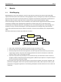
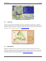
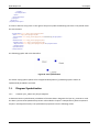
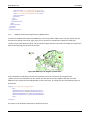
1 Basics Web Mapping is as the name indicates a term for maps that are used over the internet. Web maps offer options that extend the usual visualisation of the geographic reality of analogue maps. With the possibility to enhance maps with further interactivity elements, navigation and orientation tools and the combination of different media as sound, visuals and movies, maps are more easily interpreted (Sieber, 2009). Further advantages of web maps are the accessibility to the public and the augmented information content compared to analogue maps. Although the visualisation is still the main part of a web map, further functionalities are expected. Moreover, knowledge can be cross‐linked and generate new knowledge. The actuality of a map is a further advantage of a web map compared to an analogue map, which however comes along with expectations by the public of actuality, correctness and reliability of the map (Dickmann, 2001). A possible classification of web maps could look as follows: Web Maps Static interactive Dynamic View only View only interactive Figure 1: Map types (Kraak, 2001) •
Static maps are defined as maps that only show a map at one point in time. •
Dynamic maps are maps that show some kind of change, be it in space or time. •
View only maps have no interactive approach. For static maps this means that they consist of one single image. Dynamic maps show the changing attribute with aid of an animation or slide show. However, there is still no interaction possible. •
Interactive maps offer the possibility to interact with the map. This interaction can be in terms of navigation toolbars with panning and zooming options, different layer options or in dynamic maps in terms of animations (Cartouche, 2009). In the last few years many web maps have been set up and now circulate in the internet. However, the potential of cartographic rules has not yet been exploited (Kraak, 2001). QGIS mapserver offers a great potential for cartographic applications. The following subchapters describe the basics for the creation of a web map. 2 QGIS Mapserver 1.1.1
1 Basics Client‐server architecture Two basic architecture types can be distinguished in information technology. The first one is a local system where the user works with an operating system on which the application is directly executed. An example for this architecture is a Desktop GIS. The second architecture is the Client–Server‐architecture where the client requests data or functionality from a server. In such architecture the server is passive and waits on requests from an active client. In case of a web map the map has to be provided by a server. The client consists of any web browser that sends a request to view the map or get information about it (Cartouche, 2009). With this concept of the client‐server architecture at hand two different kinds of web maps can be kept apart: server‐sided web maps and client‐sided web maps. Client and server are connected via the internet, they only understand HTML‐messages. HTML is a markup language defined by the World Wide Web Consortium and is not extensible. So only predefined syntax can be used and understood and displayed by a web browser (W3, 2009). To display web maps a plugin has to be available which enables either the browser to display the received information or the server to translate the information into a browser‐readable format. Examples for client‐sided extensions are JavaScript or ActiveX controls. Examples for server‐sided extensions are PHP, PERL or Java servlets (Dickmann, 2001). 1.1.2
OGC The Open Geospatial Consortium consists of 382 governmental organisations, universities and companies with the aim to accelerate the development of interface specifications for geospatial data. The resulting standards are detailed interfaces and encodings that can be used to develop software which may be interoperable in the future. A document is only passed after all members have had the opportunity of commenting and discussing the standard. An unanimous resolution is aimed at for the sake of acceptance by all members. Further information can be found under www.opengeospatial.org (Reinhardt, 2004). 1.1.3
Web Map Service WMS is a specification published by the OGC to standardize the exchange of geospatial data over the internet. It consists of an http interface which enables queries for one or more geo‐coded map images from geospatial databases. The three following basic operations are standardized: •
GetCapabilities: This operation returns metadata of the requested map. •
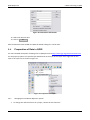
GetMap: This operation returns a map with defined referencing parameters, defined height and width of the map image, defined information and in a limited number of predefined styles. • GetFeatureInfo: This operation is optional and returns information about features in the map. The procedure of a WMS request has the following structure: 3 QGIS Mapserver 1 Basics CLIENT SERVER GetCapabilites XML document with available functionalities GetMap Display of Map GetFeatureInfo Information for certain Features Figure 2: Structure of a WMS request If the number and appearance of the predefined styles is not adequate the possibility of applying user‐
defined styles with the Styled Layer Descriptor as specified in chapter 1.1.5 Styled Layer Descriptor is available (WMS, 2006). 1.1.4
Map server A map server is basically a server that is able to answer a WMS request. The following diagram shows its purpose: Web server Server Client Map server server GIS Figure 3: Client‐Server‐Architecture A client requests functionality from a web server. A web server only comprehends HTML messages. So in case of geographical data or other complex data where the web server has to request data from a database, the web server passes the command to a map server (e.g. a Common Gateway Interface) which prepares the request for a geographical information system. A Common Gateway Interface (CGI) is a server‐sided protocol used for the linking of a web server to another program. It is an interface used for the subsequent processing of an html request that allows a called program to respond to it.1 These programs can be programmed in different programming languages. After the program handled the request, the CGI translates its results in an HTML message and forwards it to the web server. The web server receives the requested data in a readable format and displays the data in the client browser (Dickmann, 2001). As an example the following request can be interpreted: http://karlinapp.ethz.ch/fcgi‐bin/qgis_wms_dir/europe/qgis_map_serv.fcgi? SERVICE=WMS&REQUEST=GetMap&LAYERS=hillshade,cost&STYLES=default,default&BBOX=2164760,28423,
2600000,4000000&FORMAT=png&WIDTH=500&HEIGHT=500 1
A variation of the CGI is a FastCGI. The main advantage of a FCGI is the ability to process several requests with only one transport connection whereas a CGI exits an application process after responding to a request (http://www.fastcgi.com/devkit/doc/fcgi‐spec.html, 01.05.2009). 4 QGIS Mapserver 1 Basics The path points to the executable program “qgis_map_serv.fcgi” via the HTTP protocol. The successive terms after the “?” and divided by “&” define the parameters that have to be processed with the called program. 1.1.5
Styled Layer Descriptor For the display of user‐defined styles the Styled Layer Descriptor (SLD) has to be used. It is a XML standard extending the WMS Implementation Specification released by the OGC. With it symbols and colours can be rendered as wished. Therefore it allows a focus on cartographic claims. In 2007 SLD was divided into Symbology Encoding (SE) and SLD profile. Symbology Encoding is independent from service descriptions so it can also be used for user‐defined styling with other systems than services. SLD profile is the remaining part where the appliance of SE onto WMS layers is described (SE, 2006). Further extensions to the SLD‐standards have been developed, e.g. for the symbolization of diagrams (Iosifescu, 2007). 1.2.
GIS
Large amounts of data are most easily managed in databases. Data is stored in tables which hold attributes of importance. But how are geographical facts like the geometry or topology stored? In case of geographical data there are databases, called geodatabases, which have special functions to store information so that it can be visualised in geographical information systems (GIS). A GIS is defined as a system which consists of hardware, software and data. In it all data with a relation to the earth’s surface can be captured, visualised, managed, analysed and manipulated. Examples for such data are geological phenomena, the vegetation or constructions such as buildings or bridges (Reinhardt, 2009). However, a GIS is not simply a mapping program. The main advantage of using a GIS and not a simple graphics program is the possibility to give a certain object a variety of attributes. By selecting this object all attributes become visible. Furthermore the ability to analyse and manipulate data exists. The queries below can all be answered with GIS functionality: •
What river is longer than 100 km? •
How many buildings are closer to a lake than to a mountain? •
What city is built on a hill that is higher than 500 meters above sea level? Adding to this, data can be altered by applying a manipulation functionality. Examples are listed below: •
Erase all regions that are smaller than 2 km2. •
Create a buffer around all rivers. It is apparent that GIS are not only used in classical surveying or cadastral tasks. They are nowadays used in infrastructure or recycling offices, geological agencies, tourist informations and many more. Examples for such geographical information systems are ArcGIS, Geomedia or QGIS. 5 QGIS Mapserver 1.2.1
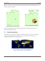
1 Basics Data formats Geospatial data can be stored in two different ways: vector data or raster data. Vector Data Vector data can be explained with various objects that fill an empty space. These objects can be points, lines or polygons and can hold any number of attributes. An example for the use of such a data structure is a dataset which contains the geometrical place of buildings (Brovelli, 2008). There are three basic types of vector data distinguishable: points, lines and polygons. Figure 4: Vector data Raster Data On the other hand, raster data are informations that cover every part of the relevant area. The area is divided into a regular grid with pixels. Each pixel can hold only one value, which is normally used for the visualisation. An example of usage is a digital terrain model or a JPEG image (Brovelli, 2008). Figure 5: Raster image 6 QGIS Mapserver 2
2 What should I know about QGIS Mapserver? What should I know about QGIS Mapserver?
•
It is an open source WMS released under the GPL2 license. Its sources are therefore freely accessible which allows all transparency possible. •
It is a FastCGI/CGI application written in C++. •
It allows the visualization and publication of maps on the internet, whether it be raster or vector data, according to cartographic rules. •
It allows the symbolization and management of geospatial data in a desktop version of QGIS. This is a user‐friendly way of symbolizing data and allows the immediate visualization of the results. With the aid of a plugin the results are easily published even without fundamental programming or scripting knowledge. •
With the extension “diagram overlay” diagrams can be generated and therefore thematic information is easily published. 2
The general public license (GPL) is a license which intends to guarantee the freedom of alternation and distribution of software (GNU, 2009). Please visit the official website at http://www.gnu.org/licenses/gpl.html for further information. 7 QGIS Mapserver 3 Installation of QGIS and QGIS Mapserver 3
Installation of QGIS and QGIS Mapserver
3.1.
Windows
All packages are available under http://karlinapp.ethz.ch/qgis_wms/download/index.html. 1. Prior to any installation of QGIS or QGIS mapserver a web server software has to be available or installed first. A good and easy to use choice for windows is wampserver which already supports the use of Apache, PHP and mySQL.3 2. Download the package “qgis_map_server.zip“ and unzip it to the directory of the cgi‐bin of your web server. Figure 6: Download of “qgis_map_server.zip” If the package is unpacked in the right directory the directory tree should look as follows: Figure 7: Folder structure in Windows 3
http://www.wampserver.com/en/ 8 QGIS Mapserver 3 Installation of QGIS and QGIS Mapserver 3. Test if QGIS mapserver is installed properly by opening a web browser and typing in the following line: http://<path to your webserver>/cgi‐bin/qgis_map_server/qgis_map_serv.cgi? SERVICE=WMS&REQUEST=GetCapabilities&Version=1.3.0 The following lines should be displayed: Figure 8: XML document with available functionalities 4. Download the package “QGISPublishToWeb.zip” and unzip it. In this package the necessary plugin “Publish to Web” is bundled with the QGIS 1.1 desktop version. 3.2.
Linux
All packages are available under http://karlinapp.ethz.ch/qgis_wms/download/index.html. 1. Prior to any installation of QGIS or QGIS mapserver a web server software has to be downloaded. The commonly used open source server Apache can be downloaded under http://httpd.apache.org/download.cgi. 2. Download the packages “qgis_mapserver_ubuntu8.04‐0.6‐bin.deb“ and “libqgis0_ubuntu8.04‐
0.11.deb“. 9 QGIS Mapserver 3 Installation of QGIS and QGIS Mapserver Figure 9: Download of “qgis_mapserver_ubuntu8.04‐0.6‐bin.deb” and ” “libqgis0_ubuntu8.04‐0.11.deb“ 3. Double click on the packages in the download list. 4. Click on 3.3.
Install Packages . Mac OS X
At the moment of the preparation of this documentation the packages for Mac OS X have not been available. Please check on http://karlinapp.ethz.ch/qgis_wms/download/index.html if they have been published. 10 QGIS Mapserver 4
4 Folder Structure of QGIS Mapserver Folder Structure of QGIS Mapserver
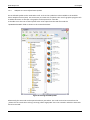
The basis for working with QGIS mapserver is to understand its file and folder structure. As explained in chapter 3 Installation of QGIS and QGIS Mapserver the main folder “qgis_map_server” is saved into the cgi‐
bin of the web server for Windows and into the fcgi‐bin of the web server for Linux. Inside this folder there are different libraries which are of no importance for simply using QGIS mapserver. Note however that there is a file called “qgis_map_serv.cgi” respectively “qgis_map_server.fcgi” for Linux which is the core element of QGIS mapserver. Another important file contained is called “admin.sld”. This is the configuration file based on SLD as described in chapter 1.1.5 Styled Layer Descriptor. Whenever a project according to chapter 5.5 Data Publishing with QGIS Mapserver is created a new folder will appear. Inside this folder a new „admin.sld“ file can be found. However, only the „admin.sld“ file inside the “qgis_map_server” folder can be published. So make sure to always copy the desired Layers into this folder. Figure 10: Basic contents of „qgis_map_server“ folder The second noticeable folder is called “qgis_wms”. It contains two folders called “Resources” and “lib”. Inside the “lib” folder there are libraries for different providers. An example is the “sosprovider.dll” which enables the linking to a sensor. These libraries may be extended. 11 QGIS Mapserver 5
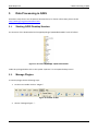
5 Data Processing in QGIS Data Processing in QGIS
Some basic steps for the use of QGIS are described here, for further information please consult http://www.qgis.org/documentation.html. 5.1.
Starting QGIS Desktop Version
The structure of the downloaded and unzipped package “QGISPublishtoWeb” looks as follows: Figure 11: Structure of package “QGISPublishtoWeb” Inside this package double click on the symbol “QGIS.exe” to start QGIS desktop version. 5.2.
Manage Plugins
To activate plugins do the following steps: 1. On the menu toolbar click on “Plugins”: Figure 12: Publish to Web 2. Choose “Manage Plugins…”. 12 QGIS Mapserver 5 Data Processing in QGIS Figure 13: Plugin Manager 3. Choose “Publish to Web”, “SPIT” or any other plugin you wish to enable. OK 4. Click on . 5. If once again clicking on „Plugins“ in the toolbar new elements in the dropdown list should be visible: Figure 14: Plugins – Publish to Web 5.3.
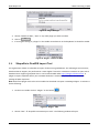
Shapefile in PostGIS Import Tool
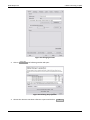
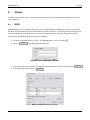
For big amounts of data it is advisable to import all data into a geodatabase. The advantages are numerous; beside multiuser support, the performance is much higher if stored in a database. PostGIS is an open source database which supports geospatial data. It can be downloaded under http://postgis.refractions.net/. A plugin to import shapefiles directly into a PostGIS database is automatically included in the download package of QGIS mapserver. Note: Before this plugin works it has to be enabled as described in chapter 5.2 Manage Plugins. To execute it do the following: 1. On the menu toolbar click on “Plugins” or the button : Figure 15: Plugins ‐ SPIT 2. Choose “SPIT” Æ “Shapefile in PostGIS Import Tool”. The following window will open: 13 QGIS Mapserver 5 Data Processing in QGIS Figure 16: Shapefile to PostGIS Import Tool 3. To set up a PostGIS connection click on New
. The following window will appear: Figure 17: New PostGIS connection 4. Enter the name, host, database name, port, user name and password of your PostGIS database. 5. Click on Test connect . 6. A pop‐up window will explain whether the connection was successful or not. If the connection failed please check your port, database and host. If it was successful click on OK . 14 QGIS Mapserver 5 Data Processing in QGIS Figure 18: Add Shapefiles to PostgreSQL 7. In the window “Shapefile in PostGIS Import Tool” click on 8. Choose the relevant shapefiles. 9. Click on OK Add
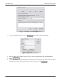
. . As a result all shapefiles have been added to the geodatabase with the chosen name on the chosen host. To import data from that database do the following: 10. Click on the button or on “Layers” Æ “Add a PostGIS Layer…”. The following window will open: Figure 19: Add PostGIS Table New 11. Click on to establish a connection to a database. “Shapefile in PostGIS Import Tool” according to chapter 5.3 Shapefile in PostGIS Import Tool will open. 15 QGIS Mapserver Figure 20: Connection Information 5 Data Processing in QGIS 12. Select the relevant data. 13. Click on Add . After all data have been loaded into QGIS the whole editing of it can be done. 5.4.
Preparation of Data in QGIS
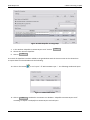
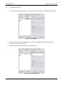
For more detailed description of editing tools in QGIS please visit http://www.qgis.org/documentation.html. For the property options of a specific layer double click on the layer in the Layers list or right click on the layer in the Layers list as shown in Figure 21. Figure 21: Properties of a layer 5.4.1
Changing the Coordinate Reference System 1. To change the reference frame of a project, choose the tab “General”. 16 QGIS Mapserver 5 Data Processing in QGIS Figure 22: Changing the CRS 2. Click on Change CRS . The following window will open: Figure 23: Defining the projection 3. Choose the relevant coordinate reference system and click on OK
. 17 QGIS Mapserver 5.4.2
5 Data Processing in QGIS Symbolization of Data 1. To symbolize data in QGIS desktop version select the tab “Symbology”. The following tab will open: Figure 24: Legend type 2. Choose the legend type. The following options are possible: Single symbol, graduated symbol, continuous color and unique value. 3. Choose the field which holds the data for the classification. Figure 25: Classification field 18 QGIS Mapserver 5 Data Processing in QGIS 4. In case of the legend type unique graduated symbol or unique value click on Figure 26: Classify Classify : 5. To change the color of any value, click on the value and the color field beside “Fill Color”. Figure 27: Changing the color 19 QGIS Mapserver 5 Data Processing in QGIS Figure 28: Choosing the color 6. With “Fill style”, “Outline color” and “Outline style” further symbolization options are possible. Figure 29: Fill style
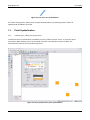
5.4.3
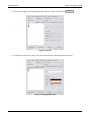
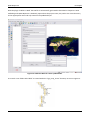
Diagram Overlay With this plugin diagrams can be generated in QGIS. Note that before this plugin works it has to be enabled as described in chapter 5.2 Manage Plugins. To execute it, do the following: 1. Double click on the layer in the Layers list which holds the data to be generated a diagram from. The following window will open: 20 QGIS Mapserver 5 Data Processing in QGIS Figure 30: Diagram Overlay 2. In the tab “diagram overlay” activate the “Display diagrams” checkbox. 3. Choose your diagram type and the classification type. 4. Add the attributes to be put into the diagram by selecting the attribute and clicking on Add attribute . 5. The colour of the attribute can be changed by double clicking on the current colour. 6. Choose the classification attribute. The diagram size will appear proportional to the value of that OK attribute. Click on to confirm. 7. In the layer property window (see Error! Reference source not found. Diagram Overlay) click on find maximum value for the program to find an appropriate size. 8. Choose your desired diagram size. 9. Click on Apply 10. Click on OK 5.5.
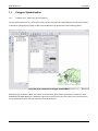
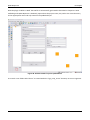
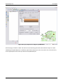
to preview your choices. . Data Publishing with QGIS Mapserver
The “Publish to Web” plugin generates a file in a XML‐schema called SLD (styled layer descriptor) which defines how the data is represented in the internet. The generated file is the configuration file and is named “admin.sld”. Before publishing your data with the mentioned plugin the data has to be prepared in QGIS. After the data looks as you wish to have it seen on the web execute this plugin. Note: Before this plugin works it has to be enabled as described in chapter 5.2 Manage Plugins. 1. In the menu toolbar in QGIS click on “Plugins” or on the button . 21 QGIS Mapserver 5 Data Processing in QGIS Figure 31: Opening the Publish to Web plugin 2. Choose “Publish to Web” Æ “Publish to Web”. The following window will open: Figure 32: Publishing the project to web 3. Enter a project name, path to the endpoint of the server directory4 and your password5. 4
The path to the endpoint of the mapserver will be as follows in Linux: “<path to your web server>/fcgi‐bin/qgis_map_server/ qgis_map_serv.fcgi?” and accordingly in Windows: “<path to your web server>/cgi‐bin/qgis_map_server/qgis_map_serv.cgi?” 4
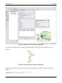
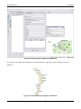
A password is only necessary when working with Linux. 22 QGIS Mapserver 5 Data Processing in QGIS 4. Fill out the service metadata. 5. Double click on the individual layers. The following window will open: Figure 33: Entering layer and style information 6. Change the name and style name to memorable names. They will be needed for further editing and have to be memorized. If desired give the Layer a Title and an abstract. 7. Click on OK . 8. Click on Publish . After this procedure the plugin saves a folder with the project name to the path specified. This should look as follows: Figure 34: Folder structure after the creation of a map Inside the newly created folder, in this example it is the folder “HazardMap", the file called “admin.sld” is saved. Opening this file shows a SLD document which defines the representation of the layers. An example of such a document can be found in 7 Examples. In chapter 5.6 Editing an „admin.sld“ file the structure of the „admin.sld“ file is explained. The published data can now be made visible with aid of a WMS client. A number of such clients is described in chapter 6 Clients. If the style of the generated „admin.sld“ file is the way it should be published, the „admin.sld“ file has to be copied into the “q_gis_map_server” folder because only if the „admin.sld“ file is in this position of the folder structure it is published. 23 QGIS Mapserver 5.6.
Editing an „admin.sld“ file
5.6.1
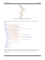
Structure 5 Data Processing in QGIS As earlier mentioned the „admin.sld“ file is the heart of QGIS mapserver. All configurations are made with this file. Understanding how to edit this file leads to a variety of visualisation possibilities. For simple symbologies, such as plain fills of polygons or strokes, the file does not have to be edited manually. However, if more complex structures or individual patterns are intended to be visualised the „admin.sld“ file has to be edited manually. Examples of the editing are demonstrated in chapter 7 Examples. The basic structure of an „admin.sld“ file is as follows: <StyledLayerDescriptor> Root element: start of sld‐file <UserLayer> Start of layer <Name></Name> Name of layer <Title></Title> Title of layer <Abstract></Abstract> Description of layer <HostedVDS/> Data Source of layer <UserStyle> Start of style <Name></Name> Name of style </UserStyle> End of style </UserLayer> End of layer </StyledLayerDescriptor> End of .sld‐file
Figure 35: Basic structure of an „admin.sld“ file This structure is generated automatically when a project is created with the „Publish to Web“ plugin provided by QGIS mapserver. The succeeding example shows an „admin.sld“ file which defines a raster layer. For feature layers there are further definitions to be found: Inside the <UserStyle> tag there is a number of subtabs. This may look as follows: 24 QGIS Mapserver 5 Data Processing in QGIS <UserStyle xmlns="http://www.opengis.net/sld"> Start of style <Name xmlns="http://www.opengis.net/sld">Single Symbol</Name> Name of style <FeatureTypeStyle xmlns="http://www.opengis.net/sld"> Style for feature layer <Rule xmlns="http://www.opengis.net/sld"> Start of rule <PointSymbolizer xmlns="http://www.opengis.net/sld"> Symbolizing option <Graphic xmlns="http://www.opengis.net/sld"> <Mark xmlns="http://www.opengis.net/sld"> <WellKnownName xmlns="http://www.opengis.net/sld">rectangle</WellKnownName> <Stroke xmlns="http://www.opengis.net/sld"> Definition of stroke <CssParameter xmlns="http://www.opengis.net/sld" Definition of stroke color :name="stroke">#000000</CssParameter> <CssParameter xmlns="http://www.opengis.net/sld" :name="stroke‐width" Definition of stroke‐width >0</CssParameter> </Stroke> <Fill xmlns="http://www.opengis.net/sld"> Definition of fill <CssParameter xmlns="http://www.opengis.net/sld" :name="fill" Definition of fill color >#afa3a4</CssParameter> </Fill> End of fill </Mark> End of mark <Size xmlns="http://www.opengis.net/sld">2.2</Size> Definition of size </Graphic> End of graphic </PointSymbolizer> End of symbolizing option </Rule> End of rule </FeatureTypeStyle> End of feature layer style </UserStyle> End of style Figure 36: Structure of the tag UserStyle 5.6.2
Symbolizers Depending on whether the object to be displayed is a point, line, polygon, text or diagram different symbolizing options can be used: <PointSymbolizer> Point symbol
<LineSymbolizer> Line symbol <PolygonSymbolizer> Polygon symbol <TextSymbolizer> Text Symbol <DiagramSymbolizer> Diagram symbol Figure 37: Symbolizers Within these symbolization options numerous definitions can be changed. A list of implemented options can be found in Appendix B Definition of symbolizing options. Note that not all standards as published by the OGC in Document # 05‐078r4 are yet supported. 25 QGIS Mapserver 5.6.3
5 Data Processing in QGIS Filter Encoding Another implementation is called filter encoding. With this the Filter Encoding Implementation Specifications published by the OGC are supported. Therefore symbolization depending on an attribute value is possible. For an example please consult chapter 7.1.4 Filter Encoding. 26 QGIS Mapserver 6
6 Clients Clients
To display the prepared map in a web browser a framework client is needed. All described clients are open source products. 6.1.
QGIS
QGIS desktop version is a WMS Client as well. The main advantage of using QGIS as a client is the easy and fast display of data without having to deal with source codes. However, it is a client‐sided extension that has to be downloaded and unpacked first. If a map is to be published on the web, this client cannot be used. To view maps with QGIS desktop version do the following: 1. On the menu toolbar click on “Layers” Æ “Add WMS Layer” or on the symbol 2. Click on New . The following window will open: Figure 38: Create a new WMS connection 3. Insert a name for the connection and the URL to the WMS layer you wish to add. Click on 4. In the following window click on Connect
OK
. . Figure 39: Add Layer(s) from a server 27 QGIS Mapserver 6 Clients 5. Choose the desired layer by clicking on the + beside the layer, then choosing the User Style (in this example “per”). Choosing the User Style leads to the visualisation of the layer as described in the „admin.sld“ file. If the layer itself is added (in this example “Perimeter”) then the symbolization is not added. This means the layer will appear with default styling which is in black strokes without any fills. 6. Change the coordinate system if required by clicking on 7. Clicking on Add Change ...
completes the procedure. Figure 40: Example of a QGIS map 6.2.
. Open Layers
Open Layers is a free Javascript library which allows dynamic maps to be displayed in any web browser without any server‐sided dependencies. It offers diverse widgets for easily implementing functions as zooming, panning or centering to any displayed map. OpenLayers offers an extensive gallery with examples for its utilization. For further information please visit http://openlayers.org/. An example of the integration of a map in Open Layers can be found in Appendix A Example of the integration of an „admin.sld“ file in OpenLayers. 28 QGIS Mapserver Figure 41: Example of an Open Layers map 6.3.
6 Clients Carto.net
Carto.net is a framework client developed by the institute of cartography at the ETH Zurich. It is based on JavaScript and SVG and offers a list of widgets. For reasons of popularity of JavaScript the visualisation of the framework client has many options. The only disadvantage of this client is the rather short documentation of the product. Further information can be found on http://www.carto.net. Figure 42: Example of a Cartonet map (CARTONET, 2009) 6.4.
Map Bender
MapBender is programmed in PHP and JavaScript and supports PostGIS and MySQL databases. A great advantage of this client is the comprehensive documentation in a Wiki. It also offers many tools as zooming or panning . A further useful tool is the offering of authentication and authorization services. The following link provides detailed information about the product: http://www.mapbender.org. 29 QGIS Mapserver Figure 43: Example of a MapBender map (MapBender, 2009) 6 Clients 30 QGIS Mapserver 7
7 Examples Examples
The following pages offer different examples of the creation of a web map for different data types. The used dataset is a generalized dataset which comprises of feature data (countries) that are derived from the CIA World DataBank II and a satellite image by NASA. Futhermore, a simple point and line layer are used. All data, intermediate results and definitive results can be found in the ZIP folder complementing this User Manual. If the data is used, make sure to change the path in the “HostedVDS” tag to the directory that contains the data. The general workflow for the production of a web map is the following: 1.
2.
3.
4.
5.
6.
7.
Installation of a webserver Installation of QGIS mapserver Download of QGIS desktop version Data Processing in QGIS desktop version Publishing Data Editing the „admin.sld“ file Integration of the map in a framework client Chapter 3 Installation of QGIS and QGIS Mapserver Chapter 3 Installation of QGIS and QGIS Mapserver Chapter 3 Installation of QGIS and QGIS Mapserver Chapter 5 Data Processing in QGIS Chapter 5.5 Data Publishing with QGIS Mapserver Chapter 5.6 Editing an „admin.sld“ file Chapter 6 Clients All examples presume a completion of steps 1 to 3, which is the proper installation of a webserver and QGIS mapserver (see chapter 3 Installation of QGIS and QGIS Mapserver), opening QGIS desktop version (chapter 5.1 Starting QGIS Desktop Version), management of plugins (chapter 5.2 Manage Plugins) and the management of data (chapter 5.3 Shapefile in PostGIS Import Tool). 31 QGIS Mapserver 7.1.
Polygon Symbolization
7.1.1
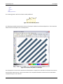
Creation of an „admin.sld“ file for Polygons 7 Examples For this example the layer eu_countries is used. The data is processed in QGIS desktop version as described in chapter 5.4 Preparation of Data in QGIS. The symbolization properties have the following values: Figure 44: Layer properties for polygon symbolization With the plugin “Publish to Web” the SLD‐file is automatically generated as described in chapter 5.5 Data Publishing with QGIS Mapserver. Absolutely required are the project name, the path to the server directory and an appropriate name and style name for the published layer. 32 QGIS Mapserver 7 Examples Figure 45: Publish to Web for polygon symbolization As a result a new folder called “Countries” is created inside the “qgis_map_server” directory as seen in Figure 46. Figure 46: Folder structure for polygon symbolization Inside this folder the file called “admin.sld” can be opened with any text editor. It will be structured as follows: <StyledLayerDescriptor xmlns="http://www.opengis.net/sld" units="mm" > <UserLayer xmlns="http://www.opengis.net/sld"> 33 QGIS Mapserver 7 Examples <Name xmlns="http://www.opengis.net/sld">Countries</Name> <Title xmlns="http://www.opengis.net/sld"></Title> <Abstract xmlns="http://www.opengis.net/sld"></Abstract> <HostedVDS xmlns="http://www.opengis.net/sld" providerType="ogr" uri="U:\user\geodata_eu\eu_countries_them.shp" /> <UserStyle xmlns="http://www.opengis.net/sld"> <Name xmlns="http://www.opengis.net/sld">country</Name> <FeatureTypeStyle xmlns="http://www.opengis.net/sld"> <Rule xmlns="http://www.opengis.net/sld"> <Filter xmlns="http://www.opengis.net/ogc"> <PropertyIsBetween xmlns="http://www.opengis.net/ogc"> <PropertyName xmlns="http://www.opengis.net/ogc">SERVICE</PropertyName> <LowerBoundary xmlns="http://www.opengis.net/ogc"> <Literal xmlns="http://www.opengis.net/ogc">‐0.001</Literal> </LowerBoundary> <UpperBoundary xmlns="http://www.opengis.net/ogc"> <Literal xmlns="http://www.opengis.net/ogc">6975.500</Literal> </UpperBoundary> </PropertyIsBetween> </Filter> <PolygonSymbolizer xmlns="http://www.opengis.net/sld"> <Stroke xmlns="http://www.opengis.net/sld"> <CssParameter xmlns="http://www.opengis.net/sld" :name="stroke" >#000000</CssParameter> <CssParameter xmlns="http://www.opengis.net/sld" :name="stroke‐width" >1</CssParameter> </Stroke> <Fill xmlns="http://www.opengis.net/sld"> <CssParameter xmlns="http://www.opengis.net/sld" :name="fill" >#daffc9</CssParameter> </Fill> </PolygonSymbolizer> </Rule> <Rule xmlns="http://www.opengis.net/sld"> <Filter xmlns="http://www.opengis.net/ogc"> <PropertyIsBetween xmlns="http://www.opengis.net/ogc"> <PropertyName xmlns="http://www.opengis.net/ogc">SERVICE</PropertyName> <LowerBoundary xmlns="http://www.opengis.net/ogc"> <Literal xmlns="http://www.opengis.net/ogc">6975.500</Literal> </LowerBoundary> <UpperBoundary xmlns="http://www.opengis.net/ogc"> <Literal xmlns="http://www.opengis.net/ogc">13951.000</Literal> </UpperBoundary> </PropertyIsBetween> </Filter> <PolygonSymbolizer xmlns="http://www.opengis.net/sld"> <Stroke xmlns="http://www.opengis.net/sld"> <CssParameter xmlns="http://www.opengis.net/sld" :name="stroke" >#000000</CssParameter> <CssParameter xmlns="http://www.opengis.net/sld" :name="stroke‐width" >1</CssParameter> </Stroke> <Fill xmlns="http://www.opengis.net/sld"> <CssParameter xmlns="http://www.opengis.net/sld" :name="fill" >#a1bb94</CssParameter> </Fill> </PolygonSymbolizer> </Rule> <Rule xmlns="http://www.opengis.net/sld"> <Filter xmlns="http://www.opengis.net/ogc"> <PropertyIsBetween xmlns="http://www.opengis.net/ogc"> <PropertyName xmlns="http://www.opengis.net/ogc">SERVICE</PropertyName> <LowerBoundary xmlns="http://www.opengis.net/ogc"> <Literal xmlns="http://www.opengis.net/ogc">13951.000</Literal> </LowerBoundary> <UpperBoundary xmlns="http://www.opengis.net/ogc"> <Literal xmlns="http://www.opengis.net/ogc">20926.500</Literal> </UpperBoundary> 34 QGIS Mapserver 7 Examples </PropertyIsBetween> </Filter> <PolygonSymbolizer xmlns="http://www.opengis.net/sld"> <Stroke xmlns="http://www.opengis.net/sld"> <CssParameter xmlns="http://www.opengis.net/sld" :name="stroke" >#000000</CssParameter> <CssParameter xmlns="http://www.opengis.net/sld" :name="stroke‐width" >1</CssParameter> </Stroke> <Fill xmlns="http://www.opengis.net/sld"> <CssParameter xmlns="http://www.opengis.net/sld" :name="fill" >#869b7b</CssParameter> </Fill> </PolygonSymbolizer> </Rule> <Rule xmlns="http://www.opengis.net/sld"> <Filter xmlns="http://www.opengis.net/ogc"> <PropertyIsBetween xmlns="http://www.opengis.net/ogc"> <PropertyName xmlns="http://www.opengis.net/ogc">SERVICE</PropertyName> <LowerBoundary xmlns="http://www.opengis.net/ogc"> <Literal xmlns="http://www.opengis.net/ogc">20926.500</Literal> </LowerBoundary> <UpperBoundary xmlns="http://www.opengis.net/ogc"> <Literal xmlns="http://www.opengis.net/ogc">27902.001</Literal> </UpperBoundary> </PropertyIsBetween> </Filter> <PolygonSymbolizer xmlns="http://www.opengis.net/sld"> <Stroke xmlns="http://www.opengis.net/sld"> <CssParameter xmlns="http://www.opengis.net/sld" :name="stroke" >#000000</CssParameter> <CssParameter xmlns="http://www.opengis.net/sld" :name="stroke‐width" >1</CssParameter> </Stroke> <Fill xmlns="http://www.opengis.net/sld"> <CssParameter xmlns="http://www.opengis.net/sld" :name="fill" >#62735b</CssParameter> </Fill> </PolygonSymbolizer> </Rule> </FeatureTypeStyle> </UserStyle> </UserLayer> </StyledLayerDescriptor> To view the symbolization of this file a WMS layer can be imported in QGIS. To do that the „admin.sld“ file first has to be placed in the main „qgis_map_server“ directory as explained in chapter 5.6 Editing an „admin.sld“ file. Afterwards this layer can be opened in QGIS with the instructions of chapter 6.1 QGIS which leads to the following visualization of the style: Figure 47: WMS layer for polygon symbolization 35 QGIS Mapserver 7.1.2
7 Examples Adaption of the Dasharray of an Outline Stroke If this visualization result does not turn out satisfactory the style can directly be changed in the „admin.sld“ file. The outline color which is at the moment black and a solid line wants to be changed to a darkbrown color and dashed line. To do this all stroke paragraphs have to be changed into the following code: <Stroke xmlns="http://www.opengis.net/sld"> <CssParameter xmlns="http://www.opengis.net/sld" :name="stroke" >#000000</CssParameter> <CssParameter xmlns="http://www.opengis.net/sld" :name="stroke‐width" >1</CssParameter> <CssParameter xmlns="http://www.opengis.net/sld" :name="stroke‐dasharray">2 1 3</CssParameter> </Stroke> The result can be viewed in QGIS after a reload of the layer. Note: To refresh the layer visualization move the layer with the panning tool in QGIS desktop version. The outline strokes will change consequently: Figure 48: Outline style polygon symbolization 7.1.3
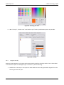
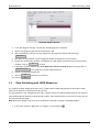
Creation of a User‐defined Pattern in SVG A very useful functionality is the implementation of user‐defined patterns. To do so the pattern has to be available in the Scalable Vector Graphics format (SVG). The easiest way to create such a pattern is the use of a graphics program such as Adobe Illustrator or Inkscape. The graphic can be exported as a SVG‐File and opened in any text editor. Inside the polygon symbolizer and the fill‐tag a new tag named <pattern> has to be created with the size of the SVG‐pattern. Inside the tag <pattern> a new group <g> is implemented in which the SVG‐symbol is pasted from the text document. The example below shows the structure the “admin.sld” file should have after the editing: <PolygonSymbolizer xmlns="http://www.opengis.net/sld"> <Stroke xmlns="http://www.opengis.net/sld"> <CssParameter xmlns="http://www.opengis.net/sld" :name="stroke" >#000000</CssParameter> <CssParameter xmlns="http://www.opengis.net/sld" :name="stroke‐width" >0</CssParameter> </Stroke> <Fill xmlns="http://www.opengis.net/sld"> <pattern x="0" y="0" width="12" height="12"> <g> <svg> <g> <rect style="fill:none;" width="12" height="12"/> <line style="fill:none;stroke:#FEDC00;stroke‐width:2;" x1="6" y1="12" x2="6" y2="0"/> </g> 36 QGIS Mapserver 7 Examples </svg> </g> </pattern> </Fill> </PolygonSymbolizer> The resulting pattern will look as follows when published: Figure 49: User‐defined pattern The following example demonstrates the use of Inkscape to define more advanced patterns. The screenshot below shows an example of the created pattern: Figure 50: Creation of a pattern in Inkscape This Inkscape‐file is saved in the SVG format. Afterwards it is opened in a text editor and shows the structure shown below. Note that this is only an extraction of the complete file which can be found in the ZIP folder complementing this User Manual. 37 QGIS Mapserver 7 Examples <?xml version="1.0" encoding="iso‐8859‐1"?> <!‐‐ Generator: Adobe Illustrator 13.0.2, SVG Export Plug‐In . SVG Version: 6.00 Build 14948) ‐‐> <!DOCTYPE svg PUBLIC "‐//W3C//DTD SVG 1.1//EN" "http://www.w3.org/Graphics/SVG/1.1/DTD/svg11.dtd"> <svg … </svg> This code is now included in the „admin.sld“ file until it looks as seen in the following code: <PolygonSymbolizer xmlns="http://www.opengis.net/sld"> <Fill xmlns="http://www.opengis.net/sld"> <pattern width="29" height="29" x="0" y="0"> <g> <svg xmlns:dc="http://purl.org/dc/elements/1.1/" xmlns:cc="http://creativecommons.org/ns#" xmlns:rdf="http://www.w3.org/1999/02/22‐rdf‐syntax‐ns#" xmlns:svg="http://www.w3.org/2000/svg" xmlns=http://www.w3.org/2000/svg … </svg> </g> </pattern> </Fill> </PolygonSymbolizer> The code leads to the following result: Figure 51: User‐defined pattern created in Inkscape 7.1.4
Filter Encoding Another helpful symbolization option is the use of filter encoding. With it objects with a certain attribute value can be symbolized separately. The following code shows an example of its use. All objects that have a value between ‐0.001 and 6975.500 in the attribute called “SERVICE” will be symbolized as defined between the <PolygonSymbolizer>‐tags. <Rule xmlns="http://www.opengis.net/sld"> <Filter xmlns="http://www.opengis.net/ogc"> <PropertyIsBetween xmlns="http://www.opengis.net/ogc"> <PropertyName xmlns="http://www.opengis.net/ogc">SERVICE</PropertyName> <LowerBoundary xmlns="http://www.opengis.net/ogc"> <Literal xmlns="http://www.opengis.net/ogc">‐0.001</Literal> </LowerBoundary> <UpperBoundary xmlns="http://www.opengis.net/ogc"> <Literal xmlns="http://www.opengis.net/ogc">6975.500</Literal> 38 QGIS Mapserver 7 Examples </UpperBoundary> </PropertyIsBetween> </Filter> <PolygonSymbolizer xmlns="http://www.opengis.net/sld"> <Stroke xmlns="http://www.opengis.net/sld"> <CssParameter xmlns="http://www.opengis.net/sld" :name="stroke" >#000000</CssParameter> <CssParameter xmlns="http://www.opengis.net/sld" :name="stroke‐width" >0</CssParameter> </Stroke> <Fill xmlns="http://www.opengis.net/sld"> <CssParameter xmlns="http://www.opengis.net/sld" :name="fill" >#daffc9</CssParameter> </Fill> </PolygonSymbolizer> </Rule> For further styling options please refer to Appendix B Definition of symbolizing options where all implemented possibilities are listed. 39 QGIS Mapserver 7.2.
Line Symbolization
7.2.1
Creation of an „admin.sld“ file for Lines 7 Examples For this symbolization method the layer “Line” is used. The data is processed in QGIS desktop version as described in chapter 5.4 Preparation of Data in QGIS. The symbolization properties have the following values: Figure 52: Layer properties for line symbolization With the plugin “Publish to Web” the SLD‐file is automatically generated as described in chapter 5.5 Data Publishing with QGIS Mapserver. Absolutely required are the project name, the path to the server directory and an appropriate name and style name for the published layer. 40 QGIS Mapserver 7 Examples Figure 53: Publish to Web for line symbolization As a result a new folder called “Line” is created inside the “qgis_map_server” directory as seen in Figure 54. Figure 54: Folder structure for line symbolization Inside this folder the file called “admin.sld” can be opened with any text editor. It will be structured as follows: 41 QGIS Mapserver 7 Examples <StyledLayerDescriptor xmlns="http://www.opengis.net/sld" units="mm" > <UserLayer xmlns="http://www.opengis.net/sld"> <Name xmlns="http://www.opengis.net/sld">Line</Name> <Title xmlns="http://www.opengis.net/sld"></Title> <Abstract xmlns="http://www.opengis.net/sld"></Abstract> <HostedVDS xmlns="http://www.opengis.net/sld" providerType="ogr" uri="D:/LineExamples/Line" /> <UserStyle xmlns="http://www.opengis.net/sld"> <Name xmlns="http://www.opengis.net/sld">line</Name> <FeatureTypeStyle xmlns="http://www.opengis.net/sld"> <Rule xmlns="http://www.opengis.net/sld"> <LineSymbolizer xmlns="http://www.opengis.net/sld"> <Stroke xmlns="http://www.opengis.net/sld"> <CssParameter xmlns="http://www.opengis.net/sld" :name="stroke" >#79aee5</CssParameter> <CssParameter xmlns="http://www.opengis.net/sld" :name="stroke‐width" >10</CssParameter> </Stroke> </LineSymbolizer> </Rule> </FeatureTypeStyle> </UserStyle> </UserLayer> </StyledLayerDescriptor> To view the symbolization of this file a WMS layer can be imported in QGIS. To do that the „admin.sld“ file first has to be placed in the main “qgis_map_server” directory as explained in chapter 5.6 Editing an „admin.sld“ file. Afterwards this layer can be opened in QGIS with the instructions of chapter 6.1 QGIS which leads to the following visualization of the style: Figure 55: Extract of a WMS layer for line symbolization 7.2.2
Adaption of the Line cap If this visualization result does not turn out satisfactory the style can directly be changed in the „admin.sld“ file. The symbolization of the river is in a light blue color with square line caps. For rounded line caps the stroke code has to be changed into the following lines: <Stroke xmlns="http://www.opengis.net/sld"> <CssParameter xmlns="http://www.opengis.net/sld" :name="stroke" >#79aee5</CssParameter> <CssParameter xmlns="http://www.opengis.net/sld" :name="stroke‐width" >10</CssParameter> <CssParameter xmlns="http://www.opengis.net/sld" :name="stroke‐linecap" >round</CssParameter> </Stroke> The result can be viewed in QGIS after a reload of the layer. Note: To refresh the layer visualization move the layer with the panning tool in QGIS desktop version. The line cap will change consequently: 42 QGIS Mapserver 7 Examples Figure 56: Line cap in line symbolization For further styling options please refer to Appendix B Definition of symbolizing options where all implemented possibilities are listed. 7.3.
Point Symbolization
7.3.1
Creation of an „admin.sld“ file for Points To demonstrate the symbolization possibilities of point symbols the layer “Point” is used. The data is processed in QGIS desktop version as described in chapter 5.4 Preparation of Data in QGIS. The symbolization properties have the following values: Figure 57: Layer properties for point symbolization 43 QGIS Mapserver 7 Examples With the plugin “Publish to Web” the SLD‐file is automatically generated as described in chapter 5.5 Data Publishing with QGIS Mapserver. Absolutely required are the project name, the path to the server directory and an appropriate name and style name for the published layer. Figure 58: Publish to Web for point symbolization As a result a new folder called “Point” is created inside the “qgis_map_server” directory as seen in Figure 59. 44 QGIS Mapserver 7 Examples Figure 59: Folder structure for point symbolization Inside this folder the file called “admin.sld” can be opened with any text editor. It will be structured as follows: <StyledLayerDescriptor xmlns="http://www.opengis.net/sld" units="mm" > <UserLayer xmlns="http://www.opengis.net/sld"> <Name xmlns="http://www.opengis.net/sld">Point</Name> <Title xmlns="http://www.opengis.net/sld"></Title> <Abstract xmlns="http://www.opengis.net/sld"></Abstract> <HostedVDS xmlns="http://www.opengis.net/sld" providerType="ogr" uri="D:\PointExample\Point.shp" /> <UserStyle xmlns="http://www.opengis.net/sld"> <Name xmlns="http://www.opengis.net/sld">point</Name> <FeatureTypeStyle xmlns="http://www.opengis.net/sld"> <Rule xmlns="http://www.opengis.net/sld"> <PointSymbolizer xmlns="http://www.opengis.net/sld"> <Graphic xmlns="http://www.opengis.net/sld"> <Mark xmlns="http://www.opengis.net/sld"> <WellKnownName xmlns="http://www.opengis.net/sld">rectangle</WellKnownName> <Stroke xmlns="http://www.opengis.net/sld"> <CssParameter xmlns="http://www.opengis.net/sld" :name="stroke" >#000000</CssParameter> <CssParameter xmlns="http://www.opengis.net/sld" :name="stroke‐width" >0</CssParameter> </Stroke> <Fill xmlns="http://www.opengis.net/sld"> <CssParameter xmlns="http://www.opengis.net/sld" :name="fill" >#ffa914</CssParameter> </Fill> </Mark> <Size xmlns="http://www.opengis.net/sld">15</Size> </Graphic> </PointSymbolizer> </Rule> </FeatureTypeStyle> </UserStyle> </UserLayer> </StyledLayerDescriptor> To view the symbolization of this file a WMS layer can be imported in QGIS. To do that the „admin.sld“ file first has to be placed in the main „qgis_map_server“ directory as explained in chapter 5.6 Editing an „admin.sld“ file. 45 QGIS Mapserver 7 Examples Note: This procedure is at the moment only automatically possible with some well‐known‐name object such as circle or square. Other symbols have to be manually changed by editing the „admin.sld“ file which will be explained on the next page. 7.3.2
Adaption to a different Point Symbol After the described procedure this layer can be opened in QGIS with the instructions of chapter 6.1 QGIS which leads to the following visualization of the style: Figure 60: Extract of a WMS layer for point symbolization If this visualization result does not turn out satisfactory the style can directly be changed in the „admin.sld“ file. At the moment the point symbols are orange squares. To change that symbolization to another well‐known‐name symbol exchange the WellKnownName‐tag with the following: <WellKnownName xmlns="http://www.opengis.net/sld">star</WellKnownName> The result can be viewed in QGIS after a reload of the layer. Note: To refresh the layer visualization move the layer with the panning tool in QGIS desktop version. The symbol will change consequently: Figure 61: Line cap in line symbolization 46 QGIS Mapserver 7.3.3
7 Examples Adaption to a User‐defined Point Symbol A user‐defined symbol can be visualized as well. To do so the symbol has to be available in the Scalable Vector Graphics‐format (SVG). The easiest way to create such a symbol is the use of a graphics program such as Adobe Illustrator or Inkscape. The graphic can be exported as a SVG file. To be able to use this user created symbol it has to be copied into the SVG‐file inside the “QGISPublishtoWeb” folder as shown in the screenshot below: Figure 62: Placing the SVG‐Symbol Alternatively the SVG code can be opened inside any text editor. The code can then be inserted into the „admin.sld“ file. Inside the mark‐tag a new tag called “SvgSymbol” has to be created in which the SVG‐code has to be inserted: 47 QGIS Mapserver 7 Examples <Mark xmlns="http://www.opengis.net/sld"> <SvgSymbol xmlns="http://www.opengis.net/sld"> <svg width="100%" height="100%" xmlns="http://www.w3.org/2000/svg"> <g xmln="http://www.w2.org/2000/svg"> <rect x="0" y="0" height="30" width="30" style="fill:#0000b9"/> <line x1="6" y1="0" x2="30" y2="12" style="stroke:#00ffff"/> </g> </svg> </SvgSymbol> </Mark> The following output is created: Figure 63: User‐defined symbolization For further styling options please refer to Appendix B Definition of symbolizing options where all implemented possibilities are listed. 7.4.
Text Symbolization
Text symbolization is not yet implemented to appear automatically. However by editing an „admin.sld“ file manually labels can easily be displayed. The following SLD‐file shows the point symbolization from the example above. <StyledLayerDescriptor xmlns="http://www.opengis.net/sld" units="mm" > <UserLayer xmlns="http://www.opengis.net/sld"> <Name xmlns="http://www.opengis.net/sld">Point</Name> <Title xmlns="http://www.opengis.net/sld"></Title> <Abstract xmlns="http://www.opengis.net/sld"></Abstract> <HostedVDS xmlns="http://www.opengis.net/sld" providerType="ogr" uri="D:\PointExample\Point.shp" /> <UserStyle xmlns="http://www.opengis.net/sld"> <Name xmlns="http://www.opengis.net/sld">point</Name> <FeatureTypeStyle xmlns="http://www.opengis.net/sld"> <Rule xmlns="http://www.opengis.net/sld"> <PointSymbolizer xmlns="http://www.opengis.net/sld"> <Graphic xmlns="http://www.opengis.net/sld"> <Mark xmlns="http://www.opengis.net/sld"> <SvgSymbol xmlns="http://www.opengis.net/sld"> <svg width="100%" height="100%" xmlns="http://www.w3.org/2000/svg"> <g xmln="http://www.w2.org/2000/svg"> <rect x="0" y="0" height="30" width="30" style="fill:#0000b9"/> <line x1="6" y1="0" x2="30" y2="12" style="stroke:#00ffff"/> </g> </svg> </SvgSymbol> </Mark> <Size xmlns="http://www.opengis.net/sld">15</Size> 48 QGIS Mapserver 7 Examples </Graphic> </PointSymbolizer> </Rule> </FeatureTypeStyle> </UserStyle> </UserLayer> </StyledLayerDescriptor> To insert a label for every point on the right of the point symbol the following lines have to be placed inside the rule‐element: <TextSymbolizer xmlns="http://www.opengis.net/sld"> <Label xmlns="http://www.opengis.net/sld"> <PropertyName xmlns="http://www.opengis.net/sld">PointExamp</PropertyName> </Label> <LabelPlacement xmlns="http://www.opengis.net/sld"> <PointPlacement xmlns="http://www.opengis.net/sld"> <DisplacementX xmlns="http://www.opengis.net/sld">30</DisplacementX> </PointPlacement> </LabelPlacement> </TextSymbolizer> The following graphic will result thereafter: Figure 64: Text symbolization For further styling options please refer to Appendix B Definition of symbolizing options where all implemented possibilities are listed. 7.5.
Diagram Symbolization
7.5.1
Creation of an „admin.sld“ file for Diagrams To demonstrate the symbolization possibilities of thematic data in diagrams the layer eu_countries is used. The data is processed in QGIS desktop version as described in chapter 5.4 Preparation of Data in QGIS and chapter 5.4.3 Diagram Overlay. The symbolization properties have the following values: 49 QGIS Mapserver 7 Examples Figure 65: Layer properties for diagram symbolization With the plugin “Publish to Web” the SLD file is automatically generated as described in chapter 5.5 Data Publishing with QGIS Mapserver. Absolutely required are the project name, the path to the server directory and an appropriate name and style name for the published layer. 50 QGIS Mapserver 7 Examples Figure 66: Publish to Web for diagram symbolization As a result a new folder called “Diagrams” is created inside the “qgis_map_server” directory as seen in Figure 67. Figure 67: Folder structure for diagram symbolization 51 QGIS Mapserver 7 Examples Inside this folder the file called “admin.sld” can be opened with any text editor. It will be structured as follows: <StyledLayerDescriptor xmlns="http://www.opengis.net/sld" units="mm" > <UserLayer xmlns="http://www.opengis.net/sld"> <Name xmlns="http://www.opengis.net/sld">Diagrams</Name> <Title xmlns="http://www.opengis.net/sld"></Title> <Abstract xmlns="http://www.opengis.net/sld"></Abstract> <HostedVDS xmlns="http://www.opengis.net/sld" providerType="ogr" uri="D:\user\geodata_eu\eu_countries_them.shp" /> <UserStyle xmlns="http://www.opengis.net/sld"> <Name xmlns="http://www.opengis.net/sld">diagram</Name> <FeatureTypeStyle xmlns="http://www.opengis.net/sld"> <Rule xmlns="http://www.opengis.net/sld"> <PolygonSymbolizer xmlns="http://www.opengis.net/sld"> <Stroke xmlns="http://www.opengis.net/sld"> <CssParameter xmlns="http://www.opengis.net/sld" :name="stroke" >#000000</CssParameter> <CssParameter xmlns="http://www.opengis.net/sld" :name="stroke‐width" >0</CssParameter> </Stroke> <Fill xmlns="http://www.opengis.net/sld"> <CssParameter xmlns="http://www.opengis.net/sld" :name="fill" >#daffc9</CssParameter> </Fill> </PolygonSymbolizer> </Rule> <Rule xmlns="http://www.opengis.net/sld"> <DiagramSymbolizer xmlns="http://www.opengis.net/sld"> <Diagram xmlns="http://www.opengis.net/sld"> <WellKnownName xmlns="http://www.opengis.net/sld">Pie</WellKnownName> <Category xmlns="http://www.opengis.net/sld"> <PropertyName xmlns="http://www.opengis.net/ogc">INDUSTRY</PropertyName> <SvgParameter :name="fill" >#ffba7e</SvgParameter> </Category> <Category xmlns="http://www.opengis.net/sld"> <PropertyName xmlns="http://www.opengis.net/ogc">SERVICE</PropertyName> <SvgParameter :name="fill" >#d19767</SvgParameter> </Category> <Category xmlns="http://www.opengis.net/sld"> <PropertyName xmlns="http://www.opengis.net/ogc">CONSTRUCTI</PropertyName> <SvgParameter :name="fill" >#c08b5f</SvgParameter> </Category> <Category xmlns="http://www.opengis.net/sld"> <PropertyName xmlns="http://www.opengis.net/ogc">AGRICULTUR</PropertyName> <SvgParameter :name="fill" >#a67852</SvgParameter> </Category> <Category xmlns="http://www.opengis.net/sld"> <PropertyName xmlns="http://www.opengis.net/ogc">FINANCIAL</PropertyName> <SvgParameter :name="fill" >#815d3f</SvgParameter> </Category> <Category xmlns="http://www.opengis.net/sld"> <PropertyName xmlns="http://www.opengis.net/ogc">WHOLESALE</PropertyName> <SvgParameter :name="fill" >#4a3524</SvgParameter> </Category> <Size xmlns="http://www.opengis.net/sld"> <Interpolate xmlns="http://www.opengis.net/ogc" mode="linear" > <LookupValue xmlns="http://www.opengis.net/sld"> <PropertyName xmlns="http://www.opengis.net/ogc">TOTALEMPL</PropertyName> </LookupValue> <InterpolationPoint xmlns="http://www.opengis.net/sld"> <Data xmlns="http://www.opengis.net/sld">0</Data> <Value xmlns="http://www.opengis.net/sld">0</Value> </InterpolationPoint> 52 QGIS Mapserver 7 Examples <InterpolationPoint xmlns="http://www.opengis.net/sld"> <Data xmlns="http://www.opengis.net/sld">68169</Data> <Value xmlns="http://www.opengis.net/sld">10</Value> </InterpolationPoint> </Interpolate> </Size> </Diagram> </DiagramSymbolizer> </Rule> </FeatureTypeStyle> </UserStyle> </UserLayer> </StyledLayerDescriptor> 7.5.2
Adaption of the Zoom Dependency of Diagram Size To view the symbolization of this file a WMS layer can be imported in QGIS. To do that the „admin.sld“ file first has to be placed in the main „qgis_map_server“ directory as explained in chapter 5.6 Editing an „admin.sld“ file. Afterwards this layer can be opened in QGIS with the instructions of chapter 6.1 QGIS which leads to the following visualization of the style: Figure 68: WMS layer for diagram symbolization If this visualization result does not turn out satisfactory the style can directly be changed in the „admin.sld“ file. The visualization of the „admin.sld“ file now returns the diagrams but the size of the diagrams stays exactly the same independent of the zoom level. To change this fact the following code can be inserted: <Diagram xmlns="http://www.opengis.net/sld"> <Scale> <MinScaleDenominator>5000000</MinScaleDenominator> <MaxScaleDenominator>5000000</MaxScaleDenominator> <MinScaleSizeMultiplication>5</MinScaleSizeMultiplication> <MaxScaleSizeMultiplication>1</MaxScaleSizeMultiplication> </Scale> … </Diagram> The result can be viewed in QGIS after a reload of the layer. 53 QGIS Mapserver 7 Examples Note: To refresh the layer visualization move the layer with the panning tool in QGIS desktop version. The symbol will change consequently: Figure 69: Diagram size before editing Figure 70: Diagram size after editing For further styling options please refer to Appendix B Definition of symbolizing options where all implemented possibilities are listed. 7.6.
RasterSymbolization
To demonstrate the symbolization possibilities of raster datasets the layer eu_cities is used. The data is processed in QGIS desktop version as described in chapter 5.4 Preparation of Data in QGIS. The symbolization properties have the following values: Figure 71: Layer properties for raster symbolization 54 QGIS Mapserver 7 Examples With the plugin “Publish to Web” the SLD‐file is automatically generated as described in chapter 5.5 Data Publishing with QGIS Mapserver. Absolutely required are the project name, the path to the server directory and an appropriate name and style name for the published layer. Figure 72: Publish to Web for raster symbolization As a result a new folder called “Bild” is created inside the “qgis_map_server” directory as seen in Figure 73. 55 QGIS Mapserver 7 Examples Figure 73: Folder structure for raster symbolization Inside this folder the file called “admin.sld” can be opened with any text editor. It will be structured as follows: <StyledLayerDescriptor xmlns="http://www.opengis.net/sld" units="mm" > <UserLayer xmlns="http://www.opengis.net/sld"> <Name xmlns="http://www.opengis.net/sld">Bild</Name> <Title xmlns="http://www.opengis.net/sld"></Title> <Abstract xmlns="http://www.opengis.net/sld"></Abstract> <HostedRDS xmlns="http://www.opengis.net/sld" uri="U:\Bild\land_ocean_ice_8192.tif" /> <UserStyle xmlns="http://www.opengis.net/sld"> <Name xmlns="http://www.opengis.net/sld">default</Name> </UserStyle> </UserLayer> </StyledLayerDescriptor> To view the symbolization of this file a WMS layer can be imported in QGIS. To do that the “admin.sld”‐file first has to be placed in the main „qgis_map_server“ directory as explained in chapter 5.6 Editing an „admin.sld“ file. Afterwards this layer can be opened in QGIS with the instructions of chapter 6.1 QGIS which leads to the following visualization of the style: Figure 74: Extract of a WMS layer for raster symbolization For further styling options please refer to Appendix B Definition of symbolizing options where all implemented possibilities are listed. 56 QGIS Mapserver 8 Index admin.sld ............................................................. 24 Filter Encoding ................................................. 26 Structure .......................................................... 24 Symbolizers ...................................................... 25 UserStyle .......................................................... 24 Clients .................................................................. 27 Carto.net .......................................................... 29 Map Bender ..................................................... 29 Open Layers ..................................................... 28 QGIS ................................................................. 27 Client‐server architecture ...................................... 3 Common Gateway Interface ................................. 4 Data formats .......................................................... 6 Data Publishing .......... 11, 21, 31, 32, 40, 44, 50, 55 Dynamic map ......................................................... 2 Examples .............................................................. 31 Diagram Symbolization .................................... 49 Diagram creation ......................................... 49 Diagram Editing in "admin.sld" ................... 53 Line Symbolization ........................................... 40 Line creation ................................................ 40 Line editing in "admin.sld" .......................... 42 Point Symbolization ......................................... 43 Point Creation .............................................. 43 Point editing in "admin.sld" ......................... 46 Point with user‐defined symbol .................. 47 Polygon Symbolization .................................... 32 Filter Encoding ............................................. 38 Polygon creation .......................................... 32 Polygon editing in "admin.sld" .................... 36 Polygon with user‐defined pattern ............. 36 RasterSymbolization ........................................ 54 Text Symbolization .......................................... 48 FastCGI .................................................................. 4 Folder Structure .................................................. 11 geodatabase ......................................................... 5 GetCapabilities ...................................................... 3 GetFeatureInfo ..................................................... 3 GetMap ................................................................. 3 GIS ......................................................................... 5 Installation ................................................. 8, 11, 31 Linux .................................................................. 9 Mac OS X ......................................................... 10 Windows ........................................................... 8 Interactive map ..................................................... 2 Map server ............................................................ 4 OGC ....................................................................... 3 Publish to Web .................................................... 21 QGIS .................................................................... 12 Add a PostGIS Layer ........................................ 15 Change Coordinate Reference System ........... 16 Diagram Overlay ............................................. 20 Manage Plugins ............................................... 12 Preparation of Data ........................................ 16 Shapefile in PostGIS Import Tool .................... 13 Starting QGIS Desktop Version ....................... 12 Symbolization of Data ..................................... 18 QGIS Mapserver .................................................... 7 Raster Data ........................................................... 6 Static map ............................................................. 2 Styled Layer Descriptor5, 24, 33, 36, 38, 42, 45, 48, 49, 52, 53, 56 Vector Data ........................................................... 6 View only map ...................................................... 2 Web Map Service .................................................. 3 Web Mapping ....................................................... 2 8
Index
57 QGIS Mapserver 9
9 Bibliography Bibliography
(Brovelli, 2008) Brovelli, Maria. http://www.gis.ethz.ch/teaching/lecture/gis3/script/GIS3lesson1.pdf. 01.05.2009. (CARTO, 2009) Carto. http://www.carto.net. 01.05.2009. (CARTONET, 2009) CartoNet Example. http://www.carto.net/schnabel/europe/. 01.05.2009. (Chameleon, 2009) Chameleon. http://chameleon.maptools.org. 01.05.2009. (Cartouche, 2009) Cartouche. http://www.ecartouche.ch/content_reg/cartouche/formats/en/html/Client_lea
rningObject1.html. 01.05.2009. (Dickmann, 2001) Dickmann, Frank. COMPASS 1. Das geographische Seminar. Westermann Schulbuchverlad GmbH, Braunschweig 2001. (FCGI, 2009) FastCGI. http://www.fastcgi.com/devkit/doc/fcgi‐spec.html. 01.05.2009. (FE, 2005) OpenGIS Filter Encoding Implementation Specification, OGC 04‐095. 2005. (GNU, 2009) GNU. http://www.gnu.org/licenses/gpl.html. 01.05.2009. (Hugentobler et al., 2009) Hugentobler, M., Iosifescu‐Enescu, I., Hurni, L. A Design Concept for Implementing Interoperable Cartographic Services based on reusable GIS Components. http://karlinapp.ethz.ch/qgis_wms/publications/pdf/ImplementationDesign.pdf. 01.05.2009. (Iosifescu, 2007) Iosifescu‐Enescu Ionut. WMS Extensions to Support Thematic Mapping, OGC Change Request SE 1.1.0 CR 07‐105. 2007. (Karlinapp, 2009) QGIS Mapserver. http://karlinapp.ethz.ch. 01.05.2009. (Kraak, 2001) Kraak, M.J., Brown, A. Web Cartography. Taylor & Francis, London and New York. 2001. (MapBender, 2009) Map Bender. http://www.mapbender.org. 01.05.2009. 58 QGIS Mapserver (WMS, 2006) 9 Bibliography OGC. OpenGIS Web Map Server Implementation Specification, OGC 06‐042. 2006. (SE, 2006) OGC. Symbology Encoding Implementation Specification, OGC 05‐077r4. 2006. (Sieber, 2009) Sieber, René. Introduction to Multimedia Cartography/Cartographic Web Design. Vorlesung in Multimedia Cartrography, Frühjahrssemester 2009. 22.05.2009. (OpenLayers, 2009) OpenLayers. http://openlayers.org/. 01.05.2009. (QGIS, 2009) QGIS. http://qgis.org/. 01.05.2009. (Reinhardt, 2009) Reinhardt u.a. Handbuch Ingenieurgeodäsie. Raumbezogene Informationssysteme. Herbert Wichmann Verlag, Hüthig GmbH & Co. KG, Heidelberg 2004. (SLD, 2007) Styled Layer Descriptor. Styled Layer Descriptor profile of the Web Map Service Implementation Specification, OGC 05‐07r4. 2007. (UMN, 2009) UMN Mapserver. http://mapserver.org/. 01.05.2009. (W3, 2009) World Wide Web Consortium. http://www.w3.org/. 15.05.2009. 59 QGIS Mapserver 10
10 Appendix Appendix
Appendix A Example of the integration of an „admin.sld“ file in OpenLayers <html xmlns="http://www.w3.org/1999/xhtml"> <head> <title>test</title> <style type="text/css"> #map { width: 100%; height: 100%; border: 1px solid black; } div.olControlMousePosition { font‐family: Verdana; font‐size: 0.9em; background‐color:white; opacity: 0.70; } .olControlScaleLine { left: 10px; bottom: 15px; font‐size: small; background‐color:white; opacity: 0.70; } </style> <script src="../map/lib/OpenLayers.js"></script> <script type="text/javascript"> <!‐‐ var map; function init(){ var options = { projection: new OpenLayers.Projection("EPSG:21781"), units: "m", maxExtent: new OpenLayers.Bounds(420000, 50000, 890000, 340000), maxResolution: "auto", numZoomLevels: 11, restrictedExtent: new OpenLayers.Bounds(450000, 50000, 880000, 330000) }; map = new OpenLayers.Map( 'map' , options); var kar_wms5 = new OpenLayers.Layer.WMS( "synoptische karte", "http://karlinapp.ethz.ch/fcgi‐bin/qgis_map_server/webgisluzern/qgis_map_serv.fcgi?", {transparent: "true", format: "image/png" , layers: "synoptische_Karte", styles: "syn" }, {isBaseLayer: false, opacity: 0.7}); kar_wms5.setVisibility(true); map.addLayer(kar_wms5); var kar_wms6 = new OpenLayers.Layer.WMS( "synoptische kart2e", "http://karlinapp.ethz.ch/fcgi‐bin/qgis_map_server/webgisluzern/qgis_map_serv.fcgi?", {transparent: "true", format: "image/png" , layers: "map2", styles: "sym" }, {isBaseLayer: false, opacity: 0.7}); kar_wms6.setVisibility(true); map.addLayer(kar_wms6); var layerswitch = new OpenLayers.Control.LayerSwitcher({'ascending':false}); map.addControl(layerswitch); layerswitch.maximizeControl(); var navtbar = new OpenLayers.Control.NavToolbar({position: new OpenLayers.Pixel(40,‐290)}); var nav = new OpenLayers.Control.NavigationHistory(); map.addControl(nav); navtbar.addControls((nav.next, nav.previous)); map.addControl(navtbar); map.addControl(new OpenLayers.Control.MousePosition()); map.addControl(new OpenLayers.Control.KeyboardDefaults()); var vo = {size: {w: 250, h: 160}, layers: (overview_wms), 60 QGIS Mapserver 10 Appendix mapOptions: {projection: new OpenLayers.Projection("EPSG:21781"), units: "m", maxExtent: new OpenLayers.Bounds(420000, 50000, 890000, 340000), numZoomLevels: 1}}; map.addControl(new OpenLayers.Control.OverviewMap(vo)); map.zoomToMaxExtent(); map.setCenter(new OpenLayers.LonLat(619528, 163817), 3); } // ‐‐> </script> </head> <body onload="init()"> <p id="map"></p> </body> </html> 61 QGIS Mapserver 10 Appendix Appendix B Definition of symbolizing options Green are available options, red are not supported options. Note: This list was created in May 2009. Further options may be available by the meantime. LineSymbolizer Geometry Stroke See “Ogc:PropertyName”
Stroke
Stroke‐width Stroke‐opacity Stroke‐linejoin Stroke‐linecap Stroke‐dasharray Stroke‐dashoffset PolygonSymbolizer Geometry Fill Stroke See “Ogc:PropertyName”
Fill
Fill‐opacity Stroke
Stroke‐width Stroke‐opacity Stroke‐linejoin Stroke‐linecap Stroke‐dasharray Stroke‐dashoffset PointSymbolizer Geometry Graphic TextSymbolizer Geometry Label
Font
LabelPlacement Halo
Fill See “Ogc:PropertyName”
Graphic
Opacity Size Rotation Mark Pattern WellKnownName Fill Stroke SvgSymbol See “Ogc:PropertyName”
FontFamily
Font‐style Font‐weight Font‐size PointPlacement
LinePlacement AnchorPointX AnchorPointY DisplacementX DisplacementY Rotation PerpendicularOffset Radius
Fill Fill
Fill‐opacity 62 QGIS Mapserver RasterSymbolizer Geometry Opacity ChannelSelection OverlapBehavior ColorMap ContrastEnhancement
ShadedRelief ImageOutline DiagramSymbolizer Geometry Name
Diagram 10 Appendix See “Ogc:PropertyName”
RedChannel
GreenChannel BlueChannel GrayChannel LATEST_ON_TOP
EARLIEST_ON_TOP AVERAGE RANDOM ColorMapEntry
Color
Opacity Quantity Label Normalize
Histogram GammaValue BrightnessOnly
ReliefFactor LineSymbolizer
PolygonSymbolizer See “Ogc:PropertyName”
Name
WellKnownName
Subtype Category 3D SvgSymbol Size Scale Opacity Rotation AnchorPoint AnchorLine Displacement Halo Pie
Bar Line Area Ring Polar Normal Stacked Percent Title See “ogc:PropertyName” SvgParameter Symbolizer Gap SizeType 63 QGIS Mapserver 10 Appendix Filter Rule
Equals
Disjoint Touches Within Overlaps Crosses Intersects Contains DWithin Beyond BBOX PropertyIsEqualTo PropertyIsNotEqualTo PropertyIsLessThan PropertyIsGreaterThan PropertyIsLessThanOrEqualTo PropertyIsGreaterThanOrEqualTo PropertyIsLike PropertyIsNull PropertyIsBetween And Or Not logicOps _Id FeatureId GmlObjectId Add Sub Mul Div PropertyName Function Literal Function Filter_Capabilities 64 QGIS Mapserver 10 Appendix Appendix C Example of an SVG‐file <?xml version="1.0" encoding="iso‐8859‐1"?> <!‐‐ Generator: Adobe Illustrator 13.0.2, SVG Export Plug‐In . SVG Version: 6.00 Build 14948) ‐‐> <!DOCTYPE svg PUBLIC "‐//W3C//DTD SVG 1.1//EN" "http://www.w3.org/Graphics/SVG/1.1/DTD/svg11.dtd"> <svg xmlns:dc="http://purl.org/dc/elements/1.1/" xmlns:cc="http://creativecommons.org/ns#" xmlns:rdf="http://www.w3.org/1999/02/22‐rdf‐syntax‐ns#" xmlns:svg="http://www.w3.org/2000/svg" xmlns="http://www.w3.org/2000/svg" xmlns:sodipodi="http://sodipodi.sourceforge.net/DTD/sodipodi‐0.dtd" xmlns:inkscape="http://www.inkscape.org/namespaces/inkscape" version="1.1" id="Layer_1" x="0px" y="0px" width="29.936px" height="29.77px" viewBox="0 0 29.936 29.77" style="enable‐background:new 0 0 29.936 29.77;" xml:space="preserve" sodipodi:version="0.32" inkscape:version="0.46" sodipodi:docname="Luzern_neu_Wasser.svg" inkscape:output_extension="org.inkscape.output.svg.inkscape"><metadata id="metadata2475"><rdf:RDF><cc:Work rdf:about=""><dc:format>image/svg+xml</dc:format><dc:type rdf:resource="http://purl.org/dc/dcmitype/StillImage" /></cc:Work></rdf:RDF></metadata><defs id="defs2473"><inkscape:perspective sodipodi:type="inkscape:persp3d" inkscape:vp_x="0 : 14.885 : 1" inkscape:vp_y="0 : 1000 : 0" inkscape:vp_z="29.936001 : 14.885 : 1" inkscape:persp3d‐origin="14.968 : 9.9233335 : 1" id="perspective2477" /></defs><sodipodi:namedview inkscape:window‐height="968" inkscape:window‐width="1280" inkscape:pageshadow="2" inkscape:pageopacity="0.0" guidetolerance="10.0" gridtolerance="10.0" objecttolerance="10.0" borderopacity="1.0" bordercolor="#666666" pagecolor="#ffffff" id="base" showgrid="false" inkscape:zoom="21.94715" inkscape:cx="4.6609352" inkscape:cy="15.27984" inkscape:window‐x="‐4" inkscape:window‐y="‐4" inkscape:current‐layer="g2452" /> <g id="g2452"> <line style="fill:url(#Unnamed_Pattern_1);stroke:#445c72;stroke‐width:2;stroke‐opacity:1" x1="31.826143" y1="22.839552" 65 QGIS Mapserver 10 Appendix x2="24.017271" y2="30.535725" id="line2454" /> <line style="fill:url(#Unnamed_Pattern_1);stroke:#445c72;stroke‐width:2;stroke‐opacity:1" x1="31.500111" y1="17.182501" x2="17.736534" y2="30.800545" id="line2456" /> <line style="fill:url(#Unnamed_Pattern_1);stroke:#445c72;stroke‐width:2;stroke‐opacity:1" x1="31.684469" y1="11.000681" x2="10.958408" y2="31.575134" id="line2458" /> <line style="fill:url(#Unnamed_Pattern_1);stroke:#445c72;stroke‐width:2;stroke‐opacity:1" x1="31.980234" y1="4.712297" x2="6.4546394" y2="30.071522" id="line2460" /> <line style="fill:url(#Unnamed_Pattern_1);stroke:#445c72;stroke‐width:2;stroke‐opacity:1" x1="32.373138" y1="‐1.6827757" x2="‐0.81054503" y2="31.337877" id="line2462" /> <line style="fill:url(#Unnamed_Pattern_1);stroke:#445c72;stroke‐width:2;stroke‐opacity:1" x1="25.471237" y1="‐0.78149611" x2="‐0.82361865" y2="25.35257" id="line2464" /> <line style="fill:url(#Unnamed_Pattern_1);stroke:#445c72;stroke‐width:2;stroke‐opacity:1" x1="20.65983" y1="‐1.9817268" x2="‐2.1523352" y2="20.692924" id="line2466" /> <line style="fill:url(#Unnamed_Pattern_1);stroke:#445c72;stroke‐width:2;stroke‐opacity:1" x1="14.857673" y1="‐2.191546" x2="‐2.7882533" y2="15.339822" id="line2468" /> <line style="fill:url(#Unnamed_Pattern_1);stroke:#445c72;stroke‐width:2;stroke‐opacity:1" x1="9.0443783" y1="‐2.396369" x2="‐1.5954781" y2="8.1631575" id="line2470" /> </g> </svg> 66