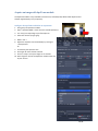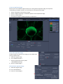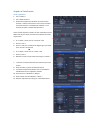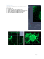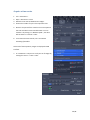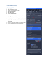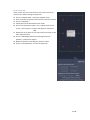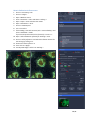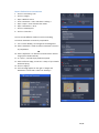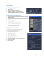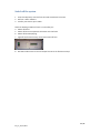
1
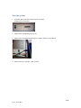
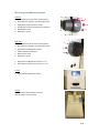
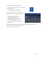
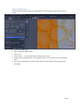
WIDEFIELD ZEISS AXIO OBSERVER
USER MANUAL
Start the system ...................................................................................................................................... 2
Equipment ............................................................................................................................................... 3
Microscope stand presentation .............................................................................................................. 4
Start Zen / Observation at oculars .......................................................................................................... 6
Acquire a widefield image in transmission mode with the color camera ............................................... 7
Acquisition in transmission ............................................................................................................. 7
Adjust the white balance ................................................................................................................. 8
Acquire a widefield image in fluorescence (and in BrightField) with the Black/White camera.............. 9
Acquire an image with ApoTome module ............................................................................................. 10
Configure the ApoTome and Make an Acquisition ....................................................................... 10
Create an ApoTome image ............................................................................................................ 11
Correct the ApoTome image ......................................................................................................... 11
Deconvoluate Apotome image ...................................................................................................... 11
Acquire a Z stack serie ........................................................................................................................... 12
Stack acquisition ............................................................................................................................ 12
Display the stack ............................................................................................................................ 13
Acquire a time serie............................................................................................................................... 14
Multiple stage positions ........................................................................................................................ 15
Acquire a mosaic image......................................................................................................................... 16
Tile scan acquisition ...................................................................................................................... 16
Focus correction ............................................................................................................................ 17
Mosaic finalization in fluorescence ............................................................................................... 18
Mosaic finalization in transmission ............................................................................................... 19
Graphic tools ......................................................................................................................................... 20
Save your data ....................................................................................................................................... 21
Save your experimental configuration .......................................................................................... 21
Save images with black and white camera .................................................................................... 21
Export images with color camera .................................................................................................. 21
Switch off the system ............................................................................................................................ 22
1 / 22
EV_V1_31/07/2014
Start the system
1. If needed, light on the fluorescence lamp on the desk.
It always has to be the first.
2. Switch on the multiple plug on your left.
3. Switch on the microscope by pushing the « START » button on the left side.
4. Switch on the PC, and log in « IJM » session.
2 / 22
EV_V1_31/07/2014
Equipment
Zeiss Axio Observer inverted motorized microscope + ApoTome Zeiss system
Black/White Axiocam MRm camera (pixel size 6.45*6.45 µm)
Axiocam HRc colour camera (pixel size 6.45*6.45 µm)
Motorized turntable in XY
Mercury vapor lamp with automatic alignment for fluorescence
Phase contrast and DIC
Filtres :
excitation
dichroic
emission
fluo
BP 335 - 383
BS 395
BP 420 - 470
DAPI
BP 424 - 448
BS 455
BP 460 - 500
CFP
BP 450 - 490
BS 495
BP 500 - 550
GFP
BP 538 - 562
BS 570
BP 570 - 640
DsRed
BP 625 - 655
BS 660
BP 665 - 715
CY5
Objectives :
Correction
NA
Working
distance
(mm)
coverslide
correction
(mm)
Immersion
medium
DIC
Phase
5x
Plan - Neofluar
0.15
4.8
0.17
Dry
No
No
10x
Plan - Neofluar
0.3
4.4
0.17
Dry
II
Ph1
25x
Plan - NeoFluar
0.8
0.57
0 - 017
Water, glycerol,
oil
II
40x
Plan-Apo
1.3
0.21
0.17
Oil
III
No
63x
Plan-Apo
1.4
0.19
0.17
Oil
III
No
100x
Plan-Apo
1.4
0.19
0.17
Oil
III
No
Objective
No
3 / 22
EV_V1_31/07/2014
Microscope stand presentation
Left side
1. Lower objectives turret at the lowest position
2. Reach back the objective at its working position
3. Open/Close the fluorescence shutter
4. Change filter cubes for fluorescence (2 buttons)
5. Macrometric screw
6. Micrometric screw
Right side
1. Lower objectives turret at the lowest position
2. Reach back the objective at its working position
3. Open/Close the BrightField shutter
4. Switch objectives (2 buttons)
5. Macrometric screw
6. Micrometric screw
4
3
6
2
5
1
4
3
2
6
5
1
7. Open/Close the BrightField shutter in « TL »
8. Open/Close the fluorescence shutter in « RL »
7
8
In front
1. Light intensity adjustment (wheel)
1
Joystick
Move the motorized turntable in X and Y.
Hold the button for moving fast.
4 / 22
TFT screen (touchscreen)
1. Open / Close the BrightField shutter
2. Open / Close the fluorescence shutter
In « Microscope » rubric, in « Control » menu, there are
several tabs allowing you to :
3. Choose the objective « Objectives »
4. Choose the filters cube for fluorescence
rescence « Reflector »
5. Add/retrieve a 1,5x lens « Optovar »
6. Observe in Fluorescence « FL »
7. Observe in Brightfield « BF »
8. Observe in phase contrast « PH »
9. Observe in Nomarski contrast « DIC »
5 / 22
Start Zen / Observation at oculars
1.
2.
3.
4.
Start « ZEN » software by clicking on the icon at the desktop.
Select « Locate » tab.
Click on « Ocular » to observe at oculars.
« TL » allows you to observe in transmission.
1
If you want to observe in phase contrast or in DIC, click on
« TL », then select « PH » or « DIC » on the TFT screen.
5.
6.
7.
8.
9.
10.
« DAPI » allows you to observe in blue.
« CFP » allows you to observe in cyan.
« GFP » allows you to observe in green.
« DsRed » allows you to observe in orange-red.
« Cy5 » allows you to observe in far red.
« Lights off » close the shutter in transmitted and
fluorescent light.
2
3
5
6
7
4
8
For transmitted light, phase contrast and Nomarski interference contrast (DIC) observation, it is really
important to make some adjustments at the microscope!
See panels post up in the microscope room.
6 / 22
10
9
Acquire a widefield image in transmission mode with the color camera
Acquisition in transmission
First of all, proceed to the Köhler alignment on the
microscope , before observing in brigtfield, phase contrast
or Nomarski contrast (see panels in the room).
1
Select « BF », « PH » or « DIC » on TFT screen.
2
1.
2.
3.
4.
5.
6.
Click on « Acquisition » tab.
Choose « TL - Camera couleur » mode.
Open « Channels » menu.
Tick « TL Brightfield » line.
Make « Live ».
Adjust the exposure time automatically by clicking on
« Set Exposure »
Or
7. Fix manually the exposure time.
8. Click on « Snap » to acquire an image.
5
8
3
4
7
6
7 / 22
Adjust the white balance
In a transmitted light image, adjust the « White Balance » allows to define a white reference of your
sample.
1
AVANT
3
2
6
4
5
APRES
1.
2.
3.
4.
5.
Go to « Acquisition » tab.
Open « Acquisition Mode » menu.
Make « Live ».
Click on « Pick. . . », a little stiletto appears instead of your arrow.
Choose a zone completely white in your image and click on. The correction is then automatically
done.
6. The « Auto » mode allows to correct the white balance, choose preferentially a region without
any sample.
8 / 22
Acquire a widefield image in fluorescence (and in BrightField) with
the Black/White camera
First of all, proceed to the Köhler alignment on the
microscope , before observing in brigtfield, phase contrast
or Nomarski contrast (see panels in the room).
1
Select « BF », « PH » or « DIC » on the TFT screen.
2
1.
2.
3.
4.
5.
6.
7.
Click on « Acquisition » tab.
Choose « Fluo + TL - Camera N&B » mode.
Open « Channels » menu.
Tick the line(s) corresponding to your fluorophores.
Select one channel (light gray).
Make « Live ».
Adjust the exposure time automatically by clicking on
« Set Exposure »
Or
8. Fix manually the exposure time.
9. Do it again for each channel selected.
10. Click on « Snap » to acquire images in all channels.
6
10
3
4
5
8
7
9 / 22
Acquire an image with ApoTome module
The Apotome module is only available in fluorescence, with 100X, 63X, 40X and 25X objectives and
without supplementary lens (no optovar).
Configure the ApoTome and Make an Acquisition
1. Push gently the ApoTome module.
2. Open « ApoTome Mode » menu and tick « Enable ApoTome ».
3. Tick line(s) corresponding to your fluorophores.
4. Select one channel (in light gray).
5. Make « Live ».
6. Adjust the exposure time automatically by clicking on
« Set Exposure »
Or
7. Fix manually the exposure time.
8. Do it again for each channel selected.
9. Click on « Snap » to acquire images in all channels.
10. Don't forget to retrieve the ApoTome module at the end
of your session.
1
5
9
2
4
3
7
6
10 / 22
Create an ApoTome image
Because of the intermediate images necessary for creating the final Apotome image, the acquisition
is demanding in computer memory. It is then better to only keep the final image :
1. Choose « ApoTome » tab below your image.
2. Choose « Optical sectioning » visualization options to see the ApoTome image.
3. Click on « Create Image ».
4. The ApoTome image is created and named « IP-ApoTome ».
4
1
2
3
Correct the ApoTome image
If ApoTome grid lines persist on the image, you can delete them
by using a Fourier filter.
5. Select the original image.
6. Tick « Enable correction ».
7. Choose and test Fourrier filter power
« Weak/Medium/Strong ».
8. Click on « Create Image ».
6
7
8
Deconvoluate Apotome image
9. Select the original image.
10. Tick « Deconvolution ».
11. Click on « Create Image ».
10
11 / 22
Acquire a Z stack serie
Stack acquisition
1. Tick « Z-Stack ».
2. Tick « Show all Tools ».
3. Choose the acquisition order when you have several
channels : make an entire stack in one color then switch
to the next channel « Full Z-Stack per Channel » or all
channels per plane « All Channels per Slices ».
2
There are two acquisition modes: the first one defines up and
down limits of your stack, the second one defines the center
of your stack.
5
1
4. In « Z-Stack » menu click on « First/Last » tab.
5. Click on « Live ».
6. Click on « Set First » to define the beginning of your stack
and « Set Last » for the end
OR
4. In « Z-Stack » menu click on « Center » tab.
5. Click on « Live ».
6. Define the center of your stack by clicking on « Center ».
7. « Interval » must be ticked to fix the value that you have
chosen.
8. Enter the value in µm for the desired interval.
9. To choose the optimal resolution click on the distance
indicated next to the « Optimal » mention.
10. The stack size is indicated in « Range ».
11. Slices number can be modified in « Slices ».
12. Start the acquisition by clicking on « Start Experiment ».
3
12
4
6
10
11
8
9
7
6
8
4
10
11
8
9
7
6
12 / 22
Display the stack
At the end of your acquisition, your stack is displayed at center of
ZEN interface.
In « Dimensions » tab:
13. To travel in the stack, move « Z--Position » cursor.
14. « Gallery » mode displays the set of images composing the stack.
15. « Ortho » mode allows an orthogonal view of your stack.
16. « 3D » mode allows a 3D visualization
visualiz
of your stack.
14
15
16
13
15
16
13 / 22
Acquire a time series
1.
2.
3.
4.
Tick « Time Series ».
Open « Time Series » menu.
Define the time interval between two images.
Choose the number of cycle or the acquisition time.
5. Remark : the period of the Z stack or tile scan acquisition
has to be included in time interval duration. You can
measure it by clicking on « Measure Speed », the value
will be shown in « Interval » rubric.
6. To minimize the time interval, tick « Use Camera
Streaming if Possible ».
1
At the end of the acquisition, images are displayed in ZEN
interface.
7. In « Dimensions » tab you can scroll your set of images by
moving the cursor in « Time » rubric.
2
4
3
6
5
7
14 / 22
Multiple stage positions
To make the software take into account the z coordinates for each position, you have to :
1. Open the « Focus Strategy » menu.
2. Choose « Local Focus Surface » option.
3. Choose « Fixed Z-position » option.
4.
5.
6.
7.
Tick « Tiles ».
Open « Tiles » menu.
Open « Positions » rubric.
Click on « Advanced Setup » to display the navigation space
where you will set your positions.
8. Click on « Live ».
9. Double click, on the navigation space where you want to
acquire an image or move thanks to the joystick.
10. Once positioned, click on the arrow next to « Positions » rubric.
Repeat this operation each time you want to save a position.
1
2
3
8
4
12
9
5
7
6
10
11
11. In « Single Positions » tab, you can see the coordinates list of all your positions that you have
saved.
12. Click on « Start Experiment ».
The multiposition option is also available on different type and size of multiple well-plates.
Seek advice from imaging facility engineers.
15 / 22
Acquire a mosaic image
Tile scan acquisition
1. Tick « Tiles ».
2. Open « Focus Strategy » menu.
3. Choose « Local Focus Surface » option.
4. Select « Fixed Z-position ».
5. Open « Tiles » menu.
6. Click on « Advanced Setup ».
7. Click on « Live ».
8. The navigation space is displayed in the center of the
software interface. Double-click on the desired position to
place the mosaic or move with the joystick.
9. In « Tile Regions » menu, click on « Tiles » and enter the size
1
of your mosaic. Your current position is the center of your
mosaic image.
10. Click on « + », the mosaic is drawn on the navigation space.
11. Click on « Star Experiment » to start the acquisition.
.
7
11
2
3
4
5
6
9
10
16 / 22
Focus correction
There are two ways to correct the focus on the entire mosaic. Be
careful to do it before starting the acquisition.
12. Click on « Support Points » below the navigation space.
13. Enter the number of positions where the focus will be corrected.
14. Click on « Distribute ».
15. Yellow points will be distributed on the mosaic.
16. Click on one yellow point, make « Live », adjust the focus and
click on « Set Current Z » to save it. Start again for each point.
OR
17. Double-click at the place on your mosaic where you want to save
the Z. Adjust the focus.
18. Click on « Add Support Point at Current Stage and Focus
position», a yellow point appears.
19. Repeat the process on five different positions at least.
20. Click on « Star Experiment » to start the acquisition.
15
18
12
16
13
14
18
17 / 22
Mosaic finalization in fluorescence
1. Click on « Processing » tab.
2. Click on « Single ».
3. Open « Method » menu.
4. Go to « Geometric » rubric and select « Stiching ».
5. Open « Input » menu and select the mosaic.
6. Open « Parameters » menu.
7. Click on « New Output ».
8. Tick « Fuse Tiles ».
9. If the shading is not well corrected, tick « Correct Shading » and
select « Automatic » mode.
If you have acquired several colors (channels) or a set in Z :
10. Open « Select dimension reference for stitching » menu.
11. Click on « All by reference » and select the referent channel for
the stiching by clicking on it.
12. Choose the referent plane in Z.
13. Then click on « Apply ».
14. The adjusted image is called « IP- Stitching ».
1
2
13
3
4
6
7
Avant
Après
8
9
10
11
12
5
18 / 22
Mosaic finalization in transmission
1. Click on « Processing » tab.
2. Click on « Single ».
3. Open « Method » menu.
4. Go to « Geometric » rubric and select « Stiching ».
5. Open « Input » menu and select the mosaic.
6. Open « Parameters » menu.
7. Click on « New Output ».
8. Click on « Fuse Tiles ».
1
2
13
3
You can use two different modes to correct the shading.
To make an automatic correction by computation :
9. Tick « Correct Shading » to homogenize the background.
10. Select « Automatic » mode to make an automatic correction
by computation.
OR
10. Select « Reference » to make the correction with a referent
image (more reliable method):
11. In « Input », a second empty window is opened
12. Select a referent image, it must be a « Snap » of your lamella
without anything.
13. Click on « Apply ».
14. The final image appears on the right in "Images and
Documents" column and is called « IP- Stitching ».
4
6
7
8
9
10
5
11
14
19 / 22
Graphic tools
In « Dimensions » tab
1. Display an image of one position in Z or in time by
entering its number or by moving the corresponding
cursor.
2. Adjust the image to the screen size.
3. Adjust image pixels size to the screen pixels size.
4. Enlarge or reduce the image.
5. Show/Hide a color (channel) on the screen.
6. See only one channel a time.
7. Show the gray level and the saturation.
In « Display » tab you can find contrast options.
8. Choose a color to modify or « All » to modify all of them.
9. Adjust automatically the contrast.
10. Reset the contrast.
1
2 3
4
5
6
7
8
10
9
In « Graphics » tab you can find annotation options.
11. Show the scale bar.
12. Show the time.
11
12
20 / 22
Save your data
Save your experimental configuration
1. Click on parameters logo.
2. Select « Save As ».
3. Rename your configuration and save it.
4. To load your parameters, open the menu below
« Experiment Manager » and select your configuration.
1
4
Save images with black and white camera
5. All images of your session are displayed on the right in « Images and
Documents » column.
6. To save, select the images by pressing Ctrl key and clicking on at the
same time.
7. Click on the little diskette.
8. Name your images.
9. Save them in the « Users » folder in J disk.
All images should be saved in this pathway :
J://users/year/month/day/your name.
Export images with color camera
You need to export data acquired with color camera
to open them with other software than ZEN.
10.
11.
12.
13.
14.
15.
16.
17.
18.
Click on File then Export or Ctrl+6.
« Parameters » tab opens.
Choose « TIFF » format.
Don't tick « Convert to 8 bit ».
Don't compress so tick « None ».
Tick « Original Data ».
Choose the export folder in the « Users » folder in J disk.
Untick « Create folder ».
Click on « Apply ».
5
6
7
11
12
13
14
15
16
17
21 / 22
Switch off the system
1. Lower the objectives, clean the front lens and around with lens tissue.
2. Exit from « ZEN » software.
3. Transfer your data on your hardisk.
Check the booking schedule. If there is no one after you :
4. Switch off the PC.
5. Switch off the microscope with the button on the left side.
6. Switch off the multiple plug.
7. Light off the fluorescent lamp. It has to be switch off last !
8. Put back the blue cover on the microscope but not on the fluorescent lamp!
22 / 22
EV_V1_31/07/2014