1
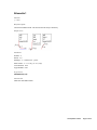
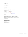
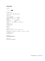
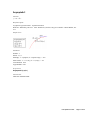
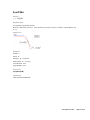
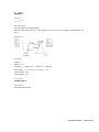
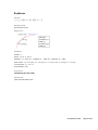
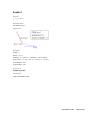
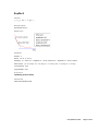
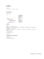
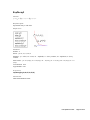
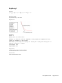
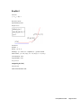
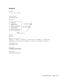
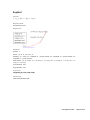
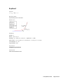
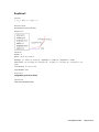
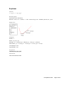
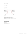
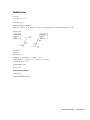
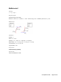
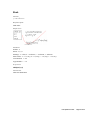
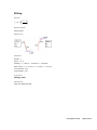
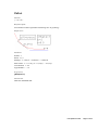
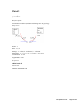
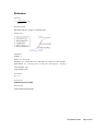
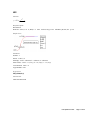
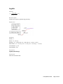
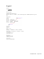
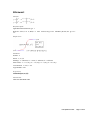
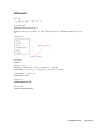
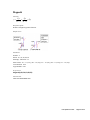
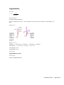
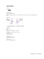
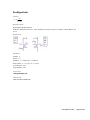
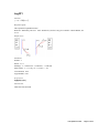
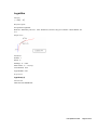
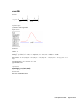
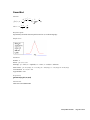
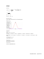
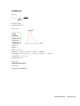
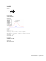
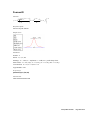
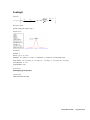
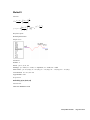
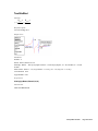
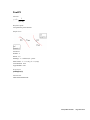
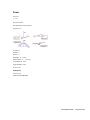
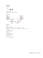
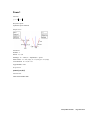
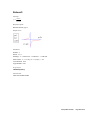
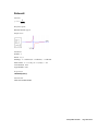
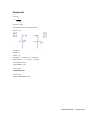
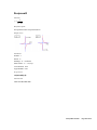
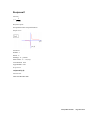
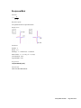
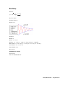
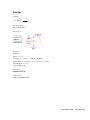
Curve Fitting Functions Contents 1. ORIGIN BASIC FUNCTIONS .......................................................................................................................... 2 2. CHROMATOGRAPHY FUNCTIONS ............................................................................................................... 23 3. EXPONENTIAL FUNCTIONS ........................................................................................................................ 30 4. GROWTH/SIGMOIDAL ................................................................................................................................ 69 5. HYPERBOLA FUNCTIONS ........................................................................................................................... 81 6. LOGARITHM FUNCTIONS ........................................................................................................................... 87 7. PEAK FUNCTIONS ...................................................................................................................................... 93 8. PHARMACOLOGY FUNCTIONS.................................................................................................................. 113 9. POWER FUNCTIONS ................................................................................................................................. 120 10. RATIONAL FUNCTIONS .......................................................................................................................... 140 11. SPECTROSCOPY FUNCTIONS .................................................................................................................. 155 12. WAVEFORM FUNCTIONS........................................................................................................................ 163 Last Updated 11/14/00 Page 1 of 166 1. Origin Basic Functions Allometric1 3 Beta 4 Boltzmann 5 Dhyperbl 6 ExpAssoc 7 ExpDecay1 8 ExpDecay2 9 ExpDecay3 10 ExpGrow1 11 ExpGrow2 12 Gauss 13 GaussAmp 14 Hyperbl 15 Logistic 16 LogNormal 17 Lorentz 18 Pulse 19 Rational0 20 Sine 21 Voigt 22 Last Updated 11/14/00 Page 2 of 166 Allometric1 Function y = ax b Brief Description Classical Freundlich model. Has been used in the study of allometry. Sample Curve Parameters Number: 2 Names: a, b Meanings: a = coefficient, b = power Initial Values: a = 1.0 (vary), b = 0.5 (vary) Lower Bounds: none Upper Bounds: none Script Access allometric1(x,a,b) Function File FITFUNC\ALLOMET1.FDF Last Updated 11/14/00 Page 3 of 166 Beta Function w + w3 − 2 x − xc y = y 0 + A1 + 2 w − 1 2 w1 w2 −1 w2 + w3 − 2 x − x c 1 − w − 1 3 w1 w3 −1 Brief Description The beta function. Sample Curve Parameters Number: 6 Names: y0, xc, A, w1, w2, w3 Meanings: y0 = offset, xc = center, A = amplitude, w1 = width, w2 = width, w3 = width Initial Values: y0 = 0.0 (vary), xc = 1.0 (vary), A = 5.0 (vary), w1 = 5.0 (vary), w2 = 2.0 (vary), w3 = 2.0 (vary) Lower Bounds: w1 > 0.0, w2 > 1.0, w3 > 1.0 Upper Bounds: none Script Access beta(x,y0,xc,A,w1,w2,w3) Function File FITFUNC\BETA.FDF Last Updated 11/14/00 Page 4 of 166 Boltzmann Function y= A1 − A2 + A2 1 + e ( x − x0 )/ dx Brief Description Boltzmann function - produces a sigmoidal curve. Sample Curve Parameters Number: 4 Names: A1, A2, x0, dx Meanings: A1 = initial value, A2 = final value, x0 = center, dx = time constant Initial Values: A1 = 0.0 (vary), A2 = 1.0 (vary), x0 = 0.0 (vary), dx = 1.0 (vary) Lower Bounds: none Upper Bounds: none Constraints dx ! = 0 Script Access boltzman(x,A1,A2,x0,dx) Function File FITFUNC\BOLTZMAN.FDF Last Updated 11/14/00 Page 5 of 166 Dhyperbl Function y= Px P1 x + 3 + P5 x P2 + x P4 + x Brief Description Double rectangular hyperbola function. Sample Curve Parameters Number: 5 Names: P1, P2, P3, P4, P5 Meanings: Unknowns 1-5 Initial Values: P1 = 1.0 (vary), P2 = 1.0 (vary), P3 = 1.0 (vary), P4 = 1.0 (vary), P5 = 1.0 (vary) Lower Bounds: none Upper Bounds: none Script Access dhyperbl(x,P1,P2,P3,P4,P5) Function File FITFUNC\DHYPERBL.FDF Last Updated 11/14/00 Page 6 of 166 ExpAssoc Function ( ) ( y = y0 + A1 1 − e − x / t1 + A2 1 − e − x / t2 ) Brief Description Exponential associate. Sample Curve Parameters Number: 5 Names: y0, A1, t1, A2, t2 Meanings: y0 = offset, A1 = amplitude, t1 = width, A2 = amplitude, t2 = width Initial Values: y0 = 0.0 (vary), A1 = 1.0 (vary), t1 = 1.0 (vary), A2 = 1.0 (vary), t2 = 1.0 (vary) Lower Bounds: t1 > 0, t2 > 0 Upper Bounds: none Script Access expassoc(x,y0,A1,t1,A2,t2) Function File FITFUNC\EXPASSOC.FDF Last Updated 11/14/00 Page 7 of 166 ExpDecay1 Function y = y0 + A1e − (x − x0 )/ t1 Brief Description Exponential decay 1 with offset. Sample Curve Parameters Number: 4 Names: y0, x0, A1, t1 Meanings: y0 = offset, x0 = center, A1 = amplitude, t1 = decay constant Initial Values: y0 = 0.0 (vary), x0 = 0.0 (vary), A1 = 10 (vary), t1 = 1.0 (vary) Lower Bounds: none Upper Bounds: none Script Access expdecay1(x,y0,x0,A1,t1) Function File FITFUNC\EXPDECY1.FDF Last Updated 11/14/00 Page 8 of 166 ExpDecay2 Function y = y0 + A1e − ( x− x0 )/ t1 + A2 e − (x − x0 )/ t2 Brief Description Exponential decay 2 with offset. Sample Curve Parameters Number: 6 Names: y0, x0, A1, t1, A2, t2 Meanings: y0 = offset, x0 = center, A1 = amplitude, t1 = decay constant, A2 = amplitude, t2 = decay constant Initial Values: y0 = 0.0 (vary), x0 = 0.0 (vary), A1 = 10 (vary), t1 = 1.0 (vary), A2 = 10 (vary), t2 = 1.0 (vary) Lower Bounds: none Upper Bounds: none Script Access expdecay2(x,y0,x0,A1,t1,A2,t2) Function File FITFUNC\EXPDECY2.FDF Last Updated 11/14/00 Page 9 of 166 ExpDecay3 Function y = y0 + A1e − ( x− x0 )/ t1 + A2 e − (x − x0 )/ t2 + A3e − (x − x0 )/ t3 Brief Description Exponential decay 3 with offset. Sample Curve Parameters Number: 8 Names: y0, x0, A1, t1, A2, t2, A3, t3 Meanings: y0 = offset, x0 = center, A1 = amplitude, t1 = decay constant, A2 = amplitude, t2 = decay constant, A3 = amplitude, t3 = decay constant Initial Values: y0 = 0.0 (vary), x0 = 0.0 (vary), A1 = 10 (vary), t1 = 1.0 (vary), A2 = 10 (vary), t2 = 1.0 (vary), A3 = 10 (vary), t3 = 1.0 (vary) Lower Bounds: none Upper Bounds: none Script Access expdecay3(x,y0,x0,A1,t1,A2,t2,A3,t3) Function File FITFUNC\EXPDECY3.FDF Last Updated 11/14/00 Page 10 of 166 ExpGrow1 Function y = y 0 + A1e ( x − x0 ) / t1 Brief Description Exponential growth 1 with offset. Sample Curve Parameters Number: 4 Names: y0, x0, A1, t1 Meanings: y0 = offset, x0 = center, A1 = amplitude, t1 = width Initial Values: y0 = 0.0 (vary), x0 = 0.0 (vary), A1 = 1.0 (vary), t1 = 1.0 (vary) Lower Bounds: t1 > 0.0 Upper Bounds: none Script Access expgrow1(x,y0,x0,A1,t1) Function File FITFUNC\EXPGROW1.FDF Last Updated 11/14/00 Page 11 of 166 ExpGrow2 Function y = y0 + A1e ( x− x0 )/ t1 + A2 e (x − x0 )/ t2 Brief Description Exponential growth 2 with offset. Sample Curve Parameters Number: 6 Names: y0, x0, A1, t1, A2, t2 Meanings: y0 = offset, x0 = center, A1 = amplitude, t1 = width, A2 = amplitude, t2 = width Initial Values: y0 = 0.0 (vary), x0 = 0.0 (vary), A1 = 1.0 (vary), t1 = 1.0 (vary), A2 = 1.0 (vary), t2 = 1.0 (vary) Lower Bounds: t1 > 0.0, t2 > 0.0 Upper Bounds: none Script Access expgrow2(x,y0,x0,A1,t1,A2,t2) Function File FITFUNC\EXPGROW2.FDF Last Updated 11/14/00 Page 12 of 166 Gauss Function −2 A y = y0 + e w π /2 ( x − xc )2 w2 Brief Description Area version of Gaussian function. Sample Curve Parameters Number: 4 Names: y0, xc, w, A Meanings: y0 = offset, xc = center, w = width, A = area Initial Values: y0 = 0.0 (vary), xc = 0.0 (vary), w = 1.0 (vary), A = 10 (vary) Lower Bounds: w > 0.0 Upper Bounds: none Script Access gauss(x,y0,xc,w,A) Function File FITFUNC\GAUSS.FDF Last Updated 11/14/00 Page 13 of 166 GaussAmp Function y = y0 + Ae − ( x − xc )2 2 w2 Brief Description Amplitude version of Gaussian peak function. Sample Curve Parameters Number: 4 Names: y0, xc, w, A Meanings: y0 = offset, xc = center, w = width, A = area Initial Values: y0 = 0.0 (vary), xc = 0.0 (vary), w = 1.0 (vary), A = 10 (vary) Lower Bounds: w > 0.0 Upper Bounds: none Script Access gaussamp(x,y0,xc,w,A) Function File FITFUNC\GAUSSAMP.FDF Last Updated 11/14/00 Page 14 of 166 Hyperbl Function y= P1 x P2 + x Brief Description Hyperbola function. Also the Michaelis-Menten model in enzyme kinetics. Sample Curve Parameters Number: 2 Names: P1, P2 Meanings: P1 = amplitude, P2 = unknown Initial Values: P1 = 1.0 (vary), P2 = 1.0 (vary) Lower Bounds: none Upper Bounds: none Script Access hyperbl(x,P1,P2) Function File FITFUNC\HYPERBL.FDF Last Updated 11/14/00 Page 15 of 166 Logistic Function y= A1 − A2 + A2 p 1 + (x / x0 ) Brief Description Logistic dose response in pharmacology/chemistry. Sample Curve Parameters Number: 4 Names: A1, A2, x0, p Meanings: A1 = initial value, A2 = final value, x0 = center, p = power Initial Values: A1 = 0.0 (vary), A2 = 1.0 (vary), x0 = 1.0 (vary), p = 1.5 (vary) Lower Bounds: p > 0.0 Upper Bounds: none Script Access logistic(x,A1,A2,x0,p) Function File FITFUNC\LOGISTIC.FDF Last Updated 11/14/00 Page 16 of 166 LogNormal Function y = y0 + A 2π wx −[ln x / xc ]2 e 2 w2 Brief Description Log-Normal function. Sample Curve Parameters Number: 4 Names: y0, xc, w, A Meanings: y0 = offset, xc = center, w = width, A = amplitude Initial Values: y0 = 0.0 (vary), xc = 1.0 (vary), w = 1.0 (vary), A = 1.0 (vary) Lower Bounds: xc > 0, w > 0 Upper Bounds: none Script Access lognormal(x,y0,xc,w,A) Function File FITFUNC\LOGNORM.FDF Last Updated 11/14/00 Page 17 of 166 Lorentz Function y = y0 + 2A w π 4(x − xc )2 + w 2 Brief Description Lorentzian peak function. Sample Curve Parameters Number: 4 Names: y0, xc, w, A Meanings: y0 = offset, xc = center, w = width, A = area Initial Values: y0 = 0.0 (vary), xc = 0.0 (vary),w = 1.0 (vary), A = 1.0 (vary) Lower Bounds: w > 0.0 Upper Bounds: none Script Access lorentz(x,y0,xc,w,A) Function File FITFUNC\LORENTZ.FDF Last Updated 11/14/00 Page 18 of 166 Pulse Function p x − x0 − − x −t x0 t1 y = y0 + A 1 − e e 2 Brief Description Pulse function. Sample Curve Parameters Number: 6 Names: y0, x0, A, t1, P, t2 Meanings: y0 = offset, x0 = center, A = amplitude, t1 = width, P = power, t2 = width Initial Values: y0 = 0.0 (vary), x0 = 0.0 (vary), A = 1.0 (vary), t1 = 1.0 (vary), P = 1.0 (vary), t2 = 1.0 (vary) Lower Bounds: A > 0.0, t1 > 0.0, P > 0.0, t2 > 0.0 Upper Bounds: none Script Access pulse(x,y0,x0,A,t1,P,t2) Function File FITFUNC/PULSE.FDF Last Updated 11/14/00 Page 19 of 166 Rational0 Function y= b + cx 1 + ax Brief Description Rational function, type 0. Reference: Ratkowksy, David A. 1990. Handbook of Nonlinear Regression Models. Marcel Dekker, Inc. 4.3.24 Sample Curve Parameters Number: 3 Names: a, b, c Meanings: a = coefficient, b = coefficient, c = coefficient Initial Values: a = 1.0 (vary), b = 1.0 (vary), c = 0.5 Lower Bounds: none Upper Bounds: none Script Access rational0(x,a,b,c) Function File FITFUNC\RATION0.FDF Last Updated 11/14/00 Page 20 of 166 Sine Function x − xc y = A sin π w Brief Description Sine function. Sample Curve Parameters Number: 3 Names: xc, w, A Meanings: xc = center, w = width, A = amplitude Initial Values: xc = 0.0 (vary), w = 1.0 (vary), A = 1.0 (vary) Lower Bounds: w > 0.0 Upper Bounds: none Script Access sine(x,xc,w,A) Function File FITFUNC\SINE.FDF Last Updated 11/14/00 Page 21 of 166 Voigt Function 2 ln 2 wL ∞ e −t ⋅ dt 2 2 π 3 / 2 wG2 ∫−∞ wL x − xc ln 2 + 4 ln 2 − t wG wG 2 y = y0 + A ⋅ Brief Description Voigt peak function. Sample Curve Parameters Number: 5 Names: y0, xc, A, wG, wL Meanings: y0 = offset, xc = center, A = amplitude, wG = Gaussian width, wL = Lorentzian width Initial Values: y0 = 0.0 (vary), xc = 0.0 (vary), A = 1.0 (vary), wG = 1.0 (vary), wL = 1.0 (vary) Lower Bounds: wG > 0.0, wL > 0.0 Upper Bounds: none Script Access voigt5(x,y0,xc,A,wG,wL) Function File FITFUNC\VOIGT5.FDF Last Updated 11/14/00 Page 22 of 166 2. Chromatography Functions CCE 24 ECS 25 Gauss 26 GaussMod 27 GCAS 28 Giddings 29 Last Updated 11/14/00 Page 23 of 166 CCE Function − ( x − xc 1 ) −0.5 k ( x − x + ( x − xc 3 )) y = y0 + Ae 2 w + B(1 − 0.5(1 − tanh (k 2 (x − xc ))))e 3 c 3 2 Brief Description Chesler-Cram peak function for use in chromatography. Sample Curve Parameters Number: 9 Names: y0, xc1, A, w, k2, xc2, B, k3, xc3 Meanings: y0 = offset, xc1 = unknown, A = unknown, w = unknown, k2 = unknown, xc2 = unknown, B = unknown, k3 = unknown, xc3 = unknown Initial Values: y0 = 0.0 (vary), xc1 = 1.0 (vary), A = 1.0 (vary), w = 1.0 (vary), k2 = 1.0 (vary), xc2 = 1.0 (vary), B = 1.0 (vary), k3 = 1.0 (vary), xc3 = 1.0 (vary) Lower Bounds: w > 0.0 Upper Bounds: none Script Access cce(x,y0,xc1,A,w,k2,xc2,B,k3,xc3) Function File FITFUNC\CHESLECR.FDF Last Updated 11/14/00 Page 24 of 166 ECS Function a 4 a3 2 3 1 + z z − 3 + 4 z − 6 z + 3 A −0.5 z 2 3! 4! y = y0 + e 2 10a3 6 w 2π 4 2 z − 15 z + 45 z − 15 + 6! ( ) ( ( where z= ) ) x − xc w Brief Description Edgeworth-Cramer peak function for use in chromatography. Sample Curve Parameters Number: 6 Names: y0, xc, A, w, a3, a4 Meanings: y0 = offset, xc = center, A = amplitude, w = width, a3 = unknown, a4 = unknown Initial Values: y0 = 0.0 (vary), xc = 0.0 (vary), A = 1.0 (vary), w = 1.0 (vary), a3 = 1.0 (vary), a4 = 1.0 (vary) Lower Bounds: A > 0.0, w > 0.0 Upper Bounds: none Script Access ecs(x,y0,xc,A,w,a3,a4) Function File FITFUNC\EDGWTHCR.FDF Last Updated 11/14/00 Page 25 of 166 Gauss Function −2 A y = y0 + e w π /2 ( x − xc )2 w2 Brief Description Area version of Gaussian function. Sample Curve Parameters Number: 4 Names: y0, xc, w, A Meanings: y0 = offset, xc = center, w = width, A = area Initial Values: y0 = 0.0 (vary), xc = 0.0 (vary), w = 1.0 (vary), A = 10 (vary) Lower Bounds: w > 0.0 Upper Bounds: none Script Access gauss(x,y0,xc,w,A) Function File FITFUNC\GAUSS.FDF Last Updated 11/14/00 Page 26 of 166 GaussMod Function 1 w A 2 t f ( x) = y0 + e 0 t0 where z= 2 − x − xc t0 ∫ z −∞ y2 1 −2 e dy 2π x − xc w − w t0 Brief Description Exponentially modified Gaussian peak function for use in chromatography. Sample Curve Parameters Number: 5 Names: y0, A, xc, w, t0 Meanings: y0 = offset, A = amplitude, xc = center, w = width, t0 = unknown Initial Values: y0 = 0.0 (vary), A = 1.0 (vary), xc = 0.0 (vary), w = 1.0 (vary), t0 = 0.05 (vary) Lower Bounds: w > 0.0, t0 > 0.0 Upper Bounds: none Script Access gaussmod(x,y0,A,xc,w,t0) Function File FITFUNC\GAUSSMOD.FDF Last Updated 11/14/00 Page 27 of 166 GCAS Function f ( z ) = y0 + 4 2 a A e − z / 2 1 + ∑ i H i (z ) w 2π i =3 i! x − xc w H 3 = z 3 − 3z z= H 4 = z 4 − 6z 3 + 3 Brief Description Gram-Charlier peak function for use in chromatography. Sample Curve Parameters Number: 6 Names: y0, xc, A, w, a3, a4 Meanings: y0 = offset, xc = center, A = amplitude, w = width, a3 = unknown, a4 = unknown Initial Values: y0 = 0.0 (vary), xc = 0.0 (vary), A = 1.0 (vary), w = 1.0 (vary), a3 = 0.01 (vary), a4 = 0.001 (vary) Lower Bounds: w > 0.0 Upper Bounds: none Script Access gcas(x,y0,xc,A,w,a3,a4) Function File FITFUNC\GRMCHARL.FDF Last Updated 11/14/00 Page 28 of 166 Giddings Function y = y0 + A w − x− x xc 2 xc x w c I1 e x w Brief Description Giddings peak function for use in chromatography. Sample Curve Parameters Number: 4 Names: y0, xc, w, A Meanings: y0 = offset, xc = center, w = width, A = area Initial Values: y0 = 0.0 (vary), xc = 1.0 (vary), w = 1.0 (vary), A = 1.0 (vary) Lower Bounds: w > 0.0 Upper Bounds: none Script Access giddings(x,y0,xc,w,A) Function File FITFUNC\GIDDINGS.FDF Last Updated 11/14/00 Page 29 of 166 3. Exponential Functions Asymtotic1 31 BoxLucas1 32 BoxLucas1Mod 33 BoxLucas2 34 Chapman 35 Exp1P1 36 Exp1P2 37 Exp1P2md 38 Exp1P3 39 Exp1P3Md 40 Exp1P4 41 Exp1P4Md 42 Exp2P 43 Exp2PMod1 44 Exp2PMod2 45 Exp3P1 46 Exp3P1Md 47 Exp3P2 48 ExpAssoc 49 ExpDec1 50 ExpDec2 51 ExpDec3 52 ExpDecay1 53 ExpDecay2 54 ExpDecay3 55 ExpGro1 56 ExpGro2 57 ExpGro3 58 ExpGrow1 59 ExpGrow2 60 ExpLinear 61 Exponential 62 MnMolecular 63 MnMolecular1 64 Shah 65 Stirling 66 YldFert 67 YldFert1 68 Last Updated 11/14/00 Page 30 of 166 Asymptotic1 Function y = a − bc x Brief Description Asymptotic regression model - 1st parameterization. Reference: Ratkowksy, David A. 1990. Handbook of Nonlinear Regression Models. Marcel Dekker, Inc. 4.3.1 Sample Curve Parameters Number: 3 Names: a, b, c Meanings: a = asymptote, b = response range, c = rate Initial Values: a = 1.0 (vary), b = 1.0 (vary), c = 0.5 Lower Bounds: none Upper Bounds: none Script Access Asymptotic1(x,a,b,c) Function File FITFUNC\ASYMPT1.FDF Last Updated 11/14/00 Page 31 of 166 BoxLucas1 Function ( y = a 1 − e − bx ) Brief Description A parameterization of Box Lucas model. Sample Curve Parameters Number: 2 Names: a, b Meanings: a = coefficient, b = coefficient Initial Values: a = 1.0 (vary), b = 1.0 (vary) Lower Bounds: none Upper Bounds: none Script Access boxlucas1(x,a,b) Function File FITFUNC\BOXLUC1.FDF Last Updated 11/14/00 Page 32 of 166 BoxLucas1Mod Function ( y = a 1− bx ) Brief Description A parameterization of Box Lucas model. Reference: Ratkowksy, David A. 1990. Handbook of Nonlinear Regression Models. Marcel Dekker, Inc. 4.3.5 Sample Curve Parameters Number: 2 Names: a, b Meanings: a = coefficient, b = coefficient Initial Values: a = 1.0 (vary), b = 1.0 (vary) Lower Bounds: none Upper Bounds: none Script Access boxlucas1mod(x,a,b) Function File FITFUNC\BOXLC1MD.FDF Last Updated 11/14/00 Page 33 of 166 BoxLucas2 Function y= ( a1 e − a2 x − e − a1x a1 − a2 ) Brief Description A parameterization of Box Lucas model. Reference: Seber, G. A. F., Wild, C. J. 1989. Nonlinear Regression. John Wiley & Sons, Inc. p. 254 Sample Curve Parameters Number: 2 Names: a1, a2 Meanings: a1 = unknown, a2 = unknown Initial Values: a1 = 2.0 (vary), a2 = 1.0 (vary) Lower Bounds: none Upper Bounds: none Script Access boxlucas2(x,a1,a2) Function File FITFUNC\BOXLUC2.FDF Last Updated 11/14/00 Page 34 of 166 Chapman Function ( y = a 1 − e − bx ) c Brief Description Chapman model. Reference: Ratkowksy, David A. 1990. Handbook of Nonlinear Regression Models. Marcel Dekker, Inc. 4.3.35 Sample Curve Parameters Number: 3 Names: a, b, c Meanings: a = coefficient, b = coefficient, c = coefficient Initial Values: a = 1.0 (vary), b = 1.0 (vary), c = 0.5 Lower Bounds: none Upper Bounds: none Script Access chapman(x,a,b,c) Function File FITFUNC\CHAPMAN.FDF Last Updated 11/14/00 Page 35 of 166 Exp1P1 Function y = e x− A Brief Description One-parameter exponential function. Reference: Ratkowksy, David A. 1990. Handbook of Nonlinear Regression Models. Marcel Dekker, Inc. 4.1.5 Sample Curve y(1)=1 position:A=1 (A,1) y=0 Parameters Number: 1 Names: A Meanings: A = position Initial Values: A = 1.0 (vary) Lower Bounds: none Upper Bounds: none Script Access exp1p1(x,A) Function File FITFUNC\EXP1P1.FDF Last Updated 11/14/00 Page 36 of 166 Exp1p2 Function y = e − Ax Brief Description One-parameter exponential function. Reference: Ratkowksy, David A. 1990. Handbook of Nonlinear Regression Models. Marcel Dekker, Inc. 4.1.15 Sample Curve Parameters Number: 1 Names: A Meanings: A = coefficient Initial Values: A = 1.0 (vary) Lower Bounds: none Upper Bounds: none Script Access exp1p2(x,A) Function File FITFUNC\EXP1P2.FDF Last Updated 11/14/00 Page 37 of 166 Exp1p2md Function y = Bx Brief Description One-parameter exponential function. Reference: Ratkowksy, David A. 1990. Handbook of Nonlinear Regression Models. Marcel Dekker, Inc. 4.1.16 Sample Curve Parameters Number: 1 Names: B Meanings: B = position Initial Values: B = 1.0 (vary) Lower Bounds: none Upper Bounds: none Script Access exp1p2md(x,B) Function File FITFUNC\EXP1P2MD.FDF Last Updated 11/14/00 Page 38 of 166 Exp1p3 Function y = Ae − Ax Brief Description One-parameter exponential function. Reference: Ratkowksy, David A. 1990. Handbook of Nonlinear Regression Models. Marcel Dekker, Inc. 4.1.13 Sample Curve Parameters Number: 1 Names: A Meanings: A = coefficient Initial Values: A = 1.0 (vary) Lower Bounds: none Upper Bounds: none Script Access exp1p3(x,A) Function File FITFUNC\EXP1P3.FDF Last Updated 11/14/00 Page 39 of 166 Exp1P3Md Function y = − ln (B )B x Brief Description One-parameter exponential function. Reference: Ratkowksy, David A. 1990. Handbook of Nonlinear Regression Models. Marcel Dekker, Inc. 4.1.14 Sample Curve Parameters Number: 1 Names: B Meanings: B = coefficient Initial Values: B = 5.0 (vary) Lower Bounds: none Upper Bounds: none Script Access exp1p3md(x,B) Function File FITFUNC\EXP1P3MD.DFD Last Updated 11/14/00 Page 40 of 166 Exp1P4 Function y = 1 − e − Ax Brief Description One-parameter exponential function. Reference: Ratkowksy, David A. 1990. Handbook of Nonlinear Regression Models. Marcel Dekker, Inc. 4.1.18 Sample Curve Parameters Number: 1 Names: A Meanings: A = coefficient Initial Values: A = 1.0 (vary) Lower Bounds: none Upper Bounds: none Script Access exp1p4(x,A) Function File FITFUNC\EXP1P4.FDF Last Updated 11/14/00 Page 41 of 166 Exp1P4Md Function y = 1− Bx Brief Description One-parameter exponential function. Reference: Ratkowksy, David A. 1990. Handbook of Nonlinear Regression Models. Marcel Dekker, Inc. 4.1.19 Sample Curve Parameters Number: 1 Names: B Meanings: B = coefficient Initial Values: B = 1.0 (vary) Lower Bounds: none Upper Bounds: none Script Access exp1p4md(x,B) Function File FITFUNC\EXP1P4.FDF Last Updated 11/14/00 Page 42 of 166 Exp2P Function y = ab x Brief Description Two-parameter exponential function. Reference: Ratkowksy, David A. 1990. Handbook of Nonlinear Regression Models. Marcel Dekker, Inc. 4.2.9 Sample Curve Parameters Number: 2 Names: a, b Meanings: a = position, b = position Initial Values: a = 1.0 (vary), b = 1.5 (vary) Lower Bounds: none Upper Bounds: none Script Access exp2p(x,a,b) Function File FITFUNC\EXP2P.FDF Last Updated 11/14/00 Page 43 of 166 Exp2PMod1 Function y = ae bx Brief Description Two-parameter exponential function. Reference: Ratkowksy, David A. 1990. Handbook of Nonlinear Regression Models. Marcel Dekker, Inc. 4.2.10 Sample Curve Parameters Number: 2 Names: a, b Meanings: a = coefficient, b = rate Initial Values: a = 1.0 (vary), b = 1.5 (vary) Lower Bounds: none Upper Bounds: none Script Access exp2pmod1(x,a,b) Function File FITFUNC\EXP2PMD1.FDF Last Updated 11/14/00 Page 44 of 166 Exp2PMod2 Function y = e a+bx Brief Description Two-parameter exponential function. Reference: Ratkowksy, David A. 1990. Handbook of Nonlinear Regression Models. Marcel Dekker, Inc. 4.2.11 Sample Curve Parameters Number: 2 Names: a, b Meanings: a = coefficient, b = rate Initial Values: a = 1.0 (vary), b =1.5 (vary) Lower Bounds: none Upper Bounds: none Script Access exp2pmod2(x,a,b) Function File FITFUNC\EXP2PMD2.FDF Last Updated 11/14/00 Page 45 of 166 Exp3P1 Function y = ae b x+c Brief Description Three-parameter exponential function. Reference: Ratkowksy, David A. 1990. Handbook of Nonlinear Regression Models. Marcel Dekker, Inc. 4.3.33 Sample Curve Parameters Number: 3 Names: a, b, c Meanings: a = coefficient, b = coefficient, c = coefficient Initial Values: a = 1.0 (vary), b = 1.0 (vary), c = 0.5 Lower Bounds: none Upper Bounds: none Script Access exp3p1(x,a,b,c) Function File FITFUNC\EXP3P1.FDF Last Updated 11/14/00 Page 46 of 166 Exp3P1Md Function y=e a+ b x+c Brief Description Three-parameter exponential function. Reference: Ratkowksy, David A. 1990. Handbook of Nonlinear Regression Models. Marcel Dekker, Inc. 4.3.34 Sample Curve Parameters Number: 3 Names: a, b, c Meanings: a = coefficient, b = coefficient, c = coefficient Initial Values: a = 1.0 (vary), b = 1.0 (vary), c = 0.5 Lower Bounds: none Upper Bounds: none Script Access exp3p1md(x,a,b,c) Function File FITFUNC\EXP3P1MD.FDF Last Updated 11/14/00 Page 47 of 166 Exp3P2 Function y = e a +bx +cx 2 Brief Description Three-parameter exponential function. Reference: Ratkowksy, David A. 1990. Handbook of Nonlinear Regression Models. Marcel Dekker, Inc. 4.3.39 Sample Curve Parameters Number: 3 Names: a, b, c Meanings: a = coefficient, b = coefficient, c = coefficient Initial Values: a = 1.0 (vary), b = 1.0 (vary), c = 0.5 Lower Bounds: none Upper Bounds: none Script Access exp3p2(x,a,b,c) Function File FITFUNC\EXP3P2.FDF Last Updated 11/14/00 Page 48 of 166 ExpAssoc Function ( ) ( y = y0 + A1 1 − e − x / t1 + A2 1 − e − x / t2 ) Brief Description Exponential associate. Sample Curve Parameters Number: 5 Names: y0, A1, t1, A2, t2 Meanings: y0 = offset, A1 = amplitude, t1 = width, A2 = amplitude, t2 = width Initial Values: y0 = 0.0 (vary), A1 = 1.0 (vary), t1 = 1.0 (vary), A2 = 1.0 (vary), t2 = 1.0 (vary) Lower Bounds: t1 > 0, t2 > 0 Upper Bounds: none Script Access expassoc(x,y0,A1,t1,A2,t2) Function File FITFUNC\EXPASSOC.FDF Last Updated 11/14/00 Page 49 of 166 ExpDec1 Function y = y0 + Ae − x / t Brief Description Exponential decay 1. Sample Curve Parameters Number: 3 Names: y0, A, t Meanings: y0 = offset, A = amplitude, t = decay constant Initial Values: y0 = 0.0 (vary), A = 1.0 (vary), t = 1.0 (vary) Lower Bounds: none Upper Bounds: none Script Access expdec1(x,y0,A,t) Function File FITFUNC\EXPDEC1.FDF Last Updated 11/14/00 Page 50 of 166 ExpDec2 Function y = y0 + A1e − x / t1 + A2 e − x / t2 Brief Description Exponential decay 2. Sample Curve Parameters Number: 5 Names: y0, A1, t1, A2, t2 Meanings: y0 = offset, A1 = amplitude, t1 = decay constant, A2 = amplitude, t2 = decay constant Initial Values: y0 = 0.0 (vary), A1 = 1.0 (vary), t1 = 1.0 (vary), A2 = 1.0 (vary), t2 = 1.0 (vary) Lower Bounds: none Upper Bounds: none Script Access expdec2(x,y0,A1,t1,A2,t2) Function File FITFUNC\EXPDEC2.FDF Last Updated 11/14/00 Page 51 of 166 ExpDec3 Function y = y0 + A1e − x / t1 + A2 e − x / t2 + A3 e − x / t3 Brief Description Exponential decay 3. Sample Curve Parameters Number: 7 Names: y0, A1, t1, A2, t2, A3, t3 Meanings: y0 = offset, A1 = amplitude, t1 = decay constant, A2 = amplitude, t2 = decay constant, A3 = amplitude, t3 = decay constant Initial Values: y0 = 0.0 (vary), A1 = 1.0 (vary), t1 = 1.0 (vary), A2 = 1.0 (vary), t2 = 1.0 (vary), A3 = 1.0 (vary), t3 = 1.0 (vary) Lower Bounds: none Upper Bounds: none Script Access expdec3(x,y0,A1,t1,A2,t2,A3,t3) Function File FITFUNC\EXPDEC3.FDF Last Updated 11/14/00 Page 52 of 166 ExpDecay1 Function y = y0 + A1e − (x − x0 )/ t1 Brief Description Exponential decay 1 with offset. Sample Curve Parameters Number: 4 Names: y0, x0, A1, t1 Meanings: y0 = offset, x0 = center, A1 = amplitude, t1 = decay constant Initial Values: y0 = 0.0 (vary), x0 = 0.0 (vary), A1 = 10 (vary), t1 = 1.0 (vary) Lower Bounds: none Upper Bounds: none Script Access expdecay1(x,y0,x0,A1,t1) Function File FITFUNC\EXPDECY1.FDF Last Updated 11/14/00 Page 53 of 166 ExpDecay2 Function y = y0 + A1e − ( x− x0 )/ t1 + A2 e − (x − x0 )/ t2 Brief Description Exponential decay 2 with offset. Sample Curve Parameters Number: 6 Names: y0, x0, A1, t1, A2, t2 Meanings: y0 = offset, x0 = center, A1 = amplitude, t1 = decay constant, A2 = amplitude, t2 = decay constant Initial Values: y0 = 0.0 (vary), x0 = 0.0 (vary), A1 = 10 (vary), t1 = 1.0 (vary), A2 = 10 (vary), t2 = 1.0 (vary) Lower Bounds: none Upper Bounds: none Script Access expdecay2(x,y0,x0,A1,t1,A2,t2) Function File FITFUNC\EXPDECY2.FDF Last Updated 11/14/00 Page 54 of 166 ExpDecay3 Function y = y0 + A1e − ( x− x0 )/ t1 + A2 e − (x − x0 )/ t2 + A3e − (x − x0 )/ t3 Brief Description Exponential decay 3 with offset. Sample Curve Parameters Number: 8 Names: y0, x0, A1, t1, A2, t2, A3, t3 Meanings: y0 = offset, x0 = center, A1 = amplitude, t1 = decay constant, A2 = amplitude, t2 = decay constant, A3 = amplitude, t3 = decay constant Initial Values: y0 = 0.0 (vary), x0 = 0.0 (vary), A1 = 10 (vary), t1 = 1.0 (vary), A2 = 10 (vary), t2 = 1.0 (vary), A3 = 10 (vary), t3 = 1.0 (vary) Lower Bounds: none Upper Bounds: none Script Access expdecay3(x,y0,x0,A1,t1,A2,t2,A3,t3) Function File FITFUNC\EXPDECY3.FDF Last Updated 11/14/00 Page 55 of 166 ExpGro1 Function y = y 0 + A1e x / t1 Brief Description Exponential growth 1. Sample Curve Parameters Number: 3 Names: y0, A1, t1 Meanings: y0 = offset, A1 = amplitude, t1 = growth constant Initial Values: y0 = 0.0 (vary), A1 = 1.0 (vary), t1 = 1.0 (vary) Lower Bounds: none Upper Bounds: none Script Access expgro1(x,y0,A1,t1) Function File FITFUNC\EXPGRO1.FDF Last Updated 11/14/00 Page 56 of 166 ExpGro2 Function y = y0 + A1e x / t1 + A2 e x / t2 Brief Description Exponential growth 2. Sample Curve Parameters Number: 5 Names: y0, A1, t1, A2, t2 Meanings: y0 = offset, A1 = amplitude, t1 = growth constant, A2 = amplitude, t2 = growth constant Initial Values: y0 = 0.0 (vary), A1 = 1.0 (vary), t1 = 1.0 (vary), A2 = 1.0 (vary), t2 = 1.0 (vary) Lower Bounds: none Upper Bounds: none Script Access expgro2(x,y0,A1,t1,A2,t2) Function File FITFUNC\EXPGRO2.FDF Last Updated 11/14/00 Page 57 of 166 ExpGro3 Function y = y0 + A1e x / t1 + A2 e x / t2 + A3e x / t3 Brief Description Exponential growth 3. Sample Curve Parameters Number: 7 Names: y0, A1, t1, A2, t2, A3, t3 Meanings: y0 = offset, A1 = amplitude, t1 = growth constant, A2 = amplitude, t2 = growth constant, A3 = amplitude, t3 = growth constant Initial Values: y0 = 0.0 (vary), A1 = 1.0 (vary), t1 = 1.0 (vary), A2 = 1.0 (vary), t2 = 1.0 (vary), A3 = 1.0 (vary), t3 = 1.0 (vary) Lower Bounds: none Upper Bounds: none Script Access expgro3(x,y0,A1,t1,A2,t2,A3,t3) Function File FITFUNC\EXPGRO3.FDF Last Updated 11/14/00 Page 58 of 166 ExpGrow1 Function y = y 0 + A1e ( x − x0 ) / t1 Brief Description Exponential growth 1 with offset. Sample Curve Parameters Number: 4 Names: y0, x0, A1, t1 Meanings: y0 = offset, x0 = center, A1 = amplitude, t1 = width Initial Values: y0 = 0.0 (vary), x0 = 0.0 (vary),A1 = 1.0 (vary), t1 = 1.0 (vary) Lower Bounds: t1 > 0.0 Upper Bounds: none Script Access expgrow1(x,y0,x0,A1,t1) Function File FITFUNC\EXPGROW1.FDF Last Updated 11/14/00 Page 59 of 166 ExpGrow2 Function y = y0 + A1e ( x− x0 )/ t1 + A2 e (x − x0 )/ t2 Brief Description Exponential growth 2 with offset. Sample Curve Parameters Number: 6 Names: y0, x0, A1, t1, A2, t2 Meanings: y0 = offset, x0 = center, A1 = amplitude, t1 = width, A2 = amplitude, t2 = width Initial Values: y0 = 0.0 (vary), x0 = 0.0 (vary), A1 = 1.0 (vary), t1 = 1.0 (vary), A2 = 1.0 (vary), t2 = 1.0 (vary) Lower Bounds: t1 > 0.0, t2 > 0.0 Upper Bounds: none Script Access expgrow2(x,y0,x0,A1,t1,A2,t2) Function File FITFUNC\EXPGROW2.FDF Last Updated 11/14/00 Page 60 of 166 ExpLinear Function y = p1e − x / p2 + p3 + p 4 x Brief Description Exponential linear combination. Reference: Seber, G. A. F., Wild, C. J. 1989. Nonlinear Regression. John Wiley & Sons, Inc. p. 298 Sample Curve Parameters Number: 4 Names: p1, p2, p3, p4 Meanings: p1 = coefficient, p2 = unknown, p3 = offset, p4 = coefficient Initial Values: p1 = 1.0 (vary), p2 = 1.0 (vary), p3 = 1.0 (vary), p4 = 1.0 (vary) Lower Bounds: none Upper Bounds: none Script Access explinear(x,p1,p2,p3,p4) Function File FITFUNC\EXPLINEA.FDF Last Updated 11/14/00 Page 61 of 166 Exponential Function y = y0 + Ae R0 x Brief Description Exponential. Sample Curve Parameters Number: 3 Names: y0, A, R0 Meanings: y0 = offset, A = initial value, R0 = rate Initial Values: y0 = 0.0 (vary), A = 1.0 (vary), R0 = 1.0 (vary) Lower Bounds: A > 0.0 Upper Bounds: none Script Access exponential(x,y0,A,R0) Function File FITFUNC\EXPONENT.FDF Last Updated 11/14/00 Page 62 of 166 MnMolecular Function ( y = A 1 − e − k ( x− xc ) ) Brief Description Monomolecular growth model. Reference: Seber, G. A. F., Wild, C. J. 1989. Nonlinear Regression. John Wiley & Sons, Inc. p. 328 Sample Curve Parameters Number: 3 Names: A, xc, k Meanings: A = amplitude, xc = center, k = rate Initial Values: A = 2.0 (vary), xc = 1.0 (vary), k = 1.0 (vary) Lower Bounds: A > 0.0 Upper Bounds: none Script Access mnmolecular(x,A,xc,k) Function File FITFUNC\MMOLECU.FDF Last Updated 11/14/00 Page 63 of 166 MnMolecular1 Function y = A1 − A2 e − kx Brief Description Monomolecular growth model. Reference: Seber, G. A. F., Wild, C. J. 1989. Nonlinear Regression. John Wiley & Sons, Inc. p. 328 Sample Curve Parameters Number: 3 Names: A1, A2, k Meanings: A1 = offset, A2 = coefficient, k = coefficient Initial Values: A1 = 1.0 (vary), A2 = 1.0 (vary), k = 1.0 (vary) Lower Bounds: A1 > 0.0, A2 > 0.0 Upper Bounds: none Script Access mnmolecular1(x,A1,A2,k) Function File FITFUNC\MMOLECU1.FDF Last Updated 11/14/00 Page 64 of 166 Shah Function y = a + bx + cr x Brief Description Shah model. Sample Curve Parameters Number: 4 Names: a, b, c, r Meanings: a = offset, b = coefficient, c = coefficient, r = unknown Initial Values: a = 1.0 (vary), b = 1.0 (vary), c = 1.0 (vary), r = 0.5 (vary) Lower Bounds: r > 0.0 Upper Bounds: r < 1.0 Script Access shah(x,a,b,c,r) Function File FITFUNC\SHAH.FDF Last Updated 11/14/00 Page 65 of 166 Stirling Function e kx − 1 y = a + b k Brief Description Stirling model. Sample Curve Parameters Number: 3 Names: a, b, k Meanings: a = offset, b = coefficient, k = coefficient Initial Values: a = 1.0 (vary), b = 1.0 (vary), k = 1.0 (vary) Lower Bounds: none Upper Bounds: none Script Access stirling(x,a,b,k) Function File FITFUNC\STIRLING.FDF Last Updated 11/14/00 Page 66 of 166 YldFert Function y = a + br x Brief Description Yield-fertilizer model in agriculture and learning curve in psychology. Sample Curve Parameters Number: 3 Names: a, b, r Meanings: a = offset, b = coefficient, r = coefficient Initial Values: a = 1.0 (vary), b = 1.0 (vary), r = 0.5 (vary) Lower Bounds: r > 0.0 Upper Bounds: r < 1.0 Script Access yldfert(x,a,b,r) Function File FITFUNC\YLDFERT.FDF Last Updated 11/14/00 Page 67 of 166 YldFert1 Function y = a + be − kx Brief Description Yield-fertilizer model in agriculture and learning curve in psychology. Sample Curve Parameters Number: 3 Names: a, b, k Meanings: a = offset, b = coefficient, k = coefficient Initial Values: a = 1.0 (vary), b = 1.0 (vary), k = 0.5 (vary) Lower Bounds: k > 0.0 Upper Bounds: none Script Access yldfert1(x,a,b,k) Function File FITFUNC\YLDFERT1.FDF Last Updated 11/14/00 Page 68 of 166 4. Growth/Sigmoidal Boltzmann 70 Hill 71 Logistic 72 SGompertz 73 SLogistic1 74 SLogistic2 75 SLogistic3 76 SRichards1 77 SRichards2 78 SWeibull1 79 SWeibull2 80 Last Updated 11/14/00 Page 69 of 166 Boltzmann Function y= A1 − A2 + A2 1 + e ( x − x0 )/ dx Brief Description Boltzmann function - produces a sigmoidal curve. Sample Curve Parameters Number: 4 Names: A1, A2, x0, dx Meanings: A1 = initial value, A2 = final value, x0 = center, dx = time constant Initial Values: A1 = 0.0 (vary), A2 = 1.0 (vary), x0 = 0.0 (vary), dx = 1.0 (vary) Lower Bounds: none Upper Bounds: none Constraints dx ! = 0 Script Access boltzman(x,A1,A2,x0,dx) Function File FITFUNC\BOLTZMAN.FDF Last Updated 11/14/00 Page 70 of 166 Hill Function y = Vmax xn k n + xn Brief Description Hill function. Reference: Seber, G. A. F., Wild, C. J. 1989. Nonlinear Regression. John Wiley & Sons, Inc. p. 120 Sample Curve Parameters Number: 3 Names: Vmax, k, n Meanings: Vmax = unknown, k = unknown, n = unknown Initial Values: Vmax = 1.0 (vary), k = 1.0 (vary), n = 1.5 (vary) Lower Bounds: Vmax > 0 Upper Bounds: none Script Access hill(x,Vmax,k,n) Function File FITFUNC\HILL.FDF Last Updated 11/14/00 Page 71 of 166 Logistic Function y= A1 − A2 + A2 p 1 + (x / x0 ) Brief Description Logistic dose response in pharmacology/chemistry. Sample Curve Parameters Number: 4 Names: A1, A2, x0, p Meanings: A1 = initial value, A2 = final value, x0 = center, p =power Initial Values: A1 = 0.0 (vary), A2 = 1.0 (vary), x0 = 1.0 (vary), p = 1.5 (vary) Lower Bounds: p > 0.0 Upper Bounds: none Script Access logistic(x,A1,A2,x0,p) Function File FITFUNC\LOGISTIC.FDF Last Updated 11/14/00 Page 72 of 166 SGompertz Function y = ae − exp (− k (x − xc )) Brief Description Gompertz growth model for population studies, animal growth. Reference: Seber, G. A. F., Wild, C. J. 1989. Nonlinear Regression. John Wiley & Sons, Inc. pp. 330 331 Sample Curve Parameters Number: 3 Names: a, xc, k Meanings: a = amplitude, xc = center, k = coefficient Initial Values: a = 1.0 (vary), xc = 1.0 (vary), k = 1.0 (vary) Lower Bounds: a > 0.0, k > 0.0 Upper Bounds: none Script Access sgompertz(x,a,xc,k) Function File FITFUNC\GOMPERTZ.FDF Last Updated 11/14/00 Page 73 of 166 SLogistic1 Function y= a 1+ e − k ( x − xc ) Brief Description Sigmoidal logistic function, type 1. Reference: Seber, G. A. F., Wild, C. J. 1989. Nonlinear Regression. John Wiley & Sons, Inc. pp. 328 330 Sample Curve Parameters Number: 3 Names: a, xc, k Meanings: a = amplitude, xc = center, k = coefficient Initial Values: a = 1.0 (vary), xc = 1.0 (vary), k = 1.0 (vary) Lower Bounds: xc > 0 Upper Bounds: none Script Access slogistic1(x,a,xc,k) Function File FITFUNC\SLOGIST1.FDF Last Updated 11/14/00 Page 74 of 166 SLogistic2 Function y= a 1+ a − y0 −4Wmax x / a e y0 Brief Description Sigmoidal logistic function, type 2. Reference: Seber, G. A. F., Wild, C. J. 1989. Nonlinear Regression. John Wiley & Sons, Inc. pp. 328 330 Sample Curve Parameters Number: 3 Names: y0, a, Wmax Meanings: y0 = initial value, a = amplitude, Wmax = maximum growth rate Initial Values: y0 = 0.5 (vary), a = 1.0 (vary), Wmax = 1.0 (vary) Lower Bounds: y0 > 0.0, a > 0.0, Wmax > 0.0 Upper Bounds: none Script Access slogistic2(x,y0,a,Wmax) Function File FITFUNC\SLOGIST2.FDF Last Updated 11/14/00 Page 75 of 166 SLogistic3 Function y= a 1 + be −kx Brief Description Sigmoidal logistic function, type 3. Reference: Seber, G. A. F., Wild, C. J. 1989. Nonlinear Regression. John Wiley & Sons, Inc. pp. 328 330 Sample Curve Parameters Number: 3 Names: a, b, k Meanings: a = amplitude, b = coefficient, k = coefficient Initial Values: a = 1.0 (vary), b = 1.0 (vary), k = 1.0 (vary) Lower Bounds: a > 0.0, b > 0.0, k >0.0 Upper Bounds: none Script Access slogistic3(x,a,b,k) Function File FITFUNC\SLOGIST3.FDF Last Updated 11/14/00 Page 76 of 166 SRichards1 Function [ y = [a ]( ) ( ] y = a1−d − e −k (x − xc ) 1− d + e − k ( x − xc 1 / 1− d ) 1 / 1− d ) ,d <1 ,d >1 Brief Description Sigmoidal Richards function, type 1. Reference: Seber, G. A. F., Wild, C. J. 1989. Nonlinear Regression. John Wiley & Sons, Inc. pp. 332 337 Sample Curve Parameters Number: 4 Names: a, xc, d, k Meanings: a = unknown, xc = center, d = unknown, k = coefficient Initial Values: a = 1.0 (vary), xc = 1.0 (vary), d = 5 (vary), k = 0.5 (vary) Lower Bounds: a > 0.0, k > 0.0 Upper Bounds: none Script Access srichards1(x,a,xc,d,k) Function File FITFUNC\SRICHAR1.FDF Last Updated 11/14/00 Page 77 of 166 SRichards2 Function [ y = a 1 + (d − 1)e −k ( x− xc ) ]( 1 / 1− d ) ,d ≠1 Brief Description Sigmoidal Richards function, type 2. Reference: Seber, G. A. F., Wild, C. J. 1989. Nonlinear Regression. John Wiley & Sons, Inc. pp. 332 337 Sample Curve Parameters Number: 4 Names: a, xc, d, k Meanings: a = unknown, xc = center, d = unknown, k = coefficient Initial Values: a = 1.0 (vary), xc = 1.0 (vary), d = 5.0 (vary), k = 1.0 (vary) Lower Bounds: a > 0.0, k > 0.0 Upper Bounds: none Script Access srichards2(x,a,xc,d,k) Function File FITFUNC\SRICHAR2.FDF Last Updated 11/14/00 Page 78 of 166 SWeibull1 Function ( y = A 1 − e −(k (x − xc )) d ) Brief Description Sigmoidal Weibull function, type 1. Reference: Seber, G. A. F., Wild, C. J. 1989. Nonlinear Regression. John Wiley & Sons, Inc. pp. 338 339 Sample Curve Parameters Number: 4 Names: A, xc, d, k Meanings: A = amplitude, xc = center, d = power, k = coefficient Initial Values: A = 1.0 (vary), xc = 1.0 (vary), d = 5.0 (vary), k = 1.0 (vary) Lower Bounds: A > 0.0, k > 0.0 Upper Bounds: none Script Access sweibull1(x,A,xc,d,k) Function File FITFUNC\WEIBULL1.FDF Last Updated 11/14/00 Page 79 of 166 SWeibull2 Function y = A − (A − B )e − (kx ) d Brief Description Sigmoidal Weibull function, type 2. Reference: Seber, G. A. F., Wild, C. J. 1989. Nonlinear Regression. John Wiley & Sons, Inc. pp. 338 339 Sample Curve Parameters Number: 4 Names: a, b, d, k Meanings: a = unknown, b = unknown, d = power, k = coefficient Initial Values: a = 1.0 (vary), b = 1.0 (vary), d = 5.0 (vary), k = 1.0 (vary) Lower Bounds: a > 0.0, b > 0.0, k > 0.0 Upper Bounds: none Script Access sweibull2(x,a,b,d,k) Function File FITFUNC\WEIBULL2.FDF Last Updated 11/14/00 Page 80 of 166 5. Hyperbola Functions Dhyperbl 82 Hyperbl 83 HyperbolaGen 84 HyperbolaMod 85 RectHyperbola 86 Last Updated 11/14/00 Page 81 of 166 Dhyperbl Function y= Px P1 x + 3 + P5 x P2 + x P4 + x Brief Description Double rectangular hyperbola function. Sample Curve Parameters Number: 5 Names: P1, P2, P3, P4, P5 Meanings: Unknowns 1-5 Initial Values: P1 = 1.0 (vary), P2 = 1.0 (vary), P3 = 1.0 (vary), P4 = 1.0 (vary), P5 = 1.0 (vary) Lower Bounds: none Upper Bounds: none Script Access dhyperbl(x,P1,P2,P3,P4,P5) Function File FITFUNC\DHYPERBL.FDF Last Updated 11/14/00 Page 82 of 166 Hyperbl Function y= P1 x P2 + x Brief Description Hyperbola function. Also the Michaelis-Menten model in enzyme kinetics. Sample Curve Parameters Number: 2 Names: P1, P2 Meanings: P1 = amplitude, P2 = unknown Initial Values: P1 = 1.0 (vary), P2 = 1.0 (vary) Lower Bounds: none Upper Bounds: none Script Access hyperbl(x,P1,P2) Function File FITFUNC\HYPERBL.FDF Last Updated 11/14/00 Page 83 of 166 HyperbolaGen Function y=a− b (1 + cx )1 / d Brief Description Generalized hyperbola function. Reference: Ratkowksy, David A. 1990. Handbook of Nonlinear Regression Models. Marcel Dekker, Inc. 4.4.7 Sample Curve Parameters Number: 4 Names: a, b, c, d Meanings: a = coefficient, b = coefficient, c = coefficient, d = coefficient Initial Values: a = 1.0 (vary), b = 1.0 (vary), c = 0.5, d = 0.5 Lower Bounds: none Upper Bounds: none Script Access hyperbolagen(x,a,b,c,d) Function File FITFUNC\HYPERGEN.FDF Last Updated 11/14/00 Page 84 of 166 HyperbolaMod Function y= x θ1 x + θ 2 Brief Description Modified hyperbola function. Reference: Ratkowksy, David A. 1990. Handbook of Nonlinear Regression Models. Marcel Dekker, Inc. 4.2.18 Sample Curve Parameters Number: 2 Names: T1, T2 Meanings: T1 = amplitude, T2 = unknown Initial Values: T1 = 1.0 (vary), T2 = 1.0 (vary) Lower Bounds: none Upper Bounds: none Script Access hyperbolamod(x,T1,T2) Function File FITFUNC\HYPERBMD.FDF Last Updated 11/14/00 Page 85 of 166 RectHyperbola Function y=a bx 1 + bx Brief Description Rectangular hyperbola function. Reference: Ratkowksy, David A. 1990. Handbook of Nonlinear Regression Models. Marcel Dekker, Inc. 4.2.16 Sample Curve Parameters Number: 2 Names: a, b Meanings: a = coefficient, b = coefficient Initial Values: a = 1.0 (vary), b = 1.0 (vary) Lower Bounds: none Upper Bounds: none Script Access recthyperbola(x,a,b) Function File FITFUNC\RECTHYPB.FDF Last Updated 11/14/00 Page 86 of 166 6. Logarithm Functions Bradley 88 Log2P1 89 Log2P2 90 Log3P1 91 Logarithm 92 Last Updated 11/14/00 Page 87 of 166 Bradley Function y = a ln (− b ln( x) ) Brief Description Bradley model. Reference: Ratkowksy, David A. 1990. Handbook of Nonlinear Regression Models. Marcel Dekker, Inc. 3.3.7 Sample Curve Parameters Number: 2 Names: a, b Meanings: a = unknown, b = unknown Initial Values: a = 1.0 (vary), b = 1.0 (vary) Lower Bounds: none Upper Bounds: none Script Access bradley(x,a,b) Function File FITFUNC\BRADLEY.FDF Last Updated 11/14/00 Page 88 of 166 Log2P1 Function y = b ln (x − a ) Brief Description Two-parameter logarithm function. Reference: Ratkowksy, David A. 1990. Handbook of Nonlinear Regression Models. Marcel Dekker, Inc. 4.2.1 Sample Curve Parameters Number: 2 Names: a, b Meanings: a = offset, b = coefficient Initial Values: a = 1.0 (vary), b = 1.0 (vary) Lower Bounds: none Upper Bounds: none Script Access log2p1(x,a,b) Function File FITFUNC\LOG2P1.FDF Last Updated 11/14/00 Page 89 of 166 Log2P2 Function y = ln(a + bx ) Brief Description Two-parameter logarithm. Reference: Ratkowksy, David A. 1990. Handbook of Nonlinear Regression Models. Marcel Dekker, Inc. 4.2.3 Sample Curve Parameters Number: 2 Names: a, b Meanings: a = offset, b = coefficient Initial Values: a = 1.0 (vary), b = 1.0 (vary) Lower Bounds: none Upper Bounds: none Script Access log2p2(x,a,b) Function File FITFUNC\LOG2P2.FDF Last Updated 11/14/00 Page 90 of 166 Log3P1 Function y = a − b ln (x + c ) Brief Description Three-parameter logarithm function. Reference: Ratkowksy, David A. 1990. Handbook of Nonlinear Regression Models. Marcel Dekker, Inc. 4.3.32 Sample Curve Parameters Number: 3 Names: a, b, c Meanings: a = coefficient, b = coefficient, c = coefficient Initial Values: a = 1.0 (vary), b = 1.0 (vary), c = 0.5 Lower Bounds: none Upper Bounds: none Script Access log3p1(x,a,b,c) Function File FITFUNC\LOG3P1.FDF Last Updated 11/14/00 Page 91 of 166 Logarithm Function y = ln (x − A) Brief Description One-parameter logarithm. Reference: Ratkowksy, David A. 1990. Handbook of Nonlinear Regression Models. Marcel Dekker, Inc. 4.1.1 Sample Curve Parameters Number: 1 Names: A Meanings: A = center Initial Values: A = 1.0 (vary) Lower Bounds: none Upper Bounds: none Script Access logarithm(x,A) Function File FITFUNC\LOGARITH.FDF Last Updated 11/14/00 Page 92 of 166 7. Peak Functions Asym2Sig 94 Beta 95 CCE 96 ECS 97 Extreme 98 Gauss 99 GaussAmp 100 GaussMod 101 GCAS 102 Giddings 103 InvsPoly 104 LogNormal 105 Logistpk 106 Lorentz 107 PearsonVII 108 PsdVoigt1 109 PsdVoigt2 110 Voigt 111 Weibull3 112 Last Updated 11/14/00 Page 93 of 166 Asym2Sig Function 1 y = y0 + A 1+ e − x − xc + w1 / 2 w2 1 1 − x − xc − w1 / 2 − w3 1+ e Brief Description Asymmetric double sigmoidal. Sample Curve Parameters Number: 6 Names: y0, xc, A, w1, w2, w3 Meanings: y0 = offset, xc = center, A = amplitude, w1 = width, w2 = width, w3 = width Initial Values: y0 = 0.0 (vary), xc = 0.0 (vary), A = 1.0 (vary), w1 = 1.0 (vary), w2 = 1.0 (vary), w3 = 1.0 (vary) Lower Bounds: w1 > 0.0, w2 > 0.0, w3 > 0.0 Upper Bounds: none Script Access asym2sig(x,y0,xc,A,w1,w2,w3) Function File FITFUNC\ASYMDBLS.FDF Last Updated 11/14/00 Page 94 of 166 Beta Function w + w3 − 2 x − xc y = y 0 + A1 + 2 w − 1 2 w1 w2 −1 w2 + w3 − 2 x − x c 1 − w − 1 3 w1 w3 −1 Brief Description The beta function. Sample Curve Parameters Number: 6 Names: y0, xc, A, w1, w2, w3 Meanings: y0 = offset, xc = center, A = amplitude, w1 = width, w2 = width, w3 = width Initial Values: y0 = 0.0 (vary), xc = 1.0 (vary), A = 5.0 (vary), w1 = 5.0 (vary), w2 = 2.0 (vary), w3 = 2.0 (vary) Lower Bounds: w1 > 0.0, w2 > 1.0, w3 > 1.0 Upper Bounds: none Script Access beta(x,y0,xc,A,w1,w2,w3) Function File FITFUNC\BETA.FDF Last Updated 11/14/00 Page 95 of 166 CCE Function − ( x − xc 1 ) 0.5 k ( x − x + ( x − xc 3 )) y = y 0 + Ae 2 w + B(1 − 0.5(1 − tanh (k 2 (x − xC 2 ))))e 3 c 3 2 Brief Description Chesler-Cram peak function for use in chromatography. Sample Curve Parameters Number: 9 Names: y0, xc1, A, w, k2, xc2, B, k3, xc3 Meanings: y0 = offset, xc1 = unknown, A = unknown, w = unknown, k2 = unknown, xc2 = unknown, B = unknown, k3 = unknown, xc3 = unknown Initial Values: y0 = 0.0 (vary), xc1 = 1.0 (vary), A = 1.0 (vary), w = 1.0 (vary), k2 = 1.0 (vary), xc2 = 1.0 (vary), B = 1.0 (vary), k3 = 1.0 (vary), xc3 = 1.0 (vary) Lower Bounds: w > 0.0 Upper Bounds: none Script Access cce(x,y0,xc1,A,w,k2,xc2,B,k3,xc3) Function File FITFUNC\CHESLECR.FDF Last Updated 11/14/00 Page 96 of 166 ECS Function a 4 a3 2 3 1 + z z − 3 + 4 z − 6 z + 3 A −0.5 z 2 3! 4! y = y0 + e 2 10a3 6 w 2π 4 2 z − 15 z + 45 z − 15 + 6! ( ) ( ( where z= ) ) x − xc w Brief Description Edgeworth-Cramer peak function for use in chromatography. Sample Curve Parameters Number: 6 Names: y0, xc, A, w, a3, a4 Meanings: y0 = offset, xc = center, A = amplitude, w = width, a3 = unknown, a4 = unknown Initial Values: y0 = 0.0 (vary), xc = 0.0 (vary), A = 1.0 (vary), w = 1.0 (vary), a3 = 1.0 (vary), a4 = 1.0 (vary) Lower Bounds: A > 0.0, w > 0.0 Upper Bounds: none Script Access ecs(x,y0,xc,A,w,a3,a4) Function File FITFUNC\EDGWTHCR.FDF Last Updated 11/14/00 Page 97 of 166 Extreme Function x − xc x − xc y = y0 + Ae − exp − − + 1 w w Brief Description Extreme function in statistics. Sample Curve Parameters Number: 4 Names: y0, xc, w, A Meanings: y0 = offset, xc = center, w = width, A = amplitude Initial Values: y0 = 0.0 (vary), xc = 1.0 (vary), w = 1.0 (vary), A = 1.0 (vary) Lower Bounds: w > 0.0 Upper Bounds: none Script Access extreme(x,y0,xc,w,A) Function File FITFUNC\EXTREME.FDF Last Updated 11/14/00 Page 98 of 166 Gauss Function −2 A y = y0 + e w π /2 ( x − xc )2 w2 Brief Description Area version of Gaussian function. Sample Curve Parameters Number: 4 Names: y0, xc, w, A Meanings: y0 = offset, xc = center, w = width, A = area Initial Values: y0 = 0.0 (vary), xc = 0.0 (vary), w = 1.0 (vary), A = 10 (vary) Lower Bounds: w > 0.0 Upper Bounds: none Script Access gauss(x,y0,xc,w,A) Function File FITFUNC\GAUSS.FDF Last Updated 11/14/00 Page 99 of 166 GaussAmp Function y = y0 + Ae − ( x − xc )2 2 w2 Brief Description Amplitude version of Gaussian peak function. Sample Curve Parameters Number: 4 Names: y0, xc, w, A Meanings: y0 = offset, xc = center, w = width, A = area Initial Values: y0 = 0.0 (vary), xc = 0.0 (vary), w = 1.0 (vary), A = 10 (vary) Lower Bounds: w > 0.0 Upper Bounds: none Script Access gaussamp(x,y0,xc,w,A) Function File FITFUNC\GAUSSAMP.FDF Last Updated 11/14/00 Page 100 of 166 GaussMod Function 1 w A 2 t f ( x) = y0 + e 0 t0 where z= 2 − x − xc t0 ∫ z −∞ y2 1 −2 e dy 2π x − xc w − w t0 Brief Description Exponentially modified Gaussian peak function for use in chromatography. Sample Curve Parameters Number: 5 Names: y0, A, xc, w, t0 Meanings: y0 = offset, A = amplitude, xc = center, w = width, t0 = unknown Initial Values: y0 = 0.0 (vary), A = 1.0 (vary), xc = 0.0 (vary), w = 1.0 (vary), t0 = 0.05 (vary) Lower Bounds: w > 0.0, t0 > 0.0 Upper Bounds: none Script Access gaussmod(x,y0,A,xc,w,t0) Function File FITFUNC\GAUSSMOD.FDF Last Updated 11/14/00 Page 101 of 166 GCAS Function f ( z ) = y0 + 4 2 a A e − z / 2 1 + ∑ i H i (z ) w 2π i =3 i! x − xc w H 3 = z 3 − 3z z= H 4 = z 4 − 6z 3 + 3 Brief Description Gram-Charlier peak function for use in chromatography. Sample Curve Parameters Number: 6 Names: y0, xc, A, w, a3, a4 Meanings: y0 = offset, xc = center, A = amplitude, w = width, a3 = unknown, a4 = unknown Initial Values: y0 = 0.0 (vary), xc = 0.0 (vary), A = 1.0 (vary), w = 1.0 (vary), a3 = 0.01 (vary), a4 = 0.001 (vary) Lower Bounds: w > 0.0 Upper Bounds: none Script Access gcas(x,y0,xc,A,w,a3,a4) Function File FITFUNC\GRMCHARL.FDF Last Updated 11/14/00 Page 102 of 166 Giddings Function y = y0 + A w − x− x xc 2 xc x w c I1 e x w Brief Description Giddings peak function for use in chromatography. Sample Curve Parameters Number: 4 Names: y0, xc, w, A Meanings: y0 = offset, xc = center, w = width, A = area Initial Values: y0 = 0.0 (vary), xc = 1.0 (vary), w = 1.0 (vary), A = 1.0 (vary) Lower Bounds: w > 0.0 Upper Bounds: none Script Access giddings(x,y0,xc,w,A) Function File FITFUNC\GIDDINGS.FDF Last Updated 11/14/00 Page 103 of 166 InvsPoly Function y = y0 + A x − xc x − xc x − xc 1 + A1 2 + A2 2 + A3 2 w w w 2 4 6 Brief Description Inverse polynomial peak function with center. Sample Curve Parameters Number: 7 Names: y0, xc, w, A, A1, A2, A3 Meanings: y0 = offset, xc = center, w = width, A = amplitude, A1 = coefficient, A2 = coefficient, A3 = coefficient Initial Values: y0 = 0.0 (vary), xc = 0.0 (vary), w = 1.0 (vary), A = 1.0 (vary), A1 = 0.0 (vary), A2 = 0.0 (vary), A3 = 0.0 (vary) Lower Bounds: w > 0.0, A1 ≥ 0.0, A2 ≥ 0.0, A3 ≥ 0.0 Upper Bounds: none Script Access invspoly(x,y0,xc,w,A,A1,A2,A3) Function File FITFUNC\INVSPOLY.FDF Last Updated 11/14/00 Page 104 of 166 LogNormal Function y = y0 + A 2π wx −[ln x / xc ]2 e 2 w2 Brief Description Log-Normal function. Sample Curve Parameters Number: 4 Names: y0, xc, w, A Meanings: y0 = offset, xc = center, w = width, A = amplitude Initial Values: y0 = 0.0 (vary), xc = 1.0 (vary), w = 1.0 (vary), A = 1.0 (vary) Lower Bounds: xc > 0, w > 0 Upper Bounds: none Script Access lognormal(x,y0,xc,w,A) Function File FITFUNC\LOGNORM.FDF Last Updated 11/14/00 Page 105 of 166 Logistpk Function y = y0 + 4 Ae − x − xc w x − xc − 1 + e w 2 Brief Description Logistic peak function. Sample Curve Parameters Number: 4 Names: y0, xc, w, A Meanings: y0 = offset, xc = center, w = width, A = amplitude Initial Values: y0 = 0.0 (vary), xc = 1.0 (vary), w = 1.0 (vary), A = 1.0 (vary) Lower Bounds: w > 0.0 Upper Bounds: none Script Access logistpk(x,y0,xc,w,A) Function File FITFUNC\LOGISTPK Last Updated 11/14/00 Page 106 of 166 Lorentz Function y = y0 + 2A w π 4(x − xc )2 + w 2 Brief Description Lorentzian peak function. Sample Curve Parameters Number: 4 Names: y0, xc, w, A Meanings: y0 = offset, xc = center, w = width, A = area Initial Values: y0 = 0.0 (vary), xc = 0.0 (vary), w = 1.0 (vary), A = 1.0 (vary) Lower Bounds: w > 0.0 Upper Bounds: none Script Access lorentz(x,y0,xc,w,A) Function File FITFUNC\LORENTZ.FDF Last Updated 11/14/00 Page 107 of 166 PearsonVII Function 1 / mu − mu 2 mu e (Γ ( 2 −1) ) 21 / mu − 1 2 (x − xc ) y=A 1 + 4 π e (Γ ( mu −1 / 2) ) w2 Brief Description Pearson VII peak function. Sample Curve Parameters Number: 4 Names: xc, A, w, mu Meanings: xc = center, A = amplitude, w = width, mu = profile shape factor Initial Values: xc = 0.0 (vary), A = 1.0 (vary), w = 1.0 (vary), mu = 1.0 (vary) Lower Bounds: A > 0.0, w > 0.0, mu > 0.0 Upper Bounds: none Script Access pearson7(x,xc,A,w,mu) Function File FITFUNC\PEARSON7.FDF Last Updated 11/14/00 Page 108 of 166 PsdVoigt1 Function 4 ln 2 2 w 4 ln 2 − w2 ( x − xc )2 y = y0 + Amu e + (1 − mu ) 2 2 πw π 4(x − xc ) + w Brief Description Pseudo-Voigt peak function type 1. Sample Curve Parameters Number: 5 Names: y0, xc, A, w, mu Meanings: y0 = offset, xc = center, A = amplitude, w = width, mu = profile shape factor Initial Values: y0 = 0.0 (vary), xc = 0.0 (vary), A = 1.0 (vary), w = 1.0 (vary), mu = 0.5 (vary) Lower Bounds: w > 0.0 Upper Bounds: none Script Access psdvoigt1(x,y0,xc,A,w,mu) Function File FITFUNC\PSDVGT1.FDF Last Updated 11/14/00 Page 109 of 166 PsdVoigt2 Function 4 ln 2 2 wL 2 4 ln 2 − wG 2 ( x − xc ) ( ) y = y 0 + Am u m e 1 + − u 2 2 π wG π 4(x − x c ) + wL Brief Description Pseudo-Voigt peak function type 2. Sample Curve Parameters Number: 6 Names: y0, xc, A, wG, wL, mu Meanings: y0 = offset, xc = center, A = amplitude, wG = width, wL = width, mu = profile shape factor Initial Values: y0 = 0.0 (vary), xc = 0.0 (vary), A = 1.0 (vary), wG = 1.0 (vary), wL = 1.0 (vary), mu = 0.5 (vary) Lower Bounds: wG > 0.0, wL > 0.0 Upper Bounds: none Script Access psdvoigt2(x,y0,xc,A,wG,wL,mu) Function File FITFUNC\PSDVGT2.FDF Last Updated 11/14/00 Page 110 of 166 Voigt Function 2 ln 2 wL ∞ e −t ⋅ dt 2 2 π 3 / 2 wG2 ∫−∞ wL x − xc ln 2 + 4 ln 2 − t wG wG 2 y = y0 + A ⋅ Brief Description Voigt peak function. Sample Curve Parameters Number: 5 Names: y0, xc, A, wG, wL Meanings: y0 = offset, xc = center, A = amplitude, wG = Gaussian width, wL = Lorentzian width Initial Values: y0 = 0.0 (vary), xc = 0.0 (vary), A = 1.0 (vary), wG = 1.0 (vary), wL = 1.0 (vary) Lower Bounds: wG > 0.0, wL > 0.0 Upper Bounds: none Script Access voigt5(x,y0,xc,A,wG,wL) Function File FITFUNC\VOIGT5.FDF Last Updated 11/14/00 Page 111 of 166 Weibull3 Function 1 x − xc w2 − 1 w2 S= + w1 w2 w −1 y = y 0 + A 2 w2 1− w2 w2 [S ] w2 −1 e w −1 −[S ]w2 + 2 w2 Brief Description Weibull peak function. Sample Curve Parameters Number: 5 Names: y0, xc, A, w1, w2 Meanings: y0 = offset, xc = center, A = amplitude, w1 = width, w2 = width Initial Values: y0 = 0.0 (vary), xc = 0.0 (vary), A = 1.0 (vary), w1 = 1.0 (vary), w2 = 1.0 (vary) Lower Bounds: w1 > 0.0, w2 > 0.0 Upper Bounds: none Script Access weibull3(x,y0,xc,A,w1,w2) Function File FITFUNC\WEIBULL3.FDF Last Updated 11/14/00 Page 112 of 166 8. Pharmacology Functions Biphasic 114 DoseResp 115 OneSiteBind 116 OneSiteComp 117 TwoSiteBind 118 TwoSiteComp 119 Last Updated 11/14/00 Page 113 of 166 Biphasic Function y = Amin + (Amax 1 − Amin ) 1 + 10 (( x − x 0 _ 1)*h1) + (Amax 2 − Amin ) (1 + 10 ( ( x 0 _ 2 − x )*h 2 ) ) Brief Description Biphasic sigmoidal dose response (7 parameters logistic equation). Sample Curve Parameters Number: 7 Names: Amin, Amax1, Amax2, x0_1, x0_2, h1, h2 Meanings: Amin = bottom asymptote, Amax1 = first top asymptote, Amax2 = second top asymptote, x0_1 = first median, x0_2 = second median, h1 = slope, h2 = slope Initial Values: Amin = 0.0 (vary), Amax1 = 1.0 (vary), Amax2 = 1.0 (vary), x0_1 = 1.0 (vary), x0_2 = 10.0 (vary), h1 = 1.0 (vary), h2 = 1.0 (vary) Lower Bounds: none Upper Bounds: none Script Access response2(x,Amin,Amax1,Amax2,x0_1,x0_2,h1,h2) Function File FITFUNC\BIPHASIC.FDF Last Updated 11/14/00 Page 114 of 166 DoseResp Function y = A1 + A2 − A1 1 + 10 (log x0 − x ) p Brief Description Dose-response curve with variable Hill slope given by parameter 'p'. Sample Curve Parameters Number: 4 Names: A1, A2, LOGx0, p Meanings: A1 = bottom asymptote, A2 = top asymptote, LOGx0 = center, p = hill slope Initial Values: A1 = 1.0 (vary), A2 = 100.0 (vary), LOGx0 = -5.0 (vary), p = 1.0 (vary) Lower Bounds: none Upper Bounds: none Script Access response1(x,A1,A2,LOGx0,p) Function File FITFUNC\DRESP.FDF Last Updated 11/14/00 Page 115 of 166 OneSiteBind Function y= Bmax x K1 + x Brief Description One site direct binding. Rectangular hyperbola, connects to isotherm or saturation curve. Sample Curve Parameters Number: 2 Names: Bmax, K1 Meanings: Bmax = top asymptote, K1 = median Initial Values: Bmax = 1.0 (vary), K1 = 1.0 (vary) Lower Bounds: none Upper Bounds: none Script Access binding1(x,Bmax,K1) Function File FITFUNC\BIND1.FDF Last Updated 11/14/00 Page 116 of 166 OneSiteComp Function y = A2 + A1 − A2 1 + 10 ( x − log x0 ) Brief Description One site competition curve. Dose-response curve with Hill slope equal to -1. Sample Curve Parameters Number: 3 Names: A1, A2, log(x0) Meanings: A1 = top asymptote, A2 = bottom asymptote, log(x0) = center Initial Values: A1 = 10.0 (vary), A2 = 1.0 (vary), log(x0) = 1.0 (vary) Lower Bounds: none Upper Bounds: none Script Access competition1(x,A1,A2,LOGx0) Function File FITFUNC\COMP1.FDF Last Updated 11/14/00 Page 117 of 166 TwoSiteBind Function y= Bmax 1 x Bmax 2 x + K1 + x K 2 + x Brief Description Two site binding curve. Sample Curve Parameters Number: 4 Names: Bmax1, Bmax2, k1, k2 Meanings: Bmax1 = first top asymptote, Bmax2 = second top asymptote, k1 = first median, k2 = second median Initial Values: Bmax1 = 1.0 (vary), Bmax2 = 1.0 (vary), k1 = 1.0 (vary), k2 = 1.0 (vary) Lower Bounds: none Upper Bounds: none Script Access binding2(x,Bmax1,Bmax2,k1,k2) Function File FITFUNC\BIND2.FDF Last Updated 11/14/00 Page 118 of 166 TwoSiteComp Function y = A2 + (A1 − A2 ) f 1 + 10 ( x − log x01 ) + (A1 − A2 )(1 − f ) 1 + 10 (x − log x02 ) Brief Description Two site competition. Sample Curve Parameters Number: 5 Names: A1, A2, log(x0_1), log(x0_2), f Meanings: A1 = top asymptote, A2 = bottom asymptote, log(x0_1) = first center, log(x0_2) = second center, f = fraction Initial Values: A1 = 10.0 (vary), A2 = 1.0 (vary), log(x0_1) = 1.0 (vary), log(x0_2) = 2.0 (vary), f = 0.5 (vary) Lower Bounds: none Upper Bounds: none Script Access competition2(x,A1,A2,LOGx0_1,LOGx0_2,f) Function File FITFUNC\COMP2.FDF Last Updated 11/14/00 Page 119 of 166 9. Power Functions Allometric1 121 Allometric2 122 Asym2Sig 123 Belehradek 124 BlNeld 125 BlNeldSmp 126 FreundlichEXT 127 Gunary 128 Harris 129 LangmuirEXT1 130 LangmuirEXT2 131 Pareto 132 Pow2P1 133 Pow2P2 134 Pow2P3 135 Power 136 Power0 137 Power1 138 Power2 139 Last Updated 11/14/00 Page 120 of 166 Allometric1 Function y = ax b Brief Description Classical Freundlich model. Has been used in the study of allometry. Sample Curve Parameters Number: 2 Names: a, b Meanings: a = coefficient, b = power Initial Values: a = 1.0 (vary), b = 0.5 (vary) Lower Bounds: none Upper Bounds: none Script Access allometric1(x,a,b) Function File FITFUNC\ALLOMET1.FDF Last Updated 11/14/00 Page 121 of 166 Allometric2 Function y = a + bx c Brief Description An extension of classical Freundlich model. Sample Curve Parameters Number: 3 Names: a, b, c Meanings: a = offset, b = coefficient, c = power Initial Values: a = 1.0 (vary), b = 1.0 (vary), c = 0.5 (vary) Lower Bounds: none Upper Bounds: none Script Access allometric2(x,a,b,c) Function File FITFUNC\ALLOMET2.FDF Last Updated 11/14/00 Page 122 of 166 Asym2Sig Function 1 y = y0 + A 1+ e − x − xc + w1 / 2 w2 1 1 − x − xc − w1 / 2 − w3 1+ e Brief Description Asymmetric double sigmoidal. Sample Curve Parameters Number: 6 Names: y0, xc, A, w1, w2, w3 Meanings: y0 = offset, xc = center, A = amplitude, w1 = width, w2 = width, w3 = width Initial Values: y0 = 0.0 (vary), xc = 0.0 (vary), A = 1.0 (vary), w1 = 1.0 (vary), w2 = 1.0 (vary), w3 = 1.0 (vary) Lower Bounds: w1 > 0.0, w2 > 0.0, w3 > 0.0 Upper Bounds: none Script Access asym2sig(x,y0,xc,A,w1,w2,w3) Function File FITFUNC\ASYMDBLS.FDF Last Updated 11/14/00 Page 123 of 166 Belehradek Function y = a(x − b ) c Brief Description Belehradek model. Sample Curve Parameters Number: 3 Names: a, b, c Meanings: a = coefficient, b = position, c = power Initial Values: a = 1.0 (vary), b = 1.0 (vary), c = 0.5 Lower Bounds: none Upper Bounds: none Script Access belehradek(x,a,b,c) Function File FITFUNC\BELEHRAD.FDF Last Updated 11/14/00 Page 124 of 166 BlNeld Function ( y = a + bx f ) −1 / c Brief Description Bleasdale-Nelder model. Sample Curve Parameters Number: 4 Names: a, b, c, f Meanings: a = coefficient, b = coefficient, c = coefficient, f = power Initial Values: a = 1.0 (vary), b = 1.0 (vary), c = 0.5, f = 1.0 Lower Bounds: none Upper Bounds: none Script Access blneld(x,a,b,c,f) Function File FITFUNC\BLNELD.FDF Last Updated 11/14/00 Page 125 of 166 BlNeldSmp Function y = (a + bx ) −1 / c Brief Description Simplified Bleasdale-Nelder model. Sample Curve Parameters Number: 3 Names: a, b, c Meanings: a = coefficient, b = coefficient, c = coefficient Initial Values: a = 1.0 (vary), b = 1.0 (vary), c = 0.5 Lower Bounds: none Upper Bounds: none Script Access blneldsmp(x,a,b,c) Function File FITFUNC\BLNELDSP.FDF Last Updated 11/14/00 Page 126 of 166 FreundlichEXT Function y = ax bx −c Brief Description Extended Freundlich model. Sample Curve Parameters Number: 3 Names: a, b, c Meanings: a = coefficient, b = coefficient, c = power Initial Values: a = 1.0 (vary), b = 1.0 (vary), c = 0.5 Lower Bounds: none Upper Bounds: none Script Access freundlichext(x,a,b,c) Function File FITFUNC\FRENDEXT.FDF Last Updated 11/14/00 Page 127 of 166 Gunary Function y= x a + bx + c x Brief Description Gunary model. Sample Curve Parameters Number: 3 Names: a, b, c Meanings: a = coefficient, b = coefficient, c = coefficient Initial Values: a = 1.0 (vary), b = 1.0 (vary), c = 0.5 Lower Bounds: none Upper Bounds: none Script Access gunary(x,a,b,c) Function File FITFUNC\GUNARY.FDF Last Updated 11/14/00 Page 128 of 166 Harris Function ( y = a + bx c ) −1 Brief Description Farazdaghi-Harris model for use in yield-density study. Sample Curve Parameters Number: 3 Names: a, b, c Meanings: a = coefficient, b = coefficient, c = power Initial Values: a = 1.0 (vary), b = 1.0 (vary), c = 0.5 Lower Bounds: none Upper Bounds: none Script Access harris(x,a,b,c) Function File FITFUNC\HARRIS.FDF Last Updated 11/14/00 Page 129 of 166 LangmuirEXT1 Function y= abx1−c 1 + bx1−c Brief Description Extended Langmuir model. Sample Curve Parameters Number: 3 Names: a, b, c Meanings: a = coefficient, b = coefficient, c = coefficient Initial Values: a = 1.0 (vary), b = 1.0 (vary), c = 0.5 Lower Bounds: none Upper Bounds: none Script Access langmuirext1(x,a,b,c) Function File FITFUNC\LANGEXT1.FDF Last Updated 11/14/00 Page 130 of 166 LangmuirEXT2 Function y= 1 a + bx c −1 Brief Description Extended Langmuir model. Sample Curve Parameters Number: 3 Names: a, b, c Meanings: a = coefficient, b = coefficient, c = coefficient Initial Values: a = 1.0 (vary), b = 1.0 (vary), c = 0.5 Lower Bounds: none Upper Bounds: none Script Access langmuirext2(x,a,b,c) Function File FITFUNC\LANGEXT2.FDF Last Updated 11/14/00 Page 131 of 166 Pareto Function y =1= 1 xA Brief Description Pareto function. Sample Curve Parameters Number: 1 Names: A Meanings: A = coefficient Initial Values: A = 1.0 (vary) Lower Bounds: none Upper Bounds: none Script Access pareto(x,A) Function File FITFUNC\PARETO.FDF Last Updated 11/14/00 Page 132 of 166 Pow2P1 Function ( y = a 1 − x −b ) Brief Description Two-parameter power function. Sample Curve Parameters Number: 2 Names: a, b Meanings: a = coefficient, b = power Initial Values: a = 1.0 (vary), b = 1.0 (vary) Lower Bounds: none Upper Bounds: none Script Access pow2p1(x,a,b) Function File FITFUNC\POW2P1.FDF Last Updated 11/14/00 Page 133 of 166 Pow2P2 Function y = a(1 + x ) b Brief Description Two-parameter power function. Sample Curve Parameters Number: 2 Names: a, b Meanings: a = coefficient, b = power Initial Values: a = 1.0 (vary), b = 1.0 (vary) Lower Bounds: none Upper Bounds: none Script Access pow2p2(x,a,b) Function File FITFUNC/POW2P2.FDF Last Updated 11/14/00 Page 134 of 166 Pow2P3 Function y =1− 1 (1 + ax )b Brief Description Two-parameter power function. Sample Curve Parameters Number: 2 Names: a, b Meanings: a = coefficient, b = power Initial Values: a = 1.0 (vary), b = 1.0 (vary) Lower Bounds: none Upper Bounds: none Script Access pow2p3(x,a,b) Function File FITFUNC\POW2P3.FDF Last Updated 11/14/00 Page 135 of 166 Power Function y = xA Brief Description One-parameter power function. Sample Curve Parameters Number: 1 Names: A Meanings: A = power Initial Values: A = 1.0 (vary) Lower Bounds: none Upper Bounds: none Script Access power(x,A) Function File FITFUNC\POWER.FDF Last Updated 11/14/00 Page 136 of 166 Power0 Function y = y 0 + A x − xc p Brief Description Symmetric power function with offset. Sample Curve Parameters Number: 4 Names: y0, xc, A, P Meanings: y0 = offset, xc = center, A = amplitude, P = power Initial Values: y0 = 0.0 (vary), xc = 5.0 (vary), A = 1.0 (vary), P = 0.5 (vary) Lower Bounds: A > 0.0 Upper Bounds: none Script Access power0(x,y0,xc,A,P) Function File FITFUNC\POWER0.FDF Last Updated 11/14/00 Page 137 of 166 Power1 Function y = A x − xc p Brief Description Symmetric power function. Sample Curve Parameters Number: 3 Names: xc, A, P Meanings: xc = center, A = amplitude, P = power Initial Values: xc = 0.0 (vary), A = 1.0 (vary), P = 2.0 (vary) Lower Bounds: A > 0.0, P > 0.0 Upper Bounds: none Script Access power1(x,xc,A,P) Function File FITFUNC\POWER1.FDF Last Updated 11/14/00 Page 138 of 166 Power2 Function y = A x − xc Pl , x < xc y = A x − xc Pu , x > xc Brief Description Asymmetric power function. Sample Curve Parameters Number: 4 Names: xc, A, pl, pu Meanings: xc = center, A = amplitude, p1 = power, pu = power Initial Values: xc = 0.0 (vary), A = 1.0 (vary), p1 = 2.0 (vary), pu = 2.0 (vary) Lower Bounds: A > 0.0, p1 > 0.0, pu > 0.0 Upper Bounds: none Script Access power2(x,xc,A,pl,pu) Function File FITFUNC\POWER2.FDF Last Updated 11/14/00 Page 139 of 166 10. Rational Functions BET 141 BETMod 142 Holliday 143 Holliday1 144 Nelder 145 Rational0 146 Rational1 147 Rational2 148 Rational3 149 Rational4 150 Reciprocal 151 Reciprocal0 152 Reciprocal1 153 ReciprocalMod 154 Last Updated 11/14/00 Page 140 of 166 BET Function y= abx 1 + (b − 2)x − (b − 1)x 2 Brief Description BET model. Sample Curve Parameters Number: 2 Names: a, b Meanings: a = coefficient, b = coefficient Initial Values: a = 1.0 (vary), b = 5.0 (vary) Lower Bounds: none Upper Bounds: none Script Access bet(x,a,b) Function File FITFUNC\BET.FDF Last Updated 11/14/00 Page 141 of 166 BETMod Function y= x a + bx − (a + b )x 2 Brief Description Modified BET model. Sample Curve Parameters Number: 2 Names: a, b Meanings: a = coefficient, b = coefficient Initial Values: a = 1.0 (vary), b = 5.0 (vary) Lower Bounds: none Upper Bounds: none Script Access betmod(x,a,b) Function File FITFUNC\BETMOD.FDF Last Updated 11/14/00 Page 142 of 166 Holliday Function ( y = a + bx + cx 2 ) −1 Brief Description Holliday model - a Yield-density model for use in agriculture. Sample Curve Parameters Number: 3 Names: a, b, c Meanings: a = coefficient, b = coefficient, c = coefficient Initial Values: a = 1.0 (vary), b = 1.0 (vary), c = 1.0 (vary) Lower Bounds: none Upper Bounds: none Script Access holliday(x,a,b,c) Function File FITFUNC\HOLLIDAY.FDF Last Updated 11/14/00 Page 143 of 166 Holliday1 Function y= a a + bx + cx 2 Brief Description Extended Holliday model. Sample Curve Parameters Number: 3 Names: a, b, c Meanings: a = coefficient, b = coefficient, c = coefficient Initial Values: a = 1.0 (vary), b = 1.0 (vary), c = 0.5 Lower Bounds: none Upper Bounds: none Script Access holliday1(x,a,b,c) Function File FITFUNC\HOLLIDY1.FDF Last Updated 11/14/00 Page 144 of 166 Nelder Function y= x+a 2 b0 + b1 (x + a ) + b2 (x + a ) Brief Description Nelder model - a Yield-fertilizer model in agriculture. Sample Curve Parameters Number: 4 Names: a, b0, b1, b2 Meanings: a = unknown, b0 = unknown, b1 = unknown, b2 = unknown Initial Values: a = 1.0 (vary), b0 = 1.0 (vary), b1 = 1.0 (vary), b2 = 1.0 (vary) Lower Bounds: none Upper Bounds: none Script Access nelder(x,a,b0,b1,b2) Function File FITFUNC\NELDER.FDF Last Updated 11/14/00 Page 145 of 166 Rational0 Function y= b + cx 1 + ax Brief Description Rational function, type 0. Reference: Ratkowksy, David A. 1990. Handbook of Nonlinear Regression Models. Marcel Dekker, Inc. 4.3.24 Sample Curve Parameters Number: 3 Names: a, b, c Meanings: a = coefficient, b = coefficient, c = coefficient Initial Values: a = 1.0 (vary), b = 1.0 (vary), c = 0.5 Lower Bounds: none Upper Bounds: none Script Access rational0(x,a,b,c) Function File FITFUNC\RATION0.FDF Last Updated 11/14/00 Page 146 of 166 Rational1 Function y= 1 + cx a + bx Brief Description Rational function, type 1. Sample Curve Parameters Number: 3 Names: a, b, c Meanings: a = coefficient, b =coefficient, c = coefficient Initial Values: a = 1.0 (vary), b = 1.0 (vary), c = 0.5 Lower Bounds: none Upper Bounds: none Script Access rational1(x,a,b,c) Function File FITFUNC\RATION1.FDF Last Updated 11/14/00 Page 147 of 166 Rational2 Function y= b + cx a+x Brief Description Rational function, type 2. Sample Curve Parameters Number: 3 Names: a, b, c Meanings: a = coefficient, b = coefficient, c = coefficient Initial Values: a = 1.0 (vary), b = 1.0 (vary), c = 0.5 Lower Bounds: none Upper Bounds: none Script Access rational2(x,a,b,c) Function File FITFUNC\RATION2.FDF Last Updated 11/14/00 Page 148 of 166 Rational3 Function y= b+x a + cx Brief Description Rational function, type 3. Sample Curve Parameters Number: 3 Names: a, b, c Meanings: a = coefficient, b = coefficient, c = coefficient Initial Values: a = 1.0 (vary), b = 1.0 (vary), c = 0.5 Lower Bounds: none Upper Bounds: none Script Access rational3(x,a,b,c) Function File FITFUNC\RATION3.FDF Last Updated 11/14/00 Page 149 of 166 Rational4 Function y =c+ b x+a Brief Description Rational function, type 4. Sample Curve Parameters Number: 3 Names: a, b, c Meanings: a = coefficient, b = coefficient, c = coefficient Initial Values: a = 1.0 (vary), b = 1.0 (vary), c = 0.5 Lower Bounds: none Upper Bounds: none Script Access rational4(x,a,b,c) Function File FITFUNC\RATION4.FDF Last Updated 11/14/00 Page 150 of 166 Reciprocal Function y= 1 a + bx Brief Description Two-parameter linear reciprocal function. Sample Curve Parameters Number: 2 Names: a, b Meanings: a = coefficient, b = coefficient Initial Values: a = 1.0 (vary), b = 1.0 (vary) Lower Bounds: none Upper Bounds: none Script Access reciprocal(x,a,b) Function File FITFUNC\RECIPROC.FDF Last Updated 11/14/00 Page 151 of 166 Reciprocal0 Function y= 1 1 + Ax Brief Description One-parameter linear reciprocal function. Sample Curve Parameters Number: 1 Names: A Meanings: A = coefficient Initial Values: A = 1.0 (vary) Lower Bounds: none Upper Bounds: none Script Access reciprocal0(x,A) Function File FITFUNC\RECIPR0.FDF Last Updated 11/14/00 Page 152 of 166 Reciprocal1 Function y= 1 x+ A Brief Description One-parameter linear reciprocal function. Sample Curve Parameters Number: 1 Names: A Meanings: A = position Initial Values: A = 1.0 (vary) Lower Bounds: none Upper Bounds: none Script Access reciprocal1(x,A) Function File FITFUNC\RECIPR1.FDF Last Updated 11/14/00 Page 153 of 166 ReciprocalMod Function y= a 1 + bx Brief Description Two parameter linear reciprocal function. Sample Curve Parameters Number: 2 Names: a, b Meanings: a = coefficient, b = coefficient Initial Values: a = 1.0 (vary), b = 1.0 (vary) Lower Bounds: none Upper Bounds: none Script Access reciprocalmod(x,a,b) Function File FITFUNC\RECIPMOD.FDF Last Updated 11/14/00 Page 154 of 166 11. Spectroscopy Functions GaussAmp 156 InvsPoly 157 Lorentz 158 PearsonVII 159 PsdVoigt1 160 PsdVoigt2 161 Voigt 162 Last Updated 11/14/00 Page 155 of 166 GaussAmp Function y = y0 + Ae − ( x − xc )2 2 w2 Brief Description Amplitude version of Gaussian peak function. Sample Curve Parameters Number: 4 Names: y0, xc, w, A Meanings: y0 = offset, xc = center, w = width, A = area Initial Values: y0 = 0.0 (vary), xc = 0.0 (vary), w = 1.0 (vary), A = 10 (vary) Lower Bounds: w > 0.0 Upper Bounds: none Script Access gaussamp(x,y0,xc,w,A) Function File FITFUNC\GAUSSAMP.FDF Last Updated 11/14/00 Page 156 of 166 InvsPoly Function y = y0 + A x − xc x − xc x − xc 1 + A1 2 + A2 2 + A3 2 w w w 2 4 6 Brief Description Inverse polynomial peak function with center. Sample Curve Parameters Number: 7 Names: y0, xc, w, A, A1, A2, A3 Meanings: y0 = offset, xc = center, w = width, A = amplitude, A1 = coefficient, A2 = coefficient, A3 = coefficient Initial Values: y0 = 0.0 (vary), xc = 0.0 (vary), w = 1.0 (vary), A = 1.0 (vary), A1 = 0.0 (vary), A2 = 0.0 (vary), A3 = 0.0 (vary) Lower Bounds: w > 0.0, A1 ≥ 0.0, A2 ≥ 0.0, A3 ≥ 0.0 Upper Bounds: none Script Access invspoly(x,y0,xc,w,A,A1,A2,A3) Function File FITFUNC\INVSPOLY.FDF Last Updated 11/14/00 Page 157 of 166 Lorentz Function y = y0 + 2A w π 4(x − xc )2 + w 2 Brief Description Lorentzian peak function. Sample Curve Parameters Number: 4 Names: y0, xc, w, A Meanings: y0 = offset, xc = center, w = width, A = area Initial Values: y0 = 0.0 (vary), xc = 0.0 (vary), w = 1.0 (vary), A = 1.0 (vary) Lower Bounds: w > 0.0 Upper Bounds: none Script Access lorentz(x,y0,xc,w,A) Function File FITFUNC\LORENTZ.FDF Last Updated 11/14/00 Page 158 of 166 PearsonVII Function 1 / mu − mu 2 mu e (Γ ( 2 −1) ) 21 / mu − 1 2 (x − xc ) y=A 1 + 4 π e (Γ ( mu −1 / 2) ) w2 Brief Description Pearson VII peak function. Sample Curve Parameters Number: 4 Names: xc, A, w, mu Meanings: xc = center, A = amplitude, w = width, mu = profile shape factor Initial Values: xc = 0.0 (vary), A = 1.0 (vary), w = 1.0 (vary), mu = 1.0 (vary) Lower Bounds: A > 0.0, w > 0.0, mu > 0.0 Upper Bounds: none Script Access pearsonvii(x,xc,A,w,mu) Function File FITFUNC\PEARSON7.FDF Last Updated 11/14/00 Page 159 of 166 PsdVoigt1 Function 4 ln 2 2 w 4 ln 2 − w2 ( x − xc )2 y = y0 + Amu e + (1 − mu ) 2 2 πw π 4(x − xc ) + w Brief Description Pseudo-Voigt peak function type 1. Sample Curve Parameters Number: 5 Names: y0, xc, A, w, mu Meanings: y0 = offset, xc = center, A = amplitude, w = width, mu = profile shape factor Initial Values: y0 = 0.0 (vary), xc = 0.0 (vary), A = 1.0 (vary), w = 1.0 (vary), mu = 0.5 (vary) Lower Bounds: w > 0.0 Upper Bounds: none Script Access psdvoigt1(x,y0,xc,A,w,mu) Function File FITFUNC\PSDVGT1.FDF Last Updated 11/14/00 Page 160 of 166 PsdVoigt2 Function 4 ln 2 2 wL 2 4 ln 2 − wG 2 ( x − xc ) ( ) y = y 0 + Am u m e 1 + − u 2 2 π wG π 4(x − x c ) + wL Brief Description Pseudo-Voigt peak function type 2. Sample Curve Parameters Number: 6 Names: y0, xc, A, wG, wL, mu Meanings: y0 = offset, xc = center, A = amplitude, wG = width, wL = width, mu = profile shape factor Initial Values: y0 = 0.0 (vary), xc = 0.0 (vary), A = 1.0 (vary), wG = 1.0 (vary), wL = 1.0 (vary), mu = 0.5 (vary) Lower Bounds: wG > 0.0, wL > 0.0 Upper Bounds: none Script Access psdvoigt2(x,y0,xc,A,wG,wL,mu) Function File FITFUNC\PSDVGT2.FDF Last Updated 11/14/00 Page 161 of 166 Voigt Function 2 ln 2 wL ∞ e −t ⋅ dt 2 2 π 3 / 2 wG2 ∫−∞ wL x − xc ln 2 + 4 ln 2 − t wG wG 2 y = y0 + A ⋅ Brief Description Voigt peak function. Sample Curve Parameters Number: 5 Names: y0, xc, A, wG, wL Meanings: y0 = offset, xc = center, A = amplitude, wG = Gaussian width, wL = Lorentzian width Initial Values: y0 = 0.0 (vary), xc = 0.0 (vary), A = 1.0 (vary), wG = 1.0 (vary), wL = 1.0 (vary) Lower Bounds: wG > 0.0, wL > 0.0 Upper Bounds: none Script Access voigt5(x,y0,xc,A,wG,wL) Function File FITFUNC\VOIGT5.FDF Last Updated 11/14/00 Page 162 of 166 12. Waveform Functions Sine 164 SineDamp 165 SineSqr 166 Last Updated 11/14/00 Page 163 of 166 Sine Function x − xc y = A sin π w Brief Description Sine function. Sample Curve Parameters Number: 3 Names: xc, w, A Meanings: xc = center, w = width, A = amplitude Initial Values: xc = 0.0 (vary), w = 1.0 (vary), A = 1.0 (vary) Lower Bounds: w > 0 Upper Bounds: none Script Access sine(x,xc,w,A) Function File FITFUNC\SINE.FDF Last Updated 11/14/00 Page 164 of 166 SineDamp Function y = Ae − x t0 x − xc sin π w Brief Description Sine damp function. Sample Curve Parameters Number: 4 Names: xc, w, t0, A Meanings: xc = center, w = width, t0 = decay constant, A = amplitude Initial Values: xc = 0.0 (vary), w = 1.0 (vary), t0 = 1.0 (vary), A = 1.0 (vary) Lower Bounds: w > 0.0 , t0 > 0.0 Upper Bounds: none Script Access sinedamp(x,xc,w,t0,A) Function File FITFUNC\SINEDAMP.FDF Last Updated 11/14/00 Page 165 of 166 SineSqr Function x − xc y = A sin 2 π w Brief Description Sine square function. Sample Curve Parameters Number: 3 Names: xc, w, A Meanings: xc = center, w = width, A = amplitude Initial Values: xc = 0.0 (vary), w = 1.0 (vary), A = 1.0 (vary) Lower Bounds: w > 0.0 Upper Bounds: none Script Access sinesqr(x,xc,w,A) Function File FITFUNC\SINESQR.FDF Last Updated 11/14/00 Page 166 of 166