Download The EIRENE Code User Manual Version: 11/2009

The EIRENE Code User Manual
including: B2-EIRENE interface
Version: 11/2009
D. Reiter
EIRENE
THE GREEK GODDESS OF PEACE
The Greek author Hesiodos wrote a genealogy of the gods, The Theogony, in the 8th century
B.C.. According to him, EIRENE and her sisters, Eunomia and Dike, were the daughters of
Zeus and Themis. These sisters were called the horae, the Greek word for the right time,
hora.
1
Abstract
The EIRENE neutral gas transport code is described. This code resorts to a combinatorial
discretization of general 3 dimensional computational domains. It is a multi-species code
solving simultaneously a system of time dependent (optional) or stationary (default) linear
kinetic transport equations of almost arbitrary complexity. A crude model for transport of
ionized particles along magnetic field lines is also included. EIRENE is coupled to external
databases for atomic and molecular data and for surface reflection data, and it calls various
user supplied routines, e.g. for exchange of data with other (fluid-) transport codes. The
main goal of code development was to provide a tool to investigate neutral gas transport in
magnetically confined plasmas. But, due to its flexibility, it also can be used to solve more
general linear kinetic transport equations, by applying a stochastic rather than a numerical
or analytical method of solution. In particular, options are retained to reduce the model
equations to the theoretically important case of the one speed transport problem.
Major applications of EIRENE are in connection with plasma fluid codes, in particular with
the various versions of the B2 code [1]. The semi-implicit iterative coupling method of B2EIRENE [2], [3] and it’s implementation (code segment: EIRCOP) are also described.
Foreword to 2nd edition
¨
The first edition of this EIRENE code user manual was published as KFA report JUL-2599
in March 1992, [4]. It basically was a collection of my notes on the meaning of the various
input data options for EIRENE. Over the years too many such input flags had accumulated to
memorize the meaning of each individual one.
Since the EIRENE code became a quite popular tool also for many other users, it was decided
to provide these notes as a kind of user’s manual in a somewhat completed and edited form.
In the meantime the distribution of the EIRENE code has become even wider, and it seems
timely to update the previous manual, although most of it’s content is still a relevant source
of information for a user of the code. Apart from several minor corrections, e.g., of spelling
errors and unclear language, the major new features as compared to the previous edition are
the following:
- time dependent mode + snapshot estimators (section 2.13)
- internally consistent ”I-integral” approach for coupled neutral (kinetic) - plasma (fluid)
simulations (partially disabled again shortly after its implementation, because of oscillatory behaviour of derivatives of polynomial fits for rate coefficients)
- individual background “ion” temperatures TI(IPLS) for each background species (e.g.,
for neutral background particles)
- simulation of self collisions in BGK approximation
- some new collision processes and data, such as net re-combination energy losses (radiation + potential), elastic neutral - ion collisions, multi-step brake-up of molecules
- RAPS graphics interfaces
- user defined geometry block. In this new mode of operation, geometry level LEVGEO=10, EIRENE knows nothing (not even the dimensionality) about the geometrical
aspects of the problem. Everything concerning grids, cell volumes, flight times within
cell etc. is in user supplied routines. No default graphics options are available, of
course, in this mode of operation. (This option is used in context with EMC3-EIRENE
since about 1999)
- Particle tracing routines FOLATM and FOLMOL for neutral atoms and neutral molecules
are combined into one routine FOLNEUT for neutral particles.
The particle tracing routine FOLION for charged test particles has been updated considerably, including now a simple approximation to the Fokker Planck collision operator
(a “Krook collision operator”) in 1997.
An increasing number of EIRENE 3rd party applications is running cases in which EIRENE
is coupled to a fluid (CDF) plasma model. Here it provides sources and sinks due to interaction of “kinetic sub-components” with the macroscopic flow, which are iteratively coupled
(“operator splitting”).
1
The first such couple CFD - EIRENE code was SOLXY-EIRENE ([5]) and had led to implementation of the so called “correlation sampling” option in EIRENE, as necessary to achieve
convergence measured by comparison with solution using an analog analytic neutral particle
model.
The widely used B2-EIRENE code system [2] is another such example of a coupled CFDMonte Carlo diffusion-advection-reaction code.
A new section describing this code coupling part of the EIRENE code has been added. It describes the “sandwich” file EIRCOP which was written to permit linkage between EIRENE
and a plasma fluid model (one, two, or three dimensional). Initial and boundary value problems can be treated in a rather self-consistent manner.
For B2-EIRENE this code segment was developed largely under support of a KFA-EURATOM
contract ([6]), and first applications have been published for ITER configurations, see [2] and
[7]. Main new features in EIRENE for this project was implementation of multiply connected
2D curvilinear grids into EIRENE, so that the CFD and Monte Carlo code operate on identical
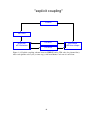
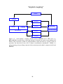
meshes, without any interpolation necessary. Also the “short-cycle” option, a semi-implicit
correction scheme for Monte Carlo source terms between large CFD ∆t cycles, without new
or at least with strongly reduced MC runs in between, was implemented.
Subsequently a large number of application runs, in particular those carried out at IPPGarching (Ralf Schneider et al.) and AEA-Culham Laboratories (Geoff Maddison) have
lead to identification of many critical issues and limitations of the code and to permanent
improvements until these days. Typical convergence behaviour of the combined code system (“saturated residuals”) is described in the new section 1.8, written in collaboration with
G.P.Maddison, AEA Culham Laboratories.
Detlev Reiter, Spring 1998
Foreword to 3rd edition
During the year 2001 a major revision of the EIRENE code has been carried out, largely in order to implement a somewhat more modern FORTRAN structure into the code. EIRENE code
versions from this particular year 2001 then have sometimes been referred to as “EIRENEFACELIFT” (= EIRENE2001 in the notation of this manual).
In particular a dynamical allocation of storage (rather than the hitherto necessary pre-assignment
of storage in the PARAMETER statements collected in the previous PARMUSR file) is now
in place. This dynamic memory management has led to a replacement of the previous
“Common-Blocks” now by “Modules”, and to the entire elimination of the “Equivalence”
statements used for storage economy in earlier versions.
Further main upgrades are related to:
• incident-species dependent surface interaction models, pumping speeds, sputter models etc., can now be controlled by input flags, rather than the previous quite difficult
implementation via the USR-routines.
• integration volumes of volume averaged tallies can now be larger than the grid cell
volumes, i.e., the plasma background and geometrical discretisation, which is not very
storage sensitive, can be made much finer than the neutral particle volume averaged
tally profile output.
2
• discretisation of general multiply connected 3D volumes by tetrahedron-grids.
• photons as new type of test particle species. The photon dummy module allows simple
photon transport (one-speed Boltzmann-equation) with spatial profiles of spontaneous
emission, Doppler line broadening, for optically thin lines only, with inclusion of (multiple) surface reflection. The full photon module additionally allows for various other
line broadening mechanisms and photon re-absorption, stimulated emission, radiation
trapping (excitation-hopping), iteration with neutral gas excitation population kinetics,
etc...
EIRENE versions 2003 and younger have been compiled and successfully tested at FZ-J¨ulich
on the following systems and compilers:
Linux: Suse 11.1 and all predecessors down to Suse 6.***:
• pgf90 Portland Compiler Version 5.2-4 — 10.1
• ifort Intel Fortran Compiler Version 8.1 — 11.1
• lf95 Lahey Fortran Compiler Version 6.2
• nagf95 NAG Fortran Compiler Version 5.0 — 5.2
AIX: AIX 4.3 und 5.2
• xlf95 XL Fortran for AIX Version 8.1
Windows: Windows 2000 und Windows XP
• Compaq Visual Fortran Version 6.6
Detlev Reiter, Spring 2010
3
Contents
1
The neutral gas transport equation;
Monte-Carlo terminology
1.1 The linear Boltzmann equation for the distribution function f . . . . . . . .
1.1.1 The WCU generalisation of the Boltzmann equation . . . . . . . .
1.2 The linear integral equation for the collision density Ψ . . . . . . . . . . .
1.2.1 The Green’s function concept . . . . . . . . . . . . . . . . . . . .
1.3 Monte Carlo solution of equation 1 . . . . . . . . . . . . . . . . . . . . . .
1.3.1 Unbiased estimators . . . . . . . . . . . . . . . . . . . . . . . . .
1.3.2 Scaling of tallies . . . . . . . . . . . . . . . . . . . . . . . . . . .
1.3.2.1 Scaling in problems with ignorable coordinates . . . . .
1.3.3 Statistical errors, Efficiency (FOM) . . . . . . . . . . . . . . . . .
1.3.3.1 Sampling, Non-analog sampling . . . . . . . . . . . . .
1.3.3.2 Stratified Source Sampling . . . . . . . . . . . . . . . .
1.3.4 Source sampling . . . . . . . . . . . . . . . . . . . . . . . . . . .
1.3.4.1 time-census sources . . . . . . . . . . . . . . . . . . . .
1.3.4.2 Point sources . . . . . . . . . . . . . . . . . . . . . . . .
1.3.4.3 Line sources . . . . . . . . . . . . . . . . . . . . . . . .
1.3.4.4 Surface-sources . . . . . . . . . . . . . . . . . . . . . .
1.3.4.5 Volume sources . . . . . . . . . . . . . . . . . . . . . .
1.3.5 Sampling a free flight from the transport kernel T . . . . . . . . . .
1.3.5.1 Alternative: fixed time step (or constant path length increment) . . . . . . . . . . . . . . . . . . . . . . . . . . . .
1.3.6 Sampling from the collision kernel C . . . . . . . . . . . . . . . .
1.3.7 elastic collisions . . . . . . . . . . . . . . . . . . . . . . . . . . .
1.3.8 charge exchange . . . . . . . . . . . . . . . . . . . . . . . . . . .
1.3.9 electron-impact collisions . . . . . . . . . . . . . . . . . . . . . .
1.3.10 general heavy-particle-impact collisions . . . . . . . . . . . . . . .
1.3.11 photon processes (emission, absorption, scattering) . . . . . . . . .
1.4 Surface Reflection Models . . . . . . . . . . . . . . . . . . . . . . . . . .
1.4.1 The Behrisch matrix reflection model . . . . . . . . . . . . . . . .
1.4.2 TRIM code database reflection models . . . . . . . . . . . . . . . .
1.5 Recycling surface sources . . . . . . . . . . . . . . . . . . . . . . . . . . .
1.5.1 half-sided Maxwellian flux at electrostatic sheath entrance . . . . .
1.5.2 The electrostatic sheath . . . . . . . . . . . . . . . . . . . . . . . .
1.5.3 The magnetic pre-sheath . . . . . . . . . . . . . . . . . . . . . . .
1.6 Combinatorial description of geometry . . . . . . . . . . . . . . . . . . . .
1.7 time dependent mode of operation . . . . . . . . . . . . . . . . . . . . . .
4
.
.
.
.
.
.
.
.
.
.
.
.
.
.
.
.
.
.
9
10
14
14
18
19
19
20
21
21
23
25
28
28
28
28
28
28
28
.
.
.
.
.
.
.
.
.
.
.
.
.
.
.
.
30
31
32
32
32
32
32
33
33
34
37
38
41
43
44
47
1.8
1.9
non-linear effects: coupling to plasma fluid models . .
non-linear effects: neutral-neutral collisions . . . . . .
1.9.1 BGK approximation . . . . . . . . . . . . . .
1.9.2 Direct Simulation (DMCS) of self-collisions .
1.10 Radiation transport, photon gas simulations . . . . . .
1.10.1 Line shape options . . . . . . . . . . . . . . .
1.11 Charged Particle Transport . . . . . . . . . . . . . . .
1.11.1 Orbit integration . . . . . . . . . . . . . . . .
1.11.1.1 Particles following the B-field . . . .
1.11.1.2 Guiding centre approximation . . . .
1.11.2 Coulomb Collision Models . . . . . . . . . . .
1.11.2.1 Simple Coulomb Collision Models .
1.11.2.2 The Fokker-Planck Collision Model
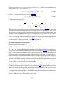
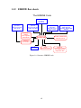
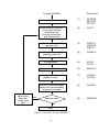
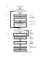
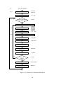
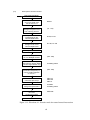
1.12 EIRENE flow charts . . . . . . . . . . . . . . . . . . .
2
.
.
.
.
.
.
.
.
.
.
.
.
.
.
.
.
.
.
.
.
.
.
.
.
.
.
.
.
.
.
.
.
.
.
.
.
.
.
.
.
.
.
.
.
.
.
.
.
.
.
.
.
.
.
.
.
.
.
.
.
.
.
.
.
.
.
.
.
.
.
48
54
55
56
56
57
59
59
59
60
60
60
62
63
Description of formatted input file
2.1 Input data for operating mode . . . . . . . . . . . . . . . . . . . . . .
2.1.1 Automated stratification optimization: proportional allocation
2.1.2 The NLERG option for cell volumes . . . . . . . . . . . . . .
2.1.3 The NLMOVIE option for making movies of trajectories . . .
2.2 Input for Standard Mesh . . . . . . . . . . . . . . . . . . . . . . . .
2.2.1 Mesh Parameters . . . . . . . . . . . . . . . . . . . . . . . .
2.3 The Input Block for Surfaces . . . . . . . . . . . . . . . . . . . . . .
2.3.1 The Input Block for “Non-default Standard Surfaces” . . . . .
2.3.2 Input Data for “Additional Surfaces” . . . . . . . . . . . . . .
2.4 Input Data for Species Specification and Atomic Physics Module . . .
2.4.1 Default atomic and molecular data . . . . . . . . . . . . . . .
2.4.2 Neutral-Neutral collisions in BGK approximation . . . . . . .
2.4.3 Fitting expressions (IFTFLG) . . . . . . . . . . . . . . . . .
2.5 Input for Plasma Background . . . . . . . . . . . . . . . . . . . . . .
2.5.1 Derived Background Data . . . . . . . . . . . . . . . . . . .
2.6 Input Data for Surface Interaction Models . . . . . . . . . . . . . . .
2.6.1 effective pumping speed . . . . . . . . . . . . . . . . . . . .
2.7 Input data for Initial Distribution of Test Particles . . . . . . . . . . .
2.7.1 Piecewise constant “Step-functions” for sampling . . . . . . .
2.7.2 Electrostatic sheath acceleration . . . . . . . . . . . . . . . .
2.8 Additional Data for some Specific Zones . . . . . . . . . . . . . . . .
2.9 Data for Statistics and non-analog Methods . . . . . . . . . . . . . .
2.10 Data for additional volume and surface averaged tallies . . . . . . . .
2.10.1 Additional volume averaged tallies, tracklength estimator . . .
2.10.2 Additional volume averaged tallies, collision estimator . . . .
2.10.3 Algebraic expression in volume averaged tallies . . . . . . . .
2.10.4 Algebraic expression in surface averaged tallies . . . . . . . .
2.10.5 Algebraic expression in surface averaged tallies . . . . . . . .
2.10.6 Energy spectra in selected cells or surfaces . . . . . . . . . .
2.11 Data for numerical and graphical Output . . . . . . . . . . . . . . . .
2.12 Data for Diagnostic Module . . . . . . . . . . . . . . . . . . . . . .
.
.
.
.
.
.
.
.
.
.
.
.
.
.
.
.
.
.
.
.
.
.
.
.
.
.
.
.
.
.
.
.
.
.
.
.
.
.
.
.
.
.
.
.
.
.
.
.
.
.
.
.
.
.
.
.
.
.
.
.
.
.
.
.
.
.
.
.
.
.
.
.
.
.
.
.
.
.
.
.
.
.
.
.
.
.
.
.
.
.
.
.
.
.
.
.
.
.
.
.
.
.
.
.
.
.
.
.
.
.
.
.
.
.
.
.
.
.
.
.
.
.
.
.
69
73
79
79
80
81
91
92
92
95
106
123
126
127
129
136
137
149
150
164
166
167
169
173
174
175
176
176
176
177
179
190
5
.
.
.
.
.
.
.
.
.
.
.
.
.
.
.
.
.
.
.
.
.
.
.
.
.
.
.
.
.
.
.
.
.
.
.
.
.
.
.
.
.
.
.
.
.
.
.
.
.
.
.
.
.
.
.
.
.
.
.
.
.
.
.
.
.
.
.
.
.
.
.
.
.
.
.
.
.
.
.
.
.
.
.
.
.
.
.
.
.
.
.
.
.
.
.
.
.
.
2.12.1 Line of sight: charge exchange spectrum . . . .
2.12.2 Line of sight: line emissivity . . . . . . . . . . .
2.12.3 Line of sight: line shape . . . . . . . . . . . . .
2.12.4 Line of sight: user defined integral . . . . . . . .
2.13 Data for nonlinear and time dependent Options . . . . .
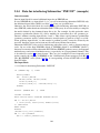
2.14 Data for interfacing Subroutine “INFCOP” (example) . .
2.14.1 Version B2-EIRENE-1999 and older . . . . . . .
2.14.2 Version B2-EIRENE-2000 and younger . . . . .
2.14.3 Version B2-EIRENE-wide-grid (2011 and later) .
2.14.4 Version B2.5-EIRENE (2012 and later) . . . . .
.
.
.
.
.
.
.
.
.
.
194
194
194
194
195
198
199
206
209
209
3
Problem specific Routines
3.1 Parameter Statements (for EIRENE-2001 or older) . . . . . . . . . . . . . .
3.2 The “Additional Tally” routines UPTUSR, UPCUSR, UPSUSR and UPNUSR
3.2.1 Tracklength estimated volume tallies, UPTUSR . . . . . . . . . . . .
3.2.2 Collision estimated volume tallies, UPCUSR . . . . . . . . . . . . .
3.2.3 Snapshot estimated volume averaged tallies, UPNUSR . . . . . . . .
3.2.3.1 A: time dependent estimates . . . . . . . . . . . . . . . . .
3.2.3.2 B: stationary snapshot tallies . . . . . . . . . . . . . . . .
3.2.4 Surface averaged tallies, UPSUSR . . . . . . . . . . . . . . . . . . .
3.3 The user surface reflection model REFUSR . . . . . . . . . . . . . . . . . .
3.4 The user source sampling routine SAMUSR . . . . . . . . . . . . . . . . . .
3.5 The user routines to overrule input data . . . . . . . . . . . . . . . . . . . .
3.5.1 The user geometry data routine GEOUSR . . . . . . . . . . . . . . .
3.5.2 User supplied background data routine PLAUSR . . . . . . . . . . .
3.6 The user routines for profiles PROUSR . . . . . . . . . . . . . . . . . . . .
3.7 User supplied post-processed tally routine TALUSR . . . . . . . . . . . . . .
3.8 User supplied “general geometry block” . . . . . . . . . . . . . . . . . . . .
3.8.1 Subroutine INIUSR . . . . . . . . . . . . . . . . . . . . . . . . . . .
3.8.2 Subroutine LEAUSR . . . . . . . . . . . . . . . . . . . . . . . . . .
3.8.3 Subroutine TIMUSR . . . . . . . . . . . . . . . . . . . . . . . . . .
3.8.4 Subroutine VOLUSR . . . . . . . . . . . . . . . . . . . . . . . . . .
3.8.5 Subroutine NORUSR . . . . . . . . . . . . . . . . . . . . . . . . . .
211
213
217
218
218
219
219
220
220
222
224
226
226
227
227
229
229
229
230
230
231
231
4
Routines for interfacing with other codes:
EIRCOP
4.1 Routine for interfacing INFCOP . . . . . . . . . . . . . . . . . . . . . . .
4.1.1 entry IF0COP . . . . . . . . . . . . . . . . . . . . . . . . . . . . .
4.1.2 entry IF1COP . . . . . . . . . . . . . . . . . . . . . . . . . . . . .
4.1.3 entry IF2COP(ISTRA) . . . . . . . . . . . . . . . . . . . . . . . .
4.1.4 entry IF3COP(ISTRAA,ISTRAE) . . . . . . . . . . . . . . . . . .
4.1.5 entry IF4COP . . . . . . . . . . . . . . . . . . . . . . . . . . . . .
4.2 Routines for cycling of EIRENE with external codes: EIRSRT . . . . . . .
4.3 Routines for special tallies needed for code coupling: UPTCOP . . . . . . .
4.4 Statistical noise in Monte Carlo terms for external code, noise-residuals:
STATIS COP . . . . . . . . . . . . . . . . . . . . . . . . . . . . . . . . .
6
.
.
.
.
.
.
.
.
.
.
.
.
.
.
.
.
.
.
.
.
.
.
.
.
.
.
.
.
.
.
.
.
.
.
.
.
.
.
.
.
.
.
.
.
.
.
.
.
.
.
.
.
.
.
.
.
.
.
.
.
.
.
.
.
.
.
.
.
.
.
.
.
.
.
.
.
.
.
.
.
.
.
.
.
.
.
.
.
.
.
.
.
.
.
.
.
.
.
.
.
.
.
.
.
.
.
.
.
232
232
233
234
234
234
235
235
235
. 236
5
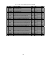
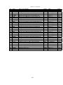
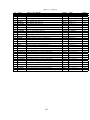
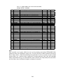
Default EIRENE tallies, and selected Modules
5.1 Tables of EIRENE tallies . . . . . . . . . . . . . . . . . . . . . . . . . . . .
5.1.1 Current status, incl. photon gas tallies (Eirene2002 and younger) . . .
5.1.2 old version, w/o photon gas tallies (Eirene2001 and older) . . . . . . .
References
7
237
237
239
247
Introduction and General Information
This manual describes the input required by the EIRENE code to run a Monte Carlo study
for a fully 3 dimensional simulation of linear transport (i.e., of test particles) in a prescribed
background medium. Although the geometry of the problem and the interaction between test
particle species and the background are in principle not subject to any restrictions, the aim
of code development was to provide a tool for investigating neutral gas transport in tokamak
plasmas. Consequently the choice of preprogrammed options has been made mainly with
this application in mind. A large variety of problems in this field can be run without having
to resort to any problem specific routines but instead by an appropriate setting of logical and
numerical input flags.
Any user of EIRENE should be aware that this code is a moving target as is this manual.
Therefore it is possible that there are some inconsistencies between this description and a
particular version of the code. The user should always first check subroutine INPUT, where
most of the data are read in using hard wired formats, as most input errors will lead to a rapid
exit in the initialization phase of a run.
This manual was written by the author of the code who often may not have been able to
anticipate difficulties in understanding the use of EIRENE. He therefore gratefully acknowledges any suggestions to make this manual more informative and clear than it might be at the
present status.
This code description consists of the following parts:
• In the first part an introduction is given to the general linear transport problem and its
solution by Monte Carlo methods. Most of the terminology used in later sections is
introduced there.
• In part two a description of the formatted input file required by EIRENE to run on a
specific problem is given. It mainly consists of explanations of the meanings of the
various input flags.
• In part three the most important problem specific routines are explained. At present we
have restricted this part to routines for evaluation of “user requested tallies”, namely
the subroutines UPTUSR, UPCUSR and UPSUSR. Other often applied routines such
as SAMUSR (user supplied source sampling distribution) or REFUSR (user supplied
surface interaction model) are briefly described.
• In part four the package EIRCOP for interfacing EIRENE with other codes (e.g., the
B2-EIRENE package) is described. Here mainly the location of the storage on the
EIRENE work array RWK for plasma data and geometrical information is given. Also
the implementation of the method of (semi-implicit) corrections (see section 1.8) at
each plasma code time-step to the terms transferred from EIRENE to plasma fluid
transport codes is described here.
8
Chapter 1
The neutral gas transport equation;
Monte-Carlo terminology
General Remarks
To introduce the terminology used throughout this report, we briefly recall the basic definitions and principles of a Monte Carlo linear transport model, following the lead of many
textbooks on Monte Carlo methods for computing neutron transport (see e.g., [8]). We begin
with the linear transport equation for the pre-collision density, written as integral equation
(linear non-homogeneous Fredholm integral equation of 2nd kind). Distinct from standard
terminology in the (analytic) transport theory we do not discuss analytic properties of the various terms in the equation, but, instead, point out their probabilistic interpretation, as needed
for a Monte-Carlo solution of that equation. Next (section 1.3) we sketch the Monte Carlo
procedure to solve such equations, by referring to the two most often applied techniques:
”track-length - and collision based estimators”. In the third subsection we briefly describe
the treatment of boundary conditions (models for interaction of the particles with surrounding surfaces) and discuss some special models which are in use for the neutral gas transport
in fusion plasma devices. Then (section 1.5) we discuss the most important source function
(non-homogeneous part of the integral equation) and its implementation in a Monte Carlo
algorithm, namely the surface source of neutral particles due to recombination of ions incident on solid surfaces at the boundary or inside of the computational area. In section 1.6 we
comment on the implementation of geometry within the framework of a Monte Carlo code
in general terms and for the EIRENE code in particular. In section 1.7 the time dependent
mode of operation of the EIRENE code is described. It merely amounts just to an increase in
the dimensionality by one, by adding a time co-ordinate and treating it, formally, in a rather
symmetric fashion with the other spatial coordinates. See also reference [9].
Two kinds of non-linearities may be accounted for:
In section 1.8 the nonlinear behavior resulting from background data, which depend on neutral particle transport (sources and sinks), is discussed. The algorithm of the B2-EIRENE
code system [3] is described. More details on this can be found in the report [10].
In the final section of this introductory chapter 1.9 the non-linear BGK formalism and the direct simulation method (DMCS) for self collisions between neutral particles, as implemented
in the EIRENE code, is described.
9
1.1
The linear Boltzmann equation for the distribution function f
EIRENE solves a multi species set of coupled “Boltzmann”-type equations, in arbitrary 3D
geometries. Strictly speaking it is the Boltzmann equation generalized from its original single
species form with bi-linear collision kernel for elastic collisions, to a far more complicated
collision integral, which also represents “chemical reactions”. This generalisation is also
often referred to as Wang Chang-Uhlenbeck (WCU) equation in literature [11]. In this present
section we start with the Boltzmann equation. We then deal with linearisations of collision
kernels by fixing the phase space distribution of one of the two collision partners (which we
refer to as “bulk” or “background” or even simply “plasma” species). Generalization to the
full WCU type multi-species collision kernels, which in the same linearised form provide the
mathematical description of the equations solved by EIRENE, is then discussed next, section
1.1.1. Relaxation of the linearisation is needed only when there is self-interaction amongst
the species considered by EIRENE, as it is required e.g. when radiation transfer is included
(coupling between “photons” and atoms) or if neutral-neutral collisions are relevant. In this
latter case so called BGK approximations to the full collisions integral are employed, and the
non-linearity is dealt with by successive linearisation (i.e. by iteration).
The strongest non-linearity in EIRENE applications is typically the back-reaction of the
“plasma-background” (the host medium) on the neutral gas and radiation fields. This, however, is dealt with in an operator splitting cycling procedure (see section 4) between a plasma
solver (“diffusion-advection sub-module” solver, for given reaction term) and EIRENE (“reaction part” solver, for given diffusion advection solution, i.e. for given background medium),
in which EIRENE, within each single cycle, may still be operated in linear mode.
The term µ-space in this report refers to the phase space of a single particle. The quantity of
interest is then the one particle distribution function f
f (r, v, i, t)
or f˜(r, E, Ω, i, t)
or f (x),
where the state x of the µ-space is characterized by a position vector r, a velocity vector v, a
species index i (i stands for, e.g., H, D, T, D2 , DT, He, CHn ,...) and the time t.
The number density ni (r) for species i then reads:
∫
ni (r, t) = d3 v f (r, v, i, t)
Instead of v we sometimes utilize the kinetic energy E, E = m/2 · v 2 , and the unit (speed)
vector Ω = v/|v| in the direction of particle motion. Hence:
f (r)d3 v = f˜(E, Ω)dEdΩ
where d3 v = v 2 dvdΩ
and
f (r, v, i, t) =
(m)
v
and dΩ = sin θdθdϕ
f˜(r, E, Ω, i, t)
The distribution function in the form of f˜ clearly remains meaningful also in the case of
massless particles (photons), i.e. for applications of EIRENE to radiation transfer problems.
10
We start with the (elastics only) “Boltzmann Equation” [12], but by assuming additionally
that collisions are discontinuous events (i.e.: finite range interaction potentials, or, at least,
that proper cut-off procedures are applicable). This additional assumption allows us to separate, in the Boltzmann collision integral, the collisional loss and gain terms
∫∫∫into two′ separate
integrals. Otherwise cases could arise in which only the net collision term
. . . (f fb′ −f fb )
would lead to finite
∫∫∫
∫∫∫results, but not the collision term in the form as given in (1.1a) below:
′ ′
. . . (f fb ) −
. . . (f fb ).
Further: Lets consider only one specific species i0 , now omitting this species index. We assume that there are only collisions of this species i0 with only one further species, here labeled
b, anticipating that later, when discussing linear models, these species will be referred to as
background species, plasma species, etc.., with an externally given distribution fb (x, v, t).
Restriction here to elastic collisions means that exactly one particle of each of these two
species will also be present after the collision event (i.e., chemical reactions, inelastic collisions with change of internal energy, are excluded for the time being, but their description is
discussed below, section 1.1.1). The familiar Boltzmann equation for the distribution function
f for this species i0 reads
∂
F(r, v, t)
[ + v · ∇r +
· ∇v ] f (r, v, t) =
∂t
m
−
∫ ∫ ∫
∫ ∫ ∫
σ(v′ , V′ ; v, V)|v′ − V′ |f (v′ )fb (V′ )
σ(v, V; v′ , V′ )|v − V|f (v)fb (V)
+ Q(r, v, t)
(1.1a)
There is one such equation for each “particle species i” considered, but for elastic collision
without exchange between species always only two of them (here: i0 and b) a directly coupled
to each other.
Q(= Qi0 ) is any external source (particles per unit time injected per unit volume in phase
space).
Integrations are over the pre-collision velocities v′ , V′ as well as over one of the two post
collision velocities: V. σ(v′ , V′ ; v, V) is the differential cross section for a binary particle
collision process. The product of this σ with the relative pre-collision velocity is the transitional probability. The four velocity arguments are not truly independent: the conservation
laws for total energy and momentum must be fulfilled.
mi0 v′ + mb V′ = mi0 v + mb V
1
1
1
mi0 v ′2 + mb V ′2 =
mi v 2 + mb V 2 + ∆ E
2
2
2 0
(1.2)
Here ∆E is the exchange of internal energy in the collision (on expense of the energy of
relative motion), ∆E = 0 for elastic collisions. We may assume that σ contains appropriate
delta function factors such that integrations over velocity space reduce to integrations over
the lower dimensional manifolds on which these conservation laws are fulfilled.
The first two arguments in σ, namely the velocities v′ , V′ in the first integral, correspond to
the species i0 and b, respectively, prior to a collision. These are turned into the post collision
velocities v, V, again for species i0 and b, respectively. The first integral, therefore, describes
transitions (v′ , V′ → v, V) into the velocity space interval [v, v + dv] for species i0 , and the
second integral describes loss from that interval for this species.
11
Furthermore, m = mi0 is the particle mass and F(r, v, t) is the volume force field.
The right hand side is the collision integral δf
| . If there are more than just one possible
δt coll
type of collision partners (species) “b”, then the collision integral has to be replaced by a sum
of collision integrals over all collision partners b, including, possibly, b = i0 (self collisions)
∑ δf
δf
δf
δf
|coll =
|gain − |loss =
| .
(1.3)
δt
δt
δt
δt collb
b
All these collision operators are bi-linear in the distribution functions fi0 , fb . The first term
on the right hand side is due to scattering into the element dv of velocity space and we shall
abbreviate it by defining the collision kernel (“redistribution function”) C as a proper integral
over pre- and post collision velocities of species b-particles:
∫
δf
|
= d3 v ′ C(v′ → v)|v′ |f (v′ )
(1.4)
δt gain
In addition to being an integral over particle “b” velocity distributions, the kernel C can
be a quite complicated integral due to collision kinetics, as is involves not only multiple
differential cross sections, but also, possibly, particle multiplication factors, e.g. in case of
fission by neutron impact, dissociation of molecules by electron impact, or stimulated photon
emission from excited atoms. It can also include absorption, in which case the post collision
state must be an extra “limbo” state outside the phase-space considered. Due to both particle
multiplication and/or absorption the collision kernel C is not normalized to one, generally.
If the distributions fb of one of the collision partners are assumed to be given (see below:
linear Boltzmann equation), then the kernel C is linear and the expression above becomes a
linear integral operator.
The second term on the right hand side is much simpler, because the function f (v) can be
taken out of the integral. We even take the product |v| · f before the integral. The remaining
integral is then just the total macroscopic cross section Σt , i.e., the inverse local mean free
path (dimension: 1/length). It is solely defined by total cross sections and independent of
particle multiplication factors, since we only consider binary collisions (exactly two precollision partners always).
This term is then, often, taken on the left hand side of the Boltzmann equation with a positive
sign, in the form:
δf
| = Σt (r, v)|v|f (v)
(1.5)
δt loss
linear form of Boltzmann transport equation
For the linear case (fb given for all collision partners other than i0 and self collisions being
excluded, then this “extinction coefficient” Σt is independent of the dependent variable f =
fi0 , and this term (out-scattering) just describes the loss of particle flux of i0 particles due to
any kind of interaction of them with the host medium.
With these formal substitutions the Boltzmann equation takes a form which is often more
convenient, in particular in linear transport theory:
∫
∂
F(r, v, t)
[ + v · ∇r +
· ∇v ] f (r, v, t) + Σt (r, v)|v|f (v) =
d3 v ′ C(v′ → v)|v′ |f (v′ )
∂t
m
+ Q(r, v, t)
(1.1b)
12
which, in the linear case (no self collisions, fb given externally) is a linear equation for the
distribution function f = fi0 (x, v, t) for species i0 .
Clearly a computationally crucial simplification is provided in this linear case, which means
neglect of all interactions within the community of species “i”, retaining only: i0 + b → · · ·
events. In practice for neutral particle transport in plasmas this mostly means neglect of
neutral-neutral interaction, retaining only neutral-plasma collisions (for given plasma conditions). For the status of options in EIRENE to deal with “non-linear” “self-collisions”
(i0 + i0 → · · · ) or with “cross collisions” (i0 + i1 → · · · ) amongst the species for which the
kinetic equation is solved, see below, section 1.9.
stationary kinetic transport equation
Often the characteristic time constants for neutral particle transport phenomena are very short
(µs), compared to those for plasma transport (ms). We can, therefore, often neglect explicit
time dependence in the equations describing the neutral particles. This is done in most applications. The extension to time-dependent problems is rather straight forward and the procedure in the EIRENE code for such cases is described in 1.7 below.
For stationary (time-independent) problems the scalar transport flux (“angular flux”) Φ, where
Φ(x) := |v| · f (r, v, i),
(1.6a)
is sometimes used as dependent variable, in preference to the distribution f (x).
In particular for stationary (∂/∂t = 0) and force free (F = 0) problems, as e.g. often
encountered in linear transport theory such as neutronics, radiation transport, neutral particle
transport in plasmas, etc., the transport equation then reduces to the more compact form:
∫
∇r Φ(r, v, t) + Σt (r, v)Φ(r, v) = Q(r, v, t) + d3 v ′ C(r; v′ → v)Φ(r, v′ )
(1.1c)
Alternatively, in computational domains with non-vanishing collisionality (i.e., if Σt (x) ̸= 0
everywhere) the (pre-) collision density Ψ is used, i.e.,
Ψ(x) = Σt (x) · Φ(x) = νt (x) · f (x),
Σt = Σt (r, E, Ω, i) = νt (r, E, Ω, i)/|v| (1.2)
where, again, the “macroscopic cross section” Σt is the total inverse local mean free path (dimension: 1/length), and νt is the
∑collision frequency (dimension: 1/time). This cross section
can be written as a sum Σt =
Σk over macroscopic cross sections for the different types
(identified by the index k) of collision processes. Further details about this “macroscopic
cross section” and its relation to the conventional (“microscopic”) cross sections are given
below, section 1.3.5.
In closing this section we note:
All these equations 1.1a, 1.1b, 1.1c, and equation 1.1d given below are equivalent, of course,
as well as their WCU generalizations discussed in the next section 1.1.1. Which particular
form is used in a particular discussion depends upon the issue which is considered. For
example, the collision estimator for evaluating moments (responses) of the solution to the
Boltzmann equation can be shown to be unbiased quite conveniently when using eq. 1.1d,
whereas the tracklength estimator, used for the same purpose in EIRENE, is most easily
understood with the from 1.1d. Time dependent cases are best discussed utilizing the form
1.1b, etc...
13
1.1.1
The WCU generalisation of the Boltzmann equation
The mathematical generalization from the classical Boltzmann equation (for a system undergoing only elastic collisions) to the semi-classical Boltzmann equation (the WCU equation,
[11]) for chemical reactions (including, for example, vibrational relaxation or exchange of
internal energy as special cases) symbolized as li′ , lb′ li , lb is outlined here. These species
indices label both the chemical species and/or the internal quantum state. I.e. we regard
two particles (objects) as different, with a different label, if either they belong to a different
chemical species or they differ by their internal (electronic, or ro-vibrational, etc) state, as
appropriate).
As above, linearisation will be obtained by grouping labels li and lb into two disjunct classes,
and allowing for reactions only between initially (prior to the collision) one member from
class “i” and one member from class “b”. If we consider then the phase-space balance equation for a given species li0 then the sum in the collision integral is over velocities belonging
to all pre-collision labels li′ , lb′ and over velocities of “species” lb (more generally: over all
velocities except those from the one post collision label li0 , in case of more than two post
collision particles).
l ,l
The cross sections in the corresponding collision integrals σl′i0,l′ b (v′ , V′ , v, V) are multiple
i b
differential for scattering at a certain solid angle and post collision energies with simultaneous transition from (li′ , lb′ ) to (li , lb ). For more than two post collision objects (e.g. fission,
dissociative excitation, stimulated radiation emission, etc...), this notation is readily generalized by adding more superscript labels and more post collision velocities. Thus the full WCU
prototypical system of kinetic transport equations then reads (for two post collision particles)
to be written, f or ref erence purpose only .....not needed explicitly here
(1.7)
The extra discrete label l introduced here compared to the Boltzmann equation may either
be regarded as species index: i0 → i0 , l or as other additional discrete independent variable
(e.g. polarization, in case of radiation transport): fi0 (v) → fi0 (l, v), whichever is more
convenient.
As noted above, further generalizations to include particle splitting, absorption or fragmentation into more than two post collision products are straight forward, but can more conveniently be formulated in the C-collision kernel formulation introduced above and used below
to relate the transport equation to a Markovian stochastic (discrete time) process.
1.2
The linear integral equation for the collision density Ψ
By formally integrating the characteristics for (1.1c) the same transport equation can also be
written in integral form. This formal procedure is outlined below in paragraph 1.2.1.
The resulting integral equation is often most conveniently written for the collision density Ψ
(1.2) rather than for transport flux Φ:
∫
Ψ(x) = S(x) + dx′ Ψ(x′ ) · K(x′ → x).
(1.1d)
This equation has the general form of the backward integral equation of a Markovian jumpprocess and it is therefore particularly well suited for a Monte Carlo method of solution.
The formal relation between the integro-differential form (1.1c) and this integral form is very
14
useful to generalize the Monte Carlo procedure, e.g., to time-dependent equations, and to
Boltzmann-Fokker-Planck equations (which contain diffusive contributions or diffusive approximations for some processes, in addition to the jump processes described by the Boltzmann collision integral). It also allows to make connection to the so called “Green’s-functions
Monte Carlo” concept (originally developed for quantum mechanical problems involving solutions to the Schr¨odinger equation). A corresponding discussion is postponed to section
1.2.1. A direct intuitive interpretation of the integral equation is already sufficient to understand the Monte Carlo method of solution and shall be given first.
∫
In (1.1d) x′ and x are the states at two successive collisions (jumps). The integral dx′ in
(1.1d) is to be understood as an integral over all initial coordinates, i.e. over the entire physical
space, the full velocity space and a summation over all species indices. The transition kernel
K is usually decomposed, in our context, into a collision- and a transport kernel, i.e., C and
T , where
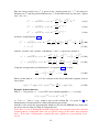
K(r′ , v′ , i′ → r, v, i) = C(r′ ; v′ , i′ → v, i) · T (v, i; r′ → r).
(2.8)
The kernel C is (excluding normalization) the conditional distribution for new co-ordinates
(v,i) given that a particle of species i′ and with velocity v′ has undergone a collision at
position r′ . This kernel can further be decomposed into:
C(r′ , v′ , i′ → v, i) =
∑
pk Ck (r′ ; v′ , i′ → v, i) , pk =
k
Σk
Σt
(2.9)
with summation over the index k for the different types of collision processes under consideration and pk defined as the (conditional) probability for a collision to be of type k. The
normalizing factor
∑∫
1
′
d3 v Ck (r′ , v′ , i′ → v, i) , Ck = Ck
ck (x ) =
(2.10)
ck
i
gives the mean number of secondaries for this collision process. The function Ck then is a conditional probability density. The particle absorption process can conveniently be described
by adding an “absorbing state” xa to the µ-space (generally referred to as “one-point compactification of this space” in the language of mathematical topology). This “limbo state”,
once it is reached, is never left again if the kernels T or C are employed as transition probabilities. Formally, an additional collision kernel Ca (x → xa ) and an absorption probability
pa = Σa /Σt must be included in the collision kernel. The quantity Σa comprises all collision
processes with no next generation particles within the community of particles considered by
the coupled set of kinetic transport equations. (Ionisation of a neutral atom is a loss, if the
resulting ion is not considered further, or dealt with by a CFD code outside the Monte Carlo
procedure).
The kernel T describes the motion of the test particles between the collision events. Let,
again, Ω′ denote the unit vector in the direction of particle flight v′ /|v′ |, and let Ω′2 and Ω′3
be two further unit vectors such that these three vectors form an orthonormal basis at the point
r′ . Neither velocity nor species change along the transition described by T , i.e. v′ = v and
i′ − i. Omitting the corresponding delta functions in velocity space and the Kronecker delta
15
δi′ i the transport kernel T then reads as follows:
[ ∫
(T (l) =) T (v′ , i′ ; r′ → r) = Σt (r, v′ , i′ ) · exp −
l=Ω′ (r−r′ )
]
dsΣt (r′ + sΩ′ , v′ , i′ )
0
=
·δ(Ω′2 (r − r′ )) · δ(Ω′3 (r − r′ ))
Σt (r, v′ , i′ ) · F (v′ , i′ ; r′ → r)
· H(Ω′ (r − r′ ))
0≤l≤∞
(2.11a)
(2.11b)
with H(x) = 0 if x < 0, and H(x) = 1 if x ≥ 0, the Heaviside step function (the unit step
function). The two remaining delta functions restrict the motion to a path in the direction of
the initial velocity v′ .
Thus, although strictly being a conditional (on x′ ) distribution in phase space, for an infinite
medium T can be interpreted as the distribution density for the distance l for a free flight
starting from r′ to the next point of collision r = r′ + l · Ω′ . We shall frequently omit
the arguments v′ , i′ to simplify notation, because neither initial velocity nor species change
during a free flight.
For a finite medium this distribution can be generalized to (writing shorter l for (r′ +lΩ′ , v′ , i′ ):

[ ∫
]
l
 Σt (l)
· exp − 0 dsΣt (s) , l < lmax
[ ∫
]
T (l) =
(2.12)
 δ(l − lmax ) · exp − lmax dsΣt (s) , l ≥ lmax
0
Here lmax denotes the distance along the flight direction from r′ to the boundary for the
computational domain, to any internal surface at which the test flight shall be stopped, e.g.
for scoring surface fluxes there, or even to the cell boundary. The “Transport Kernel” T has
dimension: [1/Dimension of phase space] (T (x′ → x)dx is a probability). The function F
(Dimension: [length times Dimension of T ]) defined in expression (2.11b), and analogously
from (2.12) for a finite medium, will turn out to be the relevant Green’s function for the
transport problem, see Section 1.2.1. The integral
∫ Ω(r−r′ )
′
α(r , r) =
dsΣt (r′ + sΩ)
0
in equation (2.11a) is well known as “optical thickness of the medium” in linear transport
theory.
The inhomogeneity S in equation (1.1d) is, excluding normalization, the distribution density
of first collisions, whereas the integral term in equation (1.1d) describes the contribution to
Ψ from all higher generations. The quantity S can be written as:
∫
S(x) = dx′ Q(x′ ) · T (x′ → x),
(1.6a)
with a source density Q. As the problem is linear, Q can be normalized to 1 and, thus, Q
can be considered a distribution density in µ -space for the “primary” birth points of particles,
as, e.g., opposed to the “secondary” birth point distribution (or “post collision density”) χ of
particles after a collision event
∫
χ(x) = dx′ Ψ(x′ ) · C(x′ → x).
(1.6b)
16
It can be shown that a unique solution Ψ(x) exists subject to appropriate boundary conditions
and under only mild restrictions (basically on the constants ck and pa ) to ensure that the
particle generation process stays sub-critical.
Usually, a detailed knowledge of Φ or Ψ is not required, but only a set of “responses”, R,
defined by
(
)
∫
∫
R = < Ψ|gc > = dxΨ(x) · gc (x)
= < Φ|gt > = dxΦ(x) · gt (x) , (2.13)
where gc (x), gt (x) are given “detector functions”.
For example all terms in the plasma fluid equations resulting from neutral plasma interaction
can be written in this way. This can be seen by considering a numerical grid, composed of
M mesh cells (spatial and/or temporal), for the numerical solution of the fluid equations. The
detector functions for many responses needed for fusion plasma applications are hard wired
in EIRENE, generalization to any arbitrary response by resorting to “user defined detector
functions” is described in Section 3.2.1 for tracklength estimates, and in Section 3.2.2 for
collision estimates.
Lets therefore define an entire set of detector functions gm , one for each mesh cell of an
external code, each including a characteristic function
gm = g × chm (r, t),
m = 1, 2, ..., M,
(2.14a)
i.e., chm (r, t) = 1 inside the numerical mesh cell (or time interval) labeled with the cell index
m, and chm (r, t) = 0 outside this cell. Thus profiles of cell volume averaged responses are
readily obtained in a single Monte Carlo run.
Estimates of surface fluxes, or point estimates e.g. in time, are also included in this concept
if proper use is made of delta functions to reduce dimensionality of the response:
gm,α = g × chm (r, t) × δ α (r, t),
m = 1, 2, ..., M,
(2.14b)
Here, e.g., a surface cell m would discretise a surface S characterized by a surface delta
function δ S .
Equation (2.13) shows that Monte Carlo estimates (tallies) fall into the category of extensive
quantities (number of particles, total energy, momentum, etc., per cell). Intensive quantities (flow velocity, temperature, etc...) obtained by dividing two extensive quantities are
typically difficult estimate with Monte Carlo methods (see: “ratio estimates”, correlation between nominator and denominator,...). If, however, the extensive quantity in the denominator
is known exactly, such as e.g. the cell volume in a computational mesh, then, of course,
obtaining an intensive quantity from an extensive quantity with Monte Carlo is a trivial rescaling.
Monte Carlo estimates of the (intensive) volumetric source terms in the fluid equations due
to the trace particles (neutral particles, but also trace ions described by the Monte Carlo
procedure) are such cell averages, surface averages, time averages or point estimates (e.g. in
time), averaged over a sub-manifold with reduced dimensionality. (This works, of course,
only if the probability for particle histories crossing this sub-manifold is not zero). Surface
averages in EIRENE are described in Section 3.2.4, point averages in time are described
in Section 3.2.3. This option to reduce dimensionality of responses usually excludes point
estimates in real space, for which special estimators not mentioned here would be required.
Nevertheless, in concluding, depending upon the numerical algorithm in the fluid code, one
may then have to interpret these Monte Carlo estimates properly, e.g. they may have to be
interpolated to the grid points, or be properly rescaled in case of time-dependent applications.
17
1.2.1
The Green’s function concept
We return to Equation (2.11b), where the function F (v, i; r′ → r)) was defined. For a finite
domain, see (2.12), and introducing again the shortcut l for (r′ + lΩ, v, i) this becomes:
[ ∫
]
{
l
exp − 0 dsΣt (s) , l < lmax
F (l) =
(2.15)
0
l ≥ lmax
This function F is the Green’s function of the left hand side (the “convective part”) of the
transport equation.
to be written
18
1.3
Monte Carlo solution of equation 1
A statistical solution to equation (1.1b) is straight forward, because it is formulated in probabilistic terms as follows.
A discrete Markoff chain is defined using Q as an initial distribution and L = T · C (order of
C and T reversed compared to K) as a transition probability. Histories ω n from this stochastic
process are generated according to ω n = (x0 , x1 , x2 , ..., xn ), (where xj = xa for all j ≥ n and
xi ̸= xa for all i < n), with xn being the first state after transition into the absorbing state xa .
x0 denotes the initial state distributed as described by Q. Thus, the length n of the chain ω n is
itself a random variable. A random sampling procedure to generate such chains is carried out
in Monte Carlo codes by converting machine generated (pseudo-) random numbers ξi1 , ξi2 , ...
into random numbers with the distributions Q, T and C. Having computed N chains ωi ,
i = 1, 2, ..., N , the responses R (2.13) with respect to detector function g are estimated as the
arithmetic mean of functions (“statistics”, or “estimators”) Xg (ω), i.e.
N
1 ∑
˜
Xg (ωi ).
R≈R=
N i=1
(3.16)
The proper choice of the number of histories N depends on the variance σ 2 (Xg ) of the estimator Xg and is highly problem specific. In EIRENE it can range from N = 2 for conditional
expectation estimators and point sources in phase space, up to values of several millions for
N.
1.3.1
Unbiased estimators
One possible choice for X(ω) is the so called “collision estimator” X c ,
Xgc (ωin ) =
n
∑
gc (xl ) ·
l=1
l−1
∏
c(xj )
.
(1
−
p
(x
))
a
j
j=1
(3.17)
This estimator is, for example, used in the DEGAS code [13]. It can be shown [8] in a tedious
but mathematically strict way that the statistical expectation E(X c ) produces:
∫
c
R = E(X ) = d(ω)Xgc (ω)h(ω)
(3.18)
with h(ω) being the probability density for finding a chain ω from the Markoff process defined above, i.e. X c is an unbiased estimator for R.
Other estimators (“track-length type estimators”) are employed frequently. These estimators
are unbiased as well but have higher moments different from those of X c . Instead of evaluating the detector function gc (x) at the points of collisions, xl , (as X c does,) they involve line
integrals of gt (x) along the trajectories, e.g.,
} ∏
l−1
n−1 {∫ xl+1
∑
c(xj )
t
n
ds gt (s) ·
Xg (ωi ) =
,
(3.19)
(1 − pa (xj ))
xl
j=1
l=0
with R = E(X t ) = E(X c ). It has been shown, e.g., in [8], that the collision estimator,
derived not for the pre- but for the post-collision density integral equation results in a tracklength type “conditional expectation estimator” X e , which, together with X c and the “traditional” track-length estimator X t , may be used as one further option in the EIRENE code.
19
This estimator X e is obtained from X t by extending the line integration, which is restricted
to the path from xl to xl+1 in formula (3.19), to the line segment from xl to xend . Here xend is
the nearest point on a boundary along the test flight originating in xl . I.e., the line integration
may be extended into a region beyond the next point of collision, into which the generated
history would not necessarily reach. This “conditional expectation estimator” reads:
Xge (ωin )
=
n−1 {∫
∑
l=0
xend
( ∫ s
)} ∏
l−1
′
′
ds gt (s) · exp −
ds Σt (s )
·
xl
0
c(xj )
,
(1 − pa (xj ))
j=1
(3.20)
If xend is taken to be the nearest point on each mesh cell boundary, then the estimator (3.20)
reduces, as a special case, to the method employed by the NIMBUS code [14]. However, the
estimator (3.20) is more general, as the integration may be extended over arbitrarily many
cells. The length of the integration path is controlled in EIRENE by an input flag WMINC,
see section 2.10.
1.3.2
Scaling of tallies
With increasing N , the number of Monte Carlo histories, the unbiased estimators X given
in previous section 1.3.1 provide arbitrarily precise approximations for the responses Rg =
⟨Ψ|g⟩, for detector function g and dependent variable Ψ (equation 1.1d). The precise meaning
and physical dimensions of g and Ψ depend upon the problem at hand, e.g. also on symmetry
(ignorable spatial coordinates, or time).
Because the inhomogeneous part of the transport equation (1.1d) S was assumed to be normalized to one (for source sampling),
∫
1
S(r, v, t) = S(r, v, t), s = d3 rd3 vdt S(r, v, t)
(3.21)
s
this normalization factor s has to be multiplied to estimators (3.16) to turn responses Rg
(2.13) into estimates with correct dimensionality and in absolute units.
Mostly the responses of interest are intensive quantities, such as density, pressure, collision
density (number of collision per unit time and volume) rather than the extensive quantities
obtained by the Monte Carlo phase space integration in (2.13), total energy, momentum or
number of particles. The volume, e.g. of a grid cell, is also an extensive quantity. Thus by
dividing the estimate by the appropriate cell-volume Vm (in space-time), see (2.14), finally
the profiles of cell averaged intensive quantities (e.g. density profiles) are obtained. The
final unbiased estimate, in absolute units, for any of the unbiased estimators Xg for detector
function g discussed above, then is:
˜ g (N ) =
Rg = ⟨Ψ|g⟩ ≈ R
N
∑
s
Xg (ωi ),
Vm × N i=1
N ≫1
(3.22)
with N being the number of Monte Carlo histories. Correct interpretation of the results of an
EIRENE run hence requires knowledge of the ratio s/Vm . The total source strength scaling
factor s, i.e. the integral of the inhomogeneous part S of the governing Fredholm integral
equation, is input to EIRENE, variable “FLUX” in input block 7 (see 2.7). The space-time
cell volumes Vm are either automatically calculated by EIRENE in subroutine “VOLUME”,
for cells belonging to standard grid (input block 2, Section 2.2), or are provided from external
20
considerations by a number of options, e.g. input blocks 3b, 5, or 8. In this latter case great
care is needed, however, that the cell volumes are proportional to the volumes as seen by the
test flights for otherwise not only unscaled profiles, but even wrong (biased) profile shapes
will be obtained.
1.3.2.1
Scaling in problems with ignorable coordinates
As seen in the previous paragraph, the absolute values of estimates are scaled with the ratio
s/V of source strength to cell volume. Depending on ignorable coordinates in any particular
problem, or on whether stationary (i.e.: time is an ignorable coordinate) or time dependent
transport problems are considered , the dependent variable Ψ in the governing integral equation (1.1d), the source strength s and “cell volume” V may have different interpretations:
stationary (time independent) problems
one ignorable spatial coordinate In stationary problems with one ignorable coordinate,
say, the z-coordinate, the source strength s (input flag “FLUX”) is the flux, particles per
unit length dz in direction of z. Likewise, the volume V is per unit length in the ignorable
direction, i.e. if dz = 1 then V is the cell area in the two remaining coordinates x, y. The
unit length dz of an ignorable coordinate (here: z-coordinate) used in a particular run is
determined by the input flags in the corresponding input block for standard grid options, i.e.
in input block 2A for the x-coordinate, input block 2B for the y-coordinate and input block
2C for the z-coordinate, see Section 2.2. Note that the numerical value of source strength
“FLUX” (block 7) corresponds to the choice of e.g. dz. If dz = 1 cm, then “FLUX” is the
number of particles per unit time and per cm in z-direction. If dz = 1 m, then the same value
of variable “FLUX” would correspond to the 100 times smaller source strength of “FLUX”
particles per unit time and per meter. All resulting volume averaged output tallies would have
a value 100 times smaller. A particle density might then also be interpreted as surface density
(particle per unit area).
1.3.3
Statistical errors, Efficiency (FOM)
The efficiency for Monte Carlo Codes is the inverse of the figure of merit (FOM) of the
calculation, defined as
F OM = statistical variance · computing cost.
(3.23)
Note that FOM should be approximately independent of the running time, because the number of histories generated is (excluding overhead) proportional to the CPU costs and inversely
proportional to the statistical variance σ 2 .
It is one of the major advantages of Monte Carlo methods over other numerical schemes that
the error estimates, empirical variances σ
˜ 2 , are directly provided by the method itself, not
requiring any further considerations. The options to activate evaluation of statistical variance
in an EIRENE run for any computed quantity (tally) are described in input block 9 (section
2.9). EIRENE provides numerical and graphical output for the “empirical relative standard
deviation”, in %.
˜ g (N ) × 100
σ
˜g,rel (N ) = σ
˜g (N )/R
(3.24)
21
˜ gN is the Monte Carlo estimate for tally Rg based on N Monte Carlo histories (3.22),
and R
properly scaled to source strength s (3.21). Here Rg may be any volume or surface averaged
tally for detector function g, either tracklength- collision- or snapshot estimated. The variance
σ12 per history is obtained as the (unbiased) estimate (“empirical variance”) as:

( N
)2 
N
N
1 ∑
1 ∑ 2
1 ∑
σ12 ≈ σ
˜12 (N ) =
(Xi − X)2 =
Xi −
Xi 
(3.25)
N − 1 i=1
N − 1 i=1
N i=1
where Xi = Xg (ωi ) is the contribution of Monte
∑ Carlo history ωi to estimator Xg for tally
Rg , and X is the arithmetic mean X = 1/N Xi over all histories. N is the number of
(statistically independent) Monte Carlo histories. The subscript g is omitted here and from
now on. Note that the expression on the right hand side of (3.25) can be evaluated after
each completed particle history, i.e. without storing all individual contributions Xi first. The
variance per history is turned into the final estimate for the Monte Carlo variance by the “law
of large numbers” (and the “central limit theorem” of probability theory):
2
σ
˜M
C (N ) =
1 2
σ
˜ (N )
N 1
(3.26)
For large N the variance per history (= variance of a single observation) σ
˜12 converges to a
2
2
constant (namely to σ1 ), and the final Monte Carlo estimate of variance σ
˜M C (3.26) has the
expected probabilistic 1/N scaling, i.e. the√empirical standard deviation, which is the Monte
Carlo error estimate, scales as: σ
˜M C ∼ 1/ N .
Multiple cell crossings One should note that except in simple 1D cases in general one
˜ g for a particular
single Monte Carlo history ωi can contribute more than once to the estimate R
cell of the grid or surface segment. E.g. test particles can cross one cell m [see (2.14b)] more
than once, with each cell crossing “j” leaving a score (contribution) Xi,j to estimator Xg (ωi ).
Then:
Ji
∑
Xi =
Xi,j ,
(3.27)
j=1
with Ji being the number of contributions (e.g. cell crossings) to the estimator, from particle
history no. i. The summation in (3.16) and hence also the second sum on the right hand side
of (3.25) can still be accumulated “on the fly” while generating∑the Monte Carlo histories
2
(i.e. at no extra CPU cost). However, because, of course Xi2 ̸=
Xi,j
, the first sum on the
right hand side of (3.25) cannot be evaluated “on the fly” (per event). Instead here EIRENE
∑
first accumulates the sum (3.27) Xi for individual test flight “i”, and updates the sum Xi2
only once after each completed history (in subroutine. STATIS, entry STATS1). I.e., variance
estimates are made after completion of each history, inside the particle loop, see flowchart
1.12). The full evaluation and scaling of expression (3.25, 3.26) is then carried out after
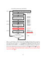
completion of all histories (per stratum), in entry STATS2 of subroutine STATIS.
Linear functions of tallies Often algebraic functions of tallies (sums, products, ratios,....)
are formed after a Monte Carlo run to produce further (post processed) output quantities
(see input blocks 10C and 10E in section 2.10). For those tallies standard deviations are not
available in general, due to statistical correlation between individual tallies obtained from the
same Monte Carlo run.
22
However, for linear functions of tallies (e.g. sums, differences), this is possible even without resorting to the covariance estimators (block 9) of EIRENE. Usually this was done in
“problem specific” modules, e.g. in STATS1 COP for source terms arising in plasma fluid
codes (see section 2.14). In 2012 a new routine (UPFCOP) was added, and is called inside
the particle loop prior to STATS1.
Let a linear function Rlin of default tallies Rk be given by
∑
Rlin =
ak Rk ,
(3.28)
k
(ak are some constant scalar factors) then after each completed history ωi in routine UPFCOP
the sum of contributions
∑∑
∑
∑ ∑
Xk,j (ωi ) =
ak Xk,j (ωi )
(3.29)
Xl (ωi ) =
ak Xk (ωi ) =
ak
k
k
j
j
k
∑
is formed, to finally build the linear function tally Rl (N ) = 1/N i Xl (ωi ) by averaging over
all histories, same as for default tallies. This is possible because in case of linear combinations
of tallies the summation over tallies k and event-contributions j of a single history can be
interchanged (3.29).
Finally the variances for Rl are evaluated in STATS1, reusing the procedure used for default tallies, and the former problem specific routine STATS1 COP for variances from tallies needed for code coupling has hence been made redundant, as indicated in red color in
flowchart (1.12). Currently linear combination tallies Rl are stored on array (tally) COPV.
For them all printout and graphical output options are available. One example of such linear
combination tallies is discussed in section 2.14 for interfacing EIRENE with CFD codes, as
usually the (kinetic) reaction source terms provided by EIRENE to plasma fluid codes are
such linear functions of default tallies.
Statistical independence of MC histories When the Monte Carlo histories from one EIRENE
run are not strictly statistically independent, as e.g. in case of stratified source sampling (see
paragraph below), then a modified formula for the statistical error estimates has to be used.
1.3.3.1
Sampling, Non-analog sampling
One often encounters in literature the description of special, “new” Monte Carlo techniques,
that are greatly superior to so called “standard methods”.
It is true that one can devise very intelligent methods to optimize performance, but each
optimization always only works well for one very particular problem, it can equally well
entirely wreck the performance of an only slightly different case.
For a general purpose Monte Carlo solver for transfer problems, as EIRENE, therefore, no
general advise can be given, although the performance often could greatly be improved by
adapting the method to a particular problem. In particular, non of these “intelligent methods”
have been (and will ever be) hard wired into EIRENE.
EIRENE contains a set of such methods, referred to as “non-analog” methods and controlled
by the flags in input block 9, see section 2.9. Activating those must be accompanied by a very
careful statistical analysis of results, not just the run time per particle, nor even the standard
deviation alone, suffices.
23
We first note here that any random distribution function f (x) arising during the course of generating the chains ω (“particle histories”) can be replaced by another “non-analog” function,
g(x), if a weighting factor,
w(y) = f (y)/g(y)
(3.30)
is included in the formula for the estimator X(ω), y being an actual random number generated
from g. This choice can in some cases increase the efficiency of the algorithm.
The only restrictions on the choice of non-analog sampling functions g(x) (besides practical
ones) are:
if
g(x) = 0,
then f (x) = 0;
(3.31)
and conditions to ensure that the non-analog process remains sub-critical as well.
The condition (3.31) is checked in an EIRENE run whenever non-analog distributions are
applied, and, if violated, an error exit with the message: “violation of Radon-Nikodym condition” occurs.
Note: a violation of condition 3.31 can not be detected otherwise, e.g., by monitoring overflow in the weighting factor w. Of course, values y resulting in a zero in the denominator of
w (equation 3.30) have sampling probability zero according to distribution g(x), and, hence,
are never sampled. Still the results would be biased.
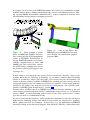
Note: when inspecting an EIRENE geometry plot with particle trajectories (or even a movie:
NLMOVIE=TRUE, input block 1) in order to get an intuitive feeling for the particular transfer
process considered, then all non-analog sampling options must first be turned off, (NLANA
flag in input block 1), for otherwise the pictures may be grossly misleading.
We consider the procedures for random sampling from univariate distributions as known, and
refer to the many textbooks on that, in particular to the “random sampling library” [15]. If
none of the direct methods apply, then still either the non-analog method mentioned above,
or the “rejection method” can be used.
Sampling from a multivariate distribution f (x1 , x2 , ..., xn ) can always be reduced to a sequence of samplings from univariate distributions, by noting that:
f (x1 , x2 , ..., xn ) = f1 (x1 ) · f2 (x2 |x1 ) · f3 (x3 |x1 , x2 ) · ...
(3.32)
Here, f1 is the marginal distribution obtained from f by integrating over all but the first
independent variables. It is a univariate distribution of x1 .
f2 is a conditional marginal distribution obtained from f firstly by integrating f over all but
the first 2 variables x1 , x2 , and secondly then taking the conditional distribution, conditional
on x1 (i.e., the univariate distribution of x2 for given values of x1 ).
Likewise, f3 is a conditional marginal distribution, n-3 fold integration of f , and then distribution conditional on x1 , x2 , and so on.
Random sampling from f (x1 , x2 , ..., x3 ) then proceeds by sampling first x1 from the (univariate) first factor in equation 3.32, then x2 by sampling from the (univariate) second factor, and
so on.
One particular example of this scheme is the “TRIM database surface reflection model” (see
below, section 1.4.2). There, essentially, tables of the conditional marginal distributions mentioned here are pre-computed with the TRIM code. For convenient random sampling, these
tables are stored for the inverted cumulative distribution, i.e., as conditional quantile functions.
24
1.3.3.2
Stratified Source Sampling
The EIRENE code resorts to a “stratified sampling” technique. This technique is one the few
Monte Carlo variance reducing techniques which are quite straight forward, easy to implement and, most importantly, behave in a well predicable way. It is therefore recommended to
always use “source stratification” described below as much as possible. There are, however,
non-trivial issues of load balancing in case of multi-core runs (i.e. Monte Carlo code parallelisation), which are related to assignments of strata for cores, in particular if the average
cpu-time per history strongly varies between strata. In such cases the “proportional allocation of weight” to source strata discussed below is technically difficult to achieve together
together with proper load balancing, due to the stochastic termination of the random walks
in the various strata. Whereas without stratification extracting parallelism seems as trivial as
constructing many independent samples in parallel. This “embarrassingly parallel” feature of
linear Monte carlo transport codes is lost and parallelisation, in combination with stratified
source sampling requires some attention.
Stratified sampling means that the primary source distribution Q(r, v, t) , see Equation (1.1a),
or more generally, for S(x) in (1.1d), can be decomposed into a sum of M independent
sources (this applies for both: the source distribution S itself and the corresponding source
strength s):
M
M
∑
∑
sk
(3.33)
Sk ; s =
S=
k
k
and the solution is obtained by linear superposition of the solutions for each sub-source (“stratum”) Sk . We use again the slightly more general notation S for the inhomogeneous part of
the Boltzmann equation rather than Q, which is the physical source of particles (objects), i.e.
a special case of S.
The stratified sampling technique is a well known statistical procedure from experimental
planning, see any textbook on statistics or Monte-Carlo methods.
It sometimes can significantly affect the efficiency of a Monte-Carlo run. This can go both
ways, depending upon the particular problem and the particular stratification used. Therefore,
as with the non-analog options, no general recommendation can be made.
The effects of source stratification, however, are usually more easy to assess (predict) than
those resulting from general non-analog methods.
In order to make connection with the textbooks, in which “stratified sampling” is often discussed in connection with Monte Carlo integration procedures, the Monte Carlo solution of
the transport problem is interpreted as a Monte Carlo integration, and the “stratified sampling” in Monte Carlo integration becomes a “stratified source sampling” in transport problems in this interpretation. To see this we need to note here only the following (based on
Fredholms alternative for the linear Boltzmann operator):
EIRENE provides estimates of linear functionals (“moments”, “responses”)
⟨g, ϕS ⟩ = ⟨S, ϕ∗g ⟩
(3.34)
As described above, g is the detector function (“weighting function”) ϕS is the solution to
the kinetic transfer equation (Boltzmann equation) in which S was used as (inhomogeneous)
source term. ϕ∗g is the solution of the corresponding adjoint equation, with g as source term
(and S as “weighting function”.
25
The above equation means that EIRENE estimates can simply be regarded as Monte-Carlo
estimates of multi-dimensional integrals, namely of the adjoint function ϕ∗g integrated over
phase space with S defining a distribution (measure) in phase space “µS ”.
It is then obvious that one can split that integral into a sum of integrals by arbitrarily decomposing the domain of integration, i.e., by decomposing the source S into sub-sources
(“strata”) Sk with
∫
M
M ∫
∑
∑
∗
∗
Rg = dx ϕS · g = ⟨S, ϕg ⟩ =
⟨Sk , ϕg ⟩ =
dµSk ϕ∗g
(3.35)
k
k
This is the concept of “stratified sampling”, which, for Monte Carlo particle transfer procedures in particular actually turns out to be a “stratified source sampling”.
Further details about this in our particular context are given in the description of input block
7, section 2.7 below. As pointed out above the evaluation of statistical error estimates has
to account for the stratification, because with stratification the Monte Carlo histories are not
strictly independent anymore.
Grouping the N statistically independent test flights (random samples) into M strata, leads
to Monte Carlo particle numbers Nk sampled from stratum k (i.e., with birth points sampled
only from source Sk ) with:
M
∑
Nk = N
,
Nk > 0
for k = 1, ...M
(3.36)
k=1
where, again, we omit the subscript g for the particular tally (response function) from now
on.
The choice of the Nk is only restricted by the normalization condition in (3.36). This therefore also applies for the allocation of CPU time to individual strata for a given overall CPU
time. This additional freedom can be used in EIRENE runs to affect the statistical error for a
given CPU time. Unfortunately, as with non-analog sampling, this can go both ways. Fortunately, however, here a clear general recommendation can be given, see below in this section:
“proportional allocation”.
˜ k (Nk ) the estimate for tally R as obtained only from the Nk samples from
Lets denote by R
2
stratum k (but scaled with the full source strength s). Likewise, we denote by σ
˜1k
(Nk ) the
˜
variance of estimate Rk per history, i.e. for a single sample, obtained by only using the Nk
samples from stratum k (again implying the scaling with total source strength s). Then clearly
∑ sk
˜ ∗ (N ) =
˜ k (Nk )
R
(3.37)
R
s
k
is the (only) unbiased weighted estimate of R obtained from summing over all strata, i.e.
˜ of R obtained with stratification,
from all N samples. The asterisk denotes the estimate R
˜ ) is the estimate of the same quantity from a simple sample
N = N1 + · · · + NM , and R(N
(no stratification) of same size N :
˜ ∗ (N )} = E{R(N
˜ )}
R = E{R
(3.38)
where E{X} denotes the “expectation value” of random variable X. Furthermore:
σ
˜k2 (Nk ) =
1 2
σ
˜ (Nk );
Nk 1k
∗
σ
˜ 2 (N ) =
26
∑ s2 1
k
2
(Nk )
σ
˜1k
2N
s
k
k
(3.39)
where again the asterisk indicates the value obtained with stratification. The right equation
follows from the sum rule for variances and because the estimates for the strata are mutually
∗
statistically independent. It is clear that the variance with stratification σ
˜ 2 (N ) can certainly
be different from the variance σ
˜ 2 (N ) obtained from a simple random sample (without stratification) of the same size N . To see this we write the trivial identity:
2
σ
˜ (N ) =
M
∑
sk
k=1
s
σ
˜ 2 (N )
(3.40)
For example, in case of “proportional allocation” of CPU-time to strata according to their
source strength sk , i.e., Nk ∝ sk :
Nk =
sk
N,
s
k = 1, 2, . . . , M
one finds from (3.39) for the variance of the stratified sample:
∑ sk
∗
σ
˜ 2 (N ) =
σ
˜ 2 (Nk )
s k
(3.41)
(3.42)
which can be substantially smaller than the variance from the simple sample (3.40) of size
N , if the subdivision into strata is made such that the variability within strata σk2 is less then
the variability in the entire population σ 2 . Furthermore, one can show that with proportional
allocation (3.41) the variance from the stratified sample is always less than or equal to the
variance from the simple sample of same size N , no matter how the subdivision into strata
was done:
sk
∗
If Nk = N ; k = 1, 2, . . . , M then σ
˜ 2 (N ) ≤ σ
˜ 2 (N )
(3.43)
s
i.e., stratified source sampling with proportional allocation is an “inherently safe working
procedure” for variance reduction.
This important inequality can be derived after some lengthy algebra, leading finally to
∗
σ
˜ 2 (N ) = σ
˜ 2 (N ) +
1 ∑
[Rk (Nk ) − R(N )]2
N k
(3.44)
Clearly, the second term on the right side of this equation, which is the variance between
strata, is always positive (or zero) and this fraction of the variance is eliminated from the
Monte Carlo estimate by stratified sampling.
This fact is the reason for the EIRENE option of “proportional allocation of CPU time”
described in input block 7, Section 2.7.
In principle one can even optimize the CPU performance (i.e. minimize the variance per CPU
time, for any given stratification Sk ) by choosing the allocation Nk to strata in an even more
intelligent way (involving a-priori knowledge of the variability within strata σk2 , e.g. estimated
from a previous iteration.) But these options are likely to be quite sensitive to the choice of
the particular tally (response Rg ). In a typical EIRENE application many such responses for a
large variety of detector functions g are estimated simultaneously in one single run. Therefore
this “optimal allocation” schemes are not currently implemented.
27
1.3.4
Source sampling
Source sampling in EIRENE is carried out in routine LOCATE.F. This routine converts uniform random numbers into random numbers with distribution Sk , the k-stratum part of the
inhomogeneous term S. Again sequential sampling (3.32) from conditional distributions is
applied.
In LOCATE.F the following sequence is used (stratum no. istra = k is set in calling program):
S = S1 (x) × S2 (i|x) × S3 (v|x, i)
(3.45)
∑ ∫
with S1 (x) = i d3 vS(x, i, v) being the cumulative distribution of the spatial coordinate
x of the “birth point” of the trajectory, obtained by integrating the source term S over all
velocities and summing over all species. S2 (i) is the distribution of birth species index,
obtained by integrating over all velocities and conditional on the already sampled spatial birth
point. S3 (v) finally is the velocity distribution at the birth-point of the trajectory, conditional
on the already sampled species index i and birth point location x.
This procedure is employed for all types of sources, namely for re-sampling from a stored
“census array” (e.g. initial condition in time dependent mode), for point sources, line sources,
surface sources and volume sources.
If the sampled species i belongs to the background species (i = ib ) rather than to the test
particle species community, then, after completion of sampling from S an appropriate “collision” is carried out (e.g. with a wall surface in case of surface sources), until a test particle
species it results. I.e., formally a sampling from kernel C(x, v, ib → it , ...) is carried out at
the place of birth x to produce initial test particle coordinates.
Stratification of sources has been described in section 1.3.3.2.
1.3.4.1
time-census sources
1.3.4.2
Point sources
1.3.4.3
Line sources
1.3.4.4
Surface-sources
and see special section on “plasma surface recycling source sampling”, 1.5.
1.3.4.5
Volume sources
special case: volume (radiative or threebody) recombination of plasma ions and electrons to
neutrals. Also used for: spontaneous photon emission source in radiative transfer simulations.
1.3.5
Sampling a free flight from the transport kernel T
The conditional sampling distribution T (r′ → r) for the next point of collision (event), given
a test flight is at position r′ , traveling with velocity v′ , is given by (2.11a).
A more intuitive argument for this distribution of free flight path lengths follows from the
simple attenuation law of a mono-energetic beam incident on a thin slab of material, thickness
dl, target material density nt . Clearly the fraction of beam particles undergoing collisions in
28
this slab is σnt dl, with “cross section” σ (stationary target). This results in the attenuation
law
dn = −nnt σdl
→ n = n0 exp(−nt σl)
(3.46)
where n is the number of beam particles, n0 the number of beam particles at l = 0. It is then
naturally supposed that
p(l)dl = [exp(−nt σl)]nt σ(dl)
(3.47)
is the probability for a first collision between l and l + dl, and hence
∫ l
P (l) =
[exp(−nt σl)]nt σ(dl) = 1 − exp(−nt σl)
(3.48)
0
is the corresponding probability distribution function for a first collision at distance ≤ l, i.e.
the same results as derived above formally with the Green’s function argument.
Returning to (2.11a) we first again omit velocity and species index in the argument lists to
keep the notation simple, but we note that certainly the mean free path λ (or macroscopic
cross section Σt ) usually depend explicitly on the test particle energy and species. Let us
introduce the distance of the flight l in direction Ω = v/|v|, hence r = r′ + lΩ, then the
sampling distribution for l is simply
[ ∫ l
]
′
′
T (l) = Σt (r + lΩ) exp −
dsΣt (r + sΩ) , Σt = 1/λt
(3.49)
0
Distances l are readily sampled from this exponential distribution using the inversion method
and the cumulative distribution GT of T
[ ∫ l
]
′
ξ = GT (l) = 1 − F (l) = 1 − exp −
dsΣt (r + sΩ)
(3.50)
0
with ξ (and hence [also 1 − ξ) being a uniformly
distributed random variable on [0,1]. There]
∫l
′
fore, cumulating − 0 dsΣt (r + sΩ) along a flight and comparing it with ln(ξ) with a
uniform random number ξ provides (by inversion) a random sample of the free flight distance
l with the proper distribution.
Sampling the distance l of a free flight, for test particle species “i” with velocity v, from
the transport kernel T requires knowledge of the (“monochromatic”) mean free path λ =
λ(r, |v|) along the trajectory, and, hence, of the “macroscopic cross section” Σ = Σ(r, |v|),
which also may vary along the trajectory.
The “macroscopic cross sections” Σ (by abuse of language, dimension: 1/length) with or
without subscript k (the label for the type of the collision process) or subscript t (for “total”,
the sum over k), are defined as:
Σ=
ν
1
=
,
λ
|v|
λ=
|v|
ν
(3.51)
with the mean free path λ and the collision frequency ν:
ν(r, v, i) = nb ⟨σ · vrel ⟩b ,
vrel = |v − vb |
(3.52)
Here nb and vb are the target particle density and velocity, respectively, and the brackets ⟨...⟩b
denote averaging with the velocity distribution fb (r, vb ) of the background medium species
b.
29
σ is the total scattering cross section, σ = σ(|vrel |).
Hence, e.g., for all isotropic target distributions fb one has:
ν = ν(r, E, ̸ Ω, i)
and
Σ = Σ(r, E, ̸ Ω, i).
Furthermore, let fb be a drifting Maxwellian, with temperature Tb and drift Vb : fb = fb (Tb , Vb ).
Then:
ν = ν(Tb , |v − Vb |, i)
√
Finally, if the thermal speed vbtherm in this Maxwellian: vbtherm =
Tb /mb is very large
compared to typical values of |v − Vb | (i.e.: nearly incompressible flow conditions), then:
ν ≈ ν(Tb , 0, i) = nb ⟨σ · v⟩b
and here ⟨σ · v⟩b is the usual “Maxwellian rate coefficient” for the collision process, taken at
temperature Tb of the background particles (species b) and at zero velocity of the test particles
(species i). For example, in case of neutral atom or molecule collisions with electrons this
approximation is usually valid. From the point of view of electrons or ions, colliding with a
cold background of neutrals or ions (Tb ≈ 0, we have the opposite case: |v| ≫ vbtherm and
then the rate coefficient reduced to the simple product σ(v)v with v being the test particle
velocity.
1.3.5.1
Alternative: fixed time step (or constant path length increment)
If the particle orbit between two events (the Green’s function) is not given explicitly, e.g., not
as simple straight line, then the orbit has to be integrated numerically, using small time steps
∆t or path length increments ∆x. The algorithm to determine the next point of collision then
is different:
After a free flight time ∆t the probability of at least
one collision during this period is the
∫ ∆t
function GT (l0 ) defined above, with |∆x| = l0 = 0 v(t)dt ≈ v∆t the fixed path length
for this step. This follows from the definition of GT as cumulative distribution for the free
flight length (3.50). Clearly 0 ≤ GT (l) ≤ 1 for all positive l, by definition. Lets now assume
constant mean free path λ, and constant velocity v during time step ∆t, and l0 = |v|∆t, to
simplify notation.
The procedure to find the free flight length (or time) is now as follows:
Rather than sampling l by inversion, as in Equation (3.50), now a uniformly distributed random number ξ on [0,1] is compared with the probability GT (l0 ) = 1 − exp[−l0 /λ].
If ξ > GT (l0 ), no collision has happened during this step, and the next step is carried out.
If ξ ≤ GT (l0 ), then at least one collision has happened prior to completion of the step.
Strictly, in this case the exact position of the first collision during this step has to be identified,
by inversion, the time step has to be shortened and the particle has to be moved to the sampled
point of collision in the interval ∆x. However, various approximations are now usually made,
to simplify coding.
• Ignore the fact that more than one collisions could have happened during ∆t.
• replace GT (l0 ) by l0 /λ (= ∆tvΣt (v), see above) when comparing with uniform random number ξ
The second assumption results from Taylor expansion for sufficiently small ∆t such that
l0 /λ ≪ 1.
The first assumption is more difficult to justify generally:
30
If the post collision test particle species is the same and its new velocity is not too different
from that prior to the collision, then the probability for n collisions in the same time ∆t is
roughly Pn = GT (l0 )n and the number of missed collisions in ∆t is
∞
∑
Pi =
i=2
GT (l0 )2
1 − GT (l0 )
(3.53)
For sufficiently small ∆t (and hence l0 ) this error can be made small.
If, however, collisions involve change in species, and/or significant changes in velocity, then
the smallness of l0 /λ must be guaranteed not only for the particle which is currently being considered, but for all particle species in the system and for all possible energies (of
secondaries). E.g.: the excitation cross section for process A → A∗ may be small, hence
l0 /λ ≪ 1 for species A, but the de-excitation (quenching) of state A∗ may be very rapid.
Then the quenching time of species A∗ determines the permitted time-step for species A in
this approximate procedure. Other critical examples may be systems composed of both rather
stable chemical species and short living radicals, e.g hydrocarbons.
The EIRENE code therefore only uses the correct full sampling procedure (3.50), even when
particle orbits (e.g. of ions) are integrated numerically with time-steps.
1.3.6
Sampling from the collision kernel C
The general rules for sampling from multivariate distributions outlined in Section 1.3.3, Equation (3.32) also apply here.
It is not necessary, but usually most convenient and intuitively most clear, to decompose
the kernel C according to the physical nature of the various collision processes taken into
account.
The collision kernel C was written as (see equation 2.9)
∑
Σk
pk Ck (r′ ; v′ , i′ → v, i) , pk =
C(r′ , v′ , i′ → v, i) =
Σt
k
with summation over the index k for the different types of collision processes under consideration and pk defined as the probability for a collision to be of type k. The normalizing
factor
∑∫
1
′
dv Ck (r′ , v′ , i′ → v, i) , Ck = Ck
ck (x ) =
ck
i
was the mean number of secondaries for this collision process. The function Ck then is a
conditional probability density for (v, i), given the pre-collision coordinates (r′ , v′ , i′ ).
Sampling from C (given that a collision of some kind has occurred) proceeds most conveniently by firstly sampling the type k of the process from the discrete distribution
(pk ,
k = 1, .., K),
and then by sampling the post-collision state of the test-particle from Ck . Finally the weight of
the test-flight after collision is increased (or reduced) by multiplying it with the normalization
constant ck .
The decomposition of C into sub-kernels Ck is somewhat arbitrary, and the criteria may also
be computational aspects rather than the different physical nature of the various processes
taken into consideration.
31
Sampling (v, i) from Ck can be done along the same idea: first factoring out the discrete distribution for the species index i, and then by sampling v from Ck,i , the conditional distribution
for v given the type of the process is k and the species of the post collision trajectory is i. Let
(nk,i′ ,∑
i′ = 1, ..., Ik ) be the number of post collision particles of species i′ from process k, and
nk = i′ nk,i′ . Then
(˜
nk,i′
i′ = 1, ...Ik ) = (nk,i′ /nk ,
i′ = 1, ...Ik )
is the discrete distribution for the post-collision particle species i′ , given a collision process
of type k.
1.3.7
elastic collisions
1.3.8
charge exchange
1.3.9
electron-impact collisions
1.3.10
general heavy-particle-impact collisions
1.3.11
photon processes (emission, absorption, scattering)
32
1.4
Surface Reflection Models
Within the terminology fixed in section 1.2 the effects of the interaction of neutral particles
(and escaping ions) with surfaces surrounding or inside the computational volume can be
described by additional boundary conditions. It is, however, much more convenient for Monte
Carlo applications to describe this interaction as just one special type of collision process in
the collision kernel C of equation (2.9), i.e. as
∑
C = pw · Cw +
pk Ck ,
(4.54)
k
with pw (r) = 1, if r is a point on a surface, and pw (r) = 0 elsewhere. The transport kernel
T can be modified such that the maximum length lmax for free flight to the next point of
collision is the distance to the nearest surface along the track of the particle. The reflection
kernel Cw is further decomposed it into a kernel Cwf (fast particle reflection), Cwt (thermal
particle re-emission) and Cwa (particle absorption) with respective probabilities, pf , pt and
pa , such that
Cw = Cwf + Cwt + Cwa = pf Cwf + pt Cwt + pa Cwa ,
pf + pt + pa = 1.
(4.55)
Here C are, as above, the normalized versions of the collision kernels C.
We discuss in detail only the fast particle reflection model Cwf since Cwt is generally a
mono-energetic and cosine angular distribution or a Maxwellian flux distribution at wall temperature, and Cwa only describes the transition into the “limbo state” xa “absorbed particle”.
It is usual in neutral gas models to replace Cwf with numerical or analytical fits to moments
of Cwf , e.g., such as the particle and energy reflection coefficients CP and CE . The particle
- wall interaction is often supplemented by simple assumptions on the angular distribution
(cosine or specular) of the particles leaving the surface.
One has for the particle reflection coefficient:
∑∫
dv Cwf (r; v′ , i′ → v, i)
(4.56)
CP =
i
Note that CP = pf = cwf in the terminology of equation 2.10.
The energy reflection coefficient is defined as:
∫
1 ∑
1
CE = ′ ·
dv E · Cwf (r; v′ , i′ → v, i) = ′ · C˜E
E
E
i
(4.57)
¯ ′ · CP , with E¯
Here E = mv 2 /2 is the energy of the reflected particle. Hence CE = E/E
denoting the mean energy of the reflected particles.
1.4.1
The Behrisch matrix reflection model
One model, the matrix model due to Behrisch [16], is hardwired in EIRENE (and in many
other codes such as AURORA, BALDUR, TRANSP). This model has been used as a standard
option in many benchmarks [17]. The model is based upon a table of values for CP⊥ (E ′ ) and
a stochastic matrix B ⊥ for the transition E ′ → E, for H atoms striking a stainless steel target
33
at normal incidence. For other incident angles ϑin the moments are modified in EIRENE by
the relations:
CP (ϑin ) = 1 − (1 − CP⊥ ) · cose1 (ϑin )
(4.58)
and
CE (ϑin ) = 1 − (1 − CE⊥ ) · cose2 (ϑin ).
(4.59)
This latter moment equation can be satisfied by modifying the tabulated stochastic matrix
B ⊥ (E ′ → E) in many different ways. In EIRENE, we first sample E from B ⊥ (given E ′ )
and then set
E = E ′ − (E ′ − E) · cose2 (ϑin ).
(4.60)
¯ ′ · CP (ϑin ) = CE (ϑin ), with
The linearity of E in E gives an expectation value E¯ with E/E
CP and CE as given by equations (4.58) and (4.59), respectively.
To describe the angular distribution of re-emitted particles, let ex , ey , ez define an orthonormal basis at the strike-point of a test-particle on a surface. Here let ex be the unit vector
parallel to the outer surface normal and let the incident particle travel in the local xz-plane.
Furthermore, let ϑr and φr be the polar and azimuthal angles sampled from a cosine distribution around −ex . The speed unit vector Ω of the reflected particle in EIRENE is then given
by
Ωx = − cos(ϑˆr )f1 (ϑin ) + sin(ϑˆr ) sin(φr )f2 (ϑin ),
Ωy = sin(ϑˆr ) cos(φr ),
Ωz = sin(ϑˆr ) sin(φr )f1 (ϑin ) + cos(ϑˆr )f2 (ϑin ),
(4.61)
with
sin(ϑˆr ) = f1 (ϑin ) sin(ϑr ),
f1 (ϑin ) = cose3 (ϑin ),
1
f2 (ϑin ) = (1 − f1 · f1 ) 2 .
In total we have defined three parameters e1, e2, e3. The first two parameters e1 and e2 account for particle and energy reflection coefficients that continuously increase with incident
angle (recommended: e1=1, e2=0.5 from comparison with TRIM code calculations, see below).
The third parameter e3 can be used to take into account an increasing contribution of specular
reflection at near grazing incidence. e3=0 gives a pure cosine distribution, e3=1 reproduces
the distribution given in [13]. In general this model describes a fraction of specular versus cosine reflection which increases with ϑin , and in the (purely mathematical) limit of ϑin = 90◦ ,
pure specular reflection. Furthermore, the parameter e3 controls the speed at which the specular part aspec (Ω) of the angular distribution a(Ω) = aspec (Ω) + acosin (Ω) increases with
ϑin .
The interaction of neutrals and ions with a solid surface for target-projectile combinations
other than H onto stainless steel are modelled using a reduced energy scaling.
1.4.2
TRIM code database reflection models
Complementary to the surface model described above, EIRENE is coupled to computer generated reflection databases, produced with the TRIM code (see references [18] and [19]). At
34
present a discretized form of the reflection kernel Cwf , including all correlations between the
vector components of v′ and v, is available for the target-projectile combinations listed in
table 1.1. ZNML is a target material flag set for each surface in the input file, blocks 3a and
3b, and is described below in block 6b, “Data for local reflection models”. These databases
are, essentially, tables of conditional quantile functions obtained from large random samples
of test particle trajectories in the solid.
Table 1.1: Surface reflection database (TRIM Code)
No
1
2
3
4
5
6
7
8
9
10
11
12
13
14
15
16
17
18
19
20
Projectile
H
D
H
D
He
He
T
T
D
He
H
T
D
D
Ne
Ne
H
H
T
He
Target ZNML
Fe
5626.
Fe
5626.
C
1206.
C
1206.
Fe
5626.
C
1206.
Fe
5626.
C
1206.
W
18474.
W
18474.
W
18474.
W
18474.
Be
904.
Mo
9642.
C
1206.
Be
904.
Cu
6429.
Mo
9642.
Mo
9642.
Mo
9642.
We consider these “database -” reflection models to be the most complete option available
at present and recommend to further extend the databases to additional projectile - target
combinations, and in particular to sputtering and self-sputtering data (such as, e.g., C onto C,
or Be, etc.).
For an INTOR benchmark case for neutral particle Monte Carlo Codes [17] the choice of
a particular surface reflection model had no strong impact on the results. This was shown
by running the EIRENE code with all three models (“Behrisch Matrix”, TRIM database and
MARLOWE database (at that time available as a third option. Meanwhile the MARLOWE
database is not available anymore).
It was found that this had little influence on global parameters as, e.g., the pumping efficiency
for the particular geometry (5.4 %, 5.3 % and 5.2 % respectively.). On the other hand, it can
easily be imagined that in other cases (different plasma conditions, more detailed geometries)
the choice of the reflection kernel Cwf can be more important for the result. Certainly in
all cases, in which the results are sensitive to the neutral particle velocity distribution near
35
surfaces, details of the reflection kernel matter. This is, for example, the case for computed
line shapes of certain electronic transitions (Hα lines etc.), see e.g., reference [20].
36
1.5
Recycling surface sources
It has been found (mid eigthies of last century: within INTOR framework) as a result of
benchmark calculations with several different neutral gas transport Monte Carlo codes (EIRENE,
DEGAS, NIMBUS, DDC83) on the same input data that the main divergence in the results
from the different codes tested was due to different primary source terms Q in the transport
equation [equations (1.1a,1.1b) and (1.6a)] , although target fluxes and temperatures had been
prescribed to be identical. Here we describe one particular EIRENE surface source option in
detail. The way the source is modelled by EIRENE allows consistency with kinetic boundary conditions for plasma fluid equations at plasma facing surfaces. To describe this, we first
write the volumetric source Q (particles per unit time and per unit (r, v)-phase space volume)
in terms of a surface flux Γw and a surface delta-function. The surface (wall) flux Γw thus has
dimension: particles per unit time, per velocity space unit, and per unit area:
Qw (r, v, i) = Γw (r, v, i) · δw (π),
(5.62)
where π is a coordinate normal to the surface Sw : π(r) = 0, i.e.: eπ = ∇r π(r), pointing
away from the computational volume. We see that Γw specifies the (ingoing) “transport” flux
Φ introduced in (1.6a) at the boundary of the computational domain. We will henceforth use
the notation Γ rather than Q, in case of surface sources. Γw is a kinetic (microscopic) surface
source (flux-) density distribution, backward directed (into the computational volume, i.e.,
only vπ < 0).
To convert from a forward directed ion flux distribution ΓSh,ion (v) at the plasma-sheath interface SSh to a neutral flux distribution back from the wall surface Sw , we fold ΓSh,ion with
a (magnetic plus electrostatic) sheath transmission kernel TSh and with the surface reflection
(incl. sputtering) kernel Cw , equation 4.54:
∑∫ ∫ ∫
d3 r′ d3 v ′ d3 v ′′ ΓSh,ion (r′ , v′′ , i′ )
Γw (r, v, i) =
i′
·TSh (i′ ; r′ , v′′ → r, v′ ) · Cw (r; v′ , i′ → v, i)
(5.63)
The summation over i′ is performed over all ion species entering the sheath region.
A typical example for ΓSh,ion is at least sonic parallel plasma flow (Mach number M∥ ≥ 1
along the magnetic field lines) entering the magnetic pre-sheath. In this magnetic pre-sheath
the ion trajectories are bend over (accelerated by the electric pre-sheath field) such that at the
entrance of the electrostatic sheath at least sound speed is already reached with respect to the
surface normal: Mπ ≥ 1.
A commonly adopted simplification is made by ignoring the typically small spatial volume
between the plasma sheath interface and the wall surface. Hence: TSh factorizes into a 3D
delta function δ 3 (r − r′ ) and a deterministic transition kernel for the velocities v′′ → v′ .
Random numbers from Γw are generated conveniently by sampling, firstly, (r′ , v′′ , i′ ) from
ΓSh,ion , next generating (r, v′ ) from TSh and then, finally, (v, i) from the conditional distribution Cw , the weights, velocities and species indices of re-emitted (neutral) particles.
A frequently employed assumption for ΓSh,ion is a one sided (only positive velocity components into the sheath) forward drifting Maxwellian ion flux distribution at the interface
between plasma and electrostatic sheath SSh . In this case the bending of trajectories from
parallel (to B) to normal (to the surface) sonic flow within the magnetic pre-sheath is already
37
included in ΓSh,ion , e.g., via boundary conditions in a CFD model for plasma ion flow, and
the action of operator TSh is solely the acceleration in the electrostatic sheath.
Alternatively, and in cases when the magnetic field is tilted with respect to the wall surface,
one may define ΓSh,ion (v) to be the kinetic transport flux distribution entering the magnetic
pre-sheath, i.e. with a drift velocity of at least ion sound speed in the direction parallel to
the magnetic field B (rather than normal to the wall). In this case the action of the magnetic
pre-sheath must be accommodated in the sheath kernel TSh , which we might even consider
to split into a magnetic pre-sheath (MP) kernel and an electrostatic sheath (Sh) kernel:
TSh = TM pSh (rM pSh , vM pSh → reSh , veSh ) · TesSh (reSh , veSh → wall)
CFD
(5.64)
kinetic
magn. pre-sheath
B
sheath
σ
Γi
ΔΦ
Vi
p
j = ji + je
MP
W
Sh
Figure 1.1: Transition region between fluid plasma (CFD) and wall surface, schematic. The
plasma flow is specified by CFD models at the entrance surface of the magnetic presheath
⃗
MP (taken normal to the magnetic field B)
1.5.1
half-sided Maxwellian flux at electrostatic sheath entrance
One of the standard options in EIRENE, in particular in applications in which EIRENE is
coupled into a plasma fluid code, is a half sided forward drifting Maxwellian ion flux distribution (options: NEMODS=6,7, Section 2.7). The kinetic plasma ion flux distribution
entering the electrostatic sheath is given as
(
)
1
1
0
2
ΓSh,ion = 2 · vπ · exp − 2 (v − Vd ) , vπ > 0
(5.65)
α
2vTi
√
with vTi = kTi /mi , the thermal ion velocity, normalizing constant α2 and with the drift
velocity Vd . See Section 2.7 for a description of related EIRENE input flags. The superscript
38
0 indicates normalization of the flux to one particle per unit time and unit area:
∫
d 3 v Γ0Sh,ion (v) = 1
(5.66)
vπ >0
Consider now the three orthogonal velocity components v1 , v2 , v3 chosen such that v3 = vπ ,
i.e. the v3 velocity component is normal to the surface (target), and hence also normal to the
plasma-sheath interface. Γ0Sh,ion (v) factorizes in the three uni-variate distributions
Γ0Sh,ion (v) = Γ0Sh,ion,1 (v1 ) · Γ0Sh,ion,2 (v2 ) · Γ0Sh,ion,π (vπ )
(5.67)
The first two factors here are simply (shifted) Gaussians and sampling random velocities
v1 , v2 from them is trivial (e.g.: Box Muller method), whereas the third factor is a one-sided
drifting Maxwellian flux distribution:
(
)
1
1
0
2
ΓSh,ion,π (vπ ) = 2 · vπ · exp − 2 (vπ − Vd,π ) , vπ > 0
(5.68)
απ
2vTi
The normalizing factor απ2 for this distribution of the normal component vπ reads:
απ2 = vT2i · exp(−Vπ2 )g(Vπ ),
(5.69)
√
√
with Vπ = Vd,π /( 2 · vTi ) and g(x) = 1 + π x [1 + erf(x)] exp(x2 ).
(Note that the dimensionsless velocity V introduced here is related to the Mach number M
by
√
√
Te /Ti + 1
Te /Ti + 1
V
V
√
√
=
=M
(5.70)
V=√
cs
2 vTi
2
2
√
with the (isothermal) ion sound speed cs defined as: cs = (Te + Ti )/mi . Hence V = M
only if Te = Ti .
It is clear that random sampling the π-component vπ of v from Γ0Sh,ion,π is not trivial even
for this seemingly simplest sheath entrance ion velocity distribution, because the cumulative
distribution function F of a 1D forward drifting Maxwellian (with cut-off at vπ = 0):
∫ vπ
F (vπ ) =
dvπ′ Γ0Sh,ion,π (vπ′ )
(5.71)
0
cannot be inverted explicitly.
Therefore in the EIRENE code we apply the Monte Carlo “biassed source sampling” concept, (module: VELOCS.F). We sample this component v˜π from a “non-analog” truncated
˜ 0 (˜
Maxwellian flux distribution Γ
vπ ) (see Section 1.3, paragraph 1.3.3.1 above) with zero drift
in π-direction but with different “non-analog” π-temperature T˜π,i , (T˜π,i ̸= Ti , V˜d,π = 0).
Note that although this non-analog distribution clearly violates any “Bohm criterion”, it is,
taken together with the weight correction factors described below, unbiased and a fully legitimate sampling distribution because it fulfils the “Radon-Nikodym condition” (3.31). Sampling from this non-analog distribution can be done by setting, e.g.,
√
v˜π = α
˜ π · − ln(ξ) · 2, (note: α
˜ π = vT˜π,i ,
since V˜d,π = 0),
(5.72)
ξ being a uniformly distributed random number between 0 and 1.
39
In order to find the weight correction factor associated with this non-analog procedure, we
first note that
V˜π = 0,
α
˜ π = vT˜i
This gives the following result for the weight correction factor w(˜
vπ ), see equation (3.30), to
be applied for each sampled non-analog velocity component v˜π :
(
(
))
Γ0Sh,ion (˜
vπ )
T˜π,i
v˜π Vd,π
v˜π2
Ti
1
w(˜
vπ ) = 0
=
exp
− 2 1−
·
. (5.73)
2
˜
˜
Ti
vT i
2vTi
g(Vπ )
ΓSh,ion (˜
vπ )
Tπ,i
This non-analog sampling of the source term introduces additional statistical fluctuations in
the results, since the initial test particle weights fluctuate with variance
(
)
∫ ∞
2V
1
π
2
2
0
˜ Sh,ion (˜
σ (w) =
d˜
vπ w (˜
vπ ) · Γ
vπ ) − 1 = g √
/g(Vπ )2 ·
−1
(2 − b)b
b
0
(5.74)
where b = 2 − T /T˜. We use the ansatz b = C · Vπ + 1 and compute numerically that value
of C which minimizes σ 2 in the range 0 ≤ Vπ ≤ 1. We find C = 0.6026. This means that the
ratio of the “real” temperature Ti and the non-analog temperature T˜π,i should be chosen to be
Ti /T˜π,i = 1 − 0.6026 · Vπ . This choice optimizes the statistical performance. In principle, of
course, any other T˜π could have been used without introducing bias into the algorithm.
The mean energy of ions generated by this sampling procedure is (note: the distribution Γ0 is
already normalized to flux one):
∫ ∞∫ ∞∫ ∞
mi
2
E(Vπ , Vσ ) =
·
d3 v ′ v ′ · Γ0Sh,ion (v′ ) =
2
−∞ 0
∫−∞
∫ ∞
∫ ∞
∞
mi
·
dv1
dv2
dvπ (v12 + v22 + vπ2 ) · Γ0Sh,ion (v′ ) (5.75)
=
2
−∞
−∞
0
= Ti · γE ,
with the half sided integration for the π-component of v, and:
[
]
g(Vπ ) − 1
2
2
γE = 2 + Vσ + Vπ + 0.5 ·
,
g(Vπ )
(5.76)
Here we have decomposed the drift velocity Vd into a normal (to the surface) π-component
Vd,π and a σ-component Vd,σ parallel to the wall surface.
Vσ =
|Vd,σ |
|Vd − Vd,π |
√
=√
.
2 · vT
2 · vT
(5.77)
Note that for Vπ = 0 this reduces to the expected formula γE = 2 + Vσ 2 . Furthermore, if
Vσ = 0 (normal incidence) and Vπ → 1 (i.e. for the Bohm sheath condition Mπ → 1 in case
of Te = Ti ), then γE for the forward sided fluxes approaches the value for total heat fluxes
from drifting Maxwellians: γE = 2.449 + Vπ 2 ≃ 52 + Vπ 2 , as it must.
We conclude that the above scheme is both an accurate and efficient random number generator
for truncated shifted Maxwellian flux distributions of particles incident onto or emitted from
˜ with the weight w(˜
surfaces. Of course, after having generated v
vπ ) and before reflecting
the particle via the kernel Cw , the acceleration of an ion in a sheath potential in direction π
(normal to the target surface), as formalized in the sheath transmission kernel TSh mentioned
above in Eq. (5.63), can easily be included.
40
1.5.2
The electrostatic sheath
The electrostatic sheath potential in front of a target surface is derived from assuming a given
net electrical current jpl and a known ion particle current Γ+ (i.e., j + = qi Γ+ electrical ion
current entering a plasma-target boundary layer (the “sheath”), with qi = eZi being the ion
charge, e the elementary charge and Zi the ion charge number) flowing over the target sheath
edge. Both these currents, and the electron current j − = qe Γ− = −eΓ− , are taken to flow
parallel to the B-field at the plasma-sheath edge (more generally: forming an angle Ψ ̸= 90
degrees with the target surface normal π).
Often, but not necessarily, it is assumed: jpl = j + + j − = 0, i.e., locally ambipolar flow
conditions.
We start with a Maxwell-Boltzmann density distribution ne (x) for the electrons, with electron temperature Te , in the electron retarding electric field with potential Φ(x). Here x is a
coordinate parallel to the current flow, e.g. the magnetic field B. The electron current density
along the field is then (after reduction, possibly, due to secondary electron emission):
√
8kTe
−
av
jT = −e·1/4·ne,T ·ve ·(1−γs.e.e. ) = −e·1/4·ne,S ·exp[e∆ΦS,T /kTe ]·
·(1−γs.e.e. )
πme
Here γs.e.e. is the secondary electron emission coefficient and veav is the average electron
velocity. The subscripts S and T stand for the plasma-sheath interface and for the target
surface, respectively and ∆ΦS,T is the (typically negative) voltage drop from the plasma
sheath edge to the target.
In order to determine the sheath voltage drop ∆ΦS,T we equate the component normal to the
target of this current density with the corresponding component of the net ion current density:
( −)
(
)
−jT π = −jT− · cos(Ψ) = (jT+ − jpl ) · cos(Ψ) = jT+ − jpl π
Hence the cosine of the angle Ψ of direction of current flow (e.g. of field line inclination
against the target surface normal, if the current flows parallel to B) cancels out, as does the
elementary charge e. The ion electrical current to the target jT+ (= (jS+ )π , no ion sources
within the sheath region) is given as
∑
∑
jT+ = e
Zi · ni,S · Vπ,i,S = e
Zi · ni,S · Mπ,i,S · ci,S .
i
i
The sum is over all ion species, Zi is the charge state of species i, ni,S is the corresponding
ion density and Vπ,i,S the ion flow velocity component normal to the target, of ion species i.
Mπ,i is the Mach number of the corresponding current component, and ci is the ion acoustic
speed for species i.
Hence, combining the three previous relations, the sheath potential difference ∆Φ in terms
of given jpl , Te , γs.e.e. and ions flows Γi , reads (omitting the subscript π for the components
41
normal to the target in these quantities):



√
(
)
√
∑
ni,S
jpl
2π
me

√ 
e∆Φ/kTe = ln 
Zi
· Vi,S
−
(1 − γs.e.e. )
n
kT
e
e,S
e
e · ne,S · kT
i
me
(5.78)


√
(
)
√
∑
2π
ni,S
me
jpl

√ 
Zi
= ln 
· Mi,S · ci,S
−
(1 − γs.e.e. )
n
kT
e
e,S
e
e · ne,S · kT
i
me

(5.79)
This expression (5.78) is evaluated by the function SHEATH of the EIRENE code, taking
local plasma data for Te and ni and Vπ,i (ne from quasi-neutrality) at the point of impact of
an ion at a wall boundary (e.g., the divertor target plate), strictly: at the sheath entrance S in
front of the target.
Special forms of (5.79) are often quoted in the literature. Writing for the ion acoustic speed
ci explicitly
√(
)
γkTi + kTe
ci =
mi
(γ denoting the adiabatic coefficient) and hence:
√
ci ·
me
=
kTe
[(
)
]1/2
γkTi
me
+1 ·
kTe
mi
(5.80)
we recover well known expressions for simpler cases. Consider, e.g., a single ion fluid case,
ne = ni = n, with Zi = 1, and Mi = 1 (Bohm sheath condition for isothermal flow, γ = 1),
(5.79) reduces to:


√
( √
)
2π
me
jpl
√ 
e∆Φ/kTe = ln 
ci,S
−
(1 − γs.e.e. )
kTe
e · n · kTe
me
(5.81)
√
[(
)
]1/2 (
)]
2π
γkTi
me
jpl
= ln
+1 ·
1−
(5.82)
(1 − γs.e.e. )
kTe
mi
e · n · ci,S
[
the latter equality (5.82 follows after insertion of (5.80) into the former.
If we let, furthermore, the net electrical current be zero: jpl = 0 and zero secondary electron
emission γs.e.e = 0, we then find the classical result:
[
(
)]
1
2πme Ti
e∆Φ/kTe = ln
+1
2
mi
Te
Hence, e.g., for a pure hydrogen plasma, and for Te ≈ Ti , we have e∆Φ/kTe ≈ −2.5 and
≈ −2.84 for a pure deuteron plasma.
42
1.5.3
The magnetic pre-sheath
In most situations when EIRENE is applied to plasma surface interaction studies the ionplasma flow velocity Vi is predominantly parallel to a B field: V∥,i ≈ |Vi |, and it is this parallel ion flow velocity, which is usually available from CFD plasma simulations, via boundary
conditions specified for the momentum balance equation at the entrance of the magnetic presheath (M P ) rather than at the entrance of the electrostatic sheath S.
The sheath model of EIRENE then is supplemented by a model PRE-SHEATH for the transition of currents and Vi,M P to Vi,S , i.e. in particular to derive the currents jπ,S and flow
components Vπ,i,S entering the electrostatic sheath from jM P and Vi,M P
to be written....
43
1.6
Combinatorial description of geometry
EIRENE is a Monte Carlo Code. Defining geometry in a Monte Carlo code is complex and
laborious.
Of the three typical options for definition of the target geometry in Monte Carlo Codes:
• “Constructive solid geometry (CSG)”,
• “boundary representation (BREP)”
• “Voxel Geometry”
EIRENE uses a combination of the latter two concepts.
In CSG a solid object is “constructed” from the intersection, union or other boolean operations of several “half-spaces”. Each half space in specified by a relation F (x, y, z) ≤ 0,
typically F is a low order polynomial. For example the neutronics code MCNP used e.g. for
ITER nuclear safety studies, is based on CSG.
In BREP geometry, surfaces and volumes are build up from constituent parts. These parts
may be related with algebraic functions (elementary BREPs) or complex functions such as
Bezier functions or B-splines (advanced BREPS). Most CAD software uses BREPs in their
native definition of geometry.
In the EIRENE BREP options surfaces are build from (bounded) algebraic functions. These
surfaces are referred to as “additional surfaces”, see Section 2.3.2. EIRENE uses only algebraic functions, up to second order (some extensions to raise the order to fourth order have
been started recently but are not ready to use).
In “Voxel geometry”, a 2D or a 3D object is constructed from identically shaped volume elements (“voxels”). In EIRENE these may be triangles or quadrangles in 2D, or tetrahedrons
in 3D. New options to accommodate trilinear hexaedra as 3D voxels are currently being developed in connection with 3D edge codes such as EMC3. The bounding surfaces of these
voxels are referred to as “standard grid surfaces” in EIRENE, see Section 2.2. These volume
discretisation meshes (VOXELS) can be read into EIRENE from external files. For example
the mesh in B2 CFD plasma fluid code is read into EIRENE directly from the CFD grid generator in coupled B2-EIRENE applications. Wall meshes are build from these by assigning
a surface reflection model to some of the (voxel-) surfaces (Section 2.3.1), whereas internal
(grid-) surfaces remain transparent for flow of test-particles.
Note added in 2008:
An attempt has been made in 2008 to use CAD files directly for 3D wall surfaces. This was
done via the already existing CAD-MCNP interface. We had then tried to turn the CSG input
for MCNP (see above) into a BREP form for EIRENE. In principle this works. But in practice
the de-tour via the CSG concept leads to prohibitively complex BREP input for EIRENE.
A direct CAD-BREP interface seems now much more efficient to us and more natural anyway, and has meanwhile (2011) been established by an intermediate code step (the ANSYS
code), which first converts CAD output into a triangulation of surface elements, and then each
triangle (in 3D space) is taken as “additional surface” (BREP concept) into EIRENE. Very
large sets of triangles required optimisation procedures, which have also been implemented
(in EIRENE module timea.f) on the basis of OCTREE concepts adopted from ray-tracing
procedures used in image processing.
44
A complete set of surfaces in an EIRENE geometry may consist of a combination of both:
standard surfaces (hence: defining standard grid cells, (voxels), and additional surfaces, defining a general BREP discretisation (additional cells). A more complicated situation arises
when additional surfaces intersect standard grid voxels.
Figure 1.2:
Early example a combination of BREP and VOXEL discretisation, around 1985 for ALT-II pumplimiter
studies at TEXTOR. Discretisation inside the TEXTOR tokamak vessel (torus):
VOXEL, supplemented by about 100
(BREP) first and second order surfaces
for ALT-II scoops, pumping ducts and inner structures such as probe supports, getter pumps, etc..
Figure 1.3:
same as left Figure, but
BREP part only, and EIRENE re-run with
more modern 3D visualisation graphics
program, 2009
If these surfaces are transparent, they can be used to conveniently “measure” fluxes at any
position. But if they are reflecting, or absorbing, e.g. to define a complex shaped bounding
surface in an otherwise simple grid, then some care is needed because the automatic cell
volume evaluation, which is available in EIRENE for standard grid cells (voxels), may not
correspond anymore to the cell volume accessible for test particles. Cell averaged quantities
(divided by cell volume) may then not necessarily be scaled properly. For a possible workaround see NLERG option in input block 1, section 2.1.
From the above it follows than in an EIRENE model surface elements building up the wall
can be defined as bounded algebraic surfaces, with triangles as special case, i.e. as “additional
surfaces, BREP”, or can be bounding surfaces of the voxels, if the “grid of voxels” extends
up to the real wall, or a combination of both.
As can be seen from the flowcharts, all the geometrical calculations needed for tracing test
flights and for estimating volume- and surface averaged tallies are compiled in a “geometry
block”, which can easily be exchanged. In most cases (e.g., all installations of EIRENE
outside FZ-J¨ulich) we load the most complete, fully 3D block “GEO3D”, which allows fully
45
3 dimensional spatial resolution. Lower dimensional (0D, 1D or 2D) are contained as special
cases, e.g. by choosing only grid surfaces with proper symmetry.
There is, in general, not a very large CPU benefit from running EIRENE with simpler specialized and geometry optimized blocks such as GEO2D or GEO1D for 2D or 1D models,
respectively, because the saving in CPU costs in most cases is only around 10 - 20 %, so these
options have not been supported since the late eighties of the last century anymore.
The geometry module of EIRENE
The following operations have to be executed by the block:
Suppose the three dimensional computational volume is discretized by a mesh of n surfaces
Si , i = 1, 2, ..., n . Each of these surfaces is defined by a set of Λi equations (unbounded
surfaces):
λ = 1, 2, ..., Λi ,
(6.83)
fλi (x, y, z) = 0,
and, optional, for each unbounded surface λ a subset of Πλ inequalities (e.g. for turning the
unbounded surfaces into finite segments):
i
gλ,π
(x, y, z) ≤ 0,
π = 1, 2, ..., Πλ .
(6.84)
This means that for all unbounded surfaces Si,λ only the points, which fulfill all corresponding
inequalities (6.84) are regarded by EIRENE as valid parts of the finite surface element.
Assume a test particle at position r0 = (X0,Y0,Z0) moving with speed unit vector Ω0 =
(VELX,VELY,VELZ). The block then has to provide the nearest intersection r1 of the straight
line (“sample trajectory”)
G(t) : r0 + tΩ0
amongst all possible intersections with the surfaces Si . Moving the “particle” from r0 to r1
and then repeating the block until the total track length l as sampled from the transport kernel
T (l) (2.11a) is reached, allows to generate histories with all information available along the
track to evaluate the estimators mentioned in section 1.2.
In EIRENE f and g are general 2nd order (with linear surfaces as special case) algebraic
equations of the form
h(x, y, z) = a0 + a1 · x + a2 · y + a3 · z + a4 · x2 + a5 · y 2 + a6 · z 2 +
+ a7 · xy + a8 · xz + a9 · yz
(6.85)
Hence in the geometrical block nothing else but second order equations
t2 + p · t + q = 0
have to be solved accurately and as efficiently as possible. We note in passing that each of
this surfaces may be transparent, purely absorbing, semi transparent or (partially) reflecting.
Surface sources may be defined on each surface. These surfaces may be “invisible” from
one side and transparent, absorbing or reflecting from the other and each surface can “operate
switches” if intersected by a test flight, such as abandoning the evaluation of atomic or molecular reaction rates (entrance into vacuum regions) along the flight, abandoning evaluation of
volume averaged responses (e.g., in some uninteresting regions) or abandoning geometrical
calculations (for those surfaces, for which it can be known a priori that they will not intersect
a flight path originating at a particular surface or in a particular cell).
46
1.7
time dependent mode of operation
The section is currently rewritten. Please refer to the J.Nucl.Mater. paper: D.Reiter et al., Vol
220-222 (1995), 987-992.
Details of options available in EIRENE for time dependent problems are also given in Section
2.13.
The following issues have to be considered in case of time-dependent coupling schemes to
external plasma fluid solvers, see figure 1.6:
The coupling is explicit, hence CFL-type conditions for the time-step have to be obeyed.
Here this means: the time-step must be shorter than the time between re-ionization and subsequent neutralization (in the volume or at the targets), because the fate of a particle during
its intermediate ionized phase is not included in the explicit Monte Carlo procedure.
The noise level for collision estimators increases with smaller time-steps. Hence: avoid all
collision estimators in t-dependent mode.
Please contact us for an update on this situation, if you wish to use that option.
47
1.8
non-linear effects: coupling to plasma fluid models
The section is currently rewritten. Please refer to the report J¨ul-2872, Feb 1994, by G.Maddison
and D.Reiter for details (ref. [10]).
The back-reaction of the host medium (plasma) on the neutral (test) particle kinetics renders
the combined plasma-neutral transport problem non-linear already for the Monte Carlo solution of the “linear” Boltzmann equation. This non-linearity is not in the collision integral, but
in the dependence of the collision parameters (collision rates, mean free pathes, ...) on the
plasma parameters. It can be dealt with by iterating a solver for the host medium (plasma)
and for the kinetic equation (neutrals). Such a CFD solver for 2D plasma flows is e.g. the
B2-“BRAAMS” code, and its iterative coupling to the Monte Carlo kinetic code EIRENE
was developed in the late eighties and early nineties of the last century, under NET-KFA contracts, involving three EFDA associates: the EIRENE group at FZ J¨ulich (formerly KFA), the
CCFE (formerly AEA Culham) edge modelling group as well as ERM Brussels.
The historically oldest option is the “semi implicit” scheme, see fig. 1.5, because of the
severe CPU time constrains in the late eighties of the last century, when B2-EIRENE was
first developed, see Reiter et al., ([6]).
Later mostly the simpler “explicit scheme” , fig. 1.4 was employed in applications, which,
although probably being much slower in “code turn-around time”, did require less attention
by the person running the code, i.e. seemed to be numerically more robust, in particular in
cold, recombining divertor plasma conditions.
Since about 2009 also available (but apparently not used in 3rd party applications) is a combination of both methods: The selection between explicit and semi-implicit iteration is made
possible individually for each “stratum”, such that now some parts of the problem can be
run semi-implicitly, while others (notably the volume recombination neutral gas source) can
remain explicit.
All these coupling schemes treat the kinetic part of the model in quasi-steady-state approximation with the plasma state. This is justified as long as the gas dynamics is fast compared to
the plasma dynamics, the latter being roughly specified by the time step ∆t used in the CFD
plasma simulation.
In particular in high density, low temperature detached divertor plasmas this ordering may
not necessarily be correct any longer, and a time dependent mode of operation of EIRENE
for the coupling may be required due to CFL constrains.
The full exploration of this option, which was implemented into EIRENE in the mid nineties
of the last century for ELM-simulations, has not yet happened with respect to overall coupled
code stability and “turn around code run time”. The flowchart 1.6 illustrates this mode of
operation.
48
"explicit coupling"
LINDA
INTER0
EIRENE
nE Histories
INTER1
INTER2
BRAAMS
nB time-steps
Figure 1.4: Explicit coupling scheme between EIRENE and a CFD code (for plasma flow):
After each plasma code cycle (or time step) a full new Monte Carlo run is carried out
49
"implicit coupling"
LINDA
INTER0
INTER3
EIRENE
INTER4
EIRENE
A+M data
BRAAMS
(each time-step)
nB time-steps
nE Histories
INTER1
INTER2
Figure 1.5: “semi implicit” coupling scheme between EIRENE and a CFD code (e.g.
BRAAMS B2 for plasma flow), involving internal re-iteration on sources terms without new
Monte Carlo trajectories, much less frequent Monte Carlo runs than in “explicit” mode of
operation, but unresolved issues still re volume recombination contribution. LINDA is a
grid generating tool providing a numerical discretisation mesh which is common for B2 and
EIRENE
50
"time-dependent coupling", explicit
LINDA
INTER0
EIRENE
Source 1 in ∆t
INTER1
Source 2 at t=0,
from previous ∆t
INTER2
BRAAMS
1 timestep
Source1 + Source2 : Stratified Source Sampling
Source1 : homogeneous in ∆t
Source2 : bootstrapping from empirical distribution at t=0
Figure 1.6: Time dependent coupling to plasma CFD code
51
A generic feature of coupled B2-EIRENE runs seems to be the loss of exponential decaying
residuals (errors in B2 balances) down to machine precision, which, in stand alone B2 runs, is
a signature of having achieved convergence. When coupled to EIRENE, at least with uncorrelated EIRENE trajectories between subsequent EIRENE calls (e.g.: between time steps in
the explicit coupling code), residuals only saturate. The level of the saturated residuals then
scales only with the square root of the number of EIRENE trajectories used per EIRENE
cycle. Other convergence criteria then have to be defined, see [10] for an early discussion of
this still unsettled subject. The typical behaviour of residuals in coupled B2-EIRENE runs
(“saturated residuals”) is depicted in Figure 1.7.
Note: strong (strict) convergence (exponentially decaying residuals down to machine precision) can be achieved even in the presence of Monte Carlo noise, as is regularly seen in
simplified and dedicated test cases, and, actually, in the very first applications of EIRENE in
coupled plasma-neutral transport problems in the late eighties of the last century [5], there to
TEXTOR limiter configurations. This, however, seems to require the activation of the correlation sampling options of EIRENE in order to provide positive statistical correlation between
successive time-steps (or iterations). Presently the level of positive correlation implemented
via the EIRENE flag NLCRR (input block 1) seems to be too low, however, to provide strong
convergence on a regular basis and for full scale problems (e.g. the detached ITER divertor).
For this consider two plasma solutions obtained with a CFD plasma code coupled iteratively
to EIRENE, at neighboring time-steps 1 and 2. The incremental change of the plasma solution due to the change in the Monte Carlo reaction term in the plasma flow equations is the
difference between Monte Carlo source rates evaluated at time 1 and time 2.
In more general terms a Monte Carlo estimate of a difference ∆E between two different
calculations M C1 and M C2 (due to either code version differences, due to a different physical
incremental effects or due to iterative procedures with CFD solvers) is:
∆E = E(M C1 ) − E(M C2 )
σ 2 (∆E) = σ 2 (E(M C1 )) + σ 2 (E(M C2 )) − 2cov(E(M C1 ), E(M C2 ))
(8.86)
(This holds even for any statistical estimate of an incremental effect, independent of Monte
Carlo procedures). Here E(M C) is the Monte Carlo estimate of the expectation value (i.e.
it is the Monte Carlo solution to the kinetic transport equation), and σ 2 is the corresponding
statistical variance. It is clear from (8.86) that small effects ∆E (such as those due to slightly
different code versions) can only by detected when the statistical correlation quantified by
the covariance of the two estimators cov, between the two Monte Carlo runs, is made large
(EIRENE option: NLCRR).
52
10000
Electron Energy Balance
1000
Residuals (1/s)
100
250 "short" cycles +
5
10 "full" histories
100 "short" cycles +
4x10 5 "full" histories
10
50 "short" cycles +
1.6x10 6 "full" histories
1
0.1
Cumulative iteration
time (s)
0.01
10000
Ion Energy Balance
1000
Residuals (1/s)
100
10
1
0.1
Cumulative iteration
time (s)
0.01
10000
Continuity
1000
Residuals (1/s)
100
10
1
0.1
h
Cumulative iteration
time (s)
0.01
Figure 1.7: Convergence of B2/EIRENE, measured by B2-residuals. Method: implicit coupling, method of “saturated residuals”, ref.[10]
53
1.9
non-linear effects: neutral-neutral collisions
Neutral-neutral collisions make the Boltzmann collision integral non-linear (bi-linear). More
generally, inclusion of any binary collisions between two test-particle species i0 , j0 , elastic or
not, have this effect. Important examples are, of course, elastic self collisions (i0 , i0 )el , e.g.,
H2 − H2 collisions leading to viscous effects in the gas, elastic cross collisions (i0 , j0 )el ,
such as H − H2 collisions, often leading to a heating of the molecular gas due to hot
charge exchange atoms. Furthermore there may be relevant inelastic binary particle collisions (i0 , j0 )inel , such as (H2 − H2+ → H + H3+ ) which is an important channel in hydrogen
plasma chemistry, and (hν + H(1s) → H(n = 2)), the absorption of resonance Lymanalpha photons under non-LTE conditions. In large dense divertor plasmas the ratio H(1s) to
H(n = 2) may have to be calculated consistently with the radiation field (photon Boltzmann
equation), competing electron impact collisions and neutral atom transport.
Two methods of solution for this non-linear problem have been tested in EIRENE, 1) a
parametrization of the single particle distribution functions involved in non-linear collision
terms and an iterative scheme (see next subsection: BGK model collision terms), and 2) a
Direct Monte Carlo Simulation (DMCS) technique based upon a swarm simulation, an operator splitting (“Streaming” and “Collisions”) and a random simulation of binary collisions in
the swarm. Currently only the first of these two options is still being used because, despite
its approximate character, it proved to be much more effective than the full DMCS method,
for the cases relevant to fusion research applications studied so far. A simple estimate for the
relevance of neutral-neutral gas collisions is given by the so called Knudsen number Kn:
Kn =
λel
1
=√
L
2σel nN L
(9.87)
Here λel is the mean free path for elastic neutral neutral collisions, σel is the typical collision
cross section (cm2 ), nN the gas density (cm−3 ) and L is a characteristic dimension (cm).
Fixing the hard sphere molecular diameter at d = 4 · 10−8 cm results in a typical cross section
σel of (1 − 2) · 10−15 cm2 to be used in this Knudsen number. For a gas temperature of 300
K and a pressure of 1 Pa (nN = 2.414 × 1014 cm−3 ) we then obtain:
λel (cm) = 1/(2.414 × 1014 × 2 × 10−15 ) ≈ 2 cm
(9.88)
In the BGK approximation to the Boltzmann collision integral (see below, Section 1.9.1)
only an “effective” mean free path appears, because the collision rate νBGK is an effective
rate only, chosen such that the BGK model provides a certain viscosity, binary diffusion, or
other continuum transport coefficient in the continuum limit.
One default set of BGK collision parameters used in EIRENE is based upon the concept of
“diffusion volumes” to provide a (weakly temperature dependent) binary diffusion coefficients D12 (for cross collisions, e.g. for He + H2 ) or viscosity µ (for self collisions) in the
gas (see [9]). This choice results in a BGK collision rate coefficient k(T ) = k0 T 0.25 with the
constant k0 derived from such continuum limit considerations and the (experimentally determined) “diffusion volumes”. Within this concept then a BGK - mean free path [21] follows
as:
√
8T /πm
v˜
λBGK (cm) =
=
n⟨σv⟩
nk0 T 0.25
= L0 × T [eV ]0.25 /n[1014 cm−3 ]
(9.89)
54
where the proportionality factor L0 (in cm) is typically in the range between 7 and 20 (L0 =
20 cm for D–D self collisions, L0 = 9.75 cm for D2 –D2 self collisions and L0 = 8.7 cm for
D2 –He cross collisions). L0 is the BGK mean free path (in cm) in a gas at T = 1 eV and
density n = 1 × 1014 cm−3 .
For the same conditions as above: T = 300 K (T = 0.026 eV) and a pressure of 1 Pa
(nN = 2.414 × 1014 cm−3 ), one then finds λBGK ≈ 1.6 cm in a D2 gas.
For Kn ≪ 1 a neutral fluid model (diffusion approximation, Euler, or Navier Stokes, etc.) is
more appropriate, while Kn ≫ 1 leads to the (linear) free molecular flow regime, in which
only the linear collisions terms (collisions of neutrals with surfaces and a given “plasma” host
medium) are retained.
1.9.1
BGK approximation
currently under development. Please contact us for details and status.
See flowchart 9.1 (figure 1.13).
Further details can be found in Ref. [22].
The BGK approximation used in the the EIRENE code to model neutral-neutral collisions, of
both monatomic and multiple species gases, and its implementation via successive approximation of the non-linear Boltzmann equation, is a special case of the classical “test particle
method” for solving the Boltzmann equation, as opposed to the “direct Monte Carlo Simulation” method. The former was introduced in rarefied gas dynamics by J.K. Haviland, in
1961, see: J.K. Haviland, “The solution of Two Molecular Flow Problems by the Monte
Carlo Method”, in: Methods in Computational Physics (Ed. Alder), Vol. 4, 1965, Academic
Press. An early review and comparison of different Monte Carlo methods in kinetic theory,
also comparing this particular “test particle method” with the DMCS scheme, is given by the
report: N.A. Derzko, “Review of Monte Carlo Methods in kinetic Theory”, UTIAS Review
No. 35 (April 1972) University of Toronto, Institute of aerospace studies, April 1972. (This
review also includes a discussion of a third Monte Carlo scheme, the so called “Integral evaluation method” of A. Nordsieck and B.L. Hicks.)
In rarefied gas dynamics problems for fusion reactor design, in particular for the ITER divertor design, the Haviland method, but applied to a Boltzmann equation with a (non-linear)
BGK collision integral, was first developed for the EIRENE code around 1995 (see Reiter et
al. [22]), and it is routinely applied in computational divertor design studies for ITER since
about 2004 by V. Kotov, A.K. Kukushkin, et al.
The method of “successive approximations” employed in EIRENE is illustrated best when
using the integral (Fredholm) form of the Boltzmann equation......to be continued....
Consider first the elastic self collisions amongst particle species A. The BGK approximation
to the Boltzmann collision integral reads:
∂fA
= −ν(fA − f 0 )
∂t
(9.90)
[
]
m(v − V)2
n
exp −
f =
(9.91)
(2πmT )3/2
2T
General Concept Self collisions between those particle species, which are followed by
EIRENE (i.e., between any two “test-particle”-species) can be included by using the iteration option NITER > 1 (input block 1), and by adding a proper collision process to the
where
0
55
collision kernel (and its total cross section Σnonlin to the total cross section Σ
C = Clin + Cnonlin
Σ = Σlin + Σnonlin
(9.92)
(9.93)
Whereas Clin and Σlin depend only upon parameters of the background medium (“bulk particles”, usually: electrons and ions), the kernels Cnonlin and the rate coefficients Σnonlin may
also depend upon parameters of the test particles (atoms, molecules, test ions) themselves.
In order to include such nonlinear interactions in a case, a copy of the test-particle species
cards (input block 4a, 4b or 4c) is put into the background species specification (input block
5). E.g., if one wishes to include H - H elastic neutral-neutral collisions in a simulations, then
an (artificial) species of H particles has to be specified as one of the background particles
(bulk ions with charge state zero, by abuse of language). During the iterative procedure,
the parameters of this artificial background species (density, temperature, drift velocities)
are those that have been obtained from the corresponding test particle tallies in the previous
iteration. One iteration steps end by overwriting these parameters at the end of a cycle with
the new values, in the post processing phase of each iteration cycle (module MODBGK.f)
and by preparing the new collision rate coefficients for the next iteration cycle.
1.9.2
Direct Simulation (DMCS) of self-collisions
currently under development. Please contact us for details and status. Further details can be
found in Ref. [23]
1.10
Radiation transport, photon gas simulations
The extensions of EIRENE towards radiative transfer problems, and also the material in this
present short description, is largely based on the monograph by Oxenius: [24].
The theory of light and its interaction with matter is one of the best that physics can offer, and
can predict virtually every observed phenomenon with great accuracy [Feynman, 1985, QED:
The strange Theory of Light and Matter, Princeton University Press, Princeton]. In our simulations of radiation transport with the EIRENE code we assume a geometric optics model
(i.e., essentially, “particle theory of light”), which is sufficient for all our purposes. Light is
emitted, scattered, reflected and absorbed, but moves on straight lines between these events.
I.e., a continuously varying index of refraction is not allowed, and we ignore most properties
of light that depend on a wave or quantum model for their explanation (e.g. diffraction, or
interference). However, the linear wave-optics phenomenon of polarization and the linear
quantum optics phenomenon of fluorescence [absorption of a certain wavelength (line), and
re-emission at another wavelength (line)] can be added to our linear geometric optics model.
We are concerned with the kinetic theory of interacting particles and photons, where the behaviour of each species is governed by a kinetic equation: the kinetic equation for photons
being nothing else but the well known equation of radiation transfer, i.e., the “strangely normalized photon-Boltzmann equation”. In contrast to plasma radiation (e.g., Bremsstrahlung)
the radiation processes studied here are due to single, uncorrelated particles such that emission and absorption of the plasma is obtained by simple summation of all contributions of all
individual particles. We therefore consider all particles as uncorrelated and in well defined
56
one-particle states.
For continuum radiation (bound-free or free-free) the frequency of the photon in the atoms
rest frame may be replaced by the frequency in the lab. frame, because all cross sections are
slowly varying functions of frequency. By contrast, for line-radiation due to bound-bound
transitions, the Doppler effect must be taken into account in all quantities that vary rapidly as
function of frequency, such as cross sections, line-profile, or redistribution functions
The key atomic parameters for radiation transport are the Einstein (or Einstein-Milne) coefficients Amn , Bmn and Bnm of spontaneous emission, induced (stimulated) emission and
absorption, respectively. We will discuss them here first for a gas of stationary atoms and
include Doppler- and other line broadening effects later.
For a thermal radiation field (temperature T) in a gas of atoms with density n1 (lower state)
and n2 (upper state) the rate equation expressing balance between emission and absorption
reads:
n1 B12 Rν (T ) = n2 [A21 + B21 Rν (T )]
.
Rν (T ) is a specific function characterizing the wavelength and temperature dependence of
the thermal radiation field (i.e., the Planck-function). For example the specific intensity Iν
(energy/area/time/solid-angle/frequency-interval)
is often used, or the (angle)-integrated in∫
tensity Jν = Iν dΩ, or the specific energy density uν = 1/cJν (energy/volume/frequencyinterval), etc. Also the wavelength dependence may be given either using frequency ν (Hz),
ω (rad/s), wavelength λ or energy E = hν = ~ω.
Depending upon all these choices the numerical factors in the definitions of the Bnm coefficients (sometimes even in the Anm ) differ in the literature. For our purpose (Monte Carlo
solution of the full radiation transfer equation) we need to define monochromatic mean free
pathes for photons, rates and rate coefficients and cross sections for the individual processes.
In order to take advantage of the analogy between radiation and particle transport equations
as much as possible, we will choose the numerical constants in the Einstein coefficients such
that these parameters have the same meanings and even the same units in both cases of radiation and particle transport. I.e., we will use the “absorption coefficient” (better: “extinction
coefficient”, if scattering is allowed) αν = nσ ≡ Σt , (invers monocromatic mean free path),
which directly corresponds to the “total macroscopic cross section” (dimension: 1/length)
defined earlier for particle transport problems.
1.10.1
Line shape options
Emission of photons from a particular line is simulated by sampling firstly the location of
emission, and secondly the frequency and direction of emission. Spatial distribution of photon emission is treated in EIRENE in exactly the same way as for any other particle type
(neutrals, ions), and actually using the same modules of code for that. Emission from the
transition i → k from an upper state i = nl of an atom is treated, by abuse of language,
as “volume recombination source”: The position is sampled from the spatial distribution
Aik P nl (⃗r), which, because the Einstein emission coefficient Aik is constant, is the same as
the spatial distribution P nl (⃗r) of upper state particle density. ..... Given the birth point ⃗r of
the photon, and hence all local parameters of the host medium at this point, the frequency ν
(in fact: the energy E = hν) is sampled from the normalized line shape function Φ(ν), ....
The following line shape options are currently available:
57
• ISHAPE=0 δ-profile: mono-energetic emission (not yet available for absorption)
• ISHAPE=1 pure Doppler profile
• ISHAPE=2 Lorentz profile, truncated at zero
• ISHAPE=3 Doppler convoluted Lorentz profile, i.e. Voight profile
• ISHAPE=4 LORVDW: convoluted Lorentz and van der Waals pressure broadened profile
• ISHAPE=5 Doppler broadened LORVDW profile
• ISHAPE=6 normal Zeeman triplet, δ-profile in each component
• ISHAPE=7 Doppler broadened Zeeman-δ-profile in each component
• ISHAPE=8 Doppler broadened Zeeman-Stark-profile, 10 Lorentzian model, Rosato
2006
58
1.11
Charged Particle Transport
EIRENE also follows charged particles since EIRENE1987 . The particle tracing is carried
out in Subroutine FOLION. We refer to this ion transport model as the “minimal trace ion
model”, as opposed to refinements added only very recently. The differences of the module
FOLION to the module FOLNEUT for neutral particles (and photons) are:
• Motion is not along straight lines between events, but instead determined by drifts and
forces due to the electro-magnetic fields.
• Time stepping is not of Poisson type, but with constant increments, because the equation of motion has to be solved numerically, and this introduces already a time-stepping.
• after each time-step a Coulomb collision kernel is modelled, i.e. a diffusive step in
velocity space.
• after each time-step a diffusion-step is modelled, i.e. a diffusive step in physical space
(not yet written).
• ionized test particles which hit a surface see an electrostatic sheath potential, by which
they are either reflected, slowed down or accelerated, depending on the sign of their
charge relative to the sheath potential.
1.11.1
Orbit integration
Orbit integration in a magnetized plasma is carried out to various orders of the small parameter δ = ρ/L, (ρ: thermal gyro-radius, L spatial length scale, e.g. gradient length, etc.))
1.11.1.1 Particles following the B-field
Simple, analytical, orbit integration, zeroth order in δ.
A: no electric field, no drifts
To zeroth order in the smallness parameter δ = ρ/L , i.e. for ρ ≃ 0, charged particle orbits
are the magnetic field lines themselves. The magnetic field unit vector b = B/|B| is provided
as input vector in each cell of the computational grid, see input block 5 (section 2.5). With
the recent “FEM” option (EIRENE2006 and younger) iso-parametric elements can be used for
interpolating and hence for providing a magnetic field which continuously varies inside the
grid cell. Default is b = (0., 0., 1.) in each cell. The velocity vector of each test-ion followed
by EIRENE is projected onto b in each grid cell along the trajectory. The velocity used for
pushing the particle along its trajectory is only the parallel component v∥ = (v · b)b
B: E × B drift only
Only the E × B drift is included. This is still zeros order in δ By modifying the electric
field in each cell into one effective E∗ field, some features of guiding centre drifts (namely:
the grad B drift) can be already captured at this level.
59
1.11.1.2 Guiding centre approximation
To first order in δ a number of so called guiding centre drifts arise. Their inclusion into
EIRENE (module FOLION) is a very recent extension, and not fully operational yet. Once
this option is fully implemented, guiding centre currents will derivable from EIRENE runs as
volume tallies. These guiding centre currents, supplemented by the (divergence free) magnetisation currents, are one important component of the plasma currents.
1.11.2
Coulomb Collision Models
1.11.2.1 Simple Coulomb Collision Models
Strongly simplified Coulomb collision models are usually sufficient for molecular ions, because of their very short lifetime until further fragmentation (dissociative excitation, dissociative recombination, etc...) to neutral products. In order to roughly account for thermalization effects and background plasma cooling or momentum transfer the energy, parallel and
perpendicular velocity of such ions can be modified “continuously” during particle orbit integration, hence approximating the velocity space diffusion (Fokker Planck equation) by mean
values of energy and momentum of the test particle. There are two classes of simple collision
models: deterministic and stochastic.
A: Deterministic relaxation in velocity space The energy and/or velocity of charged test
particles are modified in a fully deterministic way along the particle trajectory. I.e.: along
with orbit integration also energy, or certain velocity components are evolved according to
ordinary (non-stochastic) differential equations, using appropriate relaxation times.
A1: Only energy relaxation
The simplest Coulomb Collision model is an averaged BGK-type relaxation of energy of test
particles to the mean energy of the Maxwellian background ions. In the earliest versions of
the EIRENE code (mid eighties) it was originally based upon the hydrocarbon ion equilibration model given by Langer, [25] and it is a slight generalization thereof. The equation for
the energy εa of a test-ion a in a background of ions b with mean energy εb = 3/2 Tb is given
as:
dεa
= −νεa,b · εa , εa (t = 0) = ε0a
(11.94)
dt
This is a non-linear equation because the energy exchange collision rate (energy transfer rate)
νεa,b depends on εa itself. The full expression for νεa,b is given below, it involves the Maxwell
integral Ψ and its derivative Ψ′ , see below.
In the limit of small test particle velocities (as compared to thermal velocities of the field
particles b), i.e.:
√
(11.95)
va ≪ (2Tb /mb ), i.e. xa/b = µb va2 /2kTb ≪ 1,
as often particularly appropriate for molecular ions a, one has [26]:
νεa,b = 2νsa,b − ν⊥a,b − ν∥a,b .
60
(11.96)
Here the energy transfer rate νεa,b is given via the “slowing down rate” νsa,b , the transverse
diffusion rate ν⊥b and the parallel diffusion rate ν∥b . In this limit on has for the basic “Spitzer
rates” (loc. cit.):
)1/2
1/2 (
µb
−3/2
a,b
2 2
−8 µb
νs = nb Za Zb λa,b · 6.8 × 10
1+
Tb
(11.97)
µa
µa
1/2
−7
µb
−1/2
Tb ε−1
µa
ν∥a,b = nb Za2 Zb2 λa,b · 6.8 × 10−8
µb
−1/2
Tb ε−1
µa
ν⊥a,b
=
nb Za2 Zb2 λa,b
· 1.4 × 10
(11.98)
1/2
(11.99)
and hence, using Equation (11.96) :
νεa,b = nb Za2 Zb2 λa,b · 6.8 × 10−8
= νεc + νεv
[
]
(
)1/2
1/2
1
µb
1
µb
1
1
2
1+
− 2 − (11.100)
µa Tb1/2 Tb
µa
εa εa
(11.101)
with the “constant” and “variable” contribution νεc and νεv , respectively, defined as
νεc
=
2nb Za2 Zb2 λa,b
−8
· 6.8 × 10
νεv = 2nb Za2 Zb2 λa,b · 6.8 × 10−8
[
]1/2
]1/2
[
1/2
µb
1
µb
µb
(11.102)
1+
= ν˜ε 1 +
µa Tb3/2
µa
µa
[
]
]
[
1/2
µb
1
3Tb /2
3Tb /2
−
= ν˜ε −
. (11.103)
µa Tb3/2
εa
εa
Using this decomposition and definition of ν˜ε in equation (11.94) we find:
]1/2
[
dεa
3Tb
µb
= −˜
νε 1 +
· εa + ν˜ε ·
dt
µa
2
(11.104)
Hence, in this limit of εa ≪ 3/2Tb the solution of this linear differential equation exists in
closed form:
εa (t) = ε0a · exp(−˜
νε [1 + µb /µa ]1/2 t) +
3Tb
[1 − exp(−˜
νε t)]
2
(11.105)
Example: hydrocarbon ions
With µb = 1 for protons, µa = 16 for CH+
4 , the Coulomb logarithm λa,b ≈ 10, hence
−3/2
ν˜ε [1 + µb /µa ]1/2 ≈ 8.8 × 10−8 nb Tb
(nb , Tb in cm−3 and eV , resp.) which is close to the solution Eq. (11) given in [25] for
thermalization of hydrocarbons in a Maxwellian hydrogen plasma.
And this is also exactly the approximation which was also used in EIRENE since about 1987
for all test ions traveling in a bath of background ions.
To be done: in case of drifting Maxwellian background: first transform into frame such that
stationary Maxw. background, then relax test particle energy in this frame, then transform
back... To be done: isotropization: currently the ratio v parallel to v perpendicular is preserved.
61
The full expression for the energy relaxation frequency νεa,b , without the approximation of
slow particles a, i.e. for all values of xa/b is:
[
] a/b
νεa,b (xa/b ) = 2 µa /µb Ψ(xa/b ) − Ψ′ (xa/b ) ν0
(11.106)
where xa/b has been defined above, relation (11.95)
ν0a,b = nb Za2 Zb2 λa,b · 4π/(µ2a va3 )
(11.107)
and the Maxwell integral Ψ(x):
Ψ(x) =
Ψ′ (x) =
√2
π
∫x
√
2 −x √
−y √
√
e
dy
e
y
=
erf(
x)
−
x
0
π
√
2
dΨ/dx
= √ e−x x
π
(11.108)
(11.109)
With this more general expression for the collision frequency Equation (11.94) can then only
be integrated numerically along the particle trajectory. However, other features of the collision process (velocity spreading, isotropization) have then to be taken into account as well
in order to ensure equilibration of energy εa of test particles to 3/2Tb of the fixed (stationary
Maxwellian) background. Without such further velocity space effects a test-particle with energy εa corresponds to the non-equilibrium situation of a plane parallel (monoenergetic) flux,
and energy exchange of this non-equilibrium flux with a Maxwellian background vanishes at
a critical energy ε′ distinct from from 3/2Tb . [27, paragraph 19].
A2: BGK Coulomb-Collision operator
(Diploma Thesis Felix Reimold....)
1.11.2.2 The Fokker-Planck Collision Model
A: The gyro averaged Fokker-Planck Coulomb Collision Model, which was originally developed for a stand alone trace impurity ion transport code DORIS [28, 29], is accommodated
now as collision kernel in EIRENE. In its present version this collision operator ignores the
difference between “real particle position” and the guiding center, hence, e.g. (classical) diffusion terms due to finite Larmor radius effects are not taken into account. The averaging
over gyro angle limits this operator to either isotropic background velocity distributions, or
at least to distributions which are symmetric around the B-field line (but which may deviate
from being Maxwellian in the B-field direction, e.g. to accommodate thermal force effects).
see also: Thesis J. Seebacher, Univ. Innsbruck, 2009
B: binary Monte Carlo collision procedure A procedure similar to the “Abe, Takizuka
Coulomb collision algorithm” frequently used in PIC codes [30] is employed. This procedure
consists in random sampling a bulk (background) collision partner, and then to carry out an
effective binary collision between these two particles. It hence can be viewed as Monte Carlo
“randomization” of the algorithm A, in which the integration over background distribution is
carried out deterministically.
Thesis B. Berberich, Univ. Duesseldorf, soon to come
62
1.12
EIRENE flow charts
The EIRENE Code
INPUT FILE
formatted
I/O unit 50
grid data
background data
units 29-32
optional:
Surface data files
TRIM, SPUTER
optional:
USER:
user supplied
subroutines
optional:
dump files
I/O units 10-15
direct access
EIRENE
optional:
A&M data files
HYDHEL, METHANE,
AMJUEL
GEO3D, GEO3DTRC:
Geometry block
COUPLE:
code interfacing
Printout
I/O unit 6
PLOT:
GR-Plotsoftware
Figure 1.8: Structure: EIRENE code
63
DIAGNO:
Processing of results
into experimental
diagnostic data
Program EIRENE
Set constants and defaults
(1)
SETPRM
SETCON
SETTXT
read formatted input-file
check input data for
inconsistencies
and set geometrical
and plasma data
(2)
INPUT
Set cross-sections and
reaction rates
(3)
XSECTA
XSECTM
XSECTI
Set data for non-analog
sampling methods
(4)
NONALG
(5)
PLT2D
PLT3D
(6)
MCARLO
(7)
OUTEIR
PLTEIR
(8)
DIAGNO
(9)
MODUSR
Plot geometry
Monte Carlo Particle Loop
numerical and
graphical output
process volume averaged
tallies into line integrated
diagnostics signals
save output
data and
modify input
data
Subroutines
yes
iterative mode
no
stop
Figure 1.9: Flowchart: Program EIRENE
64
(2)
Subroutine INPUT
no
Is this the first
(and/or only)
iteration?
yes
(1)-(99)
Initialize data
2.1
.
.
.
2.13
Read from formatted input
data file. 13 blocks
unit 50
(100)-(199)
(200)-(299)
.
.
.
(1200)-(1299)
Check for inconsistencies,
correct input data,
compute further flags from
input data
(2000)-(3000)
no
NMODE <> 0
2.14
(4000)-...
yes
read further input from interface
input block 14, unit 50
Compute standard grid
and cell volumes
IF0COP
IF1COP
IF2COP
GRID
VOLUME
MULTIG
SETFIT
TIMEAO
ADDUSR
SETEQ
Data for additional
cell region
Set background profiles
PLASMA
PLASMA_DERIV
return
Figure 1.10: Flowchart 2: Subroutine INPUT
65
(6)
Subroutine MCARLO
(6.1)
initialize subroutines
STATS0
REFLC0
Initialize data
(1) ...(10)
yes
read output data
from earlier run
RSTRT
no
strata loop (DO 1000 ISTRA=1,NSTRAI)
initialize subroutines
(6.2)
Initialize data
LOCAT0
SAMPT0
SAMLN0
SAMSF0
SAMVL0
(11) ... (40)
particle loop (DO 100 IPART=1, NPART)
(6.3)
scale tallies
(200)-(300)
integrate tallies
(300)-(350)
replace default tallies
by user supplied tallies
save data for this
stratum on file
interface to external codes
no
strata loop
finished
WRSTRT
IF3COP
(1000)
yes
sum over strata
save data for sum
over strata on file
(1001)-(2000)
WRSTRT
END
Figure 1.11: Flowchart 6: Subroutine MCARLO
66
Monte Carlo particle loop (in MCARLO)
Loop: Particles (DO 100 IPART=1, NPTSI)
(6.3)
(6.3.1)
check remaining cpu-time
SECOND
optional:
initialize random numbers
(correlation sampling)
RANSET
RANGET
LOCAT1
SAMPT1
SAMLN1
SAMSF1
SAMVL1
locate particle
(6.3.2)
(6.3.3)
follow
atoms, molecules or
test ions, update tallies
FOLNEUT
FOLION
linear functions of tallies
UPFCOP
STATS1
STATS1_BGK
STATS1_COP
estimate standard
deviations
no
end if loop
(100)
yes
Figure 1.12: Flowchart 6.3: Particle loop in subr. MCARLO. Default volume averaged tallies are updated, “on the fly” (per event) in routines UPDATE, problem specific tallies for
code-code interfacing (COPV(...), e.g. B2-EIRENE) in UPDCOP, specific tallies for nonlinear BGK operators (BGKV(...)) in UPDBGK. Corresponding variances are updated (per
history) after completion of each trajectory in STATS1, STATS1 COP, STATS1 BGK. Addition/revision in 2012: Updating of linear functions of default tallies, per history, in UPFCOP,
e.g. for code coupling tally COPV. This makes redundant the specific statistical variance
evaluation in STATS1 COP
67
(10)
BGK specific Iteration Routine
MODUSR (MODBGK)
read all EIRENE tallies
"sum over strata" from
fort.10 and fort.11
identify artificial (neutral)
background species and
their collision partners
evaluate parameters for new
background for self
collisions BGK-tallies
evaluate parameters for new
background for cross
collisions BGK-tallies
RSTRT
(10 - 100)
Do 80, Do 90
Do 180, Do 190
print residuals
fill work array RWK
for next EIRENE iteration
evaluate derived background
data (electron density DEIN,
vacuum flags LGVAC, etc)
modify background
parameters temporarily to
enforce relation between
12 and
21
τ
(500 - 600)
PLASMA_DERIV
(600 - 800)
τ
new atomic and
molecular data arrays
restore all
background parameters
write dump file
fort.13 for
background media
XSECTA
XSECTM
XSECTI
PLASMA
PLASMA_DERIV
WRPLAM
End
Figure 1.13: Flowchart 9.1: Iterative mode for neutral-neutral interactions
68
Chapter 2
Description of formatted input file
General Remarks
All input data from unit IUNIN are read in subroutine INPUT using formatted I/O. There are
14 ”blocks”, each one starting with a card
*** n. TEXT
where n is the number of the input block, n=1,2,...,14. Some blocks are subdivided into so
called ”sub-blocks”, each one starting with a card
** TEXT .
Each input block is described in one of the following 14 sections 2.1 to 2.14:
2.1 Input data for operating mode
2.2 Input data for standard mesh
2.3A Input data for ”Non-default Standard Surfaces”
2.3B Input data for ”Additional Surfaces”
2.4 Input data for species specification and atomic physics module
2.5 Input data for plasma background
2.6 Input data for surface interaction models
2.7 Input data for initial distribution of test particles
2.8 Additional data for some specific mesh zones
2.9 Data for statistics and non-analog methods
2.10 Data for additional volumetric and surface averaged tallies
2.11 Data for numerical and graphical output
2.12 Data for plasma diagnostic module DIAGNO
2.13 Data for nonlinear and time-dependent mode
2.14 Data for interfacing with external codes
This last block 14 may be read in from the user supplied part (with any format specified there)
from this same unit IUNIN, (but equally well from any other unit specified there), e.g., from
the subroutine INFCOP for interfacing with other codes.
Units
cgs units are used, with two exceptions:
All temperatures and energies are in eV.
69
All particle fluxes are in Ampere (i.e. #/s · 1.602210−19 ), even neutral particle fluxes. Since
energies are given in eV units, a particle flux × energy is already in Watt.
E.g., to convert a gas flow rate Q (= “mass-flow rate” at temperature T0 ), which is a quantity given with dimension pressure times volume divided by time, to a particle flux (source
strength, given in 1/ time), one utilizes the universal gas law P × V = N × kB T to convert
from pressure times volume (typically at standard temperature T0 = 273.15 K) to the number
N of particles. For example x sl/min (standard liters per minute) first divide x by 22.4 (then:
mol/min, at “standard conditions” = normal pressure 1013.25 mbar and normal temperature
T0 ). Next multiply by Avogadro’s no. NA = 6.0221 · 1023 , (i.e., then particles per minute),
then divide by 60 (then: particles per second), and finally multiply by the elementary charge
1.6022 · 10−19 (then Ampere, as used for particle fluxes in EIRENE). Gas (mass-) flow rates
given in other units, e.g. T orr m3 /s are converted correspondingly.
Another frequently used dimensional quantity is the (effective) pumping speed S, and also
conductance L which both have dimension volume / time (e.g. litres/sec), i.e. these are
“volumetric flow rates” rather than mass flow rates. Multiplying these volume flow rates by
the entrance gas pressure (or by the pressure difference in case of conductance) produces the
(pump-) throughput, a mass flow rate again, i.e., at given temperature a “pumped particle
flux” (1/s).
Pumping speeds and conductances typically depend on pressure themselves, and on temperature T and the type of gas (mass m). In the molecular flow regime the pressure dependence
in S, L diminishes,
√ and S (L) can be written as product S, L = AS,L · v, of an area and velocity, with v ∝ T /m. Implementation of a specified volumetric flow (e.g. a given effective
pumping speed at pumps) in EIRENE is via effective surface area and sticking probabilities,
see section 2.6.1, input flag RECYCT
All densities are in cm−3 .
All velocities are in either cm/s or in (isothermal) Mach-number units.
All geometrical data are in cm.
Note: consequently, e.g., energy densities are in eV /cm3 , and energy fluxes are given in
eV · Amp, i.e., in W att.
Hence: In order to convert from EIRENE energy density units (eV /cm3 ) into pressure units
in N/m2 (i.e., Pascal: Pa) one must multiply by 1.6022·10−19 (eV to Nm) and multiply by 106
(cm−3 → m−3 . Check: 1 Pa gas at 300 K corresponds to about 2.7 · 1014 × 0.026 eV /cm3 ≈
7 · 1012 eV /cm3 , or: a gas pressure P in Pa, at gas temperature T (Kelvin) corresponds to
a gas density n with n(m−3 ) = P/kB T , with kB = 1.38 · 10−23 the Boltzmann constant
in J/K units. At 300 K and 1 Pa, the corresponding gas density is n = 2.415...1020 m−3 =
2.415...1014 cm−3 .
For example, energy densities as computed by EIRENE defaults tallies 5, 6, 7 and 8 (see table
5.2) must be converted into “temperature densities” (a factor 2/3, if one neglects the energy
of the directed motion) and then be re-scaled to pressure units as described above.
For further scaling to other pressure units note, e.g.:
101.3 Pa = 760 mTorr = 1 mBar
Further: momentum is in g cm/s, and a momentum flux or momentum rate of change is
in g cm/s · Amp (per cell) and the momentum source density in the EIRENE tallies for
interfacing with plasma codes is then in g cm/s Amp/cm3 .
Hence, conversion from g cm/s Amp into P a · m2 (momentum source per cell in plasma
momentum balance equations in SI units) is done by firstly multiplying with 10−5 (then:
kg · m/s · Amp) and then dividing by 1.6022 · 10−19 (hence: kg · m/s2 ). After dividing by
70
the cell volume (m3 ) the momentum source is in P a/m, or N/m3 (force density).
Input format
The format statement numbers in subroutine INPUT start with 666... for reading and with
777... for writing. The following conventions are used:
∗ Standard Fortran naming conventions, i.e., variable names starting with the letters
I,J,...,N are Integer, all other variables are Real.
In addition to these standard convention the following rules are employed:
∗ Character strings start with the letter C. . . or with T. . .
∗ Logical variables start with NL. . . , LG. . . or with TRC. . .
The format for a card containing only real variables: (6E12.4)
The format for a card containing only integer variables: (12I6)
The format for a card containing only logical variables: (12(5L1,1X))
The format for a card containing text: (A72)
The format for a card containing K (K < 6) integer variables first and then up to 6-K real
variables next: (K(I6,6x),(6-K)E12.4)
An input card starting with ’*’ is recognized as a comment line, i.e., it does not contain input
data. These comment lines should not start with ’**’ or ’***’, because in this latter case
EIRENE would assume that the input for the current block is completed. It would expect
the first card of the following block (or ’* comment...’ lines belonging to this next block) as
next card. Any data not read from the input file, before the following block is read, are set to
default values.
An arbitrary number of such comment lines may be included in the input file, but each block
of comment lines must always be put at the beginning of a block or sub-block. I.e., comment lines are only identified by EIRENE if preceded by a card starting with ’**’ or ’***’
indicating a new sub-block or block respectively.
Example (see section 2.7 below):
*** 7. Data for initial distribution of test particles
* this is a comment
* there are NSTRAI=2 strata in this run
* this is a comment
2
** Data for first stratum
* this is a surface recycling source of helium ions, IPLS=2
* this is a comment
FFFF
.
.
.
.
** Data for second stratum
* this is a hydrogen ion volume re-combination source, IPLS=1
FFFF
.
71
.
.
*** 8. Data for some specific zones
.
.
.
.
and so on.
In very few cases formats other than these are used. They are then explicitly mentioned in
this manual and in case of doubt the user should check in subroutine INPUT.
72
2.1
Input data for operating mode
General Remarks
The variables in this block control some of the more general options in EIRENE such as overall running time, usage of dump files but also a few parameters depending on the simulation
model (drifts included or not, etc.).
The Input Block
TXTRUN
*** 1. Data for operating mode
first card: integer flags controlling global options for the entire run.
NMACH NMODE NTCPU NFILE NITER0 NITER NTIME0 NTIME
next input line is only for EIRENE2002 and younger, and optional in these versions (defaults,
if this card is not included, are given below).
NOPTIM, NOPTM1, NGEOM USR, NCOUP INPUT, NSMSTRA, NSTORAM, NGSTAL,
NRTAL, NREAC ADD
next line (second mandatory line): logical flags for global options.
NLSCL NLTEST NLANA NLDRFT NLCRR NLERG NLIDENT NLONE LTSTV
next input lines are only for EIRENE2005 and younger, and optional in these versions. There
can be any number of these cards starting with character string CFILE in the input file.
“CFILE” DBHANDLE DBFNAME
Meaning of the input flags for operating mode
TXTRUN At least one line of text to identify the run on printout and plot files.
Each text card must start with *. The first of these text lines will appear on all plots,
the full text will be echoed at the beginning of the printout file
NMACH Code-number for the computer used
= 1 CRAY
= 2 IBM
= 3 FACOM
= 4 VAX
This flag is not in use any more. In the past (eighties of last century) it only affected
the round-off error margin used for geometrical computations. In case NMACH=1, the
error tolerated in the geometry routines is EPSGEO=1.D-10, and EPSGEO=1.D-6 for
all other values of NMACH.
NMODE Operating mode
= 0 EIRENE run as stand-alone-code. Code coupling segment couple_Dummy.f may
be used. Input block 14 has a fixed format, see section 2.14.
73
̸= 0 EIRENE calls the code coupling subroutine INFCOP in the code coupling segment couple_Name.f where ’Name’ is a character string identifying the
particular external code, to which EIRENE is to be coupled (e.g.: Name=B2,
Name=DIVIMP, Name=U-file, Name=FIDAP, Name=EMC3, Name=OSM, etc.).
Hence: the routine INFCOP is called by EIRENE for communication with external data sources, e.g., other codes. The calling program for the first 3 entries of
INFCOP is subroutine INPUT, and the call to subroutine INFCOP is after reading
13 blocks from the formatted input file (READ (IUNIN,...)). A 14th block of the
input file is read from subroutine INFCOP with the format (if any) specified there.
At entry IF0COP geometrical data are provided (overruling corresponding data in
input block 2).
At entry IF1COP plasma profiles (more generally: background medium data) are
defined (overruling the background data specified in block 5).
Any other data (e.g., surface- or volume source distributions overruling the data
in input block 7) are expected from entry IF2COP.
> 0 If NMODE > 0, subroutine INFCOP is called once again after each completed
stratum (at the entry IF3COP(ISTRAA,ISTRAE)) to return data to another code
(post-processing). The call to IF3COP is from subroutine MCARLO, at the end
of the DO 1000 -loop over the strata. One final call to the interfacing routine
(entry IF4COP) is implemented after the calls to the EIRENE printout- and plot
routines, e.g. to perform global balances etc. after summation of the contributions
from the individual strata.
NTCPU Maximum number of CPU seconds allowed for this run. NTCPU must be less than
or equal to the time parameter in the job-card (if any).
If more than one iteration is carried out (NITER, see below, this section) or more than
one time cycle (NTIME, see below, this section), then each iteration or cycle can take
up to NTCPU seconds.
In 2008 the definition of NTCPU was slightly changed: the initialisation overhead is
not any longer included in NTCPU. I.e., this variable NTCPU now is close to the true
Monte Carlo sampling time. The total cpu-time, including initialisation overhead as
well as post-processing is printed at the end of an EIRENE run (see: “total cpu-time of
this run” in printout file).
NFILE Flag for the use of dump files FT10, FT11, FT12, FT13, FT14 and FT15.
= 0: Neither reading nor saving of data is done.
= JKLMN:
N = 1 EIRENE writes output data from this run into files FT10 and FT11 to save them
for plot or printout options in this or in later ’read only’ runs with the same input
file.
N = 6 same as N=1, but only the data for the sum over all strata are written (sufficient,
e.g., for BGK-iterations, or for post processing, (subroutine DIAGNO, see input
block 12) as long as this post processing only is to be done on total results (not on
contributions from individual strata).
74
N = 2 EIRENE reads output data from an earlier run from files FT10 and FT11. No
new particle histories are computed, only the requested output is printed and plots
are produced. Iteration cycles or time cycles (if any) are abandoned.
N = 7 same as N=2, but only the data for the sum over strata are read. See N=6 option
described above.
M = 1 EIRENE writes geometry data into file FT12. These data are the output from
subroutines GRID and VOLUME in the initialization phase.
M = 2 EIRENE reads geometry data from file FT12. The geometry subroutines GRID
and VOLUME are not called. This option should be used if the geometry has not
changed as compared to an earlier run. It reduces the CPU costs for the overhead.
L = 1 EIRENE writes plasma data and atomic and molecular data (“A&M data”)
into file FT13. These data are output from subroutines PLASMA, XSECTA,
XSECTM, XSECTI, XSECTP in the initialization phase. At the end of a run,
some background medium data may have been modified in subroutine MODUSR,
(iterative mode) see NITER flag below. In this case FT13 may be re-written to
prepare for next iterations.
Also the primary source parameters (input block 7) are saved, for later iterations
or time-steps.
L = 2 EIRENE reads plasma data, A&M data from file FT13. It also reads the entire
input block 7 from FT13, and overwrites the input read from this block 7 by
those data. Routines PLASMA, XSECTA, XSECTM, XSECTI, XSECTP are
not called. This option should be used if neither the plasma background nor the
selection of atomic processes to be used, nor the primary source model (block 7)
has changed as compared to an earlier run. It then reduces the CPU costs for the
overhead.
L = 3 Acts as if both NFILE-L=1 and NFILE-L=2. I.e. reading background data from
file, and writing new background data onto file at the end of the run, the time-step
or the iteration. For continuation of iterative calculations, for example.
L = 4 Same as NFILE-L=3, except: primary source data (input block 7) are not read
from fort.13, but are taken as specified in input block 7. This allows to modify these primary sources parameters during iterations or time-steps not only via
module MODUSR, but directly via input file.
L = 6,7,8,9 Same as L=1,2,3,4, respectively, but XDR file format is used.
K = 1 EIRENE saves some data for optimizing non-analog sampling and stratified
source sampling on file FT14.
K = 2 EIRENE reads from file FT14 and tries to optimize operation for the next run,
time-step or iteration. Currently only allocation of CPU time in stratified source
sampling is optimized. More details: see paragraph 2.1.1 below.
K = 3 Acts as if both NFILE-K=1 and NFILE-K=2.
J = 1 Only for time-dependent option (see block 13). EIRENE writes “census data”
at the end of last time-step onto file FT15.
J = 2 EIRENE reads “census data” from file FT15, and uses it as initial distribution
for the coming next time-step.
75
J = 3 Acts as if both NFILE-J=1 and NFILE-J=2.
NITER0 Initial iteration number: (Default: NITER0=1) Irrelevant parameter. Only needed
for book keeping and printout. EIRENE labels the iterations from NITER0 to NITER.
NITER Number of iterations, if EIRENE runs in “iterative mode”.
> 0 EIRENE calls user supplied subroutine MODUSR after completing the run; some
model parameters may be modified here for the next iteration step, and some
results from the previous step may be saved on a file.
> 1 EIRENE recalls itself but does not read from the formatted input file again. This
recalling is repeated NITER times (including the first iteration). The CPU time
NTCPU is used for each iteration. Hence the true CPU time then is N T CP U ·
N IT ER.
NTIME0 Initial time-cycle number: (default: NTIME0=1). Irrelevant. Only needed for
book keeping and printout. EIRENE labels the time steps from NTIME0 to NTIME.
NTIME Total number of iterations (“cycles”) in time carried out in one single run. The total
time per cycle is defined as NTMSTP · DTIMV (see below, input block 13).
After each time-cycle the subroutine TMSTEP is called. In this routine the “census
arrays”, which store the test particle population at time ti :
ti = ti−1 + ∆t = t0 + i∆t = T IM E0 + IT IM E · [N T M ST P · DT IM V ]
are filled and prepared for the next time-cycle. The census arrays from the previous
time cycle (if any), i.e., at t = ti−1 , are overwritten here.
After the last time-cycle, the census arrays are written on file fort.15, in order to permit
continuation in time in a next run.
The background conditions (and source distributions or any other input parameters) for
the next time cycle can be modified in subroutine TMSUSR(ti ), which is called from
subroutine TMSTEP.
If the population on the census array is not empty or known from a previous run
(NFILE-J flag, see above), then this census population defines one additional stratum
for the current cycle. I.e., the census population then determines the initial condition
for the distribution function f (r, v, i, t = t0 ). The source strength FLUX is computed
from that initial condition.
NOPTIM Default: 1
NOPTM1 Default: 1
NGEOM USR for value =1: user defined (external) geometry package (LEVGEO=10),
then no grid storage is provided in EIRENE. Default: 0
NCOUP INPUT =1: Storage for data transfer via coupling routines, =0: no such storage.
Default: 1
NSMSTRA Sum over strata disabled for value 0, enabled for value 1. Default: 1
76
NSTORAM Storage vs. speed in atomic data evaluation. Maximum storage, fastest computation: =9. Minimum storage, maximum work (slowest option) =0. Default: 9
NGSTAL Storage for spatial distribution of surface tallies on non-default standard surfaces
for value =1. For value =0: only total (spatially integrated) surfaces fluxes. Default: 0
NRTAL Condensing mesh cells into fewer larger cells, for output volume tallies. The underlying fine mesh has NRAD cells (see input block 2). The coarser mesh, obtained from
condensing cells into one larger cell, has NRTAL cells. Default: 0: Then internally:
NRTAL=NRAD, and no condensation is carried out.
NCLTAL(IRAD) = IRTAL: grid cell IRAD is condensed into the larger cell IRTAL.
I.e.: output is average over a larger cell IRTAL, which is comprised of all cells IRAD
such that NCLTAL(IRAD) = IRTAL, IRAD=1, NRAD
The input data in input block 5 (background medium) are always given on the fine mesh
(size: NRAD)
For output tallies (cell averaging) several cells IRAD1, IRAD2,... can be condensed
into one larger cell IRTAL. Cell volumes, scoring, statistics are automatically done on
the coarser grid (size: NRTAL).
The index array NCLTAL(NRAD) can be defined in the problem specific “user” routines (see section 3), e.g.: INIUSR, GEOUSR, etc..
Default: NCLTAL(IRAD)=IRAD for IRAD=1,NRAD
NREAC ADD Storage for additional reaction decks read onto EIRENE arrays in USRroutines, post-processing, etc. Default: 0
NLSCL Some volume averaged tallies are re-scaled in order to exactly preserve the total
number of particles, which otherwise would be the case only up to statistical precision
(due to the use of track-length estimators). EIRENE computes three factors FATM,
FMOL and FION such that particle balances for atoms, molecules and test ions, respectively, are accurately observed, if NLSCL = TRUE.
NLTEST Tests for consistency between cell numbers and geometrical data along the particle tracks are carried out at each point of collision. If inconsistencies are detected, the
history is stopped and an error message is printed. The contribution of these particles
to the particle- and energy balances is stored in the bins “PTRASH” and “ETRASH”
respectively.
NLANA De-activates (NLANA=.TRUE.) all non-analog sampling distributions, such as biased source sampling, splitting, etc.. Select NLANA=.TRUE., if particle trajectory
plots are used to get an intuitive picture of what is going on physically.
NLDRFT Drift component in the bulk ions velocity distribution is included, i.e. the assumed underlying distribution in velocity space is a drifting Maxwellian for volumetric
background tallies of bulk particles. (see input block 5, input tallies VXIN, VYIN,
VZIN)). Otherwise (if NLDRFT = FALSE) an isotropic Maxwellian distribution is assumed for the background particles and the input for VXIN,...VZIN is ignored.
77
This flag also affects the output tallies for energy exchange, momentum exchange between test particles and background particles, as well as sampling from linear collision
kernels.
NLCRR Correlation sampling is used. See discussion at end of section 1.8.
NLERG The case is automatically reduced to a case for estimating cell volumes by utilizing
an “ergodic property”. More details: see paragraph 2.1.2 below.
NLIDENT In multi-processor calculation mode NLIDENT forces all processors working
on the same stratum to use the same sequence of random numbers and hence to carry
out exactly identical work. This flag can be used to test the parallelized code version.
NLONE The case is automatically reduced to a single species and “one speed transport”
problem. (not ready, don’t use)
LTSTV free flag used for testing purposes
Optional input cards, for pathways to external databases. Their presence is identified by the
starting character string CFILE of these cards.
DBHANDLE Name of the database which is specified in this “CFILE” card. The format
of a data file is identified in EIRENE by its name. Possible database names currently
recognized are:
AMJUEL, HYDHEL, METHAN, H2VIBR, HYDRTC, ADAS, SPECTR, PHOTON,
POLARI,
SPUTER, TRIM, TRMSGL,
with volumetric collision databases in the first block, and surface interaction databases
in the second.
DBFNAME Absolute or relative path and name of file to be used for this database.
Example:
CFILE AMJUEL /home/path/AMdata/amjuel.tex
CFILE TRIM /home/path/Surfacedata/TRIM/trim.dat
Default: If the specification of an external database name and path, which is later (e.g. in
block 2.4 or block 2.6) referred to in a particular run, is not given here, then these data files
are expected, usually with the same name, in the local directory from which the calculation
takes place. Due to historical reasons and for backward compatibility for some data files also
different default names are recognized.
Default file names to be used in this local directory currently are
AMJUEL,
HYDHEL,
METHAN or “METHANE”, for database name METHAN
H2VIBR,
HYDRTC,
SPECTR,
PHOTON,
78
POLARI,
SPUTER,
TRIM or “fort.21”, for database name TRIM
For ADAS (AMdata) and TRMSGL (Surfacedata) there is an exception from this scheme. In
these cases no default file names are available. The notation “ADAS” and “TRMSGL” here
are only synonymous for any atomic or surface data file which is stored in the same format
as the so called ADAS adf11 files and the TRIM conditional quantil data tables, independent
on whether these tables originate from ADAS or TRIM.
And input variable DBFNAME specifies only the path to the directory which is the root of
the data tabulated in ADAS (tabular) format and the TRIM format data tree, respectively.
Example:
CFILE ADAS /home/path/AMdata/Adas Eirene 2010/adf11/
CFILE TRMSGL /home/path/Surfacedata/TRIM/
The particular data file from these trees (e.g.: SCD96 in case of ADAS, or A on B in case of
TRMSGL), the chemical element and the charge stage of a particular ion Z = 1, . . . Z + 1
(e.g.: C, 4), are detailed later in input block 4 (for volumetric collision processes based on
ADAS adf11 format), and input block 6 (TRMSGL, for the surface reflection database based
on TRIM) see below, sections 2.4, 2.6, respectively.
2.1.1
Automated stratification optimization: proportional allocation
The stratified sampling in EIRENE can improve the performance (measured in terms of statistical error per CPU-time), if proportional allocation of sample size Nk to strata source
strength Sk can be achieved. See paragraph 1.3.3.2 for more information on stratified source
sampling. The input flag ALLOC in input block 2.7 controls this allocation.
Monte Carlo codes such as EIRENE are, in principle, trivially parallelisable by just distributing the Monte Carlo trajectory calculation over the available compute nodes. If parallelisation
is activated in combination with stratified source sampling, however, and strata are assigned
to compute nodes, then load balancing may be hard to achieve together with proportional allocation of weights to strata. This is because trajectories from some strata may be very short
(e.g. transport into purely absorbing media, for example of impurity particles until ionisation)
and very fast to compute, while from other strata these trajectories may be very long and time
consuming to compute, e.g. in near diffusive regimes with many collisions. Often volume
recombination strata in cold plasma regions fall into this category.
Load balancing and proportional (or otherwise optimal) allocation to strata then requires
estimates of run-time per history for each stratum prior to the Monte Carlo simulation itself.
This information is stored in output stream FORT 14, and can be read back in into the next
EIRENE run and used then for assignment of compute nodes to strata and vice versa. This is
controlled by the NFILE-K flag described above.
2.1.2
The NLERG option for cell volumes
All non-transparent surfaces are made perfectly reflecting (mono-energetic, cosine distribution). All volumetric collision processes are de-activated. Except, possibly, for the very first
flight, there is only either one atomic species (IATM=1) or one molecule species (IMOL=1).
79
Unless otherwise specified in input block 13, a single time-step, with time limit DTIMV=1.0
(s) is set and up to NPRNLI=10 test flights are launched. Under such conditions, the particle
density should be constant throughout the grid. Statistically significant deviations from that
constancy indicate wrong cell volumes as compared to the volumes seen by the test particles
(e.g. due to additional surfaces intersecting the grids, or complicated shapes of some additional cells (see input blocks 2 and 3). In a second run the volumes of these cells can then be
set explicitly, e.g. in input block 8.
2.1.3
The NLMOVIE option for making movies of trajectories
documentation to be written
80
2.2
Input for Standard Mesh
General Remarks
EIRENE follows atoms, molecules or test ions in a 3-dimensional computational box. This
box is discretized by zones (mesh cells), the boundaries of which are defined either by regular
“standard mesh surfaces”, i.e., co-ordinate surfaces, which are described here, and/or by
zones whose boundaries are defined more generally by “additional surfaces” (see below block
3B).
As long as test particles travel inside the “standard mesh”, all cell indexing computations are
done automatically. At transition into the more general “additional mesh” and inside these
additional cells, this indexing has to be specified by the flags ILSWCH, ILCELL etc. by the
user, in input block 3B.
There are up to 3 sets of standard surfaces defined by the arrays RSURF, PSURF and TSURF.
Here RSURF(1), RSURF(2), ..., RSURF(NR1ST) are grid-points in the radial or x direction
(depending on the geometry level, see below) defined by the input data in sub-block 2A. I.e.,
there are NR1STM= NR1ST-1 cells in radial- or x direction. With regard to the terminology
in 1.6, eq. (6.83), a corresponding co-ordinate surface is labelled with a double index 1,IR
and is defined by the equation
f11,IR (x, y, z) =constant=RSURF(IR).
PSURF(1), PSURF(2), ..., PSURF(NP2ND) are grid-points in the poloidal or y direction
(sub-block 2B), and there are NP2NDM=NP2ND-1 cells in this direction. A corresponding
co-ordinate surface is labelled 2, IP and is defined by the equation
f12,IP (x, y, z)=constant=PSURF(IP).
In case of the NLPLG option ( (mesh in x-y plane generated by a set of polygons) for simplicity and by an abuse of language we sometimes refer to the polygons themselves as radial surfaces or “radial polygons” RSURF and refer to the polygons obtained by connecting
all points with a particular index along the various radial polygons as “poloidal polygons”
PSURF. No use is made in EIRENE of the arrays RSURF and PSURF in connection with the
polygon mesh option. The NLPLG option permits to run EIRENE on 2D computer generated
meshes with grid cuts in one direction.
Furthermore, TSURF(1), TSURF(2), ..., TSURF(NT3RD) are grid-points in toroidal or z
direction (sub-block 2C). A co-ordinate surface is labeled 3, IT and is defined by the equation
f13,IT (x, y, z) =constant=TSURF(IT).
In addition to these grids and, depending on the geometry options chosen, EIRENE then computes further “derived” grid arrays, for example a “(radial) surface labeling grid” RHOSRF,
which may or may not be identical to the RSURF grid, and a “zone centered (radial) surface
labeling grid” RHOZNE(IR) defined by:
RHOZNE(IR) = 0.5 · (RHOSRF(IR)+RHOSRF(IR+1))
These grids may be used for the input of closed form radial- or x direction plasma profiles or
as abscissae in plots of e.g. poloidally (or y) and toroidally (or z) averaged tallies.
We have found it convenient to allow for several (NBMLT) identical copies of such “standard
meshes”, separated and bounded by arbitrary “additional surfaces”. Input flags for this “mesh
multiplication” option are comprised in sub-block 2D.
As mentioned above, in addition to these regular grids one can define cells of almost arbitrary
complexity by using the “additional surfaces” defined in sub-block 3B. Such surfaces are
labeled 0, IA in EIRENE. Appropriate cell number switching flags must be set on transparent
81
additional surfaces separating these general “additional cells”. Data relevant for the additional
cells (e.g. the volume) are read in sub-block 2E. The number of additional cells is NRADD.
Therefore, the total number of cells in an EIRENE run is NSBOX, with
NSBOX = (NR1ST · NP2ND · NT3RD) · NBMLT + NRADD .
Cell volumes in the standard mesh region, as well as the center of mass vector in each of
these cells are computed automatically. The corresponding data in the additional cell region
must be specified by the user, e.g. in the input block 2E or 8, or in the user supplied routine
GEOUSR (section 3.6), which is called by EIRENE in the initialization phase.
The Input Block
*** 2. Data for Standard Mesh
(INDGRD(J), J=1,3)
** 2A. x- or radial co-ordinate surfaces
NLRAD
IF (NLRAD) then
NLSLB NLCRC NLELL NLTRI NLPLG NLFEM NLTET NLGEN
NR1ST NRSEP NRPLG NPPLG NRKNOT
IF (INDGRD(1).LE.5) THEN
IF (NLSLB.OR.NLCRC.OR.NLELL.OR.NLTRI) THEN
RIA RGA RAA RRA
IF (NLELL) THEN
EPIN EPOT EPCH EXEP
ELIN ELOT ELCH EXEL
IF (NLTRI) THEN
TRIN TROT TRCH EXTR
ENDIF
ENDIF
ELSEIF (NLPLG) THEN
XPCOR YPCOR ZPCOR PLREFL
(NPOINT(1,K) NPOINT(2,K), K=1,NPPLG)
DO 21 I=1,NR1ST
(XPOL(I,J) YPOL(I,J), J=1,NRPLG)
21
CONTINUE
ELSEIF (NLFEM) THEN
XPCOR YPCOR ZPCOR
NRKNOT
(XTRIAN(I),I=1,NRKNOT)
(YTRIAN(I),I=1,NRKNOT)
DO ITRI=1,NR1ST
I,NVERT(1,ITRI),NVERT(2,ITRI),NVERT(3,ITRI),
NEIGH(1,ITRI),NSIDE(1,ITRI),IPROP(1,ITRI),
NEIGH(2,ITRI),NSIDE(2,ITRI),IPROP(2,ITRI),
NEIGH(3,ITRI),NSIDE(3,ITRI),IPROP(3,ITRI)
ENDDO
ENDIF
ENDIF
ENDIF
82
** 2B. y- or poloidal grid surfaces
NLPOL
NLPLY NLPLA NLPLP
NP2ND NPSEP NPPLA NPPER
IF (INDGRD(2).LE.5) THEN
YIA YGA YAA YYA
ENDIF
** 2C. z- or toroidal grid surfaces
NLTOR
NLTRZ NLTRA NLTRT
NT3RD NTSEP NTTRA NTPER
IF (INDGRD(3).LE.5) THEN
ZIA ZGA ZAA ZZA ROA
ENDIF
** 2D. mesh multiplication
NLMLT
NBMLT
IF (NBMLT GT 1) (VOLCOR(NM), NM = 1,NBMLT)
** 2E. additional cells outside standard mesh
NLADD
NRADD
IF (NRADD.GT.0) (VOLADD(NM), NM = 1,NRADD)
Meaning of the Input Variables
INDGRD This index controls the meaning of input variables of different standard grid options.
INDGRD(1) for the radial (or x-direction) grid
INDGRD(2) for the poloidal (or y-direction) grid
INDGRD(3) for the toroidal (or z-direction) grid
Data for first standard mesh: radial or x grid RSURF
NLRAD= .TRUE.
A radial or x grid is defined. Otherwise the complete sub-block 2A may be omitted.
Depending upon the logical parameters in the next input card the “geometry - level”
variable LEVGEO is set internally.
LEVGEO=1 cartesian coordinates x (and y)
LEVGEO=2 polar coordinates r (and θ)
LEVGEO=3 general curvilinear coordinates: a full 2D mesh (polygonal coordinate
lines) is used in the x - y plane. Grid cuts are permitted in the y-direction.
LEVGEO=4 a 2D “finite element” mesh of triangles is used in the x - y plane
LEVGEO=5 a 3D “finite volume” mesh of tetrahedrons used
83
LEVGEO=6 a general, user defined geometry block is used. All geometrical calculations are performed in problem specific routine VOLUSR, TIMUSR, ...etc.
If NLRAD=.FALSE., then no spatial grid is defined and the default geometry level
LEVGEO = 1 is used. Volume discretisation may still be achieved “by hand” by defining “additional surfaces” (input block 3b) and appropriate cell number switching.
INDGRD(1) = 1 standard grid option; the input parameters are used as described below.
= 2 As for INDGRD(1)=1, but in case of LEVGEO = 2 by this option a radial grid is
defined such that the spacing of radial surfaces is not equidistant at some poloidal
position, but instead such that the area enclosed between two neighboring surfaces
is kept constant. The input variable RGA is irrelevant in this case.
= 3,4,5 not in use
= 6 Data for NR1ST radial surfaces are read from the work array RWK. These data
must have been written onto RWK in the user supplied subroutine INFCOP. By
this option grid parameters may directly be transferred into EIRENE from other
files, e.g. from plasma transport codes (see below: section 2.14. Data for interfacing routine INFCOP).
One and only one of the next 7 logical variables NLSLB . . . NLTET must be .TRUE.
NLSLB = .TRUE.
Geometry level: LEVGEO = 1
Cartesian geometry, the x co-ordinate is discretized by setting
xI =RSURF(I) I=1,NR1ST .
Furthermore, the flux-surface labeling grid RHOSRF(I) is identical with the grid RSURF(I).
NLCRC = .TRUE.
Geometry level: LEVGEO = 2
Cylindrical or toroidal geometry, 1D (“radial”) mesh of concentric, circular surfaces.
Polar coordinates are used in the x-y plane. The third coordinate (either z or toroidal
angle ϕ) is either ignorable or discretized according to options described below (block
2c).
The radial surfaces are given by r2 = x2 + y 2 = const. and radial coordinate
√ r is
discretized by setting rI =RSURF(I) I=1,NR1ST. Furthermore RHOSRF(I) = AREA
π
where AREA is the area inside surface number I. Thus for this option one has again:
RHOSRF(I) = RSURF(I), I=1,NR1ST .
NLELL = .TRUE.
Geometry level: LEVGEO = 2
Mesh of nested, but not necessarily concentric or confocal elliptical flux surfaces. The
equation for the “radial” surface is (x − EP )2 + (y/EL)2 = r2 . The radial coordinate
r is discretized by setting rI =RSURF(I) I=1,NR1ST.
84
EP and EL may vary with coordinate r. These parameters are stored in the arrays
EP(I),EL(I), I=1,NR1ST which now are used in addition to RSURF to define one coordinate surface in the first (radial or x- grid).
RHOSRF: as in NLCRC option.
Note: RHOSRF and RSURF may differ in this case.
NLTRI = .TRUE.
Geometry level: LEVGEO = 2
to be written: triangularity in mesh of nested closed algebraic surfaces
NLPLG = .TRUE.
Geometry level: LEVGEO = 3
The mesh in the x-y plane is described by NR1ST polygonal arcs of length NRPLG
each. A polygon may consist of several “valid” and “invalid” parts (to account for
“grid cuts” in CFD meshes). The “invalid” parts of a polygon are not seen by test
particles and are allowed for in EIRENE only in order to facilitate index mapping in
case of runs coupled to plasma transport models, which resort to computer generated
meshes including grid cuts.
The polygons must not intersect each other.
In this case RHOSRF(1)=0., and RHOSRF(I) is the area enclosed by polygon number
1 and polygon number I.
NLFEM = .TRUE.
Geometry level: LEVGEO = 4
The mesh in the x-y plane consists of NR1ST triangles, composed from NRKNOT
knots.
In this case a flux surface labeling gird RHOSRF is not defined.
NLTET = .TRUE.
Geometry level: LEVGEO = 5
3D discretisation of volume by tetrahedrons. For this grid option please make contact
to the authors.
NLGEN = .TRUE.
Geometry level: LEVGEO = 10
Arbitrary geometrical configuration. Mesh consists of NR1ST arbitrarily shapes cells
(in any dimension). Particle tracing routines must be provided by user (VOLUSR,
SAMUSR, TIMUSR, LEAUSR)
NR1ST Number of grid-points in the radial (or x-direction) standard mesh
if NR1ST ≤ 1, no radial (or x-direction) standard mesh is defined.
85
NRSEP This flag is active for LEVGEO = 1 or LEVGEO = 2. Otherwise it is irrelevant.
The first (x- or radial) standard mesh is composed by two equidistant x- or radial
grids of co-ordinate surfaces with different grid density. There are NR1ST-NRSEP+1
grid-points in the first, and NRSEP grid-points in the second part. The grid-point
RSURF(NR1ST-NRSEP+1) belongs to both parts.
RIA left endpoint of standard grid (internally set ≥ 0 if LEVGEO =2); RSURF(1)=RIA
RGA boundary separating first and second part of standard grid with different grid-point
densities; RSURF(NR1ST-NRSEP+1)=RGA
RAA right endpoint of standard grid: RSURF(NR1ST)=RAA
RRA if RRA > RAA, one additional zone is defined
RSURF(NR1ST+1)=RRA, and NR1ST is increased by one.
(irrelevant, if RRA ≤ RAA)
if NLELL = .TRUE. :
EPIN Value of EP(r) for cylindrical co-ordinate surface number 1 with r1 =RIA (see: NLCRC = .TRUE. option above)
EPOT Value of EP(r) for cylindrical surface number NR1ST with
rN R1ST =RAA
EPCH Value of EP(r) for cylindrical surface number NR1ST+1 with
rN R1ST +1 =RRA
(irrelevant if RRA ≤ RAA)
EXEP The variation of the “shift function” EP(r) with r is given by
r−RIA
EP (r) = EP IN + ( RAA−RIA
)
EXEP
· (EP OT − EP IN )
ELIN Value of EL(r) for cylindrical surface number 1 with
r1 =RIA (see: NLELL = .TRUE. option)
ELOT Value of EL(r) for cylindrical surface number NR1ST
with rN R1ST =RAA
ELCH Value of EL(r) for cylindrical surface number NR1ST+1 with
rN R1ST +1 =RRA
(irrelevant for RRA ≤ RAA)
EXEL The variation of the “ellipticity function” EL(r) with r is given by
EXEL
r−RIA
EL(r) = ELIN + ( RAA−RIA
)
· (ELOT − ELIN )
if NLTRI = .TRUE. :
to be written
86
if NLPLG = .TRUE. :
NR1ST number of polygons for discretisation in “radial” or x direction
NRPLG Number of points per polygon
NPPLG Number of valid parts on each polygon. Each polygon is described by the x and y
co-ordinates of NRPLG points. It is not necessary that all this points are used for the
polygon. One can cut the polygon into several valid parts interrupted by parts which
are not seen by the test particles. ( Default : NPPLG = 1 ). This option facilitates the
use of 2-d computer generated meshes which contain topological grid cuts.
XPCOR,YPCOR
shift whole mesh by that vector in x,y-plane
RFPOL if RFPOL > 0., one additional polygon zone is defined, at a distance RFPOL outside the polygon NR1ST, and then NR1ST is increased by one.
(irrelevant, if RFPOL ≤ 0.)
NPOINT(1,J)
Index of the first point of the valid part number J (same for each radial polygon)
( Default : NPOINT(1,1) = 1 )
NPOINT(2,J)
Index of the last point of the valid part number J (same for each radial polygon)
( Default : NPOINT(2,1) = NRPLG )
XPOL(K,I) x-co-ordinate of the polygon point number K on polygon number I
YPOL(K,I) y-co-ordinate of the polygon point number K on polygon number I
if NLFEM = .TRUE. :
NR1ST number of triangles for discretisation in x-y plane
XPCOR,YPCOR
shift whole mesh by that vector in x,y-plane
NRKNOT There are NRKNOT knots, by which the triangles are defined
XTRIAN,YTRIAN
x and y co-ordinates of the knots, respectively.
NVERT(I,ITRI)
Each triangle ITRI is defined by 3 points P1 , P2 and P3 from the set of NRKNOT knots.
NVERT(I,ITRI) is the number of point PI (I=1,2,3) in the set of knots for triangle ITRI.
87
NEIGH(I,ITRI)
The three sides of each triangle S1 , S2 , S3 are defined such that S1 connects P1 and P2 ,
S2 connects P2 and P3 and S3 connects P1 and P3 .
NEIGH(I,ITRI) is the number of the neighboring triangle at side SI for I=1,2,3.
NSIDE(I,ITRI)
NSIDE(I,ITRI) is the number (1,2 or 3) of the side of the neighboring triangle, which
corresponds to side SI of the triangle ITRI to be written
IPROP(I,ITRI)
ISTS = ABS(IPROP) is the integer, by which a particular surface property is assigned
to side I of the triangle ITRI. ISTS=0 stands for default grid option (transparent surface,
cell indexing is done automatically). Otherwise ISTS is the number of an additional
(ISTS < NLIMI) or non-default standard (NLIM < ISTS <NLIM+NSTSI) surface
option as read in sub-blocks 3a or 3b, respectively. By default the normal vector of
each side of a triangle points out of the triangle. In case IPROP < 0, this vector points
into the triangle. This is relevant at surface options with ILSIDE ̸= 0.
if NLTET = .TRUE. :
Documentation not available here. Make contact with the authors.
if NLGEN = .TRUE. :
NR1ST number of cells in otherwise arbitrary mesh option NLGEN.
Data for second standard mesh: poloidal or y grid PSURF
NLPOL A poloidal or y grid is defined. Otherwise the complete block 2B may be omitted
and the volume averaged tallies are then automatically integrated over this co-ordinate.
INDGRD(2) = 1
standard grid option
INDGRD(2) = 2,3,4,5,6
not in use (default: INDGRD(2)=1)
NP2ND Number of grid-points in y- or poloidal direction
YIA,YGA,YAA,YYA
for the LEVGEO=1 option: the y grid PSURF is defined in the same way as the x grid,
using the parameters YIA,YGA,.... (cm) instead of RIA,RGA,....
for the LEVGEO=2 option: the θ grid PSURF is defined in the same way as the r grid, using
the parameters YIA,YGA,...(poloidal angle in degree) instead of RIA,RGA,...
for all options LEVGEO > 2: this input card is irrelevant.
Defaults: (needed for scaling, i.e., cell volumes):
YIA=0., YGA=0., YAA=1., YYA=1. in case of LEVGEO=1,
and YIA=0., YGA=0., YAA=360., YYA=360. in case of LEVGEO=2.
Data for third standard mesh: toroidal or z grid TSURF
88
NLTOR A toroidal or z grid is defined. Otherwise the complete block 2C may be omitted
and the volume averaged tallies are then automatically integrated over this co-ordinate.
In case NLTOR = TRUE, sub-block 2C must be read.
INDGRD(3) = 1
standard grid option
INDGRD(3) = 2,3,4,5,6
not in use (default: INDGRD(3)=1)
One and only one of the next four boolean variables must be TRUE
NLTRZ=TRUE
cylindrical approximation is used, i.e., TSURF is a grid in z direction. The co-ordinate
surfaces are given by z=TSURF(L)
(Default: NLTRZ = TRUE)
NLTRA = TRUE
toroidal approximation is used. The coordinate line is a polygonal approximation of a
circle, or an angular section thereof.
In case NLTOR = TRUE, the 3rd grid TSURF is a grid of toroidal angles. The toroidal
segment (or the full torus) is approximated by NT3RD-1 straight cylindrical segements.
In case NLTOR = FALSE, there are NTTRA toroidal periodicity boundaries, such that
the toroidal segment is approximated, again, by NTTRAM=NTTRA-1 straight cylinders, but without toroidal resolution in the results. (Note: If NLTOR, NTTRA=NT3RD,
internally.)
The torus axis of the entire mesh can be shifted in radial direction by adding a radial
offset ROA (see below) to the x coordinates of the poloidal mesh (RSURF,PSURF).
The radial shift of the poloidal mesh RMTOR of the approximated torus is computed
from ROA such that the volume inside radial surface NR1ST is exactly equal to the
volume of an exact torus with poloidal cross section defined by the shifted radial grid
(first standard mesh: RSURF).
Due to the approximations made by defining a torus by NTTRAM = NTTRA - 1
straight cylinders, this condition is fulfilled only approximately for the other radial surfaces. RMTOR converges to ROA with increasing NTTRA. NTTRA ≃ 30 is already a
very good approximation.
(Default: NLTRA = FALSE).
NLTRT = TRUE
torus co-ordinates R,PHI,THETA. Presently being developed for NLSLB,NLPLG and
NLTRI options. Not ready for use.
NT3RD Number of grid-points in z- or toroidal direction
(default: NT3RD = 1, i.e. no grid is defined)
89
NTTRA only needed in case NLTRA and .NOT.NLTOR. See above.
ZIA,ZGA,ZAA,ZZA,ROA
The 3rd grid ZSURF is defined in the same way as the x grid, using the parameters
ZIA,ZGA,.... (cm) instead of RIA,RGA,....
In case of NLTRZ = TRUE , a z-grid is defined. ROA is irrelevant.
In case of NLTRA = TRUE , ZIA and ZAA are toroidal angles (in degrees). A grid of
toroidal angles is defined. For example use ZIA=0.0 and ZAA=360.0 for a full torus.
In case NLTOR this grid also defines the toroidal resolution. If .NOT.NLTOR, then
periodicity at the endpoints ZIA and ZAA is automatically enforced.
ROA is the radial shift of the poloidal cross section defined by the x-y grids. E.g.: if
the x-y- grids are given with magnetic axis as origin, then ROA is the major radius. If
the x-y- grids are already given with respect to the torus axis at their origin, then ROA
=0 (or better e.g.: 1.0E − 4 = ROA ≪ 1)
Note: ROA affects evaluation of cell volumes.
Note also: in case of geometry and trajectory plots (input block 11), this major radius
offset ROA of poloidal cross sections has to be taken into account when defining plotframes.
(Defaults: NLTRA = FALSE, ZIA = 0 , ZAA = 1)
Data for mesh multiplication
NLMLT the complete Standard mesh data are copied NBMLT times
NBMLT Number of identical copies of the standard mesh. Transition from one such mesh
(called “block” in EIRENE) into another one has to be defined by transparent additional
surfaces (see block 3B)
VOLCOR The volumes of all cells of the standard mesh as computed by EIRENE (in subroutine. VOLUME) are multiplied by one common factor VOLCOR for each “block”.
Data for additional zones outside the Standard mesh
NLADD There are cells in the computational volume, which are defined through “additional
surfaces” as cell boundaries. E.g. a standard mesh (if there is one) is augmented by
“additional cells” in this case. If NLADD = FALSE , the complete block 2D may be
omitted and the defaults are used.
NRADD Number of additional zones. The cell indexing along test flights in these zones has
to be specified explicitly by making use of the ILSWCH, ILCELL parameters (block
3B)
(Default: NRADD = 0 ).
VOLADD Volume (cm−3 ) of each additional zone as seen by the test-particles.
90
2.2.1
Mesh Parameters
As stated above, the computational volume in an EIRENE run is subdivided into NSBOX
cells,
NSBOX = (NR1ST · NP2ND · NT3RD) · NBMLT + NRADD .
The can mesh consist two different parts.
The first is the so called “standard mesh” part (“VOXEL-geometry”), defined by the grids
RSURF, PSURF and TSURF. There may then be NBMLT copies of that mesh, separated by
additional surfaces (see below, section 2.3.2 (default: NBMLT=1).
The second part is the so called “additional cell region”. Up to NRADD additional cells, of arbitrary shape, are defined by their boundaries (“BREP”-geometry): the “additional surfaces”
defined in section 2.3.2.
NR1ST is the number of surfaces in the 1st (radial -or x-) grid. There are NR1STM = NR1ST
- 1 cells.
The cell index of a particular cell is called NRCELL.
1≤ NRCELL ≤ NR1STM
NP2ND is the number of surfaces in the 2ND (poloidal -or y-) grid. There are NP2NDM =
NP2ND - 1 cells.
The cell index of a particular cell is called NPCELL.
1≤ NPCELL ≤ NP2NDM
NT3RD is the number of surfaces in the 2RD (toroidal -or z-) grid. There are NT3RDM =
NT3RD - 1 cells.
The cell index of a particular cell is called NTCELL.
1≤ NTCELL ≤ NT3RDM
For the cells of the standard mesh, NACELL = 0
For the cells in the “additional cell region” :
1≤ NACELL ≤ NRADD
and
NRCELL = 0, NPCELL = 1, NTCELL = 1
The last radial (or x-) cell (number NR1ST), for any NPCELL, NTCELL inside the standard
mesh, is not a real geometrical cell. It is used to store the radial (or x-) average of the volume
averaged tallies.
Likewise, the last poloidal (or y-) cell (number NP2ND) is not a real geometrical cell, but
used to store the poloidal (or y-) average of the volume averaged tallies (for any NRCELL,
NTCELL inside the standard mesh)
NTCELL = NT3RD: analogically.
A particular cell can be specified in one of two possible ways:
Either by giving the 5 cell numbers:
NRCELL, NPCELL, NTCELL, NBLOCK, NACELL
or, alternatively, by giving the position in the 1-dimensional cell array
NCELL
The relation between these two options is:
NCELL = NRCELL + ((NPECLL-1)*NR1P2) + (NTCELL-1))*NP2T3 + NBLCKA
with
NBLCKA = (NBLOCK -1) * NSTRDT +NRADD
91
2.3
The Input Block for Surfaces
Grid surfaces may be assigned special properties (e.g.: reflecting, absorbing, periodicity,
modified cell index switching, etc...). Their definition is described in subsection 2.3.1.
In addition to these grid surfaces also additional surfaces can be seen by the histories (vacuum
boundaries, special surfaces for scoring fluxes, diagnostic surfaces, ....). Such surfaces can
be general linear or second order surfaces in 3D space. Their definition and properties are
described in subsection 2.3.2.
2.3.1
The Input Block for “Non-default Standard Surfaces”
General remarks
Some of the “standard grid surfaces” RSURF, PSURF and TSURF may be defined as reflecting or absorbing (rather than the default transparent character of co-ordinate surfaces),
or as transparent but with other switching features (cell indexing, transition into additional
cell region etc.) than the default settings. E.g., surface averaged tallies (see block 2.11, end
of section 3.2 and Table 5.3) are only evaluated on either “Additional Surfaces” (subsection
2.3.2) or on these “Non default Standard Surfaces”, whereas they are not computed for those
standard grid surfaces which are not explicitly identified in this block.
The geometrical properties of these “Non default Standard Surfaces” are specified here. This
is described below.
Particle-surface interaction models
Although the (local) data for particle-surface interaction models (PSI-models) for each specific surface can be read in this input block, their meaning is described in block 2.6 together
with the globally valid input data for particle-surface interactions.
In any particular run there are NLIM “additional surfaces”, see subsection 2.3.2. For many
arrays containing surface properties the “non-default standard surfaces” are stored after the
additional surfaces. E.g. FLAG(NLIM+4) would store the data FLAG for non-default standard surface no. 4.
*** 3A. Data for “Non-default Standard Surfaces”
NSTSI
DO 31 ISTSI=1,NSTSI
unless otherwise stated, N = NLIM+ISTSI is the index of the following surface data for
surface ISTSI:
TXTSFL
ISTS, IDIMP, INUMP(ISTSI,IDIMP),
.IRPTA1, IRPTE1, IRPTA2, IRPTE2, IRPTA3, IRPTE3
ILIIN, ILSIDE, ILSWCH, ILEQUI, ILTOR, ILCOL,
.ILFIT ILCELL ILBOX ILPLG
optional for non transparent surfaces (ILIIN > 0):
The next 3 (or 4) lines comprise the block for local particle-surface interaction data (in analytic terminology: the boundary condition at this surface element). If they are omitted, the
default particle-surface model is activated for this particular surface element, see section 2.6.
92
ILREF ILSPT ISRS ISRC
ZNML EWALL EWBIN TRANSP(1,N) TRANSP(2,N) FSHEAT
RECYCF RECYCT RECPRM EXPPL EXPEL EXPIL
RECYCS RECYCC SPTPRM (this line may be omitted,
then: default sputter model, see \ref{sec2.6})
31 CONTINUE
also, optional for non-transparent surfaces (ILIIN > 0), and alternative to the local surface
interaction data block mentioned above:
read a surface interaction model identifier to link one of the surface “local reflection models”
defined in block 2.6 below to this current surface. The presence of such a link is identified by
the string ′ SU RF M OD′ , followed by a name ′ modname′ . Later, in input block 2.6, a “local
reflection model” block with that name ′ modname′ must be included. This option allows
quick changes of particle-surface interaction parameters, affecting many surfaces at once, by
changes in just one location of the input file.
SURFMOD_modname
Meaning of the Input Variables for “non-default standard surfaces”
NSTSI Total number of non-default standard surfaces that do not act as prescribed by the
default transparent standard co-ordinate surface model.
TXTSFL Text to characterize a surface (“name of the surface”) on the printout file.
ISTS irrelevant; labelling index
IDIMP flag to identify mesh from which this particular surface is chosen.
= 1 surface from the x- (radial) standard mesh (RSURF) Note that for the unstructured
grid options NLTRI and NLTET (i.e. for the 2D triangular grid option or for the
general 3D grids of tetrahedra) all surfaces are referred to as 1st grid (x or radial)
surfaces, by abuse of language.
= 2 surface from the y- (poloidal) standard mesh (PSURF)
= 3 surface from the z- (toroidal) standard mesh (TSURF)
INUMP Number of the surface in mesh RSURF, PSURF or TSURF respectively
IRPTA,IRPTE
Only a subregion of the surface acts by the “non-default options” specified for this
particular surface. This subregion is defined by these flags.
If JMP is a surface from the first mesh, then IRPTA2→IRPTE2 and IRPTA3→IRPTE3
are the surface index ranges of the 2nd and 3rd mesh, respectively, for which this
surface acts as non-default surface. IRPTA1 and IRPTE1 are irrelevant.
If JMP is a surface from the 2nd mesh, then IRPTA1→IRPTE1 and IRPTA3→IRPTE3
are the surface index ranges of the 1st and 3rd mesh, respectively, for which this surface
acts as non-default surface. IRPTA2 and IRPTE2 are irrelevant.
93
If JMP is a surface from the 3rd mesh, then IRPTA1→ IRPTE1 and IRPTA2→ IRPTE2
are the surface index ranges of the 1st and 2rd mesh, respectively, for which this surface
acts as non-default surface. IRPTA3 and IRPTE3 are irrelevant.
The third card ILIIN, ..., ILPLG is identical to the corresponding card for “additional surfaces”, see block 2.3.2 below, “Input Data for Additional Surfaces”. One exception is the
flag ILSIDE, which controls the sign of the surface normal vector (hence the orientation of
a surface). In case of unstructured “standard grids” NLTRI or NLTET (triangles in 2D and
tetrahedrons in 3D) there is no well defined default surface orientation and the flag ILSIDE
is irrelevant in such cases.
The input data in the block for the local reflection model are described below, see 2.6 : “Input
Data for Particle-Surface Interaction Models”.
94
2.3.2
Input Data for “Additional Surfaces”
General remarks
Internally each additional surface is defined by an algebraic equation and some algebraic
inequalities specifying the boundary of that surface, i.e., that part of the surface which is seen
by the test particles. By changing the sign of all coefficients in the algebraic equation the
orientation of the surface normal vectors are reversed.
The intersection with the nearest surface along a trajectory is found by checking surfaces
in the sequence of their input (in subroutine TIMEA of the geometry block GEO3D). This
must be taken into consideration, if there are two parts of one surface specified by different
boundaries and with non-empty intersection. In this case always the surface later in the input
sequence is seen by the test particles.
One can define two distinct plane surfaces as one surface of second order, provided that this
is compatible with the options available for surface boundaries.
We will refer to positive and negative directions of flights for particles intersecting a surface.
By “positive” it is meant that the angle between the trajectory of the particle and the surface normal at the point of intersection is less than 90 degrees, “negative” has the opposite
meaning.
speeding up geometry calculations:
Checking surfaces along a test flight can be abandoned depending upon the current position
of a test particle.
For particles in cell no. NCELL all surfaces MSURF with IGJUM3(NCELL,MSURF)=1 are
not checked. For particles on surface MS all other surfaces MSURF with IGJUM1(MS,MSURF)=1
are not checked. These matrices IGJUM1 and IGJUM3 can be set either in this block, see
CH1 cards and CH3 cards described below, or in some user-specified problem specific routines (e.g. GEOUSR).
ignorable coordinates:
Surfaces with ignorable coordinates are specified either by setting the corresponding coefficients in the surface equation to zero, or, in case of 2-point, 3-point, 4-point of 5-point options,
by setting the corresponding coordinates of the points to -1.D20 and +1.D20, respectively.
coordinate systems, transformations
All surfaces are specified in cartesian coordiantes.
In case of NLTRA (toroidal geometry approximation), surfaces must be defined in the local
coordinate system of toroidal cells centered at the “magnetic axis”, (xa,ya) = (RMTOR,0.),
i.e., excluding the major radius of the torus.
To facilitate input of the geometrical data, each single (or a set of) surface(s) can be transformed by a Cartesian mapping after specification of the surface coefficients and boundaries
in some “convenient” coordinate frame, by including “TRANSFORM cards” at the end of
an input block for a particular surface. One such “TRANSFORM-deck” can act on an entire
range of surfaces, but only on those which have been read previous to the “TRANSFORMdeck”. Hence, in order to transform the entire set of additional surfaces by one deck, this
deck must come after the last surface (no. NLIMI, see below).
Particle-surface interaction models
Although the (local) data for particle surface interaction models for each specific additional
surface can be read in this input block, their meaning is described in block 2.6 together with
the globally valid input data for particle surface interactions.
95
The Input Block
*** 3B. Data for Additional Surfaces
NLIMI
‘‘CH0-cards" (may be omitted)
(format: 3A,69A)
arbitrary number of strings ±n/m, separated by blanks. n and m must be integer variables
1 ≤ n, m ≤ N LIM I.
DO ILIMI=1,NLIMI
TXTSFL
‘‘CH1-cards" (may be omitted)
(format: 3A,69A)
arbitrary number of strings ±n/m, separated by blanks. n and m must be integer variables
1 ≤ n, m ≤ N LIM I.
‘‘CH2-cards" (may be omitted)
(format: 3A,69A)
arbitrary number of strings ± n/m, separated by blanks. n and m must be integer variables
1 ≤ n, m ≤ N LIM I.
RLBND RLARE RLWMN RLWMX
ILIIN ILSIDE ILSWCH ILEQUI ILTOR ILCOL ILFIT ILCELL ILBOX ILPLG
IF (RLBND.LT.0.) THEN
A0LM A1LM A2LM A3LM A4LM A5LM
A6LM A7LM A8LM A9LM
let RLBND = -KL, then first read L cards:
ALIMS
XLIMS
YLIMS
ZLIMS
and then read K blocks next:
ALIMS0 XLIMS1 YLIMS1 ZLIMS1 XLIMS2
ZLIMS2 XLIMS3 YLIMS3 ZLIMS3
ENDIF
IF (RLBND.EQ.0.) THEN
A0LM A1LM A2LM A3LM A4LM A5LM
A6LM A7LM A8LM A9LM
ENDIF
IF (RLBND.GT.0..AND.RLBND.LT.2.) THEN
A0LM A1LM A2LM A3LM A4LM A5LM
A6LM A7LM A8LM A9LM
XLIMS1 YLIMS1 ZLIMS1 XLIMS2 YLIMS2
ENDIF
IF (RLBND.GE.2.) THEN
P1(1,..) P1(2,..) P1(3,..) P2(1,..)
IF (K .GT. 2) THEN
96
YLIMS2
ZLIMS2
P2(2,..)
P2(3,..)
P3(1,..) P3(2,..) P3(3,..) P4(1,..)
IF (K .GT. 4) THEN
P5(1,..) P5(2,..) P5(3,..)
ENDIF
ENDIF
ENDIF
P4(2,..)
P4(3,..)
optional for non transparent surfaces (ILIIN > 0):
The next 3 (or 4) lines comprise the block for local particle-surface interaction data (in analytic terminology: the boundary condition at this surface element). If they are omitted, the
default particle-surface model is activated for this particular surface element, see section 2.6.
ILREF ILSPT ISRS ISRC
ZNML EWALL EWBIN TRANSP(1,N) TRANSP(2,N) FSHEAT
RECYCF RECYCT RECPRM EXPPL EXPEL EXPIL
RECYCS RECYCC SPTPRM (this line may be omitted,
then: default sputter model,
see \ref{sec2.6})
also optional for non transparent surfaces (ILIIN > 0):
read a surface interaction model identifier to link one of the surface “local reflection models”
defined in block 2.6 below to this current surface. The presence of such a link is identified by
the string ′ SU RF M OD′ , followed by a name ′ modname′ . Later, in input block 2.6, a “local
reflection model” block with that name ′ modname′ must be included. This option allows
quick changes of particle-surface interaction parameters, affecting many surfaces at once, by
changes in just one location of the input file.
SURFMOD_modname
optional: read one or several blocks of five cards each for orthogonal mapping. The presence of each such block is identified by the first card of that block containing the string
′
T RAN SF ORM ′ followed by the other four cards:
TRANSFORM
ITINI,ITEND
XLCOR,YLCOR,ZLCOR
XLREF,YLREF,ZLREF
XLROT,YLROT,ZLROT,ALROT
ENDDO
(end of ILIMI loop)
Meaning of the Input Variables for additional surfaces
CH0 n1/m1 n2/m2 ... surfaces from the range n1 to m1, n2 to m2, ..., are ignored by EIRENE.
Specifying a surface in such a CH0-card is identical to taking it out from the input file.
It may be more convenient in some cases, however, to use the CH0 option, because the
labelling index of the remaining valid surfaces is not altered then. No input is read for
these surfaces, and the input segment for the next valid surface (identified by the string
’*text’) is read next.
97
NLIMI number of surfaces in the input block
TXTSUR Text to identify a surface (“name of the surface”) on the printout file
CH1(ILIMI) n1/m1 n2/m2 ... surfaces from the range n1 to m1, n2 to m2, ..., are considered
invisible for a particle located on this current surface ILIMI. Intersection of trajectories
starting from surface ILIMI with those “invisible” surfaces is not checked.
CH2(ILIMI) n1/m1 n2/m2 ... Only for second order surfaces ILIMI, n1-m1, ... The first of
the two possible intersections is ignored for particles located on surface no. ILIMI.
General Data for Surfaces
RLBND flag for different options to define the boundary of the surface
RLARE Area (in cm2 ) of the surface element which is seen by the test particles. (Default:
666.0) (needed only for scaling of non default surface averaged tallies) If RLARE is
not specified here, (i.e., if a value less than or equal to zero is read) then EIRENE tries
to evaluate this area itself. For some surfaces this is still not possible automatically.
RLWMN lower weight limit for space weight window for particles crossing the surface in
positive direction. (not in use)
RLWMX upper weight limit for space weight window for particles crossing the surface in
positive direction. (not in use)
ILIIN defines the type of surface
> 0 non-transparent surface
= 1 reflecting, partly or purely absorbing surface.
local reflection model has to be specified unless default model is to be used;
all surface tallies (see Table 5.3) are updated and a switch can be operated.
= 2 purely absorbing surface ;. surface tallies for incident fluxes (i.e., POT... and
EOT... tallies in Table 5.3) are updated and the particle history is stopped
then.
= 3 mirror for incident test particles. I.e., specular reflection for neutral test
particles, and for charged test particles the sign of the velocity component
parallel to the B-field is reversed.
=m4 periodicity surface, with regard to x, y, or z coordinate, depending upon
whether this surface is a standard x, y, or z grid surface, respectively. Move
particle to x / radial grid surface no. m, m integer (or to y / poloidal or to
z / toroidal surface no. m, respectively) and continue track from there with
otherwise identical particle parameters.
This option is currently implemented only for Cartesian grids (NLSLB and
NLTRZ) and for non-default standard grid surfaces only.
The periodicity options are not fully implemented yet. Please contact the author
for the current status of your particular version.
98
≤ 0 transparent surface (for example: hole in one of the other “additional surfaces”).
Particle and energy fluxes onto and from these surfaces do not contribute to global
balances.
= 0 Particle history is not interrupted
No surface tallies are updated, no switches can be operated. Fastest option.
= -1 Particle history will be stopped and restarted. A switch can be operated.
I.e., this surface is used only for switching (see below: ILSWCH) or reinitializing the particle’s track at the point of intersection. No surface tallies
are updated.
= -2 as -1, and, additionally:
if a particle is crossing the surface in the positive direction, (one sided-) surface tallies are updated, e.g., by default: partial particle and energy currents
J + (Amp) and K + (Watt). These are stored in the POT... and EOT... tallies
of Table 5.3. If the particle crosses the surface in the direction opposite to the
surface normal, then negative partial particle and energy currents J − (Amp)
and K − (Watt) are updated. These are stored in the PRF... and ERF... tallies
of Table 5.3.
= -3 Net currents (e.g. J + − J − ), are evaluated, and stored on the POT... and
EOT... tallies (see Table 5.3). The PRF... and ERF... tallies are empty for
these surfaces.
≤ -4 Not in use. Currently: same as ILIIN=-2 option.
ILSIDE
= 0 both sides of the surface act as described by ILIIN option (default).
= 1 particles incident on the surface in the negative direction will be absorbed (i.e.,
ILIIN = 2 option from that side).
= 2 particles incident on the surface in the negative direction will be killed and the
message
“ERROR IN ADDCOL”
or
“ERROR IN STDCOL”
will be printed. The contribution of these particles to the particle- and energy flux
balances will be called PTRASH and ETRASH respectively. This option should
be used for geometry testing whenever the user expects particles incident only
from one side.
= 3 particles incident on the surface in the negative direction will not see the surface,
i.e., this surface acts like a (semi) transparent surface (ILIIN = 0 option) from that
side.
= -1 as 1, but with the opposite direction of the surface normal
= -2 as 2, but with the opposite direction of the surface normal
= -3 as 3, but with the opposite direction of the surface normal
ILSWCH = IJKLMN, i.e. six digits I, J, K, L, M and N
99
= 0 no switch is operated
N EIRENE flag ITIME
N = 1 The calculation of the step sizes in the standard mesh is abandoned for a
particle which crosses the surface in the positive direction, and is reactivated,
if the particle strikes in the negative direction
N = 2 as 1, but with the direction of the surface normal reversed for this option.
M EIRENE flag IFPATH
M = 1 Abandon the calculation of the collision rates (entry into the vacuum) for
a particle which is striking the surface in the direction of the surface normal.
For particles incident from the other direction, evaluation of collision rates is
reactivated.
M = 2 as 1, but with the direction of the surface normal reversed.
L EIRENE flag IUPDTE
L = 1 Abandon the updating of volume-averaged tallies for a particle which is
striking the surface in the direction of the surface normal. For particles incident from the other direction, updating of volume averaged tallies is reactivated.
L = 2 as 1, but with the direction of the surface normal reversed for this option.
I,J,K flags for switching cell numbers at transition into a different mesh cell.
K for particles in an additional cell, i.e., not in one of the “standard mesh” blocks:
K = 1 Increase the actual additional cell number NACELL for a particle striking
the surface in the direction of the surface normal by ILACLL. Decrease NACELL by ILACLL if the particle is striking in the negative direction. Specification of ILACLL is via the input variable ILCELL, see below.
K = 2 as K = 1, but with the direction of the surface normal reversed for this
option.
for particles inside the “standard mesh ”, i.e., not in the “additional cell region”
K = 1 Increase the standard mesh block number NBLOCK for a particle striking the surface in the direction of the surface normal by ILBLCK. Decrease
NBLOCK by ILBLCK if the particle is striking in the negative direction.
Specification of ILBLCK is via the input variable ILCELL, see below.
K = 2 as K = 1, but with the direction of the surface normal reversed.
J for particles at the boundary between “additional” and “standard” mesh regions.
J = 1 entrance into standard mesh, block no.
NBLOCK = ILBLCK
or exit from standard mesh into additional cell
NACELL = ILACLL.
Specification of ILACLL and ILBLCK is via the input variable ILCELL, see
below. If ILACLL = 0, then no switch to additional cell is operated. (E.g.:
for surfaces which are reflecting from this side).
J = 2 as J = 1. The direction of the surface normal does not matter here.
100
I similar to J-flag, i.e., for transitions between standard and additional meshes, but
different cell number switching.
I = 1 Entrance into standard mesh, block no.
NBLOCK = NACELL+ILBLCK,
if the particle is striking in the positive direction, or
NBLOCK = NACELL-ILBLCK,
if the particle is striking in the negative direction. Exit from standard mesh
into additional cell
NACELL = NBLOCK+ILACLL,
for a particle striking the surface in the positive direction, or
NACELL = NBLOCK-ILACLL,
if the particle is striking in the negative direction.
Specification of ILACLL and ILBLCK is via the input variable ILCELL, see
below.
I = 2 as I = 1, but with the direction of the surface normal reversed.
If a test particle history starts from a surface (NLSRF option), then ILSWCH acts as if
this particle had struck the surface prior to the birth process in the positive direction.
This default setting is only available for ILSIDE ̸= 0 and can (must) be overruled by
the SORIFL flag (see section 2.7), e.g. if a surface source needs to be defined on a
surface with ILSIDE = 0.
ILEQUI The algebraic equations for the surfaces J and IABS(ILEQUI(J)) will be described
by exactly the same coefficients (up to a common sign, if ILEQUI(J) .lt. 0). For
example a triangle can be specified by the three corners and another part of the same
plane surface can be specified directly by its algebraic coefficients. To avoid round-off
errors one should use the ILEQUI option in such cases, in particular if surface J is a
transparent “hole” in surface ILEQUI(J), or vice versa.
Default: ILEQUI = 0
ILTOR For NLTRA option only (see block 2c):
if ILTOR>0 :
the surface is defined with respect to the local coordinate system of the toroidal segment
with “cell-number” ILTOR, hence: 1 ≤ILTOR ≤NTTRAM.
if ILTOR=0 :
the surface is defined with respect to any local coordinate system. I.e., the surface
equations are taken to be the same in each local system.
If the surface equations are z-independent, then this surface is toroidally symmetric
(within the NLTRA-approximation).
Otherwise the surface has NTTRAM-fold periodicity.
This flag is irrelevant for NLTRZ (i.e., if cylindrical coordinates are used) or for NLTRT.
Default: ILTOR = 0
101
ILCOL Flag for the color that is used for plotting this surface on 2d or 3d geometry plots.
If ILCOL ≤ 0 than -ILCOL is used and the surface area is filled in by that color on the
3d geometry plots.
Default: ILCOL=1
ILFIT = MN
This option is relevant only for surfaces with one ignorable coordinate, i.e. it only
works for the 2. ≤ RLBN D ≤ 3. surface boundary options.
It is a tool to facilitate a neat fitting of surfaces, in particular for connecting curved and
plane surfaces (i.e. to avoid particle leakage due to numerical round-off errors in the
algebraic surface coefficients.
M and N (3 digits each, M may be omitted if not needed) are the numbers of the surfaces
(which must have the same ignorable coordinate) the boundaries of which should match
to those of the actual surface J. The boundaries of these neighboring surfaces M and N
must be specified by the RLBND = 1 or RLBND = 1.5 option.
The fitting is achieved by a small automatic internal modification of the surface data
P1 and/or P2 of surface number J in subroutine SETFIT. Printout of the modifications
made there is activated with the TRCSUR flag (input block 11).
ILCELL Parameter ILBLCK and ILACLL for the ILSWCH flags described above. Let
ILCELL = NM, with N and M being integers with 3 digits each. Then N = ILBLCK
and M = ILACLL.
ILBOX to be written
ILPLG EIRENE can write out information for a finite element mesh generator to produce
a grid of triangles for a multiply connected 2D domain with cracks and holes. The
various (inner and outer) boundaries are given as polygonal lines, which are composed
of selected standard grid surface segments (NLPLG option) and/or additional surfaces
(2 ≤ RLBND < 3 option).
This flag identifies closed polygonal lines composed of additional surfaces given by the
2-point option and/or of standard surfaces in the x-y-plane. For example if ILPLG(I)=NN,
for surfaces I = I1, I2, ...IN, (NN a positive integer) then these IN surfaces form a closed
polygonal line in the x-y-plane. The region inside this closed line is part of the computational domain. By a negative integer value of NN a closed polygonal region can
be excluded from the computational domain, i.e., a hole in the domain is specified by
these surfaces. EIRENE writes an output file appropriate for a finite element mesh generator (available from FZ-Juelich) to produce a triangular discretization of the resulting
(possibly multiply connected) domain. This option can be used to discretize arbitrarily
complex 2D domains with internal and external boundaries given by the additional or
non-default standard surfaces.
These finite element grids can be combined with the regular grids by using the problem
specific geometry routines (see section 3) or the code interfacing routines INFCOP (see
section 4).
Surface coefficients and boundaries of surfaces
102
The surface equation:
A0LM + A1LM · x + A2LM · y + A3LM · z +
+ A4LM · x2 + A5LM · y 2 + A6LM · z 2 +
+ A7LM · xy + A8LM · xz + A9LM · yz = 0
(3.1)
The positive surface normal (nx , ny , nz ) depends upon the point of impact (x,y,z) and is
defined by the vector
nx = A1LM + 2 · A4LM · x + A7LM · y + A8LM · z
ny = A2LM + A7LM · x + 2 · A5LM · y + A9LM · z
nz = A3LM + A8LM · x + A9LM · y + 2 · A6LM · z
For a plane surface the following reduction is valid:
(nx , ny , nz ) = (A1LM,A2LM,A3LM)
The boundary of the valid part of the surface may be described by 4 different options, depending upon the value of the flag RLBND.
RLBND = 0
No boundary inequalities specified, i.e. the whole surface is seen by the test particles.
0 < RLBND < 2
= 1 Only that part of the surface, which lies inside the right parallelepiped defined by
the two vectors (XLIMS1, YLIMS1, ZLIMS1) and (XLIMS2, YLIMS2, ZLIMS2),
is seen by the particles. I.e. the three inequalities
XLIM S1 ≤ x ≤ XLIM S2
Y LIM S1 ≤ y ≤ Y LIM S2
ZLIM S1 ≤ z ≤ ZLIM S2
are checked at the point of intersection (x,y,z).
= 1.5 Complement to RLBND = 1.
Only the surface element outside the parallelepiped is seen by the particles.
RLBND ≥ 2
In this case the surface will be defined by the input of the coordinates of at least 2 and
at highest 5 points on a plane surface. If there are only 2 points, the surface is parallel
to one axis. If there are 3 or more points, then the boundary of this plane surface
is a closed polygon (P1 , ..., Pn , P1 ). Therefore, the correct order of points at input is
relevant. The orientation of the positive surface normal vector is defined by the first
3 points, and it is given by the vector product (P 3 − P 1) × (P 3 − P 2). Thus, the
orientation can be reversed e.g. by interchanging P2 and P3 .
2.1 plane surface parallel to z axis. The surface equation of this plane reads ax+by+c=0
with the coefficients a,b and c such that the points P1 , P2 lie on this surface and the
valid part of that surface ranges from P1 to P2 in the xy-plane. The z-coordinates
of these two points define the boundaries in z direction
103
= 2.2 Complement to RLBND = 2.1
= 2.4 as RLBND=2.1 option, but with z and y exchanged. I.e., now the y coordinates
of the points P1 , P2 are the boundaries of the surface ax+bz+c=0 in y direction.
= 2.5 Complement to RLBND = 2.4
= 2.7 as RLBND=2.1 option, but with z and x exchanged. I.e., now the x coordinates
of the points P1 , P2 are the boundaries of the surface ay+bz+c+0 in x direction.
= 2.8 Complement to RLBND = 2.7
= 3 plane triangle defined by the corners P1 , P2 , P3
P1 =(P1(1),P1(2),P1(3))
P2 =(P2(1),P2(2),P2(3))
P3 =(P3(1),P3(2),P3(3))
= 3.5 complement to RLBND = 3; only The plane surface outside the triangle is seen
by the test particles.
= 4 plane quadrangle; surface inside the polygon
(P1 , P2 , P4 , P3 , P1 ).
Here P1 , P2 , P3 are as in the RLBND=3 option, and P4 = (P4(1), P4(2), P4(3))
Thus this surface is the union of the triangles with vertices P1 , P2 , P3 and P2 , P4 ,
P3 respectively.
= 4.5 complement to RLBND = 4; only the part of the plane surface outside the quadrangle is seen by the test particles
= 5 plane quint-angle; surface inside the polygon (P1 , P2 , P4 , P5 , P3 , P1 ) P1 , P2 , P3 , P4
as RLBND=4, and P5 = (P5(1), P5(2), P5(3))
= 5.5 complement to RLBND = 5; only the part of the plane surface outside the quintangle is seen by the test particles.
RLBND < 0
-KL
The surface is bounded by L linear inequalities and by K second order inequalities.
ALIM S + XLIM S ∗ x + Y LIM S ∗ y + ZLIM S ∗ z ≤ 0 (L inequalities)
ALIM S0 + XLIM S1 · x + Y LIM S1 · y + ZLIM S1 · z
+ XLIM S2 · x2 + Y LIM S2 · y 2 + ZLIM S2 · z 2
+ XLIM S3 · xy + Y LIM S3 · xz + ZLIM S3 · yz ≤ 0
(K inequalities)
The meanings of the input variables for the local reflection model are described below (see:
2.6: “Input Data for Surface Interaction Models”).
The meanings of the input variables for a transformation block are:
104
ITINI, ITEND
The transformation defined by the next 3 cards is carried out for additional surfaces
from number ITINI through ITEND The transformation is carried out as soon as this
transformation deck is found. Hence, if such a transformation deck is found after “additional surface” no. IS, then one must guarantee: ITINI ≤ IS and ITEND ≤ IS.
XLCOR, YLCOR, ZLCOR
Translation:
The origin of the coordinate system is shifted by the vector
XLCOR,YLCOR,ZLCOR
XLREF, YLREF, ZLREF
Reflection:
to be written
No transformation if XLREF,YLREF,ZLREF = (0,0,0)
XLREF, YLREF, ZLREF
Rotation:
The vector XLROT,YLROT,ZLROT defines the axis of rotation.
ALROT is the angle of rotation (in degrees)
No transformation if ALROT=0 or axis of rotation= (0,0,0)
105
2.4
Input Data for Species Specification and Atomic Physics
Module
General remarks
EIRENE can handle up to NATM “atom” species, NMOL “molecule” species, NION “test
ion” species, NPHOT “photon” species (lines) and NREAC different atomic, molecular or
photonic reactions between these “test particles” and the “bulk ions” or electrons. There
may be up to NPLS “bulk ion” species, and one electron gas derived internally from the
assumption of local charge neutrality. Amongst the heavy background particles (the “bulk
ions”) may be species with charge state zero, i.e., neutral particles. By abuse of language, we
refer to them as “bulk ions” as well, but we mean in this case: heavy background particles,
i.e. more general objects.
NATM, NMOL, NION, NPHOT, NPLS and NREAC are specified in the parameter block
“PARMUSR”, see: “Parameter Statements” (section 3.1 below, for versions EIRENE2000 and
older), or are determined automatically from the input file.
Masses in EIRENE (RMASSA, RMASSM, RMASSI, RMASSP assigned to the objects
“atoms”, “molecules”, “test ions”, “photons” and “bulk ions”, respectively) are in units of
the proton mass, which is taken to be 1.0073 in atomic mass units.
At the beginning of input block 4 EIRENE first searches for the character string “INCLUDE”
in the input card directly following the card
*** 4. DATA FOR.....
If such a character string is found here, then the rest of input blocks 4 and 5 are skipped and
a proper “A&M model data file from a pre-compiled EIRENE AM-library can be used.
If such a library AM data set is not included, then the “original” EIRENE procedure is followed, to define general test particles (objects) (atoms, molecules, test ions, photons) and
assign reactions (A&M datasets) to each of them from external or internal databases. This is
described next:
First EIRENE reads NREACI “non-default” atomic data cards, (if any, i.e., if NREACI > 0)
NREACI
DO I=1,NREACI
IR FILNAM H123
REAC
CRC
MASSP
MASST
DP RMN
RMX
(format: I3,1X,A6,1X,A4,Axxx,A3,2I3,3E12.4)
ENDDO
from external A&M data files such as FILNAM = HYDHEL, = METHAN, = AMJUEL,
= H2VIBR for polynomial fits, or other data files of appropriate format.
For collision reaction rates, electron cooling rates, etc., from the so called “ADAS database
format AFD11”, or any other properly tabulated data source, i.e. for FILNAM = ADAS, an
additional card is read (containing variables: ELNAME, IZ) for each IR entry, see below, to
identify the species and ion charge state within the ADF11 file.
106
IR
ADAS
H123
REAC
CRC
MASSP
MASST
DP
(format: I3,1X,A6,1X,A4,Axxx,A3,2I3,E12.4)
ELNAME, IZ
(format: 4X,A2,1X,I3)
For photonic emission and absorption data (line shapes), i.e. for FILNAM = PHOTON, the
line is shortened to
IR
FILNAM
H123
REAC
(format: I3,1X,A6,1X,A4,Axxx)
for reading from the spectroscopic line-shape database PHOTON, but additional lines are
needed to specify the line broadening options. See below.
There also exist an option for specifying constant (or very simple functional dependencies)
cross sections, reaction rate coefficients, reaction rates, etc. directly via the input file, without
resorting to an external database. This has proven useful for testing purposes, e.g. comparison with simple analytic or numerical solutions. In this case: FILNAM = CONST, further
details: see below.
Later EIRENE will assign the relevant atomic molecular of photonic processes to each test
particle (and also bulk particle) from either this set of NREACI processes, or from a small set
of “default processes”, which are hard wired in EIRENE.
In versions younger than 2002 each reaction in these databases can contain a string ’fit-flag
= value’, with IFTFLG=value. IFTFLG is used in EIRENE to identify the type of fitting
expression to be evaluated with the fitting coefficients from the database.
By default: IFTFLG=0 for all data, i.e., single or double polynomial fits.
All atomic rate coefficients and cross sections can be scaled with a constant factor (FREAC,
see below), for sensitivity studies.
Excluded from this scaling option are all photonic processes and those elastic collisions for
which EIRENE uses an interaction potential (H.0-type data), because here the scaling would
not have the expected effect on transport, but rather it would only modify the effective small
angle scattering cut-off in the binary collisions.
Atomic and molecular processes are always of the following type:
a · A + b · B −→ m · M + n · N + ∆E
Here A, B, M and N are labels for the type of pre- and post collision particles. a, b, m and n
are the stoichiometric coefficients, and ∆E is the amount of internal energy transferred into
(or at the expense of) the kinetic energy of the collision products M and N .
The following conventions are always in use:
At least one of A, B, M or N must stand for a “test particle”, for otherwise this process is not
relevant for the transport problem solved by EIRENE.
• particles A are always “bulk particles”, i.e., from the list of “bulk ions” (input block 5)
or electrons.
107
• particle B may be one “test particle”. Then this process A + B → . . . must be included
in the list of reaction decks for this test particle B. Hence: b = 1 then.
• particle B may also be one “bulk particle”. Then this process may be included in input
block 7 as a volume-source (recombination of two bulk particles into at least one test
particle M and/or N ,
• particles M and/or N can be either secondary “test particles” or secondary “bulk particles”.
• non-linear processes, i.e., processes in which both A and B should, in principle, stand
for test particles, can be included by specifying particle A as bulk particle in input block
5 and, simultaneously, as test particle in input block 4. The 5 parameters: density, temperature and drift velocity, for the “artificial bulk species” A are iterated in a sequence
of EIRENE runs (option: NITER, input block 1, and code module MODUSR.f). In
cases in which species M and/or N are also available as (“real” or “artificial”) bulk
species, there is the choice to specify secondaries from a reaction either as test-particles
and to continue the history with those after a collision event, or, alternatively, to specify them as bulk particles, and stop the trajectory. In this latter case one must add a
volume source to launch these “secondaries” via a proper spatially distributed source
in the next iteration. By using this option carefully, and combining it with the stratified
source sampling technique, coupling to external codes/models can be made either more
or less “implicit”.
Some care is needed here to avoid double-counting.
Next EIRENE expects one so called “species block” for each test particle species. Later, in
input block 5, it will also expect one species block for each of the heavy background particles,
i.e., for the “bulk ions”.
A “species block” has the format:
ISPZ$ TEXT$ NMASS$ NCHAR$ NPRT$ NCHRG$ ISRF$ ISRT$ ID1$
NRC$ NFOL$ NGEN$ NHSTS$ ID3$
(format: I2,1X,A8,1X,12(I2,1X))
Default for ID1 is: ID1=0 In case ID1 ≤ 2, i.e., two or less post collision particle (not counting
electrons)
DO K= 1, NRC$
IREAC$ IBULK$
EELEC$ EBULK$
ENDDO
ISCD1$
ESCD1$
ISCD2$
EDUMMY
ISCDE$
FREAC$
IESTM$
FLDLM$
IBGK$
New option in 2006: In case ID1 = 3, i.e., three post collision particles (not counting electrons), needed for some more complex chemical reactions, such as particle rearrangement
collisions p + CH4 → CH2 + H2 + H, etc.
DO K= 1, NRC$
IREAC$ IBULK$
EELEC$ EBULK$
ENDDO
ISCD1$
ESCD1$
ISCD2$ ISCD3$ ISCDE$
EDUMMY FREAC$ FLDLM$
108
IESTM$
IBGK$
New option in 2006:
In case ID1 = 4, i.e., four post collision particles (not counting electrons)
DO K= 1, NRC$
IREAC$ IBULK$
EELEC$ EBULK$
ENDDO
ISCD1$
ESCD1$
ISCD2$ ISCD3$ ISCD4$ ISCDE$
EDUMMY FREAC$ FLDLM$
IESTM$
where $ stands for either A (atoms), M (molecules), I (test ions), PH (photons) or P (bulk
ions). I.e., a species block consists of one species specification card ISPZ$ ..., and NRC$
“reaction decks” of two cards each.
For some particle species (in particular for hydrogenic atoms, molecules and molecular ions,
and for helium atoms) EIRENE has default A&M data, to which it resorts, if no reaction
cards are in the input deck (i.e., if NRC$=0, see below) for a particular species. These default
models are described at the end of this section. They are overruled by the reaction cards.
In order to de-activate all possible reactions (also the default reactions), e.g., to simulate the
collision-less “Knudsen flow” for a particular test particle species, one must set NRC$ = −1
for this test particle species.
Usually, a particular particle type and species in the species blocks is identified by an integer
IPART$=LMN (3 digits). Here N fixes the type of the particle, M is the number of particles
characterized by IPART$ and L is the species index within the specified group (type) of
particles.
The following values of N are currently in use:
• N=0: photons (versions 2004 and younger)
• N=1: atoms
• N=2: molecules
• N=3: test ions
• N=4: bulk ions
• N=5: electrons
The Input block
*** 4. Data for Species Specification and Atomic Physics Module
Note: in EIRENE2003 or later the format of input flag REAC described below was generalized
from A9 to Axxx, with xxx ≤ 50, to accommodate the longer reaction information for
photonic processes into the same format. The old format A9 is of course automatically still
recognized as special case.
NREACI
DO
for “real particles”, databases: FILNAM = HYDHEL, AMJUEL, METHAN, H2VIBR
109
IBGK$
IR FILNAM H123 REAC CRC MASSP MASST DP RMN
(format: I3,1X,A6,1X,A4,Axxx,A3,2I3,3E12.4)
IF (RMN.GT.0.) READ IFEXMN, FPARM(J),J=1,3
IF (RMX.GT.0.) READ IFEXMX, FPARM(J),J=4,6
RMX
for “real particles”, database: FILNAM = ADAS (or any table in an equivalent format as
the ADAS adf11 files)
IR ADAS H123 REAC CRC MASSP MASST DP
(format: I3,1X,A6,1X,A4,Axxx,A3,2I3,3E12.4)
ELNAME, IZ
(format: 4X,A2,1X,I3)
i.e.: one additional input card is read to identify the chemical element and charge state. Extrapolation flags RMN and RMX are not in use in this case and may be omitted. Default
(hard wired) extrapolation schemes are used if the plasma density and temperature is outside
the tabulated range.
for “real particles”, database: FILNAM = CONST. Fit parameters are directly read from
input file, up to nine coefficients. In EIRENE2005 or later: Optional : Further parameter
FTFLAG, length: not more than 9 characters.
IR CONST H123 FTFLAG(optional) CRC MASSP MASST
(format: I3,1X,A6,1X,A4,(A9),xxxX,A3,2I3,3E12.4)
DP
i.e.: Reading of FTFLAG is optional. Default for FTFLAG: =0. Parameter REAC does not
exist. Extrapolation flags RMN and RMX are not in use in this case and may be omitted.
for “photons”, database FILNAM = PHOTON
IR PHOTON H123 REAC
(format: I3,1X,A6,1X,A4,Axxx)
IPRFTYPE IPLSC3 IMESS IFREMD NRJPRT
DO IFREMD
II KENN IK6
(format: I6,1X,A2,3X,I6)
ENDDO
I.e.: after the first line there is a special format for this set of input cards in case of photonic
processes, read from the spectral database PHOTON. In case IFREMD > 0 the additional
cards specify options for “foreign pressure line broadening”.
Then the subroutine SLREAC is called, which picks the atomic data (fit coefficients) for
reaction “IR” from the file FILNAM. It then stores this information on the arrays in Module
COMAMF with label IR.
* 4A. atoms species cards
NATMI
DO 44 IATM= 1, NATMI
* read NATMI species blocks with $ = A
110
44 CONTINUE
* 4B. molecules species cards
NMOLI
DO 46 IMOL= 1, NMOLI
* read NMOLI species blocks with $ = M
46 CONTINUE
* 4C. test ions species cards
NIONI
DO 48 IION= 1, NIONI
* read NIONI species blocks with $ = I
48 CONTINUE
and, for versions younger than 2003:
* 4D. test ions species cards
NPHOTI
DO 49 IPHOT= 1, NPHOTI
* read NPHOTI species blocks with $ = Ph
49 CONTINUE
Meaning of the input variables
NREACI Total number of different reactions to be read.
The next block has different meanings for “real particles” and “photons”. Cross section
and rate coefficients are specified for particles, but emission and absorbtion line shapes
are specified for photons.
“real particles”
An interaction potential V (r), cross section σ plus a reaction rate coefficient ⟨σv⟩ for
one process counts as one reaction, but higher order rate coefficients such as energy or
momentum weighted rate coefficients for the same process count as new reaction and
must be labelled by a different index IR (see below).
Storage is provided for up to NREAC different additional reactions (see “Parameter
Statements”, section 3.1), i.e., one must guarantee NREACI.LE.NREAC
IR Labeling index of the reaction that is read in. The condition
IR.LE.NREACI
must be fulfilled (otherwise: error exit).
FILNAM Name of the data-set that contains the required reaction.
HYDHEL Hydrogen and Helium data [31]
METHAN Hydrocarbons data [32]
111
H2VIBR Data for H2 molecules and their isotopomeres, including effects of vibrational and electronic excitation, as well as rates needed for radiation trapping
calculations.
AMJUEL supplement to HYDHEL and METHAN for neutral gas transport Monte
Carlo codes, e.g. multi-step reaction rates, etc.
CONST reaction IR is a collision process with explicitly specified fit coefficients for
cross sections or reaction rate coefficients, (depending upon input flag “H123”),
e.g., constant, power law, etc. These fitting coefficients are directly read from the
formatted input file rather than from an external file.
ADAS Collisional radiative rate coefficients from files tabulated in the same format
as ADAS adf11 files, which must be located in a directory, the path to which is
specified in input block 1, section 2.1, by one of the “CFILE” cards described
there: CFILE ADAS path/adf11/
PHOTON
H123 Identification flag for the type of data: interaction potential parameters, cross section,
rate coefficient, momentum loss rate coefficient, energy loss rate coefficient, etc.
case 0: FILNAM = CONST
currently available only for: H123 = H.1, = H.2, = H.5, or = H.8, i.e., only for single
parameter fits.
in case IFTFLG = 10, 110, 210,. . . , “single parameter”, constant collision parameter. One more line
F(0), REAL
is read.
For all other values of IFTFLG, including the default IFTFLG=0, two more input
lines with 9 fitting coefficients
F(I), I=0,5 (REAL)
F(I), I=6,8 (REAL)
are read, in subroutine SLREAC from the formatted input file.
The natural logarithm of cross-section: ln(σ) (H123 = H.1) or of a rate coefficient:
ln(R) (H123 = H.2, = H.5, or = H.8) is computed as:
∑
ln(σ) = 8I=0 F (I) · ln(Elab )I
and, likewise, a rate coefficient R is evaluated as:
∑
ln(R) = 8I=0 F (I) · ln(T )I
Here Elab is the relative energy of impact, but with the mass of the charged particle
(i.e., for a target of neutral particles at rest, see below), and T is the electron or
ion temperature, depending on the type of impacting plasma particle.
This option permits specification of constant cross sections or rate coefficients
(only the first of the nine parameters nonzero), or, e.g., specific power law energy
dependencies or temperature dependencies (second of the nine parameters).
case 1: FILNAM = HYDHEL, METHAN, AMJUEL, H2VIBR
H.1 single parameter fit for cross section σ(cm2 ) as function of energy ELAB (eV),
2
with ELAB = mLab /2 · vrel
(For the definition of mLab = MASSP : see below.
112
H.2 single parameter fit for rate coefficient ⟨σv⟩(cm3 /s) as function of target temperature (eV), assuming “zero velocity” projectile
H.3 double parameter fit of rate coefficient ⟨σv⟩(cm3 /s) as function of projectile energy (eV) and target temperature (eV)
H.4 double parameter fit of rate coefficient ⟨σv⟩(cm3 /s) as function of target density
(cm−3 ) and target temperature (eV)
H.5 single parameter fit of target particle momentum weighted rate coefficient ⟨ σ v · mp · |vp | ⟩
(cm3 /s · AM U · cm/s) as function of target temperature (eV)
H.6 double parameter fit of target particle velocity weighted rate coefficient ⟨σv · mp ·
|vp |⟩(cm3 /s · AM U · cm/s) as function of projectile energy (eV) and target temperature (eV)
H.7 double parameter fit of target particle velocity weighted rate coefficient ⟨σv · mp ·
|vp |⟩(cm3 /s · AM U · cm/s) as function of target density (cm3 ) and target temperature (eV)
H.8 single parameter fit of target particle energy weighted rate coefficient ⟨σv · mp /2 ·
vp2 ⟩(cm3 /s · eV ) as function of target temperature (eV)
H.9 double parameter fit of target particle energy weighted rate coefficient ⟨σv ·mp /2·
vp2 ⟩(cm3 /s · eV ) as function of projectile energy (eV) and target temperature (eV)
H.10 double parameter fit of target particle energy weighted rate coefficient ⟨σ v · mp /2 · vp2 ⟩
(cm3 /s · eV ) as function of target density (cm3 ) and target temperature (eV)
H.11 single parameter fit for any other data, e.g. to be used in special user supplied
programs.
H.12 double parameter fit for any other data, e.g. to be used in special user supplied
programs, (i.e. not understood by EIRENE)
case 2: FILNAM = ADAS
H.4 double parameter table of rate coefficient ⟨σv⟩(cm3 /s) as function of target density (cm−3 ) and target temperature (eV) read from files given in ADAS adf11
format. E.g. original ADAS file-names starting with SCD. . . (ionization rate coefficients contain ionization rate coefficients to charge state Z, Z=1,. . . Zmax ) and
filenames starting with ACD. . . ... contain recombination rate coefficients, from
charge state Z, Z=1, Zmax . The particular chemical element ELNAME and the
value of charge state Z is specified in the next input card, which is read only in
case of FILNAM = ADAS.
H.10 same as for H123=’H.4’, but ionisation and recombination electron energy loss
rate coefficients rather than reaction rate coefficients. In the original ADAS files
the names PLT. . . and PRB. . . are used for those quantities. Note: distinct from the
AMJUEL database convention in case of ADAS format the PLT rates (W/cm3 ) do
not contain the potential energy loss DP × SCD, and the PRB rates contain, in
addition to their corresponding rates from AMJUEL, also a Bremsstrahlung contribution. Internally EIRENE subtracts this ADAS-Bremsstrahlung from electron
energy weighted PRB rates whenever such rates are read via the ADAS format
(i.e. whenever FILNAM=ADAS)
113
Note: in general the potential energy difference DP may or may not be included
in the definition of energy rate coefficients H.8, H.9 and H.10 as read from a
particular database. For example the energy rate coefficients may, in effect, be
either a radiation loss rate or a total energy loss/gain rate.
This database specific convention may be altered by EIRENE input flag DP during the internal preparation of atomic data files. Proper choice of DP may then
turn a radiation loss rate to a total energy loss/gain rate, and vice versa. (The use
of flag DP is the same as in case of the AMJUEL database or any other external database). Default EIRENE energy source tallies then may have a different
meaning, depending on the choice of input flag DP and the particular database
used (ADAS, or AMJUEL, etc.)
case 3: FILNAM = PHOTON to be written
REAC Name or number of the reaction as used in the file FILNAM.
If FILNAM = METHAN, or AMJUEL, or HYDHEL, or H2VIBR,
REAC is the number (label) of a cross section or of a rate coefficient fit. E.g.: REAC =
2.15.2 in file METHAN for the reaction e + CH4+ → CH3+ + H + e.
If FILNAM = CONST,
then REAC can be used to input the flag IFTFLG. Whether or not REAC is to be
interpreted as IFTFLG is identified by presence of the string FT (e.g.: ’REAC’ = ’FT
110’ would lead to IFTFLG = 110 for this reaction).
If FILNAM = ADAS,
then the character string REAC identifies the particular file within the directory identified by the path given for ADAS files in input block 1, see card: “CFILE” DBHANDLE
DBFNAME in block 2.1. For example, REAC = SCD96, then the file SCD96_h.dat,
is read, in this example this is for ionisation rate coefficients of H atoms. In this latter
example the additional input species identifier ELNAME reads: H (for hydrogen). In
Module eirene_read-adas.f, called from SLREAC.f, the corresponding data
table is then read into EIRENE.
If FILNAM = PHOTON
to be written
CRC Identification for the type of the reaction process. Depending upon the value of this
flag various assumptions are automatically made concerning the atomic data in the
initialization phase.
CRC=EI electron impact collision, i.e., ionization, excitation or de-excitation or dissociation. (In older EIRENE version CRC=DS was also in use. This is now automatically
identified with CRC=EI)
CRC=CX (quasi-) resonant charge-exchange
CRC=EL elastic collision
CRC=PI in-elastic ion impact collision (not fully implemented)
CRC=RC re-combination
CRC=OT other
114
MASSP Mass number (AMU) of the first particle involved in the collision, for the original
data as being read from the data-file. EIRENE automatically re-scales data according to
the mass number of the actual first particle involved in this particular collision process
(e.g. if data are given for H atoms in the data-file, but are used for D or T atoms in an
EIRENE run).
MASST Mass number (AMU) of the second particle involved in the collision, for the original data as being read from the data-file. EIRENE automatically re-scales data according to the mass number of the actual second particle involved in this particular collision
process.
The next input deck is read only in case FILNAM = ADAS:
ELNAME Name of element in ADF11 style formatted file, e.g. F e for iron, C for carbon,
W for tungsten, etc....
IZ Charge state in ADF11 file. This value is always between 1 and Zmax . For ionization
rate coefficients IZ specifies the ionization rate coefficient for the ionization process
from IZ − 1 to IZ, i.e. the final charge state. For recombination process IZ specifies
the recombination rate coefficient for the recombination process from IZ to IZ − 1,
i.e. the initial charge state for these processes.
The next input decks are read only in case FILNAM = PHOTON:
IPRFTYPE
IPLSC3
IMESS
IFREMD
NRJPRT to be written
Then IF REM D cards are read
II, KENN, IK6
II: labelling index, irrelevant
KEN N : to be written
IR: to be written
N ote :
The nomenclature used in reference [31] has lead to a certain confusion with regard to the
masses of the particles involved in a particular collision process. A series of test calculations
has revealed the following definitions implicit in the tables of references [31] and [32]:
For the cross section energy scale, the relevant (laboratory frame) mass is that of the charged
particle, assuming an ion- or electron beam incident onto a cold neutral gas at rest (i.e.,
the mass in the energy scale is neither the reduced mass nor is the energy given in units
energy/AMU).
115
For rate coefficients, depending upon both the beam energy and the target temperature, however, the neutral particles are considered to be the beam particles, i.e., their mass is the relevant mass for the energy scale now, whereas the charged particles are considered as target,
with their mass being the relevant mass for the temperature scale.
Following these conventions, EIRENE assumes that cross sections have been measured with
the charged particle as projectile and the neutral target at rest. Thus MASSP is assumed
to be the relevant mass number of the original data for the energy scale in cross sections
(H.1) and for the temperature scale in the rate coefficients (H.2, H.3, H.4). If MASSP = 0 ,
MASSP is defaulted to the electron mass (AMU). I.e., MASSP is the mass number of those
collision partners in the database, which would play the role of bulk particles in an EIRENE
run, unless the automatic re-scaling to the true EIRENE bulk ions mass RMASSP(IPLS) of
the bulk particle is carried out.
MASST is assumed to be the relevant mass number for the projectile energy scale in H.3, H.6
and H.9, i.e., for the test particles in an EIRENE run.
EIRENE then automatically converts the energy/temperature scales in the data fits to the
correct scales for the particular particles masses (isotopes) involved in a collision event during
the simulation process, if these do not happen to coincide with MASSP and MASST.
DP (only for H.8, H.9, H.10) additional (e.g., potential) energy lost or gained, which is
not already included in the rates. This may be needed due to the logarithmic fits used
and if changes in sign arise. For example, in case of recombination of hydrogen ions,
AMJUEL H.10, 2.1.8, DP=+13.6 must be specified.
In reaction decks H.8, H.9 or H.10 in AMJUEL, this value of DP is now automatically
read (and overwrites the value specified here). Hence: in the EIRENE versions later
than June96 this input flag is redundant.
(Be careful: check that this is really the case in any particular version of EIRENE)
The next flags control the options to extrapolate atomic data fits read from files. The default
data in EIRENE and some reactions in the files AMJUEL already contain that information.
EIRENE searches for the string ELABMIN and ELABMAX for cross section data. If it finds
them, it uses them as RMN and RMX, respectively. In such cases the next card IFEXMN,....
and IFEXMX,.... may also be omitted, because the corresponding information is found from
the atomic data file as well. The extrapolation expression is that of option IFEXM. = 5 (see
below).
Likewise, in case of reaction rates, EIRENE searches for TMIN, TMAX (for single parameter
fits H.2, H.5, H.8 and H.11) and additionally for PMIN and PMAX (if H.3, H.4, H.6, H.7,
H.9, H.10 or H.12) and the extrapolation parameters again are expected in the atomic data
file.
RMN minimum energy or temperature for data as read from file. Below RMN the data are
extrapolated using the input card
IFEXMN,FPARM(J),J=1,3.
See below, and e.g., subroutine CROSS for the various options.
Some cross section data in AMJUEL already contain the extrapolation information,
and hence the default RNM=0 can be used there.
116
RMX same as above, but for high parameter range extrapolation.
IFEXMN, FPARM(J), J=1,3
various extrapolation expressions exlow (x) at the low end (x < RMN, x = Elab or x =
T) are available:
IFEXMN = 1
exlow (x) = 0
(e.g., cross section with nonzero threshold at RMN)
IFEXMN = 2
y=x/FPARM(1)
exlow (x) = F P ARM (2) · y F P ARM (3) · log(y)
recommended for cross section extrapolation at high energy end, for reactions
with nonzero threshold at FPARM(1) [eV].
IFEXMN = 3
y=log(x)
ln(exlow (x)) = F P ARM (1) + y · F P ARM (2)
IFEXMN = 4
not in use
IFEXMN = 5
y = log(x)
∑
ln(exlow (x)) = 3I=1 F P ARM (I) · y I−1
IFEXMN < 0
linear extrapolation in log-log scale. Coefficients FPARM(J), J=1,2 are automatically determined, e.g., in function CROSS, FPARM(3) = 0.D0, and then extrapolation option IFEXMN = 5 is used with these coefficients (same as IFEXMN = 3
in this case).
IFEXMX, FPARM(J), J=4,6
same as above, but for high parameter range extrapolation exhigh (x).
*4A. Atoms Species Cards
NATMI Total number of atomic species blocks
IATM irrelevant; labelling index
*4B. Molecules Species Cards
NMOLI Total number of molecule species blocks
IMOL irrelevant; labelling index
*4C. Test Ions Species Cards
NIONI Total number of test ion species blocks
117
IION irrelevant; labelling index
*4D. Photon Species Cards
NPHOTI Total number of photon species blocks
IPHOT irrelevant; labelling index
The meaning of the variables in a species block is as follows:
TEXT$ Name of the species on printout and plots
NMASS$ Mass number
NCHAR$ Nuclear charge number
NPRT$ Flux units carried by one particle of this type and species. The “WEIGHT” of a test
flight has dimensions: “atomic flux”, i.e., “equivalent atoms per second”. For example,
a methane molecule CH4 should have N P RTCH4 = 5, if H atoms and C atoms have
N P RTH = N P RTC = 1.
NPRT is used to convert fluxes into equivalent atomic fluxes, for scaling, (see input flag
FLUX in block 7), and for flux conservation in non-diagonal (species changing) events
at surfaces and in the volume. (NPRT is irrelevant for atoms, and always set to one for
them.)
NCHRG$ Charge state (irrelevant for atoms and molecules, always set to zero for them)
ISRF$ Species index flag for “fast particle reflection model” (see block 6A), irrelevant for
molecules
ISRT$ Species index flag for “thermal particle re-emission model” (see block 6A)
ID1$ not in use in versions 98 to 2002. ID1 was the “sputtered species index” in versions
older than “98”, but this species index has then become a surface property, see input
block 3. In versions younger than 2002 this flag can be used to increase the number of
secondary test particle groups from 2 or less (default) to 3, if ID1=3 or to 4, if ID1=4.
This option then allows more complex fragmentation processes of large molecules as
compared to the default ID1=2.
NRC$
> 0 total number of reaction decks to be read for this species
= 0 default model is to be used.
= -1 no collision processes for this particle species at all
NFOL$ controls the motion of test particles.
≥ 0 default test particle tracing model is to be used.
= -1 motion of test particle is not followed (static approximation). The test particle is
destroyed immediately at it’s point of birth by a collision. A collision estimator
is used rather than a track-length estimator for all default volumetric tallies, as
described in section 3.2.
118
NGEN$ Maximum number of generations for this test particle species.
> 0 For each particle history the generation counter XGENER is reset to zero at
birth, after surface events and after a non-diagonal event (modification of type
and/or species of a particle in a collision event). It is increased at entropy producing events (elastic and diagonal charge exchange collisions). If XGEN ER >
N GEN.. after a collision, no test particle secondaries are generated. The particle flux, parallel momentum flux and energy flux is put into the tallies PGENA,
VGENA and EGENA for atoms, resp., PGENM, VGENM and EGENM for molecules,
resp., PGENI, VGENI and EGENI for test ions, respectively and PGENPH, VGENPH
and EGENPH for photons, respectively.
= 0 In case NGEN. . . = 0, (default) no generation limit is activated for atoms (NGENA=0),
molecules (NGENM=0) or test ions (NGENI=0).
NHSTS$ (only in versions 2004 and younger): NHSTS=-1 turns off the trajectory plot for
this particular species. (default: NHSTS=0)
ID3$ not in use
IREAC$ Identification flag for collision data. IREAC$ = IR, and IR is the labelling index
from the reaction card (see above).
The next three flags control number, species and type of particles involved in this particular
collision process.
IBULK$ pre collision bulk particle identifier
= NLM
M type flag ITYP for impacting bulk particle (electron (ITYP=5) or bulk ion (ITYP=4),
irrelevant, defaulted to M = 4 for bulk ion impact collision and defaulted to M =
5 for electron impact collisions
L irrelevant, defaulted to L = 1, because number of pre collision bulk particles is
known from the type CRC of each collision process.
N Species index of pre collision bulk ion (corresponds to IPLS in bulk ion species
cards, see block 5). Irrelevant for electron impact collisions, CRC=EI.
ISCD1$ first heavy secondary particle group identifier
= IJKLM
M type flag ITYP for these first secondaries group (atoms (ITYP=1), molecules (ITYP=2),
test ions (ITYP=3) or bulk ions (ITYP=4))
L number of secondaries of this type and species
JK Species index of secondary (IATM, IMOL, IION, or IPLS), two digits
I relative importance of this first secondary group as compared to the second secondary
group. If I ≤ 0, I is defaulted to I = 1
(currently not in use)
119
ISCD2$ second heavy secondary particle group identifier
= IJKLM.
Same as ISCD1$, but for second secondary group.
N ote :
The number of secondary electrons (if any) need not be specified, it is computed internally
from charge conservation.
In case of collisions with only one heavy particle secondary (test particle or bulk “ion”)
(electron impact collision CRC=EI, or re-combination CRC=RC) ISCD1 is used and ISCD2
is irrelevant.
In case of charge exchange (CRC=CX) ISCD1 is used for the new state of the impacting bulk
particle after the collision, whereas ISCD2 controls the options for the post collision state
of that particle which was the test particle prior to the collision. Consistency of the particle
masses of pre and post collision particles with this convention is checked in the initialization
phase of each run. “CX” collisions mean: exchange of identity, i.e. scattering angle π in
the center of mass system. I.e. CRC=CX is used for resonant charge exchange only. Non
resonant charge exchange, in which e.g. internal energy is converted into kinetic energy of
products, is to be treated in the CRC=PI category of “general heavy particle collisions”.
In case of elastic collision (CRC=EL), the ISCD1 and ISCD2 flags are are irrelevant, because
the colliding particles retain their identity by default.
In case of electron impact collision (CRC=EI), the ISCD1 and ISCD2 flags are symmetric,
i.e. they can be interchanged without any effect on the calculation.
ISCDE$ flags for post collision velocity space distributions for all particles involved in the
collision event. Each of the five digits controls a different type of particle.
Let us write JKLMN = ISCDE
Let then furthermore the character # stand for J, K, L, M, or N respectively. Then J
controls electrons (if any involved), K controls pre collision (plasma) bulk particles (if
any involved), L the secondary particles (if any). Flags M and N are not in use any
more. Each of these single integer flags controls the meaning of the energy parameters
which are read in the next card:
EP=EELEC (# =
ˆ J), for the electrons involved in the collision process
EP=EBULK (# =
ˆ K), for the pre collision bulk ions
EP=ESCD (# =
ˆ L), for the heavy secondary particles (this option is only available for
CRC=EI and CRC=PI collisions, whereas for EL, CX and RC type collision processes
the kinetic energy of products is determined by default models, independent of the
value of flags L and ESCD).
# = 0 constant loss or gain of EP (eV) per collision event.
If # =
ˆ L, and if there is more than one heavy particle secondary, then the energy
loss/gain EP (reaction exothermicity, or kinetic energy release) is distributed over
the secondary bulk particles inversely proportional to their masses. E.g. for reaction e + CH4 → CH3 + H + e, and EP=ESCD=8.0 eV, then the fragment CH3
would receive an extra energy of 0.5 eV, and the fragment H would receive 7.5
eV, both isotropically in the center of mass system of the collision.
120
#=1
for # =
ˆ J (spatially dependent) bulk electron temperature dependent loss -(1.5 ·
Te ) per collision, where Te is the local electron temperature at the point of
collision.
for # =
ˆ K (spatially dependent) bulk ion energy dependent loss -(1.5·Ti +EDrif t )
per collision, where Ti is the local bulk ion temperature at the point of collision, and EDrif t is the kinetic energy of the drift motion (VXIN,VYIN,VZIN)
of the background ions, see input block 5. Both contributions are evaluated
for background bulk species IPLS which is the bulk collision partner in this
particular reaction. The local drift energy contribution EDrif t is added only
in case NLDRFT=TRUE, see input block 1 (2.1)
for # =
ˆ L currently not in use
# = 2 Currently not fully implemented:
Let # stand for a pre collision bulk particle: # =
ˆ J or # =
ˆ K. The energy loss of the
impacting bulk particle is calculated from the velocity and energy weighted rate
coefficients. In this case EP must be the labelling index IR of the reaction card by
which these moments have been read from the data-file.
Let now # stand for a post collision heavy particle group, i.e # =
ˆ L. Then the
velocity vector of the secondary particle is sampled from a cross section weighted
(and optional, if NLDRFT, shifted by the local drift velocity of the pre collision
bulk particle) Maxwellian distribution at the local ion temperature Ti . The cross
section is taken at the relative velocity of the impacting test particle and a particle
sampled from the above mentioned (shifted) Maxwellian. This option permits to
identify one particular collision partner from the background population, correctly
accounting for the energy dependence of the cross section.
# = 3 KREAD option: description to be written, see example of default hydrogen
molecule reaction model, below, there: reaction 6 and 7. In principle an energy
weighted loss rate coefficient is read in, a mean energy loss per collision is derived
from that.
If this option is used for heavy particles secondaries (i.e. the third digit of ISCDE
has the value 3), than this energy is again distributed inversely proportional to the
masses over all heavy particle secondaries.
# = 4 to be written
# = 5 to be written
IESTM Three digits IESTM=LMN. N, M and L are flags for the choice of estimators for
particle, momentum and energy sink and source term contributions from the collision
process. (Default: = 0 “track-length estimators”.) In some cases, when track-length
estimators can not be used because the corresponding momentum or energy weighted
Maxwellian rate coefficients are not available in a particle run, (i.e. are missing in the
preceding list of NREAC reaction data), then internally a switching from track-length
to collision estimators is carried out, and a corresponding warning is printed.
IBGK Three digits IBGK=NML. Particle identifier for BGK self and cross collisions. Format as for IBULK, ISCD1 and ISCD2 species identifier flags. I.e., it has three digits,
121
pointing to the type and to the species index within that type-group. The second digit
is irrelevant and defaulted to one (only binary collisions are considered). This flag
controls options for non-linear test-particle - test-particle collision.
Let ISPZ be the species index of a test-particle. If the collision is a self-collisions, this
flag IBGK must point to the species ISPZ itself. Otherwise it must point to the 2nd test
particle species ISPZ2, which is involved in the BGK-cross collision term.
IBGK must be consistent with IBULK, which in this case is the “artificial background
species” (= result from previous iteration) in the linearization of the collision operator.
I.e.: if test particle species A collides with test particle species B (of same or of different species and type), then a bulk species ABbulk must be present in input block 5, such
that species A and ABbulk have the same mass, nuclear charge and charge numbers.
The density, flow field and temperature of collision partner ABbulk are iterated, using
either the corresponding parameters estimated for species A (in case of self collisions)
or using parameters obtained from the formulas for nAB , TAB , VAB (see section 1.9.1)
for cross collisions between species A and B.
The flag IBULK must point to the corresponding species IPLS=ABBU LK in block 5.
An example for input specifications of non-linear BGK collisions is given below in
section 2.4.2. (Default: = 0, no iteration for non-linearity in collision kernel, no “artificial background species” involved in this collision, and no BGK-tallies are updated for
iterating the artificial background species.)
EELEC parameter EP for electron energy loss per collision. Its meaning depends on fifth
digit of ISCDE flag and is described above.
EBULK parameter EP for pre collision bulk ion energy loss per collision. Its meaning
depends on fourth digit of ISCDE flag and is described above.
ESCD1 parameter EP for velocity space distribution of secondaries. Its meaning depends
on third digit of ISCDE flag and is described above.
EDUMMY (was earlier: ESCD2) in versions 1999 and older: the parameter ESCD2 =
EP was used for velocity space distribution of the second secondaries group, whereas
ESCD1 was used for the first group of secondaries. Now: this parameter ESCD2 is not
in use anymore. Distribution of energy (kinetic energy release) EP over secondaries is
now by default inversely proportional to the masses of secondary particles (as follows
from momentum conservation in collision). For backward compatibility of input files
now: EP = ESCD1 + EDUMMY.
FREAC multiplier to scale the cross section (and rate coefficients) of this process. Default:
FREAC = 1.0. If FREAC ≤ 0, it is also defaulted to 1.0. To turn off this process, set
FREAC to a very small number: e.g.: FREAC = 1.0000 E-30
FLDLM Flag for “generation limit” or “fluid-limit”, Default: FLDLM = 0.0. This flag
allows to cut trajectories after a certain maximum number of CX or EL collisions (generations) (FLDLM > 0.0) or if the mean free path compared to a geometric dimension
falls below a certain value (FLDLM < 0.0) (fluid limit). The precise status of this
option should be inquired from the code authors.
122
2.4.1
Default atomic and molecular data
If default atomic data are requested for some test particle species, these are activated by setting the flag NRCM(IATM)=0 (or NRCM(IMOL)=0, NRCI(IION)=0, resp.) for a particular
atom IATM (molecule IMOL or test ion IION), and by omitting the corresponding cards
IREAC$,... and
EELEC$,...
Then EIRENE tries to find, automatically, the corresponding species types and indices of the
collision products in the species blocks. It then tries to define all variables in the cards
IREAC$,... and
EELEC$,...
for collision rates and collision kinetics, using default assumptions.
default model for atomic H (=H,D,T) and He test particles Assume that the bulk ion H+
is specified as bulk ion species no. “a”, D+ as bulk species “b”, T+ as bulk species “c” and
He+ as bulk ion species no. “d”, then the default atomic collision models for H (and isotopes)
and He are identical to a model that would result from the following specifications in input
block 4.
For atoms D (likewise for H or T), e.g., IATM=1, and atoms He (e.g., IATM=2):
* ATOMIC REACTION CARDS NREACI=
5
1 HYDHEL H.2 2.1.5
EI 0 1
2 HYDHEL H.1 3.1.8
CX 1 1
3 HYDHEL H.2 2.3.9
EI 0 4
4 HYDHEL H.1 5.3.1
CX 4 4
5 HYDHEL H.1 6.3.1
CX 4 4
NEUTRAL
ATOMS
SPECIES
CARDS:
NATMI SPECIES ARE CONSIDERED,
*
NATMI= 2
1 D
2 1 1 0 1 -1 0 2
1
115
0 00000
*14
-1.3600E 01 0.0000E 00
2
111
*14
*14 00000
0.0000E 00 0.0000E 00 0.0000E 00
2 He
4 2 1 0 2 2 0 3
3
115 **14
0 00000
-2.4588E 01 0.0000E 00
4 **14
211 **14 00000
0.0000E 00 0.0000E 00 0.0000E 00
5 ***14
211 ***14 00000
0.0000E 00 0.0000E 00 0.0000E 00
Here ∗ is the species index of the D+ bulk ion in input block 5, ∗∗ is the species index
of the He+ bulk ion in input block 5, and ∗ ∗ ∗ is the species index of the He++ bulk ion
in input block 5. If a corresponding background species is not found in block 5, then the
corresponding default process is de-activated.
123
Hence: D and He atoms are ionized by electron impact, using the Corona data 2.1.5 and
2.3.9, respectively, from reference [31], and with constant electron energy loss per ionization
of 13.6 and 24.588 eV, respectively.
D atoms also undergo resonant charge exchange with D+ ions, utilizing the cross section data
for reaction 3.1.8 (loc.cit.). The assumptions for processes labelled as CX are: pure electron
capture from the neutral by the ion (=“exchange of identity” in symmetric charge exchange),
scattering angle π in center of mass system, zero exotermicity, i.e. perfect conservation of
kinetic energy before and after collision. This results in the need to sample the velocity of a
bulk ion going into the collision, and then to continue the former test particle with its charge
increased by one, the former bulk ion with its charge decreased by one (i.e. as neutral particle
in case of singly charged bulk ions).
The ISCDE parameters for CX processes are zero: ISCDE = JKLMN = 00000 (or: = 00001,
which has the same meaning because the fifth digit N is presently irrelevant). The second
digit (i.e., here K = 0) controls the options for the velocity of the background ion going into
the collision. For this choice K=0 the following model is activated:
With respect to ions going into a CX collision the ion velocity
√ distribution fi (vi ) is assumed
to be an isotropic, mono-energetic distribution , with vi = 1.5 kTi , then shifted by vDrif t,i :
fi (vi − vDrif t,i )d3 vi =
1 1
δ(vi − vi )d3 vi
2
4π (vi )
vi = |vi |
(4.2)
The mean energy of ions undergoing charge exchange is taken to be 1.5 · Ti plus the kinetic
energy in their drift motion mi /2(vDrif t,i )2 . This is used for the corresponding part in the
CX momentum- and energy exchange rate coefficient. The reaction rate coefficient itself is
evaluated as
⟨σ · vrel ⟩ = σ(vef f ) · vef f
with an effective relative velocity
√
vef f =
3/2kTi /mi + (v0 − vDrif t,i )2
This approximation to the rate coefficient, for this particular choice of fi , is almost exact. It
is assuming that the effect of the scalar product −vi · v0 in the relative velocity between ionand neutral velocity becomes negligible after integrating σvrel · vrel over solid angle, which
would vanish indeed exactly if σ ∝ 1/vrel .
The velocity of the impacting ion is sampled, consequently, from a drifting, isotropic and
mono-energetic distribution (4.2) weighted by σ(vrel ) · |vrel |, with vrel the relative velocity
between the two collision partners, i.e. the sampling distribution finCX for the velocity viCX
of ions going into a CX event depends on the pre-collision test particle velocity v0 as well
and is:
[
]
finCX (viCX , v0 ) = 1/NCX σ(vrel ) · vrel · fi (viCX )
(4.3)
were the normalisation constant NCX is the rate coefficient ⟨σ(vrel ) · vrel ⟩(E0 , fi ).
Alternatively to the weighting mentioned above, a rejection method can be used to avoid
the weighting and still simulate the same collision integral. Currently this rejection method,
for each individual collision process, is based upon pre-evaluation (initialisation phase of a
run) of the product σ(Erel )vrel in the hard wired energy range 0.1 to 1.e4 eV, determination
of the the maximum SGVMAX of that product in this energy range. Then during the test
124
particle tracing a comparison on the fly (and rejection, if appropriate) of the actual value of
this product with Ranf × SGVMAX, Ranf being a uniformly distributed random number. If
the relative collision energy of the incident test particle and the sampled bulk collision partner
happens to fall outside this energy range for rejection, then rejection sampling is abandoned
and the sample is accepted.
Check in subr. VELOCX to find out which of the two physically equivalent methods are in
use.
Default reactions 5.3.1 and 6.3.1 (added in April 2006, to simplify input for pure He plasma
simulations) are the two resonant charge exchange processes
He + He+ → He+ + He
He + He++ → He++ + He
The weighting (or rejection-technique) was absent in versions younger than 99 for this particular type of (default) charge exchange collision integral approximation, which, strictly
speaking, had therefore led to a slight violation of the second law of thermodynamics (HTheorem), due to an inconsistency between the in-scattering term (determined by σCX and
the out-scattering term (determined by ⟨σvrel ⟩) in the Boltzmann CX collision integral, although mass and energy had been strictly conserved in each collision.
Alternative to the choice ISCDE = 00000 made in the default model one may also use ISCDE
= 01000 (with all the rest kept identical). In this case the rate coefficients are evaluated in the
same way as described above, but neutrals emerging from CX collisions are sampled from
the local drifting Maxwellian distribution of ion collision partners rather than from a drifting
mono-energetic distribution.
default model for hydrogenic molecules H2 (and isotopomers) and their ions For hydro+
+
genic molecules (H2 , D2 , HT,...) or molecular ions (H+
2 , D2 , HT ,....) default dissociation,
ionization and dissociative recombination data are available.
EIRENE uses the 6 reaction rates 2.2.5, 2.2.9, 2.2.10, 2.2.11, 2.2.12 and 2.2.14 from the dataset HYDHEL, [31] and again tries to identify the reaction products from the mass and nuclear
charge number of the respective molecule IMOL (or test ion IION). In order to distinguish
D2 from HT , is also uses the name TEXTM (or TEXTI), by looking for the appearance of
the character “D” in the name (then: D2 , or D2+ ) or for “H” or “T” (then: HT , or HT + ). The
default reaction kinetics are set as if they would have been specified by the following species
blocks:
* ATOMIC REACTION CARDS
7
1 HYDHEL H.2 2.2.9
2 HYDHEL H.2 2.2.5
3 HYDHEL H.2 2.2.10
4 HYDHEL H.2 2.2.12
5 HYDHEL H.2 2.2.11
6 HYDHEL H.2 2.2.14
7 AMJUEL H.8 2.2.14
NREACI=
EI
EI
EI
EI
EI
EI
EI
0
0
0
0
0
0
0
2
2
2
2
2
2
2
125
* NEUTRAL MOLECULES SPECIES CARDS:
NMOLI SPECIES, NMOLI=
1
1 D2
4
2 2 0 0 1 0 3
1
115
113
0 00000
-1.5400E 01 0.0000E 00 0.0000E 00 0.0000E
2
115
121
000 00000
-1.0500E 01 0.0000E 00 3.0000E 00 3.0000E
3
115
111
*14 00000
-2.5000E 01 0.0000E 00 5.0000E 00 5.0000E
* TEST ION SPECIES CARDS: NIONI ION SPECIES,
1
1 D2+
4 2 2 1 0 1 0 3 -1
4
115
111
*14 00000
-1.0500E 01 0.0000E 00 4.3000E 00 4.3000E
5
115
00000
*24
-1.5500E 01 0.0000E 00 0.2500E 00 0.2500E
6
115
121
000 30300
7.0000E 00 0.0000E 00 7.0000E 00 0.0000E
00
00
00
NIONI=
00
00
00
As above, ∗ stands for the species index of the D+ bulk ion. Note that for reaction 6, the
energy dependence of the cross section leads to a mean electron energy loss per event E el of
about 0.88 · Te , see reference [33]. This approximation is used in the default model for the
electron energy loss Eel per collision and for the total kinetic energy release EK shared by
the two product atoms. The reaction no. 7 above: AMJUEL H.8 2.1.14, provides values very
close to this, by an independent fit to the correct electron energy loss for this process
(
)
d ln⟨σve ⟩
⟨σve Eel ⟩ = Eel · ⟨σve ⟩ = kTe ⟨σve ⟩ · 3/2 +
(4.4)
d ln(kTe )
The velocity distribution of the dissociation products is isotropic in the center of mass system
(taken to be the system moving with the incident molecule), and the dissociation energy is
shared by the dissociation products so as to preserve momentum. I.e., in case of unsymmetrical hydrogenic molecules the two dissociation products to not receive the same share of
the dissociation kinetic energy release, but instead this is distributed inversely proportional to
their masses.
In case of mixed molecules, such as DT , HT or HD some rate coefficients are automatically
split into two half and assigned to the proper product atomic particles.
For hydrogenic bulk ions (H + , D+ , T + ) default volume recombination rates are available
[34].
Further examples
to be written
2.4.2
Neutral-Neutral collisions in BGK approximation
In the example considered here we have the 4 neutral-neutral collision processes: D on D2, D
on D and D2 on D2, D2 on D. In input block 4 there are three BGK relaxation rate coefficients
(note: the rate coefficient for D2 on D is equal to the one for D on D2, hence 3 rate coefficients
are sufficient).
126
.
.
.
some 20 other reaction cards in this example
21 CONST H.2
-2.1091E+01 0.2500E
0.0000E 00 0.0000E
22 CONST H.2
-2.0589E+01 0.2500E
0.0000E 00 0.0000E
23 CONST H.2
-2.0357E+01 0.2500E
0.0000E 00 0.0000E
00
00
00
00
00
00
EL 1 1
0.0000E
0.0000E
EL 2 2
0.0000E
0.0000E
EL 1 2
0.0000E
0.0000E
00
00
0.0000E 00
0.0000E 00
0.0000E 00
0.0000E 00
0.0000E 00
0.0000E 00
00
00
0.0000E 00
0.0000E 00
0.0000E 00
0.0000E 00
0.0000E 00
0.0000E 00
00
00
0.0000E 00
0.0000E 00
0.0000E 00
0.0000E 00
0.0000E 00
0.0000E 00
In input block 4a (for atoms), we specify 4 collision processes for D atoms. Process no. 3
and 4 are neutral-neutral collisions.
1 D
2 1 1 0 1 -1 1 4 (i.e.: 4 processes to be specified for this D atom)
.
. 2 other process decks, e.g. CX and electron impact ionization
.
21 2014
(=IBULK)
1001
0
111 (=IBGK , self collision)
0.00000E+00 0.00000E+00 0.00000E+00 0.00000E+00 0.00000E+00
23 2214
(=IBULK)
1001
0
112 (=IBGK, cross collision with IMOL=1)
0.00000E+00 0.00000E+00 0.00000E+00 0.00000E+00 0.00000E+00
In input block 4b (for molecules), we specify 7 collision processes for D2. Process no. 6 and
7 are neutral-neutral collisions.
1 D2
4 2 2 0 0 1 0 7
(i.e.: 7 processes to be specified for this D2 molecule)
.
.
.
5 other process decks.
.
.
22 2114 (=IBULK)
1001
0
112
(=IBGK, self collision)
0.00000E+00 0.00000E+00 0.00000E+00 0.00000E+00 0.00000E+00
23 2314 (=IBULK)
1001
0
111
(=IBGK, cross collision with IATM=1)
0.00000E+00 0.00000E+00 0.00000E+00 0.00000E+00 0.00000E+00
In input block 5 there are at least 23 bulk ion species in this example. Of those species no.
20 to 23 are “artificial” BGK species for neutral-neutral self collisions specified above by
IBULK = 2014, 2114, 2214 and 2314 in blocks 4a and 4b above.
20
21
22
23
.
.
. 19 other bulk ion species decks.
.
.
D(B)
2 1 1 0 1 1 0 0
D2(B)
4 2 2 0 1 1 0 0
DD2(B)
2 1 1 0 1 1 0 0
D2D(B)
4 2 2 0 1 1 0 0
2.4.3
Fitting expressions (IFTFLG)
The default fitting expressions (IFTFLG=0) are single or double polynomial expressions, as
described in [31] or [32] for the databases HYDHEL and METHANE, respectively.
The following options are available in recent versions of the code:
a) for cross sections, rate coefficients, rates:
IFTFLG < 100 : rate coeff. or cross section, [cm3 /s] or [cm2 ].
IFTFLG > 100 : rate = density * rate coeff, [s] (also used for spontaneous decay, e.g. radiative
decay.
mod(IFTFLG,100) = 10: only one fitting coefficient is read, i.e. the cross section, rate coefficient or rate is constant.
127
b) for interaction potentials (elastic processes):
to be written
128
2.5
Input for Plasma Background
General remarks
The background medium (mostly plasma) consists of NPLS (sometimes in the code: NPLSI)
different so called “bulk particle” species, also referred to as “bulk ions”, by abuse of language.
From the assumption of quasi-neutrality, the specified charge state of each background ion
species (including charge state = 0 for neutral background species), and the data for density ni
of background species labeled i, an array of NSBOX data for the electron density ne (cm−3 )
(DEIN) is computed (see next subsection: “derived background data”).
The background medium is described by several blocks of NSBOX data each, (i.e. one datum
per grid cell), so called “input tallies”, namely
• one array for the electron temperature Te (eV) (TEIN),
• one common or NPLS distinct (one for each bulk ion species) arrays for the ion temperature(s) Ti (eV) (TIIN),
• NPLS arrays (one for each bulk ion species), ion densities ni (cm−3 ) (DIIN),
• one common or NPLS (one for each bulk ion species) arrays for the (cartesian) drift
velocities V = (Vx , Vy , Vz ) (VXIN, VYIN, VZIN), either in cm/s or Mach number
units.
The unit vector b = (b1 , b2 , b3 ) (BXIN, BYIN, BZIN), parallel to the magnetic field is set to
(0.,0.,1.) by default, i.e. pointing in z- (or toroidal-) direction. The default magnetic field
strength is |B| = 1 T in all grid cells. This default setting may be overwritten by using the
INDPRO(5) flag and the corresponding input parameters (see below). Here either a (radial
or x-) B-field “pitch” profile can be selected (IN DP RO(5) = 1, ...4, and geometry level
LEV GEO = 1, 2, 3), with pitch = B2 /Btot = b2 . From this a cell centered B-field unit
vector is internally constructed, by assuming that the first set of coordinate surfaces (x- or
radial surfaces) are flux-surfaces (B-field√aligned and constant pitch). The magnetic field
direction then has components (0., pitch, 1 − pitch2 ) in the three coordinate directions.
Currently only IN DP RO(5) = 3 profile option allows to define also the B-field strength
(BFIN) [T], solely by the input flags described below.
Alternatively and in all other options an external data source for the B-field vector in cartesian
coordinates (IN DP RO(5) = 5, ..., 7, all geometry levels LEV GEO) is used directly. In this
latter case the transfer of magnetic field data (BXIN,BYIN,BZIN and BFIN) for each cell into
EIRENE proceeds from user supplied profile subroutine PROUSR (IN DP RO(5) = 5) or,
from external file (IN DP RO(5) = 6, 7), via work array RWK, and then from subroutine
PROFR).
The same applies to the “additional plasma profile array” ADIN, IN DP RO(6), to permit
usage of EIRENE output and graphics routines for plasma profiles such as pressure, energy
fluxes, etc., which are not directly needed in an EIRENE run but which may be available from
an external plasma code, here: IN DP RO(6) = 5, ..., 7 only.
It also applies to the space and species dependent weight function WGHT (to be used for
non-analog sampling techniques, INDPRO(7)), which is defaulted to 1.0D0 for all cells and
all NSPZ species, and it furthermore also applies to the zone volume array VOL cm−3 ,
129
IN DP RO(12). Defaults are the cell volumes computed in EIRENE subroutine VOLUME
from the standard mesh data.
Plasma data in the additional zones IADD, IADD=NSURF+1,NSURF+NADD outside the
standard mesh are defaulted to the “EIRENE vacuum data” given below. Plasma data other
than these “vacuum values” (meaning: no collision processes in such cells) in these zones
have to be specified either explicitly in input block 8 (see below), or in the user supplied
subroutine PLAUSR or with the INDPRO=7 option (see below, this section).
Cell volumes in the additional cell region are defaulted to 1.0 cm−3 , unless IN DP RO(12) =
4, 5, 6, 7.
A standard mesh zone ICELL is automatically identified as a vacuum zone with regard to
plasma species IPL (no collisions with the bulk particles IPL there, LGVAC(ICELL,IPL)=.TRUE.,
for electrons: IPL=NPLS+1)
if at least one of the following conditions is met:
for electrons: IPL=NPLS+1:
TEIN(ICELL) ≤ TVAC ,
DEIN(ICELL) ≤ DVAC
for bulk ion species IPL=IPLS:
TIIN(ICELL,IPL) ≤ TVAC,
DIIN(ICELL,IPL) ≤ DVAC
and for all background species, IPL=0:
LGVAC(ICELL,I)=TRUE for I=1,NPLSI and for I=NPLS+1.
The EIRENE vacuum data are defaulted (in subroutine PLASMA) to:
DVAC = 1.0000E 02 cm−3
TVAC = 2.0000E-02 eV
Furthermore, zero plasma drift velocities are set in cells which are treated as vacuum zones.
VVAC = 0.0000E 00 cm/s
for all three cartesian components and for all NPLS background particle species.
Note: A cell can be considered a vacuum cell with respect to electrons, (LGVAC(...,NPLS+1)
= TRUE), without being a vacuum cell for all background ions. This is because, by abuse of
language, also neutral particle species may be used as background “ion” species (NCHARP
= 0), to include neutral-neutral collisions, e.g., by the iterative option NITER (input block 1).
The Input Block
*** 5. Data for Plasma background
NPLSI
DO 51
J= 1, NPLSI
* read NPLSI species blocks with $ = P
ISPZ$ TEXT$ NMASS$ NCHAR$ NPRT$ NCHRG$ ISRF$ ISRT$ ID1$
NRC$ NFOL$ NGEN$ NHSTS$ ID3$
(format: I2,1X,A8,1X,12(I2,1X))
51 CONTINUE ! End of NPLSI species cards reading
(INDPRO(J), J=1,12)
130
IF (INDPRO(1).LE.5) THEN
TE0 TE1 TE2 TE3 TE4 TE5
ENDIF
IF (INDPRO(2).LE.5) THEN
(TI0(I) TI1(I) TI2(I) TI3(I)
ENDIF
IF (INDPRO(3).LE.5) THEN
(DI0(I) DI1(I) DI2(I) DI3(I)
ENDIF
IF (INDPRO(4).LE.5) THEN
(VX0(I) VX1(I) VX2(I) VX3(I)
(VY0(I) VY1(I) VY2(I) VY3(I)
(VZ0(I) VZ1(I) VZ2(I) VZ3(I)
ENDIF
IF (INDPRO(5).LE.5) THEN
B0 B1 B2 B3 B4 B5
ENDIF
IF (INDPRO(12).LE.5) THEN
VL0 VL1 VL2 VL3 VL4 VL5
ENDIF
TI4(I)
TI5(I)
I=1,NPLSI)
DI4(I)
DI5(I)
I=1,NPLSI)
VX4(I)
VY4(I)
VZ4(I)
VX5(I)
VY5(I)
VZ5(I)
I=1,NPLSI)
I=1,NPLSI)
I=1,NPLSI)
Currently option INDPRO=6 and INDPRO=7 are not available for cell volumes (input tally
no. 12).
Meaning of the Input Variables for Plasma Parameters
The meaning of the variables in the bulk ion species cards is as in block 2.4 for the test particle
species cards specified there.
New options since 2003:
However, after the ID3 flag, there may be 2 additional input flags: (only for Eirene2003 and
younger):
..... CDENMODEL NRE
Format: ....,1X,A10,1X,I2.
These flags, if included, control additional options to set the density, temperature and flow
field of the selected species IPLS. If the string CDENMODEL is found here for a species
IPLS, then, after reading the species and reaction cards for IPLS, one (default) or NRE further
input cards are expected.
CDENMODEL = ’Multiply’ docu to be written
CDENMODEL = ’Constant’ docu to be written
CDENMODEL = ’fort.13’ Read data for this species from file fort.13.
The additional card (only one) reads (format 2I6):
ISP, ITP
131
ISP is the number of a bulk species on the file fort.13 (e.g. written in an earlier EIRENE
run, see NFILEL option in input block 1). The parameters (fields of density, temperature, flow velocity) for species IPLS are set from those of species ISP on fort.13
ITP is the type of the particle, i.e., always: ITP=4 for this option. Internally set: ITP=4,
bulk particle type, independent of input value for ITP.
CDENMODEL = ’fort.10’ Read data for this species from file fort.10.
The additional card (only one) reads (format 3I6):
ISP, ITP, ISTR
ISP, ITP is the number and type of a test particle species on the file fort.10, respectively,
from stratum no. ISTR (i.e. written onto fort.10 either in the present run or an earlier
EIRENE run, see NFILEN option in input block 1). The parameters (fields of density,
temperature, flow velocity) for species IPLS are derived from from those of species
ISP, ITP, ISTR on fort.10.
Note: at the end of a full EIRENE run the corresponding bulk particle profiles are reset
to those evaluated in this run, for further use in post processing routines such as the
diagnostic module (see Section 2.11), printout, plotting or iterative mode (input flags
NITERI, NITERE, and user subroutine MODUSR, see Section 2.1)
CDENMODEL = ’Saha’ Set parameters from Saha-equilibrium of ionization states. The
additional card (only one) reads:
ISP, ITP, ISTR, ....
to be written
CDENMODEL = ’Boltzmann’ Set parameters from Boltzmann-equilibrium of excited states.
The additional card (only one) reads (format: 3I6,6x,2E12.4)
ISP, ITP, ISTR, G_BOLTZMANN, DELTA_E
docu to be written
CDENMODEL = ’Planck’ (only for background photons) to be written
CDENMODEL = ’Corona’ Set parameters from Corona-equilibrium. The additional card
(only one) reads (format: 3I6,1X,A6,1X,A4,A9,A3,E12.4):
ISP, ITP, ISTR, FILNAM , H123 , REACTION, CR, A_CORONA
ISP, ITP is the number and type of a particle species, either one of the already defined
bulk species IPLS: ISP=IPLS, (for ITP=4), or from the file fort.10 (for ITP=0,1,2 or 3)
from stratum no. ISTR (i.e. written onto fort.10 either in the present run or an earlier
EIRENE run, see NFILEN option in input block 1). The parameters (fields of density,
temperature, flow velocity) for species IPLS are set from those of species ISP, ITP,
ISTR.
This model then constructs a background species IPLS which is in corona-equilibrium
with these ISP,ITP, ISTR particles.
132
CDENMODEL = ’Colrad’ set parameters from collisional radiative equilibrium, using reduced population coefficients from atomic database. The NRE additional cards read:
ISP, ITP, ISTR, FILNAM
H123 ....
ISP, ITP is the number and type of a particle species, either one of the already defined
bulk species IPLS: ISP=IPLS, (for ITP=4), or from the file fort.10 (for ITP=0,1,2 or 3)
from stratum no. ISTR (i.e. written onto fort.10 either in the present run or an earlier
EIRENE run, see NFILEN option in input block 1). The parameters (fields of density,
temperature, flow velocity) for species IPLS are set from those of species ISP, ITP,
ISTR.
This model then constructs a background species IPLS which is the sum of NRE
species in collision-radiative-equilibrium with these ISP,ITP, ISTR particles.
INDPRO Flag-array for the type of profile. The last digit (between 1 and 9) controls the
type of profile. A second digit and/or the sign control further options, as described
below. INDPRO is an array of length 12. Each element in this array controls one
particular input tally, namely:
INDPRO(1) for TEIN
INDPRO(2) for TIIN By the default (0 < INDPRO(2) < 10): one common Ti profile
for all “bulk ion” species is set. I.e., read only one profile card.
New options since 2001:
Values of INDPRO(2) larger than 10: use only the last digit, and one Ti profile
card must be read for each bulk ion species IPLS. For example: INDPRO(2)=15
or =25, means: one separate ion temperature must be specified for each bulk ion
species, and the profile type is 5. (INDPRO(2)=-5 would do the same.)
INDPRO(3) read NPLSI cards, for DIIN , IPLS = 1,NPLSI
INDPRO(4) read NPLSI cards, for VXIN, VYIN, VZIN , IPLS = 1,NPLSI
New options since 2001:
By the default (0 < INDPRO(4) < 10): one separate flow field for each bulk
species is set, velocity is given in cm/sec.
Negative value of INDPRO(4) means: Mach number units instead. The sound
speed cs is taken to be the isothermal ion acoustic speed of species IPLS.
ABS(INDPRO(4) is then used as flag for the choice of profile type.
Values of INDPRO(4) larger than 10: use only the last digit, and only one common flow field is set for all bulk ion species. Note the difference to the Ti options:
there the meaning of INDPRO larger than 10 was exactly opposite to the meaning
here for the flow fields (due to historical reasons and for backward compatibility
of input files. EIRENE had originally by default one single common ion temperature, but one flow field for each bulk ion species).
INDPRO(5) for PITCH (later, in initialization phase, converted into cartesian unit Bfield vector BXIN,BYIN,BZIN)
Pitch is defined as By /Btot (LEVGEO=1), Bθ /Btot (LEVGEO=2), or as Bpol /Btot
(LEVGEO=3), where Bpol is the direction along the polygons.
133
New options since 2001: In case INDPRO(5)=3 (flat profile) the two redundant
input parameters B2, B3 are used to define a constant B-field strength [T], see
below under profile type INDPRO=3.
INDPRO(6) for ADIN
INDPRO(7) for WGHT (to be written)
INDPRO(12) for VOL.
For the profiles no. 6 and 7 only the options INDPRO=5 or INDPRO=6 exist.
For the profile no. 12 (cell volumes) the options INDPRO(12) = 4, 5, 6, or INDPRO(12)
= 7 are active options. For all other values of INDPRO for these latter four profiles the
default profiles described above (“General remarks”) are set.
For each profile up to 6 parameters P0 , . . . , P5 are read, e.g. TE0, ... , TE5 for the
Te -profile, TI0, ... , TI5 for the Ti -profile, and so on.
Depending upon the value of INDPRO one of the profile routines PROFN, PROFE,
PROFS, . . . etc. is called from subroutine PLASMA.
INDPRO = 1-4
NR1STM plasma data are defined on the one- dimensional zone-centered grid
RHOZNE(J), J=1, . . . ,NR1STM (NR1STM = NR1ST - 1 ) .
Vacuum data are specified in zone NR1ST.
These
NR1ST
data
are
copied
NBLCKS
times
to
define
NBLCKS identical profiles, totally : NBLCKS · NR1ST = NSURF data (subroutine MULTI).
Here the number of copies is NBLCKS = NMULT · NP2ND · NT3RD. see “Input
Data for Standard Mesh” (block 2).
INDPRO = 1
(see subroutine PROFN)
RHOSRF(1) ≤ x ≤ P5:
(
(
)P 2 )P 3
x−RHOSRF (1)
P (x) = P 1 + (P 0 − P 1) · 1 − P 5−RHOSRF (1)
in particular :
x = RHOSRF (1) → P (x) = P 0
x = P 5 → P (x) = P 1
P5 ≤ x ≤ RHOSRF(NR1ST) :
P(x) = P1 · exp(- (x - P5) / P4)
INDPRO = 2
(see subroutine PROFE)
RHOSRF(1) ≤ x ≤ P5 :
P(x) = P0 · exp(- (x - P1) / P2)
in particular : x = P1 → P(x) = P0
P5 ≤ x ≤ RHOSRF(NR1ST) :
P(x) = P(P5) · exp(- (x - P5) / P4)
(P3 : no meaning)
134
INDPRO = 3
(see subroutine PROFS, PROFS(P0,P1,P5,PVAC)
RHOSRF(1) ≤ x ≤ P5 : P(x) = P0
P5 ≤ x ≤ RHOSRF(NR1ST) : P(x) = P1
Parameters P2, P3, P4 have no meaning, except for the magnetic-field (INDPRO(5)=3): Here PROFS(P0,P1,P5,PVAC) is used to define the pitch angle profile, and it is also used to set the B-field strength (Tesla) by calling PROFS(P2,P3,P5,PVAC)
INDPRO = 4
read from input steam fort.P0
INDPRO = 5
EIRENE calls a user supplied plasma profile routine:
Subroutine PROUSR (RHO, INDEX, P0, P1, P2, P3, P4, P5, PVAC, NDAT).
NDAT data must be defined on
RHO(J), J=1,NDAT e.g. by using the profile parameters P0,...,P5 and any user
supplied profile function. See section 3.6.
(NDAT=NSURF)
The flag INDEX is as for the “INDPRO = 6” option, see below, and sections
3.6 and 4 . It determines, which of the background medium profiles has to be
provided at a particular call to subroutine PROUSR.
PVAC is the EIRENE vacuum value for the profile in question.
INDPRO = 6
EIRENE calls a the routine:
Subroutine PROFR (RHO,INDEX,N1I,N1,NDAT).
N1I (e.g., NPLSI) profiles, of NDAT= NSURF data each, are read onto RHO(I1I,J),
J=1,NDAT, I1I=1,N1I from a work array RWK. N1 (e.g., NPLS) is the leading dimension of the array PRO as specified in the calling program. The data must be
written onto array RWK in the initialization phase, e.g., in subroutine INFCOP or
MODUSR. The location of a particular profile on this work array is determined by
the value of INDEX, see section 4 below. By this option plasma parameters may
directly be transferred into EIRENE from other files, e.g. from plasma transport
codes.
NDAT (= NSURF) is the number of cells in the “Standard Mesh”. Parameters in
the additional cell region
ICELL=NSURF+1,...NSURF+NRADD
are set to the “EIRENE vacuum values”
For further details of subroutine INFCOP see 2.1 “Input Data for operating mode”,
input variable NMODE and sections 2.14 and 4 for an example.
INDPRO = 7
Same as INDPRO=6 option, except that NDAT=NSBOX rather than NDAT=NSURF.
Hence in this case background data are read from RWK also for the additional cell
region
ICELL=NSURF+1,NSURF+NRADD.
135
2.5.1
Derived Background Data
Given the data describing the background medium (plasma) in each cell (on common block
COMUSR) a set of further, “derived background data” profiles is computed and stored also on
COMUSR. This is done by a call to subroutine PLASMA_DERIV. The following quantities
are defined there:
DEIN Electron density (cm− 3), derived from all NPLSI ion densities and the charge states
NCHRGP(IPLS) of each ion species.
EDRIFT Kinetic energy (eV) in drift motion, for each background species IPLS, derived
from the mass MASSP(IPLS) and the flow velocity VXIN,VYIN,VZIN.
LGVAC Vacuum flag (logical) to identify regions, in which no collision data for all or certain background species are computed, i.e., the collisionalities are set to zero in these
cells for those background species. See also explanation above, with respect to the
EIRENE vacuum data TVAC,DVAC,VVAC.
NSTGRD flag for special treatment of some selected cells
=0 default
=1 This cell is a dead cell, not to be seen by the particles (isolated from the computational domain. NSTGRD(ICELL)=1 can be specified in problem specific routines
(...USR) or in routines interfacing EIRENE with external codes: INFCOP (code
segment: COUPLE....)
=2 indicates that this cell belongs to a grid cut, i.e., is not a valid cell for particle
tracing.
=3 indicates that this cell is not a real cell but only the storage position for spatially
averaged tallies. E.g.: cell no. NR1ST, 2*NR1ST,....etc. .
136
2.6
Input Data for Surface Interaction Models
General remarks
An outline of surface interaction models in general terms was given in section 1.4. As for the
implementation of such models in EIRENE, there are two parts to the surface interaction data
block. The first part contains data which are general to the EIRENE reflection model (“Block
for General Reflection Data”), at all surfaces. The second part may be different for each
individual surface element (label: M SU RF ) and thus must be specified for each reflecting
“non-default” surface of the “standard mesh” and for each reflecting “additional surface”. It
is referred to as “Block for Local Reflection Data”. If this block is missing and if the surface
M SU RF is neither transparent (ILIIN < 0) nor purely absorbing (ILIIN = 2) nor a
“mirror surface” (ILIIN = 3) nor a “periodicity surface”, (ILIIN ≥ 4) then the default
reflection model (i.e. F e − T arget, recycling coefficient = one, etc...) is activated for this
surface.
The surface interaction model comprises the following information:
1. pf (RPROBF): probability for reflection of a “fast” particle
(= 0. for incident molecules),
2. pt (RPROBT): probability for re-emission as “thermal particle”
(with surface temperature, see the flags EWALL)
3. pa (RPROBA): probability for absorption
(surface sticking, pumping, etc...)
4. ps : probability for (physical) sputtering
5. pc : probability for (chemical) sputtering
6. For the reflected “fast particles” and for the sputtered particles the type, species and the
distribution of energy, polar and azimuthal angle of emitted particles must be specified.
7. For the re-emitted thermal particles the type, species and only the distribution of energy
must be given; the angular distribution follows the cosine law by default.
All these data may be functions of incident energy Ein , of incident polar angle θin against
the surface normal and of projectile and target species. The three probabilities pf , pt and pa
must add up to 1 (one); ps and pc are sputtering yields per incident particle and, thus, may
occasionally be larger than 1. They are called a probability here only by abuse of language.
All this information is contained in each of three so called “Reflection Models”, namely
the “Database Reflection model” (see references [18], [19]), the “Modified Behrisch Matrix
model” (references [16], [35]) or the “User Supplied Reflection model” (see section 3.3), and
in several so called “Sputter Models” ([36], [37], [38].
These models may, to some extend, be modified by the input flags described here. For example, a surface may be purely absorbing (for all test particles incident onto it, ILIIN = 2 option), acting like a mirror for the neutral test particles, by the ILIIN = 3 option (see section
2.3A and 2.3B), or enforce periodicity, e.g., because of symmetry conditions (ILIIN ≥ 4
option). In these two latter cases all test particles of all species are reflected with the species
137
unchanged, with probability one and elastically: Eout = Ein . In case of the “mirror reflection
option” the normal component vn of the incident velocity vector v is reversed: vn → −vn .
In case of a “periodicity surface” both the position and the speed unit vector are altered according to the specific periodicity of the configuration.
If, instead, a surface reflection model is chosen (ILIIN = 1), then some of the input flags
described here (RECYCF, RECYCT, RECYCS, RECYCC) as well as the flags (RINTEG,
EINTEG, AINTEG) may be used to modify conveniently the otherwise rather unhandy reflection data and formulas.
The Input Block for General Reflection Data
*** 6A. Data for General Reflection Models
NLTRIM
‘‘Path-Card" for TRIM surface reflection files"
(machine specific, may be omitted)
If a “Path Card” is included, then read an arbitrary number of “Target-Projectile Specification
Cards” of the format
A_on_B
Up to NHD6 (see PARAMETER statements, section 3.1) data files for different TargetProjectile combinations can be read in EIRENE versions older than 2001. No such limitation
exists in more recent versions (due to dynamic allocation of storage).
If no “Path Card” has been specified, or after the “Target-Projectile Specification Cards”,
continue reading general species sampling distributions, used for source particle species sampling as well as for sampling post-surface event species as part of the surface reflection models
(DATD(I) I=1,NATM)
(DMLD(I) I=1,NMOL)
(DIOD(I) I=1,NION)
(DPLD(I) I=1,NPLS)
(DPHT(I) I=1,NPHOT)
ERMIN ERCUT RPROB0
RINTEG EINTEG AINTEG
Note that the species index distribution cards must always be read, even if NATM, NMOL,
NION or NPLS are zero. In this latter case at least one (irrelevant) parameter must be read.
E.g. if NION=0, i.e. no test ion species in particular run, then still one card with the irrelevant parameter DIOD(1) must be read. An exception from this rule is the photon species
distribution DPHT: this card is only read if there are “photonic test particles” in the run, i.e.
if NPHOT > 0. This exception was necessary for backward compatibility of input file format
after introducing photons as new type of species, around 2001.
Next, optionally, an arbitrary number of surface models, labelled by the character string
′
modname′ , may be read.
SURFMOD_modname
ILREF ILSPT ISRS ISRC
ZNML EWALL EWBIN TRANSP(1,N) TRANSP(2,N) FSHEAT
RECYCF RECYCT RECPRM EXPPL EXPEL EXPIL
RECYCS RECYCC SPTPRM (this line may be omitted,
then: default sputter model, see below)
138
next: within each SURFMOD-sub-block there may be an arbitrary number of lines
VARNAME SPZNAME
VALUE
(format: CHARACTER*8,X,CHARACTER*8,*)
Meaning of the Input Variables
NLTRIM TRIM database is used, if “Database Reflection Model” is specified in at least
one block for local reflection data. Data are read from data-set FT21 (no “Path Card”
specified, old option), or from the domain specified by the “Path Card” (new option,
see next card). If the old option is used, then the complete TRIM file is read, containing
the first 12 TRIM target-projectile combination data-sets listed in section 1.4, i.e., the
files H on Fe to T on W.
If the parameter NHD6 < 12, (section 3.1) then only the first NHD6 files are read from
FT21.
“Path Card” This card is machine specific. If EIRENE finds a card containing the string
’PATH’ or ’path’, it assumes that this card specifies the path to the domain containing
the TRIM surface reflection data files.
A on B Name of a particular TRIM data file in the domain specified by the path card. E.g.,
H on Fe would include the data file for hydrogen onto iron into the EIRENE run. Up to
NHD6 such “Target-Projectile Specification Cards” may be included. For a complete
list of such files currently available see again section 1.4.
Note: if during a Monte Carlo simulation a projectile A hits a target B, for which no TRIM
data file has been specified, but still NLTRIM=TRUE, then EIRENE searches the “closest”
of all its TRIM data files (with respect to a reduced mass argument) and uses this targetprojectile combination together with a reduced mass scaling of incident particle energy.
Hence, a TRIM data set is chosen such that the reduced mass scaling factor is as close to
one as possible amongst the files available.
DATD distribution for sampling the species index of reflected or otherwise emitted atoms.
The NATMI relative frequencies
DATD(IATM) IATM = 1,NATMI
are used to produce the corresponding cumulative distribution DATM in order to facilitate sampling (inversion method). Normalization of DATD such that
∑
IAT M DAT D(IAT M ) = 1
is carried out internally.
DMLD as for DATD, but for molecules. Cumulative distribution is DMOL.
DIOD as for DATD, but for test ions. Cumulative distribution is DION.
DPLD as for DATD, but for bulk ions. Cumulative distribution is DPLS.
139
The activation of these distributions at surface events during the particle history generation
process is controlled by the surface species index flags ISRF$, ISRT$ read in the species
sub-blocks of section 2.4 and 2.5. By default the following conventions are used (and can be
overruled by calls to subroutines REFUSR, SPTUSR only, see section 3.3):
ISRF$ fast particle reflection species flag:
> 0 If ISRF$ ≤ NATMI, then ISRF$=IATM, the species labelling index for the reflected fast atom.
If ISRF$ > NATMI not in use, warning and error exit.
= 0 no fast particle reflection for this species: pf = 0
< 0 not in use, warning and error exit.
ISRT$ thermal particle re-emission species flag:
incident atoms, test ions and bulk ions:
> 0 If ISRT$ ≤ NATMI, then ISRT$ = IATM, the species labelling index for the reemitted thermal atom.
If ISRT$ > NATMI, then IATM is sampled from the distribution DATM(IATM).
= 0 no thermal particle re-emission for this species: pt = 0
< 0 molecule is re-emitted, and -ISRT$ is used to identify the species labelling index IMOL for the re-emitted molecule, exactly as described above for re-emitted
atoms. The relevant sampling distribution for species index IMOL in case -ISRT$
> NMOLI is DMOL(IMOL). This option can e.g. be used to specify the distribution of vibrationally excited molecules H2 (ν) emitted from a surface after
bombardment by incident H atoms, the so called Eley Rideal mechanism: Surface(with implanted H) + H → H2 (ν)
incident molecules:
> 0 If ISRT$ ≤ NMOLI, then ISRT$ = IMOL, the species labelling index for the
re-emitted thermal molecule.
If ISRT$ > NMOLI, then IMOL is sampled from the distribution DMOL(IMOL).
= 0 no thermal particle re-emission for this species: pt = 0
< 0 not in use, warning and error exit: “species index out of range”
In code versions older than year 2000 this ISRT<0 options was also used to activate sampling the new species index IMOL from distribution DMOL. In order to
avoid un-intentional species sampling at surfaces this option was disabled from
year 2000 on.
These latter two surface-species index flags are considered to be particle properties, hence
they are read in the particle specification blocks 2.4 and 2.5. The flags in the next card can be
used to modify the pre-programmed fast particle reflection models, to some extend at least.
ERMIN For incident particle energies below ERMIN, the “fast” particle reflection model is
switched off. Only the “thermal” particle model is used.
140
ERCUT,RPROBF
These variables may be used to modify the default “Behrisch Matrix” reflection coefficients for particles incident on a surface at low energies Ein . The original data [16] are
used only for Ein > ERCUT and for normal incidence ϑin = 0.
In the range ERMIN < Ein < ERCUT the particle reflection coefficient pf (Ein , ϑin =
0) is replaced by a smooth cubic interpolation curve pf (Ein ) such that pf (0) = RPROBF
.
The original “Behrisch Matrix” is recovered by setting ERCUT ≤ 0.
The next three flags modify the particle, energy and momentum reflection coefficients, and/or
the resulting distributions in post-reflection energy and angle, respectively. These flags only
apply to incident particles of type 1, 3, 4 and 5, i.e., not for incident molecules because for
those RPROBF = 0 by default.
RINTEG > 0 Fixed (independent of energy and angle of incidence) particle reflection coefficient.
The fast particle reflection probabilities RPROBF are set to pf = M IN (1 −
pa , RIN T EG), regardless of the reflection model selected by the flag ILREF in
block 6B. pa is kept as specified, and pt is then recomputed as pt = 1 − pf − pa .
RINTEG ≥ 1 − pa enforces the fast particle reflection model for all un-pumped
incident particles, i.e., RINTEG is internally reset to 1 − pa .
= 0 Default: fast particle reflection probability as defined by the reflection model
chosen.
< 0 The fast particle reflection probabilities RPROBF are set to 1.0, i.e., even pumping is turned off (as distinct from the choice RINTEG=1.0, which would preserve
the pumping speed at a surface).
EINTEG > 0 Fixed (independent of energy and angle of incidence) energy reflection coefficient.
This choice replaces the energy random sampling procedure in the fast particle
reflection model by an reflection assumption: Eout = Ein · EIN T EG.
= 0 Default: no modification of energy distribution in the reflection model for fast
particle reflection.
< 0 elastic (Eout = Ein ) reflection for all particles reflected according to the fast
particle reflection model. Hence: same as EINTEG=1.0
AINTEG
(not ready to use)
> 0 Fixed (independent of energy and angle of incidence) momentum reflection coefficient.
This choice replaces the angle random sampling procedure in the fast particle
reflection model by a momentum reflection assumption such that, on average,:
vout = vin · AIN T EG.
= 0 Default: no modification of angular distributions in reflection model for fast particle reflection.
141
< 0 not in use
N ote :
Some “General Reflection Model” data of input block 6A are copied identically NLIMI +
NSTSI times onto appropriately dimensioned arrays (with the same names) in order to make
them dependent upon the surface labelling index as well.
The first index is then the species index, the second index is the surface number.
Presently this “localization option” is available for the flags
to be written
RF0USR or SP0USR of the user supplied reflection routine REFUSR; RF0USR and SP0USR
are called in the initialization phase of an EIRENE run (see section 3.3).
By a similar strategy, some of the species independent flags in the next sub-block 6B can be
made species-dependent. See, for example, RECYCF, RECYCT, RECYCS and RECYCC
below.
*** 6B. Data for Local Reflection and Sputtering Models
The next 3 (or 4) lines comprise the sub-block for local reflection data. Such sub-blocks can
be included in each “surface deck” (block 3A, 3B) to overwrite the default reflection model
for each individual surface.
ILREF ILSPT ISRS ISRC
ZNML EWALL EWBIN TRANSP(1) TRANSP(2) FSHEAT
RECYCF RECYCT RECPRM EXPPL EXPEL EXPIL
RECYCS RECYCC SPTPRM (this line may be omitted
then: default sputter model, see below)
An arbitrary number of such sub-blocks of 3 (or 4) lines each may also be defined under
a certain label “SURFMOD_modname” and be included in the input file in block 6 directly
after the ERMIN,... deck
In blocks 3a and 3b surfaces may be assigned a particular local reflection model by a card
reading SURFMOD_modname. Many surfaces may then be linked to the same surface reflection sub-block.
Example:
SURFMOD_BERYL_SPT_300K
1
2
0
0
9.04000E+02-2.60000E-02
1.00000E+00 1.00000E+00
1.00000E+00 1.00000E+00
SURFMOD_CARB_SPT_1153K
1
12
0
0
1.20600E+03-1.00000E-01
1.00000E+00 1.00000E+00
1.00000E+00 1.00000E+00
TRANSP1 D2
0.5000E
TRANSP2 T2
0.2500E
RECYCF
D
0.0000E
RECYCT
D2
0.9500E
SURFMOD_CARB_SPT_812K
0.00000E+00 0.00000E+00 0.00000E+00 2.80000E+00
1.00000E+00 1.00000E+00 5.00000E-01 1.00000E+00
1.00000E+00
0.00000E+00 0.00000E+00 0.00000E+00 2.80000E+00
1.00000E+00 1.00000E+00 5.00000E-01 1.00000E+00
1.00000E+00
00
00
00
00
142
1
2
0
0
1.20600E+03-7.00000E-02 0.00000E+00 0.00000E+00 0.00000E+00 2.80000E+00
1.00000E+00 1.00000E+00 1.00000E+00 1.00000E+00 5.00000E-01 1.00000E+00
1.00000E+00 1.00000E+00 1.00000E+00
Meaning of the Input Variables
ILREF Flag for choice of local reflection model
= 1 TRIM database reflection model is used. NLTRIM must be .TRUE..
= 2 “modified Behrisch Matrix model” is used
= 3 user supplied reflection model (see section 3.3: Subroutine REFUSR)
Default: ILREF = 2
ILSPT Flag for choice of local sputtering model
Let ILSPT = MN, with M and N single digit integers each. Then N controls the options
for physical sputtering, and M controls chemical sputtering. See subroutine SPUTER.
N = 0 no physical sputtering at this surface
N = 1 constant physical sputtering rate (see parameter RECYCS below)
N = 2 modified Roth-Bogdansky formula for sputter yield, Thompson energy distribution and cosine angular distribution for emitted particles (see references [37]
and [38]).
N = 9 (was option N=3 in Eirene-2004 and older)
user supplied sputtering model (see section 3.3: Entry SPTUSR to subroutine
REFUSR)
M = 0 no chemical sputtering at this surface
M = 1 constant chemical sputtering rate (see parameter RECYCC below)
M = 2 “Roth formula” for chemical sputter yield, thermal distribution for emitted particles (see reference [39]), “weak flux dependence option A6”.
M = 3 “Roth formula” for chemical sputter yield, thermal distribution for emitted particles (see reference [39]), “strong flux dependence option A7”.
M = 4 “Roth formula” for chemical sputter yield, thermal distribution for emitted particles (see reference [39]), “new flux dependence option A8 (2004)”.
M = 5 not in use
M = 6 “Haasz-Davis 1998 formula” for chemical sputter yield
M = 7 “Haasz-Davis 1998 formula” for chemical sputter yield, and multiplicative factor for flux dependence (Roth, 2004).
M=9
(was option N=3 in Eirene-2004 and older)
user supplied sputtering model (see section 3.3: Entry SPTUSR to subroutine
REFUSR)
Default: ILSPT=0
143
The next two surface-species index flags ISRS$ and ISRC$ control the species of sputtered
particles. Hence they are considered surface properties and are read in the surface specification decks in blocks 2.3.1, 2.3.2 and/or 2.6.
ISRS$ sputtered particle species flag (physical sputtering).
> 0 both the sputtered particle and the reflected particle (if any) will be followed.
Their contribution to surface particle and energy fluxes is stored in surface averaged tallies 1 to 24, i.e., sputtered particles are not explicitly distinguished from
reflected particles in the balances. Furthermore the “sputtered flux surface tallies” 25 to 28 are updated. The species index of the sputtered particle (atom) is
IATM=ISRS. Hence, on input, ISRS ≤ NATMI.
= 0 There is no physical sputtering for the particular surface element and incident
species (note: ISRS=ISRS(ISPZ,MSURF), i.e., ps = 0 here.
Only the reflected particles are followed. Their contribution to surface particle
and energy fluxes is stored in surface averaged tallies 1 to 24.
< 0 Same as ISRS > 0, however, the species index of the sputtered particle is determined automatically from comparing the charge and mass numbers of the atomic
species (input block 4a) with the corresponding data of the surface element.
ISRC$ sputtered particle species flag (chemical sputtering).
> 0 both the sputtered particle and the reflected particle (if any) will be followed.
Their contribution to surface particle and energy fluxes is stored in surface averaged tallies 1 to 24, i.e., sputtered particles are not explicitly distinguished
from reflected particles in the balances. Furthermore the “sputtered flux surface tallies” 25 to 28 are updated. The species index of the sputtered particle
(atom) is IATM=ISRC, if ISRC ≤ NATMI, or (molecules) IMOL, if ISRC =
NATMI+IMOL and NATMI < ISRC ≤ NATMI+NMOLI. Hence, on input, ISRC
≤ NATMI+NMOLI.
= 0 There is no chemical sputtering for the particular surface element and incident
species (note: ISRC=ISRC(ISPZ,MSURF), i.e., pc = 0 here.
Only the reflected particles are followed. Their contribution to surface particle
and energy fluxes is stored in surface averaged tallies 1 to 24.
< 0 Same as ISRC > 0, however, the species index of the sputtered particle is determined automatically from comparing the charge and mass numbers of the atomic
species (input block 4a) with the corresponding data of the surface element. I.e.,
in case of Carbon surfaces the sputtered particle is a C-atom, if such an atom has
been specified in input block 4a
ZNML = KLMN (4 digits)
KL atomic weight of wall material. Note: the nearest integer of the mass number in
the TRIM runs is used. For example, a copper target is specified in the TRIM
files with an atomic weight of 63.54, and the corresponding TRIM file is used for
surfaces with KL=64.
144
MN nuclear charge number of wall material
Example: Carbon: ZNML=1206.
Example: Molybdenum: ZNML=9642.
Example: Copper: ZNML=6429.
Default: ZNML = 5.626E3 (stands for Fe).
EWALL
< 0 -EWALL = TW is a (surface-) temperature (eV) in a Maxwellian flux distribution
for the thermal particle energy. The resulting mean energy is Emean = 2 · T W .
> 0 +EWALL = Energy of mono-energetic (thermal) particles.
The relation between surface temperature TW and the mean energy of particles
then reads EWALL = Emean = 1.5 · T W .
= 0 Energy is sampled from a Thompson distribution, using the flag EWBIN (see
below) as parameter for the surface binding energy
Default: EWALL = +0.0388 (≃ TW = 0.026 eV ≃ 300 K)
Note that the EW ALL > 0 option enables EIRENE to include boundary conditions
in ”one speed transport equation” approximations, which often are of great interest in
general linear transport theory.
EWBIN see above, EWALL = 0 option.
Default: EWBIN = 0.0 (irrelevant for “Default Model”)
TRANSP(1) Semi-transparency for particles incident from the positive side. Renders a nontransparent surface (ILIIN > 0) semi-transparent. The probability for passing through
the surface is TRANSP. Hence: the probability for reflection/re-emission etc. is 1TRANSP.
Default: 0.0 (i.e., fully reflecting surface).
Irrelevant for transparent surfaces.
TRANSP(2) Semi-transparency for particles incident from the negative side on a non-transparent
surface.
Default: 0.0 (i.e., fully reflecting surface).
Irrelevant for transparent surfaces.
FSHEAT surface sheath potential factor. The sheath potential is F SHEAT · Te , with Te
the electron temperature at the point of incidence. This sheath potential is applied if
ions (test ions or bulk ions) hit a non-transparent surface.
If FSHEAT ≤ 0.0, then a sheath potential computed from the local background plasma
flow conditions is used (function SHEATH), assuming ambi-polar flow, a Boltzmann
distribution for electrons and zero secondary electron emission. See section 1.5. In
case of zero (undefined) background plasma flow velocity at the place of incidence, a
default of FSHEAT = 2.8 is used (corresponding to Te = Ti , and a single ion species
⃗
D+ plasma flowing at ion acoustic speed parallel to the B-field
into the sheath.
145
Default: FSHEAT = 0.0
RECYCF, RECYCT Multiplier for reflection probability RPROBF:
Particles can be re-emitted from surfaces by either the “fast reflection” model or by a
“thermal emission” model. Flag RECYCF controls (scales) the “fast particle reflection”
probability pf .
The probability pf = RP ROBF (Ein , Θin , ispez, wall) for the “fast” particle reflection model, as specified by other flags for this surface, is modified to
RP ROBF (Ein , Θin , ispez, wall) = AM IN (RECY CF · RP ROBF, RECY CT ),
(6.5)
where RPROBF was evaluated from the reflection model specified by ILREF. Note the
cut-off at recycling coefficient RECYCT (defined below).
The total recycling coefficient RECYCT = pf + pt is unchanged by flag RECYCF.
Hence, by the use of RECYCF not only the fast particle reflection probability, but also
the probability for thermal particle emission pt is altered to maintain a total recycling
coefficient at this surface of RECYCT.
Default: RECYCF = 1 for incident atoms, test ions and bulk ions.
Default: RECYCF = RPROBF =0 for incident molecules.
RECYCT Recycling coefficient (must not be negative):
A flux RECY CT · Inf lux is re-emitted from a surface, for any Inf lux of particles
of any species, where all fluxes are measured as “atomic fluxes” (=fluxes of nuclei).
RECYCT hence defines the sticking probability pa [and hence also the pumping speed
(6.6)] of any surface in EIRENE, for all incident species.
The fraction pa = (1 - RECYCT) of incident (atomic) flux will be absorbed at the
surface. The non-sticking, i.e. the re-emitted fraction RECY CT = 1 − pa is split into
a “fast” and a “thermal” component.
A fraction pf = RPROBF [see (6.5)] of the incident particles is reflected as described
by the “fast particle reflection model”. However, by relation (6.5) it is ensured that
RPROBF is always less than or equal to RECYCT.
The fraction pt = RPROBT = (RECYCT - RPROBF) will be re-emitted by the “thermal
particle reflection model”.
Note: RPROBF = 0 for incident molecules (ITYP=2) by default.
Default: RECYCT = 1. , i.e. pa = 0
RECPRM free model parameter for user supplied recycling models ILREF = 9.
Default: RECPRM = 0.
EXPPL (only for ILREF = 2 option)
angular dependence of fast particle reflection coefficient. The formula
R(Φ) = 1 − (1 − RP ROBF ) · cosEXP P L (Φ)
is used, e1 = EXP P L, see equation 4.58, where:
146
RPROBF Reflection probability from “Behrisch Matrix” model, which is valid only
for normal incidence.
Φ
Angle of incidence against surface normal
R(Φ)
Reflection probability for particles incident with angle Φ
note: R(Φ) = 1 for Φ = 90◦ and EXPPL > 0.
Default: EXPPL = 1. (recommended from a comparison with the TRIM database)
EXPEL as EXPPL, but for the energy reflection coefficient.
Default: EXPEL = 0.5 (recommended from a comparison with the TRIM database). e2
= EXPEL, see equations 4.59 and 4.60
EXPIL Index for angular distribution of re-emitted atom or molecule; affects both models
ILREF = 1 and ILREF = 2
EXPIL = 0
cosine distribution, independent of choice of fast particle reflection model
EXPIL > 0
mixed cosine-specular model.
In case of ILREF=1 the angular distribution given by the database is used.
In case of ILREF=2 the specular contribution increases according to equations
4.61 with angle of incidence Φ and with e3 = EXPIL (recommended: EXP IL ≤
1).
Default: EXPIL = 0.
RECYCS The meaning of this flag for the “physical sputtering” options depends upon the
value of the first digit N of ILSPT:
N=0 no physical sputtering, YIELD1 = 0. RECYCS is irrelevant.
N=1 constant physical sputtering yield, YIELD1 = RECYCS
N=2 RECYCS is a multiplier for the sputtered particle flux YIELD1. YIELD1 is
computed from the incident species, energy, angle and surface parameters by the
sputter model N = 2. Hence: the sputtered particle yield YIELD1 as computed
from subroutine SPUTER is modified to
Y IELD1 = RECY CS · Y IELD1.
N=9 RECYCS is a free model parameter, which can be used in the user supplied
sputter model for any particular surface element.
Default: RECYCS = 1.
RECYCC The meaning of this flag for the “chemical sputtering” options depends upon the
value of the second digit M of ILSPT:
M=0 no chemical sputtering, YIELD2 = 0. RECYCC is irrelevant.
M=1 constant chemical sputtering yield, YIELD2 = RECYCC.
147
M=2 RECYCC is a multiplier for the sputtered particle flux YIELD2. YIELD2 is
computed from the incident species, energy, angle and surface parameters by the
sputter model M = 2. Hence: the sputtered particle flux YIELD2 as computed
from subroutine SPUTER is modified to
Y IELD2 = RECY CC · Y IELD2.
M=9 RECYCC is a free model parameter, which can be used in the user supplied
sputter model for any particular surface element.
Default: RECYCC = 1.
SPTPRM free model parameter for user supplied sputtering models N=3, M=3.
Default: SPTPRM = 0.
N ote :
All data in a block for “local reflection data” are, in general, independent of the type and
species of the incident particle. Some are, however, copied identically NPHOTI+NATMI+NMOLI+NIONI+NPLSI times onto appropriately dimensioned arrays (with the same names).
This is currently done for the parameters:
ISRS ISRC
TRANSP(1,...) TRANSP(2,...)
RECYCF RECYCT RECPRM EXPPL
RECYCS RECYCC SPTPRM
EXPEL
EXPIL
The first index is the species index, the second index is the surface number.
Overwriting local reflection data for some specific incident particle species can be done via a
call to the entry RF0USR of the user supplied reflection routine REFUSR. This entry is called
in the initialization phase of an EIRENE run, from subroutine REFLEC. Likewise, the entry
SP0USR of the user supplied sputter routine SPTUSR is called in the initialization phase
from subroutine SPUTER. For further details on user supplied surface interaction routines
see section 3.3.
For example: RECYCT(3,5) is the recycling coefficient for incident species 3 onto surface
no. 5.
If surface models are defined in input block 6 by the SURFMOD_modname label, (rather
than individually for each surface in blocks 3a or 3b), then these variables may be made
species dependent by adding an arbitrary number of lines to a SURFMOD-deck, each of
which overwriting the specification for a particular particle species. The name of the species
(blocks 4 and 5) must be uniquely determining one of the test particle or bulk species.
In the example of SURFMOD decks given above, e.g., the first such additional line overwrites
the original value of TRANSP(1,...) (=0.0) for species D2 with the value 0.5. I.e., all surfaces,
to which the reflection model modname=CARB_SPT_1153K is assigned, have a recycling
coefficient =1.0 for all incident species, except for the D2 molecules, for which these surfaces
are made transparent with probability 0.5, if these molecules are incident from the positive
side. For T2 molecules incident from the negative side this transparency is set to 0.25. The
other species dependent modifications in this SURFMOD deck are self-explaining.
148
2.6.1
effective pumping speed
The flag RECYCT described in the previous section is also used to specify surface pumping
in the following way:
Let A be the surface area [cm2 ] of a surface (additional surface or non-default standard surface) as seen by test particles, to which a given pumping speed S is to be assigned. Then the
pumping speed S [liters/s] for particles with temperature T [K] and mass m [AMU] is related
to the sticking fraction pa = 1 − RECY CT by
√
√
S = A · (1 − RECY CT ) · 3.638 · T /m = A˜ · 3.638 · T /m
(6.6)
If the surface area is given in [m2 ], S in [m3 /s], then the numerical factor becomes 36.38 .
˜ across which particles with a
Note: the first two factors define an effective exposed area A,
thermal velocity would be removed. The remaining factors are the (thermal) effective velocity
of particles lost across this area: S = A˜ · vth [volume /time]
The pump-throughput (pumped flux), (mass flow rate) Q is the product of pressure P in front
of surface A and pumping speed S:
Qpump = P · S,
and, for a given type of gas (m) and gas temperature T the pump-throughput is given e.g. in
flux units 1/s, (or: Amp), or as mass flow with dimension pressure times volume per time.
The temperature T and type of gas (given by m) are part of the specification of S, e.g. to be
found from the technical specification of the pump. S may also depend on the pressure for
some pumps: S = S(P, T, m). However in the molecular flow regime S may often assumed
to be a constant (independent of pressure) for a given temperature and type of gas.
But normally
√ even in this case the specified pumping speeds S for vacuum pumps do not
follow the T /m dependence in equation (6.6) for different types of gas. E.g. pumping
speeds for H2 vs.
√ He of “real pumps”, for same temperatures, are usually not simply related
by a factor 1/ 2, and those for D2 and He may not be identical either. In a simulation
of a gas mixture then a species dependent flag RECYCT (to produce a species dependent
˜
effective area A(ISPZ)
has to be specified to reproduce a given ratio of pumping efficiencies
for different types of gas, for a particular type of pump (see the “Note” at the end of previous
section: RECYCT(ISPZ) option) to reproduce the proper species dependence (and pressure
dependence, if any) of the pumping system.
Probably sometimes, when S = S(P ), even RECYCT has to be made dependent on the
pressure P found in front of the surface A (then e.g. by an iterative procedure)
149
2.7
Input data for Initial Distribution of Test Particles
General Remarks
The primary source (and: initial distribution of test particles, in time dependent mode) is
given as a function Q(i, r, t, v). Q is the density of the probability distribution from which
the species index i, the starting point r, the velocity vector v and the starting time t are
sampled in subroutine LOCATE. (i, r, t, v) is the state of the starting particle, which then will
be “followed” (traced) in subroutine FOLNEUT or FOLION. There are four primary types of
sources (“Strata”) , namely Point sources, Line sources (to be written), Surface sources and
Volume sources.
As the transport equation is linear, various sources of test particles can be treated subsequently
and the responses can then be linearly superposed. EIRENE can handle up to NSTRA (see:
PARMUSR, 3.1) different strata and it prints output from each single stratum as well as from
the sum over strata. The source strength is prescribed for each stratum separately (input card:
FLUX(ISTRA),...). Subdividing the total source into such strata can be useful to increase the
efficiency of the code, (“stratified source sampling”, see paragraph 1.3.3.2 or any textbook
on Monte Carlo integration), or if the contribution of such sub-sources is of interest by itself.
In order to facilitate sampling each stratum can be subdivided further into a number (NSRFSI)
of “sub-strata”. Random sampling is done by firstly sampling the sub-stratum ISRFSI, and
then (conditional) the initial state of the test flight within this sub-stratum.
Random numbers from the multivariate distribution Q are generated by a sequence of univariate conditional distributions (see equation 3.32). Source sampling from Q in EIRENE is
based on the (formal) decomposition
Q(i, r, t, v) = Q1 (r, t) × Q2 (i|r, t) × Q3 (v|i, r, t)
∫
∑∫
dv Q(r, t, i, v) × dv Q(i, v|r, t) × Q(v|i, r, t)
=
(7.7)
i
i.e. the source sampling routines in EIRENE (samvol.f, samsrf.f, etc..) start by sampling the
spatio-temporal birth point coordinates r0 , t0 from Q1 (r, t) (obtained by integrating Q over
velocity space v) and summing over all species), then next sampling the species index i from
the conditional distribution Q2 (i), which is conditional on r0 , t0 and integrated over velocity
space, and finally then sampling the velocity v0 from Q3 (v) conditional on species i0 and
space-time (r0 , t0 ).
To facilitate random sampling from Qk for a particular stratum k, each stratum can be further
subdivided into a sum of “substrata”:
∑
∑
Qk =
wk,j Qk,j with normalisation
wk,j = 1
(7.8)
j
j
There are NSRFSI substrata, and the weights wk,j , j = 1, . . . N SRF SI, is used for first
determining a particular substratum j0 , and then sampling from distribution Qk,j0 (r, v, i, t)
as described above.
The total CPU resources (and storage for the census array, see section 2.13) are distributed
over the strata. This distribution is controlled by some of the input flags in this input block, as
described below. EIRENE stops working on a particular stratum if either the assigned CPUtime for this stratum has been reached (Message: “No further CPU time for this stratum”),
150
or if all requested histories have been calculated (Message: “All histories for this stratum
completed”) or, in case of time dependent problems, if the storage on the census array of this
stratum has been filled up (Message: “Census array filled for this stratum”).
The Input Block
*** 7. Data for primary sources
NSTRAI
INDSRC(ISTRA), ISTRA=1,NSTRAI
ALLOC
DO 70, ISTRAI=1,NSTRAI
TXTSOU
NLAVRP NLAVRT NLSYMP NLSYMT
NPTS NINITL NEMODS NAMODS
FLUX SCALV
IVLSF ISCLS ISCLT ISCL1 ISCL2 ISCL3
Species
index
distribution
*
NLATM NLMOL NLION NLPLS NLPHOT
NSPEZ
*Distribution in physical space and time
NLPNT NLLNE NLSRF NLVOL NLCNS
NSRFSI
DO 75, J=1,NSRFSI
INUM
INDIM
INSOR
INGRDA(1) INGRDE(1)
INGRDA(2) INGRDE(2)
INGRDA(3) INGRDE(3)
SORWGT SORLIM SORIND SOREXP SORIFL
NRSOR
NPSOR
NTSOR
NBSOR
NASOR
NISOR
SORAD1 SORAD2 SORAD3 SORAD4 SORAD5 SORAD6
75 CONTINUE
Distribution in velocity space
SORENI SORENE SORVDX SORVDY SORVDZ
SORCOS SORMAX SORCTX SORCTY SORCTZ
70 CONTINUE
151
ISCLB
ISCLA
Meaning of the Input Variables for primary sources
NSTRAI Number of different sources (“Strata”), which are computed one after the other
and are linearly superimposed at the end of the run.
(NSTRAI ≤ NSTRA, see “Parameter-Statements”)
INDSRC INDSRC(ISTRA)=0–5 the input data for stratum ISTRA are read here, but may
be modified in some user routine (SAMUSR) or interface routine (INFCOP, at
entry IF2COP(ISTRA))
INDSRC(ISTRA)=6 no input data for stratum ISTRA are read here. The definition
of this stratum must be entirely in some problem specific routine (IF2COP, etc.).
See section 3.4 for one such example, namely the default surface recycling source
model as specified in coupled B2-EIRENE runs.
INDSRC(ISTRA)=-1 the input data for stratum ISTRA are read here, and no attempt
is made to modify these. I.e. IF2COP(ISTRA) is not called.
ALLOC Allocation of CPU-time to stratum weighted as
(1-ALLOC)*NPTS+ALLOC*FLUX
TXTSOU Text to characterize the stratum (name of the source) on the printout file.
NLAVRP = .TRUE. not in use
NLAVRT = .TRUE. not in use
NLSYMP = .TRUE.
Symmetrize profiles with respect to poloidal (y-) co-ordinate x2 , i.e., with respect to
the poloidal surface x2 = PSURF((NP2ND+1)/2) in case NP2ND is an odd integer,
or with respect to the cell center x2 = PZONE(NP2ND/2) in case NP2ND is an even
integer.
NLSYMT = .TRUE.
ditto, but for toroidal (z-) co-ordinate, i.e., for toroidal surface
TSURF((NT3RD+1)/2) or TZONE(NT3RD/2) respectively.
NPTS NPTS > 0: Maximum number of test particle histories.
If there is more than one stratum (NSTRAI > 1) then the total CPU-time NTIME (input
block 1) will be distributed proportional to NPTS to the single strata. NPTS is the
maximum number of test-particles only if sufficient CPU time is available. Otherwise
a message “NO FURTHER COMPUTATION TIME FOR THIS STRATUM” is printed
and the particle loop for the respective stratum is stopped.
NPTS = 0: this stratum is “turned off”.
NPTS < 0: no limitation in the number of particles. The entire CPU time assigned
to this stratum will be used up. (NPTS is reset to the largest integer on the machine.
Hence: some care is needed here in case of multiple strata, in combination with the
ALLOC-options to assign CPU time to individual strata).
152
NINITL If NINITL > 0 : seed for initialization of random number generator. The results
for all those individual strata can be reproduced exactly for which the same number of
test-flights is computed as in a previous run.
If NINITL = 0 : no initialization of random numbers for the particular stratum. In case
of the first stratum, the default initialization is used. Runs can only be reproduced, if
the same number of test-flights is computed for each stratum. Somewhat weakened
correlation between subsequent runs as compared to the NINITL > 0 option.
If NINITL < 0: truly random initialization (determined by machine clock). These runs
cannot be reproduced exactly. Subsequent runs are uncorrelated. (E.g.: recommended
for stochastic approximation procedures in nonlinear applications.
NEMODS Flag to select one of the preprogrammed source energy conditional distributions
given the source particle’s position and species. (See: “distribution in velocity space”,
below)
NAMODS Flag to select one of the preprogrammed conditional source angular distributions
given the position, species and energy of the source particle. (See: “distribution in
velocity space”, below)
FLUX, SCALV
SCALV=0 (default) FLUX = Source strength in Ampere.
FLUX is the scaling factor for all surface- or volume averaged tallies.
FLUX is an “atomic flux” (or: an “atomic ion flux”). Each source particle may
carry a different flux NPRT(ISPZ) (initial weight) depending on the species ISPZ
(see below: distribution for the species index). NPRT is specified in the blocks
4 and 5. The total “atomic” source particle flux for each stratum is scaled to be
FLUX. For example, a H2 molecule source, with NPRTH2 = 2, is treated as if a
flux of FLUX/1.602E-19/2 H2 -molecules per second is emitted, resulting in an
equivalent “atomic flux” FLUX/1.602E-19 per second.
SCALV̸=0 The default scaling of tallies with FLUX can be overruled by this flag. The
common scaling factor for all surface- and volume averaged tallies is determined
such that one particular tally (selected by the ISCL..-flags described below) has
the prescribed value SCALV. This determines the scaling of all other volume averaged and surface averaged tallies. By this option, for example, one can set
the neutral particle density to a prescribed value in one particular cell. Hence,
one can prescribe the local Knudsen number for nonlinear applications including
neutral-neutral interactions.
IVLSF
=1 The following ISCL..-flags select one particular volume averaged tally
=2 The following ISCL..-flags select one particular surface averaged tally
ISCLS species index of selected tally
ISCLT tally number of selected tally (refer to tables 5.2,5.3)
ISCL1, ISCL2, ISCL3, ISCLB, ISCLA
153
IVLSF=1
cell numbers NRCELL, NPCELL, NTCELL, NBLOCK, NACELL, respectively.
if (NPCELL = 0) or (NTCELL = 0), then ISCL1 = NCELL, the cell number in
the 1-dimensional arrays (see end of section 2.2.1).
The additional cell region is specified by NRCELL=0, NPCELL=1, NTCELL=1,
NBLOCK=NBMLT+1 (see section /refsec2.2) and the proper value of NACELL.
IVLSF=2 to be written
Distribution for the species index
NLATM = .TRUE.
Atomic source. History starts in subroutine FOLNEUT with type index ITYP=1,
species index ISPZ = IATM and initial weight NPRTA(IATM) (see block 4A)
NLMOL = .TRUE.
Molecule source. History starts in subroutine FOLNEUT with type index ITYP=2,
species index ISPZ = IMOL and initial weight NPRTM(IMOL) (see block 4B)
NLION = .TRUE.
Test ion source. History starts in subroutine FOLION with type index ITYP=3, species
index ISPZ = IION and initial weight NPRTI(IION) (see block 4C)
NLPHOT = .TRUE.
Photon source. History starts in subroutine FOLNEUT with type index ITYP=0, species
index ISPZ = IPHOT and initial weight NPRTPH(IPHOT) (see block 4D)
Not all options for direct photon sources are fully programmed. Currently we mostly
use the bulk particle volume recombination source (see next) to simulated radiative
decay from excited states as birth profile for (bound-bound) line-photons.
NLPLS = .TRUE.
Bulk ion source. Initial co-ordinates of a bulk ion with species index ISPZ = IPLS
and initial weight NPRTP(IPLS) (see block 5) are generated, then a surface reflection
model or a volume re-combination model is called and atoms, molecules or test ions
with species index either IATM, IMOL or IION are created.
One and only one of these five variables must be .TRUE. .
NSPEZ Species index of the source particle
1 ≤ NSPEZ ≤ NATMI, NMOLI, NIONI, NPLSI
NSPEZ is the (fixed) species index of the source particle. No random sampling
for the species index is done.
NSPEZ > NATMI, NMOLI, NIONI, NPLSI
(depending upon the type of the source particle) the species index is sampled from
the distribution DATM, DMOL, DION, DPLS, respectively. The “surface species
distributions” DATM, DMOL, DION and DPLS are read in the block “Data for
General Reflection Models”, see 2.6.
154
NSPEZ = 0
the species index of the particle is directly sampled from the “analog distribution”
WEISPZ, i.e., no biased source species sampling. WEISPZ is defined internally
by the code.
The distribution WEISPZ is currently defined only for NLPLS=TRUE sources,
and here only for surface recycling sources using the STEP-function option (in
SAMSRF, see further below this section and paragraph 2.7.1). There it is set
according to the local bulk ion flux composition.
WEISPZ may also be transferred into a run via user specified source sampling
(SAMUSR.f, see section 3.4 )
In all other cases NSPEZ must be positive.
NSPEZ < 0
The “surface species distributions” DATM, DMOL, DION and DPLS are considered as biased source species distributions, whereas the analog (physical) distribution is provided automatically by the array WEISPZ from the source sampling
routines SAMPNT, SAMLNE, SAMSRF or SAMVOL respectively. An appropriate weight correction is carried out after sampling from DATM, DMOL, DION
or DPLS, respectively, in subroutine LOCATE.
Note: If a step function (function STEP, see below) is used for sampling the start position of a test particle on a surface, then the species index NSPEZ automatically also
fixes the choice of the index ISPZ for the spatial step function STEP(ISTEP,ISPZ,...)
selected by the flags SORLIM and SORIND (=ISTEP) (see below). This default can
be overruled when SORIND has three digits.
Distribution in physical space
NLPNT = .TRUE. Point Source
NLLNE = .TRUE. Line Source (not ready)
NLSRF = .TRUE. Surface Source
NLVOL = .TRUE. Volume Source
NLCNS = .TRUE. Initial conditions source (sampling from census array), for time-dependent
mode of operation, see input blocks 1. and 13.
One and only one of these 5 variables must be .TRUE.
Point source
Flags for the “distribution in physical space” not mentioned here are irrelevant for point
sources.
NSRFSI (=NPNTSI) Total number of different points, over which the starting points for
this stratum are distributed (corresponds to “sub-strata” option for surface and volume
sources, there to facilitate sampling of spatial coordinates).
The next deck of 4 input cards is read NSRFSI times, one deck for each “sub-stratum”.
155
INUM irrelevant; labelling index for sub-strata
SORWGT Relative frequency for starting point labelled INUM. The sum of SORWGT for
all NPNTSI points is normalized to one internally.
NRSOR > 0 x- or radial cell number NRCELL of the zone containing the point source.
= 0 NRCELL is found automatically from the “standard mesh” zoning.
NPSOR ditto, for y- or poloidal cell number NPCELL
NTSOR ditto, for z- or toroidal cell number NTCELL
NBSOR standard mesh block number NBLOCK. Defaulted to NBLOCK = 1, if NBSOR ≤
0
NASOR additional cell number NACELL, if point source is located outside the standard
mesh. Defaulted to NACELL = 0, if at least one of the variables NRCELL, NPCELL
or NTCELL are larger than zero.
NISOR polygon index IPOLG. Meaningless if NLPLG = .FALSE.
SORAD1 x-co-ordinate of source point X0
SORAD2 y-co-ordinate of source point Y0
SORAD3 z-co-ordinate of source point Z0
SORAD4, SORAD5, SORAD6
are the x,y and z coordinates of a vector C = (CRT X, CRT Y, CRT Z) which may
be used to distinguish one particular direction for the distribution in velocity space (see
below). Internally this vector is normalized to length 1. Irrelevant for an isotropic
velocity distribution.
Line source
to be written
Surface source
Flags for the “distribution in physical space” not mentioned here are irrelevant for surface
sources.
NSRFSI Total number of different surfaces, or surface segments, over which the starting
points for this stratum are distributed (“sub-strata”, to facilitate sampling of spatial
coordinates).
The next deck of 4 input cards is read NSRFSI times, one deck for each “sub-stratum”.
INUM irrelevant; labelling index for sub-strata
INDIM = 0 source on “additional surface” ASURF (see block 3B)
= 1 source on “standard surface” RSURF, x- (or radial) mesh
(see block 2A and 3A)
156
= 2 source on “standard surface” PSURF, y- (or poloidal) mesh
(see block 2B and 3A)
= 3 source on “standard surface” TSURF, z- (or toroidal) mesh
(see block 2C and 3A)
= 4 source on a surface composed of one or more segments of radial and/or poloidal
polygons. The further details of the spatial distribution are defined in code coupling routines, i.e., the code coupling routine IF1COP must be called. Special versions of IF1COP are available, e.g., in the code segments COU P LEB2 ,
COU P LEB2.5 (coupling to B2 (BRAAMS) multi-fluid plasma code) , COU P LEDIV IM P
(coupling to DIVIMP impurity ion kinetic transport code) or COU P LEU f ile
(TRANSP-code format).
The position on the surface is sampled from a (piecewise constant) step function
defined from plasma fluxes onto that surface vs. arc-length. The flags INSOR,
INGRDA and INGRDE described below are set automatically in this option and
hence need not be specified.
INSOR number of the surface in the mesh RSURF, PSURF, TSURF or ASURF respectively. (Redundant in case INDIM=4)
INGRDA, INGRDE same as IRPTA, IRPTE flags in input block 3a. Defines subrange
on standard surfaces, on which the source is distributed. Irrelevant for sources on
additional surfaces.
SORWGT Relative frequency for starting points on surface labelled INUM. The sum of
SORWGT for all NSRFSI surfaces is normalized to one internally.
SORLIM = KLMN
if SORLIM ≤ 0, the user supplied Subroutine SAMUSR is called to sample all 3 initial
co-ordinates (X0,Y0,Z0), see section 3.4.
if SORLIM > 0, then one of the preprogrammed options is used (the digits L,M and N
are relevant only for surface sources). In this case:
N Index to select one of the preprogrammed distributions in radial or x-direction on
the surface.
M Index to select one of the preprogrammed distributions in poloidal or y-direction
on the surface.
L Index to select one of the preprogrammed distributions in toroidal or z-direction
on the surface.
K Index to select one of the preprogrammed distributions for the starting time.
M,N,L = 0
The respective co-ordinate is computed from the 2 others and from the equation
for surface number INSOR.
Thus, one and only one of these 3 digits must be equal to 0, because the birth-point for
a surface source is determined already by two co-ordinates and the labelling o index of
the surface.
157
If INDIM=0, any one of the 3 digits can be the 0, depending upon the particular equation for the surface ASURF(INSOR).
In case INDIM=1, one has to set N=0 (is now done automatically), and the poloidal (or
y) and toroidal (or z) co-ordinate is sampled according to the flags M and L.
Correspondingly in case INDIM=2 one must specify M=0, and in case INDIM=3 the
flag L=0 has to be set (is redundant).
L,M,N = 1 δ-distribution at (a+b)/2
L,M,N = 2 Uniform distribution on the interval [a,b]
L,M,N = 3 Truncated exponential decay with decay length λ on the interval [a,b]. I.e.
the sampling distribution reads:
f (x) = c · exp(−x/λ) if x ∈ [a, b] and f (x) = 0 elsewhere,
with normalizing constant
c = {λ(exp[−a/λ] − exp[−b/λ])}−1
L,M,N = 4 Step-function (see below: Function STEP, subsection 2.7.1) (only one of
either L or M or N should be 4)
K = 1 δ-distribution at TIME0 for time of particle birth. (A delta function source in
time for the kinetic equation in integral form corresponds to an initial condition
for time-dependent linear kinetic integro-differential equation).
K = 2 Uniform distribution in [TIME0,TIME0+DTIMV] for time of particle birth.
Default: K=2 in time-dependent mode (NTIME >0) and K=1, TIME0=0 in timeindependent mode (NTIME = 0), see section 2.1.
SORIND Flag to choose one from the various step functions (SORLIM-option 4), which
have been defined in the initialization phase. Up to NSTEP (PARMUSR, see section
3.1) step functions can be described there. SORIND is the labelling index of the selected step function.
Each step function STEP(ISTEP,...) can consist of step functions for fluxes of up to
NSPZ species, see 2.7.1. NSPZ depends upon the initialization of this function. By
default the source species index NSPEZ is used when sampling from step functions.
New option (Aug. 2006), e.g. for testing isotope effects: If SORIND ≥ 100, then the
3rd digit is used to select the species index from step function ISTEP. I.e.: Let SORIND
= LMN, then MN is used to sample from step function ISTEP = MN for species ISPZ
= L. This concerns the spatial distribution. The species index itself of the sampled
particle is still determined by the flag NSPEZ, see above.
SOREXP Decay length λ in the exponential distribution (option 3)
SORIFL The first of the 4 digits can be used to overrule the default orientation of the surface
normal at the birth point, or if ILSIDE = 0 for this particular surface. If this digit is
nonzero, a value 1 would lead to a test flight originating from the surface as if a particle
has been incident onto this surface in the positive direction, and the value 2 means that
this imaginary particle has been striking in the negative direction.
The last 3 digits of SORIFL act as LMN of the ILSWCH flag described in section 2.3B
assuming incidence in the positive direction.
158
If any of this 3 digits equals zero, than the ILSWCH flag for this particular surface is
activated. (See also: section 2.3B, input flag ILSWCH)
NRSOR as for point source, but additionally:
If NRSOR < 0, NRCELL is found from the step-function data (see below: Function
STEP, section 2.7.1) (if N is equal to 4) or is returned from SAMUSR (if SORLIM <
0)
NPSOR as for point source, but additionally:
If NPSOR < 0, NPCELL is found from the step-function data (see below: Function
STEP, section 2.7.1) (if M is equal to 4) or is returned from SAMUSR (if SORLIM <
0)
NTSOR as for point source, but additionally:
If NTSOR < 0, NTCELL is found from the step-function data (see below: Function
STEP, section 2.7.1) (if L is equal to 4) or is returned from SAMUSR (if SORLIM <
0)
NBSOR as for point source, but additionally:
If NBSOR < 0, NBLOCK is found from the step-function data (see below: Function
STEP, section 2.7.1) (if N is equal to 4) or is returned from SAMUSR (if SORLIM <
0)
NASOR as for point source, but additionally:
If NASOR < 0, NACELL is found from the step-function data (see below: Function
STEP, section 2.7.1) (if N is equal to 4) or is returned from SAMUSR (if SORLIM <
0)
NISOR as for point source, but additionally:
If NISOR < 0, IPOLG is found from the step-function data (see below: Function STEP,
section 2.7.1) (if N is equal to 4) or is returned from SAMUSR (if SORLIM < 0)
The six parameters in the next card SORAD.. are used to define the sampling intervals in
the three co-ordinate directions x, y and z. For some geometry options and surface types
(i.e., radial, poloidal, toroidal, or additional) these boundaries of the sampling interfaces, in
some co-ordinates, are automatically found from the specified range [INGRDA, INGRDE]
in the corresponding grid, and the corresponding SORAD... values are then not used for
those coordinates. In case of doubt see initialization phase of subroutine SAMSRF to find
out which options precisely are available, or contact the EIRENE team at FZ-Juelich.
Only in case of additional surfaces the information on this deck is always fully used.
SORAD1 Left endpoint a of interval [a,b] for x- or radial co-ordinate
SORAD2 Right endpoint b of interval [a,b] for x- or radial co-ordinate
SORAD3 as SORAD1, for y- or poloidal co-ordinate
SORAD4 as SORAD2, for y- or poloidal co-ordinate
159
SORAD5 as SORAD1, for z- or toroidal co-ordinate
SORAD6 as SORAD2, for z- or toroidal co-ordinate
The direction unit vector C for the velocity space distribution is by default the “positive
outward normal vector” of surface INUM at the birth point by default, thus need not be
specified for the surface source option. (see “Standard Mesh Surfaces” and/or “Additional
Surfaces”).
Volume source
Flags for the “distribution in physical space” not mentioned here are irrelevant for volume
sources.
NSRFSI Total number of subregions of the standard mesh in which the starting points for
this stratum are distributed (“sub-strata”, to facilitate sampling of spatial coordinates).
The next deck of 4 input cards is read NSRFSI times, one deck for each “sub-stratum”.
INUM irrelevant; labelling index for sub-strata
INDIM, INSOR not in use for volume sources
INGRDA, INGRDE same as IRPTA, IRPTE flags in input block 3a. Defines subregion of
standard mesh, on which the source is distributed.
SORLIM if SORLIM ≤ 0, the user supplied Subroutine SAMUSR is called to sample all 3
initial co-ordinates (X0,Y0,Z0), see section 3.4.
If SORLIM > 0, then the preprogrammed option is used.
SORIND identifies volume recombination reaction IRRC for bulk plasma species IPLS, as
specified in input block 5, reaction decks for bulk ions. (E.g., to distinguish between
effects from three-body, radiative and di-electronic recombination).
SORIND=KREC=IRRC
If more than one recombination process is specified for bulk ion species IPLS, then
IRRC is the number of one particular such process, counted by the sequence of input
in input block 5. See printout activated by the TRCAMD flag (block 11) for the correct
value of IRRC in case of doubt.
In case SORIND=0 the sum over all relevant IRRC for the selected background species
IPLS is taken as “‘recombination”’ source for IPLS. (Only for EIRENE version 2001
or younger).
Note: Both the source strength FLUX and the relative weight of subregions (if any)
SORWGT are automatically determined from the volume source data on the atomic
data array TABRC1(IRRC,ICELL).
SORAD1 parameter for user supplied sampling routine SAMUSR
SORAD2 parameter for user supplied sampling routine SAMUSR
SORAD3 parameter for user supplied sampling routine SAMUSR
160
SORAD4 parameter for user supplied sampling routine SAMUSR
SORAD5 parameter for user supplied sampling routine SAMUSR
SORAD6 parameter for user supplied sampling routine SAMUSR
Distribution in velocity space
Together with a position (and time) r0 , t0 of a source particle also a specific vector C in
velocity space is selected, e.g.: a surface normal vector for surface sources, or a preferential
direction of emission from a point source or volume source, etc.
Let C = (CX , CY , CZ ) be this direction unit vector defined together with the point of birth
of the test particle.
Furthermore, a set of local background (“plasma”) data at the birth point
ni (ip, r, t), Te , Ti (ip, r, t), Vi (ip, r, t), Ei (ip, r, t), Sh
(7.9)
for ion density, electron and ion temperature, ion flow velocity, mean incident ion energy and
target surface sheath potential, respectively, is either set [in case of step-function sampling,
FUNCTION STEP, or provided in case of user-source-sampling (SAMUSR), i.e., if SORLIM
< 0], or computed from the known cell numbers and the input background tallies at the place
of birth.
Depending upon the value of the flag NEMODS, the following energy distributions f (E|r0 , t0 )
are available. Note that f (E) may also depend upon the input parameters
SORENI, SORENE, SORVDX, SORVDY, SORVDZ
and on the birth position (and time) r0 , t0 of the test particle via local plasma parameters
Te , Ti , V.
Ti , Vi and Ei may be different for different background ion species IPL. The choice of IPL
is described below, digit K of the NEMODS flag.
Furthermore, let Vπ,i and Vσ,i be the components of the velocity drift vector Vi normal and
parallel, respectively, to a (possibly fictious) surface element (similar notation as in section
1.5.1), the orientation of which is locally defined at the initial position of the test particle by
the above mentioned “outward normal unit vector” C, see above.
In the earliest applications of EIRENE to plasma target surface recycling Vπ corresponds
then to the parallel (to a magnetic field B) plasma flow velocity (often: sonic) onto a target
surface which is orthogonal to the magnetic flux function (e.g. a limiter side or divertor target)
NEMODS = KLMN
The choice of one of the following energy distributions is made depending upon the
value of the first digit N of NEMODS:
N = 1 Mono-energetic source f (E) = δ(E − E0) with energy
E0 = SORENI (eV)
N = 2 Mono-energetic source f (E) = δ(E − E0) with energy
E0 = SORENI ·Ti + SORENE ·Te
N = 3 (only for surface sources) As N=2, but with added sheath acceleration, see paragraph 2.7.2 below
161
N = 4 Mono-energetic source f(E) = δ (E-E0) with energy
E0 = EMAX(Ti , Vπ,i , Vσ,i )
where EMAX is the mean energy from a truncated (one-sided) Maxwellian flux
at temperature Ti drifting by a velocity
(Vπ,i , Vσ,i ).
One obtains (see (5.76) in section 1) by integration EMAX = γE Ti
π )−1
with γE = (Vπ2 + 2 + Vσ2 ) + 0.5 g(V
,
g(Vπ )
√
√
i
V = V / 2T
, and g(x) = 1 + πx[1 + erf(x)] exp(x2 ).
mi
(The normalized velocities V, Vπ , Vσ used here coincide with the isothermal Mach
number if Ti = Te , see again section 1.5.1).
N = 5 (only for surface sources) As N=4, but with added sheath acceleration, see paragraph 2.7.2 below
N = 6 surface source
The velocity vector V0 = (V X0 , V Y0 , V Z0 ) is sampled from a truncated Maxwellian
flux fmax (Ti , V, C) at temperature Ti and which is drifting by a velocity V . The
flux is across a surface element described locally by the outward normal vector
C. The mean energy from this sampling distribution is that given by option N=4.
point or volume source
The velocity vector V0 = (V X0 , V Y0 , V Z0 ) is sampled from a truncated Maxwellian
density distribution fmax (Ti , V, C) at temperature Ti and which is shifted by a velocity V
N = 7 (only for surface sources) As N=6, but with added sheath acceleration, see paragraph 2.7.2 below
N = 8 Mono-energetic source f (E) = δ(E − E0) with energy
E0 = Ei , with Ei being the local mean incident ion energy, for example defined
in connection with the spatial “step-function” option, see section 2.7.1.
N = 9 (only for surface sources) As N=8, but with added sheath acceleration, see paragraph 2.7.2 below
The choice of temperature parameters Te and Ti in the energy distributions N=4,5,6 or
7 of the plasma fluids entering the sheath region is controlled by the second digit M of
NEMODS:
M =0 Te is the local electron temperature taken from input tally TEIN on the grid.
In case of NLPLS, the default parameter Ti is the local ion temperature for bulk
ion species IPL, IPL is the species index of the source particle.
In case of NLION, the default parameter Ti is the local ion temperature for bulk
ion species IPL, IPL is determined such that the mass and charge number and
the charge state of the source particle IION match the mass, charge number and
charge state of the bulk ion IPL. If no such bulk ion is found, Ti = 0.
These default choices of IPL can be overruled by the K digit of this input flag, see
below.
In case of .not.(NLPLS.or.NLION), Ti =0.
162
M =1 The local ion temperature Ti is replaced by the input constant SORENI (eV)
and Te is replaced by the constant SORENE (eV) in options N = 4 to N = 7.
M =2 not in use
M =3 Te is the local electron temperature, and Ti is the local background ion temperature of ion species IPL=K, K is the fourth digit of the NEMODS flag, see
below.
The choice of velocity parameters V in the energy distributions N=4,5,6 or 7 is controlled by the third digit L of NEMODS:
L =0 In case of NLPLS, the parameter V is the local ion drift velocity for bulk ion
species IPL, IPL is the species index of the source particle.
In case of .NOT.NLPLS, V =0.
L =1 The local drift velocity vector V is replaced by the constant vector (SORVDX,SORVDY,
SORVDZ) (cm/sec), regardless of the point of birth.
L =2 The local drift velocity vector V is replaced by the constant vector (SORVDX,
SORVDY, SORVDZ) · CS, where CS is the ion sound velocity for the species and
at the temperatures chosen above (cm/s).
Therefore, (SORVDX,SORVDY,SORVDZ) are now understood as Mach numbers in x,y and z direction respectively.
L =3 V is the local background ion drift velocity of ion bulk species IPL=K, K is the
fourth digit of the NEMODS flag, see below.
K options
The digit K (unless zero) is used to specify one of the background ion species
IPL, from which the Ti (IP L), V(IP L) parameters in the sampling distributions
described above are taken.
SORCOS, SORMAX
Depending upon the value of the flag NAMODS various different angular distributions
may be selected. Each one depends upon the two parameter P = SORCOS and Q =
SORMAX.
NAMODS = 1
The polar angle ϑ against the unit vector (CX , CY , CZ ) of the source particle’s velocity is sampled from a cosine**P distribution around the “inner normal vector”
(-1.0) ·C, i.e., f (ϑ)dϑ ∼ sin(ϑ) · cosp (ϑ)dϑ.
Important special cases:
P = 0 isotropic distribution
P = 1 cosine distribution
⃗
P >> 1 close to δ-distribution around −1 · C
NAMODS = 2
The polar angle against −1 · C is sampled from a Gaussian distribution with zero
mean value, and the parameter P now is used for the standard deviation (degree)
of that distribution.
163
The second parameter Q is the cut-off angle (degree) for the polar angle distribution
note: Q ≤ 180◦ is enforced internally
Q ≤ 90◦ is enforced internally for surface sources
Q = 0 for a beam, i.e., for an angular δ-distribution at −1 · C
SORCTX, SORCTY, SORCTZ
The unit vector C mentioned above is given by normalization of SORCTX, SORCTY,
SORCTZ (if this vector is not zero) or else by the surface normal vector (in case of
surface sources) or else by the default (1.,0.,0.) (point, line, or volume sources).
By this option, for example, the main direction of emission from a surface can be
influenced. The new distribution of the polar angle is then not necessarily centered
around the inner surface normal vector any longer, in case of surface sources.
In all pre-programmed cases the azimuthal angle (around the axis C) is equally distributed
from 0◦ to 360◦ .
2.7.1
Piecewise constant “Step-functions” for sampling
The statement:
A = STEP(NSPZI,NSPZE,NSMAX(ISTEP),ISTEP)
initializes step functions for random sampling by the inversion method, and the statement:
B = STEP1(IINDEX,ISTEP,RNF,ISPEZ)
converts a uniformly distributed random number RNF into a random number sampled from
such step functions.
Sampling of the birth-point of a trajectory is sometimes done from piecewise constant functions (EIRENE function STEP(....) ), e.g., if one digit of the flag SORLIM has been set to the
value 4. The random sampling of a coordinate u is from the step-function FLSTEP(RRSTEP).
There is storage for up to NSTEP (see PARMUSR) such step-functions.
RRSTEP(i,ISTEP), i=1,...NSMAX(ISTEP)-1, is a discrete set of abscissae ui , at
which the piecewise constant step-function has a jump to FLSTEP(RRSTEP(i)).
The final interval ends at RRSTEP(NSMAX(ISTEP),ISTEP)
Let RNF be a uniform random number on the interval
0 [=FLSTEP(RRSTEP(1))] to FLSTEP(RRSTEP(NSMAX)),
or on a sub-interval thereof.
By calls to the entry STEP1(IINDEX,ISTEP,RNF,ISPEZ) of Function STEP the randomly sampled index i=IINDEX is returned, as well as a coordinate u sampled from an
uniform distribution on the ith increment ∆ui = RRSTEP(i+1,...)-RRSTEP(i,...):
u=STEP1
In case of LEVGEO=1 or LEVGEO=2 u has the simple meaning of one of the spatial coordinates in an EIRENE run.
However, u need not necessarily be one of the 3 spatial coordinates. RRSTEP can also
stand, e.g., for an arc-length along a polygon (LEVGEO=3), or for the cumulated length
of an element in a selected list of sides of triangles (LEVGEO=4) or for the cumulated area of
a surface element in a selected list of surfaces of tetrahedrons (LEVGEO=5). In these latter
cases only the index IINDEX is used, and a point from an uniform distribution on the line-,
or surface element, to which IINDEX points, must still be sampled.
164
FLSTEP is taken as cumulative sampling distribution, hence it is monotonically non-decreasing.
It is set in function STEP from a piecewise constant distribution function (e.g., from a surface
flux density distribution), by integration over RRSTEP and normalization.
These step-functions have to be set in the initialization phase (by calls to function STEP from
SAMUSR, INFUSR, etc.).
The initialization call to function STEP reads:
FLUX = STEP(NSPZI,NSPZE,NSMAX(ISTEP),ISTEP)
This call will initialize the step-function no. ISTEP, for species ISPZ=NSPZI, NSPZE.
In function STEP the distribution density FLSTEP is converted into a cumulative distribution
by
∑
FLSTEP(ISPZ,ISTEP,i) = j=i
j=1 RRSTEP(j) · FLSTEP(ISPZ,ISTEP,j)
for each species index separately. This cumulative flux-distribution is then in [Amp]
The cumulative distribution of the sum over the species index is stored on
FLSTEP(0,ISTEP,i), i=1,NSMAX(ISTEP).
After this FLUX=FLSTEP(0,ISTEP,NSMAX) is returned.
The cumulative distributions FLSTEP themselves are stored in module CSTEP.f, the normalized invers of the cumulative distributions, which are needed for random sampling, are
only stored locally in function STEP.
Default initializations of functions STEP are carried out in the initialization of surface source
sampling routine SAMSRF, entry SMSRF0.
Random sampling using such step-functions STEP is done, e.g., from surface source sampling routine SAMSRF, entry SMSRF1.
In addition to the value of the distribution FLSTEP(i) in each interval some further quantities may be defined as function of the interval index “i”:
TESTEP electron temperature at the surface segment “i”
TISTEP ion temperature at the surface segment “i” (array of length NPLS )
DISTEP ion density at the surface segment “i” (array of length NPLS)
IRSTEP cell number in 1st (x or radial) grid of the surface segment “i”.
IPSTEP cell number in 2nd (y or poloidal) grid of the surface segment “i”.
ITSTEP cell number in 3rd (z or toroidal) grid of the surface segment “i”.
IBSTEP block number, see section 2e
IASTEP additional cell number of the surface segment “i”
ELSTEP ion energy flux at the surface segment “i” (array of length NPLS)
SHSTEP electrostatic sheath potential at the surface segment “i”
Default step functions
Step functions for sampling the radial coordinate (at a given or sampled poloidal and toroidal
position) (INDIM=1, SORLIM-digit N = 4) are defined internally during the initialisation step
of surface sampling routine SAMSRF if the selected step functions SORIND=ISTEP has not
165
been defined externally already. Also in case of unstructured grids (LEVGEO=4,5) default
step functions can be defined for non-default surfaces.
In such cases the particle flux spatial sampling distribution FLSTEP of background species
ip on a radial grid segment i or triangle side i or tetrahedron side i is computed as
F LST EP (ip, i) = ni (ip) × cs(ip)
(7.10)
with ni (ip) the local ion density of species ip (=DISTEP(ip,i)) and cs(ip) is the isothermal
acoustic speed of ion species ip, i.e.
√
cs(ip) = (Te + Ti (ip))/mi (ip).
(7.11)
The mean incident ion energy ELST EP = Ei corresponds to that resulting from the NEMOD=2,3
options, with Ei = 3.0Ti +0.5Te and the sheath potential SHST EP = Sh is set to the sheath
potential flag for the non-default surface: FSHEAT, see input block 6.
Note that by setting SHSTEP and hence parameter Sh, the evaluation of the full sheath potential function ∆Φ in energy sampling options NEMODS, digit N=3,5,7 and 9 is overruled by
using ∆Φ = Sh instead.
2.7.2
Electrostatic sheath acceleration
For surface sources, and ionic source particles (test ions or bulk ion, with charge Zi ) an
acceleration of the sampled velocity vector v0 towards the surface, in the direction normal to
the target surface, may be added. I.e. the velocity space sampling described above (NEMODS
options, digit N) is regarded to provide the velocity at the entrance of the electrostatic sheath
in front of a target surface.
Energy sampling options NEMODS N= 3,5,7,9 add this sheath contribution to velocities sampled from the corresponding options N= 2,4,6, and 8, respectively.
Let v0 = V0 . This sheath acceleration is achieved by setting a new velocity V1 :
V1 = V0 + VS , VS = VS · C and VS evaluated such that
mi · VS (V0 C) +
mi 2
V = ESHEAT (ni , ⃗vπ,i , Te ),
2 S
(7.12)
i.e., the energy E of the particle is increased from E0 to E1 by the amount ESHEAT (eV) as
compared to the option without sheath acceleration, and this increased energy comes from an
additional speed component Vs normal towards the target surface.
The sheath acceleration ESHEAT = Zi · ∆Φ · Te is computed from the sheath voltage ∆Φ,
where Zi is the electric charge of the sampled particle at birth point, Zi = 0 for neutral particles. The sheath potential drop ∆Φ is given by equation 5.78 in section 1, unless overruled
by parameter Sh > 0., (see (7.9), in which latter case ESHEAT = Zi · Sh · Te .
If Sh ≤ 0 and the sheath potential according to equation (5.78) cannot be found either (e.g.
because Vπ,i (ip) ≡ 0.), then Sh = F SHEAT (M SU RF ) (the input sheath parameter for
source surface no. MSURF, input blocks 3 and 6) is used.
166
2.8
Additional Data for some Specific Zones
General remarks
Input data in this block permit explicit specification of plasma parameters Te , Ti , Di , Vx , Vy , Vz
and of zone volumes VOL in selected cells ICELL. Furthermore, information may be given to
the geometrical block of EIRENE that some “additional surfaces” are “invisible” for a particle
located in cell ICELL and, therefore, possible crossings need not be checked for advancing
this particle at the next step. (Intelligent use of this option can lead to a considerable speeding
up of the code, less intelligent use will lead to dramatic errors.) All this information will be
included in the EIRENE arrays after the initialization phase (Subroutines INPUT, PLASMA,
GRID, VOLUME) and before setting the derived profiles (De , flux-surface labelling grids,...)
The Input Block
*** 8. Data for some specific zones
NZADD
DO 81 IZADD=1,NZADD
comment (optional card)
*
INI INE
then read an arbitrary number of cards each starting with either T, D, V, M, VL or CH3 in any
order
81
CONTINUE
The following specifications are applied to each cell with cell number ICELL in the range
IN I ≤ ICELL ≤ IN E.
“CH3-cards” (format: 3A,69A)
arbitrary number of strings ± n/m, separated by blanks. n and m must be integer variables 1 ≤ n,m ≤ NLIMI. By default EIRENE assumes that any additional surface is
“visible” from any cell of the computational box. A string n/m (or +n/m) has the effect
that during particle tracing possible crossings of additional surfaces number n to number m are not checked whenever a track starts in cell ICELL. By -n/m these surfaces are
activated again (in principle this option is not needed due to default setting). A particle
history can be forced to stop and then to restart in a cell e.g. by making appropriate use
of the ILIIN = -1 option for additional- or non default standard surfaces.
“T-cards” T, IDION, TEADD, TIADD(IDION)
format: 1A,1I6,6X,2E12.4
plasma temperatures Te and Ti in cell ICELL are reset to:
TEIN(ICELL)=TEADD
TIIN(IDION,ICELL)=TIADD(IDION)
“D-cards” D, IDPLS, DIADD(IDPLS)
format: 1A,1I6,6X,1E12.4
plasma ion density Di for species IDPLS in cell ICELL is reset to:
DIIN(IDPLS,ICELL)=DIADD(IDPLS)
167
“V-cards” V, IDPLS, VXADD(IDPLS), VYADD(IDPLS), VZADD(IDPLS)
format: 1A,1I6,6X,3E12.4
plasma drift velocity in x direction Vx for species IDPLS in cell ICELL is reset to:
VXIN(IDPLS,ICELL)=VXADD(IDPLS)
VYIN,VZIN: likewise, for the drift velocities in y and z direction respectively.
“M-cards” M, IDPLS, MXADD(IDPLS), MYADD(IDPLS), MZADD(IDPLS)
same as “V-cards”, but drift velocity in cell ICELL is given in Mach number units:
V XIN = M XADD ·
√
Te +Ti
mi
,
mi being the mass of bulk ions of species IDPLS.
VYIN,VZIN are computed in the same way from MYADD and MZADD respectively.
“VL-cards” VL, VLADD
format: 2A,1E12.4
The zone volume in cell ICELL is explicitly set to:
VOL(ICELL)=VLADD
168
2.9
Data for Statistics and non-analog Methods
General remarks
The statistical performance (FOM, “figure of merit”, see equation 3.23 in section 1.3.3) of
an EIRENE run (as for any Monte Carlo application in general) is very sensitive to the nonanalog methods used by EIRENE. Therefore the input parameters in this block, which define
the non-analog setting of an EIRENE run, should only be used, if the user has carefully
worked through the code and has a detailed knowledge of the Monte Carlo techniques activated by setting the flags in this block.
Only the “Cards for Standard Deviation”, which allow to obtain graphical and printed output
regarding statistical standard deviation for all tallies estimated by EIRENE, can be used with
no risk, except that evaluations of variances and covariances generally tend to slow down the
code a bit (few percent) in case of large meshes.
Hence, as a rule, one should generally try to find the optimal setting of the non-analog sampling flags in this block and estimate the FOM from test runs, and then use this setting, but
without evaluation of standard deviations, in production runs.
The input flag NLANA in block 1 (section 2.1) de-activates all non-analog sampling distributions. This option should, for example, be used to derive an intuitive but physically correct
picture from plots of selected particle trajectories (input block 11, section 2.11), which otherwise, e.g. in case of suppression of absorption, may be grossly misleading.
The Input Block
*** 9. Data for Statistics and non-analog Methods
(NLPRCA(IATM) IATM=1,NATM) , (NLPRCM(IMOL)
IMOL =1,NMOL) ,
(NLPRCI(IION) IION=1,NION) , (NLPRCPH(IPHOT) IPHOT=1,NPHOT)
NPRCSF
next: read NPRCSF integers (FORMAT 12I6) IPRSF(J) J=1,NPRCSF
MAXLEV MAXRAD MAXPOL MAXTOR MAXADD
DO IN=1,MAXRAD
READ (IUNIN,66665) ID,NSSPL(IN),PRMSPL(IN)
ENDDO
DO IN=1,MAXPOL
READ (IUNIN,66665) ID,NSSPL(N1ST+IN),PRMSPL(N1ST+IN)
ENDDO
DO IN=1,MAXTOR
READ (IUNIN,66665) ID,NSSPL(N1ST+N2ND+IN),PRMSPL(N1ST+N2ND+IN)
ENDDO
DO IN=1,MAXADD
READ (IUNIN,66665) ID,NSSPL(N1ST+N2ND+N3RD+IN),
PRMSPL(N1ST+N2ND+N3RD+IN)
ENDDO
WMINV WMINS WMINC WMINL
SPLPAR
* Cards for Standard Deviation
169
NSIGVI NSIGSI NSIGCI NSIGI_BGK NSIGI_COP
DO 93 J=1,NSIGVI
IGH IIH
93 CONTINUE
DO 94 J=1,NSIGSI
IGHW IIHW
94 CONTINUE
DO 95 J=1,NSIGCI
IGHC(1,J) IIHC(1,J) IGHC(2,J) IIHC(2,J)
95 CONTINUE
NSIGI_SPC
Meaning of the Input Variables for Statistics and non-analog Methods
NLPRCA conditional expectation estimator (eq. 3.20) is used for atom species IATM
NLPRCM conditional expectation estimator is used for molecule species IMOL
NLPRCI conditional expectation estimator is used for test ion species IION (not ready to
use)
NLPRCPH conditional expectation estimator is used for photon species IPHOT (in versions
2004 and younger)
IPRSF conditional expectation estimator is used, if trajectory points towards additional surface IPRSF. IPRSF ≤ NLIMI, the total number of additional surfaces read in input
block 3B.
NPRCSF surfaces have that property of “attracting trajectories”.
The next lines define so called Splitting and Russian Roulette surfaces (S&R-surfaces). Any
test-particle crossing a S&R-surface in the negative direction is split into SPLPAR identical
but independent particles with properly reduced weight. If a particle crosses a S&R-surface
in the positive direction, then it is either killed or continues it’s flight with properly increased
weight. The surface orientation can be reversed by using a negative value for the the splitting
parameter SPLPAR.
MAXLEV Maximum number of levels for splitting (≤ 15)
MAXRAD Total number of radial splitting surfaces (-NR1ST ≤ MAXRAD ≤ NR1ST)
MAXRAD < 0
-MAXRAD is used, the position of the radial splitting surfaces is automatically
defined, and a constant splitting parameter (SPLPAR, see below) is used for radial
splitting and RR.
MAXRAD > 0
radial surfaces with numbers NSSPL(IN), IN=1,MAXRAD are S&R-surfaces.
The splitting parameter for surface NSSPL(IN) is PRMSPL(IN).
170
MAXPOL Total number of poloidal splitting surfaces (0 ≤ MAXPOL ≤ NP2ND). The
S&R-surfaces and splitting parameters are selected as in the case of radial surfaces, see
above.
MAXTOR Total number of toroidal splitting surfaces (0 ≤ MAXTOR ≤ NT3RD). The
S&R-surfaces and splitting parameters are selected as in the case of radial surfaces, see
above.
MAXADD Total number of additional splitting surfaces (0 ≤ MAXADD ≤ NLIMI). The
S&R-surfaces and splitting parameters are selected as in the case of radial surfaces, see
above.
WMINV minimum weight used for suppression of absorption at collisions (“survival biassing”). If a particle goes into a collision with weight less than WMINV, then suppression of absorption or any other non-analog weight correction is abandoned, and the
analog game is played. WMINV acts only for events in the volume including volume
source birth events, but not for events at surfaces.
WMINS Same as WMINV, but for surface events (including surface source birth events).
WMINC minimum acceptable weight for conditional expectation estimators (by abuse of
language). More precisely, WMINC is the minimal acceptable probability for a test
flight to reach a particular cell without collision. If this probability is smaller than
WMINC, the particle track is stopped and restarted. E.g. for WMINC ≥ 1, the estimator used in the NIMBUS code results (ref. [14]), whereas for WMINC = 0 each
particle path is integrated according to equation 3.20, until the nearest non transparent
surface along the track is reached, regardless of any collisions. Periodicity surfaces are
regarded as “transparent” in this context.
Note: strictly speaking this is not a non-analog method, but rather a particular choice
of an unbiased estimator. Hence: the flag NLANA in input block 1 does not affect flags
for conditional expectation estimators.
WMINL to be written
SPLPAR splitting parameter for default radial splitting option (MAXRAD < 0)
NSIGVI number of standard deviation profiles for volume averaged tallies to be estimated.
NSIGVI must be less than or equal to the parameter NSD in PARMUSR 3.1.
NSIGSI number of standard deviation profiles for surface averaged tallies to be estimated.
NSIGSI must be less than or equal to the parameter NSDW in PARMUSR 3.1.
NSIGCI number of correlation coefficients between volume tallies to be estimated. NSIGCI
must be less than or equal to the parameter NCV in PARMUSR 3.1.
NSIGI BGK if NSIGI_BGK > 0, then the standard deviations are evaluated for all tallies
needed for the iteration procedure for the non-linear BGK collision terms. See subroutine STATIS_BGK in code segment BGK.F
171
NSIGI COP if NSIGI_COP > 0, then the standard deviations are evaluated for all tallies
needed for the iteration procedure for the coupling to a plasma fluid model. The relevant tallies are selected in subroutine STATIS_COP in code segment COUPLE_....F,
section 4.2
NSIGI SPC if NSIGI_SPC > 0, then the standard deviations are evaluated for all surface
flux spectra defined in sub-block 10F below.
IGH Index of species for selected volume averaged tally
IIH Index of volume averaged tally for which empirical standard deviation is to be calculated (see table 5.2).
IGHW Index of species for selected surface averaged tally
IIHW Index of surface averaged tally for which empirical standard deviation is to be calculated (see table 5.3)
IGHC1 IIHC1 IGHC2 IIHC2
Species and tally index for first and second tally, respectively, between which the correlation coefficient is evaluated
Note: On printout the NSIGVI and NSIGSI standard deviations are printed as relative standard deviations, in percent. The standard deviations for the two tallies involved in the NSIGCI
arrays are printed as absolute tallies, i.e., with the same units as the two tallies themselves.
172
2.10
Data for additional volume and surface averaged tallies
General remarks
There is a large number of preprogrammed “default” volume or surface averaged tallies,
which have been selected mainly to allow assessment of global particle and energy balances
for all test particle species, as well as coupling of neutral gas and plasma transport equations.
These tallies are estimated at each EIRENE run unless they are explicitly abandoned by the
surface crossing switches ILSWCH (section 2.3.2), or are turned off in input block 2.11.
There is, however, a very general option to allow for estimation of many more moments of
the test particle µ -space distribution function by resorting to appropriately prepared problem
specific routines UPTUSR, UPCUSR and UPSUSR. These are described in more detail in
section 3.2. Furthermore there are options to form algebraic expressions from tallies, and,
since Eirene2003 also for particle and energy flux spectra evaluated from the fluxes on selected
surfaces or in selected cells of the computational grid. The input data in block 10 described
here are flags for activating and controlling these routines.
Default: If the first card in this block: NADVI, ....., contains only zeros, then the rest
of this block can/must be omitted.
The Input Block
*** 10. Data for additional tallies
NADVI
NCLVI
NALVI
NADSI
NALSI NADSPC
* 10A. Data for additional track-length estimated volumetric tallies
DO 101 IADVI=1,NADVI
IADVE(IADVI) IADVS(IADVI) IADVT(IADVI)
TXTTAL(IADVI,NTALA)
TXTSPC(IADVI,NTALA) TXTUNT(IADVI,NTALA)
101 CONTINUE
IADVR(IADVI)
* 10B. Data for additional collision estimated volumetric tallies
DO 102 ICLVI=1,NCLVI
ICLVE(ICLVI) ICLVS(ICLVI) ICLVT(ICLVI)
TXTTAL(ICLVI,NTALC)
TXTSPC(ICLVI,NTALC) TXTUNT(ICLVI,NTALC)
102 CONTINUE
* 10C. Data for algebraic function of volumetric tallies
DO 103 IALVI=1,NALVI
ALSTRNG
TXTTAL(IALVI,NTALR)
TXTSPC(IALVI,NTALR)
103 CONTINUE
TXTUNT(IALVI,NTALR)
* 10D. Data for additional surface crossing tallies
173
ICLVR(ICLVI)
DO 104 IADSI=1,NADSI
IADSE(IADSI) IADSS(IADSI) IADST(IADSI)
TXTTLS(IADSI,NTLSA)
TXTSPS(IADSI,NTLSA) TXTUNS(IADSI,NTLSA)
104 CONTINUE
IADSR(IADSI)
* 10E. Data for algebraic function of surface crossing tallies
DO 105 IALSI=1,NALSI
ALSTRNG
TXTTLS(IALSI,NTLSR)
TXTSPS(IALSI,NTLSR)
105 CONTINUE
TXTUNS(IALSI,NTLSR)
optional, in versions Eirene2003 and younger:
* 10F. Data for energy spectra
DO 106 IADSP=1,NADSPC
ISPSRF, IPTYP, IPSP, ISPTYP, NSPS, ISRFCLL, IDIREC
SPCMN, SPCMX, SPC_SHIFT, SPCPLT_X, SPCPLT_Y, SPCPLT_SAME
if (idirec.ne.0) SPCVX, SPCVY, SPCVZ
106 CONTINUE
Meaning of the input variables for additional volume and surface averaged Tallies
NADVI Total number of additional volume averaged, track-length estimated tallies
NCLVI Total number of additional volume averaged, collision estimated tallies
NALVI Total number of tallies defined as algebraic expressions of other volume averaged
tallies
NADSI Total number of additional surface averaged tallies
NALSI Total number of tallies defined as algebraic expressions of other surface averaged
tallies
NADSPC Total number of surface or cell averaged energy spectra
2.10.1
Additional volume averaged tallies, tracklength estimator
IADVE flag for scaling factor for this tally (carried out in subroutine MCARLO)
= 1 scale tally per unit volume [1/cm3 ]. The tally is printed and plotted in the units
[1/cm3 ] · [units of g ∗ ] · [cm] · [source strength FLUX]
however, with FLUX converted to units [1/s] (rather than input units [Ampere]).
For the definition of the detector functions g and g ∗ see section 3.2, the variable
FLUX is explained in input block no. 7. This scaling is default for “density
tallies” of particles, momentum and energy.
174
= 2 scale tally per unit cell. Same units as above, however not per cm3 but per cell
instead.
= 3 same as IADVE = 1, but with FLUX in Ampere, rather than 1/s. This scaling is
default for “source rate tallies”, e.g. for particle, momentum and energy sources.
= 4 same as IADVE = 2, but with FLUX in Ampere, rather than 1/s.
else no re-scaling done, units as chosen in subroutine UPTUSR.
Note: scaling of EIRENE default tallies 1 to 6 (particle and energy densities, respectively)
is as for IADVE=1 option. Scaling of all default source and sink terms is as for IADVE=3
option.
If instead also for particle- or energy densities tallies 1 to 6 the scaling IADVE=3 would have
been used, then, for example, particle densities would have been in units [AM P · s/cm3 ]
(“atomic charge density”) rather than [1/cm3 ]. Energy densities would have been in [W ·
s/cm3 ] rather than [eV /cm3 ].
IADVS species index of default volume averaged tally, which is to be replaced by this additional track-length estimated tally. In case of tallies with no species index, IADVS
must be set equal to 1.
IADVT number of default volume averaged tally, which is to be replaced by this tracklength
estimated tally.
If either IADVS or IADVT is out of range, no default tally is replaced by this additional tally.
IADVR If automatic re-scaling of volumetric tallies is performed (i.e. if NLSCL = TRUE),
then re-scale this tally with EIRENE recommended factor FATM (IADVR = 1), FMOL
(IADVR = 2) or FION (IADVR = 3) (see block 1 for the flag NLSCL and the variables
FATM,FMOL,FION)
TXTTAL Text to label tally on numerical or graphical output.
TXTSPC Text describing the species of particles contributing for this tally in output routines.
TXTUNT Text describing the units of this tally in output routines.
2.10.2
Additional volume averaged tallies, collision estimator
ICLVE as IADVE above, for collision estimated tally (subroutine UPCUSR).
ICLVS species index of default volume averaged tally, which is to be replaced by this collision estimated tally. In case of tallies with no species index, ICLVS must be set equal
to 1.
ICLVT number of default volume averaged tally, which is to be replaced by this collision
estimated tally.
If either ICLVS or ICLVT is out of range, no default tally is replaced.
ICLVR as IADVR above, for collision estimated tally (subroutine UPCUSR).
TXTTAL, TXTSPC, TXTUNT : as above
175
2.10.3
Algebraic expression in volume averaged tallies
ALSTRNG character string which is interpreted as an algebraic expression in some volume
averaged tallies. An operant <i,j> stands for tally number j, first (species) index i,
in tables 5.1 and 5.2. Note that the first index for tallies with no species index must
read 1. Expressions <c> with an integer or real constant c are interpreted as scalars.
The string may contain an arbitrary (but ≤ 20) number of operands, and of operators
+,-,*,/,**, and of properly nested parentheses (...).
E.g., the total electron particle source due to test particle - plasma interaction in units:
#/s/m3 can be obtained by the line:
(< 1, 7 > + < 1, 12 > + < 1, 17 >)∗ < 1.e6 > / < 1.6022e − 19 >
in code versions older than 2002 (see tables in section 5.1.2), and the same expressions
in versions 2002 and younger, i.e. after implementation of photons as further species
type (and the related default tallies, tables in section 5.1.1):
(< 1, 9 > + < 1, 15 > + < 1, 21 >)∗ < 1.e6 > / < 1.6022e − 19 >
and it would be stored on the tally: “ALGV” with the first (labelling) index IALVI.
Note that the cell volume array VOL is regarded as a volume averaged tally, by abuse
of language (tally number = -14, see table 5.1).
TXTTAL, TXTSPC, TXTUNT as above.
2.10.4
Algebraic expression in surface averaged tallies
as in sub-block 10A or 10B, but for surface averaged tallies rather than volume averaged
tallies.
Note: for surface averaged tallies collision and track-length estimators are identical, see section 3.2.4.
2.10.5
Algebraic expression in surface averaged tallies
as in sub-block 10C, but for surface averaged tallies rather than volume averaged tallies. The
corresponding tally numbers are listed in table 5.3.
There is one generalization available here compared to the options for volume tallies, which
permits algebraic expressions not only between different complete surface tallies (expression
evaluated for all NLIMPS surfaces), but also between different individual surfaces.
If the first index I is out of range, i.e., larger than the first dimension N1 of the tally J as listed
in table 5.3, then the operant <I,J> identifies the following estimate:
surface index ILIM P S = (I − N 1 − 1)/N 1 + 1
species index ISP Z = I − ILIM P S · N 1
The other way round: in order to identify species ISPZ and surface no. ILIMPS for a particular tally J, on must set:
first operand I = ILIM P S · N 1 + ISP Z
second operand J
The algebraic expression is stored on the ALGS tally for all surfaces ILIMPS, which occurred
in at least one of the operands.
176
Example: let there be up to 3 atom species (N1=NATM=3), and assume, that additional
surfaces 7,8,9,10 and 11 comprise the pump. Let furthermore IATM=2 stand for helium
atoms. The total pumped flux of helium atoms from these surfaces is evaluated by the string:
< 23, 1 > − < 23, 2 > + < 26, 1 > − < 26, 2 > + < 29, 1 > −
< 29, 2 > + < 32, 1 > − < 32, 2 > + < 35, 1 > − < 35, 2 >
The value found for this expression is stored on ALGS (..,ISURF), and is the same for
ISURF=7, =8, =9, =10 or =11, and zero for all other surfaces.
2.10.6
Energy spectra in selected cells or surfaces
ISRFCLL flag to choose between surface and cell averages.
=0: surface averaged spectrum
=1: volume (cell) averaged spectrum
ISPSRF number of surface or cell, for which spectra are to be evaluated. Positive for additional surfaces, negative for non-default standard surfaces.
IPTYP Type of particle (0 for photons, 1 for atoms, 2 for molecules, 3 for test ions, 4 for
bulk ions)
IPSP species index of particle, within the specified type-category. If IPSP=0, then sum over
species, for this type of particles.
ISPTYP type of spectrum:
for surface averaged spectra (i.e. ISRFCLL=0):
flux-spectrum (ISPTYP=1) , [Amp/eV]
or energy-flux spectrum (ISPTYP=2) [Watt/eV]
Currently only “ingoing fluxes”. Spectra for “outgoing fluxes” are not yet available.
for cell averaged spectra (i.e. ISRFCLL=1):
case a: no direction specified: IDIREC=0
energy distribution (ISPTYP=1) , [cm**-3/eV]
energy weighted energy distribution (ISPTYP=2) [eV*cm**-3/eV]
velocity weighted energy distribution (ISPTYP=3) [cm/s *cm**-3/eV]
case b: direction specified: IDIREC=1
velocity distribution along specified direction, binned in energy units (ISPTYP=1) ,
[cm**-3/eV]
energy weighted velocity distribution along specified direction, binned in energy units
(ISPTYP=2) [eV*cm**-3/eV]
velocity weighted velocity distribution along specified direction, binned in energy units
(ISPTYP=3) [cm/s *cm**-3/eV]
177
IDIREC, SPCVX, SPCVY, SPCVZ These flags are only for cell averaged spectra (otherwise: not in use):
=0: no direction specified
=1: cell averaged spectra are along direction SPCVX, SPCVY, SPCVZ. The vector
defining this direction is normalized internally.
NSPS, SPCMN, SPCMX Number of equidistant energy bins (eV) for spectra. The contributions with energies below the minimum energy SPCMN are stored in bin no. 0, those
with energies above the maximum energy SPCMX are stored in bin NSPS+1.
SPC SHIFT shift spectrum by SPC SHIFT (eV) in printout and plots.
SPCPLT X, SPCPLT Y to be written
SPCPLT SAME plot this spectrum into previous frame
The surface flux spectra are printed together with the other surface averaged tallies, for those
surfaces, which are selected for printout in sub-block 11A. They are all automatically plotted
as soon as at least one further volume tally plot (input sub-block 11B.2) is selected.
178
2.11
Data for numerical and graphical Output
General remarks
The input flags in this block control all the numerical and graphical output of an EIRENE
run. This comprises diagnostics during the initialization phase (e.g. 2d and 3d geometry
plots) as well as selected test particle histories printed and plotted during their generation.
All numerical output of a run is arranged in so called “tallies”. There are volume averaged
tallies, surface averaged tallies (“surface crossing tallies”) and global tallies. These latter
tallies are derived from the former ones by integration over the total computational volume,
or over all non-transparent surfaces, respectively.
Each volume averaged tally is an array TALLYV(I) of NSBOX data, comprising the responses for the respective detector function gV in each zone of the computational mesh (see
section 2.2, “General Remarks”).
Each surface averaged tally is an array TALLYS(I) of NLIMPS data, comprising the responses for the respective detector function gS integrated over each (non default standard or
additional) surface.
Each volume or surface tally is characterized by its index ITALV or ITALS respectively,
augmented by a first (species) index in some cases. The first index, if there is one, is always
referred to as “species index” (by abuse of language), even for additional tallies ADDV or
ALGV in which cases it might have a different meaning.
As for the volume tallies there are NTALV preprogrammed detector functions, up to NADV
user supplied detector functions for track-length estimators (tally no. ITALV) and NCLV user
supplied detector functions for collision estimators (tally no. ITALV). Furthermore there are
NSNV snapshot tallies (tally no. ITALV), NCPV tallies for coupling with plasma background
codes (tally no. ITALV) and NBGV tallies for the (non-linear) BGK collision integrals,
needed for the iteration procedure (tally no. ITALV). Up to NALV algebraic expressions in
these tallies (tally no. ITALV) can be stored.
There is also one tally no. 0, which is evaluated in subroutine TALUSR (section 3.7). This
tally is printed immediately after evaluation, i.e., it is not put onto any storage (unless explicitly done so in subroutine TALUSR).
The input volume tallies for the background medium are listed in table 5.1. They are selected
for printout or graphical output by the negative value of their tally number. E.g., the choice
ITALV = 5 selects tally no. 5 from table 5.2, and the choice ITALV = -5 selects tally no. 5
from table 5.1.
Furthermore, there are NTALS preprogrammed detector functions for surface averaged tallies, and there may be up to NADS additional user supplied surface averaged tallies (tally no.
ITALS).
The preprogrammed tallies and their default units are given in table 5.2 (volume averaged
tallies) and in table 5.3 (surface averaged tallies).
Table 5.1 lists the NTALI (volume-) tallies which are computed from the input data in block
5 and which describe the background medium (plasma). By an abuse of language the cell
volumes (cm−3 ) stored in the array VOL(I) are also referred to as an input volumetric tally
(no. ITALI=13 in table 5.1).
The Input Block
* 11 Data for numerical and graphical output
* 11A Block for numerical output written on unit 6 (IUNOUT)
179
TRCPLT TRCHST TRCNAL TRCREA TRCSIG
TRCGRD TRCSUR TRCREF TRCFLE TRCAMD
TRCINT TRCLST TRCSOU TRCREC TRCTIM
TRCBLA TRCBLM TRCBLI TRCBLP TRCBLE
TRCBLPH TRCTAL
TRCSRC(J), J= 0, NSTRAI
NVOLPR
DO 101 J=1,NVOLPR
NPRTLV(J) NFLAGV(J) NSPEZV(J,1) NSPEZV(J,2) NTLVFL(J)
101 CONTINUE
NSURPR
DO 102 J=1,NSURPR
NTLS NPRTLS(J) NFLAGS(J) NSPEZS(J,1) NSPEZS(J,2) NTLSFL(J)
102 CONTINUE
optional: unless block 11B starts:
NLTVOUT
NUMTAL(J),J=1,NLTVOUT
NLTSOUT
NUMTAL(J),J=1,NLTSOUT
(12 values per card, FORMAT 12I6)
(12 values per card, FORMAT 12I6)
* 11B Data for graphical output
* 11B.1 Data for 2D and 3D Geometry plot
PL1ST
PL2ND
PL3RD
PLADD PLHST
PLCUT(1) PLCUT(2) PLCUT(3) PLBOX PLSTOR
PLNUMV
PLNUMS
PLARR
NPLINR NPLOTR NPLDLR NPLINP NPLOTP NPLDLP NPLINT NPLOTT NPLDLT
DO 1140 J=1,5
PL3A(J) TEXTLA(J) IPLTA(J) (IPLAA(J,I) IPLEA(J,I) I=1,IPLTA(J))
1140 CONTINUE
DO 1141 J=1,3
PL3S(J) TEXTLS(J) IPLTS(J) (IPLAS(J,I) IPLES(J,I) I=1,IPLTS(J))
1141 CONTINUE
CH2MX CH2MY
CH2X0 CH2Y0 CH2Z0
CH3MX CH3MY CH3MZ CH3X0 CH3Y0 CH3Z0
ANGLE1 ANGLE2 ANGLE3
I1TRC I2TRC (ISYPLT(J) J=1,8) ILINIE
* 11B.2 Data for plots of volume tallies
NVOLPL
PLTSRC(J), J= 0, NSTRAI
DO 116 N=1,NVOLPL
optional: one text card starting with *...... to label the plot
NSPTAL(N)
PLTL2D(N) PLTL3D(N) PLTLLG(N) PLTLER(N)
TALZMI(N) TALZMA(N) TALXMI(N) TALXMA(N) TALYMI(N) TALYMA(N)
180
IF (PLTL2D(NTL)) THEN
LHIST2(N) LSMOT2(N)
DO 118 I=1,NSPTAL(N)
ISPTAL(N,I) NPTALI(N,I) NPLIN2(N,I) NPLOT2(N,I)
NPLDL2(N,I)
118 CONTINUE
ENDIF
IF (PLTL3D(N)) THEN
LHIST3 LCNTR3 LSMOT3 LRAPS3 LVECT3 LRPVC3 LRAPS3D LR3DCON
LPRAD LPPOL LPTOR
DO 119 I=1,NSPTAL(N)
ISPTAL(N,I) NPTALI(N,I) IPROJ3(N,J)
NPLI13(N,I) NPLO13(N,I)
NPLI23(N,I) NPLO23(N,I) IPLANE(N,I)
119 CONTINUE
TALW1(N) TALW2(N) FCABS1(N) FCABS2(N) RAPSDEL(N)
ENDIF
116 CONTINUE
Meaning of the Input Variables for numerical and graphical Output
* 11A. Block for numerical output written on unit 6
TRCPLT Trace-back from plot routines
TRCHST Printout of trajectories of selected test particle histories into geometry plots.
These histories are selected by the flags I1TRC and I2TRC, see below, sub-block
11B.2.
TRCNAL Trace-back for non-analog methods, i.e. splitting surfaces, suppression of absorption, weighted post-collision species sampling etc.
TRCMOD Trace-back from routines for iterative mode (MODUSR, and problem specific
routines call from MODUSR).
TRCSIG Trace-back from post processing line integral diagnostics block DIAGNO
TRCGRD Printout of “standard mesh surface data”
TRCSUR Printout of data for “additional surfaces”
TRCREF Printout of reflection model related data. In particular a list of all non-perfect
recycling surfaces is printed, i.e., a list of surfaces for which there is some absorption
at least for one incident particle species.
TRCFLE Trace-back from subroutines WRSTRT, WRGEOM, WRPLAS (writing on and
reading from the dump files FT10, FT11, FT12, FT13 etc.
TRCAMD Trace-back from atomic and molecular data routines
XSECTA, XSECTM, XSECTI
181
TRCINT Traceback from user specified interfacing routine INFCOP, e.g. of data related to
coupling of EIRENE to other codes.
TRCLST Printout of information during the last history of each stratum. E.g., sampling
efficiencies, and other accumulated information, which is only available in the history
generation routines during particle tracing.
TRCSOU Traceback from primary source sampling routines, e.g. from LOCATE, SAMPNT,
SAMLNE, SAMSRF, SAMVOL and SAMUSR
TRCREC Printout of EIRENE recommendations for next run on same case:
A) stratified source sampling, at present: for proportional allocation of weights.
B) weight windows, at present: to be written
TRCTIM Printout cpu-time information for each history
TRCBLA Global particle and energy balance for atoms is printed.
TRCBLM Global particle and energy balance for molecules is printed.
TRCBLI Global particle and energy balance for test ions is printed.
TRCBLP Global particle and energy balance for bulk ions is printed.
TRCBLE Global particle and energy balance for electrons is printed.
TRCBLPH Global particle and energy balance for photons is printed.
TRCTAL Print list of activated and de-activated tallies. The default settings eliminate some
tallies from storage and estimators which are likely to be irrelevant in a particular
run, e.g. all photon related tallies are deactivated automatically if no radiation transfer calculation is included in a run. These default settings are overruled by the flags
NTLVOUT and NTLSOUT at the end of this sub-block 11A, see below.
TRCSRC(ISTRA), ISTRA=0,NSTRAI
The selected global, volumetric and surface crossing tallies are printed for those strata
for which TRCSTR(ISTRA) = .TRUE.. In case TRCSTR(0) = .TRUE., the results after
summation over all strata is printed for these tallies.
Note: printout for individual strata is only possible if the data for strata have been saved
on file (NFILE-N=1,2 option, input block 1). Otherwise only the last stratum currently
on storage arrays (mostly: sum over strata) is available.
NVOLPR Total number of volume averaged tallies to be printed.
NPRTLV Index of the tally to be printed (first column in table 5.1 or 5.2). If the tally has
a species index, it is printed for all species, for which the integral of the tally over the
computational area is nonzero. Otherwise the statement
ZERO INTEGRAL FOR SPECIES ISPZ = ......
is printed below the header for this tally. The term “species index” is used here in
a more general sense for the first index (if any) for any given tally. In case of some
182
“additional tallies” or other tallies, in which the first index does not label a particle
species but something else, this term “species index” then is to be understood in a more
general sense.
If NPRTLV = 0, then the user defined post processing routine TALUSR is called (3.7.
NFLAGV Flag to specify the level of printout.
= −1 print only header
= 0 additionally: print global quantities (total and block averages)
= 1 additionally: print 1D profiles (if any), averaged over all (if any) higher dimensions
= 2 additionally: print 2D profiles (if any), averaged over all (if any) higher dimensions
= 3 additionally: print 3D profiles (if any), averaged over all (if any) higher dimensions
= 4 print 3D profiles, but no lower dimensional averages
NSPEZV If NSPEZV(..,1) ̸= 0, then this tally is printed only for the species index range:
I1 = N SP EZV (..., 1) to I2 = M AX(I1, N SP EZV (..., 2)),
rather than for all species relevant for the specified tally.
NTLVFL In addition to the standard output stream fort.IUNOUT, this tally is also printed
onto output stream fort.NTLVFL, for all species selected, and also the corresponding
standard deviations are printed, if available. The format for this extra output stream is
specified in subroutine PRTTAL, in code segment EIRASS.
NSURPR Total number of surfaces, for which surface averaged tallies are to be printed.
NTLS Index of the surface to be printed. By default all tallies listed in table (5.3) are printed
for this surface.
NPRTLS(J) NFLAGS(J) NSPEZS(J,1) NSPEZS(J,2) These next flags are only needed for
those surfaces, for which a further spatial resolution within one surface is provided (this
is enabled by providing storage through setting the flag NGSTAL = 1 in input block
1). Their meaning then corresponds to the meaning of flags NPRTLV(J), NFLAGV(J),
NSPEZV(J,1), NSPEZV(J,2) for volume tallies, respectively. If the NPRTLS,... flags
are not specified (i.e.: default=0), then no spatially resolved surface tallies are printed.
NTLSFL(J) The spatially resolved tallies (if any) and/or the flux energy spectra (if any,
see input block 10F) are printed on additional output stream fort.NTLSFL(J) for this
surface.
The next, optional input cards can be used to overrule the default choices of tallies which are
available in a run. The logical flag TRCTAL described above can be used to print a list of all
activated and deactivated tallies.
NLTVOUT total number of volume averaged tallies to be explicitly abandoned or enabled
183
NUMTAL(J) Number of a tally from table 5.2, e.g. NUMTAL(J)=1 for neutral atom density
tally PDENA. The tally with this number NUMTAL(J) is explicitly enabled. With an
additional negative sign this tally is removed from the run (and the balances), e.g.
NUMTAL(J)=-2 would remove the evaluation (and storage) of tally PDENM from this
run.
NLTSOUT to be written
* 11B.1 Data for 2D plot of geometry
PL1ST plot the x- (radial) standard grid surfaces into a 2D geometry plot
PL2ND plot the y- (poloidal) standard grid surfaces into a 2D geometry plot
PL3RD plot the z- (toroidal) standard grid surfaces into a 2D geometry plot
PLADD plot the additional surfaces into a 2D geometry plot
PLHST Plot the track of some selected test particle histories into the geometry plot (2D or
3D).
PLCUT Flag for the choice of a plane, in which the 3 dimensional geometrical configuration
is plotted in case of a 2D geometry plot. This plane may be defined by either x =
CONST, y = CONST or by z = CONST.
PLCUT(1) = .TRUE.
x = CONST ; plotting plane is the yz-plane.
y is the ordinate, z is the abscissa
PLCUT(2) = .TRUE.
y = CONST ; plotting plane is the xz plane.
z is the ordinate, x is the abscissa
PLCUT(3) = .TRUE.
z = CONST ; plotting plane is the xy plane.
y is the ordinate, x is the abscissa
PLBOX plot box defined by surface inequalities in addition to valid part of surface
PLSTOR produce file of coordinates along 2D projections of “additional surfaces” for later
use in some graphics (“PATRAN format”, also for RAPS-graphics, see below, subblock: 11B3). These coordinates are stored on arrays XPL2D, YPL2D in subroutine
STCOOR called from subroutine PLTADD.
PLNUMV print cell number into standard mesh cells
PLNUMS print numbers near additional surfaces
PLARR plot arrows to indicate surface normal vector
CH2MX horizontal half width of 2D plot window (cm)
184
CH2MY vertical half width of 2D plot window (cm)
CH2X0 horizontal co-ordinate of midpoint of 2D plot window (cm).
CH2Y0 vertical co-ordinate of midpoint of 2D plot window (cm).
CH2Z0 distance CONST of plotting plane to origin.
NPLINR NPLOTR NPLDLR
radial standard surfaces with labels
IR1ST = NPLINR, NPLOTR, NPLDLR
are plotted.
NPLINP NPLOTP NPLDLP
poloidal standard surfaces with labels
IP2ND= NPLINP, NPLOTP, NPLDLP
are plotted.
NPLINT NPLOTT NPLDLT
toroidal standard surfaces with labels
IT3RD= NPLINT, NPLOTT, NPLDLT
are plotted.
* 11B.2 Data for 3D plot of geometry
CH3MX half width of plot chamber in x- direction, used for 3D geometry plot
CH3MY half width of plot chamber in y- direction, used for 3D geometry plot
CH3MZ half width of plot chamber in z- direction, used for 3D geometry plot
CH3X0 x-co-ordinate of midpoint of plot-chamber in user co-ordinates, 3D geometry plot
only
CH3Y0 y-co-ordinate of midpoint of plot-chamber in user co-ordinates, 3D geometry plot
only
CH3Z0 z-co-ordinate of midpoint of plot-chamber in user co-ordinates, 3D geometry plot
only
ANGLE1,ANGLE2
First and second viewing angle for 3D geometry plot
The following 5 cards specify up to 5 groups of additional surfaces to be plotted on the 3D
geometry plot. Each group may consist of subgroups, and each subgroup is defined by an
interval of additional surface labeling indices ILIMI, from the full range of all (i.e NLIMI)
additional surfaces.
185
PL3A logical flag, indicating if the additional surfaces specified in this card are to be plotted
or not. If PL3A=.FALSE., the rest of this card is irrelevant
TEXTLA text written onto plot, characterizing this group of additional surfaces
IPLTA number of different subgroups of additional surfaces comprising this group
IPLAA,IPLEA
each
subgroup
consists
of
additional
surfaces
ranging
from
no.
IPLAA(J) to IPLEA(J), J=1,IPLTA
The following 3 cards reading PL3S,..... specify a group of standard mesh surfaces to be
plotted on the 3D geometry plot. The meaning of the flags in each card is the same as above
for the additional surfaces. The first card refers to the first (x or radial) standard mesh, the
second card refers to the second (y or poloidal) standard mesh, the third card refers to the
third (z or toroidal) standard mesh. Each group may consist of subgroups, and each subgroup
is defined by an interval of standard surface labelling indices ISURF, from the full range of
all (i.e NR1ST, NP2ND or NT3RD, resp.) standard surfaces.
I1TRC Number of first particle history to be traced in printout and/or 2D or 3D plot
I2TRC Number of last particle history to be traced in printout and/or 2D or 3D plot
ISYPLT(J), J=1,8
Indices to plot symbols along the particle tracks for different events. Up to 8 different
events can be picked in any order in the array ISYPLT.
0 no symbol
1 symbol at particle’s birth point (at primary source)
2 symbol at the point of an electron impact collision event
3 symbol at the point of a hard elastic collision event
4 symbol at the point of a charge exchange event
5 symbol at the point of a soft elastic collision event
6 symbol at an intersection with a “non-default” or “additional” surface
7 symbol at a non-analog particle splitting point
8 symbol at a non-analog particle killing point
(“Russian Roulette”)
9 symbol at a periodicity surface intersection point
10 symbol at restart after splitting
11 symbol at collision point saved for conditional exp. estimator
12 symbol at a continuation of track for cond. exp. estimator
13 symbol at a particle stopped at time limit (t-dep. mode)
14 symbol at a particle stopped at generation limit (t-dep. mode)
186
15 If an error is detected, by default a symbol is always plotted. Plotting this symbol
cannot be abandoned.
ILINIE
̸= 0 connect two successive events by a straight line. If a continuation of a track is
computed for the conditional expectation estimators, this part is represented by a
dotted line, see eq. (1.2.5).
= 0 only symbols (if any selected) will be plotted along the history
* 11B3 Graphical output of volume averaged tallies
NVOLPL Total number of pictures from volume averaged tallies.
PLTSRC(ISTRA), (ISTRA=0,NSTRAI)
Profiles of the selected volumetric tallies are plotted for those strata for which PLTSRC(ISTRA) = TRUE. In case PLTSRC(0) = TRUE, the summation over all strata is
plotted for these tallies.
Note: graphical output for individual strata is only possible if the data for strata have
been saved on file (NFILE-N=1,2 option, input block 1). Otherwise only the last stratum currently on storage arrays (mostly: sum over strata) is available.
NSPTAL Number of different “species” (quantities) to be plotted for this tally into one
picture.
For 3D plots, NSPTAL = 1, except for the LVECT3 or LRPVC3 vector field options,
in which case NSPTAL = 2. See below.
PLTL2D Switch to activate a 2D plot
PLTL3D Switch to activate a 3D plot
PLTLLG The tally is plotted on a logarithmic scale.
PLTLER Standard deviation is plotted if available. In case of 2D plot error bars are plotted
along the curves. In case of 3D plot a full standard deviation profile is plotted on a
separate picture.
TALZMI Minimum ordinate value for the plot.
If TALZMI = 666.0 then the minimum is searched for in the data array.
Even if PLTLLG (log. scale), the true minimum ordinate value (not the logarithm
thereof) must be specified.
If TALZMI = 666.0 and PLTLLG, ZMIN=1.E-48 is used as cut-off value.
TALZMA like TALZMI, but maximum ordinate value for the plot.
If TALZMA = 666.0 then the maximum is searched for in the data array.
Even if PLTLLG (log. scale), the true maximum ordinate value (not the logarithm
thereof) must be specified.
187
The following input variables are needed only if PLTL2D = TRUE
TALXMI, TALXMA If both are zero, then the radial (x-) grid is used as abscissa for plotting (default).
if TALXMI ¡ TALXMA, then a grid equidistant on a linear scale is used, TALXMI is
then the minimum abscissa value for the plot, TALXMA is then the maximum abscissa
value for the plot.
if TALXMI ¿ TALXMA and both are positive, then a grid equidistant on a log. scale is
used. TALXMI is then the minimum abscissa value for the plot, TALXMA is then the
maximum abscissa value for the plot.
if TALXMI ¿ TALXMA and at least one of them is negative, then a user defined grid
XXP2D USR is used. This must have been defined in one of the user-routines for this
figure no. N=IBLD, i.e., the array XXP2D(J,IBLD) must have been set, J the grid
index.
ISPZTL Index of the species of the tally that will be plotted.
If ISPZTL = 0, the tally obtained by summation over its species index is plotted.
NPTALI Index of tally to be plotted.
NPLIN2 Index of the first cell that is displayed on the plot, for 2D plot only.
NPLOT2 Index of the last cell that is displayed on the plot, for 2D plot only.
NPLDL2 Increment for the cell indices, for 2D plot only.
The following input variables are needed only if PLTL3D = TRUE
LHIST3 make a 3D histogram plot.
LCNTR3 make a contour plot.
LSMOT3 make a surface plot in a 3D cube.
LRAPS3 produce files for RAPS graphics system. If additional surfaces are to be indicated
in these blocks, PLSTOR =.TRUE., see sub-block 11B1.
LVECT3 make a vector field plot.
NSPTAL must be 2 in this case. The first of these 2 tallies is taken as field of x coordinates of the vector field to to be plotted, and the second tally is the y - coordinate
field.
LRPVC3 produce files for RAPS graphics system for vector field plot. Co-ordinates of
vectors as in LVECT3 option. If additional surfaces are to be indicated in these blocks,
PLSTOR=TRUE, see sub-block 11B1.
LPRAD3 radial (x) co-ordinate is fixed. Plot tally versus poloidal (y) and toroidal (z) coordinate. See IPROJ3 flag below.
188
LPPOL3 poloidal (y) co-ordinate is fixed. Plot tally versus radial (x) and toroidal (z) coordinate
LPTOR3 toroidal (z) co-ordinate is fixed. Plot tally versus radial (x) and poloidal (y) coordinate
ISPTAL species index of tally to be plotted. ISPTAL = 0 means: sum over species index.
NPTALI Index of tally to be plotted.
IPROJ3 in case of 3d calculation, IPROJ3 is the index of the mesh cell of the grid, for
which the corresponding co-ordinate is fixed. (See LPRAD3, LPPLO3, LPTOR3 flags
above).
NPLI13
NPL013
NPLI23
NPLO23
TALW1 first viewing angle for 3D plot
TALW2 second viewing angle for 3D plot
FCABS1
FCABS2
189
2.12
Data for Diagnostic Module
General remarks
The data in this block are used to define a line-of-sight (LOS) across the computational domain, along which line integrals
∫
∫ P2
g(l)dl =
g(l)dl
(12.13)
LOS
P1
are evaluated. This is done in subroutine LININT, which is called from subroutine DIAGNO
at the end (post processing phase) of an EIRENE run. The spatial dependence of the function
g(l) is defined as function of one or more of the estimated volume averaged tallies (e.g., atom
density), and/or input tallies (e.g. plasma temperatures). At present there are two (version
2004 and older) or three preprogrammed functions g(l), and the option to call a user supplied
integrant. Firstly there are the Lyman- and Balmer series volume source rates (emissivity),
see Subr. SIGAL. Secondly the neutral atom charge exchange source rate can be integrated
along a line of sight for a given energy of the impacting plasma ion (Subr. SIGCX). This
routine includes re-absorption along the line of sight. A LOS spectrum (also: “side-on spectrum”) of up to NCHEN energies may be obtained by this procedure. Thirdly (version 2005
and younger) the side-on radiances of selected lines (photon test particle species), including
reabsorption, can be obtained (Subr. SIGRAD). A number of different emission line shape
profiles is available for these.
The Input Block
*** 12. Data for Diagnostic Module
NCHORI NCHENI
IF (NCHORI.GT.0) THEN
DO 121 ICHORI=1,NCHORI
TXTSIG
NSPTAL NSPSCL NSPNEW NSPCHR
NSPSTR NSPSPZ NSPINI NSPEND NSPBLC NSPADD
EMIN1 EMAX1 ESHIFT
IPIVOT XPIVOT YPIVOT ZPIVOT
ICHORD XCHORD YCHORD ZCHORD
121 CONTINUE
PLCHOR PLSPEC
ENDIF
Meaning of the Input Variables for Diagnostic Module
NCHORI Total number of different line of sights
NCHENI ABS(NCHENI) is the total number of energies, at which the spectrum is evaluated (irrelevant e.g. for total signals, such as Lyman and Balmer emissivity without
line shape resolution).
The energy grid is equidistant on a linear scale, if NCHENI ≥ 0, and equidistant on a
logarithmic scale otherwise.
190
TXTSIG Text in printout at the beginning of the data from this line of sight integral.
NSPTAL Flag for choice of preprogrammed function which is “line integrated”.
= 1 charge exchange source rate (SIGCX)
= 2 Hydrogen line emission source rate (SIGAL)
= 3 spectral radiance of photonic lines (SIGRAD) (new in versions 2005 and younger)
= 10 user supplied integrand (SIGUSR)
(this was option NSPTAL =3, in versions 2004 and older)
NSPSCL Flag for choice of linear or logarithmic axes in plots of spectra (vs. energy or
wavelength, resp.) and of source term distribution along line of sight.
= 0 both axes linear
= 1 x axis linear, y axis logarithmic
= 2 x axis logarithmic, y axis linear
= 3 both axes logarithmic
NSPNEW Flag for the choice whether a spectrum is plotted on the same picture as the
previous one (NSPNEW = 0) or onto a new graph (otherwise).
NSPCHR if .gt. 0: then automatically all cells along chord are identified, and energy resolved spectra (input block 10f) are computed in all these cells by automatically augmenting input block 10f correspondingly. These spectra are line-of-sight spectra in the
direction of the chord specified here (direction SPCVX, SPCVY, SPCVZ in augmented
input block 10f is taken to be a unit vector along this present line of sight).
NSPSTR Index for stratum, which is to be used for line integration (NSPSTR = 0: sum over
strata).
NSPSPZ In case NSPTAL=1:
Index for atomic species IATM, with IATM ≤ NATM, for which charge exchange
spectrum is to be computed (NSPSPZ = 0: sum over atom species index)
In case NSPTAL=2:
Number of contribution to line intensity, as programmed in Subr. BaAlpha , BaGamma ,
LyBeta , etc. (Currently up to 6 contributions for each H atom spectral line, and the
total)
= 1 coupling to ground state: H(1s)
= 2 coupling to continuum: H +
= 3 coupling to: H2
= 4 coupling to: H2+
= 5 coupling to: H −
= 6 coupling to: H3+ (new in versions 2012 and younger)
= 7 total (was = 6, in versions 2011 and older)
191
In case NSPTAL=3:
Index for photon species (line), i.e. for IPHOT, with IPHOT ≤ NPHOT, for which
side-on spectrum is to be computed (NSPSPZ = 0: sum over photon species index, not
ready)
NSPINI, NSPEND only for NSPTAL=1:
Multipliers for the maximum ion temperature Timax found along line of sight, for temperature fitting. The CX ion temperature is fitted from the CX line of side spectrum in
the intervall [NSPINI × Timax , NSPINI × Timax ]
NSPBLC Standard mesh block number of 2nd point on line of sight.
NSPADD Additional cell number of 2nd point on line of sight.
If NSPADD = 0 , then this 2nd point must lie in standard mesh block NSPBLC.
If NSPADD ̸= 0, then the block number NSPBLC must be NSPBLC = NBMLT+1, i.e.
the second point on the line of sight is in the “additional cell region”.
EMIN1, EMAX1
for NSPTAL=1,3,10:
minimum and maximum energy for spectral resolution, respectively.
for NSPTAL=2:
Parameter to identify the particular hydrogen line. Emin1 and Emax1 are interpreted as
integer principal quantum numbers n, m of the lower and upper state for the transition.
EMIN1 = 1, EMAX1 = 3: Lyman-beta line
EMIN1 = 2, EMAX1 = 6: Balmer-delta line
EMIN1 = 2, EMAX1 = 5: Balmer-gamma line
EMIN1 = 2, EMAX1 = 4: Balmer-beta line
EMIN1 = 2, EMAX1 = 3: Balmer-alpha line
Old input version (still maintained for backward compatibility of input files: EMIN1 is
an energy parameter to identify the particular hydrogen line and EMAX1 is not used.
EMIN1 is given in eV, by Ry × (1/n2 − 1/m2 ), with Ry = 13.6 (eV).
EMIN1 = 12.089: Lyman-beta line
EMIN1 = 3.0222: Balmer-delta line
EMIN1 = 2.8560: Balmer-gamma line
EMIN1 = 2.5500: Balmer-beta line
EMIN1 = 1.8889: Balmer-alpha line
Other side on line emissivities can be obtained using the user supplied line of side integral SIGUSR (option NSPTAL=10) and analogy to the preprogrammed options, as well
as the internal EIRENE hydrogen atom collisional radiative routine H-COLRAD.F to
obtain the required reduced population coefficients for H ∗ (n). For the preprogrammed
options these latter coefficients for n = 2, 3, 4, 5, 6 are stored in AMJUEL, section
H12, see this web page under: EIRENE AMS data files.
192
ESHIFT (for NSPTAL=1, 3, 10 options only)
energy shift for spectral resolution in printout, and plot
The line integration is carried out along a line defined by two points, a pivot point Ppivot and
a second point Pscnd . The second point must lie inside mesh block no. NSPBLK. Starting
from this “second point”, and moving in the direction towards the “first point” Ppivot , the first
intersection P1 with a non transparent additional or non default standard surface is computed.
This is the starting point for line of sight integration. Then the line integration is carried out
starting from this point P1 , into the computational area, until the next intersection P2 with
any non transparent additional or non default standard surface is found.
The next card specifies the first (“pivot”) point.
IPIVOT (only needed for NLTRA option, sub-block 2c)
1 ≤ IPIVOT ≤ NTTRA-1 (currently no available, error exit)
number of local toroidal co-ordinate system, in which this pivot point is specified.
The pivot point is then given in cartesian coordinates is this local system
IPIVOT=0
pivot point is given in global cylindrical coordinates,
XPIVOT,YPIVOT,ZPIVOT = r, z, ϕ, with ϕ in degrees.
XPIVOT 1st co-ordinate of pivot point for line of sight, e.g. x
YPIVOT 2nd co-ordinate of pivot point for line of sight, e.g. y
ZPIVOT 3rd co-ordinate of pivot point for line of sight, e.g. z
The next card specifies the second (“inside”) point.
The second point on the line of sight must either be inside the first (radial or x-) mesh, or the
additional cell number of the mesh cell, to which this point belongs, must be specified by the
NSPBLC and NSPADD flags.
(For otherwise the initial point for the line integration cannot be found automatically.)
ICHORD (only needed for NLTRA option, sub-block 2c)
Meaning analogous to that of first point flag IPIVOT:
XCHORD 1st co-ordinate of second point for line of sight
YCHORD 2nd co-ordinate of second point for line of sight
ZCHORD 3rd co-ordinate of second point for line of sight
PLCHOR the lines of sight are plotted into (2D or 3D) geometry plots. This, however, is
automatically turned off if other plots are done between geometry plots (initialization
phase) and line-of-sight integration (post processing phase).
PLSPEC the spectra along the lines of sight are plotted (irrelevant in case of NSPTAL = 2).
193
2.12.1
Line of sight: charge exchange spectrum
2.12.2
Line of sight: line emissivity
2.12.3
Line of sight: line shape
2.12.4
Line of sight: user defined integral
194
2.13
Data for nonlinear and time dependent Options
General remarks
The data in this block are used to define a discretisation in time, and the test-particle self
interaction effects. These latter options are based upon the “Bird’s Direct Monte Carlo Simulation” (DMCS) procedure, and are currently not in use (see [23] for a detailed description
of its implementation in EIRENE). They can be activated by replacing the current dummy
routine STOSS, which is called after each time-step from subroutine EIRENE, by a routine
that reads the particle population from the “census arrays” described below, and which then
carries out the binary self-collisions (modification of the individual particle velocity vectors).
The rest of the code for time dependency and the DMCS algorithm is the same and described
in this section. Note that, currently, with the use of a dummy routine STOSS, non-linear self
collision effects can still be simulated, in BGK approximation, by using the iterative mode of
operation (NITERI, NITERE, input block 1), see section 1.9.
As for the time-dependence options, it is important to note that there are two kinds of timesteps. One is the so called “time-cycle”. Each time cycle is a more or less complete EIRENE
run in its own, even if several (NTIME, see section 2.1) such time-cycles are carried out in one
single job. In each time-cycle, a time-horizon is set and the trajectories are stopped (at latest)
if they have survived until then. All relevant particle coordinates (position, velocity, type and
species, cell indices, etc....) are stored at this time-horizon on the so called “census-arrays”.
Each time cycle may consist of one or more than one (NTMSTP, see below) “internal time
steps”. At the end of each of these time-steps, the relevant tallies are updated (subroutine
TIMCOL). These are the volumetric “snapshot tallies”, the default “time-surface tallies”
(particle and energy fluxes) and the “census arrays”. Hence: these tallies are averaged over
NTMSTP (internal) time-steps. For more details on snapshot tallies see Section 3.2.3.
This distinction between complete “time cycles” and “internal time steps” is particularly
relevant for obtaining truly steady state results on the census arrays, e.g., in order to continue
a stationary case in the time-dependent mode (see below).
The Input Block
*** 13. Data for nonlinear and time dependent Options
NPRNLI NINITL_READ NPRMUL
IF (NLERG.AND.NPRNLI.EQ.0) NPRNLI=100
IF (NPRNLI.GT.0) THEN
NPTST,NTMSTP
DTIMV,TIME0
** 13A. DATA FOR SNAPSHOT TALLIES
NSNVI
IF (NSNVI.GT.NSNV)
DO 1320 J=1,NSNVI
ISNVE(J),ISNVS(J),ISNVT(J),ISNRC(J)
TXTTAL(J,NTALT)
TXTSPC(J,NTALT),TXTUNT(J,NTALT)
1320 CONTINUE
ENDIF
195
Meaning of the Input Variables for this block
NPRNLI Total number of test particles in time dependent arrays (“census arrays”) (NPRNLI
must be ≤ NPRNL, see: PARMUSR). The runs stops at latest when NPRNLI scores
are on the census array.
If NPRNLI > 0, but the rest of the data in this block are not specified, then a default
time-horizon is defined. See default values specified below.
In case NLERG = TRUE (see input block 1), a time horizon is absolutely necessary in
order to prevent infinite histories. Therefore, in case NLERG=TRUE and NPRNLI=0
an automatic correction to NPRNLI=100 is carried out.
NINITL READ (new: 2013) Same as NINITL in block 7: provides random number seed
for “time-stratum” (sampling from census array (default: =0, no fresh initialization of
random number generator for this stratum)
NPRMUL (new: 2013) Multiplicative factor for NPRNLI, in order to increase size of census
to more than 999.999 particles.
NPTST Same as NPTS in block 7. This is the number of histories, which are continued from
a previous time-cycle (“Time dependence stratum ISTRA=NSTRAI+1”). The initial
coordinates are randomly sampled (with replacement) from the census-array data from
an earlier time-cycle. The probability for sampling a particular particle from the census
array is proportional to its weight stored on the census array as well. Due to “sampling
with replacement” an individual particle, which is on census, may be sampled more
than once, or not at all, with the likelihood for these events given by its weight (“warm
restart”). This census array is either defined at the end of the previous time cycle in the
same run (subr. TMSTEP), or it is read from an earlier run from stream 15 (via a call
to subr. RSNAP from subr. INPUT) in the initial phase of the run, for the very first
time-cycle (continuation of an earlier sequence of time-cycles).
If NPTST = 0 , then NPTST is reset to IPRNL. IPRNL is the the number of scores on
the census array in the previous time cycle.
If NPTST < 0 , then NPTST is reset to IPRNL, and the random sampling from the
census array is now replaced by a one-to-one re-launch of all particles from the census
array without random sampling (“cold restart”). This option is currently used for the
NLMOVIE option only (movies of trajectories) and leads to other modifications of the
run parameters. (Automatically then internally: NLMOVIE = TRUE).
Default: NPTST=0
NTMSTP Total number of time-steps for particle tracing. Each trajectory can score on
census up to NTMSTP times. Particle trajectories are stopped after NTMSTP timesteps.
Default: NTMSTP=1
For convenience and by abuse of language, we refer to the 3-dimensional hyper-surface
t = tn of the four dimensional (r, t)-space as “time-surface”, and, hence, tallies evaluated at fixed time tn (“snapshot-tallies”) are surface averaged tallies in this terminology.
196
Fluxes onto this surface are stored on the arrays for a surface no. NLIM+NSTSI+1,
which is added automatically to the NLIM additional and NSTSI non-default standard
surfaces.
The time-surface is transparent for NTMSTP-1 steps and absorbing afterwards, i.e.,
absorbing at time t = NTMSTP × DTIMV. Snapshot tallies are averages over NTMSTP
time-steps.
Default: NTMSTP=1
If NTMSTP < 0, then each particle can score an unlimited number of times on census,
i.e., the time-surface is always transparent. This option can be used for initialization of
census arrays for time dependent runs. The census arrays then represent a stationary
distribution corresponding to a certain constant (in time) influx of particles, rather than
an estimate at a fixed time. Hence, for any fixed detector function (volume averaged
tally), the snapshot estimator should give the same results (up to statistical precision)
as the track-length estimator or the collision estimator. Note that in order to obtain this
stationary estimate from snapshot estimates an additional multiplicative factor DTIMV
(s) (see next) is applied to snapshot tallies in case NTMSTP < 0.
DTIMV Length of each individual internal time-step (seconds)
Default: DTIMV=1.D-02
TIME0 Initial time t0 of the first time-step. (irrelevant, only for printout and book-keeping)
Default: TIME0=0.
NSNVI Number of snapshot tallies computed from census arrays. In old EIRENE versions without dynamic allocation of storage NSNVI must be less or equal NSNV (see
PARMUSR), and the detector functions are user supplied in subroutine UPNUSR, see
Sub-section 3.2.3.
Default: NSNVI=0
The meaning of the next three cards is the same as for the corresponding cards in block 10A,
10B or 10D.
Census Arrays
All particle co-ordinates at time ti for history number IHIST, i.e., position, cell indices, velocity etc. are stored on arrays RPART(IHIST,...) (Real) and IPART(IHIST,...) (Integer) in
subroutine TIMCOL. This subroutine TIMCOL is called if “a collision with the time surface
t = ti ” has occurred.
The number of scores on the old census arrays (from a previous completed time-cycle in a
current run or from an earlier run) is IPRNL.
The actual number of a score in subroutine TIMCOL is IPRNLI, and after the score IPRNLI
is increased by one. IPRNLI is set to zero at the beginning of a run.
The actual number of a score in subroutine TIMCOL for the present stratum ISTRA is
IPRNLS, and after the score IPRNLS is increased by one. IPRNLS is reset to zero at the
beginning of sampling for each stratum.
Scaling of census array fluxes: to be written
197
2.14
Data for interfacing Subroutine “INFCOP” (example)
General remarks
Data in input block 14 control additional input for an EIRENE run.
In case NMODE=0 (see input block 1), i.e., no call to interfacing subroutine INFCOP, only
the additional input tallies ADIN (see table 5.1), if any, are specified here.
Otherwise the data in this block are read from the code interfacing subroutine INFCOP (at
entry IF0COP) rather than from subroutine INPUT. They may be used to modify or complete
the model defined by the formatted input file so far. For example, by this option the entire
geometry specification (blocks 2,3) can be modified or overwritten by a few geometry parameters without rewriting input blocks 2 and 3. This allows rapid geometry optimization
(geometry parameter studies), which otherwise would require to generate a large set of different geometry input blocks. As this routine is problem specific, it must be written by the
user and, therefore, input can be from any file and in any format chosen there.
Subroutine INFCOP is also used for interfacing with other codes, such as plasma transport
codes. By use of the flags INDGRD (block 2), INDPRO (block 5) and INDSRC (block 7)
data may be transferred from subroutine INFCOP into EIRENE geometry arrays, background
medium arrays and source distribution arrays, respectively, in a preprogrammed format. This
is described in section 4 in general terms. Here we give examples for one frequently used
option, namely the coupling of EIRENE to the 2 dimensional plasma transport code B2 [1]
(the “B2-EIRENE” code system, [2],[3]). A corresponding version of INFCOP is available
from FZ J¨ulich.
The Input Block
***14. Data for interfacing Subroutine “INFCOP”
IF (NMODE.EQ. 0) THEN
NAINI,NCOPI
DO IAIN=1,NAINB
NAINS(IAIN) NAINT(IAIN)
TXTPLS(IAIN,11)
TXTPSP(IAIN,11) TXTPUN(IAIN,11)
ENDDO
ELSEIF (NMODE.NE. 0) THEN
LSYMET LBALAN
NFLA NCUTB NCUTL MSHFRM NTRFRM NFULL
DO 20 IPLS=1,NPLSI
I IFLB(IPLS) FCTE(IPLS) BMASS(IPLS)
20 CONTINUE
NDXA NDYA
NTARGI
(NTGPRT(IT),IT=1,NTARGI)
DO 30 IT=1,NTARGI
DO 33 IPRT=1,NTGPRT(IT)
198
I NDT(IT,IPRT) NINCT(..,..) NIXY(..,..) NTIN(..,..) NTEN(..,..)
NIFLG(..,..) NPTC(..,..) NSPZI(..,..) NSPZE(..,..)
33 CONTINUE
30 CONTINUE
CHGP CHGEE CHGEI CHGMOM
NAINB
DO 40 IAIN=1,NAINB
I NAINS(IAIN) NAINT(IAIN)
TXTPLS(IAIN,11)
TXTPSP(IAIN,11) TXTPUN(IAIN,11)
40 CONTINUE
NAOTB
DO 50 IAOT=1,NAOTB
I NAOTS(IAOT) NAOTT(IAOT)
50 CONTINUE
2.14.1
Version B2-EIRENE-1999 and older
B2 solves a set of continuum equations for electrons and ions, and EIRENE solves a set of
kinetic transport equations for other species, not in the continuum description (e.g. neutrals,
radiation, trace ions,...) In this case the EIRENE code provides volumetric particle, parallel
momentum and electron and ion energy sources Sn , Sm∥ , SEi , SEe , respectively, from those
“kinetic species”, for the B2 continuum equations. Formally, these volumetric source rates
arise in the particle, parallel momentum and energy balances. For the B2 code these are
solved in conservative form (laboratory system):
D(nipls )
= Sn (ipls) + o.c.
Dt
D(mipls nipls V∥ )
= Sm∥ (ipls) + o.c.
Dt
D( 32 n Ti + m2i V∥2 )
= SEi + o.c.
Dt
D( 23 n Te )
= SEe + o.c.
Dt
(14.14)
(14.15)
(14.16)
(14.17)
D/Dt denotes the derivative (total, or convective derivative, or partial derivative), and o.c.
stands for other contributions such as e.g. friction forces, pressure gradient forces, collisional
heating, etc...
All source rates S are resolved per stratum is and per cell icell. The particle and parallel momentum sources are also resolved with respect to receiving plasma fluid ion species ipls. The
source rates are given as linear functions of default EIRENE tallies. Statistical variances of
all sources transferred to B2 are evaluated in case specific routine STATS1 COP. All printout
of these sources and their variances is case specific in interfacing module EIRCOP.
Particle source: [particles/time/volume], Amp/cm3
∑
Sn (ipls, icell) =
[P AP Lis (ipls, icell) + P M P Lis (ipls, icell) + P IP Lis (ipls, icell)]
is
(14.18)
199
The sum is over all strata (see “stratified sampling” in section 1). P AP L, P M P L, P IP L
are default EIRENE tallies (Table 5.6 in section 5.1.2):
• P AP L is the particle source for background plasma species ipls resulting from “atom”plasma interactions (summed over all EIRENE species of type “atom”), tally no. 11.
• P M P L is the particle source for background plasma species ipls resulting from “molecule”plasma interactions (summed over all EIRENE species of type “molecule”), tally no.
16.
• P IP L is the particle source for background plasma species ipls resulting from “test
ion”-plasma interactions (summed over all EIRENE species of type “test ion”), tally
no. 21.
Momentum source: [mass velocity/time/volume], g cm/s Amp /cm3
∑
Sm∥ (ipls, icell) =
[COP Vis (icop, icell)]
(14.19)
is,icop
The sum is over all strata (see “stratified sampling” in section 1). COP V is the problem
specific tally for code interfacing, tally no. 40, and it is scored in the routine UPDCOP
(different versions exist for different plasma fluid codes), 5.6 in section 5.1.2):
The sign of these sources in EIRENE is such that a gain in momentum for plasma species ipls
is taken positive. In the interfacing routine IF3COP of module EIRCOP the sign convention
is altered to that of the plasma fluid code, i.e. it then involves the flow direction relative to
the magnetic field vector.
Ion energy source: [Energy/time/Volume], Watt/cm3 (for total ion energy balance, in laboratory frame)
∑
SEi (icell) =
[EAP Lis (icell) + EM P Lis (icell) + EIP Lis (icell)]
(14.20)
is
The sum is over all strata (see “stratified sampling” in section 1). EAP L, EM P L, EIP L
are default EIRENE tallies (Table 5.6 in section 5.1.2):
• EAP L is the ion energy source resulting from “atom”-plasma interactions (summed
over all EIRENE species of type “atom”), tally no. 26.
• EM P L is the ion energy source resulting from “molecule”-plasma interactions (summed
over all EIRENE species of type “molecule”), tally no. 31.
• EIP L is the ion energy source resulting from “test ion”-plasma interactions (summed
over all EIRENE species of type “test ion”), tally no. 36.
Electron energy source: [Energy/time/volume], Watt/cm3
∑
SEe (icell) =
[EAELis (icell) + EM ELis (icell) + EIELis (icell)]
(14.21)
is
The sum is over all strata (see “stratified sampling” in section 1). EAEL, EM EL, EIEL
are default EIRENE tallies (Table 5.6 in section 5.1.2):
200
• EAEL is the electron energy source resulting from “atom”-plasma interactions (summed
over all EIRENE species of type “atom”), tally no. 22.
• EM EL is the electron energy source resulting from “molecule”-plasma interactions
(summed over all EIRENE species of type “molecule”), tally no. 27.
• EIEL is the electron energy source resulting from “test ion”-plasma interactions (summed
over all EIRENE species of type “test ion”), tally no. 32.
The data transferred from B2 into EIRENE are either from Common BRAEIR, (a module
common to both B2 and EIRENE) or from the stream FORT.31. They are read in the following sequence,
= 1 DI :plasma ion density [m−3 ], cell centered
= 2 UU :poloidal velocity [m/s], x-surface (across field, E,W ) centered
= 3 VV :radial velocity [m/s], y-surface centered (along field, N, S)
= 4 TE :electron temperature [J], cell centered
= 5 TI :ion temperature [J], cell centered
= 6 PR :plasma pressure [N/m2 ], cell centered
= 7 UP :parallel velocity [m/s], x-surface (across field, E,W ) centered
= 8 RR :pitch angle [1], cell centered
= 9 FNIX: Particle fluxes along the field [1/s], x-surface (across field, E,W ) centered
= 10 FNIY Particle fluxes across the field [1/s], y-surface centered (along field, N, S)
= 11 FEIX Ion energy fluxes along the field [W att], x-surface (across field, E,W ) centered
= 12 FEIY Ion energy fluxes across the field [W att], y-surface centered (along field, N, S)
= 13 FEEX Electron energy fluxes along the field [W att], x-surface (across field, E,W )
centered
= 14 FEEY Electron energy fluxes across the field [W att], y-surface centered (along field,
N, S)
= 15 VOL: cell volume [m3 ], cell centered
= 16 BFELD: magnetic field [T ], cell centered
and thereafter index mapping, units conversion are carried out to turn them into EIRENE bulk
ion tallies as well as to derive recycling target fluxes and boundary conditions from them.
Meaning of the Input Variables for interfacing Subroutine “INFCOP”
201
LSYMET =.TRUE. Upside-down symmetry of all tallies transferred to external code via
common block EIRBRA) is enforced.
Symmetry plane is the PSURF/2. surface, i.e., the poloidal (or y) co-ordinate
surface PSURF(NP2ND/2) at the center of the computational interval in this coordinate.
This option has historical reasons. The very first B2-EIRENE runs ever have
been performed for “upside-down symmetric” ITER double null configurations
(Reiter et al., 1991, [2]). In more recent versions this option may not be available
anymore.
=.FALSE. no such symmetry is enforced
LBALAN =.TRUE. Global particle and energy flux balance is performed and printed at
the end of an EIRENE stand alone run (steady state or single time-step) and at
the end of a short cycle between a plasma transport code and EIRENE. These
balances compare plasma particle and energy fluxes at the boundaries, volume
sources in plasma balance equations and neutral-plasma interaction sources and
sinks.
=.FALSE. no such balances are computed
NFLA Number of different (bulk) ion species in plasma code.
NCUTB Number of mesh cells in each grid cut in plasma code (specific to grid generator
used in connection with B2 fluid code).
NCUTL Number of mesh cells in each grid cut in EIRENE
Note: if NCUT ̸= NCUTL, the index mapping routines INDMAP and INDMPI are
called at each call to the interfacing routines.
MSHFRM, NTRFRM, NFULL new flags, available only since 2013, see section 2.14.3
I irrelevant, labelling index for EIRENE bulk ion species IPLS, runs from 1 to NPLS
IFLB > 0 labelling index of bulk ion species in plasma code. EIRENE bulk ion species
IPLS corresponds to plasma code species IFLB(IPLS). Hence: IFLB ≤ NFLA,
otherwise: error exit.
FCTE bulk ion density (and flux) multiplication factor. The EIRENE bulk ion density (and fluxes) for species IPLS are obtained by multiplying the corresponding
plasma code profiles for species IFLB(IPLS) with the factor FCTE. This option
is needed, e.g., if the plasma code treats one ion species of mass 2.5 AMU, while
EIRENE treats D ions and T ions separately.
The drift velocity vector for all EIRENE species IPLS is set identical to the drift
velocity of the plasma code species IFLB(IPLS).
Only one common ion temperature is available from B2, B2.5 code runs, even
for multi-species applications. The bulk ion temperature TIIN(IPLS,....) for all
EIRENE species IPLS, which are read from the plasma code data files, i.e., for all
species with IFLB(IPLS) > 0
202
< 0 The plasma density, flow field and temperature field for EIRENE species IPLS is
read from the input stream fort.II, with II=-IFLB. (Currently only II=13). This file
fort.13 must be available, e.g., from a previous EIRENE run, in which NFILEL =
1 or NFILEL = 3 options have been used to produce that file. (see input block 1).
This option permits iteration on some species, which are not treated in the plasma
code, e.g.: for neutral-neutral interactions.
= 0 The corresponding bulk ion species IPLS in EIRENE has zero density, i.e. bulk
ions of this species are not present in this EIRENE run. Note the issue re. electron
density and quasi-neutrality mentioned above.
Note: in an iterative mode all plasma species in the plasma code should also be in
EIRENE. There may be more in EIRENE, with charge state zero (see introduction to
section 2.4), but not less, because otherwise the electron density computed in EIRENE
from quasi-neutrality (and used, e.g., for ionization mean free paths), may be inconsistent with the electron density in the plasma code.
BMASS Mass of plasma code species IFLB(IPLS) is BMASS(IPLS) in AMU.
NDXA,NDYA
grid size in 2D plasma code. NDXA is the size of the grid tangential to the flux surfaces,
and NDYA is the size of the grid normal to the flux surfaces.
These grid sizes have to be equal to the grid sizes (1st and 2nd grid RSURF and PSURF)
of the mesh, on which plasma code data are specified for EIRENE.
I.e., NDYA=NR1ST-1 and NDXA=NP2ND-1 must be obeyed.
NTARGI Number of different surface recycling sources defined from the plasma code surface effluxes at specified boundaries.
NTGPRT Number of different surface segments (radially or poloidally), by which this target recycling stratum no. ITARGI is composed.
The following NTGPRT(ITARG) cards are used to specify these selected recycling boundaries and to set up the appropriate EIRENE surface source flags. These flags partially overrule
those specified in block 2.7 (surface sources), see below. If even INDSRC = 6 for that particular stratum in block 2.7, then no further data must be read for this stratum in input block 2.7
and the full specification of that recycling source is done in subroutine INFCOP automatically
from the plasma code data and the next NTGPRT input cards for this stratum.
IT irrelevant, surface source labelling index
NDT number of surface in plasma code mesh, either in tangential or in normal direction.
If the plasma code uses cell centered indexing, then the north and the east surfaces
of a cell are labeled by the indices of the cell. In EIRENE cell indexing, the south
and the west surface have the same index as the corresponding cell in the first (radial)
and second (poloidal) mesh, respectively. Therefore NDT may be different from the
surface labelling index in EIRENE input block 2.3.1. Note also that NDT refers to cell
numbers after index mapping, if NCUTL is not equal to NCUTB.
203
NINCT = 1 positive (i.e., outer) surface normal is in the positive co-ordinate direction (as
it is the case by default for EIRENE standard co-ordinate surfaces).
= -1 positive surfaces normal is in the negative co-ordinate direction.
NIXY = 1 surface in the direction normal to the flux surface, i.e., it belongs to the 2nd
EIRENE mesh PSURF (usually: divertor target)
= 2 surface is in the tangential direction, i.e., it belongs to the 1st EIRENE mesh
RSURF (usually: vessel, liner, interface to vacuum region)
NTIN,NTEN
The surface source is restricted to the cells ranging from cell number NTIN to cell
number NTEN-1, along the co-ordinate surface.
Note that NTIN and NTEN label cell boundaries, hence the NTEN-1 above.
Note further: the total number of surface cells in one surface recycling source ITARG
(i.e., summed over NTGPRT(ITARG)) must not be larger then NR1ST+NP2ND (see
definition of parameter NGITT in Common Deck PARMMOD).
NIFLG This corresponds to the SORIFL flag in input block 7, and is needed only if INDSRC=6, i.e., if the source is specified by data from block 14 alone.
NPTC This corresponds to the NPTS flag in input block 7, and is needed only if INDSRC=6, i.e., if the source is specified by data from block 14 alone.
NSPZI,NSPZE
Species range for this stratum. Only the EIRENE fluids IPLS corresponding to plasma
code fluids IFL with NSPZI < IFL < NSPZE are sampled from this stratum. See index
map ILFB(IPLS) specified above in this same input block.
One (geometrical) target may appear several times, with different species ranges. This
permits to apply stratified sampling within the species distribution, and hence to remove
statistical noise resulting from species source sampling.
The following automatic adjustments to input flags from block 7 are then carried out for strata
ISTRA = 1, NTARGI (species and birth point sampling)
• The source strength FLUX(ISTRA) is reset to the value as computed from the plasma
code data (fluxes) at the corresponding surface and the species range specified.
• Initial species distribution is sampled from bulk ion population: NLPLS(ISTRA) =
TRUE
• Stratum ISTRA is a surface source: NLSRF(ISTRA) = TRUE
• Number of sub-strata NSRFSI(ISTRA)=1
• Mixed radial/poloidal (or: x/y) surface type: INDIM(ISTRA,1)=4
• Step-function sampling with SORLIM(ISTRA,1)=104, and the step function data FLSTEP,...
for the flux distribution entering the sheath region of the target are automatically defined.
204
• Number of step-function SORIND(ISTRA,1)=ITARG (=ISTRA)
The other input flags for birth-point sampling in input block 7 have then become irrelevant
by this new settings of the modified parameters listed above.
The sampling of the velocity of the incident ions is as specified in input block 7 for that
stratum.
CHGP The short cycle between EIRENE and the plasma code (i.e., only recomputing of
source term profiles in subroutine EIRSRT at each time-step, but no new random walks)
is stopped, if the total volume integrated particle source rate has changed by more than
CHGP per cent as compared to the previous full EIRENE run.
CHGEE as above, but for total electron energy source rate.
CHGEI as above, but for total ion energy source rate.
CHGMOM as above, but for total ion parallel momentum source rate. (to be written, May
1995)
NAINB total number (=NAINI) of additional plasma code tallies transferred onto EIRENE
input tally ADIN (e.g. in order to utilize EIRENE output facilities for plasma code
data, or for the options described in sub block 10c.
I irrelevant, labelling index
NAINS species index of tally in B2 arrays.
NAINT flag to determine which particular quantity is put onto input tally ADIN(I,...).
In the current version of subroutine INFCOP for interfacing to B2 the following “B2quantities” can be selected.
1 ≤ N AIN T ≤ 16 :
= 1 DI :plasma ion density [m−3 ], also on DIIN, by IPLS species
= 2 UU :poloidal velocity [m/s]
= 3 VV :radial velocity [m/s]
= 6 PR :plasma pressure [N/m2 ]
= 7 UP :parallel velocity [m/s]
= 8 RR :pitch angle [1]
= 9 FNIX: Particle fluxes along the field [1/s]
= 10 FNIY Particle fluxes across the field [1/s]
= 11 FEIX Ion energy fluxes along the field [W att]
= 12 FEIY Ion energy fluxes across the field [W att]
= 13 FEEX Electron energy fluxes along the field [W att]
= 14 FEEY Electron energy fluxes across the field [W att]
= 15 VOL: cell volume [m3 ]
205
= 16 BFELD: magnetic field [T ]
17 ≤ N AIN T ≤ 30 : EIRENE atomic data profiles. These can be selected also in the
NMODE=0 (subroutine INFCOP not called) option.
currently revised. Do not use.
= 17
= 18
= 19
= 20
= 21
= 22 recombination rate < σv > ·ne [1/s]
1 ≤ N AIN S ≤ N P LS : recombination process KREC=1 for background
species IPLS=NAINS,
1 + N P LS ≤ N AIN S ≤ 2 · N P LS : recombination process KREC=2 for
background species IPLS=NAINS, and so on.
= 122 electron energy weighted recombination frequency [eV /s]
TXTPLS, TXTPSP, TXTPUN
as described for additional output tallies in bock 10.
NAOTB total number of additional EIRENE surface tallies transferred to B2 code (e.g. in
order to allow re-scaling in B2 such that total number of particles (neutrals and ions) is
conserved.
NAOTS not in use
NAOTT not in use
2.14.2
Version B2-EIRENE-2000 and younger
The first thing to note is that due to introduction of photons as a forth type of test particle (for
radiation transfer simulations) the numbering of tallies (source rates) to be transferred from
EIRENE into B2 has changed. For example the particle source rates P AP L, P M P L, P IP L
are now default EIRENE tallies listed in Table 5.2 in section 5.1.1 rather than in Table 5.6:
• P AP L is the particle source for background plasma species ipls resulting from “atom”plasma interactions (summed over all EIRENE species of type “atom”), tally no. 14.
• P M P L is the particle source for background plasma species ipls resulting from “molecule”plasma interactions (summed over all EIRENE species of type “molecule”), tally no.
20.
• P IP L is the particle source for background plasma species ipls resulting from “test
ion”-plasma interactions (summed over all EIRENE species of type “test ion”), tally
no. 26.
206
Default tally no. 32 might be added here as well, once photo-ionization processes are activated in an EIRENE run. Analogous statements apply for the other source rates, as compared
to those described above in (2.14.2).
One further difference is that momentum source terms (for parallel momentum balance equations of plasma fluid codes) have become default tallies, rather than problem specific tallies
(COPV). I.e. now we have (compare to (14.19):
∑
Sm∥ (ipls, icell) =
[M AP Lis (ipls, icell) + M M P Lis (ipls, icell) + M IP Lis (ipls, icell)]
is
(14.22)
The sum is over all strata (see “stratified sampling” in section 1). M AP L, M M P L, M IP L
are default EIRENE tallies (Table 5.2 in section 5.1.1):
• M AP L is the parallel momentum source for background plasma species ipls resulting
from “atom”-plasma interactions (summed over all EIRENE species of type “atom”),
tally no. 97.
• M M P L is the parallel momentum source for background plasma species ipls resulting from “molecule”-plasma interactions (summed over all EIRENE species of type
“molecule”), tally no. 98.
• M IP L is the parallel momentum source for background plasma species ipls resulting
from “test ion”-plasma interactions (summed over all EIRENE species of type “test
ion”), tally no. 99.
The sign of these sources in EIRENE is such that a gain in momentum for plasma species ipls
is taken positive. In the interfacing routine IF3COP of module EIRCOP the sign convention
is altered to that of the plasma fluid code, i.e. it then involves the flow direction relative to
the magnetic field vector.
Meaning of the Input Variables for interfacing Subroutine “INFCOP”
input block 14: unchanged, as compared to section 2.14.1
Additional data to those described in previous sub-section 2.14.1 are read, basically to account for non-orthogonal grids and for direct transfer of surface recycling boundary conditions into EIRENE.
From input stream FORT.29 two angles are read for each cell:
= 1 ALPHXB: angle of B-field against R-coordinate (x-coordinate in EIRENE, [radians],
evaluated at B2-x-surface (East, West) surface-centered
= 2 ALPHYB: angle of B field against R-coordinate (x-coordinate in EIRENE, [radians],
evaluated at B2-y-surface (North, South) surface-centered
Then there are 14 arrays for definitions of boundary conditions (stream FORT.31 or Common
BRAEIR), in order to achieve full symmetry of boundary condition options between eastwest and north-south cell faces. This is in particular useful for cases with wide grids (up
to the real vacuum vessel) in which boundary conditions on strongly inclined surfaces are
defined.
1 v par,x: parallel velocity [m/s], x-surface (across field, East) centered
207
er
y
αy
North
East
West
eB
θ
South
αx
x
Figure 2.1: Definition of angles αx =ALPHXB and αy =ALPHYB, respectively, for inclined
(non-orthogonal) B2-grids to be used in EIRENE code
2 v par,y: parallel velocity [m/s], y-surface (along field, North) centered
3 v rad,x: plasma ion density [m/s], x-surface (across field, East) centered
4 v rad,y: poloidal velocity [m/s], y-surface (along field, North) centered
5 δe par,x: x-surface (across field, East) centered
6 δe par,y: y-surface (along field, North) centered
7 δe rad,x: x-surface (across field, East) centered
8 δe rad,y: y-surface (along field, North) centered
9 δi par,x: x-surface (across field, East) centered
10 δi par,y: y-surface (along field, North) centered
11 δi rad,x: x-surface (across field, East) centered
12 δi rad,y: y-surface (along field, North) centered
13 sheath x: x-surface (across field, East) centered
14 sheath y: y-surface (along field, North) centered
208
On any particular surface element only either the x or the y values are set, depending upon
whether this surface is a x or y surface. One cell, however, may have either one or two
recycling surfaces, one north- and one east surface.
2.14.3
Version B2-EIRENE-wide-grid (2011 and later)
Further adaptations in case of “wide grid” option, to accommodate mixed fluxes (e.g. west
and north) at a single boundary element.
To be written
Meaning of additional flags from input block 14 (format: see 2.14):
MSHFRM three different options for reading of B2 grid:
MSHFRM = 0: “Linda” format, historically oldest format, default, e.g. used in SOLPS.
Originates from LINDA grid generating code, G. Maddison, mid eighties last century.
MSHFRM = 1: “Sonnet” format
MSHFRM = 2: “Carre” format
NTRFRM two different formats for triangular grid files are supported:
NTRFRM = 0: old format, (first all x coordinates, then all y coordinates)
NTRFRM = 1: new format, (x,y coordinate per point, one point per input line)
NFULL Maximum number of short cycling steps, before a full EIRENE run is enforced for
all strata
2.14.4
Version B2.5-EIRENE (2012 and later)
One distinction to the earlier versions of interfaces to the B2 plasma fluid code is that in
B2.5 the energy conservation equation is solved for the internal energy only (i.e. the thermal
energy, rather than for the total energy, as in B2.)
The ion energy source term SEi−internal (icell) transferred from EIRENE to B2.5 in grid cell
icell reads:
SEi−internal (icell) = SEi−total (icell) − U A × Sm (icell) + EKIN × Sn (icell)
(14.23)
with SEi−total , Sm (icell), Sn (icell) being the total ion energy source rate, the momentum
source rate and the particle source rate, respectively, as defined in 2.14.2 for the interface to
the B2 plasma solver. The coefficients U A and EKIN are the parallel plasma flow velocity
V∥ and the kinetic energy carried by the parallel plasma flow: EKIN = (mipls /2)V∥2 . This
equation applies for a single plasma fluid case (one single plasma species ipls). Relation
(14.23) for the internal energy source follows from either substituting the lower order moment
equations into the total energy moment equation, or by forming the energy moment equation
directly by averaging the kinetic equation with velocities in the plasma frame: w = v − V ,
i.e. by averaging the kinetic equation with (m/2)w2 rather than (m/2)v 2 with V the plasma
flow velocity [40].
209
In case of multi-fluid plasmas we use, without proof (to be checked !) simply the same
formula, but with the second and third term replaced by the sum over all (receiving) plasma
ion species:
∑
∑
U A(ipls)Sm (ipls, icell) ,
EKIN (ipls)Sn (ipls, icell)
(14.24)
ipls
ipls
In any case we see that the internal energy source term can be written as linear function of
default tallies listed in subsections 2.14.2, 2.14.3. Hence they can be scored per history in
newly introduced routine UPFCOP (see flowchart 1.12), directly on tally COPV. Therefore
the statistical error estimates for code interfacing tallies (Sn , Sm , SEi , SEe , . . . ) are directly
available, using the standard printout and graphical output procedures of EIRENE, see discussion in paragraph 1.3.3 on evaluation of statistical variances for linear functions of tallies.
Prior to implementation of routine UPFCOP such variances have been evaluated in case specific codes STATS1 COP.
Other differences between earlier versions of EIRCOP and the one for B2.5 (2012) are related to different interpolation schemes, the cell centered vs. surface centred fluxes, and cell
indexing, in B2.5 as compared to B2.
210
Chapter 3
Problem specific Routines
General remarks
As mentioned earlier, already the hard wired options in EIRENE allow a large variety of linear transport problems to be studied. In most cases of neutral gas transport in a prescribed
background plasma the only problem specific FORTRAN that is required consists of a few
parameter statements (i.e., the COMMON deck PARMUSR described below in section 3.1).
It defines the storage requirements for this particular case.
In versions EIRENE2002 and younger this pre-assignment of storage has been removed,
by a dynamical allocation of storage throughout.
The user-controllable storage options (e.g.: CPU - vs. storage - optimization), formerly under: “parameters for storage reductions” in PARMUSR, can now be set in an additional, but
optional input line at the beginning of input block 1 (as new second line in this block), see
section 2.1.
The names of all other routines in the user specified block end with ...USR.
The description of the “additional tally” routines UPTUSR, UPCUSR, UPSUSR and UPNUSR given below (section 3.2) is meant as a guide for the more experienced users of the
code only. These routines allow to extend the number of responses estimated by EIRENE
almost arbitrarily.
The number of options for fast particle surface interaction models can be increased by adding
subroutines REFUSR and SPTUSR, which have to provide the particle data (after reflection
or sputtering, respectively) (velocity vector, weight, type, species, etc.) after a test particle
has collided with a non-transparent surface and neither absorption, nor specular reflection nor
the “thermal particle re-emission” is identified as surface event by the flags and the random
sampling procedure. The use of this routine REFUSR is described in section 3.3.
By including a birth point sampling routine SAMUSR, one can easily model any spatial
distribution of the primary source, in addition to the preprogrammed options described in
section 2.7. This is explained in section 3.4.
Some geometrical variables, such as cell volumes, surface coefficients, etc., may be redefined or modified after reading the input data. This is done by a call to routine GEOUSR,
called from EIRENE subroutine INPUT. See section 3.5.1 below. Similarly, any background
data (plasma profiles) may explicitly be modified in routine PLAUSR (see section 3.5.2).
The routine for additional background profiles PROUSR (called for those background tallies,
for which INDPRO=5, see block 5, is described in section 3.6. It is recommended to use this
211
option, if a particular closed form expression for the background profile is needed. It is then
more convenient than the external data file options INDPRO=6, or INDPRO=7, see section
4.
The various routines needed for the general user supplied geometry option (NLGEN, LEVGEO=10, see block 2a) are described in section 3.8. Simple examples are also given there.
212
3.1
Parameter Statements (for EIRENE-2001 or older)
The deck “PARMUSR” is the first part of the user supplied Fortran file. It contains parameter
statements used in an EIRENE run and it determines the storage required to run EIRENE on
a particular problem.
In EIRENE versions after 2001 dynamic allocation of storage is implemented, the module
PARMUSR has been removed. Instead from parameter statements the storage is allocated
directly from input flags, usually with the same name as in module PARMUSR, but an additional letter “I” in the end. E.g. NATM (number of different atomic species) then is identified
with input flag NATMI (input block 4a), etc...
The module PARMUSR reads: (... stands for an integer not less than 1)
*COMDECK PARMUSR
C
C Geometry
PARAMETER (N1ST=..., N2ND=..., N3RD=...)
PARAMETER (NADD=..., NTOR=...)
PARAMETER (NLIM=..., NSTS=...)
PARAMETER (NPLG=..., NPPART=...)
PARAMETER (NKNOT=..., NTRI=...)
PARAMETER (NCOORD=..., NTETRA=...)
C Primary Source
PARAMETER (NSTRA=..., NSRFS=...)
PARAMETER (NSTEP=...)
C Species and Tallies
PARAMETER (NATM=..., NMOL=..., NION=..., NPLS=...,
NADV=..., NADS=...)
PARAMETER (NCLV=..., NSNV=..., NALV=..., NALS=..., NAIN=...)
PARAMETER (NCOP=..., NBGK=...)
C Statistics
PARAMETER (NSD=..., NSDW=..., NCV=...)
C Atomic Data
PARAMETER (NREAC=..., NRRC=..., NREI=...)
PARAMETER (
NRCX=..., NREL=..., NRPI=...)
C Surface Reflection Data
PARAMETER (NHD1=..., NHD2=..., NHD3=..., NHD4=...,
NHD5=..., NHD6=...)
C e.g.: TRIM Database
C
PARAMETER (NHD1=12, NHD2=7, NHD3=5, NHD4=5, NHD5=5, NHD6=...)
C Diagnostic Chords Data
PARAMETER (NCHOR=..., NCHEN=...)
C Interfacing routines:
PARAMETER (NDX=..., NDY=..., NFL=...)
C Census Arrays
PARAMETER (NPRNL=...)
C
C PARAMETERS FOR STORAGE REDUCTIONS
C
213
C
C
C
C
C
C
C
C
C
C
C
C
C
C
C
C
C
C
C
C
C
C
C
C
C
C
C
C
C
C
C
C
C
C
C
C
1.) IGJUM-FLAGS FOR SPEEDUP OF GEOMETRICAL CALCULATIONS
NOPTIM: REDUCES IGJUM3-ARRAY: IGJUM3(NOPTIM,NLIMPS)
NOPTIM=N1ST*N2ND*N3RD+NADD: NO STORAGE OPTIMIZATION,
SPEEDUP OF GEOMETRICAL
CALCULATIONS IS POSSIBLE
BY CH3 FLAGS
NOPTIM=1 MINIMAL STORAGE, NO SPEEDUP OF
GEOMETRICAL CALCULATION
DEFAULT:
PARAMETER (NOPTIM=...)
NOPTM1: BIT-ARITHMETIC/INTEGER, E.G. 32 FOR IBM RISK, 46 FOR CRAY
DEFAULT: NOPTM1=1: NO STORAGE OPTIMIZATION
DEFAULT:
PARAMETER (NOPTM1=...)
2.) EXTERNAL GEOMETRY?
NGEOM_USR = 1 ==> EXTERNAL GEOMETRY ROUTINES (...USR), LEVGEO=10
NO STORAGE FOR GEOMETRY DATA IN EIRENE
NGEOM_USR = 0 ==> ELSE, NO STORAGE OPTIMIZATION
DEFAULT:
PARAMETER (NGEOM_USR=...)
3.) SUM OVER
NSMSTRA = 0
NSMSTRA = 1
DEFAULT:
PARAMETER
STRATA
==> SUM OVER STRATA IS NOT PERFORMED
==> SUM OVER STRATA IS PERFORMED
(NSMSTRA=...)
4.) CALCULATION OR STORAGE OF ATOMIC DATA
NSTORAM=0,1,2...,8,9.
=0: MINIMUM STORAGE, MAXIMUM CALCULATION
=9: MAXIMUM STORAGE, MINIMUM CALCULATION
DEFAULT:
PARAMETER (NSTORAM=...)
5.) SPATIALLY RESOLVED SURFACE TALLIES?
NGSTAL = 0 ==> NO STORAGE FOR SPATIALLY RESOLVED SURFACE TALLIES
NGSTAL = 1 ==> SPATIALLY RESOLVED SURFACE TALLIES ARE COMPUTED
DEFAULT:
PARAMETER (NGSTAL=...)
Meaning of the Parameter Variables (and Defaults)
N1ST Maximum number of standard mesh points in x- (radial) direction (block 2a)
N2ND Maximum number of standard mesh points in y- (poloidal) direction (block 2b)
N3RD Maximum number of standard mesh points in z- (toroidal) direction (block 2c)
214
NADD Maximum number of additional zones defined by the additional surfaces (block 2d)
NTOR Maximum number of toroidal segments for approximation of torus by cylindrical
segments (block 2c)
NLIM Maximum number of “additional surfaces” (block 3b)
NSTS Maximum number of non-default standard surface models (block 3a)
NPLG Maximum number of points in one polygon (block 2a)
NPPART Maximum number of valid parts in one polygon (block 2a)
NKNOT Maximum number of knots for mesh of triangles (block 2a)
NTRI Maximum number of triangles (block 2a)
NCOORD Maximum number of knots for mesh of tetrahedrons (block 2a)
NTETRA Maximum number of tetrahedrons (block 2a)
NSTRA Maximum number of strata (sources) (block 7)
NSRFS Maximum number of sub-strata in one stratum (block 7)
NSTEP Maximum number of different step functions used for primary source sampling
(block 7)
NATM Maximum number of different atom species (block 4a)
NMOL Maximum number of different molecule species (block 4b)
NION Maximum number of different test ion species (block 4c)
NPLS Maximum number of different bulk ion species (block 5)
NADV Maximum number of additional volume averaged tallies, track-length estimated
(block 10a)
NADS Maximum number of additional surface averaged tallies (block 10d)
NCLV Maximum number of additional volume averaged tallies, collision estimated (block
10b)
NSNV Maximum number of additional volume averaged tallies, snapshot estimated (in time
dependent mode only) (block 13)
NALV Maximum number of algebraic tallies obtained from volume averaged tallies (block
10c)
NALS Maximum number of algebraic tallies obtained from surface averaged tallies (block
10e)
NAIN Maximum number of additional input tallies, not needed by EIRENE, but to facilitate
presentation (block 14)
215
NCOP Maximum number of tallies for coupling to external codes (block 14)
NBGK Maximum number of tallies for iterative BGK scheme for neutral-neutral interactions, see MODUSR, below.
NSD Maximum number of standard deviation profiles for volume averaged tallies (block 9)
NSDW Maximum number of standard deviation profiles for surface averaged tallies (block
9)
NCV Maximum number of covariance estimates (block 9)
NREAC Maximum number of atomic reactions from external files (block 4)
NRRC Maximum number of re-combination processes (blocks 4,5)
NREI Maximum number of electron impact processes (blocks 4,5)
NRCX Maximum number of charge exchange reactions (blocks 4,5)
NREL Maximum number of elastic reactions (blocks 4,5)
NRPI Maximum number of ion impact reactions (blocks 4,5)
Reflection database parameters: see example above. NHD6 is the maximum number of different target-projectile combinations, for which databases can be included.
NCHOR Maximum number of lines of sight for diagnostics module (block 12)
NCHEN Maximum number of energy values for spectra computed in diagnostics module
(block 12)
NDX, NDY, NFL
Problem specific, in case of coupling to external code. See input block 14. Otherwise
(stand alone mode): just set to 1.
NPRNL Maximum number of particles stored on census array, for time dependent mode
(block 13)
In addition to these parameters, which depend upon the size of the particular problem under
investigation, there are a few further parameters in PARMUSR, which can be used to optimize
storage versus CPU performance. E.g., atomic data can either be stored in great detail, or they
can be recomputed whenever they are actually needed. This is controlled by the parameter
NSTORAM. The latter choice (e.g., NSTORAM=0, or NSTORAM=1) may be the better one
on very large meshes (above, say, 20000 cells, as are commonly encountered in 3D Stellarator
applications).
216
3.2
The “Additional Tally” routines UPTUSR, UPCUSR,
UPSUSR and UPNUSR
Let f (r, v, jS ) be the distribution function in the 6 dimensional µ -space for particle species
jS , S = PH: Photons, S = A: Atoms, S = M: Molecules, S = I: Test Ions, S = P: Bulk Ions
e.g.:
(2.1)
jA
jM
jI
jP
=
=
=
=
H, D, T, He, C, O, . . .
H2 , D2 , HD, CH4 , H2 O, . . .
H2+ , CH3+ , C + , O++ , . . .
H + , D+ , He+ , He++ , C + , . . .
The distinction between “Test Ions” and “Bulk Ions” is problem specific, see input blocks 4
and 5. The “volume averaged tallies” estimated by EIRENE (see table 5.2) are profiles of
“responses”
∫
∑∫
3
dv
d3 r g(r, v, j) · f (r, v, j)
Rg =< f |g >=
volume
j
for several preprogrammed and an arbitrary number of additional user supplied “detector
functions” g. Here the summation over j is only over test particle species, i.e., atoms,
molecules or test ions, and not over background particles (“bulk ions”, electrons). The default EIRENE estimators are not based upon moments of distribution function f but upon
moments of the flux
Φ(jS , r, v) = |v|f (jS , r, v),
hence on detector functions g ∗ = g/|v|.
Occasionally also moments of the pre-collision density
Ψ(jS , r, v) = Φ(jS , r, v) · Σ(jS , r, v)
are utilized, then with detector functions gˆ = g/(|v| Σ). Here Σ (dimension: 1/length) is the
local total macroscopic cross section, i.e., the inverse of the local mean free path length. The
estimators may, in general, be composed of
a “track-length estimate”
∑
kn−1
k
Rt =
∑
kn−1
k
wi∗
Il,i =
i=0
i=0
and a “collision estimate” :
k
Rc =
kn
∑
k
k
wi∗
∫
ri+1
dl g ∗ (l),
(2.2)
ri
wˆi gˆ(ri ).
(2.3)
i=1
Here wˆi is the weight of history number k before going into collision number i and k wi∗
is the weight of history number k when coming out of collision number i. In Rt the sum
is over line integrals along the track of a test flight from point of collision ri to the next
one at ri+1 , i = 0, 1, . . . ,k n − 1, whereas in Rc the sum is over the points of collisions
k
217
ri , i = 1, 2, . . . ,k n. Here i = 0 corresponds to the point of birth, and k n the number of
the last collision along the track (i.e., the collision which leads into the final state “absorbed
particle”).
The tallies are estimated as arithmetic means
( N
)
1 ∑k
R=
( Rt + k Rc )
(2.4)
N k=1
of the contributions of each test particle history k.
3.2.1
Tracklength estimated volume tallies, UPTUSR
The tracklength estimators Rt for detector function g are updated in subroutine UPDATE
(defaults) and UPTUSR (...,WV,...) (additional user supplied tallies), with
W V = k wi∗ /|v| .
In EIRENE variables:
W V = W EIGHT /V EL
.
Then, in order to estimate a response for a detector function g on additional tally number
ITALV, a statement in subroutine UPTUSR should read:
DO IC=1,NCOU
ICELL=NRCELL+NUPC(IC)*NR1P2+NBLCKA
ADDV(ITALV,ICELL) = ADDV(ITALV,ICELL) + WV * CLPC(IC) *
ENDDO
g
Here CLP C is the length l of the flight in the cell ICELL, g is assumed to be a constant in
this cell in this example. In more general cases, ∫when detector g varies along the track, the
product l · g is to be replaced by the line integral g dl along this track.
3.2.2
Collision estimated volume tallies, UPCUSR
The default collision estimated contributions Rc are updated in subroutine COLLIDE. Subroutine COLLIDE is called from the particle tracing subroutines FOLNEUT and FOLION
(defaults). Non default collision tallies are updated in UPCUSR(...,WS,IND) (additional user
supplied tallies, called from COLLIDE). Here we have
W S = k wˆi /(|v|Σ) .
In EIRENE variables:
W S = W EIGHT /SIGT OT = W EIGHT /V EL · ZM F P
.
IN D = 1 indicates a call before sampling from the collision kernel, and IN D = 2 indicates
calls with the parameters (velocity, weight, ...) of the particle emerging from the collision. At
each collision, the subroutine UPCUSR is called once before and once after the collision.
Then, in order to estimate a response for a detector function g on additional tally number
ICOLV, a statement in subroutine UPCUSR should read:
218
COLV(ICOLV,ICELL) = COLV(ICOLV,ICELL) + WS * g
.
Here g is evaluated at the point of a collision, which is known to have taken place in cell
ICELL in this call to subroutine UPCUSR.
We note that track-length estimates ADDV reduce to collision estimates COLV, if ADDV is
updated at the points of collision only and if the EIRENE variable ZMFP (local mean free
path length) is used rather than CLPD. This fact is used by EIRENE for “condensed particle
species” (NFOL$ flag in block 4). This is used, for example, if the motion of test ions along
field lines is not followed explicitly but if, instead, the particles undergo a next collision
immediately at their places of birth (i.e.: quasi steady state approximation “QSSA” for this
species).
3.2.3
Snapshot estimated volume averaged tallies, UPNUSR
By default snapshot tallies are only scored in time dependent mode, see input flags in Section 2.13. They can, however, also be used as a third alternative to tracklength and collision
estimators for any stationary response. In particular for diffusive processes, as e.g. ion transport with Fokker Planck type Coulomb collision operators, such “snapshot averaging” is the
most frequent option used in Monte Carlo applications to estimate stationary moments. See
paragraph B below.
3.2.3.1
A: time dependent estimates
The default snapshot estimated tallies at a fixed time t∗ , see Section 2.13, are updated in
subroutine TIMCOL. Currently these are only the census tallies and the particle- and energy
fluxes at census. Subroutine TIMCOL is called from the particle tracing subroutines FOLNEUT and FOLION (defaults), in case of time dependent mode (see input block 13). Non
default snapshot tallies can be scored in UPNUSR (additional user supplied tallies, called
from TIMCOL). Here we have
W SN AP = k wˆi .
In EIRENE variables:
W SN AP = W EIGHT
.
Then, in order to estimate a response for a detector function g on snapshot tally number ISNV,
a statement in subroutine UPNUSR should read:
SNAPV(ISNV,ICELL) = SNAPV(ISNV,ICELL) + WSNAP * g(...) .
E.g., with g = 1 this is an unbiased estimate of cell averaged particle density at time t = t∗ ,
see (3.2), i.e., just counting the particle weights at t = t∗ provides an unbiased estimate
of the particle density. This is intuitively clear, but also mathematically correct since these
snapshot estimators are formally derived as special cases of tracklength- collision or surface
flux estimators (interpreting the time-horizon sub-manifold as “time-surface”, by abuse of
language) by including in g a delta function in time : g(t, r, v) = δ(t∗ )˜
g (r, v).
Subroutine UPNUSR must at least include module COMPRT (for the particle weight WEIGHT).
Here g is evaluated at the point of time t∗ at which TIMCOL is called. Scaling of snapshot
tallies is done by interpreting the linear source strength “FLUX” scaling factor (given in input
block 2.7 for each stratum) as a total number of particles, rather than as flux (particles/s), i.e.
“FLUX is the integral of the source distribution not only over physical space, but also over
time interval DT IM V from initial time t0 to time t∗ (Section 2.13).
219
3.2.3.2
B: stationary snapshot tallies
A stationary value of snapshot tallies, to be compared with other tallies in stationary mode, is
obtained by setting the flag NTMSTP of block 2.13 to negative values. Stationary results in
this “time dependent mode” are obtained by launching all test flights at time t0 , but scoring
snapshot tallies not only at t∗ = t1 = t0 + DT IM V , but also at t2 = t0 + 2 DT IM V, t3 =
t0 + 3 DT IM V, ..., i.e. at all times tn = t0 + n DT IM V until the flight terminates. If
the source distribution and the background medium parameters are constant in time, then the
snapshot score contribution from time ti can be interpreted as score at t∗ = t1 resulting from
the source at earlier time t0 − (i − 1)DT IM V . Hence this stationary snapshot score at t∗ is
in fact an integration over all contributions from earlier times t < t0 .
When scaling the time- snapshot tallies at t = t∗ in this stationary mode to absolute units,
then an extra multiplicative factor DT IM V (i.e., the time interval between subsequent scores
along a particle history) is applied for snapshot tallies, because the stationary (time-averaged)
volume averaged tallies are scaled interpreting the stratum source strength F LU X as flux:
“atomic particles per second”, whereas the snapshot tallies require this same scaling factor
F LU X to be the absolute number of (atomic) particles (flux integrated over one time interval
from t0 to t1 = t0 + DT IM V ).
Further considerations regarding the scaling factors for volume averaged tallies in EIRENE,
with respect to dimensionality of phase space of the problem (1D, 2D, 3D, stationary or
time-dependent) are given in Section 1.3.2.
3.2.4
Surface averaged tallies, UPSUSR
Finally we note that “surface averaged tallies” (table 5.3) may be considered just as special
cases of the “volume averaged tallies” described above, if appropriate use is made of δ functions. Let therefore ρ be a co-ordinate normal to a surface S at the strike point rS of a test
flight from ri to ri+1 with speed unit vector Ω = v/(|v|). I.e., the surface is described locally
by the equation ρ = 0 at the point rS ∈ S, at which we may define an orthonormal basis
eρ , eρ′ , eρ′′ . Furthermore, rS = ri+1 , which means that one may treat surface events exactly
in the same way as collisions with the background medium in our terminologies. Then a
“surface response function” gS defined as
gS (j, r, v) = δ(ρ) · g(j, r, v)
is the detector function for the same response Rg as previously detector function g was, but
now surface averaged instead of volume averaged:
∫
∫
2
d sg·f =
d3 r gS · f
surf ace
volume
Therefore, the line integrals Il,i in the formula given above for track-length estimates, equation (2.2), now reduce to:
∫ ri+1
Il,i =
dl δ(ρ) · g ∗ (l) = g ∗ (ρ = 0)/ cos(eρ , Ω)
(2.5)
ri
220
if the surface is intersected during the test-flight from ri to ri+1 , and Il,i = 0 else. This can
easily be seen by writing


cos(Ω, eρ )
rl,i = ri + l ·  cos(Ω, eρ′ ) 
(2.6)
cos(Ω, eρ′′ )
i.e., ρ = rρ,i +l·cos(Ω, eρ ) . In other words: tracklength estimators become formally identical
to collision estimators, for detector functions containing surface collision delta functions.
Consequently, a statement in subroutine UPSUSR(WEIGHT,IND) for this surface averaged
tally must read:
ADDS(IT ALS, IS) = ADDS(IT ALS, IS) + W C · g
;
here IS is the index of the surface which is being crossed, IT ALS is the labelling number of
the surface tally. Furthermore,
W C = k ωi∗ /[|v| · cos(Ω, eρ )],
the detector function g is evaluated at the strike point rS and, as above, k ωi∗ is the weight of
the history k after event i and before event i+1. Note:
W EIGHT = k wi∗ =k wˆi+1
in our terminology.
The flag IND has the value 1, if the particle is incident onto the surface, and IND = 2 if the
particle is emitted from the surface.
Some care is needed because the local surface normal unit vector eρ at the strike point rS is
not known in subroutine UPSUSR unless the surface input variable ILIIN (see input block 3)
is positive (equal to 1,2,3 or 4) for the surface S. In all other cases, this vector (defined by
its Cartesian components CRTX,CRTY,CRTZ in EIRENE) has to be computed in subroutine
UPSUSR at each entry, if it is needed for updating the surface averaged tally.
Subroutine UPSUSR is called whenever the default surface tallies are updated. For one sided
surface tallies (ILIIN=-2 or ILIIN=-4), therefore, UPSUSR is also only called for one sided
tallies only.
In addition to these calls, UPSUSR is also called from surface source routines. For test
particles emitted from source surfaces (or generated from incident bulk ions after reflection
or sputtering) the call is UPSUSR(WEIGHT,2). For bulk ions (ITYP=4) incident onto a
source surface the call is UPSUSR(-WEIGHT,1).
Therefore, the tallies ADDS include the direct source contribution, if the source is a surface
source, whereas the default surface tallies don’t.
221
3.3
The user surface reflection model REFUSR
General remarks:
This subroutine is called in the initialization phase of an EIRENE run, at entry RF0USR,
from subroutine REFLEC, and at entry SP0USR, from subroutine SPUTER. At these entries the user supplied reflection models and sputtering models (if any), respectively, may be
initialized.
Later, during the Monte Carlo sampling phase, it is called via entry RF1USR, whenever a test
flight intersects a surface NLLI, for which the fast particle reflection model flag ILREF(NLLI)
has been set equal to ILREF(NLLI)=3.
Furthermore, if for a certain surface NLLI a user specified “sputter model” is activated by the
flag ILSPT(NLLI)=3, then REFUSR is called at the entry SP1USR, whenever this surface is
intersected by a test flight.
Format of subroutine
C
C
C
*
C
C
C
C
C
C
C
C
C
C
C
C
C
SUBROUTINE REFUSR
USER SUPPLIED SURFACE INTERACTION ROUTINE
INPUT : CO-ORDINATES OF INCIDENT PARTICLE
OUTPUT: CO-ORDINATES OF EMITTED PARTICLE
CALL PARMMOD
:
:
INITIALIZE USER SUPPLIED REFLECTION MODEL
ENTRY RF0USR
:
DEFINE SPECIES DEPENDENT RECYCLING COEFFICIENT HERE
RECYCT(ISPZ,MSURF)=.....
:
RETURN
ENTRY RF1USR (XMW,XCW,XMP,XCP,IGASF,IGAST,ZCOS,ZSIN,EXPI,
.
RPROB,E0TERM,*,*,*,*)
RETURN 1: EIRENE STANDARD ANGULAR DISTRIBUTION (DEP. ON ‘‘EXPI")
RETURN 2: THERMAL MOLECULE MODEL (DEP. ON ‘‘IGAST", ‘‘E0TERM")
RETURN 3: THERMAL ATOM MODEL (DEP. ON ‘‘IGAST", ‘‘E0TERM")
RETURN 4: ABSORB PARTICLE AT THIS SURFACE
:
:
RETURN
INITIALIZE USER SUPPLIED SPUTTERING MODEL
ENTRY SP0USR
:
DEFINE SPECIES DEPENDENT PHYSICAL SPUTTERING COEFFICIENT HERE
RECYCS(ISPZ,MSURF)=.....
AND ALSO CHEMICAL SPUTTERING COEFFICIENT
RECYCC(ISPZ,MSURF)=.....
222
:
ENTRY SP1USR
:
:
RETURN
END
223
3.4
The user source sampling routine SAMUSR
General remarks:
This subroutine is called from the point source sampling routine SAMPNT, the surface source
sampling routine SAMSRF, or from the volume sampling routine SAMVOL, if the flag SORLIM(N, ISTRA) (input block 7) for the spatial distribution of birth points on sub-stratum N
for stratum ISTRA has a negative value.
This subroutine returns to EIRENE the (cartesian) coordiantes of the birth point
X0,Y0,Z0
cell index information
IRUSR,IPUSR,ITUSR,IAUSR,IBUSR
as well as local plasma background data at this place of birth:
TIWL,TEWL,DIWL,VXWL,VYWL,VZWL,EFWL,SHWL,WEISPZ
The input parameters (EIRENE input block 7 for primary sources)
SORAD1,SORAD2,SORAD3,SORAD4,SORAD5,SORAD6
can be used in this problem specific routine.
Dimensions, Precision:
Format of subroutine
!
!
!
!
SUBROUTINE SAMUSR (ISR,X0,Y0,Z0,
.
SORAD1,SORAD2,SORAD3,SORAD4,SORAD5,SORAD6,
.
IRUSR,IPUSR,ITUSR,IAUSR,IBUSR,
.
TIWL,TEWL,DIWL,VXWL,VYWL,VZWL,EFWL,SHWL,
.
WEISPZ)
USE PRECISION
USE PARMMOD
:
: ! MORE MODULES, IF NEEDED
:
IMPLICIT NONE
INTEGER, INTENT(IN) :: ISR, ISTR
REAL(DP), INTENT(IN)
:: SORAD1,SORAD2,SORAD3,SORAD4,SORAD5,
.
SORAD6
REAL(DP), INTENT(OUT) ::
.
X0,Y0,Z0
INTEGER, INTENT(OUT) :: IRUSR,IPUSR,ITUSR,IAUSR,IBUSR
NPLS: NUMBER OF BULK ION SPECIES IN EIRENE INPUT BLOCK 5
NSPZ: TOTAL NUMBER OF PARTICLE SPECIES:
NSPZ=NPHOT+NATM+NMOL+NION+NPLS,
SEE INPUT BLOCKS 4 AND 5.
REAL(DP), INTENT(OUT) ::
.
TEWL,SHWL,
.
TIWL(NPLS),DIWL(NPLS),
.
VXWL(NPLS),VYWL(NPLS),VZWL(NPLS),
.
EFWL(NPLS),WEISPZ(NSPZ)
224
!
!
!
INITIALIZE SAMPLING FOR SUBSTRATUM ISR OF STRATUM ISTR
ISR: NUMBER OF SUBSTRATUM (SEE INPUT BLOCK 7)
ISTR: NUMBER OF STRATUM
ENTRY SM0USR (ISR,istr,sorad1,sorad2,sorad3,
.
sorad4,sorad5,sorad6)
RETURN
!
!
!
ENTRY SM1USR (ISR,X0,Y0,Z0,
.
SORAD1,SORAD2,SORAD3,SORAD4,SORAD5,SORAD6,
.
IRUSR,IPUSR,ITUSR,IAUSR,IBUSR,
.
TIWL,TEWL,DIWL,VXWL,VYWL,VZWL,EFWL,SHWL,WEISPZ)
FIND BIRTH POINT COORDINATES. SUBSTRATUM ISR IF STRATUM ISTRA
HAS ALREADY BEEN IDENTIFIED. ISTRA (IF NEEDED) IS IN MODULE COMPRT.
INITIALIZE THOSE VARIABLES WHICH ARE NOT SET BELOW:
X0 =0._DP
Y0 =0._DP
Z0 =0._DP
IRUSR
IPUSR
ITUSR
IAUSR
IBUSR
=0
=0
=1
=0
=1
TEWL=0._DP
SHWL=0._DP
TIWL=0._DP
DIWL=0._DP
VXWL=0._DP
VYWL=0._DP
VZWL=0._DP
EFWL=0._DP
WEISPZ=0._DP
!
HERE COMES THE PROBLEM SPECIFIC DEFINITION OF BIRTH POINT SAMPLING
RETURN
END
Note: The parameters EFWL, SHWL have been introduced in 2005.
Note: Correction in May 2006: In previous versions of this manual the parameters TEWL
and TIWL have been interchanged with respect to the calling statements in the EIRENE code.
(Thanks to Jose Guasp, (CIEMAT, Spain) for pointing this out.)
225
3.5
3.5.1
The user routines to overrule input data
The user geometry data routine GEOUSR
to be written
226
3.5.2
User supplied background data routine PLAUSR
to be written
3.6
The user routines for profiles PROUSR
General remarks:
This subroutine is called from the subroutine PLASMA if the input flag INDPRO (input block
5) has the value INDPRO(IPRO)=5 for a particular background tally IPRO. Only the data for
cells from the standard mesh (ICELL=1,..,NSURF) are used. Default “vacuum data” are set
for all cells in the “additional cell region” ICELL=NSURF+1,...,NSBOX.
PROUSR is called, furthermore, from subroutine INPUT to provide cell volumes for all cells
(ICELL=1,...,NSBOX), if the input flag INDPRO(12) has the value INDPRO(12)=5
Format of subroutine
SUBROUTINE PROUSR (RHO,INDEX,P0,P1,P2,P3,P4,P5,PVAC,NDAT)
CALL
PARMMOD
*
:
:
IF (INDEX.EQ.0) THEN
C DATA FOR TE-PROFILE, NDAT=NSURF
DO ICELL=1,NDAT
RHO(ICELL)=......
ENDDO
ELSEIF (INDEX.EQ.....) THEN
:
:
ELSEIF (INDEX.EQ.5+5*NPLS) THEN
C DATA FOR VOL, NDAT=NSBOX
:
:
ELSE
WRITE (6,*) ’INVALID INDEX IN PROUSR ’
CALL EXIT
ENDIF
RETURN
END
Depending upon the value of INDEX, one has to specify a background tally on the array
RHO, RHO(J),J=1,NDAT. These are:
• INDEX = 0 :
Electron temperature (eV)
• INDEX = 1 :
Ion temperature (eV), NPLSI calls, one for each ion species. I.e.:
227
DO IPLS=1,NPLSI
CALL PROUSR(HELP,1+0*NPLSI,TI0(IPLS),...,NSURF)
CALL RESETP(TIIN,HELP,IPLS,1,NPLS,NSURF)
ENDDO
• INDEX = 1+ NPLS :
Ion density (cm−3 ), NPLSI calls, one for each ion species
• INDEX = 1+2*NPLS :
Ion drift velocity, x direction (cm/s), NPLSI calls, one for each ion species
• INDEX = 1+3*NPLS :
Ion drift velocity, y direction (cm/s), NPLSI calls, one for each ion species
• INDEX = 1+4*NPLS :
Ion drift velocity, z direction (cm/s), NPLSI calls, one for each ion species
• INDEX = 1+5*NPLS :
Magnetic field, x component, (AU)
• INDEX = 2+5*NPLS :
Magnetic field, y component, (AU)
• INDEX = 3+5*NPLS :
Magnetic field, z component, (AU)
• INDEX = 4+5*NPLS :
Magnetic field, magnitude, (T)
• INDEX = 5+5*NPLS :
Cell volume, (cm3 )
• INDEX = 6+5*NPLS :
Additional tally, NAINI calls, one for each additional quantity.
228
3.7
User supplied post-processed tally routine TALUSR
to be written
SUBROUTINE TALUSR(ICOUNT,VECTOR,TALTOT,TALAV,
.
TXTTL,TXTSP,TXTUN,ILAST,*)
3.8
User supplied “general geometry block”
The following routines have to be provided for the general geometry options (LEVGEO=10
option, NLGEN=TRUE), in which no specific geometry data are available from EIRENE
input, and all the geometrical parameters for particle tracing and scoring of tallies are transferred from outside.
• INIUSR (initialize user specified geometry block), see 3.8.1
• LEAUSR(x) (return cell number, for any given position x), see 3.8.2
• TIMUSR (flight time to next cell boundary, and next cell number or surface number),
see 3.8.3
• VOLUSR (volume of each grid cell), see 3.8.4
• NORUSR (outer surface normal, for any given position on a surface), see 3.8.5
In case NLGEN, only a reduced set of the standard EIRENE options is available, and the five
user routines mentioned above and described below may have to be supplemented by some
further options from the problem specific segment USER.F .
Input block 5 only the INDPRO = 3, 5 and 6 options are available. INDPRO = 3 provides
constant profiles, same value in each cell. Hence, in case of non-constant background
parameters one has to resort to subroutine PROUSR (INDPRO=5), or to the code segment INFCOP (INDPRO=6) for coupling to another source (code) for the data of the
background medium.
Input block 7 only the point source option is available. In case of surface sources or volume
sources, the subroutine SAMUSR has to be called, see 3.4.
Input block 11 only the printout options are available, no graphics output options are available. However, subroutine PLTUSR(LOG,J) is called from the 2D geometry plotting
routine PLT2D (LOG=.TRUE., J = number of surface to be plotted) and from the 3D
geometry plotting routine PLT3D (LOG=.FALSE., J = number of surface to be plotted)
3.8.1
Subroutine INIUSR
This subroutine is called from subroutine INPUT, after reading from the formatted input
file and after (optional) calls to interfacing routines INFCOP. Any initialization (including
definition of COMMON blocks) for the user geometry package may be done here.
229
3.8.2
Subroutine LEAUSR
Identify cell index from a point given by its three carthesian coordinates.
The function LEAUSR is called from functions LEARC1 and LEARCA in case of LEVGEO=10. The call is
NCELL=LEAUSR(X,Y,Z)
Here X,Y,Z are the Cartesian coordinates of a point inside the computational domain in centimeters. LEAUSR must then return the number of the cell to which this point belongs.
Note (see section 2.2): Any particular cell in EIRENE can be specified in one of two possible
ways:
Either by giving the 5 cell numbers:
NRCELL, NPCELL, NTCELL, NBLOCK, NACELL
in the first,(radial) second (poloidal) third (toroidal) grid or additional cell reqion, or, alternatively, by giving the cell index in the 1-dimensional cell array
NCELL
The relation between these two options is:
NCELL = NRCELL + ((NPECLL-1)*NR1P2) + (NTCELL-1))*NP2T3 + NBLCKA
with
NBLCKA = (NBLOCK -1) * NSTRDT +NRADD
LEAUSR is expected to return the cell index NCELL.
3.8.3
Subroutine TIMUSR
The subroutine TIMUSR is called from TIMER (block GEO3D). The call is
CALL TIMUSR (NRCELL,X0,Y0,Z0,VELX,VELY,VELZ,
NJUMP,NEWCEL,TIM,ICOS,IERR)
Input
NRCELL Actual cell number, for which the intersection to the cell boundary has to be
found. If NJUMP=0, i.e., for the first call of a new trajectory (e.g., after a collision),
the starting point X0,Y0,Z0 must be in that cell. In later calls for the same trajectory
(NJUMP > 0), NRCELL has been automatically updated, i.e., it must not necessarily
contain the starting point X0,Y0,Z0.
X0,Y0,Z0 Cartesian coordinates of the starting point of a trajectory.
VELX,VELY,VELZ
unit (speed-) vector pointing in the direction of the flight.
Output
NJUMP = 0 this is the first call for a particular trajectory.
̸= 0 this is a later call for a particular trajectory. The initial position and speed unit
vector are the same as in the previous call. Hence: the geometrical parameters
depending only on those need not be evaluated again.
230
NEWCEL < 0 trajectory has intersected one of the non-default surface (input block 3a).
ABS(NEWCEL) is the number of that surface (corresponding to running index
ISTSI in input block 3a).
> 0 number of next cell, in which the flight would continue, if no collision event stops
the track already earlier. I.e., cell number of the neighbor cell in the direction of
the flight.
TIM distance (cm) from X0,Y0,Z0 to the nearest intersection of the trajectory with a boundary of cell NRCELL
ICOS only relevant, if the trajectory has intersected a non-default surface. In this case,
ICOS is the sign (+1 or -1) of the cosine of the angle of incidence against the surface
normal (this later unit vector may, e.g., be found in TIMUSR by a call to NORUSR).
IERR error flag. Presently any value different from 0 will lead to an immediate end of the
run. See subroutine TIMER in code segment GEO3D.F
3.8.4
Subroutine VOLUSR
The subroutine VOLUSR is called from subroutine VOLUME in case of LEVGEO=10. The
call is
CALL VOLUSR(N,A)
Here N is the number of cells in this run, and A is an array of length N, containing the N cell
volumes in cm3 .
3.8.5
Subroutine NORUSR
The subroutine NORUSR is called from subroutine STDUSR in case of LEVGEO=10. The
call is
CALL NORUSR(M,X,Y,Z,CX,CY,CZ,SCOS)
Here X,Y,Z are the Cartesian coordinates of a point, located on non-default standard surface
no. M. The routine must return the surface normal unit vector CX,CY,CZ.
231
Chapter 4
Routines for interfacing with other codes:
EIRCOP
General remarks
The “background” or “host” medium, usually the “plasma” is fixed in an EIRENE run, and
usually either specified in input block 5 (2.5), or the background volume tallies are simply
ready from data files.
However the mutual coupling between test-particle species treated by EIRENE and the background medium may be very strong, even if the test particle density is quite low compared to
the background (plasma) density. This is because in-elastic collisions may lead to strong particle, momentum and/or energy sources for the balances governing the background medium,
and these “chemical sources” may even be the dominant terms for the global flow problem,
at least in some parts of the computational volume (e.g. typically in the divertor of fusion
reactors). Original diffusion-advection equations for a background medium there may turn
into diffusion-advection-reaction type equations and even change their mathematical characteristics.
For such type of “background medium models” (often “Navier Stokes like” or related) then
special interfacing procedures between the kinetic Monte Carlo component (EIRENE) and
the numerical background model are required.
For the EIRENE code such procedures have been developed in the late eighties, originally for
the SOLXY 2D plasma code ([5] but have then been transferred for the rather well established
(at that time) 2D multi-fluid plasma solver B2.
The EIRENE modules developed for code interfacing are described in this section, original
references are: Reiter, [6], and first applications [2] (1991) and the most detailed discussion
probably still is the FZ J¨ulich report JUEL-2872, Maddison, Reiter, [10], (1994).
The names of all routines in the interfacing block end with ...COP.
4.1
Routine for interfacing INFCOP
To write an interfacing routine INFCOP in order to couple EIRENE to another code is already
a quite formidable task, a new scientific challenge and it is highly recommended that, in
addition to the information given below, close interaction with scientists at FZ Juelich may
be needed. One also might ask for a few sample routines INFCOP, which are available from
the authors.
232
Data are transfered from subroutine INFCOP into EIRENE via the EIRENE work array RWK
(Module CSPEI). They are read onto the EIRENE arrays for input volume tallies (5.1) by calls
of subroutine PROFR in the initialization phase individually for each tally, for which the flag
INDPRO has the value 6 or 7 (see section 2.5). The following addresses are foreseen on array
RWK for this data transferring procedure:
Plasma data (INDPRO = 6 option)
TEIN
TIIN
DIIN
VXIN
VYIN
VZIN
BXIN
BYIN
BZIN
BFIN
VLIN
ADIN
:
:
:
:
:
:
:
:
:
:
:
:
(RWK
(RWK
(RWK
(RWK
(RWK
(RWK
(RWK
(RWK
(RWK
(RWK
(RWK
(RWK
((0
((1
((1
((1
((1
((1
((1
((2
((3
((4
((5
((6
+
+
+
+
+
+
+
+
+
+
+
)
0*NPLS)
1*NPLS)
2 NPLS)
3*NPLS)
4*NPLS)
5*NPLS)
5*NPLS)
5*NPLS)
5*NPLS)
5*NPLS)
5*NPLS)
*
*
*
*
*
*
*
*
*
*
*
*
NRAD
NRAD
NRAD
NRAD
NRAD
NRAD
NRAD
NRAD
NRAD
NRAD
NRAD
NRAD
+
+
+
+
+
+
+
+
+
+
+
+
J),
J),
J),
J),
J),
J),
J),
J),
J),
J),
J),
J),
J=1,NSBOX)
J=1,NSBOX,I=1,NPLS)
J=1,NSBOX,I=1,NPLS)
J=1,NSBOX,I=1,NPLS)
J=1,NSBOX,I=1,NPLS)
J=1,NSBOX,I=1,NPLS)
J=1,NSBOX)
J=1,NSBOX)
J=1,NSBOX)
J=1,NSBOX)
J=1,NSBOX)
J=1,NSBOX,I=1,NAIN)
Geometrical data (INDGRD = 6 option)
LEVGEO =
RSURF :
EP
:
EL
:
TR
:
PSURF :
TSURF :
LEVGEO =
PGINTF:
TSURF :
LEVGEO =
TRINTF:
TSURF :
LEVGEO =
THINTF:
4.1.1
1 or
(RWK
(RWK
(RWK
(RWK
(RWK
(RWK
3
(RWK
(RWK
4
(RWK
(RWK
5
(RWK
LEVGEO = 2:
((6+5*NPLS+NAIN)
((6+5*NPLS+NAIN)
((6+5*NPLS+NAIN)
((6+5*NPLS+NAIN)
((6+5*NPLS+NAIN)
((6+5*NPLS+NAIN)
*
*
*
*
*
*
NRAD
NRAD
NRAD
NRAD
NRAD
NRAD
+
+
+
+
+
+
N1ST
2*N1ST
3*N1ST
4*N1ST
4*N1ST
+
+
+
+
+
J),
J),
J),
J),
J),
N2ND + J),
J=1,N1ST)
J=1,N1ST)
J=1,N1ST)
J=1,N1ST)
J=1,N2ND)
J=1,N3RD)
((6+5*NPLS+NAIN) * NRAD + J), J=1,NPMAX)
((6+5*NPLS+NAIN) * NRAD + NPMAX + J), J=1,N3RD)
((6+5*NPLS+NAIN) * NRAD + J), J=1,NTMAX)
((6+5*NPLS+NAIN) * NRAD + NTMAX + J), J=1,N3RD)
((6+5*NPLS+NAIN) * NRAD + J), J=1,NHMAX)
entry IF0COP
Geometry data (INDGRD = 6 option)
In the LEV GEO = 3 option ((2D grid of quadrangles) PGINTF is an array of length
NPMAX, which contains all relevant information to generate a 2D mesh of polygons in the
x-y plane. It is equivalenced to the common block CPOLYG via the statement:
EQUIVALENCE (PGINTF(1),XPLG(1,1)),...
In the LEV GEO = 4 option (2D grid of triangles) TRINTF is an array of length NTMAX,
which contains all relevant information to generate a mesh of triangles in the x-y plane. It is
equivalenced to the common block CTRIA via the statement:
233
EQUIVALENCE (TRINTF(1),XT(1)),...
In the LEV GEO = 5 option (3D grid of tetrahedons) THINTF is an array of length NHMAX,
which contains all relevant information to generate a mesh of tetrahedrons in the 3d computational domain. It is equivalenced to the common block CTETRA via the statement:
EQUIVALENCE (THINTF(1),XT(1)),...
4.1.2
entry IF1COP
Plasma (background) data (INDPRO = 6 option)
to be written
4.1.3
entry IF2COP(ISTRA)
Primary source data (INDSRC = 6 option)
In case of an EIRENE run, in which input information is obtained from an external code
(e.g.: B2, EMC3, DIVIMP, ...), the stratification of the primary source should be such that
the first NTARGI (see 2.14) strata are determined by the plasma fluxes onto surfaces (“recycling surface sources”). In this case the surface source distribution QS (r, v, i, t) (section 1.3)
can be defined automatically from the interfacing routine, using the data specified in input
block 14. The remaining primary sources NTARGI+1, ..., NSTRAI (e.g. gas puff, volume
recombination sources, etc...) still have to defined in input block 7. Whether input block 7 or
input block 14 is used for a particular surface source ISTRA ≤ NTARGI is controlled by the
flag INDSRC. For sources ISTRA > NTARGI the input flag INDSRC is irrelevant.
if INDSRC(ISTRA) < 0 then interfacing routine IF2COP is not called. Input data are used
from block 7, see 2.7.
if INDSRC(ISTRA) = 0–5, then the input flags described in section 2.7 are used to define
the spatial distribution of a recycling source on a grid boundary (function STEP(ISTEP), see
section 2.7.1) as well as the distribution in velocity space. The step function itself and the
total source strength FLUX(ISTRA), however, are defined in IF2COP, using data from input
block 14, see 2.14, for target recycling source ITARG. In this case the sampling range from
the spatial surface distribution and the species distribution specified in input block 7 must
be equal to or a subrange of the the step-function for target recycling source ITARG defined
from the data in input block 14.
if INDSRC(ISTRA) = 6, then the input flags described in section 2.14 are used to define the
entire surface recycling source automatically. The corresponding data in input block 7 for this
stratum are not used and may be omitted. Stratum ISTRA corresponds to the target recycling
source ITARG from block 14.
4.1.4
entry IF3COP(ISTRAA,ISTRAE)
Return data at the end of an EIRENE stratum
At this entry data are transferred back from EIRENE to the interfacing module (and from
there, after possibly further processing, to the external code). This entry is called from the
“strata-loop” in subr. MCARLO, after all trajectories for a particular stratum ISTRA have
234
been sampled and after all volume and surface tallies have been scaled and processed to their
final form.
The call to IF3COP is controlled by the flag NMODE (input block 1).
At entry IF3COP to module INFCOP data are expected for all strata ISTRA in the range
ISTRA = ISTRAA,ISTRAE. There they may be further prepared (e.g. normalized, or scaled
to other units) for transfer to the external code
4.1.5
entry IF4COP
post-processing after one complete cycle: overall balances, statistics, etc.
4.2 Routines for cycling of EIRENE with external codes:
EIRSRT
In this subroutine the “cycling” between EIRENE and external codes is controlled. There are
various options, such as “full time dependent (explicit)”, “quasi-stationary (explicit)”, and
“quasi-stationary (implicit)”.
4.3
Routines for special tallies needed for code coupling:
UPTCOP
Updating of code interface tallies COPV, “along the fly”. These tallies are specific to the particular background plasma CFD code, hence module UPTCOP is part of the code interfacing
module. Apart from scoring along Monte Carlo histories in this special routine (rather than
in EIRENE routine UPDATE), the tally COPV is scaled, averaged, printed and plotted as any
other EIRENE tally.
In older versions of EIRENE (before 2002) in particular momentum exchange rates (i.e.
friction terms) in the direction parallel to the magnetic field have been programmed here
in UPTCOP. Meanwhile these have become default tallies (i.e. scoring moved to UPDATE,
see chapter 5.1. Still some particular coupling tallies, e.g. to render the coupling procedure
more implicit, are scored in this routine.
235
4.4
Statistical noise in Monte Carlo terms for external code,
noise-residuals: STATIS COP
As pointed out in Section 2.9 for all primary (not derived) EIRENE tallies the empirical
standard deviation can also be obtained, if requested, by setting proper flags in input block 9.
The considerable CPU penalty for doing this was avoided, at least for volume averaged tallies,
in EIRENE versions 99 and younger, by major code optimization (indirect addressing) in
these parts. In versions 2012 and younger the same optimization was carried out also for
surface averaged tallies.
In Versions 2012 and older some standard deviation tallies of special interest for code interfacing (such as total, summed over species, source rates) have been implemented in a special
routine in the code interfacing module: STATIS COP.
This routine has now been made redundant, because all tallies needed for interfacing, including sums, differences of default tallies, are now available as COPV tallies, for which standard
deviations are available by default.
Version 2012 and older:
Subroutine STATIS_COP provides these estimates for those tallies which are specific to a
particular coupled case. Usually these will be source terms for particle, momentum, and
energy balance equations, summed over all donor species.
At entry IF4COP (see section 4.1.5 above) these may be further processed. For example, in
case of coupling to the B2 plasma fluid code these noise estimates are integrated into global
quantities (dimension: 1/time) and represent the contribution of statistical noise to the overall
residuals of a B2 run.
These are printed from IF4COP, together with the overall balances of a coupled run (TRCBAL=.true.)
Hence: if the B2 estimated residuals are of the same order as these “statistical noise residuals”, then a further convergence of the combined code can only be achieved by increasing the
CPU-time for EIRENE.
Otherwise: The coupled B2-EIRENE run has failed to converge to the solution within the
statistical noise.
This is also represented by the convergence measure of “saturated residuals”
236
Chapter 5
Default EIRENE tallies, and selected
Modules
5.1
Tables of EIRENE tallies
The following three tables comprise the EIRENE “tallies”. The term “tally” is adopted from
neutron transport applications, a more precise terminology would be “response”, see section
3.2. Because of the new type of particle introduced during 2002 (photon gas, ITYP=0) the
numbering of tallies has changed significantly. Therefore the tables are given below once for
the current EIRENE version (2002 and younger), and once for the versions older than 2001.
A further change in tally numbering and naming conventions has been carried out in early
2014, and this affects the surface sputter tallies, (and those surface tallies in the list after the
sputter tallies. These latter revisions are described in table 5.4, and only for that section of
the surface tally list that has been affected.
Each volume averaged response is a spatial function, averaged over a grid cell, hence: piecewise constant in each grid cell ICELL:
ICELL=1,NRAD.
Tally naming convention:
Particle source rates name: P[A][BC], with
A: type of incident particle, A = A (atoms), M (molecules), I (test ions), PH (photons),
P (bulk particle)
BC: type of produced particle, BC = AT (atoms), ML (molecules) , IO (test ions), PHT
(photons), EL (electrons) , PL (bulk particles)
The tallies are resolved by species index of produced particle, and are to be scaled
(NLSCL option) by type of incident test particle.
Energy source rates name: E[A][BC], analogue to particle source rates
but not resolved wrt. species index of secondary particles.
Momentum source rates name: M[A][BC], analogue to particle source rates
only available for [A] = A, M, I, PH and for [BC]=PL, i.e. currently default tallies are
only available for momentum sources/sinks for background (plasma) particles caused
by test particles, resolved by type of test particle (name of tally) and by species of bulk
particle (1st index in array).
237
Surface averaged responses are also spatial functions, averaged over surface segments,
hence: piecewise constant on each surface ISURF or surface segment:
ISURF=1,NLIMI.
and with some spatial resolution possible on standard mesh surfaces
ISURF=NLIM,NLIM+NSTSI
incident (onto surface) particle and energy surface averaged fluxes are split by the type
of the incident particle: photons (Phs.), atoms (Ats.), molecules (Mls.), test ions (T.I.) or
bulk ions (B.I.), and each tally is species resolved for it corresponding particles. This permits
scaling of these fluxes with the factors FPHOT, FATM, FMOL, FION, to eliminate statistical
errors from the particle balances (see NLSCL option, input block 1). Naming conventions for
incident surface fluxes are POT[BC], EOT[BC], with [BC] standing for the type of incident
particle: [BC] = AT, ML, IO, PHT, or PL.
Emitted (from surface) particle and energy surface averaged fluxes are split by the type
of the incident particle: photons (Phs.), atoms (Ats.), molecules (Mls.), test ions (T.I.) or
bulk ions (B.I.). This permits scaling of these fluxes with the factors FPHOT, FATM, FMOL,
FION, to eliminate statistical errors from the particle balances (see NLSCL option, input
block 1).
Naming conventions for emitted surface fluxes are analogue to those for volumetric source
rates, i.e. PRF[A][BC], SPT[A][BC] with A and BC having the same meaning as described
above for volume tallies.
PRF... are fluxes reflected or emitted due to incident particle fluxes, of type [A], SPT[A][BC]
are sputtered fluxes (additional fluxes of surface material).
Note: The naming convention of surface sputter tallies SPT... differs in older versions of
EIRENE. The full resolution wrt. to incident type and emitted species is only implemented
in EIRENE revisions svn 360 and later (Jan. 2014), see Table 5.4.
In all older versions only much fewer sputter tallies SPT[BC] were available, i.e. only one
type-identifier in the name of these “sputter tallies”.
And [BC] (and the corresponding species index) could either mean:
i) resolution wrt. incident flux species (summing over all sputtered flux species and types)
(same as in incident surface flux tallies), or
ii) resolution wrt. sputtered flux (summing over all incident species and types),
depending on code version. Type ii) convention was used in EIRENE versions operated at
ITER-IO (e.g. in SOLPS4.3), all other EIRENE versions had convention i).
The extension of Jan. 2014 now combines i) and ii) by providing the resolution wrt. emitted
type and species (as ii) did) and simultaneously keeping the resolution wrt. incident type (i),
as needed for proper scaling of particle balances (see option NLSCL, input block 1).
If temporal resolution has been requested (input block 13), then NSTSI is increased by one:
NSTSIP=NSTSI+1, and the last tally I2=NLIM+NSTSIP corresponds to the “Time-Surface”
(the census array) then.
238
5.1.1
Current status, incl. photon gas tallies (Eirene2002 and younger)
Table 5.1: Input Tallies for Background, Input, Module: COMUSR
No
-1
-2
-3
-4
-5
-6
-7
-8
-9
-10
-11
-12
-13
-14
-15
-16
-17
-18
-19
-20
-21
Name
TEIN
TIIN
DEIN
DIIN
VXIN
VYIN
VZIN
BXIN
BYIN
BZIN
BFIN
ADIN
EDRIFT
VOL
WGHT
not in use
not in use
EXIN
EYIN
EZIN
EFIN
Macroscopic quantity
Plasma Temperature, Electrons
Plasma Temperature, Bulk Ions
Plasma Density, Electrons
Plasma Density, Bulk Ions
Plasma Drift Velocity, x-component, Bulk Ions
Plasma Drift Velocity, y-component, Bulk Ions
Plasma Drift Velocity, z-component, Bulk Ions
Magnetic field unit vector, x-component
Magnetic field unit vector, y-component
Magnetic field unit vector, z-component
Magnetic field strength
Additional input tally
Kinetic energy in drift motion, Bulk Ions
Zone Volume
Space and species dependent importance
electric field unit vector, x direction
electric field unit vector, y
electric field unit vector, z direction
electric field strength
1.Dim.
1
NPLS
1
NPLS
NPLS
NPLS
NPLS
1
1
1
1
NAIN
NPLS
1
NSPCMC
1
1
1
1
1
1
Units
eV
eV
cm−3
cm−3
cm/sec
cm/sec
cm/sec
/
/
/
Tesla
see INFCOP
eV
cm3
1
V/CM
Estim.
/
/
/
/
/
/
/
/
/
/
/
/
/
/
/
/
/
/
/
/
/
Note:
• DEIN and EDRIFT are “derived” input tallies, internally computed from the ion densities (quasi-neutrality), and the flow field, respectively.
• Magnetic field input is needed only for photon transport with Zeeman-line shapes, or
in case of charged particle transport (Subr. FOLION). Only quite rudimentary preprogrammed input options for magnetic field are available, usually it is expected to receive
B-field information from external files, see INDPRO options for magnetic field tallies
in input block 5.
• For electric fields (needed only for charged particle transport) only input via external
⃗ =0
files is possible. Default: E
239
Table 5.2: Volume Averaged Tallies, Output, Module: CESTIM
No
1
2
3
4
5
6
7
8
9
10
11
12
13
14
15
16
17
18
19
20
21
22
23
24
25
26
27
28
29
30
31
32
Name
PDENA
PDENM
PDENI
PDENPH
EDENA
EDENM
EDENI
EDENPH
PAEL
PAAT
PAML
PAIO
PAPHT
PAPL
PMEL
PMAT
PMML
PMIO
PMPHT
PMPL
PIEL
PIAT
PIML
PIIO
PIPHT
PIPL
PPHEL
PPHAT
PPHML
PPHIO
PPHPHT
PPHPL
Macroscopic quantity
Particle density, Atoms
Particle density, Molecules
Particle density, Test Ions
Particle density, Photons
Energy density, Atoms
Energy density, Molecules
Energy density, Test Ions
Energy density, Photons
Particle Source (Electrons) from atom-plasma coll.
Particle Source (Atoms) from atom-plasma coll.
Particle Source (Molecules) from atom-plasma coll.
Particle Source (Test Ions) from atom-plasma coll.
Particle Source (Photons) from atom-plasma coll.
Particle Source (Bulk Ions) from atom-plasma coll.
Particle Source (Electrons) from molecule-plasma coll.
Particle Source (Atoms) from molecule-plasma coll.
Particle Source (Molecules) from molecule-plasma coll.
Particle Source (Test Ions) from molecule-plasma coll.
Particle Source (Photons) from molecule-plasma coll.
Particle Source (Bulk Ions) from molecule-plasma coll.
Particle Source (Electrons) from test ion-plasma coll.
Particle Source (Atoms) from test ion-plasma coll.
Particle Source (Molecules) from test ion-plasma coll.
Particle Source (Test Ions) from test ion-plasma coll.
Particle Source (Photons) from test ion-plasma coll.
Particle Source (Bulk Ions) from test ion-plasma coll.
Particle Source (Electrons) from photon-plasma coll.
Particle Source (Atoms) from photon-plasma coll.
Particle Source (Molecules) from photon-plasma coll.
Particle Source (Test Ions) from photon-plasma coll.
Particle Source (Photons) from photon-plasma coll.
Particle Source (Bulk Ions) from photon-plasma coll.
240
1.Dim.
NATM
NMOL
NION
NPHOT
NATM
NMOL
NION
NPHOT
1
NATM
NMOL
NION
NPHOT
NPLS
1
NATM
NMOL
NION
NPHOT
NPLS
1
NATM
NMOL
NION
NPHOT
NPLS
1
NATM
NMOL
NION
NPHOT
NPLS
Units
cm−3
cm−3
cm−3
cm−3
eV*cm−3
eV*cm−3
eV*cm−3
eV*cm−3
amp* cm−3
amp*cm−3
amp*cm−3
amp*cm−3
amp*cm−3
amp*cm−3
amp*cm−3
amp*cm−3
amp*cm−3
amp*cm−3
amp*cm−3
amp*cm−3
amp*cm−3
amp*cm−3
amp*cm−3
amp*cm−3
amp*cm−3
amp*cm−3
amp*cm−3
amp*cm−3
amp*cm−3
amp*cm−3
amp*cm−3
amp*cm−3
Estim.
T1
T2
T3
T3
T4
T5
T6
T6
T7
T8
T9
T10
T10
T11
T12
T13
T14
T15
T15
T16
T17
T18
T19
T20
T20
T21
T17
T18
T19
T20
T20
T21
Table 5.2: (continued)
No
33
34
35
36
37
38
39
40
41
42
43
44
45
46
47
48
49
50
51
52
53
54
55
56
57
58
59
60
61
62
63
64
Name
EAEL
EAAT
EAML
EAIO
EAPHT
EAPL
EMEL
EMAT
EMML
EMIO
EMPHT
EMPL
EIEL
EIAT
EIML
EIIO
EIPHT
EIPL
EPHEL
EPHAT
EPHML
EPHIO
EPHPHT
EPHPL
ADDV
COLV
SNPV
COPV
BGKV
ALGV
PGENA
PGENM
Macroscopic quantity
Energy Source (Electrons) from atom-plasma coll.
Energy Source (Atoms) from atom-plasma coll.
Energy Source (Molecules) from atom-plasma coll.
Energy Source (Test Ions) from atom-plasma coll.
Energy Source (Photons) from atom-plasma coll.
Energy Source (Bulk Ions) from atom-plasma coll.
Energy Source (Electrons) from molecule-plasma coll.
Energy Source (Atoms) from molecule-plasma coll.
Energy Source (Molecules) from molecule-plasma coll.
Energy Source (Test Ions) from molecule-plasma coll.
Energy Source (Photons) from molecule-plasma coll.
Energy Source (Bulk Ions) from molecule-plasma coll.
Energy Source (Electrons) from test ion-plasma coll.
Energy Source (Atoms) from test ion-plasma coll.
Energy Source (Molecules) from test ion-plasma coll.
Energy Source (Test Ions) from test ion-plasma coll.
Energy Source (Photons) from test ion-plasma coll.
Energy Source (Bulk Ions) from test ion-plasma coll.
Energy Source (Electrons) from photon-plasma coll.
Energy Source (Atoms) from photon-plasma coll.
Energy Source (Molecules) from photon-plasma coll.
Energy Source (Test Ions) from photon-plasma coll.
Energy Source (Photons) from photon-plasma coll.
Energy Source (Bulk Ions) from photon-plasma coll.
Additional volume av. Tally, Track-length estimated
Additional volume av. Tally, Collision estimated
Additional volume av. Tally, Snapshot estimated
Tallies for coupling to ext. code, see: Subr. UPTCOP
Volume averaged tallies for BGK-self-collision terms
Algebraic expression in volume averaged tallies
Generation limit, Atoms
Generation limit, Molecules
241
1.Dim.
1
1
1
1
1
1
1
1
1
1
1
1
1
1
1
1
1
1
1
1
1
1
1
1
NADV
NCLV
NSNV
NCPV
NBGV
NALV
NATM
NMOL
Units
watt*cm−3
watt*cm−3
watt*cm−3
watt*cm−3
watt*cm−3
watt*cm−3
watt*cm−3
watt*cm−3
watt*cm−3
watt*cm−3
watt*cm−3
watt*cm−3
watt*cm−3
watt*cm−3
watt*cm−3
watt*cm−3
watt*cm−3
watt*cm−3
watt*cm−3
watt*cm−3
watt*cm−3
watt*cm−3
watt*cm−3
watt*cm−3
see UPTUSR
see UPCUSR
see UPSUSR
see UPTCOP
see BGK
Input
amp*cm−3
amp*cm−3
Estim.
T22
T23
T24
T25
T25
T26
T27
T28
T29
T30
T30
T31
T32
T33
T34
T35
T35
T36
T33
T33
T34
T35
T35
T36
TRL
COL
SNP
COP
T41
ALG
T1
T1
Table 5.2: (continued)
No
65
66
67
68
69
70
71
72
73
74
75
76
77
78
79
80
81
82
83
84
85
86
87
88
89
90
91
92
93
94
95
96
Name
PGENI
PGENPH
EGENA
EGENM
EGENI
EGENPH
VGENA
VGENM
VGENI
VGENPH
PPAT
PPML
PPIO
PPPHT
PPPL
EPAT
EPML
EPIO
EPPHT
EPPL
VXDENA
VXDENM
VXDENI
VXDENPH
VYDENA
VYDENM
VYDENI
VYDENPL
VZDENA
VZDENM
VZDENI
VZDENPL
Macroscopic quantity
Generation limit, Test ions
Generation limit, Photons
dito, Energy flux, Atoms
dito, Energy flux, Molecules
dito, Energy flux, Test ions
dito, Energy flux, Photons
dito, momentum flux, Atoms
dito, momentum flux, Molecules
dito, momentum flux, Test ions
dito, momentum flux, Photons
primary particle sources rate (Atoms) from plasma
primary particle sources rate (Molecules)
primary particle sources rate (Test ions)
primary particle sources rate (Photons)
primary particle sources rate (Bulk Ions)
primary energy sources rate, Atoms
primary energy sources rate, Molecules
primary energy sources rate, Test ions
primary energy sources rate, Photons
primary energy sources rate, Bulk Ions
momentum density, x-direction, Atoms
momentum density, x-direction, Molecules
momentum density, x-direction, Test Ions
momentum density, x-direction, Photons
momentum density, y-direction, Atoms
momentum density, y-direction, Molecules
momentum density, y-direction, Test Ions
momentum density, y-direction, Photons
momentum density, z-direction, Atoms
momentum density, z-direction, Molecules
momentum density, z-direction, Test Ions
momentum density, z-direction, Photons
242
1.Dim.
NION
NPHOT
NATM
NMOL
NION
NPHOT
NATM
NMOL
NION
NPHOT
NATM
NMOL
NION
NPHOT
NPLS
1
1
1
1
1
NATM
NMOL
NION
NPHOT
NATM
NMOL
NION
NPHOT
NATM
NMOL
NION
NPHOT
Units
amp*cm−3
amp*cm−3
watt*cm−3
watt*cm−3
watt*cm−3
watt*cm−3
as MAPL
as MMPL
as MIPL
as MPHPL
amp*cm-3
amp*cm-3
amp*cm-3
amp*cm-3
amp*cm-3
watt*cm-3
watt*cm-3
watt*cm-3
watt*cm-3
watt*cm-3
g*cm/s*cm-3
g*cm/s*cm-3
g*cm/s*cm-3
g*cm/s*cm-3
g*cm/s*cm-3
g*cm/s*cm-3
g*cm/s*cm-3
g*cm/s*cm-3
g*cm/s*cm-3
g*cm/s*cm-3
g*cm/s*cm-3
g*cm/s*cm-3
Estim.
T1
T1
T1
T1
T1
T1
T1
T1
T1
T1
C1
C1
C1
C1
C1
C1
C1
C1
C1
C1
T1
T1
T1
T1
T1
T1
T1
T1
T1
T1
T1
T1
Table 5.2: (continued)
No
97
98
99
100
Name
MAPL
MMPL
MIPL
MPHPL
Macroscopic quantity
parallel momentum source rate (Bulk Ions)
parallel momentum source rate, (Bulk Ions)
parallel momentum source rate, (Bulk Ions)
parallel momentum sources rate, (Bulk Ions)
1.Dim.
NPLS
NPLS
NPLS
NPLS
Units
amp*g*cm/s*cm-3
amp*g*cm/s*cm-3
amp*g*cm/s*cm-3
amp*g*cm/s*cm-3
Note: Source means: if the sign is positive, it is a gain for the specified type of particles; if it
is negative, it is a loss. The specified ”type of particle” is coded by the last two letters of the
name of a tally, AT, ML, IO, EL, PL, PH, respectively, as well as by the corresponding “1st
dimension” (species) NATM, NMOL, NION, NPHOT, NPLS and “1” (one) for electrons..
e.g. MAPL: parallel momentum source/sink for bulk particle (plasma background), due to
atom plasma interactions.
Estimators EIRENE resorts, by default, to tracklength estimators (3.19). Default tallies are
updated (“scoring”) in routine UPDATE. All default estimators are constant within a cell m,
i.e. depend only upon the cell index m but not on the position r in the cell: gt (s) = const(m).
Hence they also do not depend on the position s along the track within a cell. UPDATE calls
templates UPTUSR, in which any further quantity can be scored by programming the path
integral of any function gt (s), see section 3.2.
In some instances still collision estimators (3.17) are employed but we are gradually removing them (and plan keep them in the code only to provide independent checks for codeverification runs.)
TD Tracklength, particle density. gt = 1/v, v = V EL the test particle’s velocity. Note
that the path-integral of gt along a trajectory in a cell is equal to the time spend by that
history in a cell.
TPM Tracklength, parallel (to B-field) momentum source/sink
243
Estim.
TPM
TPM
TPM
TPM
Table 5.3: Surface Averaged Tallies, Output, Module: CESTIM
No
1
2
3
4
5
6
7
8
9
10
11
12
13
14
15
16
17
18
19
20
21
22
23
24
25
Name
POTAT
PRFAAT
PRFMAT
PRFIAT
PRFPHAT
PRFPAT
POTML
PRFAML
PRFMML
PRFIML
PRFPHML
PRFPML
POTIO
PRFAIO
PRFMIO
PRFIIO
PRFPHIO
PRFPIO
POTPHT
PRFAPHT
PRFMPHT
PRFIPHT
PRFPHPHT
PRFPPHT
POTPL
Macroscopic quantity
Particle Flux, incident, Atoms
Particle Flux, emitted, Ats.⇒Atoms
Particle Flux, emitted, Mls.⇒Atoms
Particle Flux, emitted, T.I.⇒Atoms
Particle Flux, emitted, Pht.⇒Atoms
Particle Flux, emitted, B.I.⇒Atoms
Particle Flux, incident, Molecules
Particle Flux, emitted, Ats.⇒Molecules
Particle Flux, emitted, Mls.⇒Molecules
Particle Flux, emitted, T.I.⇒Molecules
Particle Flux, emitted, Pht.⇒Molecules
Particle Flux, emitted, B.I.⇒Molecules
Particle Flux, incident, Test Ions
Particle Flux, emitted, Ats.⇒Test Ions
Particle Flux, emitted, Mls.⇒Test Ions
Particle Flux, emitted, T.I.⇒Test Ions
Particle Flux, emitted, Pht.⇒Test Ions
Particle Flux, emitted, B.I.⇒Test Ions
Particle Flux, incident, Photons
Particle Flux, emitted, Ats.⇒Photons
Particle Flux, emitted, Mls.⇒Photons
Particle Flux, emitted, T.I.⇒Photons
Particle Flux, emitted, Pht.⇒Photons
Particle Flux, emitted, B.I.⇒Photons
Particle Flux, incident, Bulk Ions
244
1.Dim.
NATM
NATM
NATM
NATM
NATM
NATM
NMOL
NMOL
NMOL
NMOL
NMOL
NMOL
NION
NION
NION
NION
NION
NION
NPHOT
NPHOT
NPHOT
NPHOT
NPHOT
NPHOT
NPLS
Units
amp
amp
amp
amp
amp
amp
amp
amp
amp
amp
amp
amp
amp
amp
amp
amp
amp
amp
amp
amp
amp
amp
amp
amp
amp
Estim.
T/C
T/C
T/C
T/C
T/C
T/C
T/C
T/C
T/C
T/C
T/C
T/C
T/C
T/C
T/C
T/C
T/C
T/C
T/C
T/C
T/C
T/C
T/C
T/C
T/C
Table 5.3: (continued)
No
26
27
28
29
30
31
32
33
34
35
36
37
38
39
40
41
42
43
44
45
46
47
48
49
50
51
52
53
54
55
56
57
58
59
Name
EOTAT
ERFAAT
ERFMAT
ERFIAT
ERFPHAT
ERFPAT
EOTML
ERFAML
ERFMML
ERFIML
ERFPHML
ERFPML
EOTIO
ERFAIO
ERFMIO
ERFIIO
ERFPHIO
ERFPIO
EOTPHT
ERFAPHT
ERFMPHT
ERFIPHT
ERFPHPHT
ERFPPHT
EOTPL
SPTAT
SPTML
SPTIO
SPTPHT
SPTPL
SPTTOT
ADDS
ALGS
SPUMP
Macroscopic quantity
Energy Flux, incident, Atoms
Energy Flux, emitted, Ats.⇒Atoms
Energy Flux, emitted, Mls.⇒Atoms
Energy Flux, emitted, T.I.⇒Atoms
Energy Flux, emitted, Pht.⇒Atoms
Energy Flux, emitted, B.I.⇒Atoms
Energy Flux, incident, Molecules
Energy Flux, emitted, Ats.⇒Molecules
Energy Flux, emitted, Mls.⇒Molecules
Energy Flux, emitted, T.I.⇒Molecules
Energy Flux, emitted, Pht.⇒Molecules
Energy Flux, emitted, B.I.⇒Molecules
Energy Flux, incident, Test Ions
Energy Flux, emitted, Ats.⇒Test Ions
Energy Flux, emitted, Mls.⇒Test Ions
Energy Flux, emitted, T.I.⇒Test Ions
Energy Flux, emitted, Pht.⇒Test Ions
Energy Flux, emitted, B.I.⇒Test Ions
Energy Flux, incident, Photons
Energy Flux, emitted, Ats.⇒Photons
Energy Flux, emitted, Mls.⇒Photons
Energy Flux, emitted, T.I.⇒Photons
Energy Flux, emitted, Pht.⇒Photons
Energy Flux, emitted, B.I.⇒Photons
Energy Flux, incident, Bulk Ions
Sputtered Flux, by incident Atoms
Sputtered Flux, by incident Molecules
Sputtered Flux, by incident Test Ions
Sputtered Flux, by incident Photons
Sputtered Flux, by incident Bulk Ions
Sputtered Flux, total
Additional Surface Tally
Algebraic expression in surface averaged tallies
Pumped flux, by species
1.Dim.
NATM
NATM
NATM
NATM
NATM
NATM
NMOL
NMOL
NMOL
NMOL
NMOL
NMOL
NION
NION
NION
NION
NION
NION
NPHOT
NPHOT
NPHOT
NPHOT
NPHOT
NPHOT
NPLS
NATM
NMOL
NION
NPHOT
NPLS
1
NADS
NALS
NSPZ
Units
watt
watt
watt
watt
watt
watt
watt
watt
watt
watt
watt
watt
watt
watt
watt
watt
watt
watt
watt
watt
watt
watt
watt
watt
watt
amp
amp
amp
amp
amp
amp
Input
Input
amp
Estim.
T/C
T/C
T/C
T/C
T/C
T/C
T/C
T/C
T/C
T/C
T/C
T/C
T/C
T/C
T/C
T/C
T/C
T/C
T/C
T/C
T/C
T/C
T/C
T/C
T/C
T/C
T/C
T/C
T/C
T/C
T/C
T/C
Note:
i) The tallies listed here are two dimensional arrays. The 2nd index I2 is the number of the
surface or the surface segment. For I2=1,...,NLIMI the tallies correspond to the “Additional
Surfaces”, (input block 3B).
ii) For I2=NLIM+1,NLIM+NSTSI*NGITT the data correspond to the “Non-default Standard
Surfaces” (input block 3A). On each such surface of block 3A, there is a spatial resolution
with up to NGITT surface segments, depending upon the standard grid dimensionality.
iii) by default the sputter tallies are type and species resolved with respect to incident type and
species. E.g. the sputtered fluxes SPTAT(2) is the total sputtered flux (all species), sputtered
by incident atoms of species IATM=2. Other conventions regarding sputter tallies are used in
EIRENE versions operated at ITER-IO (e.g. SOLPS4.x), see general description above.
iv) the sputter tallies have been revised at revision svn 360, Jan 2014, to allow full resolution
with respect to both: incident type (for scaling) and (emitted) sputtered particle type and
species, see Table 5.4.
245
Table 5.4: Sputter tallies, new version, svn 360 ff, 2014,
Output, Module: CESTIM
No
51
52
53
54
55
56
57
58
59
60
61
62
63
64
65
66
67
68
69
70
71
72
73
74
75
76
77
78
79
Name
SPTAAT
SPTAML
SPTAIO
SPTAPHT
SPTAPL
SPTMAT
SPTMML
SPTMIO
SPTMPHT
SPTMPL
SPTIAT
SPTIML
SPTIIO
SPTIPHT
SPTIPL
SPTPHAT
SPTPHML
SPTPHIO
SPTPHPHT
SPTPHPL
SPTPAT
SPTPML
SPTPIO
SPTPPHT
SPTPPL
SPTTOT
ADDS
ALGS
SPUMP
Macroscopic quantity
Sputtered Flux, Atoms, by incident Atoms
Sputtered Flux, Molecules, by incident Atoms
Sputtered Flux, Test Ions, by incident Atoms
Sputtered Flux, Photons, by incident Atoms
Sputtered Flux, Bulk Ions, by incident Atoms
Sputtered Flux, Atoms, by incident Molecules
Sputtered Flux, Molecules, by incident Molecules
Sputtered Flux, Test Ions, by incident Molecules
Sputtered Flux, Photons, by incident Molecules
Sputtered Flux, Bulk Ions, by incident Molecules
Sputtered Flux, Atoms, by incident Test Ions
Sputtered Flux, Molecules, by incident Test Ions
Sputtered Flux, Test Ions, by incident Test Ions
Sputtered Flux, Photons, by incident Test Ions
Sputtered Flux, Bulk Ions, by incident Test Ions
Sputtered Flux, Atoms, by incident Photons
Sputtered Flux, Molecules, by incident Photons
Sputtered Flux, Test Ions, by incident Photons
Sputtered Flux, Photons, by incident Photons
Sputtered Flux, Bulk Ions, by incident Photons
Sputtered Flux, Atoms, by incident Bulk Ions
Sputtered Flux, Molecules, by incident Bulk Ions
Sputtered Flux, Test Ions, by incident Bulk Ions
Sputtered Flux, Photons, by incident Bulk Ions
Sputtered Flux, Bulk Ions, by incident Bulk Ions
Sputtered Flux, total
Additional Surface Tally
Algebraic expression in surface averaged tallies
Pumped flux, by species
1.Dim.
NATM
NMOL
NION
NPHOT
NPLS
NATM
NMOL
NION
NPHOT
NPLS
NATM
NMOL
NION
NPHOT
NPLS
NATM
NMOL
NION
NPHOT
NPLS
NATM
NMOL
NION
NPHOT
NPLS
1
NADS
NALS
NSPZ
Units
amp
amp
amp
amp
amp
amp
amp
amp
amp
amp
amp
amp
amp
amp
amp
amp
amp
amp
amp
amp
amp
amp
amp
amp
amp
amp
Input
Input
amp
Estim.
T/C
T/C
T/C
T/C
T/C
T/C
T/C
T/C
T/C
T/C
T/C
T/C
T/C
T/C
T/C
T/C
T/C
T/C
T/C
T/C
T/C
T/C
T/C
T/C
T/C
T/C
T/C
Note:
This extended set of sputter tallies has now species naming conventions SPT[A][BC] fully
identical to those for volumetric source rates, as well as those for emitted particle and energy
fluxes from surfaces. The full terminological equivalence leads to presence of quite strange
sputter tallies (e.g. bulk ion fluxes sputtered by incident photons, tally 70), but redundant
tallies (and related storage) are automatically removed from a run. Physically irrelevant tallies
are listed here only to maintain complete symmetry in notation.
246
5.1.2
old version, w/o photon gas tallies (Eirene2001 and older)
In these older versions photon test particle tallies are not available, nor are the momentum
source rates MAPL,.... and test particle momentum fluxes VXDEN...,VYDEN,...VZDEN. In
these versions such tallies may still have been available, but then in problem specific tallies
COPV (interfacing to particular plasma fluid codes) or in tally BGKV (internal iterations due
to neutral-neutral collisions in BGK approximation).
Table 5.5: Input Tallies for Background, Input, Common: COMUSR
No
-1
-2
-3
-4
-5
-6
-7
-8
-9
-10
-11
-12
-13
-14
-15
Name
TEIN
TIIN
DEIN
DIIN
VXIN
VYIN
VZIN
BXIN
BYIN
BZIN
BFIN
ADIN
EDRIFT
VOL
WGHT
Macroscopic quantity
Plasma Temperature, Electrons
Plasma Temperature, Bulk Ions
Plasma Density, Electrons
Plasma Density, Bulk Ions
Plasma Drift Velocity, x-component, Bulk Ions
Plasma Drift Velocity, y-component, Bulk Ions
Plasma Drift Velocity, z-component, Bulk Ions
Magnetic field unit vector, x-component
Magnetic field unit vector, y-component
Magnetic field unit vector, z-component
Magnetic field strength
Additional input tally
Kinetic energy in drift motion, Bulk Ions
Zone Volume
Space and species dependent importance
247
1.Dim.
1
NPLS
1
NPLS
NPLS
NPLS
NPLS
1
1
1
1
NAIN
NPLS
1
NSPCMC
Units
eV
eV
cm−3
cm−3
cm/sec
cm/sec
cm/sec
/
/
/
Tesla
see INFCOP
eV
cm3
1
Estim.
/
/
/
/
/
/
/
/
/
/
/
/
/
/
/
Table 5.6: Volume Averaged Tallies, Output, Common: CESTIM
No
1
2
3
4
5
6
7
8
9
10
11
12
13
14
15
16
17
18
19
20
21
22
23
24
25
26
27
28
29
30
31
32
33
34
35
36
37
38
39
40
41
42
43
44
45
46
47
48
49
50
51
Name
PDENA
PDENM
PDENI
EDENA
EDENM
EDENI
PAEL
PAAT
PAML
PAIO
PAPL
PMEL
PMAT
PMML
PMIO
PMPL
PIEL
PIAT
PIML
PIIO
PIPL
EAEL
EAAT
EAML
EAIO
EAPL
EMEL
EMAT
EMML
EMIO
EMPL
EIEL
EIAT
EIML
EIIO
EIPL
ADDV
COLV
SNPV
COPV
BGKV
ALGV
PGENA
PGENM
PGENI
EGENA
EGENM
EGENI
VGENA
VGENM
VGENI
Macroscopic quantity
Particle density, Atoms
Particle density, Molecules
Particle density Test Ions
Energy density, Atoms
Energy density, Molecules
Energy density, Test Ions
Particle Source (Electrons) from atom-plasma coll.
Particle Source (Atoms) from atom-plasma coll.
Particle Source (Molecules) from atom-plasma coll.
Particle Source (Test Ions) from atom-plasma coll.
Particle Source (Bulk Ions) from atom-plasma coll.
Particle Source (Electrons) from molecule-plasma coll.
Particle Source (Atoms) from molecule-plasma coll.
Particle Source (Molecules) from molecule-plasma coll.
Particle Source (Test Ions) from molecule-plasma coll.
Particle Source (Bulk Ions) from molecule-plasma coll.
Particle Source (Electrons) from test ion-plasma coll.
Particle Source (Atoms) from test ion-plasma coll.
Particle Source (Molecules) from test ion-plasma coll.
Particle Source (Test Ions) from test ion-plasma coll.
Particle Source (Bulk Ions) from test ion-plasma coll.
Energy Source (Electrons) from atom-plasma coll.
Energy Source (Atoms) from atom-plasma coll.
Energy Source (Molecules) from atom-plasma coll.
Energy Source (Test Ions) from atom-plasma coll.
Energy Source (Bulk Ions) from atom-plasma coll.
Energy Source (Electrons) from molecule-plasma coll.
Energy Source (Atoms) from molecule-plasma coll.
Energy Source (Molecules) from molecule-plasma coll.
Energy Source (Test Ions) from molecule-plasma coll.
Energy Source (Bulk Ions) from molecule-plasma coll.
Energy Source (Electrons) from test ion-plasma coll.
Energy Source (Atoms) from test ion-plasma coll.
Energy Source (Molecules) from test ion-plasma coll.
Energy Source (Test Ions) from test ion-plasma coll.
Energy Source (Bulk Ions) from test ion-plasma coll.
Additional volume av. Tally, Track-length estimated
Additional volume av. Tally, Collision estimated
Additional volume av. Tally, Snapshot estimated
Tallies for coupling to ext. code, see: Subr. UPTCOP
Volume averaged tallies for BGK-self-collision terms
Algebraic expression in volume averaged tallies
Generation limit, Atoms
Generation limit, Molecules
Generation limit, Test ions
dito, Energy flux, Atoms
dito, Energy flux, Molecules
dito, Energy flux, Test ions
dito, momentum flux, Atoms
dito, momentum flux, Molecules
dito, Momentum flux, Test ions
1.Dim.
NATM
NMOL
NION
NATM
NMOL
NION
1
NATM
NMOL
NION
NPLS
1
NATM
NMOL
NION
NPLS
1
NATM
NMOL
NION
NPLS
1
1
1
1
1
1
1
1
1
1
1
1
1
1
1
NADV
NCLV
NSNV
NCPV
NBGV
NALV
NATM
NMOL
NION
NATM
NMOL
NION
NATM
NMOL
NION
Units
cm−3
cm−3
cm−3
eV*cm−3
eV*cm−3
eV*cm−3
amp* cm−3
amp*cm−3
amp*cm−3
amp*cm−3
amp*cm−3
amp*cm−3
amp*cm−3
amp*cm−3
amp*cm3
amp*cm−3
amp*cm−3
amp*cm−3
amp*cm−3
amp*cm−3
amp*cm−3
watt*cm−3
watt*cm−3
watt*cm−3
watt*cm−3
watt*cm−3
watt*cm−3
watt*cm−3
watt*cm−3
watt*cm−3
watt*cm−3
watt*cm−3
watt*cm−3
watt*cm−3
watt*cm−3
watt*cm−3
see UPTUSR
see UPCUSR
see UPSUSR
see UPTCOP
see BGK
Input
amp*cm−3
amp*cm−3
amp*cm−3
watt*cm−3
watt*cm−3
watt*cm−3
as COP
as COP
as COP
Estim.
T1
T2
T3
T4
T5
T6
T7
T8
T9
T10
T11
T12
T13
T14
T15
T16
T17
T18
T19
T20
T21
T22
T23
T24
T25
T26
T27
T28
T29
T30
T31
T32
T33
T34
T35
T36
TRL
COL
SNP
COP
T41
ALG
T1
T1
T1
T1
T1
T1
T1
T1
T1
Note: Source means: if the sign is positive, it is a gain for the specified type of
particles; if it is negative, it is a loss.
248
Table 5.7: Surface Averaged Tallies, Output, Common: CESTIM
No
1
2
3
4
5
6
7
8
9
10
11
12
13
14
15
16
17
18
19
20
21
22
23
24
25
26
27
28
29
30
31
32
33
34
35
36
37
38
39
40
Name
POTAT
PRFAAT
PRFMAT
PRFIAT
PRFPAT
POTML
PRFAML
PRFMML
PRFIML
PRFPML
POTIO
PRFAIO
PRFMIO
PRFIIO
PRFPIO
POTPL
EOTAT
ERFAAT
ERFMAT
ERFIAT
ERFPAT
EOTML
ERFAML
ERFMML
ERFIML
ERFPML
EOTIO
ERFAIO
ERFMIO
ERFIIO
ERFPIO
EOTPL
SPTAT
SPTML
SPTIO
SPTPL
SPTTOT
ADDS
ALGS
SPUMP
Macroscopic quantity
Particle Flux, incident, Atoms
Particle Flux, emitted, Ats.⇒Atoms
Particle Flux, emitted, Mls.⇒Atoms
Particle Flux, emitted, T.I.⇒Atoms
Particle Flux, emitted, B.I.⇒Atoms
Particle Flux, incident, Molecules
Particle Flux, emitted, Ats.⇒Molecules
Particle Flux, emitted, Mls.⇒Molecules
Particle Flux, emitted, T.I.⇒Molecules
Particle Flux, emitted, B.I.⇒Molecules
Particle Flux, incident, Test Ions
Particle Flux, emitted, Ats.⇒Test Ions
Particle Flux, emitted, Mls.⇒Test Ions
Particle Flux, emitted, T.I.⇒Test Ions
Particle Flux, emitted, B.I.⇒Test Ions
Particle Flux, incident, Bulk Ions
Energy Flux, incident, Atoms
Energy Flux, emitted, Ats.⇒Atoms
Energy Flux, emitted, Mls.⇒Atoms
Energy Flux, emitted, T.I.⇒Atoms
Energy Flux, emitted, B.I.⇒Atoms
Energy Flux, incident, Molecules
Energy Flux, emitted, Ats.⇒Molecules
Energy Flux, emitted, Mls.⇒Molecules
Energy Flux, emitted, T.I.⇒Molecules
Energy Flux, emitted, B.I.⇒Molecules
Energy Flux, incident, Test Ions
Energy Flux, emitted, Ats.⇒Test Ions
Energy Flux, emitted, Mls.⇒Test Ions
Energy Flux, emitted, T.I.⇒Test Ions
Energy Flux, emitted, B.I.⇒Test Ions
Energy Flux, incident, Bulk Ions
Sputtered Flux, by incident Atoms
Sputtered Flux, by incident Molecules
Sputtered Flux, by incident Test Ions
Sputtered Flux, by incident Bulk Ions
Sputtered Flux, total
Additional Surface Tally
Algebraic expression in surface averaged tallies
Pumped flux, by species
1.Dim.
NATM
NATM
NATM
NATM
NATM
NMOL
NMOL
NMOL
NMOL
NMOL
NION
NION
NION
NION
NION
NPLS
NATM
NATM
NATM
NATM
NATM
NMOL
NMOL
NMOL
NMOL
NMOL
NION
NION
NION
NION
NION
NPLS
NATM
NMOL
NION
NPLS
1
NADS
NALS
NSPZ
Units
amp
amp
amp
amp
amp
amp
amp
amp
amp
amp
amp
amp
amp
amp
amp
amp
watt
watt
watt
watt
watt
watt
watt
watt
watt
watt
watt
watt
watt
watt
watt
watt
amp
amp
amp
amp
amp
Input
Input
amp
Estim.
T/C
T/C
T/C
T/C
T/C
T/C
T/C
T/C
T/C
T/C
T/C
T/C
T/C
T/C
T/C
T/C
T/C
T/C
T/C
T/C
T/C
T/C
T/C
T/C
T/C
T/C
T/C
T/C
T/C
T/C
T/C
T/C
T/C
T/C
T/C
T/C
T/C
T/C
Note: The tallies listed here are two dimensional arrays. The 2nd index I2 is the number of the
surface or the surface segment. For I2=1,...,NLIMI the tallies correspond to the “Additional
Surfaces”, (input block 3B).
For I2=NLIM+1,NLIM+NSTSI*NGITT the data correspond to the “Non-default Standard
Surfaces” (input block 3A). On each such surface, there is a spatial resolution with up to
NGITT surface segments.
249
Bibliography
[1] B. Braams. Computational Studies in Tokamak Equilibrium and Transport. PhD thesis,
Rijksuniversiteit Utrecht, June 1986.
[2] D. Reiter, H. Kever, G.H. Wolf, et al. Helium removal from tokamaks. Plasma Phys.
and Contr. Fus., 33:1579, 1991.
[3] D. Reiter. Progress in 2-dimensional plasma edge modelling. J. Nucl. Mat., 196–
198:241, 1992.
[4] D. Reiter. The EIRENE code, Version Jan. 92, User manual, March 1992.
[5] H. Gerhauser, H.A. Claaßen, and D. Reiter. Contrib. Plasma Phys., 4/5(28):359, 1988.
[6] D. Reiter, P. B¨orner, B. K¨uppers, M. Baelmans, and G. Maddison. Final report on
KFA-NET contract 428/90-8/FU-D, 1991.
[7] G.P. Maddison, E.S. Hotston, D. Reiter, et al. Towards fully authentic modelling of
ITER divertor plasmas. In Proc. 18th Eur. Conf. on Contr. Fus. and Plasma Phys.,
volume 15C, page 197, Berlin, 1991.
[8] J. Spanier and E.M. Gelbard. Monte Carlo Principles and neutron transport problems.
Addison Wesley Publication Company, 1969.
[9] D. Reiter, Chr. May, et al. J. Nucl. Mat., 220:987, 1994.
[10] G.P. Maddison and D. Reiter. Recycling source terms for edge plasma fluid models and
impact on convergence behaviour in the BRAAMS B2 code. KFA-J¨ulich Report J¨ul2872, Forschungszentrum J¨ulich, March 1994.
[11] Suzuki K. Yano, R. Formulation and numerical analysis of diatomic molecular dissociation using Boltzmann kinetic equation. Physics of Fluids, 2007.
[12] C. Cercignani. The Boltzmann Equation and Its Applications, volume 67 of Springer
Series on Applied Mathematical Sciences. Springer Verlag, 1988.
[13] D.B. Heifetz, D. Post, M. Petravic, et al. A monte carlo model of neutral particle
transport in diverted plasmas. Princeton report PPPL 1843, PPPL, November 1981.
J.Comput.Phys. 46, 309 (1982).
[14] E. Cupini, A. de Matteis, and R.Simonini. EUR XII-324/9, April 1983.
[15] L. Devroye. Non-Uniform Random Variate Generation. Springer Verlag, 1986.
250
[16] R. Behrisch. Plasma-wall interaction. In Summer School of Tokamak Reactors for
Breakeven, Erice, 1976.
[17] Impurity Control, INTOR Workshop Phase IIA, Part 3.
[18] W. Eckstein and D.B. Heifetz. Data sets for hydrogen reflection and their use in neutral
transport calculations. MPI-Garching Report IPP 9/59, MPI-Garching, August 1986.
J.Nucl.Mater. 145-147, p332 (1987).
[19] G. Bateman. Distribution of neutrals scattered off a wall. PPPL Appl. Phys. Rep. No. 1,
PPPL, 1980.
[20] D. Reiter, P. Bogen, and U. Samm. J. Nucl. Mat., 196–198:1059, 1992.
[21] V. Kotov, D. Reiter, and A. Kukushkin. Numerical study of the ITER divertor plasma
with the B2-EIRENE code package. FZ-J¨ulich Report JUEL- 4257, Forschungszentrum
J¨ulich, November 2007.
[22] D. Reiter, Chr. May, M. Baelmans, et al. J. Nucl. Mat., 241–243:342, 1996.
[23] Th. Behringer. Einfluß nichtlinearer Effekte auf den Neutralgastransport in Tokamaks.
KFA-J¨ulich Report J¨ul- 2637, Forschungszentrum J¨ulich, June 1992. Dissertation.
[24] Oxenius J. Kinetic theory of particles and photons. Springer, Berlin Heidelberg, 1986.
[25] W.D. Langer. Nuclear Fusion, 22(6):751, 1982.
[26] D.L. Book. NRL Plasma Formulary. NRL Publication 0084-4040, Washington, DC
20375, 1987.
[27] Trubnikov B.A. Reviews of Plasma Physics, Vol. 1. Consultants Bureau, New York,
1965.
[28] D. Reiser and D. Reiter. Nuclear Fusion, 38(2):165, 1998.
[29] D. Reiser. Zur Anwendung der driftkinetischen Theorie in Monte-Carlo-Studien
zum Verunreinigungstransport in Tokamak-Plasmen. KFA-J¨ulich Report J¨ul- 3508,
Forschungszentrum J¨ulich, February 1998.
[30] T. Takizuka and H. Abe. Journal Computational Physics, 25:205–219, 1977.
[31] R.K. Janev, W.D. Langer, K. Evans, Jr., et al. Elementary Processes in HydrogenHelium Plasmas, volume 4 of Springer Series on Atoms + Plasmas. Springer Verlag,
1987.
[32] A.B. Ehrhardt and W.D. Langer. Collisional processes of hydrocarbons in hydrogen
plasmas. Princeton report PPPL 2477, PPPL, September 1987.
[33] D. Reiter. Atomic and Plasma-Material Interaction Processes in Controlled Thermonuclear Fusion. Elsevier Science Publishers, 1993.
[34] Gordeev et al. Pis’ma Zh. Ehksp. Teor. Fiz., (25):223, 1977.
251
[35] A. Nicolai and D. Reiter. J. Comp. Phys., 55(1):129–153, 1984.
[36] Nuclear Fusion, Special issue 1984, Data Compendium for Plasma-Surface interactions.
[37] W. Eckstein, Garcia-Rosales C., J. Roth, et al. Sputtering data. MPI-Garching Report
IPP-9/82, MPI-Garching, February 1993.
[38] J. Roth and C. Gracia-Rosales. Nucl.Fus. 36, 12:1647, 1996.
[39] J. Roth. J.Nucl.Mater., 266–269:51–57, 1999.
[40] S.H. M¨uller et al. Plasma Phys. Control. Fusion, 51:105014, 2009.
252