1
Resource Markets
WP-RM-20
User Manual
Functional and Technical Documentation
for the World Gas Model 2008
Ruud Egging and Daniel Huppmann
January 2010
Chair for Energy Economics and
Public Sector Management
User Manual
Functional and Technical Documentation
for the World Gas Model 2008
Ruud Egging#, Daniel Huppmann^
# University of Maryland, College Park, Maryland, USA
^ Deutsches Institut für Wirtschaftsforschung, Berlin, Germany
All rights reserved © 2010
Acknowledgements
The WGM is based upon work supported by the National Science Foundation under
Grant DMS 0408943 for co-author one. We also gratefully acknowledge the support
by the Alexander-von-Humboldt Foundation within the TransCoop initiative.
Table of Contents
1
Introduction & outline of document ..................................................................4
2
The World Gas Model .......................................................................................5
3
Program Flow and File Structure.......................................................................8
4
5
6
7
8
3.1
Hierarchy and Program Flow
8
3.2
Input Files
11
3.3
Other file types
13
3.4
Parameters & Variables, Sets & Mappings
13
Running the WGM...........................................................................................16
4.1
Some GAMS specifics
16
4.2
Executing the WGM
18
4.3
Validating a model solution
19
4.4
Error Messages
19
4.5
Initialising a solution
20
Data sources and calibration ............................................................................22
5.1
Overview of data sources
23
5.2
Calibration
23
5.3
Production costs specification and calibration
24
Existing Cases..................................................................................................26
6.1
‘Barnett Shale’ – Higher production capacity in the US
27
6.2
Investment freeze in the Middle East
28
6.3
‘Tiger & Dragon’ – India and China going large
28
Creating new Cases..........................................................................................30
7.1
Steps and advice
30
7.2
Adding new players - Outline
31
7.3
Specifics on production capacity
32
7.4
Guidelines for creating new pipelines
33
Modifying and adding data and set elements...................................................34
8.1
Model node
34
8.2
Producer
35
8.3
Trader
36
8.4
Consumption
38
8.5
Liquefier
39
8.6
Regasifier
40
Page 2 of 52
9
8.7
Storage
41
8.8
Pipeline
42
8.9
Other
42
Output Reports .................................................................................................43
9.1
Input Log File
44
9.2
Calibration Output Report
44
9.3
Country-Season-Year Report
44
9.4
Expansions & Investment Report
45
9.5
Trader Sales Report
46
9.6
LNG Report
46
9.7
Welfare & Profits Report
46
10 Appendix: Countries, Regions and Abbreviation ............................................48
11 References........................................................................................................50
11.1 Data Sources
50
11.2 Publications based on the WGM
51
11.3 Conference publications and presentations
51
Page 3 of 52
1 Introduction and outline of document
The World Gas Model (WGM) is a multi-period market equilibrium model for the
global natural gas market cast as a Mixed Complementarity Problem (MCP). The
WGM has been implemented in GAMS. This document provides backgrounds and
details on the development of the WGM. It serves as technical documentation for the
model functionality and data sets as wells as a manual to users. This document does
not provide the mathematical formulation of the WGM. An extensive description of
the mathematical model as well as the literature sources used for collecting the input
data is given in Egging, Holz and Gabriel (2009a). This reference also covers the
optimization problems of the different players and the market equilibrium conditions
among players.
Section 2 provides a functional overview of the model: what market players are
modelled, and how they do interact. In section 3 the file structure and program flow
of the GAMS files are explained. Section 4 explains how the WGM should be used to
run cases1. Section 5 provides an overview of the data sources and explains the model
calibration. Section 6 describes the existing cases. Section 7 explains how new cases
can be set up. Section 8 describes in detail how the model data sets can be extended
with new players and infrastructure. Section 9 elaborates on the output reports that
facilitate the analysis of the model outcomes. Section 10 provides an overview of the
used abbreviations in the model. Section 11 concludes with listing conference
publications and presentations for which the WGM has provided the material.
1
The words cases and scenarios are generally used interchangeably. In this manual we have used the
word case.
Page 4 of 52
2 The World Gas Model
This chapter introduces the reader to the World Gas Model (WGM). The structure of
the global natural gas market is laid out, and its representation in the model is
specified. The geographic scope of the WGM is indicated and the representation of
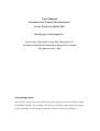
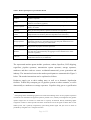
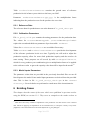
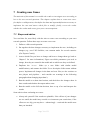
the natural gas trade flows in the model is explained in detail. Figure 1 shows an
overview of the – about 75 – countries and regions that are incorporated in the World
Gas Model (Egging et al., 2009a). For larger regions in the figure the numbers in
parentheses indicate the number of sub-regions in the model. For example the US
consists of six model nodes. A full list of nodes and regions is provided in Section 10
. The model covers 98% of the total production and consumption in 2005 according to
BP (2008).
EU (22)
Norway
Switzerland
Turkey
Canada (2)
Mexico
USA (6)
Russia (4)
Central
Asia (4)
MiddleEast (7)
Other
Asia (11)
Africa (10)
South
America (8)
Australia
Figure 1 Geographic scope of the WGM2
Energy markets have many different types of agents and many possible interactions
may occur among them. When formulating a model for an energy market many
modelling decisions must be made regarding the representation of the actors. The
following agents will be separately represented in the World Gas Model (WGM).
2
Source for the blank map: http://en.wikipedia.org/wiki/Wikipedia:Blank_maps
Page 5 of 52
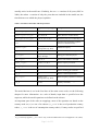
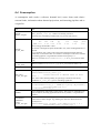
Table 1 Market participants represented in WGM
Agent
Role
Producer
Produces natural gas and supplies it to its trading arm and – if applicable –
domestic liquefiers
Trader
Buys gas from producers and sells it to marketers and storage operators (in
countries accessible by pipeline)
Pipeline Operator
Assigns pipeline capacity to traders who need to transport gas from one
country to another
Liquefier
Buys gas from the producer, liquefies it and sells it to regasifiers.
LNG shipping
vessels
Facilitate the overseas-transport of LNG from Liquefiers to Regasifiers.
(Represented in the model by distance-dependent costs and losses.)
Regasifier
Buys gas from liquefiers and sells it to the marketers and storage operators
Storage Operator
Buys gas in the low demand season from traders and – if applicable –
regasifiers and sells it to the market in the high and peak demand season to
take advantage of seasonal price differentials.
Transmission
System Operator
Responsible for pipeline network expansions3.
Marketer
Buys natural gas from traders, regasifiers and storage operators and distributes
it to end-users. (Represented by the aggregate inverse demand curve of the
consumer segments)
End users
The three consumption sectors: power generation, industry and
residential/commercial (see Marketer)
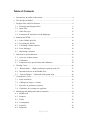
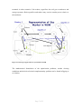
The represented market agents include: producers, traders, liquefiers, LNG shipping,
regasifiers, pipeline operators, transmission system operators, storage operators,
marketers and three end-use sectors: residential/commercial, power generation and
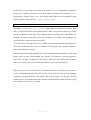
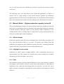
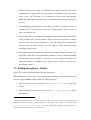
industry. The interactions between the market participants are summarized in Figure 2
below. The market interactions can be explained as follows:
Producers supply gas to their trading arms as well as to domestic liquefaction
facilities. Traders may transport gas via pipeline systems to other countries, or sell it
domestically to marketers or storage operators. Liquefiers ship gas to re-gasification
3
Anticipating further unbundling legislation we made the modeling choice to have pipeline expansion
investments not included in the pipeline operators problem. Also, initially we thought that the pipeline
operator might have an incentive to hold back in capacity investments thereby facilitating higher
congestion revenues in future periods. The latter would be the case if the agent would be able to exert
market power, but a perfectly competitively price-taking market agent will just invest as much as
predicted by: marginal costs = marginal revenues.
Page 6 of 52
terminals in other countries. Like traders, regasifiers also sell gas to marketers and
storage operators. Both regasifiers and traders may exercise market power relative to
the marketers.
Figure 2 Natural gas supply chain as represented in WGM
The mathematical formulation of the optimization problems, market clearing
conditions and the derived mixed complementarity problem can be found in Egging et
al. (2009a).
Page 7 of 52
3 Program Flow and File Structure
This chapter presents what happens in the WGM, in which order it does happen and
where you can find the files you may need to change in order to implement and run
cases. The folder structure and the program flow of the WGM are illustrated and
explained. There are three hierarchy levels within the WGM structure: the source
code and a number of auxiliary files; data and calibrations files; and case
specifications. You may define as many cases as you wish and there are few
restrictions on setting case specifications; you should, however, be careful about
changing data and calibration files and the code structure.
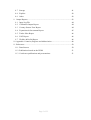
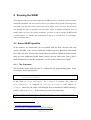
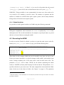
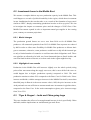
3.1 Hierarchy and Program Flow
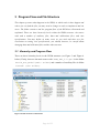
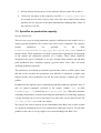
There are three hierarchy levels in the WGM structure (see Figure 3 and Figure 4
below). Firstly, there are the main source code ‘WGM_DET_2.0.gms’ in the folder
‘World_Gas_Model’ (Main Folder) and a number of auxiliary files in folder
‘shared’ (Aux Folder).
Figure 3 Folder structure of the WGM
Page 8 of 52
The auxiliary files are files independent of the data set and case you are running, such
as consistency checks, data processing and output report specification files. Other
files that show in Figure 3 in folder World_Gas_Model (ending in .gdx, gpr, log, lst,
lxi) are files produced by GAMS when running the model and can be ignored by the
reader.
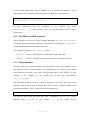
In folder ‘data’, you find one or more data sets of the following: ‘WGM’ or ‘RFF’
(the data sets for whole world); ‘aggregate’ (the data set used in the
INFRATRAIN) and ‘NOGER’ (this test data set contains only fake data for two
model nodes Norway and Germany and we use it in the manual to illustrate some
analysis methods for the model results). In each of the data set folders, you find a
folder named ‘calibref’ (short for calibration-reference). This is the second
hierarchy level of the WGM and it contains set declarations, reference values and data
set mappings – it can be thought of as the basic input data for this data set. Figure 4
illustrates the folder structure of the WGM.
Figure 4 Hierarchy and folder structure of the WGM
The third hierarchy structure consists of the cases, which are also located in the data
set folder. The ‘base’ case does not make any changes to the initial input data. We
Page 9 of 52
provide a number of other cases, which are described in more detail in Chapter 6 .
Chapter 7 explains how to define new cases according to your own specifications.
A user that wants to run the model has to define three main parameters. The data set
(<dataset>, e.g. WGM), the case (<case>, e.g. base) and the period
(<period>, e.g. 0520 for the period 2005-2020). These parameters can be found at
the top of the main source code ‘WGM_DET_2.0.gms’. The following describes
the program flow when the running the model.
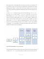
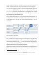
Figure 5 depicts the program flow of the WGM in relation to the hierarchy. The
model first declares all parameters and sets (Initialization). It then reads the input data
for the chosen data set. The input data are then modified according to the case
specifications.
Figure 5 Program flow of the WGM
Next, the input data are adjusted according to the specifications in the calibref files
and checked for consistency. If the model detects a problem (e.g., higher contract
obligation than production capacity in a country), the model run is aborted and an
explanation is written to a log file4. If no inconsistencies are detected, the WGM
continues with declaring the model variables and equations.
In some cases, it might be convenient to set certain variables to predefined values (for
instance, setting exports by a certain country to zero exogenously). This is done by
4
log_reading_input_<period>.txt in the folder /<case>/output/
Page 10 of 52
calling on a specific file in the case specifications: in_var_fx.gms. See section
4.1.3 for details.
Finally, GAMS casts the inputs into an equation system and calls the PATH5 solver to
attempt to find a solution. This can take several hours, depending on the computer and
the size of the problem, and the time and iteration limits specified. If the run is
successful (i.e. a solution is found, see chapter 4.3 ), GAMS creates a number of
output reports in the ‘/<case>/output/’-folder. These reports and the log files
are discussed in detail in Chapter 9 .
To summarize what GAMS does when you run the WGM:
1. Declare and define data sets and parameters
2. Adjust inputs according to case specifications
3. Calibrate input parameters
4. Consistency checks
5. Define variables and equations
6. Solve model
7. Produce output reports
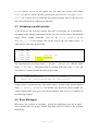
3.2 Input Files
The data input, calibration and case specification files are separated by player type. In
each of the input files, a header is inserted specifying the player type, all files specific
for that type, the file location and which file you are currently looking at. For
illustration, the header of the case file of the liquefier is shown in below:
$ONTEXT
inputs liquefiers
in_lng_data.gms
in_lng_calib.gms
in_lng_case.gms
in_lng_assign_check.gms
$OFFTEXT
5
sets, mappings, data tables
calibration tuning parameters
case specific adjustments
Data folder
Data folder
Case folder
assignments, input data checks
Aux folder
THIS FILE
GAMS comes with a free MCP solver MILES, however we always use the
proprietary PATH solver.
Page 11 of 52
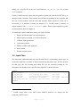
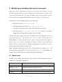
All files related to data input, data modification due to calibration and case
specification are listed in Table 2. The colour code indicates how sensitive this file is
to modifications, i.e. which files you may change without hesitation, and which files
you should be careful modifying.
Table 2 File types associated with data input and case specifications
File name
Folder
Player type
Description
in_case_global.gms
Case
-
General parameters of case
in_<type>_data
Data
all
Data set
in_<type>_calib
Data
all
Calibration to match base year
in_<type>_case
Case
all
Case specifications
in_<type>_ ships_contracts
Data
Regas
LNG shipping contracts6
in_<type>_ market_access
Data
Trad
Market access
in_<type>_ market_power
Data
Trad, Regas
Market power specifications
in_var_fx.gms
Case
-
Fixing variables exogenously
in_<type>_assign_check
Main
all
Check inputs
Green – these are the case specifications. You can simply create a new case by
duplicating the ‘base’-folder, rename the new folder (use a descriptive folder name
without spaces) and change any parameters to describe the case you want to run.
Yellow – these are input data. If you change any of these, it might be necessary to
recalibrate the model, which takes quite some time and skill. Before making any
changes to these files, ask yourself why it does not suffice to make this change in one
case only. Most users will not change these files, but will specify new cases only.
However if you need to change these, Chapter 8 provided details on how and what.
Orange – these are check files to ensure that there is no contradiction in the input data,
such as checks to ensure that there no producer has higher LNG contract obligations
than production capacity or every producer has a trader to sell to. If the model
encounters any problems, it will abort. Check the log-file to see where the problem
6
Adding or changing contractual values upward may cause production or liquefaction capacities to be
not sufficient anymore. The model will produce an error message if that is the case, however the user
may want to verify her-/himself.
Page 12 of 52
lies. Do not change anything in these files unless you are sure you understand the
code. Make a backup anyway, just in case.
Instructions on how to create new cases are given in Chapter 7 .
3.3 Other file types
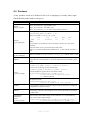
It is beyond the scope of this manual to describe all file types and their role in detail.
An overview is given in Table 3. As mentioned above, when modifying these files,
please be careful about what you do, keep a backup of the original file and test the
new file (for instance, by comparing model results before and after the change on a
small data set such as NOGER) before you interpret data from the modified model on a
large data set.
Table 3 Other input file types
Include files
all_<?>.gms
These files list other files to be included in the
model.
Output specifications
out_<?>.gms
These files define the data written in the output
reports. The output reports generated at the end
of a model run have the same name as the
output report specification files.
Declaration
declare_<?>.gms
Declaring sets and parameters
3.4 Parameters & Variables, Sets & Mappings
Variable and parameter names in the GAMS code follow the mathematical
formulation of the KKTs in Egging et al. (2009a) as closely as possible. Player sets
are indicated by the first letter of the player type (P for the set of producers, L for the
set of liquefiers, etc.). Elements of each set are prefixed by these first letters
(‘P_ALG’ is the producer in Algeria, ‘L_ALG’ is the liquefier in Algeria).
An overview of variables in the WGM and their interpretation is listed in Table 4; an
extensive list is given in the main source code ‘WGM_DET_2.0.gms’.
To facilitate the reusability of data input files as well as the definition of cases for
some sets, super and sub sets are defined where appropriate. For instance, PP is the
super set of all producers that can exist in the model; P is a subset of producers
Page 13 of 52
actually active in the model run.7 Similarly, the set YYY consists of all years (2005 to
2040), the subset Y consists of only the years that are included in the model run, the
time horizon over which the players optimize.
Table 4 Variables in the model and interpretation
Variable name
Applicable Player Types
Interpretation
Sales<type>_tot
A (arc), L, P
Total sales of player
Sales<type>to<type>
R, S, M; S, M
Sales (Decision variable Seller)
Buy<type>from<type>
L, R, S, T; P, L, R, T
Purchases (Decision variable Buyer)
Flow
T
Amount of gas shipped by pipeline
(Decision variable Trader)
CapNew<type>
L, R, Pipe,
Storage (Extr, Inj, WG)
Additional capacity
pi_W
Marketer
Wholesale (final demand) price
pi_<type>
L, P, RS (to Storage),
TS (to Storage)
Selling price between players
phi_<type>
L, R, S, T
Dual to mass-balance constraint
alpha_<type>
A (arc), L, P, R, S
Dual to capacity constraint
beta_<type>
P, S (Extr)
Dual to horizon constraint
gamma_S
S
Dual to working gas constraint
eps_R
R
Dual to contractual purchases
rho_<type>
A (arc), L, R,
Storage (Extr, Inj, WG)
Dual of capacity expansion constraint
tau_A
A (arc)
Congestion fee (dual to pipeline
capacity constraint)
The model horizon is set in the first lines of the main source code; see the following
chapter for more information. As a rule of thumb, input data is specified over the
supersets, while the model equations are defined on the subsets.
An important part of the code are mappings; most of the equations are based on the
country node set (n) or one of its subsets (n_prod is the set of production country
nodes, n_cons is the set of consumption country nodes). Country nodes are prefixed
7
E.g., a backstop supplier P_SUP is active only in the Post Bali Planet case in Huppmann et al. (2009).
Page 14 of 52
by the letter N; the country node Algeria is named ‘N_ALG’. Mappings tie together a
player (e.g. a producer) and the country node where it operates. For example, P_ALG,
the producer ‘Algeria’ and N_ALG. the country node Algeria are tied together by the
following line of code (in file ‘in_prod_data.gms’):
NdOfProd(‘P_ALG’,’N_ALG’) = 1;
Similarly, ProdNdOfTrad(t,n_prod) maps trader t to production node n_prod
and is used in the model when defining that a trader can purchase natural gas at the
specific production nodes only. This mapping structure grants a lot of flexibility: for
example, it allows tying more than one producer to a trader. All mappings are
specified in the respective player type files.
To avoid erroneous inputs, there are a number of consistency checks implemented in
the code, called before the solver is executed. For example, any producer cannot be
tied to more than one country.
Naming conventions and mappings have been implemented accordingly for all other
player types as well. When adding new players (for instance, a storage operator),
make sure you add a mapping for this player; otherwise, the model does not know
where it is located. (See section 8 for more details on how to add a player).
When you first see the WGM it may seem that the model set-up and file structure is
overly complicated. Realise that the current set-up with all case specific changes
completely separate from the data allows that several people can develop and run
various sets of cases at the same time, and can easily integrate all the work by coping
some folders from one PC to another.
Page 15 of 52
4 Running the WGM
This chapter first presents some important GAMS specifics, which may go beyond the
standard commands you learn when you first get to know the program. Knowing these
will make your life much easier when you start to define your own cases. We then take
you through the steps to actually run the model: where to modify commands, how to
modify them, etc. Once the model terminates, you have to check whether GAMS found
a valid solution, or whether the termination is due to a critical error or reaching a
time or iteration limit.
4.1 Some GAMS specifics
In this manual, we assume that you are familiar with the basic structure and code
syntax of GAMS. If not, please consult the GAMS tutorial by Richard E. Rosenthal8
first. Once you have mastered the simple transport problem explained in this tutorial,
there are some additional GAMS features which you may find useful. This is only a
short introduction; for full documentation, we refer to the GAMS Users Guide9.
4.1.1 The $ operator
The $ operator works much like the ‘if’-command in any programming syntax. Look,
for instance, at the following line:
Current_Parameter(element)$(Help_Parameter(element)>0) =
New_Parameter(element) ;
If the value of Help_Parameter for element is positive, the value of
New_Parameter
is assigned to Current_Parameter with respect to
element. Otherwise, the value is not changed. Keep in mind that GAMS considers a
positive value to be TRUE, so the following would work identically:
Current_Parameter(element)$Help_Parameter(element) = New_Parameter(element);
8
www.gams.com/dd/docs/gams/Tutorial.pdf
9
http://www.gams.com/dd/docs/bigdocs/GAMSUsersGuide.pdf
Page 16 of 52
A very useful application of the $ operator is as a selection mechanism, e.g. for
summing the sales volumes of only the producers mapped to a specific node n:
…
sum(p$NdOfProd(p,n), SalesP_tot(p,d,y))
…
In
this
summation
only
the
producers
p
are
selected
for
which
NdOfProd(p,n_prod)has a positive value (i.e. only the producer which is active
at that node).
4.1.2 The ORD and CARD operators
These operators are used to count elements belonging to a set. ORD(element)
returns the place at which the element occurs in the set it belongs to. CARD(set)
returns the total number of elements in this set.
For example if we have a SET X/A,B,C/ then:
ORD('B')
returns 2 (B being the second element in the set), and
CARD(X)
returns 3 (because of the presence of three elements in the set).
4.1.3 Fixing Variables
You may want to set certain variables to specific numeric values. For instance, we use
this approach in the ‘Eastern Promises’-case (Huppmann et al., 2009) to set exports
from Russia to zero after 2010. Due to the program flow in the WGM, it is only
possible to fix variables in one certain file in the case specifications
(in_var_fx.gms).
The following example from the ‘Eastern Promises’ case fixes the sales of the
Russian trader to any country in Europe after 2010 to zero, i.e. Russia cannot sell to
European consumers. This is achieved by the following line:
SalesTtoM.fx(‘T_RUS’,n,d,yyy)$(ORD(yyy)>2 AND InSRegion(n,’EUR’)) = 0;
This line of code means the following: sales to marketers [SalesTtoM] by the
Russian
trader
[T_RUS]
in
any
country
Page 17 of 52
[n]
in
the
region
Europe
[InSRegion(n,’EUR’)] is fixed [.fx] to zero for all periods after the second
[ORD(yyy)>2](since 2010 is the second element in the set of years ‘yyy’.10).
WARNING: Fixing variables is not recommended for most users. One needs to be
very careful to fix variables to specific values. The number of equations and the
number of variables in an MCP must equal (‘square system’) and in many situations
fixing values will result in a not square system.
4.1.4 Global Variables
It is possible to define global variables in GAMS using the following command:
$SETGLOBAL name "value"
During the compilation, each occurrence of %name% is replaced by value in the
subsequent code. We use this mechanism, for example, to specify the data set, period
and case to be used when executing the model.
4.2 Executing the WGM
In order to run the World Gas Model, you have to open the main source code file,
namely WGM_DET_2_0.gms. At the very top, you find the following lines:
******************************************************************
*
MAIN SETTINGS
******************************************************************
$SETGLOBAL dataset "WGM"
$SETGLOBAL case
"base"
$SETGLOBAL period
"0540"
These three are the settings, which you need to modify every time you run a case.
Unless you want to introduce very specific changes in the model, you actually do not
need to change anything else in the main source code but these three lines. The
parameter dataset can be either ‘WGM’ for the dataset containing the whole
world, or ‘NOGER’ (Norway and Germany) for the test data set. The parameter case
specifies which case you want to run. The value assigned here must match the folder
name of the case in the data set folder. (See Figure 3 at page 8.) The parameter
10
Note that subset y is not considered to be an ordered set, therefore the super set needs to be used in
the ORD() statement
Page 18 of 52
period allows you to run the model over the total time horizon (2005-2040;
‘0540’) or only for shorter periods (reducing the period in five year steps: ‘0535’,
‘0530’, etc.). Please keep in mind that one should maintain 2005 as the start year
since the model has been calibrated on that basis.
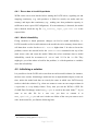
4.3 Validating a model solution
A WGM run for the full time horizon may take several hours on a standard PC;
depending on the changes implemented in the case, the run time may be substantially
longer. When GAMS terminates, look for the solve
summary in the
WGM_DET_2_0.lst-file (double click on the word in the left window pane.). A
valid solution looks like the following:
S O L V E
MODEL
TYPE
S U M M A R Y
WGM
MCP
SOLVER PATH
**** SOLVER STATUS
FROM LINE
1 NORMAL COMPLETION
**** MODEL STATUS
1 OPTIMAL
5282
The keywords here are solver status ‘1 NORMAL COMPLETION’ and the model
status: ‘1 OPTIMAL’. The model status is repeated at the end of the lst-file, and
one sentence is written whether the run was successful.
----
5286 Model Status:
MODEL WGM.ModelStat
----
5288 If this is displayed the model did solve correctly.
=
1.000
Output reports are generated only if the model status is at least locally optimal (Model
Status: 2 Locally Optimal). You should now proceed to check whether the
results actually make sense given your model changes; how to do so is explained in
the following chapters.
4.4 Error Messages
Most errors you are likely to encounter – apart from compilation errors due to typos –
can be divided into two groups: invalid input data, and errors that are due to model
infeasibility.
Page 19 of 52
4.4.1 Errors due to invalid input data
WGM carries out several checks before starting the PATH solver, regarding set and
mapping consistency (e.g. each producer is linked to exactly one trader and one
country) and input data consistency (e.g., making sure that production capacity is
sufficient to meet export LNG obligations). If an inconsistency is detected, the model
run is aborted; check the log file log_reading_input_<period>.txt in the
output folder.
4.4.2 Model infeasibility
Fixing variables or harsh parameter changes can lead to model infeasibility, i.e.
PATH is unable to find a valid solution to the model; the solve summary shown above
will then show a value for the Model Status higher than 2. In order to locate the
problem, remove the asterisk before the $OFFLISTING command at the top of the
main source code and rerun the model. When the solver terminates due to model
infeasibility, search for occurrences of ‘INFES’ and ‘****’in the lst-file. They
might give you a hint where to look for the problem, i.e. which equations or variables
cause the infeasibility.
4.5 Initialising a solution
It is possible to let the PATH solver start from an earlier model solution (for instance,
the base case results). Initialising a model run has an unpredictable impact on the run
time, unless the model and data are exactly the same in which case PATH merely
needs to check the solution. E.g., when one wants to create an extra output column in
a report this is a very handy feature. Every time you run the WGM, a GDX file
(GAMS Data Exchange) named WGM_p.gdx is saved in the main folder11. If you
want
to
use
this
file
for
a
case
run,
you
have
to
rename
it
to
WGM_<period>_p.gdx and save it in the case folder of the case you want to use it
with. In the main file, you find the following lines:
11
This is done by setting option Savepoint=1;
Page 20 of 52
****************************************************************************
****
DEVELOPER'S AND TEST SETTINGS
****************************************************************************
*Unmark if want to initialize the solution
$SETGLOBAL setinitsoln "*"
*Unmark debug if want more info in listing file
$SETGLOBAL debug "*"
Deleting the asterisk in setinitsoln “*” lets GAMS look for a GDX file in the
case folder – if it doesn’t find one, the model run will abort or just start from scratch!
In order to successfully initialise a case run, the number of variables in the gdx file
and the case must match; i.e., adding a player or a pipeline means that you cannot
initialise from a previous gdx file. In addition, the solution of the gdx file must lie in
the feasible region of the case run; i.e., restricting a value to a level lower than the
solution will return an error message (e.g. a lower value for production capacity than
the actual production volume in the solution saved in the gdx file).
Page 21 of 52
5 Data sources and calibration
This chapter provides an overview of the data on which the WGM is based: sources
from which the data was collected, and how we proceeded to make data from different
sources consistent.
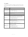
Table 5 Data source overview
12
Data category
Data types
Sources
Producer
Production cost parameters, capacities,
development of production capacities and
costs
Natural Gas Information, (IEA 2007);
Oostvoorn et al (2003); OME 2005; Stern
2006. Statistical Review of World Energy (BP
2008), WEO 2006, 2008; EC Trends in
European Transport and Energy (2005, 2007)
Trader
Market power
Model team choice, with some adjustments
during calibration
Pipeline Operator
Distance and type of pipelines
(onshore/offshore/ long-distance) pipeline
fees
World Energy Outlook (IEA 2008); GTE
(2005); Black Sea Energy Survey, (IEA 2000);
Statistical Review of World Energy. (BP,
2007); EIA Website; South American Gas
Daring to tap the Bounty, (IEA 2003).
Liquefier
Trade flows, capacity, costs, losses,
conversion factor, LNG contracts, projects
under construction/planned, investment
costs
Natural Gas Information, (IEA 2007);
Statistical Review of World Energy. (BP,
2007); The Global Liquefied Natural Gas
Market, (EIA 2003); LNG Fact Sheets, (BG
LNG Services 2005); LNG Map, (GLE 2005).
LNG shipping
vessels
costs and loss rates, distances
Colton Company, www.distances.com
Regasifier
see Liquefier
see Liquefier
Storage Operator
Working gas capacity, extraction and
injection rate, costs, losses
Natural Gas Information, (IEA 2007);
Oostvoorn et al. (2003) OME 2005; Natural
Gas in Western Europe, (Eurogas 1998);
Flexibility in Natural Gas, (IEA 2002).
Transmission
System Operator
Projects under construction/planned,
investment costs
Personal communication (ICF Consulting,
2008); Developing China's Natural Gas
Market, (IEA 2002); World Energy Outlook,
(IEA 2005, 2008).
Marketer
see End User
End users
Energy Statistics Manual, (IEA 2005);
Statistical Review of World Energy. (BP,
2007); EIA Website; Annual Report 2005,
(GasTerra 2006). WEO 2006, 2008; EC Trends
in European Transport and Energy (2005,
2007)
12
Consumption by sector, price-elasticity,
development of consumption by country
For periodic publications, only the most recent version used is stated; if these did not contain all the
needed inputs earlier versions have been used as well.
Page 22 of 52
5.1 Overview of data sources
The sources from which we collected the input data for the WGM are listed in Table
5. See Egging et al. (2009a) for further details.
5.2 Calibration
At some point when the model has been thoroughly checked and tested on a small
data set we trust that the implemented functionality is as desired. The next step is to
compile all the collected data in an appropriate format for GAMS to use. When one
runs the model on the full data set, typically the outcomes are not as desired. Model
outcomes for some countries’ production are too high, for others too low. Outcomes
for consumption and prices deviate from observed, acceptable or required outcomes.
Et cetera. Some reasons for the deviations between model outcomes and desired
outcomes are: inconsistencies in the data, unavailability or unreliability of the data
sources or the necessary assumptions and simplifications and aggregations when
specifying the model. An important step in model development is calibration, loosely
speaking: the tuning of the input parameters to facilitate that model outcomes (for a
reference case) are equal to (or close enough) to desired outcomes.
The person who calibrates the model has several decisions to make. What are the
desired outcomes? Which outcomes are most important to get close? What flexibility
do I allow myself in changing input parameters? What input parameters should I keep
as collected, and what are the ones that allow larger adjustments?
Typically we prefer to adjust the most unreliable data and the parameters that are
completely analyst-determined. Also, if the focus of the analysis is on some part of
the world, e.g. Europe, then the model outcomes for other continents need not be as
carefully and closely tuned as for Europe. E.g. for Europe we may want to have
production and consumption in all countries within 1% of the reference values; but for
countries at other continents we may say within 3%, as long as the whole continent on
an aggregate level is within 2%.
The first step should be to define the reference values for the desired aggregation
levels. It is highly preferable to find as few data sources as possible that cover as
much as possible of the model outcomes. Sometimes the data sources used when
Page 23 of 52
collecting the input data sets are also good sources for the reference data, but not
always. E.g. if we use IEA data as input for sector consumption levels in 2005, it
makes sense to use those same data as reference values.
For every data category the collected input data are specified in files with names
‘in_<type>_data’. The adjustments made during calibration to have the Base
Case
outcomes
match
the
reference
values
are
specified
in
files:
in_<type>_calib.
Most data specifications and adjustments are straight-forward adjustments of costs
and capacity values. For example for the liquefiers the file ‘in_lng_data.gms’ contains
a table with capacities (cap), loss rates (loss) and costs (lin):
Table LiqData(l,*)
cap
loss
L_AFR
182.6
0.12
L_ASP
264.1
0.12
lin
30
30
…..
In the file in_lng_calib.gms, the collected values for costs are overridden with the
following statement:
LiqData(l,'lin') = LiqData(l,'lin') + 25 ;
Which means that all costs (in $/kcm) are increased by 25 units, from 30 to 55.
Most other data inputs and adjustments have a similar form as for the liquefier. Due to
the complicated functional form of the production costs curve, we give some more
background for the specification of the input parameters of the production costs.
5.3 Production costs specification and calibration
The basic input data for the producer are in file: in_prod_data.gms. This file
contains a number of tables and some separate parameters.
Table ProdData contains production cost function parameters and capacities.
Dependent on the data set, the production rate is either set equal to the collected value
for the production capacity (WGM full data set) or to the reference outcomes for
Page 24 of 52
production (aggregate data set)13. The production horizon represents the gas reserves,
but since we have no reliable reserves data these values are set to a high value to not
be limiting14. The other parameters are used for the ‘Golombek’ production cost
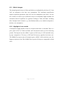
1
Q−q
function. (Golombek et al. 1995.) C ( q ) = (α − γ )q + β q 2 − γ ( Q − q ) ln
For
2
Q
Q−q
. In
which the marginal supply cost curve looks like: C ' (q ) = α + β q + γ ln
Q
here, Q is the production capacity, α > 0 is the minimum per unit cost, β ≥ 0 the per
unit linearly increasing cost term, and γ ≤ 0 a term that induces high marginal costs
when production is close to full capacity. In Table ProdData the first parameter is
α, the second parameter is the maximum per unit supply costs at full capacity when
not considering the logarithmic term (mmQ, see CostProdMaxMargQuadr in the
calibration file). The third parameter is the maximum per unit cost at 99.9% of
capacity (since ln(0) is not defined.) (mmG, see CostProdMaxMargGolombek in
the calibration file).
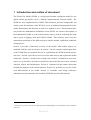
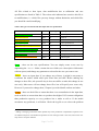
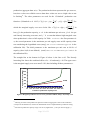
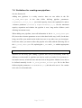
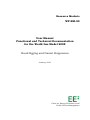
The straight line at the bottom in Figure 6 below is the line α=10. The linearly
increasing line shows the combined effect of α = 10 and mmQ = 40. The upper curve
is the marginal supply cost curve mmG=120, thus including all three parameters15.
mmG
marginal prod costs ($/kcm)
$120
$100
$80
$60
mmQ
$40
$20
α
$0
0.0 10.0 20.0 30.0 40.0 50.0 59.9 69.9 79.9 89.9 99.9
Fraction of production capacity used
Figure 6 Marginal production cost curve for parameters α=10, mmQ = 40, mmQ = 120
13
Allowing for slack in the production capacities in data set aggregate is done in the calibration.
14
Except for the full data set, wherein for Netherlands we have implemented a production ceiling.
15
Note that at production capacity usage over 99.9%, higher than γ costs per unit will apply (!)
Page 25 of 52
Table ProductionGrowthFactors contains the growth rates of reference
production levels in future years relative to the base year 2005.
Parameter
ProdCostGrowthFactor(pp,yyy) is the multiplication factor
indicating how the production costs for the producer rise over time.
5.3.1 Reference Data
The reference data for production are set at the bottom of in_prod_data.gms
5.3.2 Calibration Parameters
File in_prod_calib.gms contains the tuning parameters for the production data.
The values for CostProdMaxMargQuadr ,CostProdMaxMargGolombek
replace the second and third cost parameter of previous table ProdData.
Values for ProdCostGrowthFactor are overridden if necessary.
Tables ProdData and ProductionGrowthFactors provide the developments
of the reference production levels over time. Typically one will need to adjust the
production capacity, allow for some slack production capacity and also need to do
some tuning. These purposes are all served by table ProdCapCalibFactor,
which for every producer-year combination gives a multiplication factor to be applied
to the reference value to get to the capacity value that will be input for the model.16
5.3.3 Model Inputs Parameters
The parameter values that are provided in the previously described files are not all
literal input to the model. Some model input parameters are derived from the provided
data. This is done in file in_prod_assign_check.gms in the <shared
directory>. Several checks are performed to catch most of the inconsistencies.
6 Existing Cases
This chapter describes some of the cases which were published in previous articles
using the WGM, see section 11.3 . They serve as examples to the reader on how to
16
There have been many calibration adjustments to the production cost data relative to the collected
data. Instead of applying all adjustments in the calibration file, in retrospect contrary to my better
judgement, some of these data have also been adjusted in in_prod_data.gms
Page 26 of 52
turn a research question into a WGM case, and how to quickly check whether results
make sense.
The following cases were done based on the WGM and published in a number of
articles. Due to slight changes to the model and the updated and differently
aggregated data sets after the previous publications it is not guaranteed that rerunning
these cases with the current model version would give the same numerical outcomes.
6.1 ‘Barnett Shale’ – Higher production capacity in the US
The recent technological advances in unconventional natural gas production in the US
have led to a reassessment of the development of the natural gas production capacities
in North America, with great impact on the expected import dependency in the
coming decades. Since no reliable data on actual size of reserves and production cost
exist yet, we make rather crude assumptions.
6.1.1 Model changes
Production capacities from 2010 on are multiplied by 4 for the shale gas regions (US
East, Gulf and Rockies) and by 2 for other US regions and Canada. Note that
production cost depend on total production capacity; therefore, extending production
capacity will lead, ceteris paribus, to lower unit production costs.
6.1.2 Highlight of case results
Production in North America roughly doubles, while consumption increases by
approximately 20%. LNG imports are virtually non-existent, compared to an import
dependency of 40% in the Base Case in 2030.
6.1.3 Note
The production capacity increase implemented here is very steep and large; a gradual
rise might be more realistic. However, as the aim of this manual is to show how to
implement a case, rather than developing ideal cases ourselves, we leave it to you to
ponder on better assumptions regarding the actual production development in North
America.
Page 27 of 52
6.2 Investment freeze in the Middle East
We assume a complete halt on any new production capacity in the Middle East. This
could happen as a result of political instability in the region, which deters investment
in new installations for the next decades, or as a result of the formation of a gas cartel
similar to OPEC, sharply constraining production in order to drive up prices. We aim
to investigate the impact on consumer prices and the changes of LNG flows if the
Middle East cannot expand its role as important natural gas supplier in the coming
years, contrary to common projections.
6.2.1 Model changes
The production growth factors are set to zero from 2010 on for all Middle East
producers. All contracted quantities from 2015 for Middle East exporters are reduced
by half in order to allow more flexibility for Middle East producers to allocate their
gas to consumers; otherwise, some producers would have to ship all their natural gas
to only a limited number of countries or could not meet their obligations at all. Three
new pipeline are allowed to be built, two from Oman and Qatar to Saudi Arabia, and
one from Saudi Arabia to Kuwait, to see how trade in the region might develop.
6.2.2 Highlight of case results
Production in the Middle East still increases slightly over the whole period (rising
prices allow movement along the supply cost curve; this is not a shift of the curve as
would happen due to higher production capacity) compared to 2010. The total
production remains at about 50% compared to the Base Case for 2040 levels. Prices
increase worldwide, with the strongest increases in the Middle East itself (a more than
threefold jump in Kuwait is the most extreme value). Still, the price increases on the
Arab peninsula are not sufficient to warrant much more investment in pipelines there,
compared to the Base Case. In the main consumption regions, price increases range
from 3% to 25%.
6.3 ‘Tiger & Dragon’ – India and China going large
This case simulates the effects of a strong demand increase in Asia, specifically China
and India, and the implications on world natural gas trade flows.
Page 28 of 52
6.3.1 Model changes
The demand growth factors in China and India were multiplied by the factor 2.5 from
2015 on compared to the base case assumptions. The maximum regasification
capacity expansion parameters from 2015 on were multiplied by the factor 3 for the
two countries in order to give sufficient leeway to accommodate higher demand. All
maximum allowed expansions for pipelines leading to China and India, including
those through transit countries (e.g. Iran-Pakistan-India), were doubled compared to
the base case assumptions.
6.3.2 Highlight of case results
Consumption roughly doubles in the two countries until 2030, as intended. There is a
price spike in 2015 in China and India, until investments catch up in the following
periods. The imports into the ASPAC region are 288 bcm/y in LNG and 448 bcm/y
by pipe, compared to 170 bcm/y as LNG and 326 bcm/y by pipeline in the base case.
The Middle East exports most of its natural gas to ASPAC, while in the base case, the
biggest recipient are the USA; Middle East exports to Europe are comparable in both
cases.
Page 29 of 52
7 Creating new Cases
The main aim of this manual is to enable the reader to investigate cases according to
her or his own research questions. This chapter explains how to create new cases:
first define a valid question; then define the data and input modifications necessary to
implement the case and assess which files to modify; finally, screen the results
whether the results make sense given your case assumptions.
7.1 Steps and advice
You read thus far, most likely with the aim to create cases according to your own
research question. Follow these steps to create a new case:
1. Define a valid research question.
2. Put together the data changes necessary to implement the case, including set
changes (e.g., new LNG facilities, one common trader for several countries
(Gas Exports Cartel)).
3. Assess which files you have to change and how to change them (go back to
Chapter 3 for more information). Figure out which parameters you need to
change, how they are named in the model and on which sets they are defined.
4. Duplicate the ‘base’ folder (or a case folder with similar model
modifications), and rename the folder. Use a descriptive folder name without
spaces. Implement all changes in the data and case files (see the sections on
new players and pipelines – and consider our warnings in the following
paragraphs about changing input data!).
5. Run the model on a short time horizon, and check how the changes show in
these results and whether the output makes sense.
6. Run the model on the full time horizon, have a cup of tea and interpret the
results.
Some advice when evaluating new cases:
•
Always ask yourself if the results are plausible; if the effects of your changes
are too small, the model may override or circumvent your restrictions; if the
effects are too big, you may have – unknowingly – restricted the model more
than you intended.
Page 30 of 52
•
When evaluating case results, you should always ignore (and leave out of any
evaluation) the results of the last two periods. Investments need some future
years to pay off. Therefore, the investment decisions and, consequently,
production and supply decisions may be distorted in the last two periods of
any run.
•
Avoid changing any parameters for the base year 2005, since this will mess up
calibration. E.g., if you specify new players, let them only be active in 2010 or
later. (See Section 8.2 ).
•
It is usually much easier and more straightforward to look at the modifications
in the example cases provided than to figure out how to implement a change
from scratch. If you want to implement a case with similarities to another one
that has been specified already, you can copy the files and adjust them
according to your needs.
•
You might want to automate the evaluation of output reports, for instance by
importing results into Excel spreadsheet templates. Keep in mind that adding
new elements such as pipelines or players (e.g. a new liquefaction plant) will
affect the number of variables in the output reports and may mess up your
automation routine!
7.2 Adding new players - Outline
Please see section 8 for detailed specifics for each player.
When adding new players (e.g. a new regasification plant in a country which does not
have one in the standard setup), follow the following steps:17
1. Add the player to the respective set (declare_sets.gms in the data
folder)
2. Add a mapping for the player if necessary (in_<type>_data.gms in the
data folder)
17
Adding an additional plant to a node where this player type already exists is, from the model
perspective, merely a capacity expansion and not a new player; this change can be made in the
in_<type>_data.gms or in_<type>_case.gms respectively, depending on whether the new
capacity is relevant for all cases or just some cases.
Page 31 of 52
3. Provide all data for this player for the total time horizon (same file as above)
4. ‘Switch on’ the player in the respective case file (in_<type>_case.gms)
if you want it to be active only in some cases; this can be achieved by setting
capacity zero for all years in the input data and then changing these values in
the respective case file
7.3 Specifics on production capacity
See also Section 8.8 .
There are two ways in which production capacity is influenced in the model: one is a
capacity growth parameter, the second is the total reserve constraint. The capacity
growth
parameters
are
specified
in
the
table
ProductionGrowthFactors(pp,yyy) in in_prod_data.gms, located in
the data folder. These parameters are based on projections regarding the development
of the natural gas production potential of a country. These values implicitly
incorporate the reserve constraint, as we have assumed that countries beyond their
peak production have declining capacity (growth values lower than one mean
declining production capacity).
The parameters are denoted as cumulative growth rates relative to 2005 values. Note
that due to the way how the production cost function is calculated, a higher total
capacity means lower production cost for the same amount of natural gas, ceteris
paribus.
In addition to the implicit reserve constraint through the production capacities, there is
also an explicit parameter provided in the model: column ‘hor’ in table
ProdData(pp,*,*), located also in in_prod_data.gms. When this constraint
is binding, the producers consider inter-temporal optimization a la Hotelling, applying
a yearly discount rate of 10% in the Base Case (this value can be altered in the file
in_case_global.gms in the case folder).
We only use the reserve horizon for the Netherlands in the Base Case to take account
of a political commitment not to over-exploit their natural gas reserves. For all other
producers, this value is set very high so as to not be binding in the Base Case.
Page 32 of 52
7.4 Guidelines for creating new pipelines
See also Section 8.8
Adding new pipelines is a tricky exercise: there are two tables in the file
in_trad_data.gms
in
the
data
folder
defining
pipeline
parameters:
PipeData(n_out,n_in,*) sets initial capacity, losses, the regulated fee and an
‘existence parameter’ (‘exists’); PipeInvParms(*,*,*) sets the maximum
capacity expansion and whether the pipeline is new, long and/or offshore (each
affecting investment costs).
When adding new pipelines, insert all information in the in in_trad_data.gms
file, but set the existence parameter to zero in the data. In this way, it will, for the time
being, not affect your model results in the base case or any other case you investigate.
In the case where you want to allow this pipeline to be built, add the following line in
the in_trad_case.gms file, replacing the n_out and n_in with the appropriate
nodes:
PipeData(n_out,n_in,’exists’) = 1;
And now for the tricky part: adding a pipeline does not yet necessarily make any
difference to the model! A pipeline can only be used by a trader if it is present (i.e.
has market access) at both the start and end node of the pipeline. Market access has to
be defined manually in the in_trad_market_access.gms file in the Data
folder using the parameter TransmAtNd(tt,n); this has to be set to 1 for a trader
to be active at a demand node.
Page 33 of 52
8 Modifying and adding data and set elements
Many cases can be implemented just using a set of case files. However, in some
situations the model data set needs to be adjusted or extended with extra players. This
section gives directions how to do that. In addition, this section provides a step by
step tutorial for expanding the WGM data set with new players or infrastructure.
In general, the steps for adding a player are the following:
•
Add player to set in declare_sets.gms
•
Add mapping and player data to in_<type>_data.gms
(for trader and regasifier resp. 2 and 1 other files need to be edited).
•
Add player data to in_<type>_case.gms. It is advised to not make
changes that would change the outputs for the year 2005.
Warning: the name country_node can be confusing. Due to the aggregation levels in
some of the data sets – e.g. the data set aggregate that we have used in the
INFRATRAIN – for several regions there is only one country node in the region. In
data set aggregate the two exceptions are Europe, with five country nodes, and
Russia, with two country nodes. To make the aggregation level explicit we can use
the term model node instead of country node.
Make a complete backup before you start. Then duplicate the folder base, and
rename the copy appropriately. We refer to the copy as <case>. After making your
changes, check that the base case still produces the same outcomes.
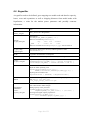
8.1 Model node
A model node (country node) needs a region, and also other characteristics such as
production, consumption, pipelines etc.
Files
Edits
calibref\ declare_sets.gms
add N_NEW to the set N "all nodes"
calibref\
in_assign_global.gms
In bottom part where the regions are specified:
InSRegion('N_NEW',<region>) = 1 ;
OTHER
Need to add production, consumption or infrastructure information
WARNING
Not adding more information will result in an error message and abort
Page 34 of 52
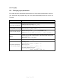
8.2 Producer
A new producer needs to be defined in two sets, a mapping to a country node, input
data definitions and a trader to sell gas to
Files
Edits
calibref\
declare_sets.gms
add P_NEW to the set P "all producers" and
add N_NEW to the set N "all nodes", and
add N_NEW to the set N_prod "nodes of producing countries"
calibref\
in_prod_data.gms
Add mapping
NdOfProd("P_NEW","N_NEW") = 1 ;
Add a row to table ProdData for P_NEW
*
rate
hor
lin
mmQ
mmG
P_NEW
0.1
10000000
20
45
70
HINT:
By including a low production rate the results for the base case will not be
disturbed.
look at the other rows to get an idea about valid values
Add a row to Table ProductionGrowthFactors for P_NEW with the all values =
1.00
calibref\
in_prod_calib.gms
Add row to Table ProdCapCalibFactor(pp,yyy), with all values = 1.00
CHECK
run the base case (for a short period, e.g. 0520, otherwise you will be waiting
long) and look in the listing file or one of the output files for proof that N_NEW
exists
<case>\
in_prod_case.gms
Override the production rate
ProdData(‘P_NEW’,’rate’)= <value in mcm/d> ;
Prevent an error message for inconsistent data:
ProdRef('N_NEW')=ProdData('P_NEW','rate') ;
Override production growth factors (but not for 2005)
ProductionGrowthFactors(‘P_NEW’,yyy) =
<value relative to the base year> ;
i.e., 1 means no growth
Advanced overrides:
ProdCostGrowthFactor(pp,yyy) =
<value for production cost growth> ;
OTHER
A new producer needs to get a trader assigned, and also domestic consumption
or liquefaction or pipeline outlets
CHECK
run the <case> case (for a short period, e.g. 0520, otherwise you will be
waiting long) and look in the listing file or one of the output files for proof that
N_NEW exists
CHANGING
EXISTING
<case>\
in_prod_case.gms.
There can have been made changes in the calibration. It is recommended to
refer to data itself to make changes:
ProductionGrowthFactors(‘P_XYZ’,yyy)$(ORD(yyy)>2) =
2*ProductionGrowthFactors(‘P_XYZ’,yyy) ;
Page 35 of 52
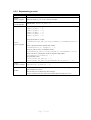
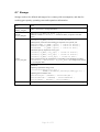
8.3 Trader
8.3.1 Changing input parameters
For traders the most important characteristics are from which producers they can buy
gas, what nodes and pipelines they can access, and what market power the exercise at
all nodes.
Files
Edits
calibref\ declare_sets.gms
add T_NEW to the set T
calibref\ in_trad_data.gms
Affiliate trader with producer <n_prod>
ProdNdOfTrad("T_NEW",<n_prod>) = 1 ;
calibref\
in_trad_market_access.gms
Define market access at <node>
TransmAtNd('T_NEW,<node>) = 1;
<case>\ in_trad_case.gms
Define market power at <n_cons> (only needed if > 0)
CournotPower('T_NEW',<n_cons>) = <value between 0
and 1>;
CHECK
run the <case> case (for a short period, e.g. 0520, otherwise you will be
waiting long) and look in the listing file or one of the output files for proof
that N_NEW exists,
then run the <base> case (same)
OTHER
May need to define new pipelines
CHANGING EXISTING
<case>\ in_trad_case.gms.
Granting access
TransmAtNd('T_XYZ','N_ABC')= 1;
Removing access
TransmAtNd('T_XYZ','N_ABC')= 0;
Overriding market power value
CournotPower('T_XYZ', 'N_ABC')=
<value between 0 and 1>;
Page 36 of 52
8.3.2 Representing a cartel
Files
Edits
calibref\
declare_sets.gms
add a new trader T_GEC to set T, the set of traders
calibref\
in_trad_data.gms
add statement: InGec('T_GEC')=1;
InGec('T_GEC')
InGEC('T_RUS')
InGEC('T_AFR')
InGEC('T_MEA')
InGEC('T_SAM')
InGEC('T_CAS')
<case> \
in_trad_case.gms
=
=
=
=
=
=
0;
1;
1;
1;
1;
1;
Assign prod nodes to T_GEC
ProdNdOfTrad("T_GEC",n)$sum(t$InGEC(t),ProdNdOfTrad(t,n))
= 1;
Remove prod nodes from separate GEC traders
ProdNdOfTrad(t,n) $InGEC(t) = 0 ;
Assign T_GEC access to consumption nodes
TransmAtNd("T_GEC",n)$sum(t$InGEC(t),TransmAtNd(t,n))=1;
Remove access to consumption nodes for separate GEC traders
TransmAtNd(t,n)$InGEC(t) = 0 ;
Assign market power
CournotPower("T_GEC",n) = 1;
CournotPower("T_GEC",n)$ProdNdOfTrad("T_GEC",n) = 0;
<case>\
in_regas_case.gms
RegasData(r,'cournot') = 1;
NOTES
Due to different LNG and pipeline streams the above is merely a rough
approximation of a cartel.
Also the base year is affected by these changes.
In cartel countries both the cartel trader and the domestic trader are active.
Page 37 of 52
8.4 Consumption
A consumption node needs a reference demand level, sector shares and relative
seasonal loads, information about demand projections, and incoming pipelines and or
a regasifier
Files
Edits
calibref\
declare_sets.gms
if the node N_NEW pre-exists:
add N_NEW to N_cons (N) "nodes of consuming countries"
otherwise start with adding a model node (see previous sub section)
calibref\
in_cons_data
Add a row to Table ConsData(n,*)
*
ref
res
ind
pg
low
high
peak
N_NEW 0.03
0.33 0.33 0.34
1.00
1.00
1.00
res+ind+pg should add to 1.000
183*low+120*high+62*peak should add to 365, some rounding difference is
allowed
For a completely new country node with positive demand without domestic
production, it is advised to take as a reference consumption value 0.03, and have
an incoming pipeline or regasification terminal with capacity 0.1
Add a row to Table DemGrowthFactors(*,*) for N_NEW, with all values
1.00
calibref\
in_cons_calib
add row to Table ConsCalib(n,yyy) for N_NEW, with all values 1.00
CHECK
run base case and check for proof that the consumption node exists
data\<case>\
in_cons_case.gms
Define projections for the demand
DemGrowthFactors(<n_cons>,y) =
<value relative to demand level in base
year> ;
Note: these values should probably be quite large to make the 0.03 bcm/y
included in in_cons_data grow to something significant.
Advanced:
PriceGrowthFactor(n,y) = POWER(1+<%yearly adjustment>,
YearStep*(ORD(yyy)-1))*
PriceGrowthFactor(n,y);
OTHER
a new consumption node needs a supply source. This can be (a combination of)
local production, incoming pipelines (and access by traders ) or regasification
facilities.
CHANGING
EXISTING
<case>\
in_cons_case.gms
There can have been made changes in the calibration. It is recommended to refer
to data itself to make changes. E.g doubling the reference demand from the
second year on:
DemGrowthFactors (‘N_XYZ’,yyy)$(ORD(yyy)>=2) = 2 *
DemGrowthFactors (‘N_XYZ’,yyy) ;
Page 38 of 52
8.5 Liquefier
A liquefier needs to be defined, get a mapping to a model node, data for capacity,
losses, costs and expansions as well as shipping distances from its model node to
regasifiers.
Files
Edits
calibref\ declare_sets.gms
add L_NEW to set L "Liquefiers"
calibref\ in_lng_data.gms
NdOfLiq("L_NEW","N_NEW") = 1;
Add a row to Table LiqData(l,*)
*
cap
loss
lin
L_NEW
0
0.12
30
Add a row to Table MaxNewLiqCaps(l,*) for L_NEW, all values 0
calibref\ in_regas_ships
_contracts.gms
add shipping distances for the newly added liquefier to
Table ShDistance(n,r)
NOTE
a liquefier needs a domestic producer
CHECK
do a base case run
<case>\
in_LNG_case.gms
It is not advised to add liquefaction capacity in the first year (2005):
LiqData(‘L_NEW’,’ cap’) = <value cap in mcm/d> ;
If desired one can add liquefaction capacity in the second year (2010) :
LiqAddCapsHelp('L_NEW','curr') =
<value cap in mcm/d> ;
Allowing liquefaction capacity expansions:
MaxNewLiqCaps(‘L_NEW’,yyy) = <value in bcm/y> ;
Advanced:
overriding operational liquefaction costs
LiqCostGrowthFactor(‘L_NEW’,yyy) =
POWER(1+PriceInfl,YearStep*(ORD(yyy)-1)) ;
overriding liquefaction expansions costs
LiqInvCostFx = (FACTOR) * LiqInvCostFx ;
CHANGING EXISTING
<case>\
in_LNG_case.gms
There can have been made changes in the calibration. It is recommended to
refer to data itself to make changes.
Adding capacity in the year 2010:
LiqAddCapsHelp('L_LNG,'curr')=
LiqAddCapsHelp('L_LNG,'curr')+(5/0.365) ;
Allowing 50% higher capacity expansions
MaxNewLiqCaps(‘L_NEW’,yyy) =
1.5*MaxNewLiqCaps(‘L_NEW’,yyy) ;
Page 39 of 52
8.6 Regasifier
A regasifier needs to be defined, get a mapping to a model node and data for capacity,
losses, costs and expansions as well as shipping distances from model nodes with
liquefaction, a value for the market power parameter and possibly contracts
information.
Files
Edits
calibref\
declare_sets.gms
add R_NEW to set R "Regasifiers"
calibref\
in_regas_data.gms
Add mapping
NdOfRegas("R_NEW","N_NEW") = 1 ;
Add a row to Table RegasData(r,*)
*
cap
loss lin
cournot
R_NEW
0
0.015 10
0.25
Add a row to Table MaxNewRegasCaps(r,yyy) with all values 0
calibref\
in_regas_ships
_contracts.gms
add shipping distances for the newly added regasifier to Table
ShDistance(n,r)
NOTE
a regasifier needs domestic consumption
CHECK
run base case and check for proof that the newly added regasifier exists
<case>\
in_regas_case.gms
RegasAddCapsHelp(‘R_NEW’,’curr’) = <value in mcm/d> ;
MaxNewRegasCaps(‘R_NEW’,yyy) = <value in mcm/d> ;
CournotRegas("R_NEW") = <value between 0 and 1> ;
Advanced:
Adjust the future operating costs
RegasCostGrowthFactor(rr,yyy) =
POWER(1+PriceInfl,YearStep*(ORD(yyy)-1)) ;
Adjusting the investment costs
RegasInvCostFx = (FACTOR) * RegasInvCostFx ;
HINTS
SEE: data\<our_data_set>\calibref\in_regas_data.gms
SEE: data\< our_data_set
>\in_regas_ships_contracts.gms
CHANGING
EXISTING
<case>\
in_LNG_case.gms
There can have been made changes in the calibration. It is recommended to
refer to data itself to make changes.
Adding capacity in the year 2010:
LiqAddCapsHelp('L_LNG,'curr') =
LiqAddCapsHelp('L_LNG,'curr') + (5/0.365) ;
Allowing 50% higher capacity expansions:
MaxNewLiqCaps(‘L_NEW’,yyy) =
1.5 * MaxNewLiqCaps(‘L_NEW’,yyy) ;
Page 40 of 52
8.7 Storage
Storage needs to be defined and mapped to a country with consumption, and data for
working gas capacity, operating costs and expansions information.
Files
Edits
calibref\
declare_sets.gms
Add S_NEW to set S "storage operators"
calibref\
in_stor_data.gms
NdOfStor("S_NEW","N_ASP") = 1 ;
Add row to Table StorData(s,*) with all 0 values, except for costs and
losses.
<case>\
in_stor_case.gms
StorData(‘S_NEW’,’work’) = <value in mcm> ;
Add injection, extraction and working gas capacities in a specific year
MaxInjectAdd ('S_NEW',<year>) = <value in mcm/d> ;
MaxExtractAdd('S_NEW',<year>) = <value in mcm/d> ;
WorkGasAdd
('S_NEW',<year>) = <value in mcm> ;
Allowable capacity expansions in any year:
StorData('S_NEW','inj_exp') = <value in mcm/d> ;
StorData('S_NEW','xtr_exp') = <value in mcm/d> ;
StorData('S_NEW','work_exp') = <value in mcm> ;
Note: storage will only be used if there is seasonality in the demand. See Table
ConsData(n,*) in calibref\ in_cons_data.gms and previous section
on consumption data.
Advanced:
Adjusting operational storage costs
StorCostGrowthFactor(s,yyy) =
POWER(1+PriceInfl,YearStep*(ORD(yyy)-1)) ;
Adjusting the investment costs
InvCostSInjFx = (FACTOR) * InvCostSInjFx ;
InvCostSExtrFx = (FACTOR) * InvCostSExtrFx ;
InvCostSWGFx = (FACTOR) * InvCostSWGFx ;
WARNING
Adding storage to a country without consumption will result in an error message
Page 41 of 52
8.8 Pipeline
Files
Edits
calibref\
in_trad_data.gms
Add a row to Table PipeData with all meaningful values but capacity 0
Add a row to Table PipeInvParms with meaningful values for the first
three columns (New, Long, Offshore) but all allowable expansions a value of
0
<case>\
in_trad_case.gms
Add allowable expansions
PipeInvParms(<n_out>,<n_in>,<year>) =
<value in mcm/d> ;
WARNING
Can a trader access both outward and the inward node?
CHECK
run a <case> case and a base case, note that capacity expansions often need
at least two more periods after the expansion year to become profitable.
8.9 Other
Files
Edits
<case>\
in_case_global.gms
discountrate
priceinfl
= 0.10 ;
= 0.0313 ;
Page 42 of 52
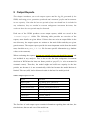
9 Output Reports
This chapter introduces you to the output reports and the log file generated by the
WGM, indicating prices, quantities produced and consumed, profits and investments
in new capacity. Note that the last two periods of any run should not be included in
any evaluation; they are needed to warrant endogenous investment decisions, but
results in these last two periods may be distorted.
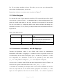
Each run of the WGM produces seven output reports, which are saved in the
‘<case>/output’ folder. The following table provides an overview of the
reports; more details are given below. If there does not exist an output folder in the
case directory, the output reports are written to the main folder and they are given
generic names. The output reports provide the most important results from the model
runs; check the WGM_DET_2.0.lst file for more specific information (e.g. shadow
values on investments).
When evaluating the reports, the last two periods of any run should be ignored and
not included in any analysis. This is due to the fact that endogenous investment
decisions in WGM need at least one future period to ‘pay off’ (i.e. to be warranted in
economic terms). Therefore, the model might not build new capacity in the last
periods, not because it is not economically viable but because the model horizon is
limited. This can (will) lead to distorted results in the last few model periods.
Table 6 Output report overview
Report
File Name
Input Log File
log_reading_input_<period>.txt
Calibration Output
<period>_CalibrationOutputs.txt
Country-Season-Year
<period>_CountrySeasonYear.txt
Expansions
<period>_Expansions.txt
Trader Sales
<period>_Trader_Sales.txt
LNG Export
<period>_LNG.txt
Welfare & Profits
<period>_WelfareProfits.txt
The first line of each output report contains information regarding date and time, the
time horizon, data set and case of the model run:
Page 43 of 52
07/16/09;17:31;0540 ;WGM ;base ;
The second line specifies the report type and, for some reports, comments on units in
the report or other important information.
9.1 Input Log File
This file is created before GAMS starts to compute the solution of the problem. If the
run is aborted, check here for error messages. WGM checks a number of possible data
conflicts before starting the computation, such as producers, which cannot sell to any
trader or LNG contract obligations higher than export capacity. When adding
pipelines or traders to the model, check here whether your changes show up in this
report – if not, there is probably a mistake in your case specifications.
9.2 Calibration Output Report
This report compares input reference data (‘Ref’) to model outputs (‘Out’) and the
relative difference (‘Rel’) for production and consumption, both by region and by
country. If the values differ significantly and it is not due to a case change (e.g. a
supply disruption in this particular country, expansion of production capacity), you
may have made a mistake in the specifications.
9.3 Country-Season-Year Report
This output report lists production and consumption quantities, prices, exports and
imports for all countries, all years and all seasons; see Table 7 for a detailed
explanation of abbreviations in the report. Keep in mind that when calculating yearly
values from this report, you have to multiply the daily values with the respective
number of days for the season (stated in this report, too). This report also contains one
column helping to calculate consumption-weighted average prices.
Page 44 of 52
Table 7 Explanation and units for Country-Season-Year-Report
Heading
Explanation
Unit/Elements
Region
Region
see Section 10
Cntry
Country node
see Section 10
Year
Year
2005-2040
seas
Season
peak, high, low
days
Number of days in current season
integer
price
Final demand price
$/kcm
prod
Quantity produced at this node
mcm/day
extr
Quantity extracted from storage
mcm/day
pipein
Quantity imported by pipeline (all traders)
mcm/day
regas
Quantity imported via LNG
mcm/day
cons
Consumption of final demand at this node
mcm/day
liquef
Quantity exported via LNG
mcm/day
inj
Quantity injected into storage
mcm/day
pipout
Quantity exported by pipeline (all traders)
mcm/day
pr contr
Measure for world average price18
($ mcm)
tdom c
Quantity sold by domestic trader to final demand
mcm/day
tdom s
Quantity sold by domestic trader to storage
mcm/day
.
9.4 Expansions & Investment Report
This report lists the capacity expansions for liquefaction, regasification, storage and
pipelines. All values are given in mcm/d.
For liquefaction, regasification and storage capacity, three different values are given
for each year. <year>_add lists exogenous capacity expansions defined in the
respective input files, in a table called <player>AddCapsHelp(*,*). These
capacity expansions account for investment projects already completed at the time of
writing, but which were not existent in the 2005 base year data. The report lists
18
This measure is derived from [Domestic consumption x Number of days in season x Final Demand
Price]; summing over a number of countries and dividing by the total number of days and total
consumption in these countries yields the volume-weighted average wholesale price
Page 45 of 52
cumulative capacity values. <year>_exp lists the endogenous capacity expansions
per year, i.e. those pipeline capacities which are expanded and built by the
Transmission System Operator. <year>_tot gives the total available capacity in
each year, i.e. the sum of initial capacity and both exogenous and endogenous
expansions. TotExpans is the sum of endogenous capacity expansions over all
years. For pipelines, the total available capacity in each year is specified under
(<year>_cap).
9.5 Trader Sales Report
This report gives all sales by the traders, i.e. all sales by the trader to final demand
and the storage operators, both in their domestic nodes and of all quantities exported
by pipeline. Note that the amount exported by pipeline from a producing country (this
value is given in the country-season-year report) does usually not match the total sales
in foreign markets due to losses in pipeline transports.
9.6 LNG Report
This report is the equivalent to the trader sales report for the LNG trade. Note that the
values reported here are the amounts bought by the regasifier from the liquefier and
do not consider losses during shipment and regasification. The total quantity bought
by a regasifier in this report should therefore exceed the amount sold by that regasifier
to the marketer and storage operator at its demand node (given in the country-seasonyear report).
9.7 Welfare & Profits Report
This report provides all information regarding consumer surplus and player profits by
country and year. All values are given in 1,000,000 US $ and are NOT discounted.
Most information is listed by country, except for trader information which, to avoid
double-counting, is relegated to its own table. Table 8 provides a detailed explanation
of abbreviations in the report. Note that congestion fees are not deducted from traders’
profits, as they are not paid by the trader; the value can shed light, however, how
much of the traders’ profits are due to bottlenecks in the pipeline network.
Page 46 of 52
Table 8 Explanation for Welfare & Profits-Report, in mio $, for country table
Heading
Explanation
Region
Region
Cntry
Country node
Year
Year
prodcost
Production cost
prodprof
Producer profit
lng cost
Liquefaction cost
lng prof
Liquefier profit
reg cost
Regasification cost
reg prof
Regasifier profit
storcost
Storage cost
storprof
Storage operator profit
conssurp
Consumer surplus
totspend
Total consumer expenditure
lng inv
Liquefaction capacity investment
regasinv
Regasification capacity investment
pipe inv
Inbound pipeline capacity investment
stor inv
Storage working gas capacity
investment
Table 9 Explanation for Welfare & Profits-Report, in mio $, for trader table
Heading
Explanation
Region
Region
Trader
Trader
Year
Year
tradprof
Trader profit
reg fees
Regulated fees for pipeline transport
congfees
Congestion fees for pipeline transport
Page 47 of 52
10
Appendix: Countries, Regions and Abbreviation
Country
Node
Region
Country
Node
Region
Austria
AT
Europe
Canada-East
CAE
North America
Baltic Region
BAL
Europe
Canada-West
CAW
North America
Belgium & Luxembourg
BEL
Europe
Mexico
MEX
North America
Bulgaria
BG
Europe
USA-Alaska
USL
North America
Czech Republic
CZ
Europe
USA-East
USE
North America
Denmark
DK
Europe
USA-Gulf
USG
North America
Finland
FIN
Europe
USA-Mid West
USM
North America
USA-Rockies
USR
North America
France
FRA
Europe
USA-West
USW
North America
Germany
GER
Europe
Russia-East
RUE
Russia
Greece
GR
Europe
Russia-Sakhalin
RUL
Russia
Hungary
HUN
Europe
Russia-Volga-Uralsk
RUV
Russia
Ireland
IRE
Europe
Russia-West
RUW
Russia
Italy
IT
Europe
South Africa
SAF
Africa
Netherlands
NL
Europe
Tunisia
TUN
Africa
Norway
NO
Europe
Armenia
ARM
Caspian
Poland
PL
Europe
Azerbaijan
AZB
Caspian
Portugal
POR
Europe
Georgia
GEO
Caspian
Romania
ROM
Europe
Kazakhstan
KZK
Caspian
Slovak Republic
SLK
Europe
Turkmenistan
TKM
Caspian
Slovenia
SLV
Europe
Uzbekistan
UZB
Caspian
Spain
SPA
Europe
Belarus
BLS
UKRBLS
Sweden
SWE
Europe
Ukraine
UKR
UKRBLS
Argentina
ARG
South America
Switzerland
SWI
Europe
Bolivia
BOL
South America
Turkey
TRK
Europe
Brazil
BRA
South America
United Kingdom
UK
Europe
Chile
CHL
South America
Algeria
ALG
Africa
Ecuador
ECU
South America
Angola
ANG
Africa
Peru
PER
South America
Egypt
EGP
Africa
Trinidad & Tobago
TRI
South America
Equatorial Guinea
EQG
Africa
Venezuela
VEN
South America
Libya
LIB
Africa
Morocco
MOR
Africa
Mozambique
MOZ
Africa
Nigeria
NIG
Africa
Page 48 of 52
Country
Node
Region
Country
Node
Region
Australia
AUS
Asia Pacific
Iran
IRN
Middle East
Burma
BRM
Asia Pacific
Kuwait
KUW
Middle East
Brunei
BRU
Asia Pacific
Oman
OMN
Middle East
China
CHN
Asia Pacific
Qatar
QAT
Middle East
India
IDA
Asia Pacific
Saudi Arabia
SAR
Middle East
Indonesia
IDO
Asia Pacific
United Arab Emirates
UAE
Middle East
Japan
JP
Asia Pacific
Yemen
YMN
Middle East
Malaysia
MAL
Asia Pacific
Pakistan
PAK
Asia Pacific
Singapore
SIN
Asia Pacific
South Korea
KOR
Asia Pacific
Taiwan
THA
Asia Pacific
Thailand
TWN
Asia Pacific
19
Region
Abbreviation
Africa
AFR
Asia Pacific
ASPAC
Caspian Sea Region
CASP
Europe
EUR
South America
LATIN
Middle East
MIDEAST
Russia
RUSSIA
Ukraine & Belarus
UKRBLS
North America
USCNMX
Region of super-producer19
SUPER
World
WORLD
The super-producer acts as a backstop supplier in the Post Bali case
Page 49 of 52
11
References
In several cases the mentioned web sources only have more recent information
available than what is used in the WGM data set. We still think that this information
is beneficial to the users of this document.
11.1
Data Sources
BG 2005, British Gas, LNG Fact Sheets, BG LNG Services 2005.
http://www.bg-group.com/OurBusiness/BusinessSegments/
Documents/BG_LNGfactsheets2008.pdf
British Petroleum, 2008. Statistical Review of World Energy.
http://www.bp.com
Colton Company, http://www.distances.com
EIA. The Global Liquefied Natural Gas Market. Washington, D.C., 2003.
http://www.eia.doe.gov/oiaf/analysispaper/global/index.html
Energy Modeling Forum. Prices and Trade in a Globalizing Natural Gas Market.
Working Group 23 Summary Report, Stanford University Stanford, CA, 2007.
www.stanford.edu/group/EMF/projects/emf23/emf23.pdf
Eurogas. Natural Gas in Western Europe – publication of gas statistics & prospects.
Brussels, Belgium, 1998.
www.eurogas.org/publications_annualReport.aspx
Golombek, Rolf, Gjelsvik, Eystein, Effects of liberalizing the natural gas markets in
Western Europe, Energy Journal, 1995, 16(1).
GTE 2005; Gas Transmission Europe, European Natural Gas Network, www.gte.be
GLE 2005; Gas LNG Europe: See GTE 2005
ICF Consulting, 2007; personal communication
IEA. Natural Gas Information: 2008 Edition. OECD, Paris, 2008.
IEA. World Energy Outlook 2008. OECD, Paris, 2008.
IEA. Energy Statistics Manual. OECD, Paris, 2005.
IEA. South American Gas – Daring to tap the Bounty, OECD, Paris, 2003.
IEA. Developing China's Natural Gas Market. OECD, Paris, 2002.
IEA. Flexibility in Natural Gas – Supply and Demand, OECD, Paris, 2002.
Page 50 of 52
IEA. Black Sea Energy Survey, OECD, Paris, 2000.
IEA Monthly.
iea.org/stats/surveys/archives.asp; iea.org/stats/surveys/gas/GAS2005.zip
N. Stern. Stern Review on The Economics of Climate Change. HM Treasury, London,
2006.
Oostvoorn, F. van; Boots, M.G.; Cross, E.; Egging, R.; Wals, A.F., Long-term gas
supply security in an enlarged Europe. Final report ENGAGED project ECN Policy
Studies, ECN-C--03-122, 2003.
www.ecn.nl/publicaties/default.aspx?nr=ECN-C--03-122
OME 2005 Observatoire Méditerranéen de l'Energie.
http://en.omenergie.com/etudes-hydrocarbure_pdf.htm
GasTerra (2006), Annual Report 2005.
www.gasterra.com/notices/Pages/Archive.aspx
11.2
Publications based on the WGM
R. Egging, F. Holz, S.A. Gabriel, The World Gas Model - A Multi-Period Mixed
Complementarity Model for the Global Natural Gas Market. 2009a, DIW discussion
paper 959.
R. Egging, F. Holz, C. Von Hirschhausen, S.A. Gabriel, 2009b. Representing
GASPEC with the World Gas Model, Energy Journal Vol. 30 (Special Issue), pp 97117.
R. Egging, S. Gabriel, F. Holz, J. Zhuang, 2008. A complementarity model for the
European natural gas market, Energy Policy, 36(7), Pages 2385-2414.
R. Egging, S. Gabriel, 2006. Examining market power in the European natural gas
market, Energy Policy, Vol. (17), Pages 2762-2778.
D. Huppmann, R. Egging, F. Holz, S. Rüster, C. von Hirschhausen. The World Gas
Market in 2030 – Development Scenarios Using the World Gas Model. 2009, DIW
discussion paper 931.
11.3
Conference publications and presentations
For more, and the most-recent publications and presentations, see:
www.civil.umd.edu/~sgabriel/Research/presentations.html
www.ruudegging.com/resume/resume.htm#Presentations
www.tu-dresden.de/wwbwleeg/mitarbeiterseiten/fh/diwcvlong_en_fholz.pdf
Page 51 of 52
F. Holz, R. Egging, Timing of Investments in an Uncertain World - Stochastic
Scenario Runs with the World Gas Model. Presented at 8th INFRADAY Conference.
October 9 – 10, 2009.
S. Gabriel, R. Egging, Analysis of the North American Natural Gas Market Using the
World Gas Model, Presented at INFORMS Annual Meeting, San Diego, Oct 11-14,
2009
S. Gabriel, R. Egging. Analyzing energy security in natural gas markets. Presented at
the 23rd European Conference on Operational Research, Bonn, Germany, July 5 - 8,
2009.
R. Egging, F. Holz. Analysis of the Global Natural Gas Market up to 2030
Scenario Analysis and Stochastic Modeling with the World Gas Model, Presented at
2nd Latin American Meeting On Energy Economics, Santiago, Chile, March 23, 2009.
R. Egging, F. Holz, D. Huppmann. Infrastructural and Environmental Implications of
an LNG Import Terminal Ban for the US Pacific Coast Up To 2030. Presented at 28th
USAEE/IAEE North American conference, New Orleans, Dec 5, 2009
R. Egging, F. Holz, C. von Hirschhausen, D. Huppmann, S. Rüster, and S. Gabriel.
The world gas market in 2030 - Calculation of development scenarios using the
World Gas Model. In Proceedings of the 7th INFRADAY Conference Berlin, 2008.
http://www.wip.tu-berlin.de/typo3/index.php?id=2428
R. Egging, S. Gabriel, F. Holz, D. Huppmann, C. von Hirschhausen, S. Rüster. Clean
or Dirty Natural Gas? - Natural Gas Demand Scenarios and Infrastructure Investments
up to 2030. Presented at the Trans-Atlantic INFRADAY, Washington D.C.,
November 14, 2008.
R. Egging, F. Holz, C. von Hirschhausen, D. Huppmann, S. Rüster, and S. Gabriel.
Analyzing Future Investments and Developments in the Global Natural Gas Market
with the World Gas Model. Presented at INFORMS Annual Meeting, Washington
D.C., Oct 13, 2008.
C. Rahausen et al. Global Trends in Natural Gas Trading - Simulations from the
World Gas Model. Presented at the 3rd Conference on Energy Economics and
Technology (ENERDAY), Dresden, Germany, April 11, 2008.
www.tu-dresden.de/wwbwleeg/events/enerday/2008/Pres/WGM.pdf
R. Egging, S. Gabriel, F. Holz, J. Zhuang. Global Dependencies in Natural Gas
Markets - How do the European Natural Gas Market and the Worldwide LNG Market
affect each other? Presented at the First CESSA Conference, Berlin, Germany, May
31, 2007. www.cessa.eu.com/?group=conferences&page=berlin
Page 52 of 52