Download TRAFO User Manual

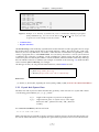
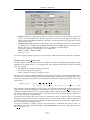
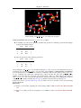
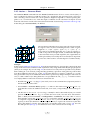
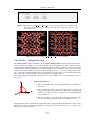
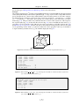
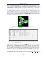
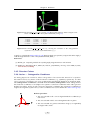
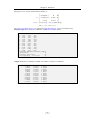
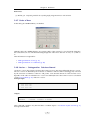
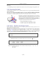
TRAFO — Coordinate
Transformations
U SER M ANUAL
Klaus Eichele
May 14, 2015
— ii —
May 14, 2015
Contents
1 Getting Started
1.1 Introduction . . . . . . . . . . . . . . .
1.2 Overview . . . . . . . . . . . . . . . .
1.2.1 Crystal Axis System Data . . .
1.2.2 Comment Lines . . . . . . . .
1.2.3 Regular Data Lines . . . . . . .
1.3 Revision History . . . . . . . . . . . .
1.4 Known Problems . . . . . . . . . . . .
1.5 Acknowledgements . . . . . . . . . .
1.5.1 Credits . . . . . . . . . . . . . .
1.5.2 Trademark Acknowledgement
1.5.3 Copyright Message . . . . . .
1.5.4 Disclaimer of Warranty . . . .
.
.
.
.
.
.
.
.
.
.
.
.
.
.
.
.
.
.
.
.
.
.
.
.
.
.
.
.
.
.
.
.
.
.
.
.
.
.
.
.
.
.
.
.
.
.
.
.
.
.
.
.
.
.
.
.
.
.
.
.
.
.
.
.
.
.
.
.
.
.
.
.
.
.
.
.
.
.
.
.
.
.
.
.
.
.
.
.
.
.
.
.
.
.
.
.
.
.
.
.
.
.
.
.
.
.
.
.
.
.
.
.
.
.
.
.
.
.
.
.
.
.
.
.
.
.
.
.
.
.
.
.
.
.
.
.
.
.
.
.
.
.
.
.
.
.
.
.
.
.
.
.
.
.
.
.
.
.
.
.
.
.
.
.
.
.
.
.
.
.
.
.
.
.
.
.
.
.
.
.
.
.
.
.
.
.
.
.
.
.
.
.
.
.
.
.
.
.
.
.
.
.
.
.
.
.
.
.
.
.
.
.
.
.
.
.
.
.
.
.
.
.
.
.
.
.
.
.
1
1
1
2
3
3
4
5
5
5
5
5
6
2 Reference
2.1 Help on Menu Items . . . . . . . . . . . . . . . . . . . .
2.2 File Menu . . . . . . . . . . . . . . . . . . . . . . . . . .
2.2.1 File — New . . . . . . . . . . . . . . . . . . . . .
2.2.2 File — Open File . . . . . . . . . . . . . . . . . .
2.2.3 File — Save File As . . . . . . . . . . . . . . . .
2.2.4 File — Exit . . . . . . . . . . . . . . . . . . . . .
2.3 Edit Menu . . . . . . . . . . . . . . . . . . . . . . . . . .
2.3.1 Edit — Undo . . . . . . . . . . . . . . . . . . . .
2.3.2 Edit — Cut . . . . . . . . . . . . . . . . . . . . .
2.3.3 Edit — Copy . . . . . . . . . . . . . . . . . . . .
2.3.4 Edit — Paste . . . . . . . . . . . . . . . . . . . .
2.3.5 Edit — Clear . . . . . . . . . . . . . . . . . . . .
2.3.6 Edit — Select All . . . . . . . . . . . . . . . . . .
2.4 Actions Menu . . . . . . . . . . . . . . . . . . . . . . . .
2.4.1 Action — Generate Positions . . . . . . . . . . .
2.4.2 Symmetry Operations . . . . . . . . . . . . . . .
2.4.3 Action — Generate Block . . . . . . . . . . . . .
2.4.4 Action — Orthogonalize Axes . . . . . . . . . .
2.4.5 Direction Cosines . . . . . . . . . . . . . . . . .
2.4.6 Action — Orthogonalize Coordinates . . . . . .
2.4.7 Order of Axes . . . . . . . . . . . . . . . . . . . .
2.4.8 Action — Orthogonalize: Calculate Normal . .
2.4.9 Cross Product . . . . . . . . . . . . . . . . . . . .
2.4.10 Action — Rotations: Calculate Euler Angles . .
2.4.11 Invert Axis . . . . . . . . . . . . . . . . . . . . .
2.4.12 Euler Angles . . . . . . . . . . . . . . . . . . . .
2.4.13 Rotation Matrices . . . . . . . . . . . . . . . . .
2.4.14 Determining Euler Angles . . . . . . . . . . . . .
2.4.15 Action — Rotations: Euler Rotations Forward .
2.4.16 Action — Rotations: Euler Rotations Backwards
2.4.17 Action — Polar Angles: Calculate . . . . . . . .
2.5 NMR Menu . . . . . . . . . . . . . . . . . . . . . . . . .
2.5.1 Dipolar Second Moment . . . . . . . . . . . . .
2.5.2 Diagonalise (d11 > d22 > d33) . . . . . . . . . .
.
.
.
.
.
.
.
.
.
.
.
.
.
.
.
.
.
.
.
.
.
.
.
.
.
.
.
.
.
.
.
.
.
.
.
.
.
.
.
.
.
.
.
.
.
.
.
.
.
.
.
.
.
.
.
.
.
.
.
.
.
.
.
.
.
.
.
.
.
.
.
.
.
.
.
.
.
.
.
.
.
.
.
.
.
.
.
.
.
.
.
.
.
.
.
.
.
.
.
.
.
.
.
.
.
.
.
.
.
.
.
.
.
.
.
.
.
.
.
.
.
.
.
.
.
.
.
.
.
.
.
.
.
.
.
.
.
.
.
.
.
.
.
.
.
.
.
.
.
.
.
.
.
.
.
.
.
.
.
.
.
.
.
.
.
.
.
.
.
.
.
.
.
.
.
.
.
.
.
.
.
.
.
.
.
.
.
.
.
.
.
.
.
.
.
.
.
.
.
.
.
.
.
.
.
.
.
.
.
.
.
.
.
.
.
.
.
.
.
.
.
.
.
.
.
.
.
.
.
.
.
.
.
.
.
.
.
.
.
.
.
.
.
.
.
.
.
.
.
.
.
.
.
.
.
.
.
.
.
.
.
.
.
.
.
.
.
.
.
.
.
.
.
.
.
.
.
.
.
.
.
.
.
.
.
.
.
.
.
.
.
.
.
.
.
.
.
.
.
.
.
.
.
.
.
.
.
.
.
.
.
.
.
.
.
.
.
.
.
.
.
.
.
.
.
.
.
.
.
.
.
.
.
.
.
.
.
.
.
.
.
.
.
.
.
.
.
.
.
.
.
.
.
.
.
.
.
.
.
.
.
.
.
.
.
.
.
.
.
.
.
.
.
.
.
.
.
.
.
.
.
.
.
.
.
.
.
.
.
.
.
.
.
.
.
.
.
.
.
.
.
.
.
.
.
.
.
.
.
.
.
.
.
.
.
.
.
.
.
.
.
.
.
.
.
.
.
.
.
.
.
.
.
.
.
.
.
.
.
.
.
.
.
.
.
.
.
.
.
.
.
.
.
.
.
.
.
.
.
.
.
.
.
.
.
.
.
.
.
.
.
.
.
.
.
.
.
.
.
.
.
.
.
.
.
.
.
.
.
.
.
.
.
.
.
.
.
.
.
.
.
.
.
.
.
.
.
.
.
.
.
.
.
.
.
.
.
.
.
.
.
.
.
.
.
.
.
.
.
.
.
.
.
.
.
.
.
.
.
.
.
.
.
.
.
.
.
.
.
.
.
.
.
.
.
.
.
.
.
.
.
.
.
.
.
.
.
.
.
.
.
.
.
.
.
.
.
.
.
.
.
.
.
.
.
.
.
.
.
.
.
.
.
.
.
.
.
.
.
.
.
.
.
.
.
.
.
.
.
.
.
.
7
7
8
8
8
8
8
8
9
9
9
9
9
9
10
10
10
16
17
20
20
22
22
23
23
24
24
25
27
27
28
28
29
29
30
.
.
.
.
.
.
.
.
.
.
.
.
.
.
.
.
.
.
.
.
.
.
.
.
.
.
.
.
.
.
.
.
.
.
.
.
.
.
.
.
.
.
.
.
.
.
.
.
— iii —
May 14, 2015
.
.
.
.
.
.
.
.
.
.
.
.
.
.
.
.
.
.
.
.
.
.
.
.
.
.
.
.
.
.
.
.
.
.
.
.
.
.
.
.
.
.
.
.
.
.
.
.
.
.
.
.
.
.
.
.
.
.
.
.
Contents
2.5.3
Diagonalise (s11 < s22 < s33)
. . . . . . . . . . . . . . . . . . . . . . . . . . . .
3 Applications
3.1 Dealing with NMR Tensors . . . . . . . . . . . . .
3.1.1 The Absolute Magnetic Shielding Tensor .
3.1.2 The Electric Field Gradient Tensor . . . . .
3.1.3 Transforming the CSA into the EFG frame
— iv —
May 14, 2015
.
.
.
.
.
.
.
.
.
.
.
.
.
.
.
.
.
.
.
.
.
.
.
.
.
.
.
.
.
.
.
.
.
.
.
.
.
.
.
.
.
.
.
.
.
.
.
.
.
.
.
.
.
.
.
.
.
.
.
.
.
.
.
.
.
.
.
.
.
.
.
.
.
.
.
.
.
.
.
.
.
.
.
.
30
31
31
31
32
34
1 Getting Started
This chapter covers the following topics:
Introduction
An introduction to Trafo
Overviews
An overview of some of the common tasks and actions
Revision History
Summary of changes versus previous versions
Known Problems
Summary of known problems
Acknowledgements Credits for important contributions etc.
1.1 Introduction
Trafo is a program to perform coordinate transformations useful in combination with the analysis of
single-crystal NMR spectra, as well as to assist in some related procedures such as diagonalizations
of tensors. Although Trafo will often deal with crystallographic data, it is not smart in that respect;
it is a simple tool and not an expert system. If you are looking for powerful software to deal with
crystallographic questions, consider Platon or Mercury, both available freely.
Trafo is part of a simulation package developed during my stay at the Department of Chemistry,
Dalhousie University, Halifax, Canada. The initial version has been written in C++ using Borland
C++ 4.52 and has been developed to run on IBM-compatible personal computers under the MSWindows environment in the 16-bit subsystem. For the 32-bit version, Borland C++ 5.0 has been used
initially. The current version has been produced using Microsoft Visual C++ 2008 Express Edition.
1.2 Overview
The actions selected by the menu commands operate
• either directly on the content of the edit window - the default if there is anything available
• or, if the edit window is empty (you can select File—New (p. 8) to clear the window), on an
input file, the name of which is requested from the user.
The output is almost always directed to an output file, the name of which is also asked for. Note
that currently the edit window has a limited capacity of about 64 KB, which is sufficient for most
operations, but can be exceeded easily after application of Action—Generate Block (p. 16); there ´ıs
no such low limit on file oriented operations.
The format of the input data should conform to the format expected by Alchemy for crystal data files,
although Trafo is a little more flexible in this respect. I have chosen this file format because in the 90ties, when I started the development of Trafo, we used the molecular modeling programs Alchemy II
and Alchemy 3 to visualize molecules and the results of single crystal NMR data. Another advantage
of this file format is its simplicity. An example is shown in Fig. 1.1. Several of the examples shown
later in this document use this example as starting point, hence you could copy and paste the data in
the figure into Trafo and save them for perusal later.
Crystal data files to be recognized by Alchemy must have the extension ”.CRY”. All operations are
line-oriented, i.e., each line of the ASCII-type data forms one data record. Basically, there are three
different types of data records, each of them with some restrictions as to their format. The three data
types are:
• Crystal axis: crystal system data
—1—
May 14, 2015
Chapter 1. Getting Started
7.502 7.502 7.546 90.00 90.00 90.00
P 0.000 0.000 0.000
N 0.000 0.000 0.500
O 0.085 0.146 0.115
H 0.014 0.111 0.573
H 0.227 0.146 0.122
/* crystal structure of NH4H2PO4
/* space group: I-42d (No. 122)
/* neutron diffraction data
/* Tenzer, L.; Frazer, B.L.; Pepinsky, R.
/* Acta Cryst. 1958, 11, 505
*/
*/
*/
*/
*/
Figure 1.1: Example of an Alchemy crystal data file, here for ammonium dihydrogen phosphate
(ADP), NH4 H2 PO4 [1]. You can save the data as ADP 01 fract coord.cry if you want
to repeat some of the example actions shown later.
• Comment lines
• Regular data lines
One disadvantage of the Alchemy crystal data file format is that most other programs do not accept
this format. Most of them will be able to deal with Alchemy ”.MOL” files, but not the ”.CRY” files.
However, it is not very difficult to convert the ”.CRY” files into a format that is recognized by a wider
variety of programs, the so called XYZ format. You can always use Trafo to convert your fractional
coordinates into Cartesian coordinates. In the resulting file, simply replace the first line with the
Cartesian crystal axes data by the number of atoms in the file, add a second line with a title, and keep
the rest with the Cartesian coordinates (an example of a XYZ file is shown in Fig. 2.4). Such XYZ files
can be read into Jmol or Mercury, for example.
On this type of data, one can perform transformations, called Actions in Trafo.
Links to some of the software mentioned:
• Jmol: http://www.jmol.org
• Mercury: http://www.ccdc.cam.ac.uk/mercury
References:
(1) Tenzer, L.; Frazer, B.L.; Pepinsky, R. Acta Crystallogr. 1958, 11, 505, DOI: 10.1107/S0365110X58001389
1.2.1 Crystal Axis System Data
The data line with crystal axes data describes the geometry of the unit cell of a crystal and consists
of six floating point numbers, a, b, c, α, β, γ, where:
a, b, c:
˚
length of the respective crystal axis in Angstrøm
α, β, γ:
angle between pairs of crystal axes (α is the angle
between b and c, β between a and c, and γ between
a and b).
For Cartesian coordinates, this line will read:
1.0 1.0 1.0 90.0 90.0 90.0
Note: This data line is required for many operations and has always to be the first line in this case.
For actions where this line is not required, it is optional but, if present, it also has to be the first line!
—2—
May 14, 2015
Chapter 1. Getting Started
1.2.2 Comment Lines
Comment lines can be added to the data in order to assist later in identifying the data set. In Alchemy,
comment lines can only be added to the end of the data set, but in Trafo they may appear anywhere
(except for the first line in cases where crystal axis system data are required). Comment lines are
written in the same format as comment lines in the C programming language, as the following example illustrates:
/* this is a C−type comment line */
In order to qualify as a comment line, the first two characters of the line have to be a slash (/) and an
asterisk (*).
1.2.3 Regular Data Lines
Each line with regular coordinate data consists of four data entries, all of them are required. The
general format will be:
LABEL x.xxxx −y.yyyy z.zzzz
where:
LABEL a label of at least 1 and up to 6 characters describing the atom or data type (no spaces or
other whitespace characters, e.g. tabs, within this name are allowed, but underscores etc.); for
use with Alchemy, the label should specify a valid Alchemy atom type, but Trafo does not care.
x,y,z the x, y, z coordinates as floating point numbers in free format
A special type of data line will be recognized by Trafo, which is a line describing the origin of the
coordinate system:
OR x.xxx y.yyy z.zzz
where Trafo doesn’t really care about the coordinates (right now), but this line shall usually be neglected (the position and number of such lines doesn’t matter either).
The purpose of this origin is to serve as starting point for the display of principal axes systems, e.g., of
chemical shift tensors, whereby the directions of the principal components were indicated as dummy
˚ away from the origin.
atoms, e.g., d11, d22, d33, that are 1 A
—3—
May 14, 2015
Chapter 1. Getting Started
1.3 Revision History
This page summarizes the changes made compared to previous versions of Trafo. Experienced users
may use this information as a quick update on new program features.
New in Version 2.5.7 (14.05.2015):
• new feature: the help file contains a lot of examples that illustrate the use of Trafo.
• new feature: the help file is now in PDF format because it is suitable for both online viewing
as well as printing. To view or print this documentation, any PDF viewer should work. Also,
most viewers should be able to deal with the hyperlinks that cross-link topics in this help file.
However, opening a PDF file at a specified position is more complicated. Therefore, not every
PDF viewer will work with Trafo to display context sensitive help. This matter is aggravated
by the fact that every viewer has its own mechanism! Currently, context sensitive help should
work with the following PDF viewers:
– Adobe uses with its Acrobat Reader series of products a mechanism called Dynamic Data
Exchange (DDE) to open a PDF file at a specific position. For ages, the name of the DDE
server has been acroview. However, with the introduction of Acrobat Reader X this tradition has been broken on purpose, breaking many applications that rely on this mechanism.
Trafo should be able to work with older versions of the Acrobat Reader as well as with the
acroviewR10 DDE server of Adobe Reader X. Because I have been quite dissatisfied with
the Adobe products from Reader 5 onwards, I am using a different PDF viewer and will
not always check whether Acrobat is still working!
– My preferred PDF viewer is the free PDFXChangeEditor, the successor of PDFXChangeViewer
by Tracker Software Products, Ltd. (http://www.tracker-software.com), more powerful and reliable than the Acrobat Reader. The opening of a PDF file at a specific position is
achieved via command line parameters.
– Another viewer used by people working with LATEX is the Sumatra PDF Viewer (http:
//blog.kowalczyk.info/software/sumatrapdf), also supported by Trafo.
– Other PDF viewers such as FoxIt or NitroPDF do not support DDE or command line parameters, as far as I know.
• bug fix: a few superfluous new lines produced in the output files got eaten now.
New in Version 2.5.3 (21.01.2009):
• converted project to Microsoft Visual C++ 2008 Express Edition
• added diagonalization functions for single crystal NMR
• some minor bug fixes
New in Version 2.4.7 (30.04.2004):
• some minor bug fixes
New in Version 2.4.3:
• this is the first release with a 32 bit version; some internal changes
• comment lines are now copied to output file
New in Version 2.3.2:
• added calculation of dipolar second moments
• better error reporting
New in Version 2.2.10:
• Added calculation of normals.
—4—
May 14, 2015
Chapter 1. Getting Started
1.4 Known Problems
None right now.
1.5 Acknowledgements
This section covers the following topics:
Credits
Credits for important contributions
Trademarks
Trademark acknowledgements
Copyright
The obligatory copyright statement
Disclaimer
The obligatory disclaimer message
1.5.1 Credits
• Microsoft for providing Visual C++ 2008 Express Edition for free
• Jordan Russell for making Inno Setup available (http://www.jrsoftware.org/)
• Jochen Kalmbach for demonstrating how to statically link against the Microsoft CRT and thus
get rid of VCREDIST X86.EXE (http://blog.kalmbach-software.de)
• “chicks” for demonstrating in his pdfp PDF tools how to establish Dynamic Data Exchange
(DDE) with Adobe Acrobat (Reader) (http://www.esnips.com/web/PDFTools)
• This manual has been produced using the MiKTEX (http://www.miktex.org) distribution of
LATEX in combination with the TeXstudio editor (http://texstudio.sourceforge.net/).
• Irfan Skiljan’s IrfanView (http://www.irfanview.com/) has been used to process bitmapped
images, and Inkscape (www.inkscape.org) for dealing with vector graphics.
1.5.2 Trademark Acknowledgement
• Microsoft (MS) is a registered trademark and MS−DOS, MS−Word and MS−Windows are trademarks of Microsoft Corporation.
• Alchemy is a copyrighted program and registered trademark of TRIPOS Associates, Inc., a subsidiary of Evans & Sutherland.
• Other brand and/or product names are used for identification purposes only and are trademarks, registered trademarks or copyrights of their respective owners.
1.5.3 Copyright Message
Copyright © 1995,2015 Klaus Eichele. All rights reserved.
This program executable, help file and related files may be distributed freely and may
be used without fee by any individual for non-commercial use and by any government organization. Although the copyright holder retains all rights to this document
and the software package, you are allowed to copy and distribute verbatim copies of
them, as you received them, in any medium, provided that you conspicuously and
appropriately publish on each copy an appropriate copyright notice and disclaimer
of warranty; keep intact all the notices that refer to this license and to the absence of any warranty;
and distribute a copy of this license along with it.
This package may not be distributed as a part of any commercial package.
You are expressly not allowed to sell or license this package!
—5—
May 14, 2015
Chapter 1. Getting Started
1.5.4 Disclaimer of Warranty
Because this software package is licensed free of charge, there is no warranty, to the extent permitted by applicable law. This package is provided “as is”, without warranty of any kind, either
expressed or implied, including, but not limited to, the implied warranties of merchantability and
fitness for a particular purpose; the entire risk as to the quality and performance of the contents
of this package is with you; should this package prove defective, you assume the cost of all necessary servicing, repair, or correction; in no event, unless required by applicable law or agreed
to in writing, will any copyright holder, or any other party who may modify and/or redistribute
this package, as permitted in the license, be liable to you for damages, including any general,
special, incidental or consequential damages arising out of the use or inability to use the package
(including but not limited to loss of data or data being rendered inaccurate or losses sustained by
you or third parties), even if such holder or other party has been advised of the possibility of such
damages. In any case, liability will be limited to the amount of money that the copyright holder
received from you for the use of this program.
—6—
May 14, 2015
2 Reference
2.1 Help on Menu Items
The menu system of Trafo consists of the following pop−up menus:
Category
Menu Item
File
File and document management:
Edit
Action
Action
New (p. 8)
clears the content of the Trafo edit window
Open... (p. 8)
read a file into Trafo s edit window
Save as... (p. 8)
save the content of the edit window to a new file
Exit (p. 8)
exit Trafo
Editor window actions:
Undo (p. 9)
undo last changes
Cut (p. 9)
cut selection into clipboard
Copy (p. 9)
copy selection into clipboard
Paste (p. 9)
insert content of clipboard
Clear (p. 9)
clear content
Select All (p. 9)
select all content
Perform transformations:
Generate:
10)
Positions (p.
generate symmetry related sites
Generate: Block (p. 16)
generate a cube of several unit cells
Orthogonalize: Axes (p.
17)
transform an oblique axis set into an orthogonal
set
Orthogonalize:
nates (p. 20)
transform coordinates from an oblique system
into a Cartesian system
Coordi-
Orthogonalize: Calculate
normal (p. 22)
calculate the normal vector
Rotations: Calculate Euler
Angles (p. 23)
calculate Euler Angles from direction cosines
Rotations: Euler Rotations
Forwards (p. 27)
transform from the old system into the new system
Rotations: Euler Rotations
Backwards (p. 28)
transform from the new system into the old system
—7—
May 14, 2015
Chapter 2. Reference
Polar angles: Calculate (p.
28)
NMR
convert Cartesian coordinates into polar coordinates
Perform some NMR relevant calculations:
Dipolar Moment (p. 29)
calculates dipolar second moments for singlecrystal or powder samples
Diagonalise (d11 > d22 >
d33) (p. 30)
diagonalise a general chemical shift tensor
Diagonalise (s11 < s22 <
s33) (p. 30)
diagonalise a general magnetic shielding tensor
2.2 File Menu
The File pop-up menu consists of the following items:
2.2.1 File — New
Execution of the command New in the File popup menu clears the edit window. If the current
content of the edit window has been modified but not saved, the user has the choice of writing the
current content of the edit window to a file. Once the data are gone, they are gone!
2.2.2 File — Open File
Execution of the command Open in the File popup menu retrieves the content of a data file into the
edit window. If the current content of the edit window has been modified but not saved, the user has
the choice of writing the current content of the edit window to a file. Once the data are gone, they
are gone!
2.2.3 File — Save File As
Execution of the command Save as in the File popup menu saves the content of the edit window, if
available, into a data file. To prevent Trafo from adding the extension .cry, enclose your file name in
double quotes.
N.B. It overwrites existing data files without a warning!
2.2.4 File — Exit
Execution of the command Exit in the File popup menu quits Trafo. If the current content of the edit
window has been modified but not saved, the user has the choice of writing the current content of
the edit window to a file. Once the data are gone, they are gone!
2.3 Edit Menu
The Edit Menu provides various commands which act on the content of the edit window. Depending
on previous actions, not all commands might be available at a given time. In their functionality, the
commands are typical of a Windows application.
—8—
May 14, 2015
Chapter 2. Reference
The Edit pop-up menu consists of the following items:
2.3.1 Edit — Undo
This command restores the file in the current window to the way it was before your most recent edit
or cursor movement. Undo inserts any characters you deleted, deletes any characters you inserted,
replaces any characters you overwrote, and moves your cursor back to a prior position.
This command is available only if an Edit window is currently active and there is something to undo.
2.3.2 Edit — Cut
This command removes the selected text from your document and places the text in the Clipboard.
You can then choose Edit|Paste to paste the cut text into any other document (or somewhere else in
the same document). You can paste the cut text as many times as you want until you choose Edit|Cut
or Edit|Copy.
This command is available only if an Edit window is currently active and text has been marked for
selection.
2.3.3 Edit — Copy
This command leaves the selected text intact and places an exact copy of it in the Clipboard. To paste
the copied text into any other document, choose Edit|Paste.
To copy text from a Help window, display the text you want to copy, then select Edit|Copy. The
entire contents of the window is copied to the Clipboard.
This command is only available if an Edit window is currently active and text has been marked for
selection.
2.3.4 Edit — Paste
This command inserts the contents of the Clipboard into the current window at the cursor position.
This command is available only if an Edit window is currently active and there is something to paste.
2.3.5 Edit — Clear
This command removes the selected text but does not copy it to the Clipboard. This means you
cannot paste the text as you could if you had chosen Edit|Cut or Edit|Copy.
Although you cannot paste the cleared text, you can undo the Clear command with Edit|Undo.
Clear is useful if you want to delete text, but you do not want to overwrite text held in the Clipboard.
This command is available only if an Edit window is currently active and text has been marked for
selection.
2.3.6 Edit — Select All
This command selects the entire contents of the active Edit window. You can then use Edit|Copy or
Edit|Cut to copy it to the Clipboard, or perform any other editing action.
This command is available only if an Edit window is currently active.
—9—
May 14, 2015
Chapter 2. Reference
2.4 Actions Menu
The Actions Menu combines all the commands to perform transformations on input data. Currently,
the following actions can be performed:
2.4.1 Action — Generate Positions
The Generate Positions command from the Actions|Generate menu allows to create new coordinates (positions) from the existing one by applying symmetry operations.
One possible application is to create all the molecules within the unit cell from the fractional crystal
coordinates of one given molecule and applying the generating symmetry operations on them, as
detailed in [1]. Also, after generating one complete unit cell, one could create a cube of unit cells by
using the Generate Block (p. 16) command from the Actions|Generate menu.
For example, consider the situation illustrated in the figure. The goal is to generate a new molecule which is related to the current one by a twofold screw axis operation.
Such a symmetry operation requires the rotation of atomic
positions by 180°about the axis of the screw, followed by
a translational element. The detailed procedure together
with some examples is explained in the topic symmetry
operations (p. 10).
References:
[1] International Tables for X−ray Crystallography, Kynoch Press: Birmingham, England, 1974; Vol. 1.
2.4.2 Symmetry Operations
The Generate Positions command from the Actions|Generate menu allows to create new coordinates (positions) from the existing ones by applying symmetry operations. One application is to
generate all positions in the unit cell from the content of the asymmetric unit. It calls the dialog box
Symmetry Operations. A detailed example at the bottom of this topic illustrates the procedure.
In the dialog box Symmetry Operations, one defines:
— 10 —
May 14, 2015
Chapter 2. Reference
• Number of sites to be generated: In order to generate a unit cell, enter the number of molecules
(or sites or formula units) as the number of positions. For the first site, apply the identity operation (which is the default symmetry operation). For the following sites, apply the necessary
symmetry operations.
• Symmetry operation required to generate the sites: The symmetry operations can be written
as combinations of multiplications (Factor) and summations (Shift) applied to the input coordinates, where it is possible that the source of coordinates are interchanged.
The general equation to calculate the new coordinates is:
New(k) = Factor × Old(m) + Shift
with k,m = x, y, z.
It is easier to apply symmetry operations on fractional coordinates rather than Cartesian coordinates.
Example: Space Group I42d (No. 122)
For this example, we shall use the fractional coordinates of ammonium dihydrogen phosphate (ADP),
NH4 H2 PO4 , presented in Fig. 1.1 as a starting point. This example is sufficiently complex to illustrate
quite a few points:
• the application of simple symmetry operations;
• how to deal with special positions;
• why it could be necessary to change the source.
The space group symbol I indicates that the crystal structure of ADP is a body centered lattice, therefore there is a so-called centering operation that generates this centered part. Altogether, there are 16
symmetry related general positions, half of them generated by this centering operation. This can be
expressed as:
(0, 0, 0; ½,½,½) + ( x, y, z; x, y, z; y, x, z; y, x, z;
½ − x, y, ¼ − z; ½ + x, y, ¼ − z; ½ + y, x, ¼ + z; ½ − y, x, ¼ + z)
(2.1)
This generally adopted setting for ADP (at least, the researchers that determined the structure of
ADP called it “generally adopted”) is obtained by a rotation of 90° about the 4 axis relative to the
setting in International Tables for X-ray Crystallography (1965) for the space group I42d [1,2]. If you use
the setting found in the International Tables to generate the positions of ADP from the coordinates in
Fig. 1.1, you will get a wrong structure!
To generate all 16 general positions of ADP, we will take two steps: in the first step, we will apply
the eight operations shown in the second part of Eq. 2.1 and save the result to a file. In this file, we
will need to clean up a few positions related to the special positions of P and N before application of
the second step, the centering operation.
If you have not done so already, generate your starting file as outlined in the caption of Fig. 1.1.
Read this file into Trafo and select Action — Generate Positions. As name for the output file, enter
ADP 02 unithalf.cry.
— 11 —
May 14, 2015
Chapter 2. Reference
¶ For now, we want to generate eight positions, hence we enter 8 in No. of Positions. For the
first position, already queried in this dialog box, the identity operation is used, with a factor
of 1 and a shift of zero for all coordinates X,Y,Z (this operation is the default), with the source
being x, y, and z, respectively. This simply copies the input coordinates into the output file. To
generate this position, the default looks like:
factor
shift
source
X:
1.0
0.0
x
Y:
1.0
0.0
y
Z:
1.0
0.0
z
Click OK.
· The second position is related to the first by a two-fold rotation around the 4 axis (the 4 axis
generates a two-fold axis), expressed in Eq. 2.1 as x, y, z. To generate this position, enter:
factor
shift
source
X:
-1.0
0.0
x
Y:
-1.0
0.0
y
Z:
1.0
0.0
z
¸ The third position, generated by y, x, z, interchanges the sources for x and y:
factor
shift
source
X:
-1.0
0.0
y
Y:
1.0
0.0
x
Z:
-1.0
0.0
z
¹ The fourth position, generated by y, x, z, is produced by:
factor
shift
source
X:
1.0
0.0
y
Y:
-1.0
0.0
x
Z:
-1.0
0.0
z
º The fifth position, generated by ½ − x, y, ¼ − z, is produced by:
factor
shift
source
X:
-1.0
0.5
x
Y:
1.0
0.0
y
Z:
-1.0
0.25
z
» The sixth position, generated by ½ + x, y, ¼ − z, is produced by:
factor
shift
source
X:
1.0
0.5
x
Y:
-1.0
0.0
y
Z:
-1.0
0.25
z
¼ The seventh position, generated by ½ + y, x, ¼ + z, is produced by:
— 12 —
May 14, 2015
Chapter 2. Reference
factor
shift
source
X:
1.0
0.5
y
Y:
1.0
0.0
x
Z:
1.0
0.25
z
½ The eigth position, generated by ½ − y, x, ¼ + z, is produced by:
factor
shift
source
X:
-1.0
0.5
y
Y:
-1.0
0.0
x
Z:
1.0
0.25
z
Open the resulting file, ADP 02 unithalf.cry, in Trafo. Because we have applied the symmetry
operations on all atoms, including P and N at special positions, we have generated too many N and
P positions. There are four formula units of ADP per unit cell, hence our first 8 symmetry operations
should generate two formula units: 2 · NH4 H2 PO4 = N2 H8 H4 P2 O8 (the protons at oxygen have only
an occupation no. of one half). Only one quarter of the P and N positions are required. You can see
that P positions 2-4 are the same as the first and 6-8 the same as the fifth, hence can be deleted, leaving
two P positions, as required. It is a little more complicated for nitrogen: positions 2,6 are the same as
1 and 5, while 3,4,7,8 correspond to 1 and 5, but shifted by one unit of the c cell axis, therefore they
are also superfluous. Clean up the file as outlined and save the result again as ADP 02 unithalf.cry.
The result should look like Fig. 2.1.
Now we shall generate the second half of the unit cell by applying the centering operation. With file
ADP 02 unithalf.cry in the edit window of Trafo or specifying this file as input file, select Action —
7.502
P
N
O
H
H
O
H
H
O
H
H
O
H
H
P
N
O
H
H
O
H
H
O
H
H
O
H
H
7.502 7.546
0.000000
0.000000
0.085000
0.014000
0.227000
-0.085000
-0.014000
-0.227000
-0.146000
-0.111000
-0.146000
0.146000
0.111000
0.146000
0.500000
0.500000
0.415000
0.486000
0.273000
0.585000
0.514000
0.727000
0.646000
0.611000
0.646000
0.354000
0.389000
0.354000
90.00 90.00
0.000000
0.000000
0.146000
0.111000
0.146000
-0.146000
-0.111000
-0.146000
0.085000
0.014000
0.227000
-0.085000
-0.014000
-0.227000
0.000000
0.000000
0.146000
0.111000
0.146000
-0.146000
-0.111000
-0.146000
0.085000
0.014000
0.227000
-0.085000
-0.014000
-0.227000
90.00
0.000000
0.500000
0.115000
0.573000
0.122000
0.115000
0.573000
0.122000
-0.115000
-0.573000
-0.122000
-0.115000
-0.573000
-0.122000
0.250000
-0.250000
0.135000
-0.323000
0.128000
0.135000
-0.323000
0.128000
0.365000
0.823000
0.372000
0.365000
0.823000
0.372000
Figure 2.1: Alchemy crystal data file for ammonium dihydrogen phosphate (ADP), NH4 H2 PO4 , generated from the data in Fig. 1.1, corresponding to one half of the unit cell. Save the data as
ADP 02 unithalf.cry if you want to repeat some of the example actions shown later.
— 13 —
May 14, 2015
Chapter 2. Reference
Figure 2.2: File "ADP 03 unit cart.xyz" displayed using Jmol.
Generate Positions and specify ADP 03 unit.cry as output.
¾ As number of positions we specify 2, and the first operation as identity operation shall simply
copy the first eight positions:
factor
shift
source
X:
1.0
0.0
x
Y:
1.0
0.0
y
Z:
1.0
0.0
z
¿ The last operation is the centering operation:
factor
shift
source
X:
1.0
0.5
x
Y:
1.0
0.5
y
Z:
1.0
0.5
z
The resulting file ADP 03 unit.cry should look like Fig. 2.3. If you are curious what kind of result we
produced, you can load ADP 03 unit.cry into Trafo, select Action — Orthogonalize: Coordinates
to convert fractional coordinates into Cartesian coordinates and save the result as ADP 03 unit cart.cry. Read this file, delete the comment lines, replace the first line (the unit cell data) by the
number of atoms in the file, 56, insert a second line with a title, e.g., ADP, and save the result as
"ADP 03 unit cart.xyz" (note the double quotes; they prevent Trafo from adding the extension
.CRY). You can read this XYZ file into Jmol (p. 2), and the result should look like Fig. 2.2.
In the next section, Generate: Block (p. 16), we shall see how to use this as base for generating
packing diagrams.
References:
(1) Tenzer, L.; Frazer, B.L.; Pepinsky, R. Acta Crystallogr. 1958, 11, 505, DOI: 10.1107/S0365110X58001389.
(2) Khan, A. A.; Baur, W. H. Acta Crystallogr., Sect. B 1973, 29, 2721, DOI: 10.1107/S0567740873007442.
— 14 —
May 14, 2015
Chapter 2. Reference
7.502
P
N
O
H
H
O
H
H
O
H
H
O
H
H
P
N
O
H
H
O
H
H
O
H
H
O
H
H
P
N
O
H
H
O
H
H
O
H
H
O
H
H
P
N
O
H
H
O
H
H
O
H
H
O
H
H
7.502 7.546
0.000000
0.000000
0.085000
0.014000
0.227000
-0.085000
-0.014000
-0.227000
-0.146000
-0.111000
-0.146000
0.146000
0.111000
0.146000
0.500000
0.500000
0.415000
0.486000
0.273000
0.585000
0.514000
0.727000
0.646000
0.611000
0.646000
0.354000
0.389000
0.354000
0.500000
0.500000
0.585000
0.514000
0.727000
0.415000
0.486000
0.273000
0.354000
0.389000
0.354000
0.646000
0.611000
0.646000
1.000000
1.000000
0.915000
0.986000
0.773000
1.085000
1.014000
1.227000
1.146000
1.111000
1.146000
0.854000
0.889000
0.854000
90.00 90.00
0.000000
0.000000
0.146000
0.111000
0.146000
-0.146000
-0.111000
-0.146000
0.085000
0.014000
0.227000
-0.085000
-0.014000
-0.227000
0.000000
0.000000
0.146000
0.111000
0.146000
-0.146000
-0.111000
-0.146000
0.085000
0.014000
0.227000
-0.085000
-0.014000
-0.227000
0.500000
0.500000
0.646000
0.611000
0.646000
0.354000
0.389000
0.354000
0.585000
0.514000
0.727000
0.415000
0.486000
0.273000
0.500000
0.500000
0.646000
0.611000
0.646000
0.354000
0.389000
0.354000
0.585000
0.514000
0.727000
0.415000
0.486000
0.273000
90.00
0.000000
0.500000
0.115000
0.573000
0.122000
0.115000
0.573000
0.122000
-0.115000
-0.573000
-0.122000
-0.115000
-0.573000
-0.122000
0.250000
-0.250000
0.135000
-0.323000
0.128000
0.135000
-0.323000
0.128000
0.365000
0.823000
0.372000
0.365000
0.823000
0.372000
0.500000
1.000000
0.615000
1.073000
0.622000
0.615000
1.073000
0.622000
0.385000
-0.073000
0.378000
0.385000
-0.073000
0.378000
0.750000
0.250000
0.635000
0.177000
0.628000
0.635000
0.177000
0.628000
0.865000
1.323000
0.872000
0.865000
1.323000
0.872000
Figure 2.3: Alchemy crystal data file for ammonium dihydrogen phosphate (ADP), NH4 H2 PO4 , generated from the data file shown in Fig. 2.1, corresponding to the unit cell content. Save the
data as ADP 03 unit.cry if you want to repeat some of the example actions shown later.
— 15 —
May 14, 2015
Chapter 2. Reference
2.4.3 Action — Generate Block
The Generate Block command from the Actions|Generate menu allows to create a block (cube) of
new coordinates (positions) around the existing one. Specifically, this generates from a unit cell a
cube consisting of several unit cells. Such operations might be required to construct packing diagrams or as a convenient tool to create the input coordinates for the calculation of dipolar second
moments. The entire content of the unit cell itself should be created using Generate Positions (p. 10).
In the dialog box Generate Block, one defines:
The parameter n describes how many unit cells will get created.
For a given value of n, this command generates a cube of corner
length 2n + 1, or (2n + 1)(2n + 1)(2n + 1) − 1 = (2n + 1)3 − 1
new positions around the input data. For a value of n equal to 1,
a cube of 27 positions will get created, as indicated in the figure
to the left. In the newly created output file, the original data set
will be placed first, followed by the new data (this is important
for later use of the results to calculate dipolar second moments).
Example:
In the section Symmetry Operations (p. 10) we demonstrated how to generate the content of the unit
cell given the fractional coordinates of the asymmetric unit, using ammonium dihydrogen phosphate
(ADP) as an example. If you look at Fig. 2.2, the result is not exactly what is expected naively. Rather
than resulting in a sort of block, such generating symmetry operations often generate positions that
lie in the neighboring unit cell (e.g., in Fig. 2.3 all atoms that have a negative coordinate or a coordinate greater than one). We would need to shift all these positions by integer multiples of the unit cell
axes (i.e. add or subtract 1) to bring them into our expected block of 0 ≤ x, y, z ≤ 1. Another solution
is to simply add more unit cells around our central unit cell:
• Read file ADP 03 unit.cry (Fig. 2.3) into Trafo, remove the comment lines (if present) and save
the file under the same name.
• Select Action — Generate Block, specify n = 1 and save the result as ADP 04 unit block.cry.
Note that this creates 26 additional unit cells, 27 in total, corresponding to 1512 atomic positions.
• The file ADP 04 unit block.cry is too big (> 64 KB) for Trafo’s edit window, but you can still
perform file related actions. E.g., to visualize this new result, clear the Trafo edit window
(File — New) and select Action — Orthogonalize: Coordinates, leave the order of axes at
their defaults, specify ADP 04 unit block.cry as input file and ADP 04 unit block cart.cry
as output file. Copy this file to ADP 04 unit block cart.xyz and use an editor that has a higher
capacity as Trafo (the Windows editor Notepad will do) to replace the Cartesian crystal data
line by the number of atoms, 1512, and insert a second line with a title (c.f. Fig. 2.4). Save the
file and open it in Jmol (p. 2). Two different views of the result are shown in Fig. 2.5.
— 16 —
May 14, 2015
Chapter 2. Reference
1512
ADP 27 unit cells
P
0.000000
N
0.000000
O
0.637670
H
0.105028
...
0.000000
0.000000
1.095292
0.832722
0.000000
3.773000
0.867790
4.323858
Figure 2.4: Beginning of file ADP 04 unit block cart.xyz, showing the structure of an XYZ file: number of atoms in the first line, a second line with a title, followed by the Cartesian coordinates of the atoms.
Figure 2.5: Two views of file ADP 04 unit block cart.xyz using Jmol.
2.4.4 Action — Orthogonalize Axes
The Orthogonalize Axes command from the Actions|Orthogonalize menu orthogonalizes the direction cosines of an oblique axis system in the order given by Rollett’s procedure. This is an action
required when dealing with single crystal NMR. Typically, in this experiment a crystal is mounted
in some holder and X-ray diffraction is used to determine the orientation of the crystal axes with
respect to the holder. If the crystal axes form an oblique system, i.e., at least one angle differs from
90 °, it is useful to transform them into an orthogonal axes set, because one can then determine the
Euler angles (p. 24) that relate the crystal axes to the crystal holder frame.
This action requires to assign the crystal axes a,b,c to the coordinate axes X,Y,Z to define the order of
axes (p. 22).
Rollett’s procedure [1]:
1. The axis selected as the c axis is aligned with the coordinate system Z axis.
2. The axis selected as the b axis is brought into the YZ plane. To
orthogonalize this axis, the normal n to the bc plane is determined
as the cross product (p. 23) b x c, the new b* axis results from the
cross product c x n.
3. The axis selected as a usually points somewhere along the X direction. The orthogonalized a* is the cross product of b* x c.
The input data need to contain three regular data lines corresponding to the direction cosines of the
oblique axis system. All following data lines are ignored. Crystal axes data lines (p. 2) and origin
data lines (p. 3) are neglected.
— 17 —
May 14, 2015
Chapter 2. Reference
See also the topic Orthogonalize Coordinates (p. 20) for more information.
Example:
The example results from a 31 P single-crystal NMR experiment on (5-methyldibenzophosphole)pentacarbonylmolybdenum(0) and has been published [2]. A large crystal of this compound has been
grown and glued onto a hollow three-sided alumina cube measuring 4 mm on each side. Using X˚ b = 7.7917(5)
ray diffraction, the orientation of the monoclinic crystal axis system (a = 31.113(2) A,
˚
A, c = 17.9522(12), β = 122.135(4)°, space group C2/c) with respect to this cube frame was determined (Fig. 2.6). This procedure also yields the direction cosines of the crystal axes with respect to
the crystal holder (Fig. 2.7). In the data file shown in Fig. 2.7, I have included the cube frame x, y, z
˚ away from the origin, OR). We can easily convert this to a XYZ file (compare Fig. 2.4),
axes (but 1.5 A
but Mercury (p. 2) or Jmol (p. 2) will not be able to deal with the result properly. The reason is that
we are specifying “atoms” (OR, a, x, z) that are unknown to those programs. One way around this is
to replace them by sensible atoms, e.g., the XYZ file displayed in Fig. 2.8.
Figure 2.6: Orientation of the monoclinic crystal axes a, b, c in the crystal holder frame x, y, z.
1.00 1.00 1.00 90.00 90.00 90.00
or 0.00000
0.00000
0.00000
a
0.91826
0.31965 -0.23380
b -0.18295
0.87884
0.43607
c -0.19058 -0.46992
0.86036
x 1.5 0.0 0.0
y 0.0 1.5 0.0
z 0.0 0.0 1.5
/* (OC)5Mo(Me-DBP)
*/
/* crystal axis system in
*/
/* cube axis system
*/
Figure 2.7: File MoMeDBP 01 crys cube.cry, showing the orientation of the monoclinic crystal axes
a, b, c in the crystal holder frame x, y, z.
7
(OC)5Mo(Me-DBP) crystal axis system in cube axis system
C
0.00000
0.00000
0.00000
H 0.91826
0.31965 -0.23380
H -0.18295
0.87884
0.43607
H -0.19058 -0.46992
0.86036
Cl 1.5 0.0 0.0
Cl 0.0 1.5 0.0
Cl 0.0 0.0 1.5
Figure 2.8: File MoMeDBP 01 crys cube.xyz, showing the orientation of the monoclinic crystal axes
a, b, c in the crystal holder frame x, y, z.
— 18 —
May 14, 2015
Chapter 2. Reference
However, now there are many atoms close to each other, therefore the programs Mercury (p. 2) or
Jmol (p. 2) will show “clusters” that are not very helpful, one example is shown in Fig. 2.9 that
has been produced by reading file MoMeDBP 01 crys cube.xyz into Mercury (p. 2). The reason is
that the XYZ file format contains positions only and no information on bonds between the atoms.
We can cure this if we export the XYZ file from Mercury (p. 2) into PDB format. This file format
also contains information on connectivities, and we will simply delete the superfluous bonds in this
file. The resulting file is shown in Fig. 2.10, where we have also numbered the H and Cl atoms
so that it is easier to recognize the a, b, c and x, y, z axes in Fig. 2.11, a representation made using
Mercury (p. 2) (Jmol (p. 2) will give the equivalent result). Note the increased complexity of file
MoMeDBP 01 crys cube.pdb (Fig. 2.10) compared to MoMeDBP 01 crys cube.cry (Fig. 2.7). Now Mercury (p. 2) or Jmol (p. 2) will display the relative orientation of the two frames, crystal axes and
crystal holder, in a much clearer way, Fig. 2.11.
Figure 2.9: File MoMeDBP 01 crys cube.xyz displayed by Mercury as cluster.
HEADER
CRYST1
SCALE1
SCALE2
SCALE3
HETATM
HETATM
HETATM
HETATM
HETATM
HETATM
HETATM
CONECT
CONECT
MASTER
END
CSD ENTRY (OC)5Mo(Me-DBP) crystal axis system
1.0000
1.0000
1.0000 90.00 90.00 90.00
1.000000 0.000000 0.000000
0.000000
0.000000 1.000000 0.000000
0.000000
0.000000 0.000000 1.000000
0.000000
1 C
UNK
1
0.000
0.000
0.000
2 H1 UNK
1
0.918
0.320 -0.234
3 H2 UNK
1
-0.183
0.879
0.436
4 H3 UNK
1
-0.191 -0.470
0.860
5 Cl1 UNK
1
1.500
0.000
0.000
6 Cl2 UNK
1
0.000
1.500
0.000
7 Cl3 UNK
1
0.000
0.000
1.500
1
2
3
4
5
1
6
7
0
0
0
0
0
0
0
3
7
in cube axis system
1.00
1.00
1.00
1.00
1.00
1.00
1.00
0
0.00
0.00
0.00
0.00
0.00
0.00
0.00
10
C
H
H
H
Cl
Cl
Cl
0
Figure 2.10: File MoMeDBP 01 crys cube.pdb, showing the orientation of the monoclinic crystal axes
a, b, c in the crystal holder frame x, y, z.
Using Jmol (p. 2) or Mercury (p. 2) with file MoMeDBP 01 crys cube.pdb, you can verify that the
oblique angle H1-C-H3 corresponds to β = 122.135(4)°, whereas the other two angles are 90°. The
purpose of Action — Orthogonalize Axes will be to turn β also into a right angle by generating a new crystal axis a∗ that is orthogonal to b and c. Read file MoMeDBP 01 crys cube.cry into
Trafo, select Action — Orthogonalize Axes, keep the Order of Axes settings at their default, specify
MoMeDBP 02 crys cube orth.cry as output file, and agree to the normalization of the unit vectors.
Convert MoMeDBP 02 crys cube orth.cry into XYZ file format as outlined above, use Mercury (p.
2) to convert to PDB format, clean up the superfluous bonds, and read the result back into Mercury
(p. 2). Measure all “H-C-H” angles and verify that they are at 90°. Measure also the angle between the
crystal holder z axis and the crystal c axis (30.55°). You can now use file MoMeDBP 02 crys cube orth.cry
— 19 —
May 14, 2015
Chapter 2. Reference
Figure 2.11: File MoMeDBP 01 crys cube.pdb, Fig. 2.10, displayed by Mercury and showing the orientation of the crystal axes in the crystal holder frame (cf. Fig. 2.6).
1.000
or
a
b
c
1.000 1.000 90.000 90.000 90.000
0.000000
0.000000
0.000000
0.964246
0.074545
0.254308
-0.183882
0.879224
0.439491
-0.190832
-0.470540
0.861496
Figure 2.12: File MoMeDBP 02 crys cube orth.cry, showing the orientation of the orthogonalized
crystal axes a∗ , b, c in the crystal holder frame x, y, z.
in Trafo to calculate the Euler angles (p. 24) between both axes systems (compare the Euler angle β
with the angle between z and c axes just determined, 30.55°).
References:
(1) Rollett, J. S. Computing Methods in Crystallography, Pergamon Press: Oxford 1975.
(2) Eichele, K.; Wasylishen, R. E.; Maitra, K.; Nelson, J. H.; Britten, J. F. Inorg. Chem. 1997, 36, 3539,
DOI: 10.1021/ic970260q.
2.4.5 Direction Cosines
2.4.6 Action — Orthogonalize Coordinates
For many purposes it is useful to refer to the position of an atom in the unit cell of a crystal to
the natural axes a,b,c by means of the fractional coordinates (e.g., symmetry operations). In other
cases, it is more convenient to use axes at right angles and measure distances in Angstrom units.
The Orthogonalize Coordinates command from the Actions|Orthogonalize menu orthogonalizes
the fractional coordinates of an oblique axis system to Cartesian coordinates in the order given in
Rollett’s procedure. In fact, it will convert any fractional coordinates into Cartesian coordinates! It
requires to assign the crystal axes a,b,c to the coordinate axes X,Y,Z to define the order of axes (p. 22).
Rollett’s procedure:
1. The axis selected as the c axis is aligned with the coordinate system Z axis.
2. The axis selected as the b axis is brought into the YZ plane.
3. The axis selected as a points somewhere along X, as required by
its angles with c and b.
— 20 —
May 14, 2015
Chapter 2. Reference
This gives a non−trivial transformation matrix, L:

a sin β sin γ∗

∗
L=
− a sin β cos γ
a cos β
0
0

b sin α

0

b cos α
c
cos γ∗ = (cos α cos β − cos γ)/(sin α sin β)
sin γ∗ = (1 − cos2 γ∗ )1/2
The crystal axes data line (p. 2) is required! Origin data lines (p. 3) are converted as well.
Example input: the fractional coordinates of TEPS in a triclinic system
8.9800
6.4500
6.1500
113.0
85.200
C3
.1193
.3168
.3217
C3
.2221
.1267
-.1725
C3
.2768
.4399
.4197
C3
.3915
.1312
-.1734
P3
.1197
.0484
.0614
S3
.1832
-.1916
.1257
C3 -.1193
-.3168
-.3217
C3 -.2221
-.1267
.1725
C3 -.2768
-.4399
-.4197
C3 -.3915
-.1312
.1734
P3 -.1197
-.0484
-.0614
S3 -.1832
.1916
-.1257
/* Tetraethyl diphosphine disulfide, TEPS */
/* C8 H20 P2 S2
*/
/* S.N.Dutta, M.M.Woolfson
*/
/* Acta Crystallogr., 14, 178,1961
*/
102.500
Output: fractional coordinates of TEPS converted to Cartesian coordinates
1.000
C3
C3
C3
C3
P3
S3
C3
C3
C3
C3
P3
S3
1.000 1.000 90.000 90.000 90.000
1.045919
1.667075
1.269696
1.947180
0.354132
-1.213294
2.426743
2.115630
1.680507
3.432333
0.077197
-1.102878
1.049426
0.072799
0.345577
1.606139
-1.465968
1.393590
-1.045919
-1.667075
-1.269696
-1.947180
-0.354132
1.213294
-2.426743
-2.115630
-1.680507
-3.432333
-0.077197
1.102878
-1.049426
-0.072799
-0.345577
-1.606139
1.465968
-1.393590
— 21 —
May 14, 2015
Chapter 2. Reference
References:
(1) Rollett, J. S. Computing Methods in Crystallography, Pergamon Press: Oxford 1975.
2.4.7 Order of Axes
In the dialog box Order of Axes, one defines:
With the dialog box Order of Axes, one assigns which of the crystal a,b,c axes should be aligned to
the Cartesian X,Y,Z axes. The default setting assigns the old a axis to the new X axis, b to Y, and c to
Z.
This information is required for:
• Orthogonalization of axes (p. 17)
• Orthogonalization of coordinates (p. 20)
2.4.8 Action — Orthogonalize: Calculate Normal
Given two vectors, this routine calculates the normal vector to the plane defined by the two vectors.
The two vectors are defined by the Cartesian coordinates of their common starting point, followed
by the Cartesian coordinates of the two end points. Note that the direction of this normal vector
depends on the order in which the two vectors are defined, because the normal vector is calculated
via the cross product (p. 23) of the two vectors.
Example input:
1.00
OR
P1
P2
1.00 1.00 90.0 90.0
1.00 1.00 0.00
1.00 3.00 0.00
3.00 0.00 0.00
90.0
Output:
normal vector:
normalized:
0.00000000
0.00000000
0.00000000
0.00000000
-4.00000000
-1.00000000
This command considers only the first three coordinate triples. A Cartesian crystal axis line (p. 2)
must precede the data.
— 22 —
May 14, 2015
Chapter 2. Reference
2.4.9 Cross Product
The Vector or Cross Product of two vectors A and B:
C = A×B
generates a vector C with direction perpendicular to the plane of A and B such that A, B and C form a
right−handed system. The magnitude of C is defined as C = A B sin φ, where φ is the angle between
A and B.
An alternate definition of the cross product consists in specifying the components of C:
Cx
=
Ay Bz − Az By
Cy
=
Az Bx − A x Bz
Cz
=
A x By − Ay Bx
or:
Ci = A j Bk − Ak Bj
where i,j,k are all different and cyclic permutations of the indices x, y, z.
2.4.10 Action — Rotations: Calculate Euler Angles
The Calculate Euler Angles command from the Actions|Rotations menu allows to calculate Euler
angles (p. 24) from the direction cosines of the new coordinate system with respect to the old coordinate system.
In order to be able to do this, the data are checked for validity with procedures pioneered by Michael
D. Lumsden (Halifax, N.S.; Canada):
• check if the unit vectors are indeed unit vectors
• check if the unit vectors are orthogonal
• check if the unit vectors are right-handed; if left-handed, the user has the choice of inverting
one axis (p. 24) selectively
If the data pass this test, the Euler angles are calculated using specific components of the unit vectors
to get the angles. The result will be displayed by a dialog box, but also be copied to the clip board.
From there, the routines to perform Euler rotations will retrieve them automatically and use them
as defaults. Note, however, that any editing tasks (copy, cut etc.) may remove these data from the
clipboard.
The input data may be preceded by a line defining the crystal axes (p. 2) and may have some comment lines (p. 3) or lines describing the origin (p. 3) interspersed (they are simply ignored). The
routine takes the first three regular data lines (p. 3) as input.
An example is presented in Fig. 2.12, the direction cosines of an orthogonalized crystal axis system in
a crystal holder frame. Using this file as input, this orientation can also be specified using the triple
of Euler angles:
— 23 —
May 14, 2015
Chapter 2. Reference
2.4.11 Invert Axis
In the dialog box Axis Inversion, one defines:
Inversion of a coordinate axis changes the handedness of the system. Select one axis to invert.
Usually this dialog is called if the input data define a left-handed coordinate system. All calculations
in Trafo are designed for right-handed coordinate systems!
2.4.12 Euler Angles
The triplet of Euler angles (α, β, γ) is useful to describe rotations or relative orientations of orthogonal
coordinate systems. Unfortunately, their definition is not unique and in the literature there are as
many different conventions as authors. The convention employed here is one of the more common
ones. All rotations are in a counter-clockwise fashion (right-handed, mathematically positive sense).
The Euler angles (α, β, γ) relate two orthogonal coordinate systems having a common origin. The
transition from one coordinate system to the other is achieved by a series of two-dimensional rotations. The rotations are performed about coordinate system axes generated by the previous rotation
step (the step-by-step procedure is illustrated in the topic Rotation Matrices (p. 25). The convention
used here is that α is a rotation about the Z axis of the initial coordinate system. About the y’ axis
of this newly generated coordinate system a rotation by β is performed, followed by a rotation by γ
about the new z axis.
Given the Euler angles, the step-by-step procedure illustrates how to move from one coordinate
system to the other. However, given the two coordinate systems, how can one determine the Euler
angles relating them? This is described in topic Determining Euler Angles (p. 27).
— 24 —
May 14, 2015
Chapter 2. Reference
The usual ranges for α, β, γ are:
0 ≤ α ≤ 360
0 ≤ β ≤ 180
0 ≤ γ ≤ 360
References
(1) G. Arfken, Mathematical Methods for Physicists, 3rd. ed., Academic Press: New York 1985.
(2) M. E. Rose, Elementary Theory of Angular Momentum, Wiley: New York 1957.
(3) K. Schmidt-Rohr and H. W. Spiess, Multidimensional Solid-State NMR and Polymers, Academic
Press: London 1994.
2.4.13 Rotation Matrices
Rotations or transformations from one coordinate system into another are conveniently described by
the triplet of Euler angles (p. 24) (α, β, γ). Using the Euler angles, this three-dimensional problem can
be dissected into a sequence of two-dimensional rotations, whereby in each rotation one axis remains
invariant. Here, all rotations are counter clockwise (right-handed, mathematically positive sense).
2D Analogy:
In order to simplify the problem, let us start with a twodimensional rotation:
Suppose the coordinates, (x,y), of a point in the twodimensional XY system are known, but we are actually interested in knowing the coordinates of this point in another
coordinate system, X’Y’, which is related to the XY system by
a counter-clockwise rotation by an angle ϕ.
As the figure indicates, the coordinates of the given point in
the new coordinate system will be:
x0
y
0
= x cos ϕ + y sin ϕ
= − x sin ϕ + y cos ϕ
or, in matrix notation:

R( ϕ) = 
Start: Coincidence
Now, transferred to a three-dimensional problem, the goal will be
to describe the coordinates in a final rotated system (x,y,z) which
is related to some initial coordinate system (X,Y,Z) by the Euler
angles. The final system is developed in three steps, each step
involving a rotation described by one Euler angle. At the start,
both coordinate systems, (X,Y,Z) and (x(1), y(1), z(1)), shall be
coincident.
— 25 —
May 14, 2015
cos ϕ
sin ϕ
− sin ϕ cos ϕ


Chapter 2. Reference
First Rotation:
The first rotation involves the Euler angle α. The x(1), y(1),
z(1) axis system is rotated about the Z axis through an angle α
counterclockwise relative to X,Y,Z to give the new system x(2),
y(2), z(2). It is clear from the figure that this rotation mixes
the coordinates along X and Y, completely analogous to the
two-dimensional rotation described above, while the coordinate
along Z remains unaffected. The rotation matrix to describe this
operation is given by:


cos α
sin α 0



Rz ( α ) = 
 − sin α cos α 0 
0
0
1
Second Rotation:
The second rotation involves the Euler angle β. The x(2), y(2),
z(2) axis system is rotated about the y(2) axis through an angle
β counterclockwise to generate the new coordinate system x(3),
y(3), z(3). Analogously to the first Euler rotation, this mixes the
coordinates along x(2) and z(2), while the coordinate along y(2)
remains unaffected. This operation also generates a line of nodes
parallel to the direction of y(2). The rotation matrix to describe
this operation is given by:


cos β 0 − sin β



Ry ( β ) = 
1
0
 0

sin β 0 cos β
Third Rotation:
The last rotation involves the Euler angle γ. The x(3), y(3), z(3)
axis system is rotated about the z(3) axis through an angle γ
counterclockwise to generate the final coordinate system x, y, z.
Analogously to the first Euler rotation, this mixes the coordinates
along x(3) and y(3), while the coordinate along z(3) remains unaffected. The rotation matrix to describe this operation is given
by:


cos γ
sin γ 0



Rz ( γ ) = 
 − sin γ cos γ 0 
0
0
1
The combined effect of these three rotations is given by this transformation matrix:

cos α cos β cos γ − sin α sin γ

Rz ( γ ) Ry ( β ) Rz ( α ) = 
 − cos α cos β sin γ − sin α cos γ
cos α sin β
sin α cos β cos γ + cos α sin γ
− sin β cos γ

− sin α cos β sin γ + cos α cos γ
sin β sin γ



sin α sin β
cos β
Note: This type of rotation about sequentially newly generated axes produces the same result as rotations by the same angles about the fixed original axes, if the order of angles is reversed: RZ (α) RY ( β) RZ (γ)
(cf. Mehring’s book, appendix [1]).
— 26 —
May 14, 2015
Chapter 2. Reference
References
(1) M. Mehring, Principles of High Resolution NMR in Solids; 2nd ed.; Springer-Verlag, Berlin, 1983.
2.4.14 Determining Euler Angles
Given the relative orientations of two coordinate systems, how do we go about determining the Euler
angles relating them?
First, we need to decide on the coordinate system to take as the reference coordinate system, X,Y,Z,
and which one as derived coordinate system, x,y,z. Because the Euler transformations allow to
switch between coordinate systems easily, it does not really matter which one is selected.
The angle β is simply the angle between the z axes of both coordinate systems, while α is the angle between the X axis of the
reference coordinate system and the projection of z into the X,Y
plane. Finally, γ is the angle between y and the line of nodes.
Computationally, we can work your way backwards from the
components of the transformation matrix in Eq. 2.2:
• the zz component gives us cos( β)
• use that β to get α from components zx and zy
• use that α to get γ from components xz and yz
2.4.15 Action — Rotations: Euler Rotations Forward
Rotates Cartesian coordinates from the old coordinate system (reference frame) into the new one
(derived frame) using Euler rotations.
Example: Given a set of direction cosines specifying unit vectors that define the axes of the reference
frame (Fig. 2.13), the rotation forward with Euler angles α = 10, β = 20, γ = 30 creates direction
cosines (Fig. 2.14) which specify the coordinates of the reference frame as “seen” from the derived
frame (Fig. 2.15). Using the option Calculate Euler Angles on this new set of data yields the Euler
angles for going from the derived frame to the reference frame: α = 150, β = 20, γ = 170.
1.0 1.0 1.0 90.0 90.0 90.0
x 1.0 0.0 0.0
y 0.0 1.0 0.0
z 0.0 0.0 1.0
Figure 2.13: Orientation of the reference frame in its own axis system, 01 unit.cry.
1.0 1.0 1.0 90.0 90.0 90.0
x
0.714610
-0.613092
y
0.633718
0.771281
z
-0.296198
0.171010
0.336824
0.059391
0.939693
Figure 2.14: Orientation of the reference frame rotated forward by Euler angles α = 10, β = 20, γ = 30,
02 unit forward.cry.
— 27 —
May 14, 2015
Chapter 2. Reference
Figure 2.15: File 02 unit forward.cry (Fig. 2.14) after conversion to XYZ and PDB format, as explained in Sect. 2.4.4, displayed using Mercury. It shows the orientation of the transformed reference frame H1,H2,H3 as seen from the derived frame Cl1,Cl2,Cl3
2.4.16 Action — Rotations: Euler Rotations Backwards
Rotates Cartesian coordinates from the new coordinate system (derived frame) into the old one (reference frame) using Euler rotations.
Example: Given a set of direction cosines specifying unit vectors, the rotation backward creates direction cosines which specify the coordinates of the derived frame in the reference frame. Using the
option Calculate Euler Angles on this new set of data yields the Euler angles for going from the
reference frame to the derived frame (i.e. it yields back the Euler angles used for the transformation,
neglecting round off errors).
2.4.17 Action — Polar Angles: Calculate
This command transforms Cartesian coordinates into polar coordinates. A Cartesian crystal axis line
(p. 2) must precede the data. The output will consist of lines giving the atom label, the azimuth angle
α, the polar angle β, and the distance from the origin, in Angstroems.
— 28 —
May 14, 2015
Chapter 2. Reference
2.5 NMR Menu
2.5.1 Dipolar Second Moment
This program option calculates dipolar second moments for single crystal or powder samples, using
coordinates supplied in a separate file or in the editor window of Trafo. The coordinates must be
Cartesian coordinates (p. 20).
First, it is necessary to specify the spin system in question. For that purpose, you need to specify
the isotope corresponding to the observed nucleus. It is assumed that the first atom specified in the
input data by a coordinate triple corresponds to this observed nucleus.
Secondly, the isotope of the coupled nucleus is specified. The abundance of this isotope is then
automatically set to the natural abundance of this isotope, but can be modified to reflect the actual
level of enrichment, if any. It is assumed that all coordinates after the first atom, the observed nucleus,
belong to this coupled nucleus. The dipolar second moment of a system where only a fraction f of
the crystal sites is occupied by nuclear spins is proportional to this fraction f [6].
If desired, a cutoff distance can be specified. Any nucleus that is more remote than the cutoff distance
is not included in the calculation. This is useful if the convergence of the calculation is to be tested
but only one input file is used.
The type of moment calculation specifies whether the calculation should be performed for a powder
or single crystal sample.
Single Crystals
In the case of a single crystal sample, the orientation of the magnetic field needs to be specified. This
is done in a way suitable for single−crystal NMR rotation patterns.
The orientation of the rotation progress in the Cartesian frame of reference is specified by Euler
angles (p. 24), where α and β could also be considered as polar angles describing the orientation of
the rotation axis, the z axis, while γ marks the rotation progress, where the direction of the external
magnetic field is parallel to the y axis. An additional constant phase angle φ for γ can be specified;
this phase angle is not considered in the output. The actual value of γ is calculated according to:
γ = γ(start) + i ∗ γ(incr) + φ
The sense of rotation specifies whether the field moves as in a single−crystal NMR experiment, i.e.
the physical, counter−clockwise rotation of the crystal actually corresponds to a clockwise rotation
of the magnetic field B0 in the interaction frame.
The dipolar second moment for a heteronuclear spin system is calculated according to:
— 29 —
May 14, 2015
Chapter 2. Reference
M2 (hetero) =
4
S(S + 1) ∑ [πR(1 − 3 cos2 θ )]2
3
and for a homonuclear spin system:
M2 (homo) = 3I ( I + 1) ∑ [πR(1 − 3 cos2 θ )]2
Powder Samples
In the case of a powder sample, no further data are required.
The dipolar second moment for a heteronuclear spin system is calculated according to:
4
S(S + 1) ∑ [2πR]2
15
M2 (hetero) =
and for a homonuclear spin system:
3
I ( I + 1) ∑ [2πR]2
5
M2 (homo) =
Data Source
Most nuclear data have originated from Mason’s extremely useful book on Multinuclear NMR [1].
The current version has been updated according to data from the IUPAC Recommendations 2001 [7].
The following data differ from those in reference [1], all magnetogyric ratios are according to [7]:
• the nuclear quadrupole moment values are from the ”Year 2001 Q Values” collected by Pekka
Pyykko¨ [3];
• the magnetogyric ratios of Sn−119 and Sn−117 could be 3 % less than the accepted value [2],
i.e., 9.997559e7 rad / s T and 9.552955e7 rad / s T instead of 10.021e7 rad / s T and 9.589e7 rad
/ s T.
• Nd−145 apparently has a spin of 7/2 instead of 5/2 [4,5]. Similarly, U−235 has a spin of 7/2
instead of 5/2 [4,5]. U−233 has been added to the tables [4,5].
References
(1) Joan Mason, Multinuclear NMR, Plenum Press, New York, 1987.
(2) A. Laaksonen and R. Wasylishen, J. Am. Chem. Soc. 1995, 117, 392−400, DOI: 10.1021/ja00106a044.
¨ Mol. Phys. 2001, 99, 1617−1629, DOI: 10.1080/00268970110069010.
(3) P. Pyykko,
(4) Quantities, Units and Symbols in Physical Chemistry (IUPAC).
(5) CRC Handbook of Chemistry and Physics.
(6) A. Abragam, The Principles of Nuclear Magnetism; Clarendon Press, Oxford, 1961, p. 125 (Dipolar
Broadening in Magnetically Diluted Substances).
(7) R. K. Harris, E. D. Becker, S. M. Cabral de Menezes, R. Goodfellow, P. Granger:
– Pure Appl. Chem. 2001, 73, 1795-1818, DOI: 10.1351/pac200173111795.
– Solid State Nucl. Magn. Reson. 2002, 22, 458−483, DOI: 10.1006/snmr.2002.0063.
– Angew. Chem. 2004, 116, 2070-2083, DOI: 10.1002/ange.200380015.
2.5.2 Diagonalise (d11 > d22 > d33)
Diagonalise a general chemical shift tensor. For an application, see section 3.1.2.
2.5.3 Diagonalise (s11 < s22 < s33)
Diagonalise a general magnetic shielding tensor. For an application, see section 3.1.1.
— 30 —
May 14, 2015
3 Applications
3.1 Dealing with NMR Tensors
One of the more frequent questions that I receive with respect to Euler angles and NMR tensors is
how to figure out the Euler angles relating two NMR tensors, most often an electric field gradient
tensor and a magnetic shielding tensor obtained from ab initio calculations. Because I put some notes
on Euler angles and tensor conventions on my home page, people seem to think that I am an expert
in this matter and versed in math pretty well. Alas, the opposite is true, my math is pathetic, and the
reason I wrote those notes is to remind myself of the essentials and to make it easier to communicate
with others. This said, the following procedures will lack mathematical elegance, but they have
worked for me, so far!
Before starting, I should advise you that you have to be very careful with such transformations. Frequently, the principal axes systems produced by Gaussian or other programs after diagonalization
are either right- or left-handed systems. If you are using a left-handed PAS, Trafo will notify you
when you calculate Euler angles. Usually, you can turn a left-handed system into a right-handed
system by inverting the direction cosines of one axis. Also, eigenvectors are often reported in column format, but in a Cartesian system they are required row-wise. Thus, the output needs to be
transposed.
The following example will assume that you have calculated an electric field gradient tensor and an
absolute magnetic shielding tensor for one atom and that you want to determine the Euler angles
orienting the shielding tensor in the EFG tensor.
3.1.1 The Absolute Magnetic Shielding Tensor
Unless specified explicitly, your ab initio software may not report the eigenvectors, for example the
following excerpt from a Gaussian output may only show the shielding tensor elements with respect
to the Gaussian Standard orientation (with Gaussian 03, you will get the eigenvectors only if you
specify the keyword NMR=PrintEigenvectors):
2 Al
Isotropic =
576.0975
Anisotropy =
103.7786
XX=
541.6395
YX=
-1.2823
ZX=
0.5447
XY=
-2.7673
YY=
541.3822
ZY=
0.9831
XZ=
1.7010
YZ=
-1.2516
ZZ=
645.2708
Eigenvalues:
539.4777
543.5316
645.2832
Eigenvectors:
(1)
0.685346
0.728190 -0.006350
(2)
0.728136 -0.685374 -0.008940
(3)
0.010862 -0.001504
0.999940
Lets pretend you don’t have the eigenvectors. You could use Trafo to diagonalize the shielding
tensor, but Trafo uses a transposed setup:
XX
YX
ZX
XY
YY
ZY
XZ
YZ
ZZ
Therefore, for use with Trafo, your input should look like this (you can copy the three lines in the box
into Trafo and save the file as 01 shielding.cry):
— 31 —
May 14, 2015
Chapter 3. Applications
541.6395 -2.7673
1.7010
-1.2823 541.3822 -1.2516
0.5447
0.9831 645.2708
Figure 3.1: Save file as 01 shielding.cry
Select from the Trafo menu: ”NMR—Diagonalize (s11 < s22 < s33)” and specify as output file
02 csa in mf.cry. This file will now contain the directions of the shielding tensor principal axes in
the molecular frame (mf). Open this file in Trafo:
1.0 1.0 1.0 90.0 90.0 90.0
OR 0.0 0.0 0.0
T11
0.685342
0.728193
T22
0.728140
-0.685370
T33
-0.010862
0.001504
-0.006350
-0.008941
-0.999940
Figure 3.2: Content of file 02 csa in mf.cry
Here, I have deleted the comment lines that provide further information. Compare the result with
the eigenvectors reported by Gaussian above: the third vector is inverted because the Gaussian setup
is a left-handed setup.
If you want, you can calculate the Euler angles for the orientation of the shielding tensor in the
molecular frame; select ”Action—Rotations—Calculate Euler angles”:
alpha= 172.1167014131
beta= 179.3717030882
gamma= 305.3860273406
Figure 3.3: Euler angles calculated for the direction cosines in file 02 csa in mf.cry
3.1.2 The Electric Field Gradient Tensor
The EFG tensor may look like this in a Gaussian file:
----------------------------------------------------Center
---- Electric Field Gradient ---XX
YY
ZZ
----------------------------------------------------2 Atom
-5494.450187 -5494.472059 -5494.687879
----------------------------------------------------Center
---- Electric Field Gradient ---XY
XZ
YZ
----------------------------------------------------2 Atom
0.008592
-0.013931
0.009529
Figure 3.4: EFG tensor from Gaussian output
Take this to construct the EFG tensor in the standard orientation (cf. Sect. 3.1.1):
— 32 —
May 14, 2015
Chapter 3. Applications
-5494.450187
0.008592
-0.013931
0.008592
-0.013931
-5494.472059
0.009529
0.009529 -5494.687879
Figure 3.5: EFG tensor in standard frame, save as 03 efg.cry
Select ”NMR—Diagonalize (s11<s22<s33)” and specify 04 efg in mf.cry as output, open the result:
1.0 1.0 1.0 90.0 90.0 90.0
OR 0.0 0.0 0.0
T11
0.059759
-0.046104
0.997148
T22
-0.303124
0.950924
0.062133
T33
-0.951076
-0.305972
0.042852
/* --- Starting Matrix --- */
/*
X
Y
Z
*/
/* X:
-5494.4502
0.0086
-0.0139
*/
/* Y:
0.0086
-5494.4722
0.0095
*/
/* Z:
-0.0139
0.0095
-5494.6880
*/
/* --- Symmetrized tensor in reference frame --- */
/*
-5494.4502
0.0086
-0.0139
*/
/*
0.0086
-5494.4722
0.0095
*/
/*
-0.0139
0.0095
-5494.6880
*/
/* --- Tensor principal components and direction cosines --- */
/*
(in reference frame:)
*/
/*
T(ii)
x
y
z
*/
/*
-5494.689453
0.059759
-0.046104
0.997148
/*
-5494.474121
-0.303124
0.950924
0.062133
/*
-5494.446777
-0.951076
-0.305972
0.042852
*/
*/
*/
Figure 3.6: Content of file 04 efg in mf.cry
This tensor is not in the convention that I use in my simulation programs for EFG tensors: traceless
and |Vxx | ≤ |Vyy | ≤ |Vzz | (work out the isotropic part and subtract it from the principal components;
order the eigenvectors as specified above, and save the file as 05 efg in mf ordered.cry):
1.0 1.0 1.0 90.0 90.0 90.0
OR 0.0 0.0 0.0
T11
-0.303124
0.950924
T22
-0.951076
-0.305972
T33
0.059759
-0.046104
0.062133
0.042852
0.997148
Figure 3.7: EFG in molecular frame in the proper convention, save as file 05 efg in mf ordered.cry
Now you need to calculate the Euler angles for the orientation of the EFG tensor in the molecular
frame; select ”Action—Rotations—Calculate Euler angles”:
alpha= 322.3498547908
beta=
4.3286051469
gamma= 145.4072983840
Figure 3.8: Euler angles calculated for the EFG tensor in file 05 efg in mf ordered.cry
We will need these angles to transform the CSA into the EFG frame. Trafo copies those Euler angles
to the clipboard:
— 33 —
May 14, 2015
Chapter 3. Applications
322.3498547908
4.3286051469
145.4072983840
Figure 3.9: Euler angles
and they will stay there, unless you copy something else.
3.1.3 Transforming the CSA into the EFG frame
Read the file 02 csa in mf.cry, select ”Action—Rotations—Euler rotations forwards”, select a name
for the output file: 06 csa in efg.cry. The EFG Euler angles should already be set properly: (unless
322.3498547908
4.3286051469
145.4072983840
Figure 3.10: Euler angles of the EFG tensor
you put something else into the clipboard)
Read the result file 06 csa in efg.cry, (delete the empty line), and select ”Action—Rotations—Calculate
Euler Angles”. This gives the Euler angles for going from the EFG tensor to the shielding tensor:
209.8756245150
176.2039520054
90.9096041873
Figure 3.11: Euler angles that orient the shielding tensor in the EFG tensor
You are done!
— 34 —
May 14, 2015
Index
actions, 11
Alchemy, 1
NMR, 30, 32
normal vector, 23
bugs, 4
open file, 8
orthogonalization, 18, 21, 23
overview, 1
Cartesian, 2
Cartesian coordinates, 21
clear, 10
comment line, 3
comments, 3
coordinates, 3
copy, 9
copyright, 5
cross product, 24
crystal system, 2
cut, 9
paste, 9
polar angles, 29
positions, 11, 17
problems, 4
reference, 7
revision, 4
right handed, 25
Rollett, 18, 21, 23
rotations, 25, 26, 28, 29
data, 3
diagonalization, 32
dipolar, 30
direction cosines, 21
disclaimer, 5
save file, 8
second moment, 30
select all, 10
symmetry operations, 11, 17
tensors, 33
trademarks, 5
transformations, 28, 29
edit, 9
clear, 10
copy, 9
cut, 9
paste, 9
select all, 10
undo, 9
Euler angles, 24–26, 28, 29
exit, 8
undo, 9
vector algebra, 23, 24
file, 8
new, 8
open, 8
save, 8
file format, 1
fractional coordinates, 21
handedness, 25
introduction, 1
left handed, 25
menu items, 7
new file, 8
— 35 —
May 14, 2015