Download USER MANUAL - NODC

Department of Oceanography from Space
French Processing and Archiving Facility
MEAN WIND FIELDS (MWF PRODUCT)
VOLUME 1 – ERS-1, ERS-2 & NSCAT
USER MANUAL
Réf. : C2-MUT-W-05-IF
Version : 1.0
Date : April 2002
0
FOREWORD
The volume 1 of the MWF product manual presents objectively analysed fields of surface wind
parameters. These gridded wind fields, referred as MWF (Mean Wind Fields) product, are
computed from the individual observations provided by the AMI-Wind and NSCAT scatterometers
onboard respectively ERS-1/ERS-2 and ADEOS, and are analysed on one degree by one degree
global grids over various averaging periods. The data, the method of analysis, the geophysical
parameters and all information to read the analysed wind fields are described, in some details, in
this manual. Mean wind fields computed from SeaWinds onboard QuikSCAT on 0.5 x 0.5 degree
grids are presented in volume 2 of this manual.
This work was performed and funded by IFREMER / CERSAT. We request that you furnish us
with a copy of any publication employing these data, and that the source of the data be
acknowledged in the publication. As always, we welcome your suggestions and would welcome a
visit, here at CERSAT whenever your travels allow it.
We thank the Physical Oceanography Distributed Active Archive Centre (JPL/PO.DAAC) for
distributing the NSCAT NS2.0 raw data, from which the NSCAT gridded fields were computed.
1
TABLE OF CONTENTS
TABLE OF CONTENTS...................................................................................................................2
1. Introduction ....................................................................................................................................4
1.1. Purpose.....................................................................................................................................4
1.2. Product overview.....................................................................................................................4
1.3. User manual overview.............................................................................................................4
2. Measuring the wind with ERS and NSCAT ................................................................................6
2.2 Scatterometer data ..................................................................................................................6
2.2.1 ERS Scatterometer off-line products..................................................................................6
2.2.2 NSCAT off-line products ....................................................................................................7
2.1. Retrieving wind vectors from scatterometer measurements...............................................8
3. Processing details..........................................................................................................................10
3.1. Processing scheme .................................................................................................................10
3.2. Wind data selection ...............................................................................................................10
3.2.1. ERS-1 & ERS-2 ...............................................................................................................10
3.2.2. NSCAT.............................................................................................................................11
3.3. Wind stress estimation ..........................................................................................................11
3.4. Sampling.................................................................................................................................12
3.5. Estimation of gridded wind fields ........................................................................................13
3.6. Wind divergence and stress curl estimation .......................................................................17
4. Product description ......................................................................................................................18
4.1. Main characteristics..............................................................................................................18
4.1.1. Spatial coverage ...............................................................................................................18
4.1.2. Spatial resolution..............................................................................................................18
4.1.3. Grid description................................................................................................................18
4.1.4. Temporal coverage...........................................................................................................18
4.1.5. Temporal resolution .........................................................................................................18
4.1.6. Land mask ........................................................................................................................18
4.1.7. Ice mask............................................................................................................................19
4.1.8. Main parameters ...............................................................................................................19
4.1.9. Storage..............................................................................................................................19
4.1.10. Data volume ...................................................................................................................19
4.1.11. Conventions....................................................................................................................19
4.2. Header structure ...................................................................................................................20
4.2.1. WOCE_version ................................................................................................................20
4.2.2. CONVENTIONS .............................................................................................................20
4.2.3. long_name ........................................................................................................................20
4.2.4. short_name .......................................................................................................................20
4.2.5. producer_agency ..............................................................................................................21
4.2.6. producer_institution .........................................................................................................21
4.2.7. netcdf_version_id .............................................................................................................21
4.2.8. product_version................................................................................................................21
4.2.9. creation_time....................................................................................................................21
4.2.10. start_date ........................................................................................................................21
4.2.11. stop_date.........................................................................................................................21
4.2.12. time_resolution...............................................................................................................21
4.2.13. spatial_resolution ...........................................................................................................21
4.2.14. platform_id .....................................................................................................................22
2
4.2.15. instrument.......................................................................................................................22
4.2.16. objective_method ...........................................................................................................22
4.2.17. north_latitude .................................................................................................................22
4.2.18. south_latitude .................................................................................................................22
4.2.19. west_longitude ...............................................................................................................22
4.2.20. east_longitude.................................................................................................................22
4.3. Data structure........................................................................................................................22
4.3.1. time...................................................................................................................................23
4.3.2. depth .................................................................................................................................23
4.3.3. woce_date.........................................................................................................................23
4.3.4. woce_time ........................................................................................................................23
4.3.5. latitude..............................................................................................................................24
4.3.6. longitude...........................................................................................................................24
4.3.7. swath_count......................................................................................................................24
4.3.8. quality_flag.......................................................................................................................24
4.3.9. wind_speed.......................................................................................................................25
4.3.10. wind_speed_error ...........................................................................................................25
4.3.11. zonal_wind_speed ..........................................................................................................25
4.3.12. zonal_wind_speed_error ................................................................................................26
4.3.13. meridional _wind_speed ................................................................................................26
4.3.14. meridional_wind_speed_error........................................................................................26
4.3.15. wind_speed_divergence .................................................................................................26
4.3.16. wind_stress .....................................................................................................................27
4.3.17. wind_stress_error ...........................................................................................................27
4.3.18. zonal_wind_stress ..........................................................................................................27
4.3.19. zonal_wind_stress_error.................................................................................................27
4.3.20. meridional_wind_stress..................................................................................................28
4.3.21. meridional_wind_stress_error........................................................................................28
4.3.22. wind_stress_curl.............................................................................................................28
5. Data use .........................................................................................................................................29
5.1. Data access .............................................................................................................................29
5.1.1. Ftp access .........................................................................................................................29
5.1.2. WWW access ...................................................................................................................29
5.1.3. On-line browser................................................................................................................29
5.2. Reading the data....................................................................................................................29
6. Validation & accuracy .................................................................................................................30
6.1. Accuracy of scatterometer winds.........................................................................................30
6.2. Aliasing in regular wind fields .............................................................................................32
6.3. Comparison with buoy data .................................................................................................35
6.4. Global comparisons...............................................................................................................37
6.5. Comparison with model........................................................................................................44
7. References .....................................................................................................................................50
8. Contacts.........................................................................................................................................52
3
1. Introduction
CERSAT is the acronym for "Centre ERS d'Archivage et de Traitement", the French Processing and
Archiving Facility for ERS-1 and ERS-2. For more information, check our Web site at :
http://www.ifremer.fr/cersat/
1.1. Purpose
Surface wind is a key parameter for the determination of many ocean-atmosphere interaction
parameters such as air-sea latent and sensible heat fluxes, air-sea transfer rate of carbon dioxide,
momentum flux and wind stress on the surface layer of the ocean.
This product was intended to provide the scientific community with easy-to-use synoptic gridded
fields of wind parameters as retrieved from ESA scatterometer AMI-Wind onboard ERS-1 & ERS-2,
from NASA scatterometers NSCAT onboard ADEOS and SeaWinds onboard QuikSCAT. These mean
wind fields make available a complete time series of global satellite wind fields over a 11 years long
period.
This manual deals with the mean wind fields computed from ERS-1, ERS-2 and NSCAT. The user
should refer to volume 2 for the also available QuikSCAT mean wind fields.
1.2. Product overview
The MWF product provides, for each ERS-1/ERS-2/NSCAT scatterometer, weekly and monthly wind
fields over global 1°x1° resolution geographical grids. Main parameters include wind speed (module,
divergence and components), wind stress (magnitude, curl and components). In order to reconstruct gapfilled and averaged synoptic fields from discrete observations (available in CERSAT WNF product for
ERS-1 & ERS-2 and in JPL/PO.DAAC NS2.0 product for NSCAT) over each time period, a statistical
interpolation is performed using an objective method; the standard errors of the parameters estimated by
this method are also computed and provided as complementary fields. Wind divergence and stress curl
are also derived respectively from wind and stress grids and included in the dataset.
1.3. User manual overview
This document gives a comprehensive description of data format and contents of ERS-1/ERS-2 and
NSCAT Mean WiNd Fields (MWF) distributed by CERSAT. This manual also provides an overview of
ERS and ADEOS/NSCAT missions, and comments on gridded fields accuracy together with the
algorithm principles for the processing.
Section 2 gives an overview of ERS-1/ERS-2 and NSCAT missions, including a description of
scatterometry principles, satellite, orbit & sensors characteristics.
4
Section 3 describes the overall processing method.
Section 4 provides a description of MWF product files (nomenclature, contents overview
and format).
Section 5 explains how to access and use the data.
Section 6 provides information on gridded field validation and accuracy.
Section 7 includes a glossary and references, and gives points of contact for more information.
5
2. Measuring the wind with ERS and NSCAT
This section provides an overview of the main characteristics and principles of the AMI-Wind and NSCAT
scatterometers, onboard respectively ERS and ADEOS-1 satellites, and a general explanation of how wind
vectors are calculated from scatterometer measurements.
2.2 Scatterometer data
2.2.1 ERS Scatterometer off-line products
The European Remote Sensing Satellites, ERS-1 & 2, make a substantial contribution to the scientific
study of the oceans. The estimations of surface parameters were performed using three microwave
instruments : Altimeter, Scatterometer and Synthetic Aperture Radar (SAR) wave mode (Figure 1).
A
B
Figure 1 :
a/ The ERS-1 satellite and its microwave instruments.
b/ Wind ERS-1 scatterometer geometry (Courtesy ESA)
The ERS scatterometer (Figure 1) is an active microwave instrument operating at 5.4GHz (C band)
that produces wind vectors (wind speed and direction) at 50 km resolution with a separation of 25 km
across a 500 km swath. Incidence angles for the three antennae range from 17° to 46° for the mid beam
and 25° to 57° for both the fore- and aft-beams. The scatterometer surface winds are processed and
6
distributed by the Institut Français de Recherche pour l’Exploitation de la MER (IFREMER) using offline algorithms (Bentamy et al, 1994 ; Quilfen 1995). These ERS-2 winds are called WNF (WiNd Field).
The calibration and the validation of the algorithm were performed with dedicated buoy data during the
RENE91 experiment, with the National Oceanic Atmospheric Administration (NOAA) National Data
Center (NDBC) buoys and the Tropical Ocean Global Atmosphere (TOGA) Tropical Atmosphere Ocean
(TAO) buoys. The accuracy of the wind speed and direction derived from the IFREMER algorithm is
about 1m/s and 14° (Quilfen, 1995). The validation of the off-line wind products indicated that, at low
wind speeds, data are less accurate in wind speed determination and the wind direction (Graber et al,
1996).
2.2.2 NSCAT off-line products
The NASA scatterometer (Figure 2) has been fully documented elsewhere (see for instance Naderi et
al, 1991). It is in circular orbit for a period of about 100.92 minutes, at an inclination of 98.59° and at a
nominal height of 796 km with a 41-day repeat cycle. NSCAT has two swaths 600km wide, located on
each side of the satellite track, separated by 300km. It operates at 14 GHz (Ku band). Its fore-beam and
aft-beam antennas point at 45° and 135° to each side of the satellite track, respectively. The mid-beam
point at 65° and 115° depending on the NSCAT swath. The NSCAT beams measure normalized radar
cross sections, σ0, which are a dimensionless property of the surface, describing the ratio of the effective
echoing area per unit area illuminated. The fore and aft-beams provide σ0 measurements with vertical
polarization and incidence angle varying between 19° and 63°. The mid-beam provides two σ0
measurements corresponding to vertical and horizontal polarizations with an incidence angle varying
between 16° and 52°. The spatial resolution of the instrument on the earth's surface is about 25km.
All NSCAT data used in this paper correspond to the re-processed data (April 1997) provided by the
Jet Propulsion Laboratory (JPL). Two kinds of NSCAT wind products are used. The first one, called
baseline product, provides wind vector estimates on cells of 50km square resolution called Wind Vector
Cells (WVC) (NASA, 1997). Each WVC could contain up to 24 σ0 values which are used to retrieve the
surface wind speed and direction at 10 m height in neutral atmospheric conditions. The backscatter
coefficient and wind vector products used in this study correspond to level 1.7 and level 2 products,
respectively (NASA, 1997). The data of the second product, called the MGDR_HR product, are
organized on cells of 25km x 25km (Dunbar, 1997). Both products use the same wind retrieval algorithm
(NASA, 1997). In this study, only 50km resolution is used in NSCAT gridded wind field calculation.
A
B
7
Figure 2 :
a/ ADEOS satellite and its instruments
b/ NSCAT antenna illumination Pattern (Courtesy JPL)
2.1. Retrieving wind vectors from scatterometer measurements
Scatterometer instruments on board satellites can routinely provide an estimation of the surface wind
vector with high spatial and temporal resolution over all ocean basins. Although the exact mechanisms
responsible for the measured backscatter power under realistic oceanic conditions are not fully
understood, theoretical analysis, controlled laboratory and field experiment, and measurements from
space borne radars all confirm that backscatter over the oceans power at moderate incidence angles is
substantially dependent on near-surface wind characteristics (speed and direction with respect to the radar
viewing geometry). At the present time, the microwave scatterometer is the only satellite sensor that
observes wind in terms of wind speed and wind direction.
To date, the most successful inversions of scatterometer measurements rely on empirically derived
algorithms. An empirical relationship is typically given by the following harmonic formula:
(1)
Where k is the degree of σ0 representation that uses cosines as orthogonal basis (number of
harmonics), λ, the scatterometer wavelength, P, the polarization, θ, the radar incidence angle, U the wind
speed for neutral stability and χ is the angle between wind direction and radar azimuth. Aj(λ,P,θ ,U) are
the model coefficients to be determined through regression analysis.
Surface wind speed and direction at a given height are retrieved through the minimization, in U and χ
space, of the Maximum Likelihood Estimator (MLE) function defined by
8
(2)
Where σ0 and σm° are the measured and estimated, from (1), backscatter coefficients, respectively.
Var(σm° ) stands for σ0 variance estimation. N is the number of measured 0 used in the wind vector
estimation. This approach yields up to four solutions and an ambiguity removal procedure is needed in
order to estimate the most probable wind vector (Quilfen et al, 1991), (NASA, 1997).
A main task for a scatterometer investigator is the calibration of the sensor data. The calibration
involves both the determination of the empirical model (1) and the development of the surface wind
retrieval algorithm. A second task consists in validating the accuracy of backscatter coefficients and wind
estimates and their comparison with other sources of data.
Since July 1999, two scatterometers are available and provide surface wind estimates with different
instrumental configurations. The first one is on board the European Remote Sensing satellite 2 (ERS-2)
and the second is the NASA scatterometer SeaWinds on board QuikSCAT. The use of both wind
estimates should potentially lead to a more refined wind field analysis calculated from satellite data.
9
3. Processing details
3.1. Processing scheme
Wind data selection
ERS/NSCAT
data
Wind stress estimation
Sampling
Meshed data
Objective Analyse
Gridded data (wind & stress)
Curl/divergence estimation
Gridded stress curl & wind divergence
3.2. Wind data selection
3.2.1.ERS-1 & ERS-2
The backscatter measurements and retrieved wind vectors are extracted from the CERSAT off-line
product WNF (scatterometer wind product for ERS-1 and ERS-2). Only validated data, according to
standard quality controls, are used. At each ERS-1/ERS-2 scatterometer cell (50km), a new wind speed is
estimated from the three backscatter coefficients and using the new C-band model function. The " best "
wind vector among the solutions of the inverse problem is then selected. However, for low wind
conditions, a comparison between each scatterometer wind direction solution and ECMWF wind
direction, interpolated in space and time on scatterometer cell, is performed. The closest scatterometer
wind direction from ECMWF is selected. The zonal and meridional wind components are estimated from
scatterometer wind speed and direction.
10
3.2.2.NSCAT
The wind vectors, are extracted from JPL/PO.DAAC NS2.0 product. Only valid data, according to
standard quality controls, are used. For each scatterometer cell, the "best" wind vector among the
solutions of the inverse problem is selected, using the selection flag provided within the product. The
zonal and meridional wind components are estimated from scatterometer wind speed and direction.
3.3. Wind stress estimation
To estimate surface wind stress, , for each scatterometer wind vector, the bulk formulation is used:
=(
x,
y)
= CDW(u,v)
Where W, u and v are the scatterometer wind speed, zonal component (eastward) and meridional
component (northward), respectively. The surface wind is assumed to be parallel to the stress vector. is
the density of surface air equal to 1.225 kg/m3. CD is the drag coefficient. The magnitude of the stress is:
| | = CDW2
There have been many estimates of CD . We have selected the one published and recommended by
Smith (1988) which has also been chosen by the WOCE community. The 10 m neutral coefficient
formulation over the ocean is
CD = a + bxW
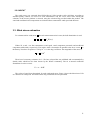
The values of a and b are determined for each wind speed range. Figure 3 shows the behaviour of CD
as a function of wind speed. The main known drag coefficients are also presented.
11
Figure 3 : comparison between various drag coefficients
3.4. Sampling
For each scatterometer swath, the data (wind speed, zonal component, meridional component, wind
strees, zonal wind stress, and meridional wind stress) are averaged in each 1° x 1° grid point in order to
reduce spatial dependency between the variables. The standard deviation and the number of observations
in each box are recorded.
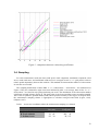
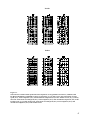
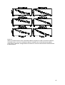
The sampling distributions of these ERS 1° x 1° scatterometer " observations " are summarized in
Figure 4. They are evaluated for eight ocean areas indicated by table 1. On average, three or four 1° x 1° "
observations " are found in each grid point during one week. The distribution of the observation number
is different in North Atlantic (Figure 4). The mean value is the lowest and then events are under-sampled.
This is due to Synthetic Aperture Radar (SAR) which operates routinely in this region. In tropical areas,
the scatterometer sampling scheme is appropriate to calculate averaged wind fields (Legler, 1991),
(Halpern, 1987).
Table 1. : Ocean area coordinates where the scatterometer sampling is evaluated
Zones
A/ North Pacific
B/ North Atlantic
C/ Indian Ocean
Lat. min.,
Lat. max.
30, 60
30, 60
-30, 30
Long. min.,
Long. max.
115, 290
290, 20
20, 115
12
D/ Tropical Pacific
E/ Tropical Atlantic
F/ South Indian Ocean
G/ South Pacific
H/ South Atlantic
-30,
-30,
-60,
-60,
-60,
30
30
-30
-30
-30
115,
290,
20,
115,
290,
290
20
115
290
20
Figure 4 : The distribution (Frequency) of the number of scatterometer overpasses per week for four 1x1 deg.
latitude-longitudeareas estimated for eigth areas (Table 1). The x-axis stands for sampling length and the y-axis
stands for the frequency
3.5. Estimation of gridded wind fields
Since wind estimated at a point can vary significantly over periods of a few hours, it is difficult to
reconstruct the synoptic fields of surface winds at basin scales from discrete observations, without the use
of an appropriate method. Thus we have developed a statistical technique for the objective analysis of
remote sensor wind data. This statistical interpolation is a minimum variance method related to the
kriging technique widely used in geophysical studies. The analysis scheme is based on determining the
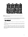
estimator of surface parameters derived from scatterometer measurements. Figure 5 shows an example of
seven days of scatterometer coverage.
The computational details in constructing a regular wind field from polar orbit satellite data are given
by Bentamy et al (1996). Briefly, let V(X) be an observation at point X=(x,y,t), where x and y are the
spatial locations and t indicates time. We suppose that V(X) is a realization of the variable <U>(X).
13
Figure 5 : One week coverage of ERS-1 scatterometer observations : number of samples in each 1° x 1° cell.
We assume that each measurement consists of the true value plus a random error :
V(X) = <U>(X)+ (X)
The analysis scheme is based on the determination of the estimator Û of <U>, at a grid point X0, of
the surface variables using N observations V at the point Xi (referred as neighbourhood) :
Here Xi stands for spatial and temporal coordinates. The weights λ are determined as the minimum of
the linear system named kriging system :
Where Γ is the structure function, named variogram. It allows the spatial and temporal variability
behavior of the variable to be estimated. It is defined as :
E() and C() indicate the statistical mean and covariance functions, respectively.
14
Furthermore, the kriging method provides an expression for variance error, named kriging variance,
which indicates the accuracy of the estimated wind variable at each grid point. The solution of the kriging
system is used to calculate the variance of the difference between the estimated value Û and the true value
<U> of the surface parameter :
In order to resolve the kriging system it is necessary to acquire the best possible knowledge of the
variogram Γ. Several models exist to define the theoretical formulation of the variogram. In the
scatterometer case, the exponential model appears suitable. Its expression in terms of space and time
separation is given by the equation :
where a, named sill value, corresponds to the variogram value when there is no correlation between
variables. b, named spatial variogram range, corresponds to the spatial lag beyond which there is no more
structure or where variables are uncorrelated. c is used to indicate the time correlation between variables.
Coefficient ε corresponds to the spatial noise on scatterometer wind vector estimates. The calculation of ε
indicates that its value is close to zero.
For instance the estimated values of variogram parameters a, b and c for scatterometer wind speed,
zonal component and meridional component in the tropical area are given by table 2.1.
For instance, table 2.1 gives the estimated values of variogram parameters a, b and c for scatterometer
wind speed, zonal component and meridional component in the tropical area.
Table 2.1 : Values of the variogram coefficients used for wind speed
Wind Speed
Zonal Component
Meridional Component
a (m2/s2)
11.3
49.8
38.1
b(km)
600.
600.
600.
c(km/hour)
30.
30.
30.
Table 2.2 : Values of the variogram coefficients used for wind stress
Wind Stress
Zonal Component
Meridional Component
a (Pa2)
0.00335
0.00395
0.00525
b(km)
600.
600.
600.
c(km/hour)
15.85
13.93
23.0
15
Figure 6
The determination of a neighbourhood containing the scatterometer data used to estimate the wind
vector (wind speed, zonal and meridional components) is a quite sensitive step. Indeed, due to highly
irregular spatial and temporal arrangement and the density of the scatterometer wind observations, the
determination of a local neighbourhood is not straightforward. In the operational method (CERSAT,
1998), the neighbourhood is determined as a successive circles centred on each grid point. The radius of
these circles correspond to the variogram parameters. the maximum number of observations in grid point
neighborhood is 20, which is a compromise between an adequate spatial and temporal sampling number
16
and time computing duration. For monthly and especially NSCAT wind fields, this criteria is not
acceptable. Indeed, NSCAT has a better spatial coverage than ERS-1/2.
Therefore, the new procedure takes into account all samples located within the neighbourhood. Their
number reaches 1200. This data set is then sorted by time and for each hour the closest scatterometer
observations from the grid point are used for wind vector estimation.
3.6. Wind divergence and stress curl estimation
The wind divergence, Div(V), and the stress curl, curl( ), at each 1° x 1° grid cell are then evaluated
from the resultant wind fields. Finite difference schemes are used to estimate the two parameters.
where
u, v are the mean zonal and meridional components of the wind vector (as estimated by kriging),
τx, τy are the mean zonal and meridional components of the wind stress vector (as estimated by
kriging),
i, j are the column and line index of the current grid cell,
dx, dy are the width and height of the current grid cell
17
4. Product description
This section describes the main characteristics of the ERS-1/ERS-2/NSCAT mean wind fields
produced at CERSAT, and provides detailed specifications of the format of the data files.
4.1. Main characteristics
4.1.1. Spatial coverage
The ERS-1/ERS-2/NSCAT mean wind fields cover global oceans from 80° North to 80° South in
latitude, and 180° West to 180° East in longitude.
4.1.2. Spatial resolution
The ERS-1/ERS-2/NSCAT mean wind fields are provided on a rectangular 1°x1° resolution grid.
4.1.3. Grid description
The data are projected on a 1° rectangular grid of 360 columns and 160 lines. A grid cell spans 1° in
longitude and 1° in latitude. Latitude and longitude of each grid cell refers to its center. The origin of
each data grid is the grid cell defined by 179.5° West in longitude and 79.5° North in latitude. The last
grid cell is centered at 79.5° South and 179.5° East.
4.1.4. Temporal coverage
Mean winds fields are available :
from 5th August 1991 to 2nd June 1996 for ERS-1
from 25th March 1996 to 15thJanuary 2001 for ERS-2
from 16th September 1996 to 30th June 1997 for NSCAT
4.1.5. Temporal resolution
Two different temporal resolutions are provided:
The weekly mean covers the time period from Monday 0h to Sunday 24h in the current week
The monthly mean covers the time period from the first day at 0h to the last day at 24h in the
current month
4.1.6. Land mask
18
The 1° resolution land mask was computed from the GMT coastline database (compiled from World
Vector Shorelines -WVS- and CIA World Data Bank -WBDII-). Inner lakes are masked.
4.1.7. Ice mask
No wind values are retrieved over polar sea-ice. The ice mask used is derived from ERS-1/ERS-2
open-ocean/sea-ice boundaries computed at CERSAT (refer to the ERS-1 & ERS-2 Polar Sea Ice Atlas
product, by R.Ezraty – more details on CERSAT web site: http://www.ifremer/cersat). The mask
edge fits approximately the 10% ice concentration limit.
4.1.8. Main parameters
Wind speed modulus: 0 – 60 m/s
Zonal wind component: -60 – 60 m/s
Meridional wind component: -30 – 30 m/s
Wind stress modulus: 0 – 2.5 Pa
Zonal wind stress component: - 2.5 – 2.5 Pa
Meridional wind stress component: - 2.5 – 2.5 Pa
Wind vector divergence: - 10-3 – 10-3 s-1
Wind stress curl: -2.5 – 2.10-5 Pa/m
The estimated error of each at the above parameters is provided with the same unit.
4.1.9. Storage
Data are currently stored as netCDF (network Common Data Form) files. Each file contains all
parameters for a given date and time resolution (week or month) using the following naming
convention:
<Start date>-<End date>.nc with dates as ‘YYYYMMDDhhmm’
ex: 200010010000-200010020000.nc (daily mean from 1st October to 2nd October 2000)
200010010000-200011010000.nc (monthly mean, October 2000)
Further information about netCDF format
http://www.unidata.ucar.edu/packages/netcdf/
can
be
found
on
UCAR
web
site
:
4.1.10. Data volume
About 1.8 Mo for each file (500 Ko when zipped).
4.1.11. Conventions
Times are UTC.
The longitude reference is the Greenwich meridian: longitude is positive eastward, negative westward
and ranges between [-180, 180[ (compatibility within the WOCE package).
The latitude reference is the Equator: latitude is positive in the northern hemisphere, and negative in
the southern hemisphere.
19
4.2. Header structure
Element name
WOCE_version
CONVENTIONS
long_name
Type
String
String
string
short_name
string
producer_agency
producer_institution
netcdf_version_id
product_version
creation_time
start_date
stop_date
time_resolution
string
string
string
string
string
string
string
string
spatial_resolution
platform_id
instrument
objective_method
south_latitude
north_latitude
west_longitude
east_longitude
string
string
string
string
float
float
float
float
Format
3.0
"COARDS/WOCE"
‘<scatterometer> <period> mean wind fields’
scatterometer ∈ {ERS-1, ERS-2, NSCAT}
period ∈ { weekly, monthly}
‘MWF-<scatterometer>-<period>’
scatterometer ∈ {E1, E2, N}
period ∈ {D,W,M}
‘IFREMER’
‘CERSAT’
‘3.4’
‘1.0’
‘YYYY-DDDTHH:MM:SS.SSS’
‘YYYY-DDDTHH:MM:SS.SSS’
‘YYYY-DDDTHH:MM:SS.SSS’
‘<T>’
T∈ { one week mean, one month mean}
‘1 degree’
{‘ERS-1’, ‘ERS-2’, ‘ADEOS’}
{‘AMI-Wind’, ‘NSCAT’
‘kriging’
+/-xx.yyyy [-90, 90]
+/-xx.yyyy [-90, 90]
xxx.yyyy [ -180, 180[
xxx.yyyy [ -180, 180[
4.2.1. WOCE_version
The mean wind fields are part of WOCE package. The current WOCE version is "3.0".
4.2.2. CONVENTIONS
The netCDF standard conventions which the product conforms to. The convention is always
"COARDS" that means Cooperative Ocean/Atmosphere Research Data Service. The information on
the standard can be found at http://ferret.wrc.noaa.gov/noaa_coop/coop_cdf_profile.html. Some
additional WOCE rules extend this convention.
4.2.3. long_name
A complete descriptive name for the product. The long_name has the format ‘sensor period mean
wind fields’ where sensor is the instrument or satellite (‘ERS-1’, ‘ERS-2’ and ‘NSCAT’) which
collected the raw data averaged on the grid and period is the time interval over which raw data are
averaged (‘daily’, ‘weekly’, ‘monthly’).
4.2.4. short_name
The official reference of the product. The format is ‘MWF-sensor_id-period_id’ where sensor_id
(‘E1’ for ERS-1, ‘E2’ for ERS-2, ‘N’ for NSCAT) is the identifier of the sensor used and period_id is
20
the identifier of the time interval over which raw data are averaged (‘D’ for daily means, ‘W’ for
weekly means, ‘M’ for monthly means).
4.2.5. producer_agency
The agency that provides the project funding. The nominal value is ‘IFREMER’.
4.2.6. producer_institution
The institution (here department) that provides project management. The nominal value is ‘CERSAT’.
4.2.7. netcdf_version_id
A character string, which identifies the version of the netcdf (Network Common Data Form) library,
which was used to generate this data file. The netcdf libraries are developed by Unidata Program
Centre in Boulder, Colorado.
4.2.8. product_version
A character string, which identifies the version of the software, used to generate this data file. The
format of this string is x.y where x.y the release identification number.
4.2.9. creation_time
The clock time when the data file was produced. The format of the date is YYYY-DDDTHH:MM:SS
where YYYY is the calendar year, DDD the day of the year, HH represents the hour in twenty four hour
time, MM the minutes and SS the seconds.
4.2.10. start_date
The UTC start date of the time interval over which the raw data are averaged on the grid. The format
of the date is YYYY-DDDTHH:MM:SS where YYYY is the calendar year, DDD the day of the year, HH
represents the hour in twenty four hour time, MM the minutes and SS the seconds.
4.2.11. stop_date
The UTC end date of the time interval over which the raw data are averaged on the grid. The format of
the date is YYYY-DDDTHH:MM:SS where YYYY is the calendar year, DDD the day of the year, HH
represents the hour in twenty four hour time, MM the minutes and SS the seconds.
4.2.12. time_resolution
The length of the time interval over which the raw data are averaged on the grid. The nominal values
are ‘one week mean’ for the weekly means and ‘one month mean’ for the monthly means.
4.2.13. spatial_resolution
21
The size -in latitude and longitude- of the cells of the product grids. The nominal value is ‘1 degree’.
4.2.14. platform_id
The identifier (name) of the satellite on which the wind sensor (scatterometer) is embedded. ‘ERS-1’,
‘ERS-2’ or ‘ADEOS-1’.
4.2.15. instrument
The identifier (name) of the scatterometer collecting the raw wind values averaged on the grids. ‘AMIWind’ or ‘NSCAT’.
4.2.16. objective_method
The objective method used to average the raw wind values and fill the gaps on the grid. The nominal
value is ‘kriging’.
4.2.17. north_latitude
The north latitude of the rectangular grid on which the wind values are averaged. The latitude
reference is the Equator : latitude is positive in the northern hemisphere, and negative in the southern
hemisphere. The nominal value is 80.00.
4.2.18. south_latitude
The south latitude of the rectangular grid on which the wind values are averaged. The latitude
reference is the Equator : latitude is positive in the northern hemisphere, and negative in the southern
hemisphere. The nominal value is -80.00.
4.2.19.west_longitude
The west longitude of the rectangular grid on which the wind values are averaged. The longitude
reference is the Greenwich meridian : longitude is positive eastward, negative westward and ranges
between [-180, 180[ (compatibility within the WOCE package). The nominal value is -180.00.
4.2.20.east_longitude
The east longitude of the rectangular grid on which the wind values are averaged. The longitude
reference is the Greenwich meridian : longitude is positive eastward, negative westward and ranges
between [-180, 180[ (compatibility within the WOCE package). The nominal value is -180.00.
4.3. Data structure
22
Element name
time
depth
woce_date
woce_time
latitude
longitude
swath_count
quality_flag
wind_speed
wind_speed_error
zonal_wind_speed
zonal_wind_speed_error
meridional_wind_speed
meridional_wind_speed_error
wind_speed_divergence
wind_stress
wind_stress_error
zonal_wind_stress
zonal_wind_stress_error
meridional_wind_stress
meridional_wind_stress_error
wind_stress_curl
conceptual type
Integer
Real
string
time
real
real
integer
integer
real
real
real
real
real
real
real
real
real
real
real
real
real
real
storage type
Int
Float
int
float
float
float
short
byte
short
short
short
short
short
short
short
short
short
short
short
short
short
short
dimensions
[1]
[1]
[1]
[1]
[160]
[360]
[160, 360]
[160, 360]
[160, 360]
[160, 360]
[160, 360]
[160, 360]
[160, 360]
[160, 360]
[160, 360]
[160, 360]
[160, 360]
[160, 360]
[160, 360]
[160, 360]
[160, 360]
[160, 360]
units
Hours
m
UTC
UTC
degrees_north
degrees_east
scale_factor
1
1
valid_min
valid_max
10
10
1
1
-80
-180.
80
179,99
m/s
m/s
m/s
m/s
m/s
m/s
s-1
Pa
Pa
Pa
Pa
Pa
Pa
Pa/m
0.01
0.01
0.01
0.01
0.01
0.01
10-7
0.001
0.001
0.001
0.001
0.001
0.001
10-9
0.
0.
-60.
0.
-60.
0.
-10-3
0.
0.
-2.5
0.
-2.5
0.
-2.10-5
60.
10.
60.
10.
60.
10.
10-3
2.5
1.
2.5
1.
2.5
1.
2.10-5
23
4.3.1. time
This parameter indicated the number of hours passed since 1900-1-1 0:0:0.This parameter is
included for compatibility within the WOCE package.
Conceptual type
Storage type
Number of bytes
Units
Minimum value
Maximum value
integer
Int32
4
hours
First hour of this file period
Last hour of this file period
4.3.2. depth
This parameter indicates the depth of the measurement. Scatterometer surface wind estimates
are calculated at 10m height in neutral condition. Therefore the depth parameter is set to +10
(the sea surface has the depth 0, and the positive depth are above the sea surface). This
parameter is included for compatibility within the WOCE package.
Conceptual type
Storage type
Number of bytes
Units
Minimum value
Maximum value
real
float
4
meters
10
10
4.3.3. woce_date
This parameter indicates the date of the averaged period. The value refers to the centre of the
time period, in UTC, using the YYYYMMDD format. The start_date and stop_date attributes of
the woce_date variable indicate the beginning and the end of this period using the same format.
The time_interval attribute indicates the time resolution of the averaged period (‘one day’, ‘one
week’ or ‘one month’). This parameter is included for compatibility within the WOCE package
and is fully redundant with start_date and stop_date global attributes.
Conceptual type
Storage type
Number of bytes
Units
Start date
Stop date
Time interval
string
Int32
4
UTC
YYYYMMDD
YYYYMMDD
‘one
4.3.4. woce_time
This parameter indicates the time of the averaged period. The value refers to the centre of the
time period, in UTC, using the hhmmss.dd format. The start_time and stop_time attributes of the
woce_time variable indicate the beginning and the end of this period using the same format.
This parameter is included for compatibility within the WOCE package and is fully redundant
with start_date and stop_date global attributes.
Conceptual type
Storage type
Number of bytes
Units
Start time
Stop time
real
float
4
UTC
hhmmss.dd
hhmmss.dd
23
4.3.5. latitude
This parameter indicates the latitude corresponding to a given grid row. The latitude value refers
to the centre of the cells of this row. The latitude reference is the Equator: latitude is positive in
the northern hemisphere, and negative in the southern hemisphere.
Conceptual type
Storage type
Number of bytes
Units
Minimum value
Maximum value
Scale factor
real
float
4
degree
-80
80
1.
4.3.6. longitude
This parameter indicates the longitude corresponding to a given grid column. The longitude
value refers to the centre of the cells of this column. The longitude reference is the Greenwich
meridian: longitude is positive eastward, negative westward and ranges between [-180, 180[
(compatibility within the WOCE package).
Conceptual type
Storage type
Number of bytes
Units
Minimum value
Maximum value
Scale factor
real
float
4
degree
-180.00
179.99
1.
4.3.7. swath_count
This parameter indicates the number of averaged scatterometer swaths over a given grid cell.
Conceptual type
Storage type
Number of bytes
Units
Minimum value
Maximum value
Scale factor
integer
Int 16
2
count
0
32767
1
4.3.8. quality_flag
This flag indicates the quality of the mean wind computation over a given grid cell. The
significance of each flag value is as follow:
Bit
0
1
2
Definition
Ice detection
0 : no ice detected
1 : sea ice detected within the grid cell. No mean wind was computed
Land detection
0 : no land detected
1 : land detected within the grid cell. No mean wind was computed
Mean wind retrieval
0 : mean wind was correctly retrieved
1 : mean wind was not computed because of too low sampling
24
3
4
5
Mean stress retrieval
0 : mean stress was correctly retrieved
1 : mean stress was not computed because of too low sampling
Mean wind in valid range
0 : mean wind was reported in valid range
1 : mean wind was out of valid range
Mean stress in valid range
0 : mean stress was reported in valid range
1 : mean stress was out of valid range
Conceptual type
Storage type
Number of bytes
Units
Minimum value
Maximum value
Scale factor
enum
int8
1
n/a
0
255
1
4.3.9. wind_speed
The mean wind speed of the surface wind vector computed within a given grid cell, using the
kriging method.
Conceptual type
Storage type
Number of bytes
Units
Minimum value
Maximum value
Scale factor
real
int16
2
m/s
0.0
60.0
0.01
4.3.10. wind_speed_error
The wind speed error of the surface wind vector computed within a given grid cell, using the
kriging method. This parameter indicates the quality of the estimator; for high values, which
correspond to sampling problems, low wind speed or high variability, the gridded data should
be used carefully.
Conceptual type
Storage type
Number of bytes
Units
Minimum value
Maximum value
Scale factor
real
int16
2
m/s
0
10.0
0.01
4.3.11. zonal_wind_speed
The mean zonal wind vector component computed within a given grid cell, using the kriging
method. The zonal wind component is positive for eastward wind direction.
Conceptual type
Storage type
Number of bytes
Units
Minimum value
real
int16
2
m/s
-60.00
25
Maximum value
Scale factor
60.00
0.01
4.3.12. zonal_wind_speed_error
The mean zonal wind vector component error computed within a given grid cell, using the
kriging method. This parameter indicates the quality of the estimator; for high values, which
correspond to sampling problems, low wind speed or high variability, the gridded data should
be used carefully.
Conceptual type
Storage type
Number of bytes
Units
Minimum value
Maximum value
Scale factor
real
int16
2
m/s
0.00
10.00
0.01
4.3.13. meridional _wind_speed
The mean meridional wind vector component computed within a given grid cell, using the
kriging method. The meridional wind component is positive for northward wind direction.
Conceptual type
Storage type
Number of bytes
Units
Minimum value
Maximum value
Scale factor
real
int16
2
m/s
-60.00
60.00
0.01
4.3.14. meridional_wind_speed_error
The mean meridional wind vector component error computed within a given grid cell, using the
kriging method. This parameter indicates the quality of the estimator; for high values, which
correspond to sampling problems, low wind speed or high variability, the gridded data should
be used carefully.
Conceptual type
Storage type
Number of bytes
Units
Minimum value
Maximum value
Scale factor
real
int16
2
m/s
0.00
10.00
0.01
4.3.15. wind_speed_divergence
The divergence of the wind vector, computed from the mean wind vector grids using the second
order finite difference scheme.
Conceptual type
Storage type
Number of bytes
Units
real
int16
2
s-1
26
Minimum value
Maximum value
Scale factor
-10-3
10-3
-10-7
4.3.16. wind_stress
The mean surface wind stress magnitude, computed within a given grid cell, uses the kriging
method. The wind stress individual measurements used in averaging were calculated from the
raw wind values using the Smith (1988) bulk formulation.
Conceptual type
Storage type
Number of bytes
Units
Minimum value
Maximum value
Scale factor
real
int16
2
Pa
0.0
2.5
0.001
4.3.17. wind_stress_error
The mean error of the surface wind stress magnitude, computed within a given grid cell, using
the kriging method. This parameter indicates the quality of the estimator; for high values, which
correspond to sampling problems, low wind stress or high variability, the gridded data should be
used carefully.
Conceptual type
Storage type
Number of bytes
Units
Minimum value
Maximum value
Scale factor
real
int16
2
Pa
0.0
1.0
0.001
4.3.18. zonal_wind_stress
The mean zonal surface wind stress component, computed within a given grid cell, uses the
kriging method. The wind stress individual measurements used in averaging were calculated
from the raw wind values using the Smith (1988) bulk formulation.
Conceptual type
Storage type
Number of bytes
Units
Minimum value
Maximum value
Scale factor
real
int16
2
Pa
-2.5
2.5
0.001
4.3.19. zonal_wind_stress_error
The mean error of the zonal surface wind stress component, computed within a given grid cell,
using the kriging method. This parameter indicates the quality of the estimator; for high values,
which correspond to sampling problems, low wind stress or high variability, the gridded data
should be used carefully.
27
Conceptual type
Storage type
Number of bytes
Units
Minimum value
Maximum value
Scale factor
real
int16
2
Pa
0.0
1.0
0.001
4.3.20. meridional_wind_stress
The mean meridional surface wind stress component, computed within a given grid cell, uses
the kriging method. The wind stress individual measurements used in averaging were calculated
from the raw wind values using the Smith (1988) bulk formulation.
Conceptual type
Storage type
Number of bytes
Units
Minimum value
Maximum value
Scale factor
real
int16
2
Pa
-2.5
2.5
0.001
4.3.21. meridional_wind_stress_error
The mean error of the meridional surface wind stress component, computed within a given grid
cell, using the kriging method. This parameter indicates the quality of the estimator; for high
values, which correspond to sampling problems, low wind stress or high variability, the gridded
data should be used carefully.
Conceptual type
Storage type
Number of bytes
Units
Minimum value
Maximum value
Scale factor
real
int16
2
Pa
0.0
1.0
0.001
4.3.22. wind_stress_curl
The curl of the wind stress vector, computed from the mean wind stress vector grids using the
second order finite difference scheme.
Conceptual type
Storage type
Number of bytes
Units
Minimum value
Maximum value
Scale factor
real
int16
2
Pa/m
-2.10-5
2.10-5
10-9
28
5. Data use
5.1. Data access
5.1.1. Ftp access
All mean wind fields (MWF) data files, continually updated, can be downloaded through
anonymous ftp at IFREMER/CERSAT:
ftp://ftp.ifremer.fr/ifremer/cersat/products/gridded/
5.1.2. WWW access
The data can be subsetted on time and space criteria on CERSAT web site:
http://www.ifremer.fr/cersat
Go to ‘Data’ then ‘Extraction’
5.1.3. On-line browser
All fields can be browsed on CERSAT web site:
http://www.ifremer.fr/cersat
Go to ‘Data’ then ‘Quicklook’
5.2. Reading the data
The data produced are stored under the netCDF standard interface for array oriented data access
and provides freely distributed libraries for C, Fortran, C++, Java and perl that provide
implementation
of
the
interface.
Further information can
be
found
at
http://www.unidata.ucar.edu/packages/netcdf/guide.txn_doc.html
29
6. Validation & accuracy
6.1.Accuracy of scatterometer winds
The accuracies of ERS and NSCAT retrieval wind speed and direction were determined
through a comparisons with buoy wind measurements (Quilfen et al, 1994; Graber et al, 1996;
Graber et al, 1997). Three buoy networks were used to estimate the quality of the retrieved
scatterometer wind vectors (Figure 7) : the National Data Buoy Center (NDBC) buoys-off the U.S.
Atlantic, Pacific and Gulf coasts maintained by the National Oceanic and Atmospheric
Administration (NOAA); the Tropical Atmosphere Ocean (TAO) buoys located in tropical Pacific
Ocean and maintained by the NOAA Pacific Marine Environmental Laboratory (PMEL); and the
European buoys-off European coasts called ODAS and maintained by U.K. Met office and MeteoFrance.
NDBC buoys have a propeller-vane anemometer recorded once every hour an 8-min average of
the wind speed and a single direction with accuracies of 1m/s and 10°, respectively (Gilhousen,
1987). The height of NDBC anemometer used in this study is about 5m. TAO buoy measured
winds at 3.8m height using a propeller-vane anemometer. The wind speed and direction are both
sampled at 2 Hz and recorded for 1 hour vector-averaged east-west and north-south components
(Hayes et al, 1991). Finaly, the ODAS buoy wind measurements are made in the northeast Atlantic.
The wind speed and wind direction are measued by a cup anemometer and windvane ,
respectivelly. Both measurements are made at 4m height and recorded once every hour 10-min
average (see http://mozart.shom.fr/meteo/index-fr.html). Only ODAS measurements recorded
during NSCAT period are used in this sutudy. the calculation of buoy wind speed at 10m height in
neutral condition is performed using LKB model (Liu et al, 1979). For the three networks, only
hourly buoy wind speed and direction estimates are used in the scatterometer/buoy wind
comparisons.
For instance, the results obtained by Graber et al (1996) indicated that the ERS-1 scatterometer
wind speeds are biased lower according to buoy winds. The bias values derived from ERS1/NDBC, and from ERS-1/TAO comparisons are 0.30m/s and 1m/s, respectively. The
corresponding rms values are 1.13m/s and 1.38m/s. The comparisons between wind direction
retrieved from ERS-1 scatterometer and measured by buoys provided a rms error of 24° for both
buoy networks. Using similar collocation procedures, Graber et al (1997), showed that the
difference between NDBC and NSCAT wind speeds has a mean and rms values of 0.14m/s and
1.22m/s, respectively. For the NSCAT wind direction, the rms error is about 24° . The results
inferred from NSCAT/TAO comparisons (Caruso et al, 1999), indicated that for wind speed, the
bias is very low, and the rms difference is about 1.55m/s, and for wind direction, the rms difference
is about 20°. The results obtained from ERS-2 scatterometer / buoy comparisons are quite similar
to those obtained for ERS-1. However, it was found that the overall bias of ERS-2 scatterometer
wind speed is higher than ERS-1 one, with respect to scatterometer/buoy comparisons (Quilfen et
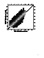
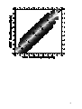
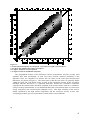
al, 1999). Figure 8 shows scatter-plots of comparison of ERS-2 and NSCAT wind speeds with
buoy winds at 10-m for NDBC, TAO and ODAS buoys. Most of statistical parameters, provided
within each figure, are quite similar to those obtained from previous studies and cited above.
However, the bias on ERS-2 wind speed is significant and requires correction.
To enhance the statistical quality of the retrieved ERS-1/2 scatterometer wind speed, a
collocated data set between ERS-1/2 and NDBC buoy measurements was made up. All ERS-1/2
scatterometer valid measurements performed within one hour and 50km from buoy measurement
wind measurements during the period March 1992 - November 1998 were selected. The collocated
data set was then used to derive a new version of ERS C-band model (Bentamy et al, 1994). The
latter is used to retrieve ERS-1/2 scatterometer wind speed observations from measured backscatter
30
coefficients. Hence, the ERS-1/2 gridded wind fields are calculated from the ERS-1/2 corrected
wind speeds and from the ERS-1/2 standard wind directions.
Figure 7
Figure 8
31
6.2. Aliasing in regular wind fields
As indicated in section 2, the width of a ERS-1 and NSCAT scatterometer swaths are 500km,
and two times 600 km, respectively. Their orbits are about 101 mn. Hence, scatterometer wind
estimates could be close in space but widely separated in time. In some regions, such as the North
Atlantic, wind variability at a given location could be high during a period of a few hours. Even
though the kriging method uses a structure function of wind variables, it is necessary to investigate
the impact of the number and of the spatial and temporal distribution of the observations used to
estimate wind at each grid point. This involves the impact of scatterometer sampling on the
accuracy of the method and also how the objective method restitutes highly variable events.
The best way to check the aliasing problem is to simulate scatterometer wind sampling from
regular surface wind, considered as the "ground truth", and then to compare the resultant wind field
with the initial one. The European Center for Medium-Range Weather Forecasts (ECMWF) surface
wind analysis is used. The spatial resolution of ECMWF analysis is 1.125 x 1.125 deg in longitude
and latitude. The analysis is provided at synoptic time (00h, 06h, 12h, 18h). At each scatterometer
cell, ECMWF wind data are linearly interpolated in time and space. This simulated scatterometer
data, indicated hereafter by Simu_Scat, is used to generate a regular wind field using the kriging
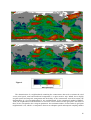
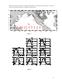
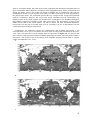
approach. An example of two weekly wind fields calculated from ECMWF analysis, used as wind
field control, and from Simu_Scat wind data is shown in Figures 9a and 9b, respectively. The
averaging period is a week in December, when the wind is highly variable in the Northern
hemisphere. The comparison between the fields is quite good. They exhibit similar large wind
structures. The deviation of Simu_scat wind speed from ECMWF analysis is shown in Figure 9c.
One result is that the kriging approach does not provide any large banded structure due to polar
scatterometer sampling.
The analysis of the scatterplot comparison between true and simulated weekly wind fields does
not exhibit any systematic error in the wind estimates (not shown). In general speaking, the
difference between the two fields varies between -1.5m/s and 1.5m/s (in term of zonal component).
However, some high values are found and correspond to the regions where wind variability is high
and/or the scatterometer sampling number is poor (Bentamy et al, 1998). For instance, in the
extratropical northern latitudes difference values exceeding 2m/s are observed. In such regions, the
standard deviation of ECMWF zonal wind component is six times higher than in the region where
difference between true and simulated scatterometer gridded wind fields are low. It is not
surprising that NSCAT sampling scheme cures significantly to such problems compared to gridded
wind fields estimated from ERS-1/2. The correlation values, estimated at equator, between
simulated and true variables are about 98% for ERS-2, and 99% for NSCAT. In southern ocean, the
correlation drops to 97% for ERS-2, while for NSCAT it remains great than 98%.
Similar investigations were performed for monthly gridded wind fields. As expected the
differences reduce drastically with respect to weekly wind field estimates. The highest values of the
difference between true and simulated zonal component do not exceed 2.20m/s. The percentage of
grid points, with respect to total grid point number, where the difference between ECMWF and
simulated scatterometer zonal components exceeds 1.20m/s, account for 4 % for ERS-2, and 1%
for NSCAT simulations. Most of these high difference values are found in high latitudes.
32
Mean m/s
σDm/s
ECMWF-ERS-2
0.09
0.96
0.19
ECMWF-NSCAT
0.04
0.50
0.10
ECMWF-ERS
0.04
0.59
0.13
ECMWF-NSCAT
0.04
0.38
0.08
Table 3 :
ε
Weekly wind fields
Monthly wind fields
Table 1, summarizes the main statistical parameters, characterizing scatterometer sampling
impact on gridded wind field calculations. σD states for standard deviation of wind field difference.
ε is the ratio σD/σE, where σE is the standard deviation of ECMWF weekly wind field. The gridded
wind fields estimated from simulated are unbiased according to ECMWF mean wind field. The
highest value of the standard deviation σD, characterizing the deviation of weekly simulated wind
fields from ECMWF mean wind field, does not exceed 1 m/s. However,we can notice that 19 % for
ERS case, and 10 % for NSCAT case, of the standard deviation values are mainly du to the
scatterometer sampling. The use of merging simulated ERS-2 and NSCAT data reduces slightly ε
to 9 %. The calculation of zonal mean of ε indicates that its minimum values are obtained in the
tropical oceans (20° S - 20° N) : 15 % for ERS-2 and 8.5 % for NSCAT.
For monthly wind fields, we can notice that ε value reduces to 13 %, 8 % and 6 % for ERS-2,
NSCAT, and ERS-2 + NSCAT, respectivelly. The calculations of zonal mean of ε ratio indicates
that its values are quite similar over the global ocean.
Figure 9a
33
Figure 9b
Figure 9c
Figure 8 :
a/ Weekly averaged wind field computed from simulated scatterometer wind observations
b/ Weekly averaged wind field computed from ECMWF analysis
c/ Difference between ECMWF and simulated scatterometer wind fields
34
6.3. Comparison with buoy data
The aim of this section is to estimate the accuracy of the weekly and monthly wind speed and
direction in comparison with buoy wind data. This is achieved by using : the National Data Buoy
Center (NDBC), the Tropical Atmosphere Ocean (TAO), and the European Buoys (ODAS) buoy
networks (Figure 10). More than 90 buoys covering Atlantic and Pacific ocean areas between 10°S
and 57°N.
Figure 10 : Buoy network location
For the validation of the scatterometer average wind field, the buoy wind data are referenced to
10m height, assuming a logarithm wind profile, Von Karman's constant of 0.4, neutral stratification
and, a wind speed dependent drag coefficient (Ezraty 1987).
For each week and each month, mean values of buoy wind speed, zonal and meridional
components are computed arithmetically. Weekly and monthly means are computed for all ERS-1,
ERS-2 and NSCAT periods for which at least 3.5 days and 15 days buoy measurements are
collected, respectively. For each averaging period, the closest scatterometer grid point (1° x 1° ) to
each buoy location is selected. Therefore, a collocated data sets between scatterometer gridded
wind fields (averaging objective method) and buoy averaged winds are performed for NDBC, TAO
and ODAS buoy networks. Results are then compared using the following standard statistic data
analysis :
The wind speed, zonal component and meridional component are assumed as a random
variables wich could be characterized by their moments. For this purpose, the four conventional (C
moments) and linear moments (L moments) of each variable are estimated.
Let is W a wind variable (wind speed, zonal component, meridional component or wind
difference). The corresponding four C moments are determined as :
35
(4)
W , σW,
SW and KW are the W mean (bias), standard deviation, skweness and kurtosis,
respectively. Variance and rms values are derived from
W and σW estimates.
The L moments (Hosking, 1990} are defined by :
(5)
λn is the nth linear moment of W
Pl n* is the shifted nth Legendre polynomial. It is related to Legendre polynomial Pln by :
(6)
F is the probability function of wind variable W
Q(F), called quantile function, is provided by the following equation :
(7)
The meaning of C moments and L moment are similar as can be shown through the equations.
The main advantage of L moments is their relative small sensitivity to data errors generaly
producing outliers in data series.
The statistical significance of the first and second moment is evaluated by Student test (T-test)
and Fisher test (F-Test), respectively. Throughout this paper, the significance is estimated for 95%
confidence.
Moreover, the linear regression parameters are estimated to assess the comparisons between
satellite gridded wind fields and buoy averaged winds. In this paper we provide the following
parameters :
36
(8)
Where
x and y denote the buoy and scatterometer wind estimates, respectively. b is the slope and a is
the intercept on the y axis : y = bx + a. bs is the slope of symmetric regression line. ρ is the
correlation coefficient. Its calculation involves the residual, ε, between y and linear regression
model. σp1, and σp2 are the rms deviations of the first and second principal component of x and y
distribution. They provide a measurement of the major and minor axis of the elliptical x and y
distribution.
6.4. Global comparisons
Table 2, 3, and 4 provide the main statistical parameters characterizing wind speed
comparisons. The wind speed correlation coefficients ranging from 0.85 to 0.89 indicate a good
consistency between satellite and buoy averaged winds. The rms values of the differences buoysatellite wind speeds do not exceed 1.16m/s over NDBC and TAO networks. Results derived from
ODAS/satellite comparisons show higher rms values : 1.48m/s for NSCAT, and 1.66m/s for ERS2. The latter are mainly due to a poor number of comparison data points, and to the high wind
variability in ODAS area (Figure 11). Furthermore, the statistics calculated by several
meteorological centers (ECMWF, CMM, UKMet) indicate that ODAS buoy wind speed tend to be
underestimated according to meteorological wind analysis (see ftp://ftp.shom.fr/meteo/qc-stats, site
maintained by P. Blouch).
The results of the regression analyses carried out on collocated data, show that the slopes
calculated over each buoy network and against buoy wind estimates, are quite similar for the three
averaged scatterometer wind speeds. In NDBC area (Table 4), buoy and scatterometer wind speeds
agree quite closely, which is expressed by slopes of about 1 and intercepts of about zero.
Comparisons between buoy and scatterometer winds in Pacific tropical ocean give regression line
slopes of about 0.80, suggesting an overestimation of low wind speed and underestimation of high
wind speed by scatterometer wind fields compared to TAO winds. In north Atlantic area, the slopes
are very close to 1, whereas the intercepts are of about 0.50, indicating that the scatterometer wind
fields are consistently high compared to ODAS week-averaged wind speeds. The calculation of the
statistical parameters according to the buoy wind speed ranges, show that their values are made
variable by the outlying points at low and high wind speeds.
37
For the wind direction, no systematic bias is found, and the overall bias and standard deviation
about the mean angular difference are less 8° and 38° , respectively. These results are consistent
with the calibration/validation of the scatterometers against buoy (Graber et al, 1996 and 1997;
Caruso et al, 1999). For instance, in Pacific tropical area, where the wind direction is quite steady,
the standard deviation calculated for buoy wind speed higher than 5m/s, does not exceed 17° .
Table 4 : Comparison of averaged weekly wind speed and direction estimated from NDBC buoy
measurements and from ERS-1, ERS-2 and NSCAT scatterometer observations.
Data
SET
BuoyWind Length Wind Speed (m/s)
Speed
Range(m/s)
Bias Rms r
(m/s) (m/s)
NDBC/
ERS-1
NDBC/
ERS-2
NDBC/
NSCAT
Wind
Direction
b
a
bs
s p1
s p2
Bias Std
(deg) (deg)
0-24
3281
0.02
1.16
0.88 0.99 0.00
1.16 2.87 0.78
3
35
0-5
320
-0.14 1.03
0.74 0.87 0.68
2.12 1.14 0.47
5
47
5-10
2603
0.05
1.16
0.83 1.01 -0.14 1.35 2.04 0.72
3
34
> 10
358
-0.0
1.31
0.76 0.97 0.32
1.80 1.64 0.69
3
30
0-24
1921
0.35
1.15
0.89 0.96 -0.07 1.12 2.76 0.75
6
33
0-5
142
0.06
0.82
0.75 0.87 0.50
1.85 0.96 0.42
0
47
5-10
1581
0.37
1.16
0.83 0.98 -0.23 1.30 1.97 0.71
6
33
> 10
198
0.40
1.26
0.77 0.82 1.61
1.42 1.60 0.75
6
25
0-24
522
-0.38 1.02
0.90 0.96 0.68
1.09 2.58 0.65
8
25
0-5
28
-0.54 0.94
0.76 1.08 0.17
1.95 0.95 0.37
3
29
5-10
444
-0.37 1.01
0.85 0.96 0.69
1.21 1.87 0.62
8
26
> 10
50
-0.32 1.15
0.79 0.78 2.68
1.24 1.62 0.74
7
15
Table 5 : Comparison of averaged weekly wind speed and direction estimated from TAO buoy
measurements and from ERS-1, ERS-2 and NSCAT scatterometer observations.
Data
SET
TAO /
ERS-1
BuoyWind Length Wind Speed (m/s)
Speed
Range(m/s)
Bias
(m/s)
Rms
(m/s)
r
Wind
Direction
b
a
bs
s p1
s p2
Bias
(deg)
Std
(deg)
0-24
10047
0.29
0.89
0.89 0.80 0.85
0.94 2.15 0.59
3
31
0-5
3262
-0.14
0.85
0.76 0.70 1.31
1.32 1.06 0.54
1
51
5-10
6693
0.47
0.91
0.84 0.86 0.42
1.12 1.51 0.54
5
17
38
TAO /
ERS-2
TAO /
NSCAT
> 10
92
0.24
0.92
0.70 0.24 7.66
2.69 0.86 0.31
8
9
0-24
6737
0.56
1.03
0.89 0.80 0.63
0.93 2.26 0.60
3
27
0-5
1925
0.06
0.84
0.75 0.67 1.22
1.35 1.01 0.54
4
45
5-10
4736
0.75
1.10
0.85 0.87 0.12
1.11 1.60 0.55
5
16
> 10
76
0.76
1.14
0.78 1.74 -8.48
2.94 1.02 0.26
7
10
0-24
1780
-0.26
0.92
0.88 0.80 1.47
0.94 2.20 0.62
5
20
0-5
515
-0.70
1.18
0.74 0.71 1.81
1.61 1.10 0.55
2
33
5-10
1246
-0.08
0.79
0.83 0.80 1.39
1.07 1.47 0.55
7
11
> 10
19
0.03
0.82
0.78 1.85 -8.92
3.09 0.99 0.24
10
5
Table 6 : Comparison of averaged weekly wind speed and direction estimated from ODAS buoy
measurements and from ERS-2 and NSCAT scatterometer observations
Data
SET
BuoyWind Length
Speed
Range(m/s)
Wind Speed (m/s)
Wind
Direction
Bias
(m/s)
Rms
(m/s)
r
b
a
222
-0.70
1.66
0.88 1.02 0.51
0-5
10
-1.26
2.01
5-10
155
-0.61
> 10
57
bs
Bias
(deg)
Std
(deg)
1.20 3.58 0.99
1
38
0.72 0.63 2.65
1.96 1.65 0.76
31
75
1.68
0.80 1.18 -0.76
1.73 2.31 0.82
3
39
-0.83
1.50
0.80 0.78 3.31
1.20 1.91 0.85
4
22
194
-0.63
1.48
0.91 1.00 0.55
1.13 3.82 0.91
2
30
0-5
6
-1.29
2.07
0.72 0.51 3.26
1.96 1.65 0.79
14
76
5-10
118
-0.62
1.44
0.81 1.12 -0.37
1.58 2.05 0.73
1
30
> 10
70
-0.57
1.47
0.86 1.11 -0.84
1.37 2.73 0.82
9
22
ODAS 0-24
/ ERS-2
ODAS/ 0-24
NSCAT
s p1
s p2
39
40
41
42
Figure 11 :
a/ Scatter plot and frequency of wind speeds, x-axis shows averaged TAO wind speed,
y-axis shows the gridded scatterometer wind speed
b/ as Figure 12a but for zonal component
c/ as Figure 12a but for meridional component
The geographical features of the difference between scatterometer and buoy weekly wind
estimates have been investigated. At each TAO buoy location, statistical parameters of the
difference series are computed. For instance the rms values of the wind speed and direction
differences are shown in Figure 11. The main result is that the rms values are generally higher
within the 150E and 170E Pacific band. A study of the correlation between in-situ and sensor
matchups indicates that there is a significant difference between the correlation coefficients
computed in the eastern Pacific and those computed in the western Pacific with 95 % confidence.
Using TAO buoy measurements, it was determined that in the western Pacific there is 6 times more
energy compared to the eastern Pacific (Mangum, 1992) . This high variability of the wind is
mainly explained by the high surface temperature and the convective activity of this zone.
Averaging procedures give less representative results in these wind conditions.
a)
43
1.00
9N
1.04
8N
5N
1.13
0.87
0.81
0.92
0.89
1.09
1.19
2N
0.92 1.09
1.03
0.85
0.86
0.85
0N
0.86
0.75
0.87
0.80
0.76
2S
0.97
0.83
0.86
0.77
0.89
5S
0.77
0.68
0.80
0.89
0.73
0.89
8S
0.95
1.07
1.16
0.88
0.92
1.16
1.06
0.84
1.02
1.03
95W 110W 125W 140W 155W 170W 170E 165E 156E 154E 147E 143E 137E
b)
36
9N
33
8N
5N
40
24
17
26
31
54
62
2 N 34
33
19
14
22
28
0N
26
28
22
19
33
2S
27
21
23
18
25
5S
20
19
22
28
8S
23
52
39
54
76
62
63
62
55
73
63
42
95W 110W 125W 140W 155W 170W 170E 165E 156E 154E 147E 143E 137E
Figure 11 :
a/ Geographical behavior of the rms difference between gridded scatterometer and averaged TAO wind speeds
b/ Geographical behavior of the rms difference between gridded scatterometer and averaged TAO wind directions
6.5. Comparison with model
The global accuracy of the weekly and monthly wind fields derived from ERS-1 scatterometer
measurements is evaluated in comparison with the European Center for Medium Range Weather
Forecasts (ECMWF) wind estimates. The latter are provided at synoptic time (00h, 06h, 12h, 18h)
with a spatial resolution of 1.125° in longitude and latitude. The weekly and monthly averaged
wind fields are computed from ECMWF analysis. Figure 12 shows the annual mean difference of
winds between scatterometer and ECMWF calculated on a 1° grid. The agreement between the two
wind fields is quite good. The mean and standard deviation values of the difference are 0.53 m/s
and 1.15 m/s, for wind speed, 0.22 m/s and 1.34 m/s, for the zonal component, 0.05 m/s and 1.26
m/s, for the meridional component. In the subtropical regions the difference values are mainly
negative, but they do not exceed 0.5 m/s. In the rest of the world, the difference values are mainly
positive, indicating that the wind speeds calculated from the scatterometer are larger than those
estimated from ECMWF analysis. Large-scale differences are found in the Southern Hemisphere
(SH). For instance the difference in wind speeds reaches 2 m/s north-east of Australia. Zonal and
meridional annual mean differences are typically less than 0.5 m/s. Such substantial errors are only
found near continental margins and in the Tropical Pacific area located between 130E and 180E. In
44
order to investigate further, the wind speed, zonal component and meridional component derived
from scatterometer and ECMWF are averaged over the longitudinal range of three ocean basins and
during the ERS-1 period. The results are shown in Figure 13. In comparison with previous
climatological studies, we note that the zonal winds over each ocean basin are well represented by
the global zonal means. The correlation between the two averaged winds is high and significant
with 95% confidence. However, the zonal wind speeds calculated from the scatterometer are
slightly weaker in the North Atlantic and North Pacific, and higher in the Southern hemisphere
high latitude compared to ECMWF zonal wind speed values. The discrepancy is larger in the
Southe Pacific than in the South Atlantic. For the two basins, the most substantial differences
between the two data sets are located south of 60 S, exceeding 1.50 m/s. In the Indian ocean, the
scatterometer provides higher zonal winds.
Furthermore, the difference between the scatterometer and ECMWF wind fields is not
consistent from year to year. For instance, the zonal mean of wind speeds calculated for the years,
1992, 1993, 1994 and 1995 over the Atlantic basin is represented in Figure 14. It is obvious that
after 1993, the wind speed derived from ECMWF analysis has increased, especially in the Northern
hemisphere. This could be due to the change in the ECMWF numerical model used to estimate
surface wind (Ritchie et Al., 1995).
a
b
c
45
Figure 12 :
Annual mean difference of wind speed (a), zonal component (b), and meridional component (c), computed
from scatterometer wind measurements and from ECMWF analysis
Atlantic
46
Pacific
Indian
Figure 13 :
Zonal means of annual wind speed and wind components ,from gridded scatterometer (solid line) and
ECMWF (dashed line) wind fields, in three ocean basins. (a), (b) and (c) show the zonal means of wind
speed (m/s), zonal component (m/s), and meridional component (m/s) in the Atlantic ocean. (d), (e) and (f)
show the zonal means of wind speed (m/s), zonal component (m/s), and meridional component (m/s) in the
Pacific ocean. (g), (h) and (k) show the zonal means of wind speed (m/s), zonal component (m/s), and
meridional component (m/s) in the Indian ocean.
47
Figure 14 :
Four years of annual mean zonal of wind speed (m/s) from gridded scatterometer (solid line) and
ECMWF (dashed line) wind fields.
Another comparisons performed between scatterometer and ECMWF wind fields concerns the
spatial scales. To illustrate the result, the zonal correlation function of the zonal and meridional
components are calculated according to distance using the following formula :
Where C is the autocorrelation function, f and x represent wind variables and distance,
respectively.
This calculation is possible, since the dates of the analysed fields from the scatterometer and
ECMWF are available between 1992 and 1995. The homogeneity of wind fields could be assumed
(Wickert et al, 1971).
The zonal correlation function and confidence intervals for the zonal and meridional
components are estimated in various regions. Figure 15 shows the results of these calculations in
three areas of the Atlantic basin. The agreement between each pair of zonal correlation functions is
good. However, ECMWF wind components exhibit higher correlation coefficients at small
distances, indicating the smooth nature of small scale variability when using the ECMWF
numerical model.
48
Figure 15 :
Zonal correlation functions of the zonal and meridional component of wind as a function of distance,
calculated in three ocean areas. Doted lines indicate confidence interval calculated from gridded
scatterometer wind fields. Triangle indicates the behavior of autocorrelation function calculated from
ECMWF analysis
49
7. References
[1] Bentamy A., P. Queffeulou, Y. Quilfen and K. Katsaros, 1999 : Ocean surface wind fields
estimated from satellite active and passive microwave instruments, IEEE Trans. Geosci.
Remote Sensing, 37, 2469-2486.
[2] Beljaars, A.C.M, 1994 : The impact of some aspects of the boundary layer scheme in the
ECMWF model. Proc., Seminar on Parametrization of sub-grid scale processes, Reading, UK,
ECMWF, 125-161.
[3] Smith S. D., 1988 : Coefficients for sea surface wind stress, heat flux and wind profiles as a
function of wind speed and temperature. J. Geophys. Res., 93, 15467-15472.
[4] Bentamy A., P. Queffeulou, B. Chapron, Y. Quilfen : Quality and Characteristics of NSCAT
Backscattering Coefficients and Surface Winds, CEOS wind and wave validation workshop,
ESA, ESTEC, Noordwijk, The Netherlands, 3-5 June, p 145-157, 1997
[5] Bentamy A., Y. Quilfen, F. Gohin, N. Grima, M. Lenaour and J. Servain, 1996 : Determination
and validation of average wind fields from ERS-1 scatterometer measurements. The Global
Atmosphere and Ocean System, Vol 4, pp. 1-29.
[6] Bentamy A., Y. Quilfen, P. Queffeulou and A. Cavanie, 1994 : Calibration of the ERS-1
scatterometer C-band model. IFREMER Technical report, DRO/OS-94-01, IFREMER
BREST, 72 pp.
[7] Chelton D. B. and Mestas A. M., 1990 : Global wind stress and sverdrup circulation from the
seasat scatterometer. J. Phys. Oceanogr., Vol 10, pp. 1929-1951.
[8] Da Silva A. and Levitus S., 1994 : Atlas of surface marine data 1994. Algorithms and
Procedures. NOAA Atlas NESDIS, pp 6-83.
[9] Dunbar R. S. : High-Resolution Merged Geophysical Data Product, User’s Guide, JPL
publication, March 1997
[10] Ezraty R., 1985 : Etude de l'algorithme d'estimation de la vitesse de frottement à la surface
de la mer. Contrat ESTEC 6155/85/NL/BI.
[11] Graber H., N. Ebutchi and R. Vakkayil, 1996 : Evaluation of ERS-1 scatterometer winds
with wind and wave ocean buoy observations. Jet Propulsion Laboratory (JPL), National
Aeronautic and Space Administraion (NASA), National Space Agency of Japan (NASDA), 78
pp.
[12] Grima N, 1997 : Détermination de champs de vent et de tension satellitaires. Impact à
travers un modèle de circulation océanique dans les régions tropicales. Thèse de doctorat de
l'université Paris VII.
[13] Hallerman and Rosenstein, 1983 : Normal monthly windstress over the world ocean with
error estimates. J. Phys. Oceanogr., Vol 13, pp 1093-1104.
50
[14] Halpern D, 1993 : Validation of Special Sensor Microwave Imager monthly mean wind
speed from July 1987 to December 1989. IEE Transactions on Geoscience and Remote
Sensing, Vol. 31, No. 3, May 1993, pp. 692-699.
[15] Halpern D., 1987 : On the accuracy of monthly mean wind speeds over the equatorial
Pacific. J. Phys. Oceanogr., Vol 5, pp. 362-367.
[16] Halpern D., W. Knauss, O. Brown, M. Freilich and F. Wentz, 1994 : An atlas of monthly
distributions of SSM/I surface wind speed, ARGOS buoy drift, AVHRR/2 sea surfcae
temperature, AMI surface wind components, and ECMWF surface wind components during
1992. JPL publication 94-4, March 1994, pp 143.
[17] Han Y. J. and S. W. Lee, 1983 : An analysis of monthly wind stress over the global ocean.
J. Phys. Oceanogr., Vol 111, pp. 1554-1566.
[18] Hayes S. P., L.J. Mangum, J.Picaut, and K. Takeuchi,TOGA-TAO, 1991 : A moored array
for real-time measurements in the tropical Pacific Ocean", Bull. Amer. Meteorl. Soc, Vol. 72,
pp. 339-347.
[19] Legler D. M., 1991 : Errors of five-day mean surface wind and temperature conditions due
to inadequate sampling. J. Phys. Oceanogr., Vol 8, pp. 705-712.
[20] Mangum et al : Mangum L. J., S. P. Hayes, and L. D. Stratton, 1992 : Sampling
Requirement for the Surface Wind Field over the Tropical Pacific Ocean. J. Atmos. Oceanic
Technol, Vol 9, No. 5, pp. 668-679.
[21] Maroni C., 1995 : The quartely topc, Offline wind field production. CERSAT NEWS,Issue
no 5, IFREMER publication , February 1995, pp. 2-3.
[22] NASA Scatterometer : Science data product, User's manual, Overview & Geophysical data
products, D-12985, JPL publication, November 1996
[23] Quilfen Y.,1993 : ERS-1 scatterometer off-line products : calibration/validation results and
case studies, Proceedings of International Geoscience and Remote Sensing, Symposium
IGARSS 1993, Tokyo, Japan, pp. 1750-1752.
[24] Ritchie H., C. Temperton, A. Simmons, M. Hortal, T. Davies, D. Dent and M. Hamrud,
1995 : Implementation of the semi-lagrangian method in a high resolution version of the
ECMWF forecast model, Mon. Wea. Rev., 123, pp 489-514.
[25] Smith S. D., 1988 : Coefficients for sea surface wind stress, heat flux, and wind profiles as
a function of wind speed and temperature. J. Geophys. Res, 93, pp. 15467-15472.
[26] Wessel P and H. F. Smith Walter, 1995 : New version of the Generic Mapping Tools
released. EOS Trans. Amer. Geophysis., Vol 76, pp. 329.
[27] Wickert, S., 1971 : Simple statistical methods in the study of meteorological fields. Teknol.
Forlag, Oslo, pp. 67-69.
51
8. Contacts
The best source of information: CERSAT on Internet:
http://www.ifremer.fr/cersat
For more information on CERSAT archiving and processing facility (FPAF), or data access,
file format and use, please contact:
Mr Jean-François PIOLLE
CERSAT - IFREMER
BP 70
29280 PLOUZANE, France
Phone
Fax
Internet
(33) 98-22-46-91
(33) 98-22-45-33
[email protected]
For more information on MWF products, processing details or data use, please contact:
Mr Abderrahim BENTAMY
DRO/OS IFREMER
BP 70
29280 PLOUZANE, France
Phone
(33) 98-22-44-12
Fax
(33) 98-22-45-33
Internet
[email protected]
52