Download ARIANE User Manual - Espace d'authentification univ

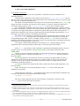
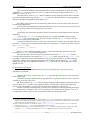
ARIANE User Manual
I am to work with ARIANE…
Here follow some indications which can make easier
its implementation and use!
B. BLANKE and N. GRIMA
Laboratoire de Physique des Océans
Brest, France
Contact: [email protected]
___________________________________________________________________________________________________
1/13
22 September 2005
ARIANE User Manual
1. Spirit of the Lagrangian approach
1. Spirit of the Lagrangian approach
a) Introduction
The ARIANE utility developed at LPO makes it possible to describe from a Lagrangian point of
view the dynamics simulated by an Ocean General Circulation Model (OGCM) as OPA.
Such diagnostics are based on the calculation of multiple trajectories in the modeled velocity
field, with an advection scheme particularly fitted to the three-dimensional nature of the oceanic
circulation [Blanke and Raynaud, 1997] and to an effective description of a water mass from the
particles which form it [Döös, 1995].
Within the framework of the European program TRACMASS1 (June 1998 - May 2001), these
analyses were applied to various classes of OGCM (an isopycnic and three z-coordinate models), over
distinct domains (the Mediterranean Sea and the global ocean), with various spatial resolutions.
One of the key problems of the Lagrangian tracing of ocean water masses is posed by the
characteristic times of large scale advection. The Lagrangian trajectories must be integrated for
sufficiently a long time to describe the full range of the movements at a basin or global scale. This
means several hundreds, even thousands of years, whereas direct OGCM simulations seldom exceed a
few tens of years because of CPU time constraints or drift problems.
One way to by-pass this difficulty is the development of diagnostics run from the archive of the
model fields (and associated tracers), with repeated loops over the archived period (usually a
climatological year). This offline approach is tempting because of its flexibility, but it raises
nevertheless two major questions:
• What is the impact of unresolved frequencies (in the archived output) on the subsequent
offline trajectory calculations and other Lagrangian diagnostics?
• Can one be satisfied with such an approach in the case of an archive limited to a fraction of a
simulation presenting signs of drift (i.e. an imperfect adjustment to the surface forcing) or with strong
interannual variability?
This last point could be addressed by our TRACMASS collaborators and does not concern this
presentation. The contribution of LPO to the methodological section of the same TRACMASS project
allowed us to study the first point in a model with a coarse horizontal resolution (the ORCA2 version
of the OPA model, with a 2° zonal resolution), and without drift (as it was run a in robust-diagnostic
mode) [Valdivieso Da Costa and Blanke, 2003]. We could show that within this framework of
climatological modeling at coarse space resolution, a monthly archive of the velocity field (sampling
appropriately the seasonality the various internal and surface forcing functions) proved to be necessary
for the development of reliable Lagrangian analyses.
b) Advantages of a C grid
The equations of the OPA model are discretized on a C-type grid [Arakawa, 1972]. This mesh
system proves to be ideal for the analytical calculation of successive streamline segments [Blanke and
Raynaud, 1997] from a time sampled velocity field (with period ∆T).
This Lagrangian integration scheme respects the local conservation of mass and thus defines a
judicious tool to carry out water mass tracing. The technique lies on the insemination of a given water
mass (considered on a geographical section) by tens or hundreds of thousands of individual particles
[Döös, 1995; Blanke and Raynaud, 1997], and by assigning to each of them an infinitesimal fraction
of the incoming transport. For a selected set of final destinations (other geographical sections, or the
satisfaction of a hydrological criterion), infinitesimal transports can be combined and allow the
evaluation of directional transports (water flow between two given sections).
c) Individual trajectories
The analytical calculation of streamlines on the model grid, for successive ∆T periods over
which the velocity speed is assumed to remain constant, offers several advantages. This method for
computing trajectories is both fast and accurate: it only calculates positions on the edge of individual
grid cells, and it fully respects the local three-dimensional non-divergence of the flow. The method is
1
“Tracing the water masses of the North Atlantic and the Mediterranean”
___________________________________________________________________________________________________
2/13
22 September 2005
ARIANE User Manual
1. Spirit of the Lagrangian approach
flexible too, and backward integrations can be performed to track the origin of a given current, insofar
as calculations do not involve diffusive phenomena.
By making the assumption of a linear variation of each component of the velocity speed along
each corresponding direction, elementary relations are written to describe the trajectory equations
along the three axes. The integration in time of these equations allows binding each co-ordinate (x, y,
or z) to time inside each model gridcell. Crossing times in each direction are evaluated independently
by imposing as a possible final position each of the six sides of the gridcell. The minimum of these
estimates gives the exact crossing time, and allows the accurate calculation of the final position on the
exit side.
d) Detailed calculations [Blanke and Raynaud, 1997]
Usual ways to compute trajectories from GCM outputs involve first the interpolation of the
three-dimensional velocity at the location of a given particle, then the advection of this particle in the
direction of the current. Such methods require accurate interpolation and advection schemes to
minimize possible cumulative errors in the computation of the trajectories. In the present study, we
take advantage of the C grid used for discretizations in the OPA model to compute analytically
trajectories from model outputs. The algorithm calculates true trajectories for a given stationary
velocity field through the exact computation of three-dimensional streamlines. Under the assumption
of stationarity, such streamlines indeed represent trajectories of particles advected by the given
velocity field. The three components of the velocity are known over the six faces of each cell. The
nondivergence of the velocity field then ensures continuous trajectories within this cell. We develop
here some equations with the tensorial formalism used in the OPA model [Marti et al. 1992], which
allows a more general approach than a simple Cartesian view, with for instance the description of a
distorted grid over the sphere. Using the same notations as Marti et al. [1992], the divergence of the
threedimensional velocity field V = (U, V, W) is expressed as
ΔV = b -1 [∂i(e2 e3 U) + ∂j(e1 e3 V) + ∂k(e1 e2 W)],
(A.1)
where n = i, j, or k refers to the grid index for the three axes; n refers to the corresponding finite
difference; e1, e2, and e3 are the scale factors (in the three directions) computed at each velocity grid
point; and b is the product e1 e2 e3 computed at the center of a given cell (“temperature” grid point).
For any choice of the grid, the non-divergence of the flow now simply writes as
∂iF + ∂jG + ∂kH = 0,
(A.2)
where F, G, and H designate the transports in the three directions, with F = e2 e3 U, etc. We assume
now that the three components of the transport vary linearly between two opposite faces of one
individual cell. This hypothesis respects the local three-dimensional non-divergence of the flow. It
means that, within a given cell, F depends linearly on i, G depends linearly on j, and H depends
linearly on k, where i, j, and k are considered as fractional within the cell (i.e., as non integer). In the
cell extending from i = 0 to i = 1, one can write for instance for F
F(r) = F0 + r ΔF,
(A.3)
with r ∈ [0, 1] and F(0) = F0, and where ΔF stands for F(1) - F(0). One can also write the equation
linking position and velocity, namely dx/dt = U, for the transport
dr/ds = F,
(A.4)
-1
with s = (e1 e2 e3) t and x = e1 r. With some adequate initial conditions, for example, r = 0 for s = 0,
one can combine (A.3) and (A.4) and find the time dependency of r within the considered cell
r = F0 ΔF -1 [exp(ΔF s) – 1].
(A.5a)
If ∆F = 0, only the limit of (A.5a) for ∆F → 0 is to be considered
r = F0 s.
(A.5b)
Similar relationships are of course obtained along both other directions. Since these expressions
only apply in one individual cell, one also has to determine the time when a given particle switches to
another cell, or equivalently the time when r is equal to its exit value (here r = 1). Time dependency is
obtained from a different writing of (A.4):
ds = F -1 dr.
(A.6)
Using (A.3), one obtains the following expression for ds:
ds = (F ΔF) -1 dF.
(A.7)
___________________________________________________________________________________________________
3/13
22 September 2005
ARIANE User Manual
1. Spirit of the Lagrangian approach
A crossing time in the zonal direction can only be obtained if F(1) and F(0) have the same sign,
and this implies F ≠ 0 in the cell. If this condition is not verified for F, the three-dimensional nondivergence of the velocity field ensures that at least one other direction satisfies it. One can assume
that this condition is checked in the zonal direction. The pseudo time s is then related to the transport F
by
s = ΔF -1 ln(F / F0).
(A.8)
The crossing time in this direction corresponds to the moment when the transport reaches the
exit face value, F(1):
Δs = ΔF -1 ln([F0 + ΔF] / F0),
(A.9a)
or, if ∆F = 0, its limit when ∆F → 0:
Δs = 1 / F0.
(A.9b)
As previously mentioned, at least one of the three crossing times is to be defined through such a
formulation. The shortest one defines the traveling time in the considered cell. Thus, if the particle
first attains the zonal extremity of the cell, its positions on the meridional and vertical axes are
deduced from the equations of the trajectories using s = ∆s. Computations are done for the next cell,
with a starting point equal to the exit point of the previous one, and the “age” of the particle is
regularly updated summing the expressions (A.9) obtained for ∆s.
e) Quantitative diagnostics
Quantitative results are obtained by increasing considerably the number of particles (possibly up
to several millions), following the technique developed by Döös [1995] and Blanke and Raynaud
[1997]. Due to water incompressibility, one given particle with an infinitesimal section is to conserve
its infinitesimal mass along its trajectory. As a current can be entirely determined by the particles that
compose it, with well-defined characteristics (position, velocity, and other scalars), the transport of a
given water mass can be calculated from its own particles and their associated infinitesimal transport.
For most of the quantitative diagnostics run with ARIANE, the area of each grid cell, for a given
instant and with a given transport Ti, is described with particles whose Ni3 initial positions are
homogeneously distributed in space and time (with lagged departure times). The number of
subdivisions along each direction, Ni, satisfies
Ti/Ni3 ≤ T0
(A.10)
where T0 is the prescribed maximum transport associated with a single particle. The total number of
particles used to describe the water mass is the sum of the Ni’s, over the relevant grid points of the
section and the total number of instants (as for instance the 12 months of a climatological year),
knowing that a homogeneous space-time distribution of particles is used in each sub gridcell [Blanke
et al., 1999].
The best positioning of the particles over an initial section is indeed the one that gives the
highest accuracy in the computation of the transports associated with the circulation, for a reasonable
number of initial positions. A measurement of the accuracy is the difference between “section to
section” transports computed for a stationary velocity field with both forward and backward
integrations, as both transports are virtually equal. “Constant number of particles by grid cell” and
“spatially homogeneous distributions” are not satisfactory because they may use too few (many)
particles to describe regions of weak (slow) currents. A sophisticated approach would distribute
particles so that they have the same transport, thus grouping them in regions where the velocity is the
highest.
f) Lagrangian mass streamfunctions
We compute trajectories for all the particles and sum algebraically the Ti on each junction of
two model gridcells, on the velocity grid points of the staggered C-grid [Arakawa 1972]. Northward
and eastward movements are counted positive, while southward or westward movements are counted
negative. We obtain a three-dimensional transport field that corresponds to the flow of the water mass
in study, within the domain of integration of the trajectories. As one particle entering one model grid
cell through one of its six faces has to leave it (by another face), the transport field exactly satisfies
∂iTx + ∂jTy + ∂kTz = 0,
(A.11)
where Tx , Ty , and Tz designate the directional flows (in sverdrups) in the three directions, and where i,
j, or k refers to the grid index for the three axes. Integrating this field along a selected direction (either
___________________________________________________________________________________________________
4/13
22 September 2005
ARIANE User Manual
1. Spirit of the Lagrangian approach
the vertical, zonal, or meridional axis), we obtain a two-dimensional non-divergent field that we study
by means of a streamfunction. For a vertically integrated transport or a zonally integrated transport, we
define ψh and ψyz, respectively, with
∂iψh = Σk Ty ; ∂jψh = - Σk Tx
∂iψyz = Σk Tz ; ∂jψyz = - Σk Ty
(A.12)
and contours of ψh or ψyz provide an adequate view of the movement in projection onto the selected
plane. As contours cannot cross each other (by construction of a streamfunction), the more accurately
and selectively we define the initial conditions of the particles, the more similar the contours are to
actual projections of trajectories. The choice of a horizontal projection usually turns out judicious, but
an additional plane of projection or plots of selected individual trajectories may be helpful in plotting
the precise movement of the water mass.
g) LPO publications related to the use of ARIANE
Blanke, B. and S. Raynaud, 1997: Kinematics of the Pacific Equatorial Undercurrent: a Eulerian and
Lagrangian approach from GCM results. Journal of Physical Oceanography, 27, 1038-1053.
Blanke, B., M. Arhan, G. Madec, and S. Roche, 1999: Warm water paths in the equatorial Atlantic as
diagnosed with a general circulation model. Journal of Physical Oceanography, 29, 2753-2768.
Blanke, B., S. Speich, G. Madec, and K. Döös, 2001: A global diagnostic of ocean mass transfers.
Journal of Physical Oceanography, 31, 1623-1642.
Blanke, B., S. Speich, G. Madec, and R. Maugé, 2002: A global diagnostic of interior ocean
ventilation. Geophysical Research Letters, 29, 10.1029/2001GL013727.
Blanke, B., M. Arhan, A. Lazar, and G. Prévost, 2002: A Lagrangian numerical investigation of the
origins and fates of the salinity maximum water in the Atlantic. Journal of Geophysical
Research, 107, 10.1029/2002JC001318.
Blanke, B., M. Arhan, S. Speich, and K. Pailler, 2002: Diagnosing and picturing the North Atlantic
segment of the global conveyor belt by means of an ocean general circulation model. Journal of
Physical Oceanography, 32, 1430-1451.
Blanke, B., S. Speich, A. Bentamy, C. Roy, and B. Sow, 2005: Modeling the structure and variability
of the southern Benguela upwelling using QuikSCAT wind forcing. Journal of Geophysical
Research, 110, doi:10.1029/2004JC002529.
Friocourt, Y., S. Drijfhout, B. Blanke, and S. Speich, 2005: Water mass export from Drake Passage to
the Atlantic, Indian, and Pacific Oceans: A Lagrangian model analysis. Journal of Physical
Oceanography, 35, 1206-1222.
Izumo, T., J. Picaut, and B. Blanke, 2002: Tropical pathways, equatorial undercurrent variability and
the 1998 La Niña. Geophysical Research Letters, 29, 10.1029/2002GL015073.
Radenac, M.-H., Y. Dandonneau, and B. Blanke, 2005: Displacements and transformations of nitraterich and nitrate-poor water masses in the tropical Pacific during the 1997 El Ninño. Ocean
Dynamics, 55, 34-46.
Rodgers, K. B., B. Blanke, G. Madec, O. Aumont, P. Ciais, and J.-C. Dutay, 2003: Extratropical
sources of equatorial Pacific upwelling in an OGCM. Geophysical Research Letters, 30,
10.1029/2002GL016003.
Rodgers, K. B., O. Aumont, G. Madec, C. Menkes, B. Blanke, P. Monfray, J. C. Orr, and D. P.
Schrag, 2004: Radiocarbon as a thermocline proxy for the eastern equatorial Pacific.
Geophysical Research Letters, 31.
Speich, S., B. Blanke, and G. Madec, 2001: Warm and cold water routes of a GCM thermohaline
conveyor belt. Geophysical Research Letters, 28, 311-314.
Speich, S., B. Blanke, P. De Vries, K. Döös, S. Drijfhout, A. Ganachaud, and R. Marsh, 2002: Tasman
leakage: a new route in the global ocean conveyor belt. Geophysical Research Letters, 29,
doi:10.1029/2001GL014586.
Valdivieso Da Costa, M. and B. Blanke, 2004: Lagrangian methods for flow climatologies and
trajectory error assessment. Ocean Modelling, 6, 335-358.
h) Cited references
___________________________________________________________________________________________________
5/13
22 September 2005
ARIANE User Manual
1. Spirit of the Lagrangian approach
Döös, K., 1995: Inter-ocean exchange of water masses. Journal of Geophysical Research, 100,
13499–13514.
Arakawa, A., 1972: Design of the UCLA general circulation model. Numerical simulation of weather
and climate. Tech. Rep. 7, Dept. of Meteorology, University of California, Los Angeles, 116 pp.
___________________________________________________________________________________________________
6/13
22 September 2005
ARIANE User Manual
2. Things I should know before I compile ARIANE
2. Things I should know before I compile ARIANE
I must edit the namelist and adjust each variable to my specific needs. Here are the most
important variables:
• imt, jmt, kmt and lmt: the dimensions of the grid (three space dimensions, one time dimension)
must be correct and consistent with the fields prepared for ARIANE.
• tunit defines a convenient unit of time (in seconds), usually one day (86400.).
• ntfic is the sampling time (in number of tunit) for the available velocity and tracer fields.
Therefore, the product ntfic×tunit must give in seconds the period covered by each velocity and tracer
time sample.
• zsigma gives the reference immersion (in meters) used by ARIANE (in particular in the output
files) for the recalculation (if needed) of density. The unit is σn, where n corresponds to the depths
expressed in thousands of meters.
• nmax, maxsegm and maxsect allow the maximum dimensioning of arrays used by ARIANE in
its Lagrangian calculations. An error message in the course of execution will normally inform me of
their possible bad calibration, and I will then have to increase their value.
Some boolean keys can be used to activate a few additional ARIANE functionalities:
• key_alltracers should be used (“true” value) if I want to activate diagnostics related to tracers.
Otherwise, the Lagrangian tracing will only deal with kinematics.
• key_periodic and key_jfold allow me to inform ARIANE about zonal grid periodicity and
meridional grid folding, respectively (as introduced in the OPA model).
• key_computew asks ARIANE to diagnose the vertical velocity by the vertical integration of the
horizontal divergence, from the ocean floor (where the vertical velocity is expected to be 0) to the
surface. In this case, I may obtain a non zero vertical velocity residual and may need to use a
horizontal “lid” to intercept “evaporating” particles (see the discussion below). If key_computew is
“false”, I understand that ARIANE will use the vertical velocity provided in the input velocity files, and
that this vertical velocity must balance exactly the convergence of the horizontal transport.
• key_ingridt and key_outgridt may be used to modify the convention used by ARIANE for
reading and writing spatial coordinates, respectively. I must understand that ARIANE used by default
its internal system of coordinates related to the velocity gridpoints of a C-grid. I may force the system
of coordinates to be referenced to tracer gridpoints. The latter system may be easier to master for me,
but it is not the standard ARIANE reference.
Indexation system used on the horizontal. Decimal coordinates of the star satisfy
• for a reference on the T grid: i + 1 < it < i + 2 and j < jt < j + 1
• for a reference on the (U, V) grids: i < iu < i + 1 and j - 1 < jv < j
The decimal coordinates then satisfy: it = iu + 0.5 and jt = jv + 0.5
___________________________________________________________________________________________________
7/13
22 September 2005
ARIANE User Manual
2. Things I should know before I compile ARIANE
Indexation system used on the vertical. Decimal coordinates of the star satisfy
• for a reference on the T grid: k < kt < k + 1
• for a reference on the (U, V) grids: k + 1 < kw < k + 2
The decimal coordinates then satisfy: kt = kw - 0.5
• key_sigma should be used if I want ARIANE to calculate its own density field (at reference
level zsigma) from the temperature and salinity read on file. Otherwise, ARIANE will have in central
memory the density field that is read on file.
• key_approximatesigma must be used only if I want ARIANE to use the density array in central
memory for density interpolations. Indeed, ARIANE prefers by default not to interpolate directly
density but to recalculate it from locally interpolated values of temperature and salinity, using its own
density equation and reference level zsigma.
• key_nointerpolstats is used only if I prefer to use of the nearest tracer gridpoint value in tracer
statistics for initial and final positions, instead of a quadri-linear interpolation of several neighboring
gridpoints.
• key_partialsteps is to be used to accommodate partial steps the way they are implemented in
OPA.
• key_unitm3 replaces the standard output unit used for transports (sverdrups) by m3/s.
• key_eco reduces a lot some calculations made by ARIANE and should be used every time I am
not interested in plotting separate streamfunctions for separate final sections. I must understand that it
does not modify the trajectory calculations, but that it has an impact on the information stored on some
of the output files that will be used for subsequent diagnostics.
___________________________________________________________________________________________________
8/13
22 September 2005
ARIANE User Manual
3. After a successful compilation
3. After a successful compilation...
a) Qualitative experiments
Everything seems ready for a first experiment. I will thus try first the calculation of an
individual trajectory.
I add the initial coordinates of my particle to the end of file initial_positions2. Not less
than five values (three spatial indices, one temporal index and a fifth parameter3 that I can choose right
now equal to 1.0) define an initial position.
The format of the spatial indices must respect the convention I may modify with key_ingridt. By
default, the frame of reference uses the three velocity grids (U, V and W). I am aware that lines of
comments (starting with @) in file initial_positions refer to this coordinate system.
For a spatial frame organized on the tracer grid (T), the positioning strategy is intuitive: integer
coordinates correspond to a position at the center of the tracer gridcell bearing the same indices i, j and
k. I will use non integer (float) indices to introduce any shift with respect to this central position4. A
spatial frame organized on the velocity grids matches the internal calculations performed by ARIANE,
but requires use of three references (one along each direction).
The format used to position my initial particle in time is also described in the comments of file
initial_positions. An integer value corresponds to the center of the period covered by the
corresponding sample. Thus, if I have a monthly velocity speed (lmt = 12), a value 4.0 of the time
parameter will initialize the particle at the date of April 15. On the other hand, I would specify the date
of December 31 by using the value 12.5 (or 0.5).
I can require constant-depth calculations for trajectories (i.e., without using the vertical
component of the velocity) by putting a minus sign (-) before the initial vertical index.
In file param, I specify that I want a qualitative experiment (full monitoring of the successive
positions of one or several particles, code QUALITATIVE), for the study of their fate (code
FORWARD).
I do not use for the moment the possibility to restart from the results of a former experiment,
and my initial positions are actually provided by file initial_positions. Therefore I thus use
the code NOBIN.
After having defined a convenient unit of time in seconds (for example 86400, for a day), I
indicate the interval I want between two successive position outputs5 on file for my particles (for
example 10, for 10 days), and the total number of positions I want (for example 20 if I want the
calculation of a 200-day trajectory).
As I want to include in the output file the surface mask of the model (“land” gridpoints), I use
the code MASK.
Lastly, I do not take care of the last parameter of file param since it deals only with
quantitative experiments.
I run the program with script go, providing the name of the experiment (which will denote also
the name of the directory in which the results will be stored):
<prompt> go EXPER01
The result (“land” gridpoints and successive positions for particles) is in the ASCII file
traj.ql, where one line represents one position.
2
I am careful not to let truncated lined at the end of this file. There must be as many lines (not starting with @) as initial
positions. Not more, nor less.
3
This fifth parameter appears only for consistency with the format used in the quantitative experiments run with ARIANE. I
initialize it with an arbitrary value (typically 1.0), while being conscious that it will absolutely not be used in qualitative
calculations.
4
I do not initialize my particles exactly on the corner of a temperature gridcell, insofar as the velocity is imperfectly defined
there. An initial positioning exactly at the center of T gridpoints often proves judicious.
5
As the calculations are analytical, this parameter does not affect the precision of the trajectories calculated by ARIANE. It is
only a parameter used for graphic purposes
___________________________________________________________________________________________________
9/13
22 September 2005
ARIANE User Manual
3. After a successful compilation
Thus, on each line I find the following information: index of the particle (0 stands for “land”
gridpoints), x, y, z, time (in number of cycles6 covered by the velocity field provided to ARIANE, i.e.,
generally, in years), T, S, σn.
I note that I have given to ARIANE initial coordinates on the model grid (mesh indices) but that
the result of the qualitative experiment (traj.ql) is directly expressed in the form of geographical
and time coordinates (longitude, latitude, depth, age).
Everything works perfectly for the time being, and I choose to use the result of this first run to
test backward calculations.
I will start from the final position obtained at the end of the first experiment and I will check if I
succeed to go back to the same initial position as previously.
I use for this new experiment the binary archive (full precision) of the final position of the first
experiment.
I copy the file final.sav in another directory (for example EXPER02) under the name
initial.bin, and I specify now the code BIN 7 instead of NOBIN in param. In this same file, I
use from now on the code BACKWARD.
As I did not modify the FORTRAN code itself, I do not need to compile the code again, and I use
the script go directly (by specifying the name of the new experiment, i.e. the directory where I copied
the initial.bin file:
<prompt> go EXPER02
With a precision within my machine accuracy, I check that I find the same trajectory than
previously in traj.ql, but calculated backward.
The code BIN forces the restarting of all the particles present in initial.bin. If I have
several positions in this file (for example if initial.bin is taken equal to the file final.sav of
a qualitative experiment using several particles), I can go on with a qualitative experiment starting
from only a subset of these positions by using the code SUBBIN instead of BIN in param, and by
listing, line after line, in an additional file named subset, the indices of the particles that I want
indeed to re-use8.
b) Quantitative experiments
Since the qualitative experiments do not pose specific problems, I will run now a first
quantitative experiment...
I activate the code QUANTITATIVE in param, instead of QUALITATIVE, and I go back to
mode FORWARD.
I reactivate the code NOBIN insofar as my quantitative experiment will not use the result of an
experiment previously carried out.
The time parameters in param control only the sampling of the individual trajectories and will
not be used by ARIANE (unlike in the qualitative mode). Consequently, I ignore them and I jump
directly to the last parameter: it defines the precision of the quantitative experiments.
In order to limit the computing time, I use the lowest possible precision by inflating artificially
the maximum value of transport (Tr0, in m3/s) that may be associated with each particle. I use 109 as
recommended. I will be able to refine my results thereafter by reducing this value.
6
I can obtain a trajectory shorter than what I explicitly asked in param if ever my particle is intercepted by ARIANE on the
edges (or at the surface) of the domain covered by the grid. In this case, I will not have any binary archive of the initial
and final positions of this particle (files init.sav and final.sav).
7
Insofar as I use the code BIN, the content of the file initial_positions will be ignored, as ARIANE will use the
position given in intial.bin to start the calculation of the trajectories.
8
In a SUBBIN configuration, I must introduce the indices in subset by order ascending (using for example the UNIX
command sort –n). Otherwise I am likely to see ARIANE blunder badly in the selection of my particles.
___________________________________________________________________________________________________
10/13
22 September 2005
ARIANE User Manual
3. After a successful compilation
The usual purpose of a quantitative experiment is the evaluation of the mass transport
established between an “initial” section of the domain and final interception sections9. For this reason,
I must define for ARIANE a closed sub-volume within my domain of study, whose simplest
formulation is that of a right-angled parallelepiped.
Such sections are defined in the form of segments, forming vertical planes in the Ox (i = it1 to
it2, j= jt0, k = kt1 to kt2) or Oy (i = it0, j = jt1 to jt2, k = kt1 to kt2) directions, or horizontal planes (i = it1
to it2, j = jt1 to jt2, k = kt0).
I will build my sections with such segments, I will assign to each section a sequence number
(with 1 corresponding with the section where the particles will be initialized), I will use a proper
orientation10 for each of them (to inform ARIANE about the localization of the interior and the outside
of the domain of study). I will put this information at the end of file segments.
I can use the utility mkseg to obtain a first fast and reliable definition of segments11.
I run program mkseg0.
I open the output file (segrid) with a suitable text editor, so as to visualize in a convenient
way the integrality of the domain.
I define by hand the sections I want to use, by replacing “ocean” gridpoints by an appropriate
section index. I make sure that the segments related to a same section have a length larger or equal to 2
gridpoints. I am careful to define a closed domain, limited by section indices or by “land” gridpoints.
I end this step by putting a “@” sign on an “ocean” gridpoint located inside the active domain.
This hot spot will allow mkseg to differentiate the interior and the outside of my active domain, and
to give a correct orientation to each segment.
I run mkseg and I sort the output for a better legibility: mkseg | sort
In the event of mistakes while editing segrid, some error messages might be returned, and, in
file segrid, a star “*” should appear in the immediate vicinity of a problem that is found. I must redo
the construction of this file by correcting it the best I can.
With determination, I end up with a clean output (no more error messages), and I copy the result
(namely the coordinates of the segments calculated by mkseg) after12 the lines of comments of file
segments.
I introduce an explicit label for each section (instead of 1section, 2section...), and possibly add a
“lid” as an additional horizontal section of control in order to intercept the particles feeling a vague
desire to evaporate in the atmosphere. For this last section I vary i from 1 to imt, j from 1 to jmt and I
choose kt1 and kt2 equal to kt0 = 0.
Lastly, I check in criter0.h and criter1.h that the activated hydrological criteria are
those I want. For a first test, I may find easier to activate standard values (criter0 = .TRUE. and
criter1 = .FALSE.). I will discover later how to use these criteria more cleverly.
My quantitative experiment is ready to run. I type go EXPER03, after compiling the code if
ever I modified the FORTRAN code.
In result, I find the usual files init.sav and final.sav, containing in a binary format the
initial and final positions of all the particles used in this quantitative experiment.
I look immediately at the contents of the ASCII file stats.qt to find the intensity of the mass
transfers diagnosed from the initial section towards each final section13, as well as elementary statistics
9
The initial section is also used as a section of interception, in order to diagnose any possible recirculation.
A correct orientation of the segments is imperative for the initial section, and optional (but recommended) for the other
(final) sections. The convention for orientation (a positive or negative sign of jt0, it0or kt0) is described in the comments
given in file segments.
11
Unlike ARIANE, the mkseg utility does not handle currently the condition of meridional folding (as activated for instance in
the global version of the OPA model).
12
Like for the file initial_positions, I take care not to introduce truncated lines at the end of this file, and I use as
many lines as the number of segments I want to define.
10
___________________________________________________________________________________________________
11/13
22 September 2005
ARIANE User Manual
3. After a successful compilation
related to the initial and final positions participating in each transfer. I do not pay too much attention
to the very first line of file stats.qt which informs me about a pseudo “total transport”, before
normalization by the time dimensioning parameter lmt.
I find in file init_pos.qt the whole set of initial positions with an ASCII format. Each line
corresponds to one particle, and I recognize, in that order: spatial positioning14 (on the grid, tracer or
velocity, I chose), time positioning (with a convention identical to that defined in
initial_positions), transport allotted by ARIANE, and tracer values interpolated onto the initial
position. The file for final positions final_pos.qt has a similar structure and also shows the
elapsed time (in years), followed by the index of the section of arrival (according to the convention
adopted in file segments).
Files prefixed with xy_*, yz_* ou xz_* include the information necessary to the graphic
representation of the mass transfers achieved towards each section. I will be able to read these files
with a utility like IDL, and to use existing scripts for a fast and easy visualization of the results in the
form of streamlines.
I can now determine tentatively a better value for parameter Tr0. The first experiment (run with
Tr0 = 109 m3/s) gives me a coarse estimate (in sverdrups) of the mass transfers between my initial
section and my final sections. I can thereafter take for Tr0 a value roughly equal to the precision I wish
to obtain on these transfers (for example 10-2 Sv, i.e., 104 m3/s).
I decide to run a new quantitative experiment, and activate new functionalities in ARIANE.
I take the same domain of study, but I choose to use a different section as a starting section.
Insofar as mkseg already did a clean work, I only need to edit file segments, to allocate number 1
(initial section) to the segments defining the new section I want to use for the initialization of the
particles (for example numbered 3 in the former experiment), and to give number 3 to the former
initial section (simple swap of indices).
I also choose to refine the definition of the initial positions by asking ARIANE to keep only the
initial particles corresponding to a temperature warmer than 15.5°C, a density σ4 lower than 45.9 and a
density σ2 larger than 45.84. Therefore, I edit the piece of code criter0.h, and I replace the default
criterion (criter0 = .TRUE.) by the following FORTRAN lines:
t = zinter(tt,hi,hj,hk,hl)
s = zinter(ss,hi,hj,hk,hl)
r4 = sigma(4000.,s,t)
r2 = sigma(2000.,s,t)
criter0 = (t.gt.15.5).AND.(r2.gt.45.840).AND.(r4.le.45.900)
I notice the use of the function zinter, that allows a fine interpolation (trilinear in space and
linear in time) of the tracer fields onto the position of the particle (given by hi, hj, hk and hl), and of
function sigma, that calculates density15 at a given reference level from known salinity and
temperature values.
I also want to intercept during the Lagrangian integration the particles that will see their
temperature warming beyond 16°C. This hydrological interception will be done, if necessary, before
13
I check that the transfers to each final section are expressed in sverdrups, and use the same numerical labeling as the
numbering that I used to define my sections in file segments. A code “0” (meanders) appears next to a code “1”
(1section). I will discover soon, when I use of a hydrological criterion on the initial positions, the reason for this
distinction. I remember for the moment that the destination “0” corresponds geographically to the destination “1”, namely
to my initial section.
14
The coordinates given for the particles are not geographical coordinates, but grid indices expressed on the mesh of my
domain (just like what I used for the initial positioning of my particles in my first qualitative experiment).
15
As I need here to use two distinct immersions to define my density criteria, I cannot work directly with the model array rr,
corresponding to the density field recomputed by ARIANE from the parameter zsigma given in param. I note that the
function sigma enables me to define specific hydrological tests in criter[012].h, while the parameter zsigma will
condition the whole set of density diagnostics provided by ARIANE at the end of the execution (in files stats.qt,
final_pos.qt and init_pos.qt).
___________________________________________________________________________________________________
12/13
22 September 2005
ARIANE User Manual
3. After a successful compilation
reaching any of the geographical sections defined in segments. I edit criter1.h, and replace the
instruction criter1 = .FALSE. with:
t = zinter(tt,hi,hj,hk,hl)
criter1 = (t.gt.16.)
It is also possible to introduce, in one of both criteria (criter0.h or criter1.h), a test on
the geographical position16 of the particle. I will use parameters hi, hj and hk, being careful that they
are defined on the model velocity grid, whatever the convention I could adopt on the format of the
coordinates used for ARIANE input/output files. I will have also to familiarize myself with the fact that
the quantity hk is defined as negative17 in the core of the calculations done by ARIANE, but that fk, the
initial vertical position, is positive.
Having modified the FORTRAN code, I need to recompile it.
Then I run the new experiment: go EXPER04
I look at the results given by file stats.qt. Destinations 0 and 1 present now distinct values
of transport. Destination 0 sums up the transport which recirculates towards the initial section in the
same hydrological range as the one introduced in criter0.h (hence the name “meanders”).
Destination 1 on the contrary accounts, on the same section, for the transport transmitted (“converted”)
into another hydrological class. I see finally that another destination is mentioned. It has the name
Criter1, with an index equal to my total number of control sections plus 1. This is the hydrological
interception carried out by ARIANE on the particles that encountered temperatures larger than 16°C
before reaching any of the final sections.
The statistics (minimal and maximum values) for each field and each destination (for initial and
final positions) enable me to check that my hydrological criteria were indeed respected by ARIANE.
16
17
Although I may test only the parameter of time positioning hl, this process is not at all easy and may even be tricky…
The surface of the ocean thus corresponds to the value hk = –1., while the first tracer levels correspond to hk = –1.5,
hk = –2.5 and hk = –3.5, respectively. This “minus” sign appears only in ARIANE internal calculations (and thus in the
portions of code related to interception criteria), but not in the input/output files.
___________________________________________________________________________________________________
13/13
22 September 2005