Download AMS-LATEX Version 1.2 User's Guide

AMS-LATEX Version 1.2
User’s Guide
American Mathematical Society
January 1995
ii
CONTENTS
Contents
What is ‘AMS-LATEX’, and why would anyone want to use it?
What is ‘AMS-LATEX’ ? . . . . . . . . . . . . . . . . . . . . . . . . . . .
Why would a LATEX user want to bother with AMS-LATEX? . . . . . .
v
v
v
1 How to use AMS-LATEX
1.1 Using an AMS package in a LATEX document . . . . . . . . . . .
1.2 Options for the amsmath package . . . . . . . . . . . . . . . . . .
1
1
1
2 Displayed equations (amsmath package)
2.1 Introduction . . . . . . . . . . . . . . . . . . . . . . . .
2.2 Single equations . . . . . . . . . . . . . . . . . . . . .
2.3 Split equations without alignment . . . . . . . . . . .
2.4 Split equations with alignment . . . . . . . . . . . . .
2.5 Equation groups without alignment . . . . . . . . . . .
2.6 Equation groups with mutual alignment . . . . . . . .
2.7 Alignment building blocks . . . . . . . . . . . . . . . .
2.8 Adjusting tag placement . . . . . . . . . . . . . . . . .
2.9 Vertical spacing and page breaks in multiline displays
2.10 Textual interjections within a display . . . . . . . . . .
2.11 Equation numbering . . . . . . . . . . . . . . . . . . .
.
.
.
.
.
.
.
.
.
.
.
.
.
.
.
.
.
.
.
.
.
.
.
.
.
.
.
.
.
.
.
.
.
.
.
.
.
.
.
.
.
.
.
.
.
.
.
.
.
.
.
.
.
.
.
2
2
3
3
5
5
5
6
7
7
8
8
3 Miscellaneous mathematics features (amsmath package)
3.1 Matrices . . . . . . . . . . . . . . . . . . . . . . . . . . . .
3.2 Math spacing commands . . . . . . . . . . . . . . . . . . .
3.3 Over and under arrows . . . . . . . . . . . . . . . . . . . .
3.4 Dots . . . . . . . . . . . . . . . . . . . . . . . . . . . . . .
3.5 Nonbreaking dashes . . . . . . . . . . . . . . . . . . . . .
3.6 Accents in math . . . . . . . . . . . . . . . . . . . . . . .
3.7 Roots . . . . . . . . . . . . . . . . . . . . . . . . . . . . .
3.8 Boxed formulas . . . . . . . . . . . . . . . . . . . . . . . .
3.9 Extensible arrows . . . . . . . . . . . . . . . . . . . . . . .
3.10 Affixing symbols to other symbols . . . . . . . . . . . . .
3.11 Fractions and related constructions . . . . . . . . . . . . .
3.12 Continued fractions . . . . . . . . . . . . . . . . . . . . . .
3.13 Smash options . . . . . . . . . . . . . . . . . . . . . . . .
3.14 Delimiters . . . . . . . . . . . . . . . . . . . . . . . . . . .
.
.
.
.
.
.
.
.
.
.
.
.
.
.
.
.
.
.
.
.
.
.
.
.
.
.
.
.
.
.
.
.
.
.
.
.
.
.
.
.
.
.
.
.
.
.
.
.
.
.
.
.
.
.
.
.
9
9
10
11
11
11
12
12
13
13
13
13
14
15
15
.
.
.
.
.
.
.
.
.
.
.
4 Operator names (amsopn, amsmath packages)
17
4.1 Defining new operator names . . . . . . . . . . . . . . . . . . . . 17
4.2 \mod and its relatives . . . . . . . . . . . . . . . . . . . . . . . . . 18
iii
CONTENTS
5 The \text command (amstext, amsmath packages)
18
6 The \boldsymbol command (amsbsy, amsmath packages)
18
7 Integrals and sums (amsmath, amsintx packages)
7.1 Multiple integral signs . . . . . . . . . . . . . . .
7.2 Multiline subscripts and superscripts . . . . . . .
7.3 The \sideset command . . . . . . . . . . . . . .
7.4 The amsintx package . . . . . . . . . . . . . . .
.
.
.
.
.
.
.
.
.
.
.
.
.
.
.
.
.
.
.
.
.
.
.
.
.
.
.
.
.
.
.
.
.
.
.
.
8 Commutative diagrams (amscd package)
19
19
19
20
20
20
9 Using math fonts
21
9.1 Introduction . . . . . . . . . . . . . . . . . . . . . . . . . . . . . . 21
9.2 Recommended use of math font commands . . . . . . . . . . . . 21
10 Theorems and related structures (amsthm package)
10.1 Introduction . . . . . . . . . . . . . . . . . . . . . . .
10.2 The \newtheorem command . . . . . . . . . . . . . .
10.3 Numbering modifications . . . . . . . . . . . . . . .
10.4 Changing styles for theorem-like environments . . . .
10.5 Proofs . . . . . . . . . . . . . . . . . . . . . . . . . .
.
.
.
.
.
.
.
.
.
.
.
.
.
.
.
.
.
.
.
.
.
.
.
.
.
.
.
.
.
.
.
.
.
.
.
22
22
23
23
24
25
A Installation instructions
A.1 Introduction . . . . . . . . . . . . . . . . . . . .
A.2 Putting files in a suitable place on your system
A.3 Testing . . . . . . . . . . . . . . . . . . . . . .
A.4 Extra math fonts . . . . . . . . . . . . . . . . .
A.5 Memory requirements . . . . . . . . . . . . . .
A.6 Files included in this distribution . . . . . . . .
.
.
.
.
.
.
.
.
.
.
.
.
.
.
.
.
.
.
.
.
.
.
.
.
.
.
.
.
.
.
.
.
.
.
.
.
.
.
.
.
.
.
27
27
27
27
27
27
28
B Error messages and
B.1 General remarks
B.2 Error messages .
B.3 Wrong output . .
.
.
.
.
.
.
.
.
.
.
.
.
.
.
.
.
.
.
output problems
29
. . . . . . . . . . . . . . . . . . . . . . . . . . . 29
. . . . . . . . . . . . . . . . . . . . . . . . . . . 30
. . . . . . . . . . . . . . . . . . . . . . . . . . . 34
C Other useful items for mathematical documents
35
C.1 AMS documentclasses (amsart, amsbook, amsproc) . . . . . . . . 35
C.2 Extra math fonts (the AMSFonts collection) . . . . . . . . . . . . 36
C.3 Syntax checking (the syntonly package) . . . . . . . . . . . . . . 36
C.4 Verbatim and comments (the verbatim package) . . . . . . . . . 36
C.5 Commutative diagrams and other diagrams (packages diagram,
xypic, pstricks) . . . . . . . . . . . . . . . . . . . . . . . . . . . 36
iv
CONTENTS
D Where to find other information
36
D.1 Technical notes . . . . . . . . . . . . . . . . . . . . . . . . . . . . 37
D.2 Differences between AMS-LATEX version 1.1 and AMS-LATEX version 1.2 . . . . . . . . . . . . . . . . . . . . . . . . . . . . . . . . 37
E Getting help
37
E.1 Further information . . . . . . . . . . . . . . . . . . . . . . . . . 37
Bibliography
38
Index
39
WHAT IS ‘AMS-LATEX’ ?
v
What is ‘AMS-LATEX’, and why would anyone want to use
it?
What is ‘AMS-LATEX’ ?
The name AMS-LATEX is used for convenience to describe a set of loosely
related files that are distributed together by the American Mathematical Society.
Basically they may be described as miscellaneous enhancements to LATEX for
superior information structure of mathematical documents and superior printed
output. Because AMS-LATEX is an extension for LATEX, which in turn is a ‘macro
package’ for the TEX typesetting program, it follows that in order to use any of
the pieces of AMS-LATEX you need to have TEX and LATEX installed first.
LATEX by itself does a rather good job of typesetting mathematics, compared
to non-TEX-based software; it doesn’t add much, however, to the basic set of
mathematical capabilities that it adopted from the Plain TEX macro package.
At the same time that LATEX was being developed by Leslie Lamport (roughly
1982–1986), the American Mathematical Society was throwing its resources into
the development of a different macro package known as AMS-TEX, written by
Michael Spivak. By 1987 or so it became evident that AMS-TEX and LATEX had
complementary feature sets: AMS-TEX focused on the typesetting of math formulas and on fine-tuning typically done by publishers, and was relatively weak
in other areas (for example no automatic numbering or cross-reference facilities); LATEX focused on document structure and logical markup of text, and had
a comparatively limited set of features for dealing with math formula contents.
This situation led to dissatisfaction among both AMS-TEX and LATEX users who
saw desirable features tantalizingly out of reach in the other macro package. So
the American Mathematical Society looked into the question of producing some
sort of combination of the two macro packages that would better serve mathematicians in their writing tasks. The decision that was eventually taken was to
graft the mathematical capabilities of AMS-TEX onto the base stock of LATEX
through an extension package: AMS-LATEX. Most of the programming work
was done by Frank Mittelbach and Rainer Sch¨
opf in 1989–1990 and version 1.0
of AMS-LATEX was released in mid-1990.
Why would a LATEX user want to bother with AMS-LATEX?
If you are just starting out as a LATEX user, you’ll probably have to take our
word for this (or the word of friends and colleagues), but:
If your writing contains a significant proportion of mathematics, and you
care about the quality of the printed results, then sooner or later you’ll find
shortcomings in standard LATEX and want to remedy them. Chances are that
at least the first few of the shortcomings you encounter will be ones that are
already addressed by an AMS-LATEX package. If you want to have maximum
mathematical typesetting power ready at hand, rather than stop to cast about
vi
WHAT IS ‘AMS-LATEX’ ?
for a solution whenever you run into some unusual demand in your writing, then
AMS-LATEX will go a long way toward meeting your needs.
If you are a long-time LATEX user and have lots of mathematics in what you
write, then you may recognize solutions for some familiar problems in this list
of AMS-LATEX features:
• A convenient way to define new ‘operator name’ commands analogous to
\sin and \lim, including proper side spacing and automatic selection of
the correct font style and size (even when used in sub- or superscripts).
• Multiple substitutes for the eqnarray environment to make various kinds
of equation arrangements easier to write.
• Equation numbers automatically adjust up or down to avoid overprinting
on the equation contents (unlike eqnarray).
• Spacing around equals signs matches the normal spacing in the equation
environment (unlike eqnarray).
• A way to produce multiline subscripts as are often used with summation
or product symbols.
• An easy way to substitute a variant equation number for a given equation
instead of the automatically supplied number.
• An easy way to produce subordinate equation numbers of the form (1.3a)
(1.3b) (1.3c) for selected groups of equations.
• A \boldsymbol command for printing bold versions of individual symbols,
including things like ∞ and lowercase Greek letters.
• An amsthm package that provides a useful proof environment and some
enhancements to the \newtheorem command: support for multiple theorem styles in a single document and for unnumbered theorem types.
1. HOW TO USE AMS-LATEX
1
—1—
How to use AMS-LATEX
1.1
Using an AMS package in a LATEX document
A ‘package’ in LATEX terminology is an extension written in such a form that
it can be used via the \usepackage command. Many of the principal features of AMS-LATEX are provided in separate packages so that they can be used
individually on demand. The amsmath package is perhaps the single most noteworthy package, as it subsumes the amstext, amsbsy, and amsopn packages, and
provides a number of other enhancements for mathematical typesetting. The
current list of packages is:
amsmath Defines extra environments for multiline displayed equations, as well
as a number of other enhancements for math.
amstext Provides a \text command for typesetting a fragment of text inside
a display.
amsbsy Defines \boldsymbol and \pmb ‘poor man’s bold’ commands.
amsopn Provides \DeclareMathOperator for defining new ‘operator names’
like \sin and \lim.
amsthm Provides a proof environment and extensions for the \newtheorem
command.
amsintx Provides more descriptive command syntax for integrals and sums.
amscd Provides a CD environment for simple commutative diagrams (no
support for diagonal arrows).
amsxtra Provides certain odds and ends such as \fracwithdelims and
\accentedsymbol.
upref Makes \ref print cross-reference numbers always in an upright/roman
font regardless of context.
1.2
Options for the amsmath package
The amsmath package has the following options:
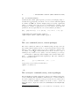
centertags (default) For a split equation, place equation numbers vertically
centered on the total height of the equation.
tbtags ‘Top-or-bottom tags’: For a split equation, place equation numbers level
with the last (resp. first) line, if numbers are on the right (resp. left).
sumlimits (default) Place the subscripts and superscripts of summation symbols above and below, in displayed
equations.
Q `
N L This option also affects
other symbols of the same type— , , , , and so forth—but excluding integrals (see below).
2
2. DISPLAYED EQUATIONS (AMSMATH PACKAGE)
nosumlimits Always place the subscripts and superscripts of summation-type
symbols to the side, even in displayed equations.
intlimits Like sumlimits, but for integral symbols.
nointlimits (default) Opposite of intlimits.
namelimits (default) Like sumlimits, but for certain ‘operator names’ such as
det, inf, lim, max, min, that traditionally have subscripts placed underneath when they occur in a displayed equation.
nonamelimits Opposite of namelimits.
To use one of these package options, put the option name in the optional argument of the \usepackage command—e.g., \usepackage[intlimits]{amsmath}.
The amsmath package also recognizes the following options which are normally selected (implicitly or explicitly) through the \documentclass command,
and thus need not be repeated in the option list of the \usepackage{amsmath}
statement.
leqno Place equation numbers on the left.
reqno Place equation numbers on the right.
fleqn Position equations at a fixed indent from the left margin rather than
centered in the text column.
For symmetry there should perhaps be a centereqn option as well, to balance with fleqn, but as things currently stand there doesn’t seem to be a
genuine need for it.
—2—
Displayed equations (amsmath package)
2.1
Introduction
The amsmath package provides a number of additional displayed equation structures beyond the basic equation and eqnarray environments provided in basic
LATEX. The augmented set includes:
equation
gather
multline
split
align
flalign
alignat
(Although the standard eqnarray environment remains available, align or
split are recommended instead.)
Except for split, each environment has both starred and unstarred forms,
where the unstarred forms have automatic numbering using LATEX’s equation
3
2. DISPLAYED EQUATIONS (AMSMATH PACKAGE)
counter. You can suppress the number on any particular line by putting \notag
before the \\; you can also override it with a tag of your own using \tag{hlabel i},
where hlabel i means arbitrary text such as $*$ or ii used to “number” the
equation. There is also a \tag* command that causes the text you supply to
be typeset literally, without adding parentheses around it. \tag and \tag*
can also be used within the unnumbered versions of all the amsmath alignment
structures. Some examples of the use of \tag may be found in the AMS-LATEX
sample files testmath.tex and subeqn.tex.
2.2
Single equations
The equation environment is for a single equation with an automatically generated number. The equation* environment is the same except for omitting
the number.1
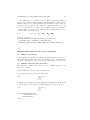
2.3
Split equations without alignment
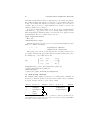
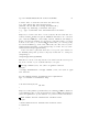
The multline environment is a variation of the equation environment used for
equations that don’t fit on a single line. The first line of a multline will be at
the left margin and the last line at the right margin, except for an indention on
both sides in the amount of \multlinegap. Intermediate lines will be centered
independently within the display width. However, it’s possible to force a line to
the left or right with commands \shoveleft, \shoveright. These commands
take the entire line as an argument, up to but not including the final \\; for
example
(2.10)
A
B
C
D
\begin{multline}
\framebox[.65\columnwidth]{A}\\
\framebox[.5\columnwidth]{B}\\
\shoveright{\framebox[.55\columnwidth]{C}}\\
\framebox[.65\columnwidth]{D}
\end{multline}
The value of \multlinegap can be changed using LATEX’s \setlength and
\addtolength commands. If the multline contains more than two lines, any
lines other than the first and last will be centered individually between the
margins (except when the fleqn option is in effect).
1 Basic L
AT X doesn’t provide an equation* environment, but rather a functionally equivE
alent environment named displaymath.
4
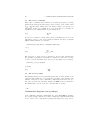
2. DISPLAYED EQUATIONS (AMSMATH PACKAGE)
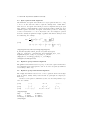
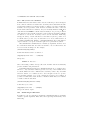
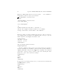
Table 2.1. Comparison of displayed equation environments (vertical lines indicating nominal margins)
\begin{equation*}
a=b
\end{equation*}
\begin{equation}
a=b
\end{equation}
\begin{equation}\label{xx}
\begin{split}
a& =b+c-d\\
& \quad +e-f\\
& =g+h\\
& =i
\end{split}
\end{equation}
\begin{multline}
a+b+c+d+e+f\\
+i+j+k+l+m+n
\end{multline}
\begin{gather}
a_1=b_1+c_1\\
a_2=b_2+c_2-d_2+e_2
\end{gather}
\begin{align}
a_1& =b_1+c_1\\
a_2& =b_2+c_2-d_2+e_2
\end{align}
\begin{align}
a_{11}& =b_{11}&
a_{12}& =b_{12}\\
a_{21}& =b_{21}&
a_{22}& =b_{22}+c_{22}
\end{align}
\begin{flalign*}
a_{11}& =b_{11}&
a_{12}& =b_{12}\\
a_{21}& =b_{21}&
a_{22}& =b_{22}+c_{22}
\end{flalign*}
a=b
(1)
a=b
a=b+c−d
+e−f
=g+h
(2)
=i
(3) a + b + c + d + e + f
+i+j +k+l+m+n
(4)
(5)
a 1 = b 1 + c1
a2 = b2 + c2 − d2 + e2
(6)
(7)
a1 = b 1 + c1
a2 = b2 + c2 − d2 + e2
(8)
a11 = b11
a12 = b12
(9)
a21 = b21
a22 = b22 + c22
a11 = b11
a21 = b21
a12 = b12
a22 = b22 + c22
5
2. DISPLAYED EQUATIONS (AMSMATH PACKAGE)
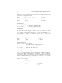
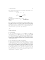
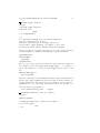
2.4
Split equations with alignment
Like multline, the split environment is for single equations that are too long
to fit on one line and hence must be split into multiple lines. Unlike multline, however, the split environment provides for alignment among the split
lines, using & to mark alignment points, as usual. In addition, unlike the other
amsmath equation structures, the split environment provides no numbering,
because it is intended to be used only inside some other displayed equation
structure, usually an equation, align, or gather environment, which provides
the numbering. For example:
1 X
(−1)l (n − l)p−2
2n
(2.11)
l=0
p Y
ni
X
n
Hc =
l1 +···+lp =l i=1
li
p
i
h
X
· [(n − l) − (ni − li )]ni −li · (n − l)2 −
(ni − li )2 .
j=1
\begin{equation}\label{e:barwq}\begin{split}
H_c&=\frac{1}{2n} \sum^n_{l=0}(-1)^{l}(n-{l})^{p-2}
\sum_{l _1+\dots+ l _p=l}\prod^p_{i=1} \binom{n_i}{l _i}\\
&\quad\cdot[(n-l )-(n_i-l _i)]^{n_i-l _i}\cdot
\Bigl[(n-l )^2-\sum^p_{j=1}(n_i-l _i)^2\Bigr].
\end{split}\end{equation}
2.5
Equation groups without alignment
The gather environment is used for a group of consecutive equations when there
is no alignment desired among them; each one is centered separately within the
text width (see Table 2.1).
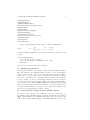
2.6
Equation groups with mutual alignment
The align environment is used for two or more equations when vertical alignment is desired; usually binary relations such as equal signs are aligned (see
Table 2.1).
To have several equation columns side-by-side, use extra ampersands to separate the columns:
(2.12)
(2.13)
(2.14)
x=y
0
X=Y
0
x =y
x + x0 = y + y 0
0
a=b+c
0
X =Y
X + X0 = Y + Y 0
\begin{align}
x&=y
& X&=Y
& a&=b+c\\
x’&=y’
& X’&=Y’
& a’&=b\\
x+x’&=y+y’ & X+X’&=Y+Y’ & a’b&=c’b
\end{align}
a0 = b
a0 b = c0 b
6
2. DISPLAYED EQUATIONS (AMSMATH PACKAGE)
Line-by-line annotations on an equation can be done by judicious application of
\text inside an align environment:
x = y1 − y2 + y3 − y5 + y8 − . . .
= y0 ◦ y∗
(2.15)
(2.16)
by (2.21)
by (3.1)
= y(0)y 0
(2.17)
by Axiom 1.
\begin{align}
x& = y_1-y_2+y_3-y_5+y_8-\dots
&& \text{by \eqref{eq:C}}\\
& = y’\circ y^*
&& \text{by \eqref{eq:D}}\\
& = y(0) y’
&& \text {by Axiom 1.}
\end{align}
A variant environment alignat allows the space between equation columns
to be explicitly specified. Here the number of equation columns must also be
specified (where the number of ‘columns’ is calculated as (1 + &max )/2 with
&max = maximum number of & markers on any line).
x = y1 − y2 + y3 − y5 + y8 − . . . by (2.21)
= y0 ◦ y∗
by (3.1)
(2.18)
(2.19)
= y(0)y 0
(2.20)
by Axiom 1.
\begin{alignat}{2}
x& = y_1-y_2+y_3-y_5+y_8-\dots
&\quad& \text{by \eqref{eq:C}}\\
& = y’\circ y^* && \text{by \eqref{eq:D}}\\
& = y(0) y’
&& \text {by Axiom 1.}
\end{alignat}
2.7
Alignment building blocks
Some other equation alignment environments, such as aligned and gathered,
construct self-contained units that can be used inside of other expressions, or
set side-by-side. These environments take an optional argument to specify their
vertical positioning with respect to the material on either side. The default is
‘middle’ placement with the vertical midpoint of the total unit falling on the
math axis2 . For example:
α = αα
β = βββββ
versus
γ=γ
2 The
height of the cross-bar in the + symbol.
δ = δδ
η = ηηηηηη
ϕ=ϕ
2. DISPLAYED EQUATIONS (AMSMATH PACKAGE)
7
\begin{equation*}
\begin{aligned}
\alpha&=\alpha\alpha\\
\beta&=\beta\beta\beta\beta\beta\\
\gamma&=\gamma
\end{aligned}
\qquad\text{versus}\qquad
\begin{aligned}[t]
\delta&=\delta\delta\\
\eta&=\eta\eta\eta\eta\eta\eta\\
\varphi&=\varphi
\end{aligned}
\end{equation*}
“Cases” constructions like the following are common in mathematics:
(
0
if r − j is odd,
Pr−j =
(2.21)
r! (−1)(r−j)/2 if r − j is even.
and in the amsmath package there is a cases environment to make them easy
to write:
P_{r-j}=\begin{cases}
0& \text{if $r-j$ is odd},\\
r!\,(-1)^{(r-j)/2}& \text{if $r-j$ is even}.
\end{cases}
Notice the use of \text and the embedded math.
2.8
Adjusting tag placement
Placing equation numbers can be a rather complex problem in multiline displays.
The environments of the amsmath package try hard to avoid overprinting an
equation number on the equation contents, if necessary moving the number
down or up to a separate line. Even so, difficulties in accurately calculating
the profile of an equation can occasionally result in a number placement that
doesn’t look right. So there is a \raisetag command provided to adjust the
vertical position of the current equation number. To move a particular number
up by six points, write \raisetag{6pt}. (This kind of adjustment is fine tuning
like line breaks and page breaks, and should therefore be left undone until your
document is nearly finalized, or you may end up redoing the fine tuning several
times to keep up with changing document contents.)
2.9
Vertical spacing and page breaks in multiline displays
You can use the \\[hdimensioni] command to get extra vertical space between lines in all the amsmath displayed equation environments, as is usual in
LATEX. Unlike eqnarray, the amsmath environments don’t allow page breaks
between lines, unless \displaybreak or allowdisplaybreaks is used. The
8
2. DISPLAYED EQUATIONS (AMSMATH PACKAGE)
philosophy is that page breaks in such situations should receive individual attention from the author. \displaybreak is best placed immediately before
the \\ where it is to take effect. Like LATEX’s \pagebreak, \displaybreak
takes an optional argument between 0 and 4 denoting the desirability of the
pagebreak. \displaybreak[0] means “it is permissible to break here” without
encouraging a break; \displaybreak with no optional argument is the same as
\displaybreak[4] and forces a break.
If you prefer a strategy of letting page breaks fall where they may, even in
the middle of a multi-line equation, then you might put \allowdisplaybreaks
in the preamble of your document. An optional argument 1–4 can be used for
finer control: [1] means allow page breaks, but avoid them as much as possible; values of 2,3,4 mean increasing permissiveness. When display breaks are
enabled with \allowdisplaybreaks, the \\* command can be used to prohibit
a pagebreak after a given line, as usual.
2.10
Textual interjections within a display
The command \intertext is used for a short interjection of one or two lines
of text in the middle of a display alignment. Its salient feature is preservation
of the alignment, which would not happen if you simply ended the display and
then started it up again afterwards. \intertext may only appear right after a
\\ or \\* command. Notice the position of the word “and” in this example.
(2.22)
(2.23)
A1 = N0 (λ; Ω0 ) − φ(λ; Ω0 ),
A2 = φ(λ; Ω0 ) − φ(λ; Ω),
and
(2.24)
A3 = N (λ; ω).
\begin{align}
A_1&=N_0(\lambda;\Omega’)-\phi(\lambda;\Omega’),\\
A_2&=\phi(\lambda;\Omega’)-\phi(\lambda;\Omega),\\
\intertext{and}
A_3&=\mathcal{N}(\lambda;\omega).
\end{align}
2.11
Equation numbering
2.11.1 Numbering hierarchy
In LATEX if you wanted to have equations numbered within sections—that is,
have equation numbers (1.1), (1.2), . . . , (2.1), (2.2), . . . , in sections 1, 2, and
so forth—you could redefine \theequation as suggested in the LATEX manual
[5, §6.3, §C.8.4]:
\renewcommand{\theequation}{\thesection.\arabic{equation}}
This works pretty well, except that the equation counter won’t be reset to
zero at the beginning of a new section or chapter, unless you do it yourself using
3. MISCELLANEOUS MATHEMATICS FEATURES
9
\setcounter. To make this a little more convenient, the amsmath package provides a command \numberwithin. To have equation numbering tied to section
numbering, with automatic reset of the equation counter, the command would
be
\numberwithin{equation}{section}
2.11.2 Cross references to equation numbers
To make cross-references to equations easier, an \eqref command is provided.
This automatically supplies the parentheses around the equation number, and
adds an italic correction if necessary. To refer to an equation that was labeled
with the label e:baset, the usage would be \eqref{e:baset}.
2.11.3 Subordinate numbering sequences
The amsmath package provides also a subequations environment to make it
easy to number equations in a particular group with a subordinate numbering
scheme. For example
\begin{subequations}
...
\end{subequations}
causes all numbered equations within that part of the document to be numbered
(4.9a) (4.9b) (4.9c) . . . , if the preceding numbered equation was (4.8). A \label
command immediately after \begin{subequations} will produce a \ref of the
parent number 4.9, not 4.9a. The counters used by the subequations environment are parentequation and equation and \addtocounter, \setcounter,
\value, etc., can be applied as usual to those counter names. To get anything
other than lowercase letters for the subordinate numbers, use standard LATEX
methods for changing numbering style [5, §6.3, §C.8.4]. For example, redefining
\theequation as follows will produce roman numerals.
\begin{subequations}
\renewcommand{\theequation}{\theparentequation \roman{equation}}
...
—3—
Miscellaneous mathematics features (amsmath package)
3.1
Matrices
The amsmath package provides some environments for matrices beyond the basic
array environment of LATEX. The pmatrix, bmatrix, vmatrix and Vmatrix
have (respectively) ( ), [ ], | |, and k k delimiters built in. For naming consistency
there is a matrix environment sans delimiters. This is not entirely redundant
with the array environment; the matrix environments all use more economical
10
3. MISCELLANEOUS MATHEMATICS FEATURES
horizontal spacing than the rather prodigal spacing of the array environment.
Also, unlike the array environment, you don’t have to give column specifications
for any of the matrix environments; by default you can have up to 10 centered
columns.1 (If you need left or right alignment in a column or other special
formats you must resort to array.)
To produce a small matrix suitable for use in text, there is a smallmatrix
environment (e.g., ac db ) that comes closer to fitting within a single text line
than a normal matrix. Delimiters must be provided; there are no p,b,v,V versions
of smallmatrix. The above example was produced by
\bigl( \begin{smallmatrix}
a&b\\ c&d
\end{smallmatrix} \bigr)
\hdotsfor{hnumber i} produces a row of dots in a matrix spanning the given
number of columns. For example,
a
e
b c d
.......
\begin{matrix} a&b&c&d\\
e&\hdotsfor{3} \end{matrix}
The spacing of the dots can be varied through use of a square-bracket option,
for example, \hdotsfor[1.5]{3}. The number in square brackets will be used
as a multiplier (i.e., the normal value is 1.0).


D1 t
−a12 t2 . . . −a1n tn
 −a21 t1
D2 t
. . . −a2n tn 


(3.1)
 . . . . . . . . . . . . . . . . . . . . . . ,
−an1 t1 −an2 t2 . . .
Dn t
\begin{pmatrix} D_1t&-a_{12}t_2&\dots&-a_{1n}t_n\\
-a_{21}t_1&D_2t&\dots&-a_{2n}t_n\\
\hdotsfor[2]{4}\\
-a_{n1}t_1&-a_{n2}t_2&\dots&D_nt\end{pmatrix}
3.2
Math spacing commands
The amsmath package slightly extends the set of math spacing commands, as
shown below. Both the spelled-out and abbreviated forms of these commands
are robust, and they can also be used outside of math
Abbrev.
\,
\:
\;
Spelled out
\thinspace
\medspace
\thickspace
\quad
\qquad
Example
Abbrev.
\!
Spelled out
\negthinspace
\negmedspace
\negthickspace
Example
1 More precisely: The maximum number of columns in a matrix is determined by the
counter MaxMatrixCols (normal value = 10), which you can change if necessary using LATEX’s
\setcounter or \addtocounter commands.
3. MISCELLANEOUS MATHEMATICS FEATURES
11
For the greatest possible control over math spacing, use \mspace and ‘math
units’. One math unit, or mu, is equal to 1/18 em. Thus to get a negative \quad
you could write \mspace{-18.0mu}.
3.3
Over and under arrows
Basic LATEX provides \overrightarrow and \overleftarrow commands. Some
additional over and under arrow commands are provided by the amsmath package
to fill out the set:
\overleftarrow
\overrightarrow
\overleftrightarrow
3.4
\underleftarrow
\underrightarrow
\underleftrightarrow
Dots
When the amsmath package is used, ellipsis dots should normally be typed as
\dots. Placement (on the baseline or centered) is determined by whatever
follows the \dots. If the next thing is a plus sign or other binary symbol,
the dots will be centered; if it’s any other kind of symbol, they will be on the
baseline.
If the dots fall at the end of a math formula, the next thing is something like
\end or \) or $, which does not give any information about how to place the
dots. Then you must help by using \dotsc for “dots with commas,” or \dotsb
for “dots with binary operators/relations,” or \dotsm for “multiplication dots,”
or \dotsi for “dots with integrals.” For example, the input
Then we have the series $A_1,A_2,\dotsc$,
the regional sum $A_1+A_2+\dotsb$,
the orthogonal product $A_1A_2\dotsm$,
and the infinite integral
\[\int_{A_1}\int_{A_2}\dotsi\].
will produce low dots in the first instance and centered dots in the others, with
the spacing on either side of the dots nicely adjusted:
Then we have the series A1 , A2 , . . . , the regional sum A1 + A2 +
· · · , the orthogonal product A1 A2 · · · , and the infinite integral
Z Z
···.
A1
A2
Specifying dots this way, in terms of their meaning rather than in terms of
their visual placement, is in keeping with the general philosophy of LATEX and
makes documents more easily adaptable to different conventions.
3.5
Nonbreaking dashes
A command \nobreakdash is provided to suppress the possibility of a linebreak
after the following hyphen or dash. For example, if you write ‘pages 1–9’ as
12
3. MISCELLANEOUS MATHEMATICS FEATURES
pages 1\nobreakdash--9 then a linebreak will never occur between the dash
and the 9. You can also use \nobreakdash to prevent undesirable hyphenations in combinations like $p$-adic. For frequent use, it’s advisable to make
abbreviations, e.g.,
\newcommand{\p}{$p$\nobreakdash}% for "\p-adic"
\newcommand{\Ndash}{\nobreakdash--}% for "pages 1\Ndash 9"
%
For "\n-dimensional":
\newcommand{\n}[1]{$n$\nobreakdash-\hspace{0pt}}
The last example shows how to prohibit a linebreak after the hyphen but allow
normal hyphenation in the following word. (It suffices to add a zero-width space
after the hyphen.)
3.6
Accents in math
The following accent commands automatically give good positioning of double
accents:
\Hat
\Breve
\Check
\Bar
\Tilde
\Vec
\Acute
\Grave
\Dot
\Ddot
With the usual non-capitalized math accent commands, the second accent will
ˆ
sometimes be askew; for example: Aˆ (\hat{\hat{A}}). With the amsmath package, if you type \Hat{\Hat{A}} (using the capitalized form for both accents)
ˆˆ
the second accent will be better positioned: A.
This double accent operation is complicated and tends to slow down the
processing of a document. If your document contains many double accents, you
may wish to use the amsxtra package, which provides an \accentedsymbol
command. \accentedsymbol is a sort of hybrid of \newcommand and \savebox;
you use it in the preamble of your document to store the result of the double
accent command in a ‘box’ for quick retrieval.
\accentedsymbol{\Ahathat}{\Hat{\Hat A}}
The commands \dddot and \ddddot are available to produce triple and
quadruple dot accents in addition to the \dot and \ddot accents already available in LATEX.
3.7
Roots
√
In ordinary LATEX the placement of root indices is sometimes not so good: β k
(\sqrt[\beta]{k}). In the amsmath package \leftroot and \uproot allow
you to adjust the position of the root:
\sqrt[\leftroot{-2}\uproot{2}\beta]{k}
√
β
will move the beta up and to the right: k. The negative argument used with
\leftroot moves the β to the right. The units are a small amount that is a
useful size for such adjustments.
13
3. MISCELLANEOUS MATHEMATICS FEATURES
3.8
Boxed formulas
The command \boxed puts a box around its argument, like \fbox except that
the contents are in math mode:
η ≤ C(δ(η) + ΛM (0, δ))
(3.2)
\boxed{\eta \leq C(\delta(\eta) +\Lambda_M(0,\delta))}
3.9
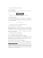
Extensible arrows
\xleftarrow and \xrightarrow produce arrows that extend automatically to
accommodate unusually wide subscripts or superscripts. These commands take
one optional argument (the subscript) and one mandatory argument (the superscript, possibly empty):
(3.3)
n+µ−1
n±i−1
A ←−−−−− B −−−−→ C
T
\xleftarrow{n+\mu-1}\quad \xrightarrow[T]{n\pm i-1}
3.10
Affixing symbols to other symbols
LATEX provides \stackrel for placing a superscript above a binary relation. In
the amsmath package there are somewhat more general commands, \overset
and \underset, that can be used to place one symbol above or below another
symbol, whether it’s a relation or something else. The input \overset{*}{X}
∗
will place a superscript-size ∗ above the X: X; \underset is the analog for
adding a symbol underneath.
See also the description of \sideset in §7.3.
3.11
Fractions and related constructions
3.11.1
Disallowing primitive TEX fraction commands
The six generalized fraction commands \over, \overwithdelims, \atop, \atopwithdelims, \above, \abovewithdelims are expressly forbidden by the amsmath package, as their syntax is decidedly out of place in LATEX; use of the forms
\frac, \binom, \genfrac, and variants is required.2
3.11.2
The \frac, \dfrac, and \tfrac commands
The \frac command, which is in the basic command set of LATEX, takes two
arguments—numerator and denominator—and typesets them in normal fraction
2 Not only is the unusual syntax of the primitive T X fraction commands rather out of
E
place in LATEX, but furthermore that syntax seems to be solely responsible for one of the most
significant flaws in TEX’s mathematical typesetting capabilities: the fact that the current
mathstyle at any given point in a math formula cannot be determined until the end of the
formula, because of the possibility that a following generalized fraction command will change
the mathstyle of the preceding material. As the side effects are a bit technical in nature, they
are discussed in technote.tex rather than here.
14
3. MISCELLANEOUS MATHEMATICS FEATURES
form. The amsmath package provides also \dfrac and \tfrac as convenient
abbreviations for {\displaystyle\frac ... } and {\textstyle\frac ... }.
r
r
1
1
1
1
log2 c(f ) k log2 c(f )
log2 c(f )
log2 c(f )
(3.4)
k
k
k
\begin{equation}
\frac{1}{k}\log_2 c(f)\;\tfrac{1}{k}\log_2 c(f)\;
\sqrt{\frac{1}{k}\log_2 c(f)}\;\sqrt{\dfrac{1}{k}\log_2 c(f)}
\end{equation}
3.11.3 The \binom, \dbinom, and \tbinom commands
For binomial expressions such as nk amsmath has \binom, \dbinom and \tbinom:
k k−1
k k−2
k
2 −
(3.5)
2
+
2
1
2
2^k-\binom{k}{1}2^{k-1}+\binom{k}{2}2^{k-2}
3.11.4 The \genfrac command
The capabilities of \frac, \binom, and their variants are subsumed by a generalized fraction command \genfrac with six arguments. The last two correspond
to \frac’s numerator and denominator; the first two are optional delimiters
(as seen in \binom); the third is a line thickness override (\binom uses this to
set the fraction line thickness to 0—i.e., invisible); and the fourth argument
is a mathstyle override: integer values 0–3 select respectively \displaystyle,
\textstyle, \scriptstyle, and \scriptscriptstyle. If the third argument
is left empty, the line thickness defaults to ‘normal’.
\genfrac{left-delim}{right-delim}{thickness}{mathstyle}
{numerator}{denominator}
To illustrate, here is how \frac, \tfrac, and \binom might be defined.
\newcommand{\frac}[2]{\genfrac{}{}{}{}{#1}{#2}}
\newcommand{\tfrac}[2]{\genfrac{}{}{}{1}{#1}{#2}}
\newcommand{\binom}[2]{\genfrac{(}{)}{0pt}{}{#1}{#2}}
If you find yourself repeatedly using \genfrac throughout a document for a
particular notation, you will do yourself a favor (and your publisher) if you
define a meaningfully-named abbreviation for that notation, along the lines of
\frac and \binom.
3.12
Continued fractions
The continued fraction
(3.6)
1
√
2+
1
√
1
2+ √
2 + ···
15
3. MISCELLANEOUS MATHEMATICS FEATURES
can be obtained by typing
\cfrac{1}{\sqrt{2}+
\cfrac{1}{\sqrt{2}+
\cfrac{1}{\sqrt{2}+\dotsb
}}}
This produces better-looking results than straightforward use of \frac. Left
or right placement of any of the numerators is accomplished by using \cfrac[l]
or \cfrac[r] instead of \cfrac.
3.13
Smash options
The command \smash is used to typeset a subformula and give it an effective
height and depth of zero, which is sometimes useful in adjusting the subformula’s
position with respect to adjacent symbols. With the amsmath package \smash
has optional arguments t and b, because occasionally it is advantageous to be
able to “smash” only the top or only the bottom of something while retaining
the natural depth or height. For example, when adjacent radical symbols are
unevenly sized or positioned because of differences in the height and depth of
their contents,
to make them more consistent. Compare
√
√ \smash
√ can
√be employed
√
√
x + y + z and x + y + z, where the latter was produced by $\sqrt{x}
+ \sqrt{\smash[b]{y}} + \sqrt{z}$.
3.14
Delimiters
3.14.1
Delimiter sizes
A subject that escapes mention in the LATEX book is how to control the size
of large delimiters if the automatic sizing done by \left and \right produces
unsatisfactory results. The automatic sizing has two limitations: First, it is applied mechanically to produce delimiters large enough to encompass the largest
contained item, and second, the range of sizes is not even approximately continuous but has fairly large quantum jumps. This means that a math fragment
that is infinitesimally too large for a given delimiter size will get the next larger
size, a jump of 3pt or so in normal-sized text. There are two or three situations
where the delimiter size is commonly adjusted, using a set of commands that
have ‘big’ in their names.
Delimiter
size
text
size
Result
c
(b)( )
d
\left
\right
c
(b)
d
\bigl
\bigr
c
b
d
\Bigl
\Bigr
c b
d
\biggl
\biggr
c
b
d
\Biggl
\Biggr
!
!
c
b
d
The first kind of situation is a cumulative operator with limits above and below.
With \left and \right the delimiters usually turn out larger than necessary,
16
3. MISCELLANEOUS MATHEMATICS FEATURES
and using the Big or bigg sizes instead gives better results:
p 1/p

X X 
ai xij 
j
i
versus
X
i
X p 1/p
ai xij j
\biggl[\sum_i a_i\Bigl\lvert\sum_j x_{ij}\Bigr\rvert^p\biggr]^{1/p}
The second kind of situation is clustered pairs of delimiters where \left and
\right make them all the same size (because that is adequate to cover the encompassed material) but what you really want is to make some of the delimiters
slightly larger to make the nesting easier to see.
((a1 b1 ) − (a2 b2 )) ((a2 b1 ) + (a1 b2 ))
versus
(a1 b1 ) − (a2 b2 ) (a2 b1 ) + (a1 b2 )
\left((a_1 b_1) - (a_2 b_2)\right)
\left((a_2 b_1) + (a_1 b_2)\right)
\quad\text{versus}\quad
\bigl((a_1 b_1) - (a_2 b_2)\bigr)
\bigl((a_2 b_1) + (a_1 b_2)\bigr)
The
0 third kind of situation is a slightly oversize object in running text, such as
b d0 where the delimiters produced by \left and \right cause too much line
spreading. In that case \bigl and \bigr can be used to produce delimiters that
are slightly
than the base size but still able to fit within the normal line
0 larger
spacing: db 0 .
In ordinary LATEX \big, \bigg, \Big, and \Bigg delimiters aren’t scaled
properly over the full range of LATEX font sizes. With the amsmath package they
are.
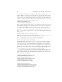
3.14.2 Vertical bar notations
The amsmath package provides commands \lvert, \rvert, \lVert, \rVert
(compare \langle, \rangle) to address the problem of overloading for the
vert bar character |. This character is currently used in LATEX documents to
represent a wide variety of mathematical objects: the ‘divides’ relation in a
number-theory expression like p|q, or the absolute-value operation |z|, or the
‘such that’ condition in set notation, or the ‘evaluated at’ notation fζ (t)t=0 .
The multiplicity of uses in itself is not so bad; what is bad, however, is that fact
that not all of the uses take the same typographical treatment, and that the
complex discriminatory powers of a knowledgeable reader cannot be replicated
in computer processing of mathematical documents, at least not without a significant cost in processing speed, and even then not without falling somewhat
short of human readers’ abilities. It is recommended therefore that there should
be a one-to-one correspondence in any given document between the vert bar
character | and a selected mathematical notation, and similarly for the doublebar command \|. This immediately rules out the use of | and \| for delimiters,
4. OPERATOR NAMES (AMSOPN, AMSMATH PACKAGES)
17
as in the notations for absolute value or norm, because left and right delimiters
are distinct usages that do not relate in the same way to adjacent symbols; recommended practice is therefore to define suitable commands in the document
preamble for any paired-delimiter use of vert bar symbols:
\newcommand{\abs}[1]{\lvert#1\rvert}
\newcommand{\norm}[1]{\lVert#1\rVert}
whereupon the document would contain \abs{z} to produce |z| and \norm{v}
to produce kvk.
—4—
Operator names (amsopn, amsmath packages)
4.1
Defining new operator names
Math functions such as log, sin, and lim are traditionally typeset in roman type
to make them visually more distinct from one-letter math variables, which are
set in math italic. The more common ones have predefined names, \log, \sin,
\lim, and so forth, but new ones come up all the time in mathematical papers,
so the amsopn package provides a general mechanism for defining new ‘operator
names’. As the amsopn package is loaded internally by the amsmath package,
the following features are available there also. To define a math function \xxx
to work like \sin, you write
\DeclareMathOperator{\xxx}{xxx}
whereupon ensuing uses of \xxx will produce xxx in the proper font and automatically add proper spacing on either side when necessary, so that you get
A xxx B instead of AxxxB. In the second argument of \DeclareMathOperator
(the name text), a pseudo-text mode prevails: the hyphen character - will print
as a text hyphen rather than a minus sign and an asterisk * will print as a raised
text asterisk instead of a centered math star. (Compare a-b*c and a − b ∗ c.)
But otherwise the name text is printed in math mode, so that you can use, e.g.,
subscripts and superscripts there.
If the new operator should have subscripts and superscripts placed in ‘limits’
position above and below as with lim, sup, or max, use the * form of the
\DeclareMathOperator command:
\DeclareMathOperator*{\Lim}{Lim}
A few special operator names are predefined by the amsopn package: \varinjlim, \varprojlim, \varliminf, and \varlimsup:
\varlimsup
lim n→∞ Q(un , un − u) ≤ 0
\varliminf
lim n→∞ |an+1 | / |an | = 0
\varinjlim
\varprojlim
λ ∗
lim
−→(mi ) ≤ 0
lim
←− p∈S(A) Ap ≤ 0
18
4.2
6. THE \BOLDSYMBOL COMMAND (AMSBSY, AMSMATH PACKAGES)
\mod and its relatives
Commands \mod, \bmod, \pmod, \pod are provided by the amsopn package to
deal with the special spacing conventions of “mod” notation. \bmod and \pmod
are available in LATEX, but with the amsopn package the spacing of \pmod will
adjust to a smaller value if it’s used in a non-display-mode formula. \mod
and \pod are variants of \pmod preferred by some authors; \mod omits the
parentheses, whereas \pod omits the “mod” and retains the parentheses.
(4.1)
gcd(n, m mod n);
x≡y
(mod b);
x≡y
mod c;
x≡y
(d)
\gcd(n,m\bmod n);\quad x\equiv y\pmod b
;\quad x\equiv y\mod c;\quad x\equiv y\pod d
—5—
The \text command (amstext, amsmath packages)
The \text command is defined by the amsmath package through a subordinate package amstext (which can also be used independently if desired). The
main use of the command \text is for words or phrases in a display. It is
very similar to the LATEX command \mbox in its effects, but has a couple of
advantages. If you want a word or phrase of text in a subscript, you can type
..._{\text{word or phrase}}, which is slightly easier than the \mbox equivalent: ..._{\mbox{\scriptsize word or phrase}}. The other advantage is
the more descriptive name.
(5.1)
f[xi−1 ,xi ] is monotonic, i = 1, . . . , c + 1
f_{[x_{i-1},x_i]} \text{ is monotonic,}
\quad i = 1,\dots,c+1
—6—
The \boldsymbol command (amsbsy, amsmath packages)
The \boldsymbol and \pmb commands are defined by the amsbsy package (also
loaded by amsmath). The \boldsymbol command is used to obtain bold numbers
and other nonalphabetic symbols, as well as bold Greek letters, which cannot
be made bold via the \mathbf command.1 It can also be used to obtain bold
math italic letters; compare the results of M, \mathbf{M} and \boldsymbol{M}:
M MM.
1 Actually, depending on which font set you use, \mathbf may—inconsistently—work for
cap Greek letters but not for lowercase.
7. INTEGRALS AND SUMS (AMSMATH, AMSINTX PACKAGES)
19
The availability of bold symbols varies on different systems depending on
whether or not suitable fonts are installed. The \boldsymbol command should
usually work fine for the common math symbols at 10pt size or larger, but if you
find that it is not having the desired effect for a particular symbol, you could
either (a) verify that the necessary fonts are available and properly installed;
or (b) use \pmb: “poor man’s bold”, which works by printing multiple copies of
the same symbol with slight offsets.
A∞ + πA0 ∼ A∞ + πA0 ∼ A∞ + π A0
(6.1)
A_\infty + \pi A_0
\sim \mathbf{A}_{\boldsymbol{\infty}} \boldsymbol{+}
\boldsymbol{\pi} \mathbf{A}_{\boldsymbol{0}}
\sim\pmb{A}_{\pmb{\infty}} \pmb{+}\pmb{\pi} \pmb{A}_{\pmb{0}}
—7—
Integrals and sums (amsmath, amsintx packages)
7.1
Multiple integral signs
\iint, \iiint, and \iiiint give multiple integral signs with the spacing between them nicely adjusted, in both text and display style. \idotsint is an
extension of the same idea that gives two integral signs with dots between them.
7.2
Multiline subscripts and superscripts
The \substack command can be used to produce a multiline subscript or superscript: for example
\sum_{\substack{0\le i\le m\\ 0<j<n}} P(i,j)
produces a two-line subscript underneath the sum:
X
(7.1)
P (i, j)
0≤i≤m
0<j<n
A slightly more generalized form is the subarray environment which allows you
to specify that each line should be left-aligned instead of centered, as here:
X
(7.2)
P (i, j)
i∈Λ
0<j<n
\sum_{\begin{subarray}{l}
i\in\Lambda\\ 0<j<n
\end{subarray}}
P(i,j)
20
8. COMMUTATIVE DIAGRAMS (AMSCD PACKAGE)
7.3
The \sideset command
There’s also a command called \sideset, for a rather special purpose: putting
symbols
P at
Q the subscript and superscript corners of a large operator symbol such
as
or . The prime example is the case when you want to put a prime on a
sum symbol. If there are no limits above or below the sum, you could just use
\nolimits: here’s \sum\nolimits’ E_n in display mode:
X0
(7.3)
En
If, however, you want not only the prime but also something below or above the
sum symbol, it’s not so easy—indeed, without \sideset, it would be downright
difficult. With \sideset, you can write
\sideset{}{’}\sum_{n<k,\;\text{$n$ odd}} nE_n
to get
X0
(7.4)
nEn
n<k, n odd
The extra pair of empty braces is explained by the fact that \sideset has
the capability of putting an extra symbol or symbols at each corner of a large
operator; to put an asterisk at each corner of a product symbol, you would type
\sideset{_*^*}{_*^*}\prod
producing
∗ Y∗
(7.5)
7.4
∗
∗
The amsintx package
The amsintx package is an experimental package that provides variants of the
\int and \sum commands to better mark the boundaries of the quantity being
summed or integrated. Some commands for differential notation are also provided. If you are interested in this possibility, run LATEX on the documentation
file amsintx.dtx to get the most up-to-date information on usage.
—8—
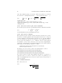
Commutative diagrams (amscd package)
Some commutative diagram commands like the ones in AMS-TEX are available
as a separate package, amscd. For complex commutative diagrams authors will
need to turn to more comprehensive packages like XY-pic (see §C.5), but for
21
9. USING MATH FONTS
simple diagrams without diagonal arrows the amscd commands may be more
convenient. Here is one example.
j
S WΛ ⊗ T −−−−→


y
(S ⊗ T )/I
\begin{CD}
S^{{\mathcal{W}}_\Lambda}\otimes T
@VVV
(S\otimes T)/I
@=
\end{CD}
T


yEnd P
(Z ⊗ T )/J
@>j>>
T\\
@VV{\End P}V\\
(Z\otimes T)/J
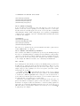
In the CD environment the commands @>>>, @<<<, @VVV, and @AAA give respectively right, left, down, and up arrows. For the horizontal arrows, material
between the first and second > or < symbols will be typeset as a superscript,
and material between the second and third will be typeset as a subscript. Similarly, material between the first and second or second and third As or Vs of
vertical arrows will be typeset as left or right “sidescripts”.
—9—
Using math fonts
9.1
Introduction
For more comprehensive information on font use in LATEX, see the LATEX font
guide (fntguide.tex) or The LATEX Companion [3]. Many users of AMS-LATEX
also obtain an auxiliary collection of math fonts known as ‘AMSFonts’. The basic set of math font commands in LATEX includes \mathbf, \mathrm, \mathcal,
\mathsf, \mathtt, \mathit. Additional math alphabet commands are available
through the packages amsfonts and eucal, if the requisite fonts are installed
on your system (see §C.2).
9.2
Recommended use of math font commands
If you find yourself employing math font commands frequently in your document,
you might wish that they had shorter names, such as \mb instead of \mathbf.
Of course, there is nothing to keep you from providing such abbreviations for
yourself by suitable \newcommand statements. But for LATEX to provide shorter
names would actually be a disservice to authors, as that would obscure a much
better alternative: defining custom command names derived from the names of
the underlying mathematical objects, rather than from the names of the fonts
used to distinguish the objects. For example, if you are using bold to indicate
vectors, then you will be better served in the long run if you define a ‘vector’
command instead of a ‘math-bold’ command:
22
10. THEOREMS AND RELATED STRUCTURES
\newcommand{\vec}[1]{\mathbf{#1}}
whereupon1 you can write \vec{a} + \vec{b} to produce a + b. If you decide
several months down the road that you want to use the bold font for some other
purpose, and mark vectors by a small over-arrow instead, then you can put
the change into effect merely by changing the definition of \vec; otherwise you
would have to replace all occurrences of \mathbf throughout your document,
perhaps even needing to inspect each one to see whether it is indeed an instance
of a vector.
It can also be useful to assign distinct command names for different letters
of a particular font:
\DeclareSymbolFont{AMSb}{U}{msb}{m}{n}% or use amsfonts package
\DeclareMathSymbol{\C}{\mathalpha}{AMSb}{"43}
\DeclareMathSymbol{\R}{\mathalpha}{AMSb}{"52}
These statements would define the commands \C and \R to produce blackboardbold letters from the ‘AMSb’ math symbols font. If you refer often to the
complex numbers or real numbers in your document, you might find this method
more convenient than (let’s say) defining a \field command and writing
\field{C}, \field{R}. But for maximum flexibility and control, define such a
\field command and then define \C and \R in terms of that command:
\usepackage{amsfonts}% to get the \mathbb alphabet
\newcommand{\field}[1]{\mathbb{#1}}
\newcommand{\C}{\field{C}}
\newcommand{\R}{\field{R}}
—10—
Theorems and related structures (amsthm package)
10.1
Introduction
The amsthm package provides an enhanced version of the LATEX command \newtheorem for defining theorem-like environments. The amsthm version of the
\newtheorem command recognizes a \theoremstyle specification (as in Mittelbach’s theorem package) and has a * form for defining unnumbered environments. The amsthm package also defines a proof environment that automatically adds a Q.E.D. symbol at the end. AMS document classes automatically
load the amsthm package, so everything described here applies to them as well.
An example file thmtest.tex is provided in the AMS-LATEX distribution.
1 If you actually tried this example you would discover that the command \vec is already
defined. It produces a different sort of notation for vectors: a small over-arrow ~
x. The solution
is to use \renewcommand (if you expect that you will never need the over-arrow version of the
notation) or to choose a different name for your new vector command.
10. THEOREMS AND RELATED STRUCTURES
10.2
23
The \newtheorem command
In mathematical research articles and books, theorems and proofs are among the
most common elements, but authors also use many others that fall in the same
general class: lemmas, propositions, axioms, corollaries, conjectures, definitions,
remarks,, cases, steps, and so forth. As these elements form a slice of the text
stream with well-defined boundaries, they are naturally handled in LATEX as
environments. But LATEX document classes normally do not provide predefined
environments for theorem-like elements because (a) that would make it difficult
for authors to exercise the necessary control over the automatic numbering,
and (b) the variety of such elements is so wide that it’s just not possible for a
document class to provide every one that will ever be needed. Instead there is
a command \newtheorem, similar to \newenvironment in effect, that makes it
easy for authors to set up the elements required for a particular document.
The \newtheorem command has two mandatory arguments; the first one is
the environment name that the author would like to use for this element; the
second one is the heading text. For example,
\newtheorem{lem}{Lemma}
means that instances in the document of
\begin{lem} Text text ... \end{lem}
will produce
Lemma 1. Text text . . .
where the heading consists of the specified text ‘Lemma’ and an automatically
generated number and punctuation.
If \newtheorem* is used instead of \newtheorem in the above example, there
will not be any automatic numbers generated for any of the lemmas in the
document. This form of the command can be useful if you have only one lemma
and don’t want it to be numbered; more often, though, it is used to produce
a special named variant of one of the common theorem types. For example, if
you have a lemma whose name should be ‘Klein’s Lemma’ instead of ‘Lemma’
+ number, then the statement
\newtheorem*{KL}{Klein’s Lemma}
would allow you to write
\begin{KL} Text text ... \end{KL}
and get the desired output.
10.3
Numbering modifications
In addition to the two mandatory arguments, \newtheorem has two mutually
exclusive optional arguments. These affect the sequencing and hierarchy of the
numbering.
24
10. THEOREMS AND RELATED STRUCTURES
By default each kind of theorem-like environment is numbered independently. Thus if you have three lemmas and two theorems interspersed, they
will be numbered something like this: Lemma 1, Lemma 2, Theorem 1, Lemma
3, Theorem 2. If you want lemmas and theorems to share the same numbering
sequence—Lemma 1, Lemma 2, Theorem 3, Lemma 4, Theorem 5—then you
should indicate the desired relationship as follows:
\newtheorem{thm}{Theorem}
\newtheorem{lem}[thm]{Lemma}
The optional argument [thm] in the second statement means that the lem
environment should share the thm numbering sequence instead of having its
own independent sequence.
To have a theorem-like environment numbered subordinately within a sectional unit—e.g., to get propositions numbered Proposition 2.1, Proposition 2.2,
and so on in Section 2—put the name of the parent unit in square brackets in
final position:
\newtheorem{prop}{Proposition}[section]
With the optional argument [section], the prop counter will be reset to 0
whenever the parent counter section is incremented.
10.4
Changing styles for theorem-like environments
10.4.1 The \theoremstyle command
The amsthm package supports the notion of a current theorem style, which determines what will be produced by a given \newtheorem command. The three
theorem styles provided—plain, definition, and remark—receive different typographical treatment that gives them visual emphasis corresponding to their
relative importance. The details of this typographical treatment may vary depending on the document class, but typically the plain style produces italic
body text, while the other two styles produce roman body text.
To create new theorem-like environments in the different styles, divide your
\newtheorem commands into groups and preface each group with the appropriate \theoremstyle. If no \theoremstyle command is given, the style used
will be plain. Some examples:
\theoremstyle{plain}% default
\newtheorem{thm}{Theorem}[section]
\newtheorem{lem}[thm]{Lemma}
\newtheorem{prop}[thm]{Proposition}
\newtheorem*{cor}{Corollary}
\newtheorem*{KL}{Klein’s Lemma}
\theoremstyle{definition}
\newtheorem{defn}{Definition}[section]
\newtheorem{conj}{Conjecture}[section]
\newtheorem{exmp}{Example}[section]
10. THEOREMS AND RELATED STRUCTURES
25
\theoremstyle{remark}
\newtheorem*{rem}{Remark}
\newtheorem*{note}{Note}
\newtheorem{case}{Case}
10.4.2
Number swapping
A not uncommon style variation for theorem heads is to have the theorem
number on the left, at the beginning of the heading, instead of on the right.
As this variation is usually applied across the board regardless of individual
\theoremstyle changes, number-swapping is done by placing a \swapnumbers
command at the beginning of the list of \newtheorem statements that should
be affected. For example:
\swapnumbers
\theoremstyle{plain}
\newtheorem{thm}{Theorem}
\theoremstyle{remark}
\newtheorem{rem}{Remark}
After the above declarations, theorem and remark heads will be printed in the
form 1.4 Theorem., 9.1. Remark.
10.4.3 Further customization possibilities
More extensive customization capabilities are provided by the amsthm package in
the form of a \newtheoremstyle command and a mechanism for using package
options to load custom theoremstyle definitions. As these capabilities are somewhat beyond the needs of the average user, discussion of the details is consigned
to the example file thmtest.tex and to the commentary in amsthm.dtx.
10.5
Proofs
A predefined proof environment provided by the amsthm package produces the
heading “Proof” with appropriate spacing and punctuation. The proof environment is primarily intended for short proofs, no more than a page or two in
length; longer proofs are usually better done as a separate \section or \subsection in your document.
A ‘Q.E.D.’ symbol, , is automatically appended at the end of a proof
environment. To substitute a different end-of-proof symbol, use \renewcommand
to redefine the command \qedsymbol. For a long proof done as a subsection or
section instead of with the proof environment, you can obtain the symbol and
the usual amount of preceding space by using \qed.
Placement of the Q.E.D. symbol can be problematic if the last part of a
proof environment is a displayed equation or list environment or something of
that nature. Adequate results can sometimes be obtained by using \qed at the
appropriate spot and then undefining \qed just before the end of the proof.
(The effect will be automatically localized to the current proof by normal LATEX
scoping rules.) For example:
26
10. THEOREMS AND RELATED STRUCTURES
\begin{proof}
...
\begin{equation}
G(t)=L\gamma!\,t^{-\gamma}+t^{-\delta}\eta(t) \qed
\end{equation}
\renewcommand{\qed}{}\end{proof}
An optional argument of the proof environment allows you to substitute a
different name for the standard “Proof”. If you want the proof heading to be,
say, “Proof of the Main Theorem”, then write
\begin{proof}[Proof of the Main Theorem]
Appendix A. INSTALLATION INSTRUCTIONS
27
—Appendix A—
Installation instructions
A.1
Introduction
To use version 1.2 of AMS-LATEX it is necessary for you to have a recent version
of LATEX (June 1994 or later, ‘LATEX 2ε ’). If you’re not sure about the version,
look at the startup message that is printed on screen and in the TEX log when
you run LATEX. It should mention the LATEX version number and date somewhere
in the first ten lines. If your version of LATEX is older than June 1994, we
suggest getting the latest version from the Comprehensive TEX Archive Network
(CTAN), directory tex-archive/macros/latex, ftp addresses ftp.shsu.edu
(US), ftp.dante.de (Germany), or ftp.tex.ac.uk (UK). If ftp file transfer is
not an option for you, contact the source from which you originally obtained
LATEX.
A.2
Putting files in a suitable place on your system
See the READ.ME file for possible updates about installation procedures.
There are two ‘areas’ (directories or folders) on your system that are involved
in installing AMS-LATEX: an AMS-LATEX source files area, and a LATEX input
files area. All files in the inputs subdirectory of the AMS-LATEX distribution
should be placed in the LATEX input directory or folder on your system. Consult
your TEX documentation if you don’t know where this is. (You could also try
looking for the file article.cls; the place where you find it is almost surely
your LATEX input files area.)
All other files in the AMS-LATEX distribution (the ones in the math and
classes subdirectories) can be placed in an AMS-LATEX source files area; if
you are installing AMS-LATEX for the first time, create a new folder or directory
for this purpose.
A.3
Testing
For a quick test of the installation, try printing the test file subeqn.tex. For
more extensive tests print the AMS-LATEX user’s guide (amsldoc.tex) or testmath.tex.
A.4
Extra math fonts
For information on the AMSFonts collection, a set of extra math fonts that
supplements the standard set of LATEX math fonts, see §C.2.
A.5
Memory requirements
TEX divides up the memory available to it into various categories. On most
systems the sizes of these categories are fixed at the beginning of a TEX run
and cannot dynamically grow to meet unexpected demands. (In fact certain
implementations of TEX have the sizes fixed at the time a format file is created, or even when the TEX program is compiled.) Use of extra packages places
28
Appendix A. INSTALLATION INSTRUCTIONS
burdens on certain memory categories (string pool, hash size, main memory) in
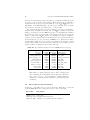
proportion to the total size of the packages. Table A.1 lists the recommended
capacities in various categories for successful use of the AMS-LATEX major documentstyles or the amsmath package. Not all categories are listed; the ones that
appear are the ones where problems tend to occur nowadays.
Note in particular that the base value for string pool needs to be much larger
than the values typically found at the end of a LATEX log. This is because the
string pool capacity reported by TEX in response to a \tracingstats command
is not the base value, but the result of subtracting from the base value the
number of characters in TEX’s built-in error messages, the names of primitive
control sequences, and the names of all additional control sequences defined in
the format file (in our case, the whole of LATEX), not to mention font names
and file names. Thus the reported value only measures the amount of string
capacity that remains to the user after the format file is loaded. The reported
value for number of strings is reduced in the same way.
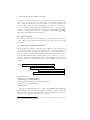
Table A.1. Recommended values for selected TEX memory categories
Category
strings
string characters
macro string pool∗
main memory
control sequences
font information
number of fonts
input buffer
save stack
∗
A.6
Capacity
Adequate Generous
5 000
30 000
80 000
300 000
50 000
270 000
80 000
250 000
5 000
20 000
60 000
300 000
128
256
1 000
5 000
2 000
10 000
WEB variable
max_strings
pool_size
string_vacancies
main_mem
hash_size
font_mem_size
font_max
buf_size
save_size
The number of string characters left for macro packages and
user commands, after all primitives and built-in error messages
have been loaded—i.e., the total number of string characters
available for a format file and individual documents using that
format file.
Files included in this distribution
As files are occasionally added or removed from the distribution, you should
check the READ.ME file if you want the most up-to-date possible list.
File name
Description
amsldoc.tex user’s guide
amslatex.faq frequently asked questions
amslatex.bug description of bug fixes and other changes
Appendix B. ERROR MESSAGES AND OUTPUT PROBLEMS
diff12.tex
technote.tex
amslatex.ins
testmath.tex
subeqn.tex
amsbsy.dtx
amscd.dtx
amsgen.dtx
amsintx.dtx
amsmath.dtx
amsopn.dtx
amstext.dtx
amsxtra.dtx
amstex.sty
amsdtx.dtx
29
description of differences between versions 1.1 and 1.2
some technical notes
installation file
test file for general math features
test file for ‘subequations’ environment
for \boldsymbol and \pmb
for commutative diagrams
auxiliary file
alternative command syntax for integrals and sums
equations and other math
operator names
\text command
misc rarely used commands
frozen version of old amstex package
document class for printing AMS .dtx files
instr-l.tex instructions for using AMS document classes
amsclass.dtx Source for amsart, amsbook, and amsproc document
classes
amsthm.dtx
provides \theoremstyle, \newtheorem*
upref.dtx
makes \ref always produce roman/upright numbers
thmtest.tex Test file for the amsthm package
amsalpha.bst Bibliography style for BibTEX
amsplain.bst Bibliography style for BibTEX
mrabbrev.bib BibTEX abbreviations for MR journal names
—Appendix B—
Error messages and output problems
B.1
General remarks
This is a supplement to Chapter 8 of the LATEX manual [5] (first edition: Chapter 6). For the reader’s convenience, the set of error messages discussed here
overlaps somewhat with the set in that chapter, but please be aware that we
don’t provide exhaustive coverage here. The error messages are arranged in
alphabetical order, disregarding unimportant text such as ! LaTeX Error: at
the beginning, and nonalphabetical characters such as \. Where examples are
given, we show also the help messages that appear on screen when you respond
to an error message prompt by entering h.
There is also a section discussing some output errors, i.e., instances where
the printed document has something wrong but there was no LATEX error during
typesetting.
30
B.2
Appendix B. ERROR MESSAGES AND OUTPUT PROBLEMS
Error messages
\begin{split} won’t work here.
Example:
! Package amsmath Error: \begin{split} won’t work here.
...
l.8 \begin{split}
? h
\Did you forget a preceding \begin{equation}?
If not, perhaps the ‘aligned’ environment is what you want.
?
Explanation: The split environment does not construct a stand-alone displayed
equation; it needs to be used within some other environment such as equation
or gather.
Extra & on this line
Example:
! Package amsmath Error: Extra & on this line.
See the amsmath package documentation for explanation.
Type H <return> for immediate help.
...
l.9 \end{alignat}
? h
\An extra & here is so disastrous that you should probably exit
and fix things up.
?
Explanation: In an alignat structure the number of alignment points per line
is dictated by the numeric argument given after \begin{alignat}. If you use
more alignment points in a line it is assumed that you accidentally left out a
newline command \\ and the above error is issued.
Font OMX/cmex/m/n/7=cmex7 not loadable ...
Example:
! Font OMX/cmex/m/n/7=cmex7 not loadable: Metric (TFM) file not found.
<to be read again>
relax
l.8 $a
b+b^2$
? h
Appendix B. ERROR MESSAGES AND OUTPUT PROBLEMS
31
I wasn’t able to read the size data for this font,
so I will ignore the font specification.
[Wizards can fix TFM files using TFtoPL/PLtoTF.]
You might try inserting a different font spec;
e.g., type ‘I\font<same font id>=<substitute font name>’.
?
Explanation: Certain extra sizes of some Computer Modern fonts that were
formerly available mainly through the AMSFonts distribution are considered
part of standard LATEX (as of June 1994): cmex7–9, cmmib5–9, and cmbsy5–9.
If these extra sizes are missing on your system, you should try first to get them
from the source where you obtained LATEX. If that fails, you could try getting
the fonts from CTAN (e.g., in the form of Metafont source files, directory /texarchive/fonts/latex/mf, or in PostScript Type 1 format, directory /texarchive/fonts/cm/ps-type1/bakoma).
If the font name begins with cmex, there is a special option cmex10 for
the amsmath package that provides a temporary workaround. I.e., change the
\usepackage to
\usepackage[cmex10]{amsmath}
This will force the use of the 10-point size of the cmex font in all cases. Depending on the contents of your document this may be adequate.
Foreign command \over; use \frac or \genfrac instead
Example:
! Package amsmath Error: Foreign command: \over; use \frac or \genfrac instead.
See the amsmath package documentation for explanation.
Type H <return> for immediate help.
...
l.49 Fractions ${1\over
2}$ and
?
Explanation: The primitive generalized fraction commands of TEX are disallowed
by the amsmath package because their syntax is foreign to LATEX. The substitutes
\frac and \genfrac are provided instead. See §3.11.1 for further information.
Math formula deleted: Insufficient extension fonts
Example:
! Math formula deleted: Insufficient extension fonts.
l.8 $ab+b^2$
?
32
Appendix B. ERROR MESSAGES AND OUTPUT PROBLEMS
Explanation: This usually follows a previous error Font ... not loadable; see
the discussion of that error (above) for solutions.
Missing number, treated as zero
Example:
! Missing number, treated as zero.
<to be read again>
a
l.100 \end{alignat}
? h
A number should have been here; I inserted ‘0’.
(If you can’t figure out why I needed to see a number,
look up ‘weird error’ in the index to The TeXbook.)
?
Explanation: There are many possibilities that can lead to this error. However,
one possibility that is relevant for the amsmath is that you forgot to give the
number argument of an alignat environment, as in:
\begin{alignat}
a& =b&
c& =d\\
a’& =b’&
c’& =d’
\end{alignat}
where the first line should read instead
\begin{alignat}{2}
Another possibility is that you have a left bracket character [ following a
linebreak command \\ in a multiline construction such as array, tabular, or
eqnarray. This will be interpreted by LATEX as the beginning of an ‘additional
vertical space’ request [5, §C.1.6], even if it occurs on the following line and is
intended to be part of the contents. For example
\begin{array}
a+b\\
[f,g]\\
m+n
\end{array}
To prevent the error message in such a case, you can add braces as discussed in
the LATEX manual [5, §C.1.1]:
\begin{array}
a+b\\
{[f,g]}\\
m+n
\end{array}
Appendix B. ERROR MESSAGES AND OUTPUT PROBLEMS
33
Missing \right. inserted
Example:
! Missing \right. inserted.
<inserted text>
\right .
l.10 \end{multline}
? h
I’ve inserted something that you may have forgotten.
(See the <inserted text> above.)
With luck, this will get me unwedged. But if you
really didn’t forget anything, try typing ‘2’ now; then
my insertion and my current dilemma will both disappear.
Explanation: This error typically arises when you try to insert a linebreak inside
a \left-\right pair of delimiters in a multline or split environment:
\begin{multline}
AAA\left(BBB\\
CCC\right)
\end{multline}
There are two possible solutions: (1) instead of using \left and \right, use
‘big’ delimiters of fixed size (\bigl \bigr \biggl \biggr . . . ; see §3.14.1); or
(2) use null delimiters to break up the \left-\right pair into parts for each
line:
AAA\left(BBB\right.\\
\left.CCC\right)
The latter solution may result in mismatched delimiter sizes; ensuring that they
match requires using \vphantom in the line that has the smaller delimiter (or
possibly \smash in the line that has the larger delimiter). In the argument of
\vphantom put a copy of the tallest element that occurs in the other line, e.g.,
xxx \left(\int_t yyy\right.\\
\left.\vphantom{\int_t} zzz ... \right)
Paragraph ended before \xxx was complete
Example:
Runaway argument?
! Paragraph ended before \equation was complete.
<to be read again>
\par
l.100
34
Appendix B. ERROR MESSAGES AND OUTPUT PROBLEMS
? h
I suspect you’ve forgotten a ‘}’, causing me to apply this
control sequence to too much text. How can we recover?
My plan is to forget the whole thing and hope for the best.
?
Explanation: This might be produced by a misspelling in the \end{equation}
command, e.g.,
\begin{equation}
...
\end{equatin}
or by using abbreviations such as \beq and \eeq for \begin{equation} and
\end{equation}:
\beq
...
\eeq
That kind of abbreviation works in ordinary LATEX but for technical reasons
it does not work with any of the displayed equation environments (gather,
align, split, equation, etc.) when the amsmath package is used. Work to
re-enable the use of such abbreviations is under way, but nontrivial technical
complications are involved (cf. technote.tex).
Runaway argument?
See the discussion for the error message Paragraph ended before \xxx
was complete.
Unknown option ‘xxx’ for package ‘yyy’
Example:
! LaTeX Error: Unknown option ‘intlim’ for package ‘amsmath’.
...
? h
The option ‘intlim’ was not declared in package ‘amsmath’, perhaps you
misspelled its name. Try typing <return> to proceed.
?
Explanation: This means that you misspelled the option name, or the package
simply does not have an option that you expected it to have. Consult the
documentation for the given package.
B.3
Wrong output
B.3.1 Section numbers 0.1, 5.1, 8.1 instead of 1, 2, 3
This most likely means that you have the arguments for \numberwithin in
reverse order:
Appendix C. OTHER USEFUL ITEMS FOR MATHEMATICAL DOCUMENTS
35
\numberwith{section}{equation}
That means ‘print the section number as equation number.section number and
reset to 1 every time an equation occurs’ when what you probably wanted was
the inverse
\numberwith{equation}{section}
B.3.2
The \numberwithin command had no effect on equation numbers
Are you looking at the first section in your document? Check the section numbers elsewhere to see if the problem is the one described in §B.3.1.
B.3.3
Double accent command failed to position the second accent
properly
The capitalization of the command names is important. Check whether all of
the accent commands are capitalized. Compare
ˆ ˆ ˆ
Aˆ Aˆ Aˆ
\[\hat{\hat{A}}\quad\Hat{\hat{A}}\quad\Hat{\Hat{A}}\]
B.3.4 The \boldsymbol command didn’t work
This probably means that the font necessary to produce a bold version of the
symbol in question is not available on your system or not installed in a way that
LATEX can use it. For example, bold versions of the AMS extra symbol fonts
msam and msbm do not currently exist, so \boldsymbol{\square} will merely
produce the same result as \square alone.
Also, the weight of the fonts cmmib and cmbsy is ‘bold’ rather than ‘bold
extended’ as for cmbx. Depending on the symbol in question and the resolution
of your printer (or previewer), a symbol that was taken from one of those two
bold symbol fonts might be nearly indistinguishable from the non-bold version.
—Appendix C—
Other useful items for mathematical documents
C.1
AMS documentclasses (amsart, amsbook, amsproc)
The American Mathematical Society provides custom AMS-LATEX document
classes for AMS journals and book series. These may obtained by anonymous
FTP from the e-MATH system e-math.ams.org, directory, in the authorinfo area. (Note that directory structures may occasionally change; if you
have trouble locating files you need, please contact AMS Technical Support; see
Appendix E.) Specific and generic classes can be requested by e-mail to [email protected] or ordered on floppy disk through the AMS Customer
Services Department at [email protected] or 800-321-4267.
36
C.2
Appendix D. WHERE TO FIND OTHER INFORMATION
Extra math fonts (the AMSFonts collection)
The ‘AMSFonts’ font collection is a set of extra math fonts that supplements the
standard set of LATEX math fonts. It includes LATEX packages called amsfonts
and amssymb that make it easy to use the extra fonts in a LATEX document.
If you don’t have the AMSFonts collection already on your system, and would
like to use some of the symbols in it, it can be obtained by anonymous FTP
from CTAN (see §A.1) or from the e-MATH system at e-math.ams.org. It
can also be ordered on disk from the AMS Customer Services Department at
[email protected] or 800-321-4267.
C.3
Syntax checking (the syntonly package)
If you are working on a relatively slow computer system you might want to try
the syntonly package. This makes LATEX skim through your document only
checking for proper syntax and usage of the commands, but not producing any
printed pages. As LATEX runs quite a bit faster under those conditions, for
early error-checking runs of a document this can save you valuable time. The
syntonly package is a standard LATEX package so you should find it already on
your system; to use it, write
\usepackage{syntonly}
\syntaxonly
When you want to produce pages, comment out the second line by adding a
percent character:
%\syntaxonly
C.4
Verbatim and comments (the verbatim package)
The verbatim package is another standard LATEX package, like syntonly. In
addition to some minor enhancements for the verbatim environment, it provides
a comment environment that skips everything between \begin{comment} and
the next \end{comment}. A command \verbatiminput is also provided for
typesetting a whole file in verbatim style.
C.5
Commutative diagrams and other diagrams (packages diagram,
xypic, pstricks)
The amscd package for commutative diagrams that is included in the AMSLATEX distribution is quite limited. The following packages are worth investigation for authors who need more powerful diagram features: diagram, xypic,
pstricks. These are available by anonymous FTP from CTAN (see §A.1). The
diagram package, by Michael Barr, focuses on commutative diagrams and is
thus smaller than the others; it uses LATEX arrows as produced by \vector
for diagram construction. The xypic package, by Kristoffer Rose, is a more
general diagram package; it requires special arrow fonts (included in the xypic
distribution) or PostScript capabilities in your system. The pstricks package,
by Timothy van Zandt, also provides general diagram object commands; it is
strictly for PostScript use, as the name implies.
Appendix E. GETTING HELP
37
—Appendix D—
Where to find other information
D.1
Technical notes
The file technote.tex contains some remarks on miscellaneous technical questions related to AMS-LATEX; they are relegated to a separate document because
they are unlikely to be of interest to most users.
D.2
Differences between AMS-LATEX version 1.1 and AMS-LATEX
version 1.2
Version 1.2 of AMS-LATEX fills in some gaps and corrects some mistakes in the
AMS-LATEX 1.1 feature set. The significant differences, from a user’s perspective, are described in the document diff12.tex.
—Appendix E—
Getting help
Questions or comments regarding the AMS-LATEX package should be sent to:
American Mathematical Society
Technical Support
Electronic Products and Services
P. O. Box 6248
Providence, RI 02940
Phone: 800-321-4AMS (321-4267) or 401-455-4080
Internet: [email protected]
If you are reporting a problem you should include the following information to
make proper investigation possible:
1. The source file where the problem occurred, preferably reduced to minimum size by removing any material that can be removed without affecting
the observed problem.
2. A LATEX log file showing the error message (if applicable) and the version
numbers of the document class and option files being used.
E.1
Further information
Information about obtaining AMSFonts or other TEX-related software from the
AMS Internet archive e-math.ams.org can be obtained by sending a request
through electronic mail to: [email protected].
38
BIBLIOGRAPHY
Information about obtaining AMS-LATEX on diskette from the AMS is available from:
American Mathematical Society
Customer Services
P. O. Box 6248
Providence, RI 02940
Phone: 800-321-4AMS (321-4267) or 401-455-4000
Internet: [email protected]
The TEX Users Group is a nonprofit organization that publishes a journal
(TUGboat ), holds meetings, and serves as a clearing-house of general information about TEX and TEX-related software.
TEX Users Group
P. O. Box 869
Santa Barbara, CA 93102-0869
Phone: (805) 963-1338
Internet: [email protected]
Membership in the TEX Users Group is a good way to support continued development of free TEX-related software. There are also many local TEX user
groups in other countries; information about contacting a local user group can
be gotten from the TEX Users Group.
There is a Usenet newsgroup called comp.text.tex that is a fairly good
source of information about LATEX and TEX in general. If you don’t know
about reading newsgroups, check with your local system administrator to see if
newsgroup service is available at your site.
Bibliography
[1] AMSFonts version 2.2—user’s guide, Amer. Math. Soc., Providence, RI,
1994; distributed with the AMSFonts package.
[2] Instructions for preparation of papers and monographs—AMS-LATEX, Amer.
Math. Soc., Providence, RI, 1994.
[3] Michel Goossens, Frank Mittelbach, and Alexander Samarin, The LATEX
companion, Addison-Wesley, Reading, MA, 1994.
[4] Donald E. Knuth, The TEXbook, Addison-Wesley, Reading, MA, 1984.
[5] Leslie Lamport, LATEX: A document preparation system, 2nd revised ed.,
Addison-Wesley, Reading, MA, 1994.
[6] Frank Mittelbach and Rainer Sch¨
opf, The new font family selection—user
interface to standard LATEX, TUGboat 11, no. 2 (June 1990), pp. 297–305.
[7] Michael Spivak, The joy of TEX, 2nd revised ed., Amer. Math. Soc., Providence, RI, 1990.
Index
\!, 10
\,, 10
\:, 10
\;, 10
\\, 3, 7, 8, 30, 32
\\*, 8
\|, 16
amsmath.dtx, 29
amsopn package, 1, 17, 18
amsopn.dtx, 29
amsplain.bst, 29
amsproc class, 29, 35
amssymb package, 36
AMS-TEX, v
amstex package, 29
amstex.sty, 29
amstext package, 1, 18
amstext.dtx, 29
amsthm package, vi, 1, 22, 24, 25, 29
amsthm.dtx, 25, 29
amsxtra package, 1, 12
amsxtra.dtx, 29
array environment, 9, 10, 32
arrows
extensible, 13
in commutative diagrams, 21
article.cls, 27
\atop, 13
\atopwithdelims, 13
author-info, 35
\above, 13
\abovewithdelims, 13
\accentedsymbol, 1, 12
accents
double, 12
\addtocounter, 9, 10
\addtolength, 3
align environment, 2, 5, 6, 34
alignat environment, 6, 30, 32
aligned environment, 6
\allowdisplaybreaks, 8
allowdisplaybreaks environment,
7
amsalpha.bst, 29
amsart class, 29, 35
amsbook class, 29, 35
amsbsy package, 1, 18
amsbsy.dtx, 29
amscd package, 1, 20, 21, 36
amscd.dtx, 29
amsclass.dtx, 29
amsdtx.dtx, 29
amsfonts package, 21, 36
AMSFonts collection, 21, 31, 36
amsgen.dtx, 29
amsintx package, 1, 19, 20
amsintx.dtx, 20, 29
AMS-LATEX user’s guide, 27
amslatex.bug, 28
amslatex.faq, 28
amslatex.ins, 29
amsldoc.tex, 27, 28
amsmath environment, 32
amsmath package, 1–3, 5, 7, 9–19,
28, 31, 34
BaKoMa fonts, 31
\big, \Big, \bigg, . . . delimiters,
16
\biggl, 33
\biggr, 33
\bigl, 33
\bigr, 33
\binom, 13, 14
binomials, 14
bmatrix environment, 9
\bmod, 18
\boldsymbol, vi, 1, 18, 19, 29, 35
\boxed, 13
\C, 22
cases environment, 7
CD environment, 1, 21
centertags option, 1
\cfrac, 15
39
40
classes, 27
cmbsy, 35
cmbsy5, 31
cmbx, 35
cmex, 31
cmex10, 31
cmex7, 31
cmmib, 35
cmmib5, 31
comment environment, 36
commutative diagrams, 36
comp.text.tex, 38
Comprehensive TEX Archive Network,
see CTAN
continued fractions, 14
CTAN, 27, 36
\dbinom, 14
\ddddot, 12
\dddot, 12
\ddot, 12
\DeclareMathOperator, 1, 17
definition theorem style, 24
delimiters
size adjustments, 15
\dfrac, 13, 14
diagram package, 36
diff12.tex, 29, 37
differential notation, 20
\displaybreak, 7, 8
displayed equations, 2
centering, 2
displaymath environment, 3
\displaystyle, 14
\documentclass, 2
\dot, 12
dots, see ellipsis dots
\dots, 11
\dotsb, 11
\dotsc, 11
\dotsi, 11
\dotsm, 11
e-math.ams.org, 35–37
ellipsis dots
in matrices, 10
INDEX
\end, 11
eqnarray environment, vi, 2, 7, 32
\eqref, 9
equation environment, vi, 2, 3, 5,
30, 34
equation numbers
cross-references, 9
hierarchy, 9
left or right placement, 2
overriding, 3
subordinate numbering, 9
vertical placement, 1
equation* environment, 3
equations, see displayed equations
eucal package, 21
\fbox, 13
\field, 22
fleqn option, 2, 3
fntguide.tex, 21
\frac, 13–15, 31
fractions, 13
\fracwithdelims, 1
FTP, 36
ftp.dante.de, 27
ftp.shsu.edu, 27
ftp.tex.ac.uk, 27
function names, see operator names
gather environment, 5, 30, 34
gathered environment, 6
\genfrac, 13, 14, 31
\Hat, 12
\hat, 12
\hdotsfor, 10
horizontal space
around operator names, 17
in math mode, 10
\idotsint, 19
\iiiint, 19
\iiint, 19
\iint, 19
inputs, 27
installation, 27
41
INDEX
instr-l.tex, 29
\int, 20
integrals, 20
multiple, 19
placement of limits, 2
\intertext, 8
intlimits option, 2
\label, 9
Lamport, Leslie, v
\langle, 16
\left, 15, 16, 33
\leftroot, 12
leqno option, 2
\lim, vi, 1, 17
limits, see subscripts and superscripts
\log, 17
\lVert, 16
\lvert, 16
math, 27
math fonts, 21
bold symbols, 18
math symbols, see math fonts
\mathbf, 18, 21, 22
\mathcal, 21
\mathit, 21
\mathrm, 21
\mathsf, 21
\mathtt, 21
matrices, 9
ellipsis dots, 10
matrix environment, 9
\mbox, 18
\medspace, 10
Metafont source files, 31
Mittelbach, Frank, v
\mod, 18
mrabbrev.bib, 29
msam, 35
msbm, 35
\mspace, 11
multline environment, 3, 5, 33
\multlinegap, 3
namelimits option, 2
\negmedspace, 10
\negthickspace, 10
\negthinspace, 10
\newcommand, 12, 21
\newenvironment, 23
\newtheorem, vi, 1, 22–25
\newtheorem*, 23, 29
\newtheoremstyle, 25
\nobreakdash, 11, 12
nointlimits option, 2
\nolimits, 20
nonamelimits option, 2
nosumlimits option, 2
\notag, 3
\numberwithin, 9, 34, 35
operator names, 17
\over, 13
\overleftarrow, 11
\overleftrightarrow, 11
\overrightarrow, 11
\overset, 13
\overwithdelims, 13
page breaks, 7
\pagebreak, 8
plain theorem style, 24
pmatrix environment, 9
\pmb, 1, 18, 19, 29
\pmod, 18
\pod, 18
PostScript fonts, 31
proof environment, vi, 1, 22, 25
proofs, 23
pstricks package, 36
\qed, 25
\qedsymbol, 25
\qquad, 10
\quad, 10, 11
\R, 22
\raisetag, 7
\rangle, 16
READ.ME, 27, 28
\ref, 1, 9, 29
42
remark theorem style, 24
\renewcommand, 22, 25
reqno option, 2
\right, 15, 16, 33
\rVert, 16
\rvert, 16
\savebox, 12
Sch¨
opf, Rainer, v
\scriptscriptstyle, 14
\scriptstyle, 14
\section, 25
\setcounter, 9, 10
\setlength, 3
\shoveleft, 3
\shoveright, 3
\sideset, 13, 20
\sin, vi, 1, 17
smallmatrix environment, 10
\smash, 15, 33
Spivak, Michael, v
split environment, 2, 5, 30, 33, 34
\square, 35
\stackrel, 13
subarray environment, 19
subeqn.tex, 3, 27, 29
subequations environment, 9
subscripts and superscripts, 13
multi-line, 19
on sums, 20
placement, 1, 2
\subsection, 25
\substack, 19
\sum, 20
sumlimits option, 1, 2
sums, 20
superscripts, see subscripts and superscripts
\swapnumbers, 25
syntonly package, 36
tabular environment, 32
\tag, 3
\tag*, 3
\tbinom, 14
tbtags option, 1
INDEX
technote.tex, 13, 29, 34, 37
testmath.tex, 3, 27, 29
TEX Users Group, 38
\text, 1, 6, 7, 18, 29
text fragments inside math, 8, 18
\textstyle, 14
\tfrac, 13, 14
\theequation, 8, 9
theorem package, 22
theorems, 23
numbering, 23
\theoremstyle, 22, 24, 25, 29
\thickspace, 10
\thinspace, 10
thmtest.tex, 22, 25, 29
TUGboat, 38
\underleftarrow, 11
\underleftrightarrow, 11
\underrightarrow, 11
\underset, 13
upref package, 1
upref.dtx, 29
\uproot, 12
\usepackage, 1, 2, 31
\value, 9
\varinjlim, 17
\varliminf, 17
\varlimsup, 17
\varprojlim, 17
\vec, 22
\vector, 36
verbatim environment, 36
verbatim package, 36
\verbatiminput, 36
Vmatrix environment, 9
vmatrix environment, 9
\vphantom, 33
\xleftarrow, 13
\xrightarrow, 13
\xxx, 34
xypic package, 36