Download PC-Radar User Guide

PC-Radar User Guide
Klaus von der Heide, DJ5HG
1. General
PCradar is a program, which in combination with a PC, a radio-amateur SSB-transmitter including
the antenna, and a corresponding receiver with it's own antenna, realizes a simple low-bandwidth
radar. The program is written in Matlab. It is compiled by the Matlab Compiler.
2. Requirements
(a)
(b)
(c)
(d)
To run the program pcsonar.exe the Matlab Compiler Rumtime (MCR) must be installed.
pcradar.exe runs on all Windows systems later than Win98 and on 32 bit and 64 bit versions.
The soundcard must support the samplerate 48000 (for chirp radar).
Two antennas at sufficient distance such that the direct signal is received not larger than about
60 dB over the noise.
(e) Radioamateur SSB-transmitter and SSB-receiver.
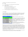
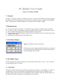
3. The Main Window
Figure 1. The Main window of PCradar.
PCradar starts with a simple window which allows selection of
the desired experiment. Pushing the help button to the right of
an option displays specific help.
4. The Radar Types
PCradar supports two different radar types. A mouseclick on the button chirp or code opens the
corresponding parameter window
4.1. Chirp Radar
This type of radar transmits a tone with raising frequency starting at f1 and ending at f2. This is a
socalled chirp. The received signal has a propagation delay proportional to the distance of the
reflecting target. Therefore the reflected signal has a lower frequency than the actual frequency of
the chirp. The frequency difference is proportional to the distance.
Figure 2. The parameter window of Chirp Radar
The range of the radar can arbitrarily be set.
The resolution of the chirpradar is proportional to the
difference of both edge frequencies. But the edge
frequencies should not exceed the bandwidth of the
SSB-transmitter and receiver. Therefore, the default of
500 Hz and 2500 Hz usually is a good choice.
The relaxation factor controls the time constant of the
order-1-IIR-filter of the display. The integration time is
about 0.1 / (relaxation factor). A value 0.1
guarantees a fast display of changes. A value 0.001 averages the echoes over about one minute. So
noise is well suppressed.
Both radar types need an identical time basis at the sound output and the sound input. I.e. the
samplerates (in the case of chirp radar 48000) must exactly be the same. If these samplerates differ
even slightly, then the echos move slowly along the distance scale. This surely will happen, if
different soundcards are used for output and input. This effect can be compensated by an appropiate
value of the in/out-ratio parameter. If for example the output samplerate is larger than the input
samplerate the in/out-ratio 1.003, then the output signal is resampled by the nominal samplerate
divided by 1.003. If this incorrect signal is sent by the incorrect sound output, the sound input sees
it as a correct signal. Samplerate errors of soundcards usually are very large (0.99 ... 1.01).
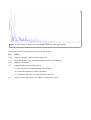
Figure 3. The display of echoes over the distance. In this case the sonar application with speaker
and microphone as the transmitter and receiver. The distances then are scaled by the ratio of (speed
of sound) / (speed of light). The figure shows the author's office. Everything beyond 6m is from
multiple reflections.
The display can be controlled by some specific key-presses:
Key
Effect
c, C
clears the history of the correlation signals (restart of the display)
h, H
displays a help text
t, T
toggles the horizontal scale between:
(1) time delay between transmission and reception
(2) backscatter distance in radar application
(3) backscatter distance in sonar application (air 20 C)
s, S
stops the radar application. The figures remain on the screen.
4.2 Code Radar
The code radar transmits a sequence of bits in PSK-modulation at 2000 Baud on a carrier of about
1500 Hz. The bitsequence is repeated seamlessly. The length of the sequence is as large that the
period is larger than the propagation delay of backscatter from a long path (2×30000 km). The
binary pattern is a Hadamardcode, which has minimal autocorrelation.
Figure 4. The parameter window of code radar.
The relaxation factor controls the time constant of the
order-1-IIR-filter of the display. The integration time
is about 0.1 / (relaxation factor). A value 0.1
guarantees a fast display of changes. A value 0.001
averages the echoes over about one minute. So noise
is well suppressed.
The samplerate may be chosen as 8000, 16000,
32000, 48000. Choose a rate at which the echoes do
not move over the distance axis.
Both radar types need an identical time basis at the sound output and the sound input. I.e. the
samplerates must exactly be the same. If these samplerate differ even slightly, then the echos move
slowly along the distance scale. This surely will happen, if different soundcards are used for output
and input. This effect can be compensated by an appropiate value of the in/out-ratio parameter. If
for example the output samplerate is larger than the input samplerate by the in/out-ratio 1.003, then
the output signal is resampled by the nominal samplerate divided by 1.003. If this incorrect signal is
sent by the incorrect sound output the sound input sees it as a correct signal. Samplerate errors of
soundcards usually are very large (0.99 ... 1.01).
If some other station uses PCsonar on the same frequency, you can avoid interference by selection
of a different Hadamard code by the parameter code number (CDMA-technique).
Figure 5. The display of echoes over the distance (here the sonar application).
The display can be controlled by some specific key-presses:
Key
Effect
b, B
pops up a display with the actual binary code
c, C
clears the history of the correlation signals (restart of the display)
h, H
displays a help text
t, T
toggles the horizontal scale between:
(1) time delay between transmission and reception
(2) backscatter distance in radar application
(3) backscatter distance in sonar application (air 20 C)
s, S
stops the radar application. The figures remain on the screen.
5. The Mathematics of the Radar
5.1 The Chirp Radar
The Chirp
The phase of a constant carrier is a linear function of time t :
The phase of a linear chirp is a quadratic function of time t :
The generated complex signal is given by
φ=ωt
φ = ω t + q t2
x = exp(i φ)
The Transmitted and the Received Signal
Only the real part of the generated signal x is sent.
The signal propagates at the speed of light c.
The length of the propagation path may be s.
Then the signal is received after a pathdelay of Δt=s/c.
The imaginary part of the received signal is reconstructed from the received real part, but with
negative sign. This complex signal is the complex conjugate of x(t – Δt):
y = conj( x(t – Δt) ).
The Chirp-Radar Algorithm
z = x y = exp(i (ω t + q t2) ) exp(–i (ω (t – Δt) + q (t – Δt)2) ) = exp(i (ω Δt – q Δt2 + 2q Δt t ) ).
Separation of the constant factor
leads to
a = exp(i (ω Δt – q Δt2 ) ) and replacement of Δt by Δt=s/c
z = a exp(i Ω t ) with Ω = 2q s/c .
Thus z is a wave of angular velocity Ω, which is proportional to the length of the propagation path
s . Therefore, the spectrum of z indicates all targets by corresponding peaks. The angular velocities
of the spectrum only must be mapped to distances by s = c Ω / (2q) .
The Implementation
The signal processing loop of the Matlab program directly follows the above algorithm. But of
course, it adds some technical features for
(a) communication with the soundcard
(b) calibration of the timing between input and output
(c) noise reduction by a highpass filter
(d) noise reduction by a pulse-blanker
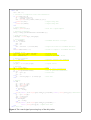
(e) graphical output
The main parts of the above algoritm are highlighted in the following signal processing loop of the
program by yellow background.
Legend to Figure 6. The colors of the words mean:
while
key words of the Matlab languge
filter
standard functions of Matlab including the Signal Processing Toolbox
% FFT
comments
Program-specific objects and variables are in black. They are declared outside of this central loop.
while run
cnt = cnt + 1;
% correction of samplerate error and transmission
if abs(1-fsf)>10^-10
zz = z:fsf:n+1-10^-10;
z
= zz(end) + fsf - n;
txs = spline(1:n+1,[txdat; txdat(1)],zz)';
putdata(ao,txs);
% output chirp data
else
putdata(ao,txdat);
% output chirp data
end
% input sampling
rxsig = getdata(ai,n)';
% wait for n input samples
% distance calibration
rxsig = rxsig([shiftindex:end 1:shiftindex-1]);
% high pass filter
[rxh,hps] = filter(hp,1,rxsig,hps);
% noise blanker
st = std(rxh);
if clr || cnt<10
mst = st;
clr = 0;
else
mst = relax*st + (1-relax)*mst;
end
rxh(abs(rxh)>3*mst) = 0;
% standard deviation of signal
% simple IIR filter for standard deviation
% blank all samples > 3*standard deviation
% Hilbert filter
[rxi,hst] = filter(bh,1,rxh,hst);
rxa = [rst rxh(1:nd)] - 1i*rxi;
rst = rxh(nd+1:n);
% Hilbert filter
% analytical signal
% state of real shift filter
% shift to baseband
v
= txa.*rxa;
% spectral rotation into baseband
% filter
[w,lps] = filter(b,a,v,lps);
% lowpass filter
% spectrum
sp = fft(w.*hgn);
yd = abs(sp(1:mi));
yr = abs(sp(end-mi+1:end));
if clr
ym = yd + yr;
clr = 0;
else
ym = relax*(yd+yr) + (1-relax)*ym;
end
% FFT
% echo of actual transmission
% echo of previous transmission
% actual echo
% mean echo
% display
if mde
yy = yd + yr - ym;
yy = yy - min(yy);
scl = 1/mean(yy);
mxy = max(yy);
if scl*mxy>5
scl = 5/mxy;
end
set(ls,'XData',(1:2*length(ym))/2*km_pro_bin(modus),'YData',interp(scl*yy,2)) %difference
else
yy = ym - min(ym);
scl = 1/mean(yy);
mxy = max(yy);
if scl*mxy>5
scl = 5/mxy;
end
set(ls,'XData',(1:2*length(ym))/2*km_pro_bin(modus),...
'YData',interp(scl*yy,2)) % update mean echo
end
end % while run
Figure 6. The central signal processing loop of the chirp radar.
5.2. The Code Radar
The code radar determines the pathdelay directly in time domain by measuring the time shift
between transmitted and received binary pattern. The received signal is filtered with the reverse
pattern of the transmitted signal as the filter coefficients. The absolute value of the filter output is
displayed over the time delay (or the radar distance or the sonar distance).
To avoid interference with other stations running PCradar on the same frequency, one of the
following four Hadamard codes can be chosen:
code{1}
0 1 0 1
0 1 0 1
1 1 0 0
0 1 1 1
0 1 0 0
0 0 1 1
1 0 0 1
0 1 0 0
1 1 0 1
0 1 1 1
1 1 1 0
1
0
1
0
1
0
0
0
1
1
0
1
1
0
1
0
1
1
0
1
1
1
0
0
0
0
1
1
0
1
1
1
0
1
1
1
0
0
1
0
1
0
0
0
0
1
1
0
0
1
1
0
0
1
1
1
1
0
1
1
1
0
1
1
1
1
0
0
0
0
1
0
0
0
1
0
0
0
0
1
1
0
0
1
1
0
0
1
1
1
1
0
1
0
1
1
0
0
0
1
0
0
0
1
0
0
1
1
1
1
0
0
0
1
0
0
1
0
1
0
0
1
0
0
1
1
1
0
1
0
1
0
1
0
0
1
0
0
1
0
1
0
0
0
0
1
1
1
0
1
0
1
1
1
0
0
0
0
1
1
0
0
0
0
0
0
1
0
1
0
1
1
1
0
1
1
1
1
1
1
0
1
1
0
0
1
0
0
1
0
0
1
1
1
0
1
1
1
1
0
0
0
0
1
0
1
1
0
0
0
0
0
0
1
0
0
1
0
1
0
0
1
0
0
0
1
1
1
1
1
1
0
0
1
0
0
1
1
0
1
1
1
1
0
1
1
0
1
1
1
0
0
0
1
1
1
0
1
1
1
0
0
0
1
1
1
1
0
1
1
0
1
0
1
1
0
0
1
0
1
0
0
1
0
0
0
0
1
1
1
0
0
0
1
0
0
0
1
1
1
0
0
0
1
0
0
1
0
0
0
0
1
0
0
1
1
0
1
1
0
0
0
0
0
0
1
1
1
0
1
1
0
1
0
1
1
0
1
1
1
1
1
1
0
0
1
0
1
1
1
1
0
0
0
0
1
0
0
0
1
1
0
1
1
0
1
1
0
0
1
0
0
0
0
0
code{2}
0 1 1 1
1 1 0 0
1 1 1 0
1 1 1 1
1 0 1 1
1 0 0 0
1 0 1 1
0 0 0 1
1 0 0 0
1 1 0 1
1 0 0 1
1
1
0
0
1
0
1
0
1
1
0
1
1
0
1
1
1
1
1
0
0
1
1
1
0
0
0
0
1
0
1
1
0
0
0
1
0
0
1
0
0
1
0
0
1
1
1
1
0
0
0
1
1
1
0
1
1
0
0
1
1
0
1
1
1
0
1
1
1
0
0
0
1
1
1
0
1
1
0
1
0
1
0
0
1
0
0
0
1
0
1
1
0
1
0
0
0
0
0
0
1
0
0
1
0
1
0
0
0
0
0
1
0
0
1
0
0
1
0
0
1
1
1
1
1
0
0
0
1
0
1
0
1
0
1
0
1
1
1
0
0
0
0
0
1
1
0
1
1
0
1
1
0
1
1
1
1
1
0
1
0
1
1
0
1
1
1
1
1
1
0
1
0
0
1
0
1
1
1
0
1
1
0
1
0
1
0
0
1
0
0
0
1
1
1
0
0
0
1
0
0
0
1
0
0
1
1
0
0
1
0
0
0
1
1
1
0
0
0
0
1
1
0
1
1
0
1
1
0
1
1
1
0
0
1
0
1
1
1
1
0
0
0
1
1
0
0
0
0
0
1
0
0
1
0
0
1
0
1
0
1
1
0
0
0
0
1
0
0
1
0
0
1
1
0
1
1
1
1
0
1
0
0
0
1
0
1
0
1
1
1
1
1
0
0
0
0
0
0
0
1
0
0
0
0
0
0
1
1
0
1
1
1
0
0
1
1
1
0
0
0
0
0
1
0
1
0
0
0
1
0
1
0
0
1
1
1
0
1
1
0
0
0
1
0
0
0
1
1
1
0
1
1
1
0
0
1
0
0
0
1
1
0
1
0
1
1
1
0
1
0
1
1
1
1
1
0
0
0
1
1
0
0
0
1
0
0
code{3}
0 1 1 0
1 0 0 0
1 1 0 1
0 1 1 1
1 0 1 0
1 1 0 1
0 0 1 0
1 1 1 1
1 1 0 0
1 1 0 0
1 0 1 0
1
1
0
0
0
1
1
1
1
1
0
1
1
0
1
0
0
1
0
1
1
1
0
0
0
1
1
1
1
1
0
0
1
1
0
0
1
1
0
1
0
0
0
0
1
0
1
1
0
1
0
1
0
0
1
1
1
0
1
1
1
0
1
0
0
1
1
1
1
1
0
0
1
1
0
0
0
1
1
1
0
1
1
1
1
1
1
0
0
1
0
0
0
1
1
1
1
1
1
1
1
1
1
0
0
0
0
0
1
0
1
0
0
0
0
0
1
0
1
0
0
0
1
1
0
1
0
1
0
0
0
1
1
1
0
0
1
0
1
0
0
0
1
0
0
0
1
1
0
0
0
0
1
0
1
1
1
1
0
1
1
0
1
0
1
1
0
1
1
0
0
0
0
0
1
0
1
0
1
1
1
1
1
0
0
1
0
0
1
0
1
0
0
1
0
0
0
0
1
0
1
1
1
1
0
0
1
1
1
0
1
1
1
0
1
0
1
1
0
0
0
1
1
1
0
1
0
1
0
0
1
1
1
0
1
0
1
1
1
1
1
0
1
0
1
1
1
1
1
0
0
0
0
0
0
0
0
0
0
1
1
1
0
1
1
0
0
0
0
0
0
1
0
0
0
1
1
1
0
0
1
1
0
0
0
0
0
1
1
0
1
0
0
0
1
0
0
0
1
1
0
1
0
1
0
0
1
0
1
1
1
1
0
1
0
0
1
1
0
0
1
1
0
0
0
0
0
1
1
1
0
0
0
1
0
1
1
0
1
0
0
1
0
0
0
0
0
1
1
1
0
0
1
1
1
0
1
0
1
0
0
1
1
0
1
1
0
0
1
0
0
1
1
0
1
0
0
0
1
0
1
0
0
1
0
0
0
0
0
1
0
0
1
0
0
1
0
0
0
1
1
1
1
1
0
0
0
0
0
0
1
0
0
1
1
1
0
0
1
1
1
1
0
0
1
0
0
0
0
1
0
0
1
0
0
0
1
1
0
0
1
1
0
1
1
1
0
0
0
0
1
1
1
0
1
1
0
1
0
1
1
1
0
1
1
1
0
1
0
0
1
1
0
1
0
1
0
0
0
0
1
1
1
1
1
0
0
0
0
0
0
0
0
1
1
0
0
1
0
1
1
1
1
1
0
1
0
0
0
1
0
1
0
0
1
1
0
1
1
0
0
1
0
0
0
0
1
1
1
0
0
0
0
1
0
0
0
0
1
0
0
1
1
1
0
0
0
0
1
0
1
0
1
0
0
1
0
0
1
0
0
1
0
1
0
0
0
0
1
0
1
0
0
1
1
0
1
0
1
0
1
1
0
1
0
1
1
1
0
1
1
0
0
1
1
0
0
1
0
0
0
1
0
1
0
0
1
0
1
0
1
0
0
1
1
0
1
0
1
1
1
1
0
1
0
1
1
0
1
1
0
1
1
0
1
0
1
0
1
1
1
1
0
0
0
1
1
0
1
1
1
1
0
1
1
1
1
0
0
0
1
1
1
1
0
1
1
0
0
1
0
0
1
1
0
1
0
1
1
1
0
1
0
0
0
0
0
1
0
1
1
0
0
1
1
1
1
1
1
1
1
0
0
0
0
0
1
1
1
1
0
1
0
1
0
0
1
1
0
1
0
0
0
1
0
0
0
1
0
1
0
0
1
0
0
0
1
1
1
1
0
0
0
1
0
0
1
1
0
0
1
1
1
0
1
1
0
1
1
1
1
0
1
1
0
0
0
0
1
1
0
0
0
1
1
0
1
1
1
1
1
1
0
0
0
0
0
1
1
1
0
code{4}
0 1 0 1
1 1 1 0
0 1 0 0
1 1 0 1
1 1 0 1
0 1 1 1
0 0 0 1
0 1 0 0
0 1 0 0
1 1 0 1
1 0 0 0
0 1 0
while run
% correction of samplerate error
if abs(1-fsf)>10^-10
zz = z:fsf:cyci+1-10^-10;
z
= zz(end) + fsf - cyci;
txs = spline(1:cyci+1,[txsig;
putdata(ao,txs);
else
putdata(ao,txsig);
end
and transmission
txsig(1)],zz)';
% output tx signal
% output tx signal
% input sampling
rxs = getdata(ai,cyci);
% wait for cycle input samples
% downsampling
% ============
rxs = rxs(1:dix:end);
% now samplerate is 8000
% Hilbert filter
[rxi,hst] = filter(bh,1,rxs,hst);% Hilbert filter
rxa = [rst; rxs(1:nd)] + 1i*rxi; % analytical signal
rst = rxs(nd+1:cycl);
% state of real shift filter
% sfift to baseband
x = car.*rxa;
% spectral rotation into baseband
% lowpass filter
[x,lps] = filter(lp,1,x,lps);
% correlation
[y,crs] = filter(cdr,1,x,crs);
yd = abs(y);
% correlation filter
% distance calibration
yd = yd([shiftindex:end 1:shiftindex-1]); % rotate vector by shiftindex
% graphic
if clr
ym = relax*yd;
% clear mean echo
clr = 0;
else
ym = relax*yd + (1-relax)*ym;% simple IIR filter
end
eco = ym - min(ym);
ecm = max(eco);
set(lm,'YData',interp(eco/ecm,2))% update graphic of echo
end % while run
Figure 7. The central signal processing loop of the code radar.
Legend to Figure 7. The colors of the words mean:
while
key words of the Matlab languge
filter
standard functions of Matlab including the Signal Processing Toolbox
% FFT
comments
Program-specific objects and variables are in black. They are declared outside of this central loop.