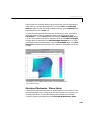
1
Partial Differential Equation Toolbox For Use with MATLAB ® Computer Solutions Europe AB Computation Visualization Programming User’s Guide How to Contact The MathWorks: ☎ 508-647-7000 Phone 508-647-7001 Fax The MathWorks, Inc. 24 Prime Park Way Natick, MA 01760-1500 Mail http://www.mathworks.com Web Anonymous FTP server Newsgroup FAX ✉ ftp.mathworks.com comp.soft-sys.matlab @ [email protected] [email protected] [email protected] [email protected] [email protected] [email protected] [email protected] Technical support Product enhancement suggestions Bug reports Documentation error reports Subscribing user registration Order status, license renewals, passcodes Sales, pricing, and general information Partial Differential Equation Toolbox User’s Guide COPYRIGHT 1984 - 1997 by The MathWorks, Inc. All Rights Reserved. The software described in this document is furnished under a license agreement. The software may be used or copied only under the terms of the license agreement. No part of this manual may be photocopied or reproduced in any form without prior written consent from The MathWorks, Inc. U.S. GOVERNMENT: If Licensee is acquiring the Programs on behalf of any unit or agency of the U.S. Government, the following shall apply: (a) For units of the Department of Defense: the Government shall have only the rights specified in the license under which the commercial computer software or commercial software documentation was obtained, as set forth in subparagraph (a) of the Rights in Commercial Computer Software or Commercial Software Documentation Clause at DFARS 227.7202-3, therefore the rights set forth herein shall apply; and (b) For any other unit or agency: NOTICE: Notwithstanding any other lease or license agreement that may pertain to, or accompany the delivery of, the computer software and accompanying documentation, the rights of the Government regarding its use, reproduction, and disclosure are as set forth in Clause 52.227-19 (c)(2) of the FAR. MATLAB, Simulink, Handle Graphics, and Real-Time Workshop are registered trademarks and Stateflow and Target Language Compiler are trademarks of The MathWorks, Inc. Other product or brand names are trademarks or registered trademarks of their respective holders. Printing History: August 1995 First printing February 1996 Reprint Contents Tutorial 1 Introduction . . . . . . . . . . . . . . . . . . . . . . . . . . . . . . . . . . . . . . . . . . 1-2 What Does this Toolbox Do? . . . . . . . . . . . . . . . . . . . . . . . . . . . . . 1-2 Can I Use the PDE Toolbox? . . . . . . . . . . . . . . . . . . . . . . . . . . . . 1-2 What Problems Can I Solve? . . . . . . . . . . . . . . . . . . . . . . . . . . . . . 1-3 In Which Areas Can the Toolbox Be Used? . . . . . . . . . . . . . . . . . 1-5 How Do I Define a PDE Problem? . . . . . . . . . . . . . . . . . . . . . . . . 1-5 How Can I Solve a PDE Problem? . . . . . . . . . . . . . . . . . . . . . . . . 1-6 Can I Use the Toolbox for Nonstandard Problems? . . . . . . . . . . 1-6 How Can I Visualize My Results? . . . . . . . . . . . . . . . . . . . . . . . . 1-6 Are There Any Applications Already Implemented? . . . . . . . . . . 1-7 Can I Extend the Functionality of the Toolbox? . . . . . . . . . . . . . 1-7 How Can I Solve 3-D Problems by 2-D Models? . . . . . . . . . . . . . 1-8 Getting Started . . . . . . . . . . . . . . . . . . . . . . . . . . . . . . . . . . . . . . . . 1-9 Basics of The Finite Element Method . . . . . . . . . . . . . . . . . . .1-18 Using the Graphical User Interface . . . . . . . . . . . . . . . . . . . . .1-23 The PDE Toolbox Graphical User Interface . . . . . . . . . . . . . . .1-23 The Menus . . . . . . . . . . . . . . . . . . . . . . . . . . . . . . . . . . . . . . . . . .1-24 The Toolbar . . . . . . . . . . . . . . . . . . . . . . . . . . . . . . . . . . . . . . . . .1-25 The GUI Modes . . . . . . . . . . . . . . . . . . . . . . . . . . . . . . . . . . . . . .1-26 The CSG Model and the Set Formula . . . . . . . . . . . . . . . . . . . .1-27 Creating Rounded Corners . . . . . . . . . . . . . . . . . . . . . . . . . . . . .1-28 Suggested Modeling Method . . . . . . . . . . . . . . . . . . . . . . . . . . . .1-31 Object Selection Methods . . . . . . . . . . . . . . . . . . . . . . . . . . . . . .1-35 Display Additional Information . . . . . . . . . . . . . . . . . . . . . . . . .1-35 Entering Parameter Values as M ATLAB Expressions . . . . . . .1-36 Using PDE Toolbox version 1.0 Model M-files . . . . . . . . . . . . . .1-36 i Using Command-Line Functions . . . . . . . . . . . . . . . . . . . . . . . Data Structures and Utility Functions . . . . . . . . . . . . . . . . . . . Constructive Solid Geometry Model . . . . . . . . . . . . . . . . . . . Decomposed Geometry . . . . . . . . . . . . . . . . . . . . . . . . . . . . . Boundary Conditions . . . . . . . . . . . . . . . . . . . . . . . . . . . . . . . Equation Coefficients . . . . . . . . . . . . . . . . . . . . . . . . . . . . . . Mesh . . . . . . . . . . . . . . . . . . . . . . . . . . . . . . . . . . . . . . . . . . . . Solution . . . . . . . . . . . . . . . . . . . . . . . . . . . . . . . . . . . . . . . . . Post Processing and Presentation . . . . . . . . . . . . . . . . . . . . . Hints and Suggestions for Using Command-Line Functions . . . . . . . . . . . . . . . . . . . . . . . . . . . . . . . . . . . . . . . . . . 1-37 1-37 1-38 1-39 1-39 1-39 1-39 1-40 1-40 1-40 Examples 2 Examples of Elliptic Problems . . . . . . . Poisson’s Equation on Unit Disk . . . . . . . Using the Graphical User Interface . . Using Command-Line Functions . . . . A Scattering Problem . . . . . . . . . . . . . . . . Using the Graphical User Interface . . A Minimal Surface Problem . . . . . . . . . . Using the Graphical User Interface . . Using Command-Line Functions . . . . Domain Decomposition . . . . . . . . . . . . . . ii Contents . . . . . . . . . . . . . . . . . . 2-2 . . . . . . . . . . . . . . . . . . 2-2 . . . . . . . . . . . . . . . . . . 2-2 . . . . . . . . . . . . . . . . . . 2-4 . . . . . . . . . . . . . . . . . . 2-6 . . . . . . . . . . . . . . . . . . 2-8 . . . . . . . . . . . . . . . . . 2-10 . . . . . . . . . . . . . . . . . 2-10 . . . . . . . . . . . . . . . . . 2-11 . . . . . . . . . . . . . . . . . 2-12 Examples of Parabolic Problems . . . . . . . . . . . . . . . . . . . . . . . The Heat Equation: A Heated Metal Block . . . . . . . . . . . . . . . . Using the Graphical User Interface . . . . . . . . . . . . . . . . . . . Using Command-Line Functions . . . . . . . . . . . . . . . . . . . . . Heat Distribution in Radioactive Rod . . . . . . . . . . . . . . . . . . . . Using the Graphical User Interface . . . . . . . . . . . . . . . . . . . 2-16 2-16 2-17 2-19 2-21 2-22 Examples of Hyperbolic Problems . . . . . . . . . . . . . . . . . . . . . The Wave Equation . . . . . . . . . . . . . . . . . . . . . . . . . . . . . . . . . . Using the Graphical User Interface . . . . . . . . . . . . . . . . . . . Using Command-Line Functions . . . . . . . . . . . . . . . . . . . . . 2-23 2-23 2-23 2-25 Examples of Eigenvalue Problems . . . . . . . . . . . . . . . . . . . . . Eigenvalues and Eigenfunctions for the L-Shaped Membrane. . . . . . . . . . . . . . . . . . . . . . . . . . . . . . . . . . . . . . . . . . Using the Graphical User Interface . . . . . . . . . . . . . . . . . . . Using Command-Line Functions . . . . . . . . . . . . . . . . . . . . . L-Shaped Membrane with Rounded Corner . . . . . . . . . . . . . . . Eigenvalues and Eigenmodes of a Square . . . . . . . . . . . . . . . . Using the Graphical User Interface . . . . . . . . . . . . . . . . . . . Using Command-Line Functions . . . . . . . . . . . . . . . . . . . . . 2-27 Application Modes . . . . . . . . . . . . . . . . . . . . . . . . . . . . . . . . . . . The Application Modes and the GUI . . . . . . . . . . . . . . . . . . . . . Structural Mechanics - Plane Stress . . . . . . . . . . . . . . . . . . . . . Example . . . . . . . . . . . . . . . . . . . . . . . . . . . . . . . . . . . . . . . . . Using the Graphical User Interface . . . . . . . . . . . . . . . . . . . Structural Mechanics - Plane Strain . . . . . . . . . . . . . . . . . . . . Electrostatics . . . . . . . . . . . . . . . . . . . . . . . . . . . . . . . . . . . . . . . Example . . . . . . . . . . . . . . . . . . . . . . . . . . . . . . . . . . . . . . . . . Using the Graphical User Interface . . . . . . . . . . . . . . . . . . . Magnetostatics . . . . . . . . . . . . . . . . . . . . . . . . . . . . . . . . . . . . . . Example . . . . . . . . . . . . . . . . . . . . . . . . . . . . . . . . . . . . . . . . . Using the Graphical User Interface . . . . . . . . . . . . . . . . . . . AC Power Electromagnetics . . . . . . . . . . . . . . . . . . . . . . . . . . . Example . . . . . . . . . . . . . . . . . . . . . . . . . . . . . . . . . . . . . . . . . Using the Graphical User Interface . . . . . . . . . . . . . . . . . . . Conductive Media DC . . . . . . . . . . . . . . . . . . . . . . . . . . . . . . . . Example . . . . . . . . . . . . . . . . . . . . . . . . . . . . . . . . . . . . . . . . . Using the Graphical User Interface . . . . . . . . . . . . . . . . . . . Heat Transfer . . . . . . . . . . . . . . . . . . . . . . . . . . . . . . . . . . . . . . . Example . . . . . . . . . . . . . . . . . . . . . . . . . . . . . . . . . . . . . . . . . Using the Graphical User Interface . . . . . . . . . . . . . . . . . . . Diffusion . . . . . . . . . . . . . . . . . . . . . . . . . . . . . . . . . . . . . . . . . . . 2-35 2-35 2-36 2-39 2-39 2-41 2-43 2-44 2-44 2-46 2-47 2-48 2-51 2-52 2-53 2-55 2-55 2-56 2-57 2-58 2-59 2-61 2-27 2-27 2-28 2-31 2-32 2-33 2-33 iii The Graphical User Interface 3 PDE Toolbox Menus . . . . . . . . . . . . . . . . . . . . . . . . . . . . . . . . . . . 3-3 File Menu . . . . . . . . . . . . . . . . . . . . . . . . . . . . . . . . . . . . . . . . . . . 3-3 New . . . . . . . . . . . . . . . . . . . . . . . . . . . . . . . . . . . . . . . . . . . . . . 3-3 Open . . . . . . . . . . . . . . . . . . . . . . . . . . . . . . . . . . . . . . . . . . . . . 3-4 Save As . . . . . . . . . . . . . . . . . . . . . . . . . . . . . . . . . . . . . . . . . . . 3-5 Print . . . . . . . . . . . . . . . . . . . . . . . . . . . . . . . . . . . . . . . . . . . . . 3-6 Edit Menu . . . . . . . . . . . . . . . . . . . . . . . . . . . . . . . . . . . . . . . . . . . 3-7 Paste . . . . . . . . . . . . . . . . . . . . . . . . . . . . . . . . . . . . . . . . . . . . . 3-8 Options Menu . . . . . . . . . . . . . . . . . . . . . . . . . . . . . . . . . . . . . . . . 3-9 Grid Spacing . . . . . . . . . . . . . . . . . . . . . . . . . . . . . . . . . . . . . 3-10 Axes Limits . . . . . . . . . . . . . . . . . . . . . . . . . . . . . . . . . . . . . . 3-11 Application . . . . . . . . . . . . . . . . . . . . . . . . . . . . . . . . . . . . . . . 3-11 Draw Menu . . . . . . . . . . . . . . . . . . . . . . . . . . . . . . . . . . . . . . . . . 3-13 Rotate . . . . . . . . . . . . . . . . . . . . . . . . . . . . . . . . . . . . . . . . . . . . . 3-14 Boundary Menu . . . . . . . . . . . . . . . . . . . . . . . . . . . . . . . . . . . . . 3-15 Specify Boundary Conditions . . . . . . . . . . . . . . . . . . . . . . . . . 3-16 PDE Menu . . . . . . . . . . . . . . . . . . . . . . . . . . . . . . . . . . . . . . . . . 3-18 PDE Specification . . . . . . . . . . . . . . . . . . . . . . . . . . . . . . . . . . 3-19 Mesh Menu . . . . . . . . . . . . . . . . . . . . . . . . . . . . . . . . . . . . . . . . . 3-22 Parameters . . . . . . . . . . . . . . . . . . . . . . . . . . . . . . . . . . . . . . . 3-23 Solve Menu . . . . . . . . . . . . . . . . . . . . . . . . . . . . . . . . . . . . . . . . . 3-25 Parameters . . . . . . . . . . . . . . . . . . . . . . . . . . . . . . . . . . . . . . . 3-25 Plot Menu . . . . . . . . . . . . . . . . . . . . . . . . . . . . . . . . . . . . . . . . . . 3-30 Parameters . . . . . . . . . . . . . . . . . . . . . . . . . . . . . . . . . . . . . . . 3-30 Additional Plot Control Options . . . . . . . . . . . . . . . . . . . . . . 3-34 Window Menu . . . . . . . . . . . . . . . . . . . . . . . . . . . . . . . . . . . . . . 3-37 Help Menu . . . . . . . . . . . . . . . . . . . . . . . . . . . . . . . . . . . . . . . . . 3-37 The Toolbar . . . . . . . . . . . . . . . . . . . . . . . . . . . . . . . . . . . . . . . . . 3-38 iv Contents The Finite Element Method 4 The Elliptic Equation . . . . . . . . . . . . . . . . . . . . . . . . . . . . . . . . . . 4-3 The Elliptic System . . . . . . . . . . . . . . . . . . . . . . . . . . . . . . . . . . 4-10 The Parabolic Equation . . . . . . . . . . . . . . . . . . . . . . . . . . . . . . 4-13 The Hyperbolic Equation. . . . . . . . . . . . . . . . . . . . . . . . . . . . . . 4-16 The Eigenvalue Equation . . . . . . . . . . . . . . . . . . . . . . . . . . . . . 4-17 Nonlinear Equations . . . . . . . . . . . . . . . . . . . . . . . . . . . . . . . . . 4-21 Adaptive Mesh Refinement . . . . . . . . . . . . . . . . . . . . . . . . . . . The Error Indicator Function . . . . . . . . . . . . . . . . . . . . . . . . . . The Mesh Refiner . . . . . . . . . . . . . . . . . . . . . . . . . . . . . . . . . . . . The Termination Criteria . . . . . . . . . . . . . . . . . . . . . . . . . . . . . 4-26 4-26 4-27 4-28 Fast Solution of Poisson’s Equation . . . . . . . . . . . . . . . . . . . . 4-29 v Reference 5 Commands Grouped by Function . . . . . . . . . . . . . . . . . . . . . . . 5-3 PDE Algorithms . . . . . . . . . . . . . . . . . . . . . . . . . . . . . . . . . . . . . . 5-3 User Interface Algorithms . . . . . . . . . . . . . . . . . . . . . . . . . . . . . . 5-3 Geometry Algorithms . . . . . . . . . . . . . . . . . . . . . . . . . . . . . . . . . . 5-4 Plot Functions . . . . . . . . . . . . . . . . . . . . . . . . . . . . . . . . . . . . . . . 5-4 Utility Algorithms . . . . . . . . . . . . . . . . . . . . . . . . . . . . . . . . . . . . 5-5 User Defined Algorithms . . . . . . . . . . . . . . . . . . . . . . . . . . . . . . . 5-7 Demonstration Programs . . . . . . . . . . . . . . . . . . . . . . . . . . . . . . 5-7 PDE Coefficients for Scalar Case . . . . . . . . . . . . . . . . . . . . . 5-20 PDE Coefficients for System Case . . . . . . . . . . . . . . . . . . . . 5-21 Boundary Condition Dialog Box . . . . . . . . . . . . . . . . . . . . . . 5-80 Model M-file . . . . . . . . . . . . . . . . . . . . . . . . . . . . . . . . . . . . . . 5-81 Index vi Contents 1 Tutorial Introduction . . . . . . . . . . . . . . . . . . . . . . . . . . . . . . . . . . . . . . . . 1-2 What Does this Toolbox Do? . . . . . . . . . . . . . . . . . . . . . . . . . . . . . 1-2 Can I Use the PDE Toolbox? . . . . . . . . . . . . . . . . . . . . . . . . . . . . . 1-2 What Problems Can I Solve? . . . . . . . . . . . . . . . . . . . . . . . . . . . . 1-3 In Which Areas Can the Toolbox Be Used? . . . . . . . . . . . . . . . . . 1-5 How Do I Define a PDE Problem? . . . . . . . . . . . . . . . . . . . . . . . . 1-5 How Can I Solve a PDE Problem? . . . . . . . . . . . . . . . . . . . . . . . . 1-6 Can I Use the Toolbox for Nonstandard Problems? . . . . . . . . . . 1-6 How Can I Visualize My Results? . . . . . . . . . . . . . . . . . . . . . . . . 1-6 Are There Any Applications Already Implemented? . . . . . . . . . 1-7 Can I Extend the Functionality of the Toolbox? . . . . . . . . . . . . . 1-7 How Can I Solve 3-D Problems by 2-D Models? . . . . . . . . . . . . . 1-8 Getting Started . . . . . . . . . . . . . . . . . . . . . . . . . . . . . . . . . . . . . 1-9 Basics of The Finite Element Method . . . . . . . . . . . . . . . . . 1-18 Using the Graphical User Interface . . . . . . . . . . . . . . . . . . 1-23 The PDE Toolbox Graphical User Interface . . . . . . . . . . . . . . . 1-23 The Menus . . . . . . . . . . . . . . . . . . . . . . . . . . . . . . . . . . . . . . . . . . 1-24 The Toolbar . . . . . . . . . . . . . . . . . . . . . . . . . . . . . . . . . . . . . . . . . 1-25 The GUI Modes . . . . . . . . . . . . . . . . . . . . . . . . . . . . . . . . . . . . . . 1-26 The CSG Model and the Set Formula . . . . . . . . . . . . . . . . . . . . 1-27 Creating Rounded Corners . . . . . . . . . . . . . . . . . . . . . . . . . . . . . 1-28 Suggested Modeling Method . . . . . . . . . . . . . . . . . . . . . . . . . . . 1-31 Object Selection Methods . . . . . . . . . . . . . . . . . . . . . . . . . . . . . . 1-35 Display Additional Information . . . . . . . . . . . . . . . . . . . . . . . . . 1-35 Entering Parameter Values as MATLAB Expressions . . . . . . . 1-36 Using PDE Toolbox version 1.0 Model M-files . . . . . . . . . . . . . 1-36 Using Command-Line Functions . . . . . . . . . . . . . . . . . . . . . 1-37 Data Structures and Utility Functions . . . . . . . . . . . . . . . 1-37 Hints and Suggestions for Using Command-Line Function . . . 1-40 1 Tutorial Introduction This section attempts to answer some of the questions you might formulate when you turn the first page: What does this toolbox do? Can I use it? What problems can I solve?, etc. What Does this Toolbox Do? The Partial Differential Equation (PDE) Toolbox provides a powerful and flexible environment for the study and solution of partial differential equations in two space dimensions and time. The equations are discretized by the Finite Element Method (FEM). The objectives of the PDE Toolbox are to provide you with tools that: • Define a PDE problem, i.e., define 2-D regions, boundary conditions, and PDE coefficients. • Numerically solve the PDE problem, i.e., generate unstructured meshes, discretize the equations, and produce an approximation to the solution. • Visualize the results. Can I Use the PDE Toolbox? The PDE Toolbox is designed for both beginners and advanced users. The minimal requirement is that you can formulate a PDE problem on paper (draw the domain, write the boundary conditions, and the PDE). Start MATLAB. At the MATLAB command line type: pdetool This invokes the graphical user interface (GUI), which is a self-contained graphical environment for PDE solving. For common applications you can use the specific physical terms rather than abstract coefficients. Using pdetool requires no knowledge of the mathematics behind the PDE, the numerical schemes, or M ATLAB. In “Getting Started” on page 1-9 we guide you through an example step by step. Advanced applications are also possible by downloading the domain geometry, boundary conditions, and mesh description to the M ATLAB workspace. From the command line (or M-files) you can call functions from the toolbox to do the hard work, e.g., generate meshes, discretize your problem, perform interpolation, plot data on unstructured grids, etc., while you retain full control over the global numerical algorithm. 1-2 Introduction What Problems Can I Solve? The basic equation of the PDE Toolbox is the PDE – ∇ ⋅ ( c ∇u ) + au = f in Ω, which we shall refer to as the elliptic equation, regardless of whether its coefficients and boundary conditions make the PDE problem elliptic in the mathematical sense. Analogously, we shall use the terms parabolic equation and hyperbolic equation for equations with spatial operators like the one above, and first and second order time derivatives, respectively. Ω is a bounded domain in the plane. c, a, f, and the unknown u are scalar, complex valued functions defined on Ω. c can be a 2-by-2 matrix function on Ω. The toolbox can also handle the parabolic PDE ∂u d----- – ∇ ⋅ ( c ∇u ) + au = f , ∂t the hyperbolic PDE 2 ∂ u d -------- – ∇ ⋅ ( c ∇u ) + au = f, 2 ∂t and the eigenvalue problem – ∇ ⋅ ( c ∇u ) + au = λdu where d is a complex valued function on Ω, and λ is an unknown eigenvalue. For the parabolic and hyperbolic PDE the coefficients c, a, f, and d can depend on time. A nonlinear solver is available for the nonlinear elliptic PDE – ∇ ⋅ ( c ( u ) ∇u ) + a ( u )u = f ( u ), where c, a, and f are functions of the unknown solution u. All solvers can handle the system case – ∇ ⋅ ( c 11 ∇u 1 ) – ∇ ⋅ ( c 12 ∇u 2 ) + a 11 u 1 + a 12 u 2 = f 1 – ∇ ⋅ ( c 21 ∇u 1 ) – ∇ ⋅ ( c 22 ∇u 2 ) + a 21 u 1 + a 22 u 2 = f 2 . You can work with systems of arbitrary dimension from the command line. For the elliptic problem, an adaptive mesh refinement algorithm is implemented. It can also be used in conjunction with the nonlinear solver. In addition, a fast solver for Poisson’s equation on a rectangular grid is available. 1-3 1 Tutorial The following boundary conditions are defined for scalar u: • Dirichlet: hu = r on the boundary ∂Ω . • Generalized Neumann: n ⋅ ( c ∇u ) + qu = g on ∂Ω . n is the outward unit normal. g, q, h, and r are complex valued functions defined on ∂Ω . (The eigenvalue problem is a homogeneous problem, i.e., g = 0, r = 0.) In the nonlinear case, the coefficients, g, q, h, and r can depend on u, and for the hyperbolic and parabolic PDE, the coefficients can depend on time. For the two-dimensional system case, Dirichlet boundary condition is h 11 u 1 + h 12 u 2 = r 1 h 21 u 1 + h 22 u 2 = r 2 , the generalized Neumann boundary condition is n ⋅ ( c 11 ∇u 1 ) + n ⋅ ( c 12 ∇u 2 ) + q 11 u 1 + q 12 u 2 = g 1 n ⋅ ( c 21 ∇u 1 ) + n ⋅ ( c 22 ∇u 2 ) + q 21 u 1 + q 22 u 2 = g 2 , and the mixed boundary condition is h 11 u 1 + h 12 u 2 = r 1 n ⋅ ( c 11 ∇u 1 ) + n ⋅ ( c 12 ∇u 2 ) + q 11 u 1 + q 12 u 2 = g 1 + h 11 µ n ⋅ ( c 21 ∇u 1 ) + n ⋅ ( c 22 ∇u 2 ) + q 21 u 1 + q 22 u 2 = g 2 + h 12 µ , where µ is computed such that the Dirichlet boundary condition is satisfied. Dirichlet boundary conditions are also called essential boundary conditions, and Neumann boundary conditions are also called natural boundary conditions. See Chapter 4, "The Finite Element Method" for the general system case. 1-4 Introduction In Which Areas Can the Toolbox Be Used? The PDEs implemented in the toolbox are used as a mathematical model for a wide variety of phenomena in all branches of engineering and science. The following is by no means a complete list of examples: The elliptic and parabolic equations are used for modeling • steady and unsteady heat transfer in solids • flows in porous media and diffusion problems • electrostatics of dielectric and conductive media • potential flow The hyperbolic equation is used for • transient and harmonic wave propagation in acoustics and electromagnetics • transverse motions of membranes The eigenvalue problems are used for, e.g., • determining natural vibration states in membranes and structural mechanics problems Last, but not least, the toolbox can be used for educational purposes as a complement to understanding the theory of the Finite Element Method. How Do I Define a PDE Problem? The simplest way to define a PDE problem is using the graphical user interface (GUI), implemented in pdetool. There are three modes that correspond to different stages of defining a PDE problem: • Draw mode, you create Ω, the geometry, using the constructive solid geometry (CSG) model paradigm. A set of solid objects (rectangle, circle, ellipse, and polygon) is provided. You can combine these objects using set formulas. • In Boundary mode, you specify the boundary conditions. You can have different types of boundary conditions on different boundary segments. • In PDE mode, you interactively specify the type of PDE and the coefficients c, a, f, and d. You can specify the coefficients for each subdomain independently. This may ease the specification of, e.g., various material properties in a PDE model. 1-5 1 Tutorial How Can I Solve a PDE Problem? Most problems can be solved from the graphical user interface. There are two major modes that help you solve a problem: • In Mesh mode, you generate and plot meshes. You can control the parameters of the automated mesh generator. • In Solve mode, you can invoke and control the nonlinear and adaptive solvers for elliptic problems. For parabolic and hyperbolic problems, you can specify the initial values, and the times for which the output should be generated. For the eigenvalue solver, you can specify the interval in which to search for eigenvalues. After solving a problem, you can return to the Mesh mode to further refine your mesh and then solve again. You can also employ the adaptive mesh refiner and solver. This option tries to find a mesh that fits the solution. Can I Use the Toolbox for Nonstandard Problems? For advanced, nonstandard applications you can transfer the description of domains, boundary conditions etc. to your MATLAB workspace. From there you use the functions of the PDE Toolbox for managing data on unstructured meshes. You have full access to the mesh generators, FEM discretizations of the PDE and boundary conditions, interpolation functions, etc. You can design your own solvers or use FEM to solve subproblems of more complex algorithms. See also the section “Using Command-Line Functions.” How Can I Visualize My Results? From the graphical user interface you can use Plot mode, where you have a wide range of visualization possibilities. You can visualize both inside the pdetool GUI and in separate figures. You can plot three different solution properties at the same time, using color, height, and vector field plots. Surface, mesh, contour, and arrow (quiver) plots are available. For surface plots, you can choose between interpolated and flat rendering schemes. The mesh may be hidden or exposed in all plot types. For parabolic and hyperbolic equations, you can even produce an animated movie of the solution’s time-dependence. All visualization functions are also accessible from the command line. 1-6 Introduction Are There Any Applications Already Implemented? The PDE Toolbox is easy to use in the most common areas due to the application interfaces. Eight application interfaces are available, in addition to the generic scalar and system (vector valued u) cases: • Structural Mechanics - Plane Stress • Structural Mechanics - Plane Strain • Electrostatics • Magnetostatics • AC Power Electromagnetics • Conductive Media DC • Heat Transfer • Diffusion These interfaces have dialog boxes where the PDE coefficients, boundary conditions, and solution are explained in terms of physical entities. The application interfaces enable you to enter specific parameters, such as Young’s modulus in the structural mechanics problems. Also, visualization of the relevant physical variables is provided. Several nontrivial examples are included in this manual. Many examples are solved both by using the GUI and in command-line mode. The toolbox contains a number of demonstration M-files. They illustrate some ways in which you can write your own applications. Can I Extend the Functionality of the Toolbox? The PDE Toolbox is written using M ATLAB’s open system philosophy. There are no black-box functions, although some functions may not be easy to understand at first glance. The data structures and formats are documented. You can examine the existing functions and create your own as needed. 1-7 1 Tutorial How Can I Solve 3-D Problems by 2-D Models? The PDE Toolbox solves problems in two space dimensions and time, whereas reality has three space dimensions. The reduction to 2-D is possible when variations in the third space dimension (taken to be z) can be accounted for in the 2-D equation. In some cases, like the plane stress analysis, the material parameters must be modified in the process of dimensionality reduction. When the problem is such that variation with z is negligible, all z-derivatives drop out and the 2-D equation has exactly the same units and coefficients as in 3-D. Slab geometries are treated by integration through the thickness. The result is a 2-D equation for the z-averaged solution with the thickness, say D(x,y), multiplied onto all the PDE coefficients, c, a, d, and f, etc. For instance, if you want to compute the stresses in a sheet welded together from plates of different thickness, multiply Young’s modulus E, volume forces, and specified surface tractions by D(x,y). Similar definitions of the equation coefficients are called for in other slab geometry examples and application modes. 1-8 Getting Started Getting Started To get you started, let’s use the graphical user interface (GUI) pdetool, which is a part of the PDE Toolbox, to solve a PDE step by step. The problem that we would like to solve is Poisson’s equation, – ∆u = f . The 2-D geometry on which we would like to solve the PDE is quite complex. The boundary conditions are of Dirichlet and Neumann types. First, invoke MATLAB. To start the GUI, type the command pdetool at the MATLAB prompt. It can take a minute or two for the GUI to start. The GUI looks similar to the figure below, with exception of the grid. Turn on the grid by selecting Grid from the Options menu. Also, enable the “snap-to-grid” feature by selecting Snap from the Options menu. The “snap-to-grid” feature simplifies aligning the solid objects. The first step is to draw the geometry on which you want to solve the PDE. The GUI provides four basic types of solid objects: polygons, rectangles, circles, and ellipses. The objects are used to create a Constructive Solid Geometry model (CSG model). Each solid object is assigned a unique label, and by the use of set algebra, the resulting geometry can be made up of a combination of unions, intersections, and set differences. By default, the resulting CSG model is the union of all solid objects. 1-9 1 Tutorial To select a solid object, either click on the button with an icon depicting the solid object that you want to use, or select the object by using the Draw pull-down menu. In this case, rectangle/square objects are selected. To draw a rectangle or a square starting at a corner, press the rectangle button without a + sign in the middle. The button with the + sign is used when you want to draw starting at the center. Then, put the cursor at the desired corner, and click-and-drag using the left mouse button to create a rectangle with the desired side lengths. (Use the right mouse button to create a square.) Notice how the “snap-to-grid” feature forces the rectangle to line up with the grid. When you release the mouse, the CSG model is updated and redrawn. At this stage, all you have is a rectangle. It is assigned the label R1. If you want to move or resize the rectangle, you can easily do so. Click-and-drag an object to move it, and double-click on an object to open a dialog box, where you can enter exact location coordinates. From the dialog box, you can also alter the label. If you are not satisfied and want to restart, you can delete the rectangle by pressing the Delete key or by selecting Clear from the Edit menu. Next, draw a circle by clicking on the button with the ellipse icon with the + sign, and then click-and-drag in a similar way, using the right mouse button, starting at the circle center. 1-10 Getting Started The resulting CSG model is the union of the rectangle R1 and the circle C1, described by set algebra as R1+C1. The area where the two objects overlap is clearly visible as it is drawn using a darker shade of gray. The object that you just drew — the circle — has a black border, indicating that it is selected. A selected object can be moved, resized, copied, and deleted. You can select more than one object by Shift-clicking on the objects that you want to select. Also, a Select All option is available from the Edit menu. Finally, add two more objects, a rectangle R2 and a circle C2. The desired CSG model is formed by subtracting the circle C2 from the union of the other three objects. You do this by editing the set formula that by default is the union of all objects: C1+R1+R2+C2. You can type any other valid set formula into Set formula edit field. Click in the edit field and use the keyboard to change the set formula to: (R1+C1+R2)-C2 1-11 1 Tutorial If you want, you can save this CSG model as an M-file. Use the Save As. . . option from the File menu, and enter a filename of your choice. It’s good practice to continue to save your model at regular intervals using Save. All the additional steps in the process of modeling and solving your PDE are then saved to the same M-file. This concludes the drawing part. You can now define the boundary conditions for the outer boundaries. Enter the Boundary mode by pressing the ∂Ω icon or by selecting Boundary Mode from the Boundary menu. You can now remove subdomain borders and define the boundary conditions. The gray edge segments are subdomain borders induced by the intersections of the original solid objects. Borders that do not represent borders between, e.g., areas with differing material properties, can be removed. From the Boundary menu, select the Remove All Subdomain Borders option. All borders are then removed from the decomposed geometry. The boundaries are indicated by colored lines with arrows. The color reflects the type of boundary condition, and the arrow points towards the end of the boundary segment. The direction information is provided for the case when the boundary condition is parameterized along the boundary. The boundary condition can also be a function of x and y, or simply a constant. By default, the boundary condition is of Dirichlet type: u = 0 on the boundary. Dirichlet boundary conditions are indicated by red color. The boundary conditions can also be of a generalized Neumann (blue) or mixed (green) type. For scalar u, however, all boundary conditions are either of Dirichlet or the generalized Neumann type. You select the boundary conditions that you want to change by clicking to select one boundary segment, by Shift-clicking to select multiple segments, or by using the Edit menu option Select All to select all boundary segments. The selected boundary segments are indicated by black color. 1-12 Getting Started For this problem, change the boundary condition for all the circle arcs. Select them by using the mouse and Shift-click on those boundary segments. Double-clicking anywhere on the selected boundary segments opens the Boundary Condition dialog box. Here, you select the type of boundary condition, and enter the boundary condition as a MATLAB expression. Change the boundary condition along the selected boundaries to a Neumann condition, ∂n ⁄ ∂u = – 5 . This means that the solution has a slope of –5 in the normal direction for these boundary segments. In the Boundary Condition dialog box, select the Neumann condition type, and enter –5 in the edit box for the boundary condition parameter g. To define a pure Neumann condition, leave the q parameter at its default value, 0. When you press the OK button, notice how the selected boundary segments change to blue to indicate Neumann boundary condition. 1-13 1 Tutorial Next, specify the PDE itself through a dialog box that is accessed by pressing the button with the PDE icon or by selecting PDE Specification. . . from the PDE pull-down menu. In the PDE mode, you can also access the PDE Specification dialog box by double-clicking on a subdomain. That way, different subdomains can have different PDE coefficient values. This problem, however, consists of only one subdomain. In the dialog box, you can select the type of PDE (elliptic, parabolic, hyperbolic, or eigenmodes) and define the applicable coefficients depending on the PDE type. This problem consists of an elliptic PDE defined by the equation – ∇ ⋅ ( c∇u ) + au = f, with c = 1.0, a = 0.0, and f = 10.0. 1-14 Getting Started Finally, create the triangular mesh that the PDE Toolbox uses in the Finite Element Method (FEM) to solve the PDE. The triangular mesh is created and displayed when pressing the button with the icon or by selecting the Mesh menu option Initialize Mesh. If you want a more accurate solution, the mesh can be successively refined by pressing the button with the four triangle icon (the Refine button) or by selecting the Refine Mesh option from the Mesh menu. Using the Jiggle Mesh option, the mesh can be jiggled to improve the triangle quality. Parameters for controlling the jiggling of the mesh, the refinement method, and other mesh generation parameters can be found in a dialog box that is opened by selecting Parameters from the Mesh menu. You can undo any change to the mesh by selecting the Mesh menu option Undo Mesh Change. Initialize the mesh, then refine it once and finally jiggle it once. We are now ready to solve the problem. Press the = button or select Solve PDE from the Solve menu to solve the PDE. The solution is then plotted. By default, the plot uses interpolated coloring and a linear color map. A colorbar is also provided to map the different shades to the numerical values of the solution. If you want, the solution can be exported as a vector to the MATLAB main workspace. 1-15 1 Tutorial There are many more plot modes available to help you visualize the solution. Press the button with the 3-D solution icon or select Parameters. . . from the Plot menu to access the dialog box for selection of the different plot options. Several plot styles are available, and the solution can be plotted in the GUI or in a separate figure as a 3-D plot. Now, select a plot where the color and the height both represent u. Choose interpolated shading and use the continuous (interpolated) height option. The default colormap is the cool colormap; a pop-up menu lets you select from a number of different colormaps. Finally, press the Plot button to plot the solution; press the Done button to save the plot setup as the current default. The solution is plotted as a 3-D plot in a separate figure window. 1-16 Getting Started The following solution plot is the result. You can use the mouse to rotate the plot in 3-D. By clicking-and-dragging the axes, the angle from which the solution is viewed can be changed. This concludes the first example of solving a PDE by using the pdetool GUI. Many more examples in Chapter 2, "Examples" focus on solving particular problems involving different kinds of PDEs, geometries and boundary conditions and covering a range of different applications. 1-17 1 Tutorial Basics of The Finite Element Method The solutions of simple PDEs on complicated geometries can rarely be expressed in terms of elementary functions. You are confronted with two problems: First you need to describe a complicated geometry and generate a mesh on it. Then you need to discretize your PDE on the mesh and build an equation for the discrete approximation of the solution. The pdetool graphical user interface provides you with easy-to-use graphical tools to describe complicated domains and generate triangular meshes. It also discretizes PDEs, finds discrete solutions and plots results. You can access the mesh structures and the discretization functions directly from the command line (or M-file) and incorporate them into specialized applications. Below is an overview of the Finite Element Method (FEM). The purpose of this presentation is to get you acquainted with the elementary FEM notions. Here you find the precise equations that are solved and the nature of the discrete solution. Different extensions of the basic equation implemented in the PDE Toolbox are presented. A more detailed description can be found in Chapter 4, "The Finite Element Method". You start by approximating the computational domain Ω with a union of simple geometric objects, in this case triangles. The triangles form a mesh and each vertex is called a node. You are in the situation of an architect designing a dome. He has to strike a balance between the ideal rounded forms of the original sketch and the limitations of his simple building-blocks, triangles or quadrilaterals. If the result does not look close enough to a perfect dome, the architect can always improve his work using smaller blocks. Next you say that your solution should be simple on each triangle. Polynomials are a good choice: they are easy to evaluate and have good approximation properties on small domains. You can ask that the solutions in neighboring triangles connect to each other continuously across the edges. You can still decide how complicated the polynomials can be. Just like an architect, you want them as simple as possible. Constants are the simplest choice but you cannot match values on neighboring triangles. Linear functions come next. 1-18 Basics of The Finite Element Method This is like using flat tiles to build a waterproof dome, which is perfectly possible. 0.8 0.8 0.6 0.6 0.4 0.4 0.2 0.2 0 0 −1 −1 −0.5 −0.5 0 0 −1 −1 0.5 −0.5 0.5 −0.5 0 0 1 0.5 1 1 0.5 1 A triangular mesh (left) and a continuous piecewise linear function on that mesh Now you use the basic elliptic equation: – ∇ ⋅ ( c ∇u ) + au = f in Ω. If uh is the piecewise linear approximation to u, it is not clear what the second derivative term means. Inside each triangle, ∇u h is a constant (because uh is flat) and thus the second-order term vanishes. At the edges of the triangles, c ∇u h is in general discontinuous and a further derivative makes no sense. What you are looking for is the best approximation of u in the class of continuous piecewise polynomials. Therefore you test the equation for uh against all possible functions v of that class. Testing means formally to multiply the residual against any function and then integrate, i.e., determine uh such that ∫Ω ( –∇ ⋅ ( c ∇uh ) + au h – f )v dx = 0 for all possible v. The functions v are usually called test functions. Partial integration (Green’s formula) yields that uh should satisfy ∫Ω ( c ∇uh ) ∇v + auh vdx – ∫∂Ω n ⋅ ( c ∇u h )vds = ∫Ω fv dx ∀v , 1-19 1 Tutorial where ∂Ω is the boundary of Ω and n is the outward pointing normal on ∂Ω . Note that the integrals of this formulation are well-defined even if uh and v are piecewise linear functions. Boundary conditions are included in the following way. If uh is known at some boundary points (Dirichlet boundary conditions), we restrict the test functions to v = 0 at those points, and require uh to attain the desired value at that point. At all the other points we ask for Neumann boundary conditions, i.e., ( c∇u h ) ⋅ n + qu h = g . The FEM formulation reads: Find uh such that ∫Ω ( c ∇u h ) ∇v + au h vdx + ∫∂Ω quh vds = ∫Ω fv dx + ∫∂Ω gv ds 1 1 ∀v, where ∂Ω 1 is the part of the boundary with Neumann conditions. The test functions v must be zero on ∂Ω – ∂Ω 1 . Any continuous piecewise linear uh is represented as a combination uh( x) = ∑i = 1 Ui φi ( x ) , where φi are some special piecewise linear basis N functions and Ui are scalar coefficients. Choose φi like a tent, such that it has the “height” 1 at the node i and the height 0 at all other nodes. For any fixed v, the FEM formulation yields an algebraic equation in the unknowns Ui. You want to determine N unknowns, so you need N different instances of v. What better candidates than v = φj, j = 1, 2, . . . , N? You find a linear system KU = F where the matrix K and the right-hand side F contain integrals in terms of the test functions φi, φj and the coefficients defining the problem: c, a, f, q, and g. The solution vector U contains the expansion coefficients of uh, which are also the values of uh at each node xi since uh(xi) = Ui. If the exact solution u is smooth, then FEM computes uh with an error of the same size as that of the linear interpolation. It is possible to estimate the error on each triangle using only uh and the PDE coefficients (but not the exact solution u, which in general is unknown). The PDE Toolbox provides functions that assemble K and F. This is done automatically in the graphical user interface, but you also have direct access to the FEM matrices from the command-line function assempde. To summarize, the FEM approach is to approximate the PDE solution u by a piecewise linear function u h ⋅ u h is expanded in a basis of test-functions φi, and the residual is tested against all the basis functions. This procedure yields a linear system KU = F. The components of U are the values of uh at the nodes. 1-20 Basics of The Finite Element Method For x inside a triangle, uh(x) is found by linear interpolation from the nodal values. FEM techniques are also used to solve more general problems. Below are some generalizations that you can access both through the graphical user interface and with command-line functions. • Time-dependent problems are easy to implement in the FEM context. The solution u(x,t) of the equation ∂u d ----- – ∇ ⋅ ( c ∇u ) + au = f ∂t can be approximated by u h ( x, t ) = ∑i = 1 U i ( t )φ i( x ) . This yields a system of N d ordinary differential equations (ODE) M U + KU = F which you integrate dt using ODE solvers. Two time derivatives yield a second order ODE d 2 U + KU = F , etc. The toolbox supports problems with one or two time 2 dt derivatives (the functions parabolic and hyperbolic). M • Eigenvalue problems: Solve – ∇ ⋅ ( c∇u ) + au = λdu for the unknowns u and λ (λ is a complex number). Using the FEM discretization, you solve the algebraic eigenvalue problem KU = λhMU to find uh and λh as approximations to u and λ. A robust eigenvalue solver is implemented in pdeeig. • If the coefficients c, a, f, q, or g are functions of u, the PDE is called nonlinear and FEM yields a nonlinear system K(U) U= F(U). You can use iterative methods for solving the nonlinear system. The toolbox provides a nonlinear solver called pdenonlin using a damped Gauss-Newton method. 1-21 1 Tutorial • Small triangles are needed only in those parts of the computational domain where the error is large. In many cases the errors are large in a small region and making all triangles small is a waste of computational effort. Making small triangles only where needed is called adapting the mesh refinement to the solution. An iterative adaptive strategy is the following: For a given mesh, form and solve the linear system KU = F. Then estimate the error and refine the triangles in which the error is large. The iteration is controlled by adaptmesh and the error is estimated by pdejmps. Although the basic equation is scalar, systems of equations are also handled by the toolbox. The interactive environment accepts u as a scalar or 2-vector function. In command-line mode, systems of arbitrary size are accepted. If c ≥ δ > 0 and a ≥ 0, under rather general assumptions on the domain Ω and the boundary conditions, the solution u exists and is unique. The FEM linear system has a unique solution which converges to u as the triangles become smaller. The matrix K and the right-hand side F make sense even when u does not exist or is not unique. It is advisable that you devise checks to problems with questionable solutions. 1-22 Using the Graphical User Interface Using the Graphical User Interface The PDE Toolbox Graphical User Interface The PDE Toolbox includes a complete graphical user interface (GUI), which covers all aspects of the PDE solution process. You start it by typing: pdetool at the MATLAB command line. It may take a while the first time you launch pdetool during a MATLAB session. The figure below shows the pdetool GUI as it looks when you have started it. At the top, the GUI has a pull-down menu bar that you use to control the modeling. It conforms to common pull-down menu standards. Menu items followed by a right arrow lead to a submenu. Menu items followed by an ellipsis lead to a dialog box. Stand-alone menu items lead to direct action. Below the menu bar, a toolbar with icon buttons provide quick and easy access to some of the most important functions. 1-23 1 Tutorial To the right of the toolbar is a pop-up menu that indicates the current application mode. You can also use it to change the application mode. The upper right part of the GUI also provides the x- and y-coordinates of the current cursor position. It is updated when you move the cursor inside the main axes area in the middle of the GUI. The edit box for the set formula contains the active set formula. In the main axes you draw the 2-D geometry, display the mesh, plot the solution, etc. At the bottom of the GUI, an information line provides information about the current activity. It can also display help information about the toolbar buttons. The Menus There are 11 different pull-down menus in the GUI. For a more detailed description of the menus and the dialog boxes, see Chapter 3, "The Graphical User Interface". • File menu. From the File menu you can Open and Save model M-files that contain a command sequence that reproduces your modeling session. You can also print the current graphics and exit the GUI. • Edit menu. From the Edit menu you can cut, clear, copy, and paste the solid objects. There is also a Select All option. • Options menu. The Options menu contains options such as toggling the axis grid, a “snap-to-grid” feature, and zoom. You can also adjust the axis limits and the grid spacing, select the application mode, and refresh the GUI. • Draw menu. From the Draw menu you can select the basic solid objects such as circles and polygons. You can then draw objects of the selected type using the mouse. From the Draw menu you can also rotate the solid objects and export the geometry to the MATLAB main workspace. • Boundary menu. From the Boundary menu you access a dialog box where you define the boundary conditions. Additionally, you can label edges and subdomains, remove borders between subdomains, and export the decomposed geometry and the boundary conditions to the workspace. • PDE menu. The PDE menu provides a dialog box for specifying the PDE, and there are menu options for labeling subdomains and exporting PDE coefficients to the workspace. 1-24 Using the Graphical User Interface • Mesh menu. From the Mesh menu you create and modify the triangular mesh. You can initialize, refine, and jiggle the mesh, undo previous mesh changes, label nodes and triangles, display the mesh quality, and export the mesh to the workspace. • Solve menu. From the Solve menu you solve the PDE. You can also open a dialog box where you can adjust the solve parameters, and you can export the solution to the workspace. • Plot menu. From the Plot menu you can plot a solution property. A dialog box lets you select which property to plot, which plot style to use and several other plot parameters. If you have recorded a movie (animation) of the solution, you can export it to the workspace. • Window menu. The Window menu lets you select any currently open M ATLAB figure window. The selected window is brought to the front. • Help menu. The Help menu provides a brief help window. The Toolbar The toolbar underneath the main menu at the top of the GUI contains icon buttons that provide quick and easy access to some of the most important functions. The five left-most buttons are Draw mode buttons and they represent, from left to right: • Draw a rectangle/square starting at a corner. • Draw a rectangle/square starting at the center. • Draw an ellipse/circle starting at the perimeter. • Draw an ellipse/circle starting at the center. • Draw a polygon. Click-and-drag to create polygon sides. You can close the polygon by pressing the right mouse button. Clicking at the starting vertex also closes the polygon. The Draw mode buttons can only be activated one at the time and they all work the same way: single-clicking on a button allows you to draw one solid object of the selected type. Double-clicking on a button makes it “stick,” and you can then continue to draw solid objects of the selected type until you single-click on the button to “release” it. Using the right mouse button or Control-click, the drawing is constrained to a square or a circle. 1-25 1 Tutorial The second group of six buttons includes the following buttons: • ∂Ω : Enters the Boundary mode. • PDE: Opens the PDE Specification dialog box. • Initializes the triangular mesh. • The refine button (the four triangle icon): Refines the triangular mesh. • =: Solves the PDE. • The 3-D solution plot icon: Opens the Plot Selection dialog box. The right-most button with the magnifying glass toggles the zoom function on/off. The GUI Modes The PDE solving process can be divided into several steps: 1 Define the geometry (2-D domain). 2 Define the boundary conditions. 3 Define the PDE. 4 Create the triangular mesh. 5 Solve the PDE. 6 Plot the solution and other physical properties calculated from the solution (post processing). The pdetool GUI is designed in a similar way. You work in six different modes, each corresponding to one of the steps in the PDE solving process: • In Draw mode, you can create the 2-D geometry using the constructive solid geometry (CSG) model paradigm. A set of solid objects (rectangle, circle, ellipse, and polygon) is provided. These objects can be combined using set formulas in a flexible way. • In Boundary mode, you can specify the boundary conditions. You can have different types of boundary conditions on different boundaries. In this mode, the original shapes of the solid objects constitute borders between subdomains of the model. Such borders can be eliminated in this mode. 1-26 Using the Graphical User Interface • In PDE mode, you can interactively specify the type of PDE problem, and the PDE coefficients. You can specify the coefficients for each subdomain independently. This makes it easy to specify, e.g., various material properties in a PDE model. • In Mesh mode, you can control the automated mesh generation and plot the mesh. • In Solve mode, you can invoke and control the nonlinear and adaptive solver for elliptic problems. For parabolic and hyperbolic PDE problems, you can specify the initial values, and the times for which the output should be generated. For the eigenvalue solver, you can specify the interval in which to search for eigenvalues. • In Plot mode there is wide range of visualization possibilities. You can visualize both in the pdetool GUI and in a separate figure window. You can visualize three different solution properties at the same time, using color, height, and vector field plots. There are surface, mesh, contour, and arrow (quiver) plots available. For parabolic and hyperbolic equations, you can animate the solution as it changes with time. The CSG Model and the Set Formula The PDE Toolbox uses the Constructive Solid Geometry (CSG) model paradigm for the modeling. You can draw solid objects that can overlap. There are four types of solid objects: • Circle object — represents the set of points inside and on a circle. • Polygon object — represents the set of points inside and on a polygon given by a set of line segments. • Rectangle object — represents the set of points inside and on a rectangle. • Ellipse object — represents the set of points inside and on an ellipse. The ellipse can be rotated. Each solid object is automatically given a unique name by the GUI. The default names are C1, C2, C3, etc., for circles; P1, P2, P3, etc. for polygons; R1, R2, R3, etc., for rectangles; E1, E2, E3, etc., for ellipses. Squares, although just a special case of rectangles, are named SQ1, SQ2, SQ3, etc. The name is displayed on the solid object itself. You can use any unique name, as long as it contains no blanks. In Draw mode you can alter the names and the geometries of the objects by double-clicking on them. This opens a dialog box where you can 1-27 1 Tutorial edit the name and the geometry. The following figure shows an object dialog box for a circle. You can use the name of the object to refer to the corresponding set of points in a set formula. The operators +, *, and – are used to form the set of points Ω in the plane over which the differential equation is solved. The operators +, the set union operator, and *, the set intersection operator, have the same precedence. The operator –, the set difference operator, has higher precedence. The precedence can be controlled by using parentheses. The resulting geometrical model, Ω, is the set of points for which the set formula evaluates to true. By default, it is the union of all solid objects. We often refer to the area Ω as the decomposed geometry. Creating Rounded Corners As an example of how to use the set formula, let’s model a plate with rounded corners (fillets). Start the GUI and turn on the grid and the “snap-to-grid” feature using the Options menu. Also, change the grid spacing to -1.5:0.1:1.5 for the x-axis and -1:0.1:1 for the y-axis. Select Rectangle/square from the Draw menu or press the button with the rectangle icon. Then draw a rectangle with a width of 2 and a height of 1 using the mouse, starting at (-1,0.5). To get the round corners, add circles, one in each corner. The circles should have a radius of 0.2 and centers at a distance that is 0.2 units from the left/right and lower/upper rectangle boundaries ((-0.8,-0.3), (-0.8,0.3), (0.8,-0.3), and (0.8,0.3)). To draw several circles, double-click on the button for drawing ellipses/circles (centered). Then draw the circles using the right mouse button or Control-click starting at the circle centers. Finally, at each of the rectangle corners, draw four small squares with a side of 0.1. 1-28 Using the Graphical User Interface The figure below shows the complete drawing. Now you have to edit the set formula. To get the rounded corners, subtract the small squares from the rectangle and then add the circles. As a set formula, this is expressed as R1-(SQ1+SQ2+SQ3+SQ4)+C1+C2+C3+C4 1-29 1 Tutorial Enter the set formula into the edit box at the top of the GUI. Then enter the Boundary mode by pressing the ∂Ω button or by selecting the Boundary Mode option from the Boundary menu. The CSG model is now decomposed using the set formula, and you get a rectangle with rounded corners, as shown below. Because of the intersection of the solid objects used in the initial CSG model, a number of subdomain borders remain. They are drawn using gray lines. If this is a model of, e.g., a homogeneous plate, you can remove them. Select the Remove All Subdomain Borders option from the Boundary menu. The subdomain borders are removed and the model of the plate is now complete. 1-30 Using the Graphical User Interface Suggested Modeling Method Although the PDE Toolbox offers you a great deal of flexibility in the ways that you can approach the problems and interact with the toolbox functions, there is a suggested method of choice for modeling and solving your PDE problems using the pdetool GUI. There are also a number of shortcuts that you can use in certain situations. NOTE: There are platform-dependent keyboard accelerators available for many of the most common pdetool GUI activities. Learning to use the accelerator keys may improve the efficiency of your pdetool sessions. The basic flow of actions is indicated by the way the graphical push buttons and the menus are ordered from left to right. You work your way from left to right in the process of modeling, defining, and solving your PDE problem using the pdetool GUI. • When you start, pdetool is in a Draw mode, where you can use the four basic solid objects to draw your Constructive Solid Geometry (CSG) model. You can also edit the set formula. The solid objects are selected using the five left-most push buttons (or from the Draw menu). • To the right of the Draw mode buttons you find push buttons through which you can access all the functions that you need to define and solve the PDE problem: define boundary conditions, design the triangular mesh, solve the PDE, and plot the solution. The following sequence of actions covers all the steps of a normal pdetool session: 1 Use pdetool as a drawing tool to make a drawing of the 2-D geometry on which you want to solve your PDE. Make use of the four basic solid objects and the grid and the “snap-to-grid” feature. The GUI starts in the Draw mode, and you can select the type of object that you want to use by clicking on the corresponding button or by using the Draw pull-down menu. Combine the solid objects and the set algebra to build the desired CSG model. 1-31 1 Tutorial 2 Save the geometry to a model file. The model file is an M-file, so if you want to continue working using the same geometry at your next PDE Toolbox session, simply type the name of the model file at the MATLAB prompt. The pdetool GUI then starts with the model file’s solid geometry loaded. If you save the PDE problem at a later stage of the solution process, the model file also contains commands to recreate the boundary conditions, the PDE coefficients, and the mesh. 3 Move to the next step in the PDE solving process by pressing the ∂Ω button. The outer boundaries of the decomposed geometry are displayed with the default boundary condition indicated. If the outer boundaries do not match the geometry of your problem, re-enter the Draw mode. You can then correct your CSG model by adding, removing or altering any of the solid objects, or change the set formula used to evaluate the CSG model. NOTE: The set formula can only be edited while you are in the Draw mode. If the drawing process resulted in any unwanted subdomain borders, remove them by using the Remove Subdomain Border or Remove All Subdomain Borders option from the Boundary menu. You can now define your problem’s boundary conditions by selecting the boundary to change and open a dialog box by double-clicking on the boundary or by using the Specify Boundary Conditions. . . option from the Boundary menu. 4 Initialize the triangular mesh. Press the button or use the corresponding Mesh menu option Initialize Mesh. Normally, the mesh algorithm’s default parameters generate a good mesh. If necessary, they can be accessed using the Parameters. . . menu item. 5 If you need a finer mesh, the mesh can be refined by pressing the Refine button. Pressing the button several times causes a successive refinement of the mesh. The cost of a very fine mesh is a significant increase in the number of points where the PDE is solved and, consequently, a significant increase in the time required to compute the solution. Don’t refine unless it is required to achieve the desired accuracy. For each refinement, the number of triangles increases by a factor of four. A better way to increase the 1-32 Using the Graphical User Interface accuracy of the solution to elliptic PDE problems is to use the adaptive solver, which refines the mesh in the areas where the estimated error of the solution is largest. See the entry on adaptmesh in Chapter 5, "Reference" for an example of how the adaptive solver can solve a Laplace equation with an accuracy that requires more than 10 times as many triangles when regular refinement is used. 6 Specify the PDE from the PDE Specification dialog box. You can access that dialog box using the PDE button or the PDE Specification. . . menu item from the PDE menu. NOTE: This step can be performed at any time prior to solving the PDE since it is independent of the CSG model and the boundaries. If the PDE coefficients are material dependent, they are entered in the PDE mode by double-clicking on the different subdomains. 7 Solve the PDE by pressing the = button or by selecting Solve PDE from the Solve menu. If you don’t want an automatic plot of the solution, or if you want to change the way the solution is presented, you can do that from the Plot Selection dialog box prior to solving the PDE. You open the Plot Selection dialog box by pressing the button with the 3-D solution plot icon or by selecting the Parameters. . . menu item from the Plot menu. 8 Now, from here you can choose one of several alternatives: • Export the solution and/or the mesh to MATLAB’s main workspace for further analysis. • Visualize other properties of the solution. • Change the PDE and recompute the solution. • Change the mesh and recompute the solution. If you select Initialize Mesh, the mesh is initialized; if you select Refine Mesh, the current mesh is refined. From the Mesh menu, you can also jiggle the mesh and undo previous mesh changes. • Change the boundary conditions. To return to the mode where you can select boundaries, use the ∂Ω button or the Boundary Mode option from the Boundary menu. 1-33 1 Tutorial • Change the CSG model. You can re-enter the draw mode by selecting Draw Mode from the Draw menu or by clicking on one of the Draw mode icons to add another solid object. Back in the Draw mode, you are able to add, change, or delete solid objects and also to alter the set formula. In addition to the recommended path of actions, there are a number of shortcuts, which allow you to skip over one or more steps. In general, the pdetool GUI adds the necessary steps automatically. • If you haven’t yet defined a CSG model, and leave the Draw mode with an empty model, pdetool creates an L-shaped geometry with the default boundary condition and then proceeds to the action called for, performing all the steps necessary. • If you are in the Draw mode and press the ∆ button to initialize the mesh, pdetool first decomposes the geometry using the current set formula and assigns the default boundary condition to the outer boundaries. After that, an initial mesh is created. • If you press the refine button to refine the mesh before the mesh has been initialized, pdetool first initializes the mesh (and decomposes the geometry, if you were still in the Draw mode). • If you press the = button to solve the PDE and you have not yet created a mesh, pdetool initializes a mesh before solving the PDE. • If you select a plot type and choose to plot the solution, pdetool checks to see if there is a solution to the current PDE available. If not, pdetool first solves the current PDE. The solution is then displayed using the selected plot options. • If you haven’t defined your PDE, pdetool solves the default PDE, which is Poisson’s equation: -∆ u= 10 (This corresponds to the generic elliptic PDE with c = 1, a = 0, and f = 10.) For the different application modes, different default PDE settings apply. 1-34 Using the Graphical User Interface Object Selection Methods Throughout the GUI, similar principles apply for selecting objects such as solid objects, subdomains, and boundaries. • To select a single object, click on it using the left mouse button. • To select several objects and to deselect objects, Shift-click (or click using the middle mouse button) on the desired objects. • Clicking in the intersection of several objects selects all the intersecting objects. • To open an associated dialog box, double-click on an object. If the object is not selected, it is selected before opening the dialog box. • In Draw mode and PDE mode, clicking outside of objects deselects all objects. • To select all objects, use the Select All option from the Edit menu. • When defining boundary conditions and the PDE via the menu items from the Boundary and PDE menus, and no boundaries or subdomains are selected, the entered values applies to all boundaries and subdomains by default. Display Additional Information In Mesh mode, you can use the mouse to display the node number and the triangle number at the position where you click. Press the left mouse button to display the node number on the information line. Press the middle mouse button (or use the left mouse button and the Shift key) to display the triangle number on the information line. In Plot mode, you can use the mouse to display the numerical value of the plotted property at the position where you click. Press the left mouse button to display the triangle number and the value of the plotted property on the information line. The information remains on the information line until you release the mouse button. 1-35 1 Tutorial Entering Parameter Values as MATLAB Expressions When entering parameter values, e.g., as a function of x and y, the entered string must be a M ATLAB expression to be evaluated for x and y defined on the current mesh, i.e., x and y are MATLAB row vectors. For example, the function 4 x y should be entered as 4*x.*y and not as 4*x*y, which normally is not a valid M ATLAB expression. Using PDE Toolbox version 1.0 Model M-files You can convert Model M-files created using version 1.0 of the PDE Toolbox for MATLAB 4.2 for use with PDE Toolbox version 1.0.2 and MATLAB 5. The old Model M-files cannot be used directly in PDE Toolbox 1.0.2 To convert your old Model M-files, use the conversion utility pdemdlcv. To convert a Model M-file called model42.m to a PDE Toolbox 1.0.2 compatible Model M-file called model5.m, type the following at the MATLAB command line: pdemdlcv model42 model5 1-36 Using Command-Line Functions Using Command-Line Functions Although the pdetool GUI provides a convenient working environment, there are situations where the flexibility of using the command-line functions is needed. These include: • Geometrical shapes other than straight lines, circular arcs, and elliptical arcs • Nonstandard boundary conditions • Complicated PDE or boundary condition coefficients • More than two dependent variables in the system case • Nonlocal solution constraints • Special solution data processing and presentation itemize The GUI can still be a valuable aid in some of the situations presented above, if part of the modeling is done using the GUI and then made available for command-line use through the extensive data export facilities of the GUI. Data Structures and Utility Functions The process of defining your problem and solving it is reflected in the design of the GUI. A number of data structures define different aspects of the problem, and the various processing stages produce new data structures out of old ones. See the figure on the next page. The rectangles are functions, and ellipses are data represented by matrices or M-files. Arrows indicate data necessary for the functions. As there is a definite direction in this diagram, you can cut into it by presenting the needed data sets, and then continue downward. In the sections below we give pointers to descriptions of the precise formats of the various data structures and M-files. 1-37 1 Tutorial Geometry Description matrix decsg Decomposed Geometry matrix Geometry M-file initmesh Boundary Condition matrix Boundary M-file Mesh data refinemesh Coefficient matrix Coefficient M-file assempde Solution data pdeplot Constructive Solid Geometry Model A Constructive Solid Geometry (CSG) model is specified by a Geometry Description matrix, a set formula, and a Name Space matrix. These data structures are described in the Reference chapter entry on decsg. At this level, the problem geometry is defined by overlapping solid objects. These can be created by drawing the CSG model in the GUI and then exporting the data using the Export Geometry Description, Set Formula, Labels. . . option from the Draw menu. 1-38 Using Command-Line Functions Decomposed Geometry A decomposed geometry is specified by either a Decomposed Geometry matrix, or by a Geometry M-file. Here, the geometry is described as a set of disjoint minimal regions bounded by boundary segments and border segments. A Decomposed Geometry matrix can be created from a CSG model by using the function decsg. It can also be exported from the GUI by selecting the Export Decomposed Geometry, Boundary Cond’s. . . option from the Boundary menu. A Geometry M-file equivalent to a given Decomposed Geometry matrix can be created using the wgeom function. A decomposed geometry can be visualized with the pdegplot function. The data structures of the Decomposed Geometry matrix and Geometry M-file are described in Chapter 5, "Reference" entries on decsg, and pdegeom, respectively. Boundary Conditions These are specified by either a Boundary Condition matrix, or a Boundary M-file. Boundary conditions are given as functions on boundary segments. A Boundary Condition matrix can be exported from the GUI by selecting the Export Decomposed Geometry, Boundary Cond’s. . . option from the Boundary menu. A Boundary M-file equivalent to a given Boundary Condition matrix can be created using the wbound function. The data structures of the Boundary Condition matrix and Boundary M-file are described in Chapter 5, "Reference" entries on assemb and pdebound respectively. Equation Coefficients The PDE is specified by either a Coefficient matrix or a Coefficient M-file for each of the PDE coefficients c, a, f, and d. The coefficients are functions on the subdomains. Coefficients can be exported from the GUI by selecting the Export PDE Coefficients. . . option from the PDE menu. The details on the equation coefficient data structures are given in the Chapter 5, "Reference" entry on assempde. Mesh A triangular mesh is described by the mesh data which consists of a Point matrix, an Edge matrix, and a Triangle matrix. In the mesh, minimal regions are triangulated into subdomains, and border segments and boundary segments are broken up into edges. Mesh data is created from a decomposed geometry by the function initmesh and can be altered by the functions 1-39 1 Tutorial refinemesh and jigglemesh. The Export Mesh. . . option from the Mesh menu provides another way of creating mesh data. The adaptmesh function creates mesh data as part of the solution process. The mesh may be plotted with the pdemesh function. The details on the mesh data representation are given in the Reference entry on initmesh. Solution The solution of a PDE problem is represented by the solution vector. A solution gives the value at each mesh point of each dependent variable, perhaps at several points in time, or connected with different eigenvalues. Solution vectors are produced from the mesh, the boundary conditions, and the equation coefficients by assempde, pdenonlin, adaptmesh, parabolic, hyperbolic, and pdeeig. The Export Solution. . . option from the Solve menu exports solutions to the workspace. Since the meaning of a solution vector is dependent on its corresponding mesh data, they are always used together when a solution is presented. The details on solution vectors are given in the Chapter 5, "Reference" entry on assempde. Post Processing and Presentation Given a solution/mesh pair, a variety of tools is provided for the visualization and processing of the data. pdeintrp and pdeprtni can be used to interpolate between functions defined at triangle nodes and functions defined at triangle midpoints. tri2grid interpolates a functions from a triangular mesh to a rectangular grid. pdegrad and pdecgrad compute gradients of the solution. pdeplot has a large number of options for plotting the solution. pdecont and pdesurf are convenient shorthands for pdeplot. Hints and Suggestions for Using Command-Line Functions Several examples of command-line function usage are given in the Examples chapter. Use the export facilities of the GUI as much as you can. They provide data structures with the correct syntax, and these are good starting points that you can modify to suit your needs. A good way to produce a Geometry M-file describing a geometry outside of the possibilities provided by the GUI, is to draw a similar geometry using the GUI, export the Decomposed Geometry matrix, and write a Geometry M-file with wgeom. The special segments can then be edited by hand. An example of a 1-40 Using Command-Line Functions hand-tailored Geometry M-file is cardg, also presented in the Chapter 5, "Reference" entry on pdegeom. Working with the system matrices and vectors produced by assema and assemb can sometimes be valuable. When solving the same equation for different loads or boundary conditions, it pays to assemble the stiffness matrix only once. Point loads on a particular node can be implemented by adding the load to the corresponding row in the right-hand side vector. A non-local constraint can be incorporated into the H and R matrices. An example of a hand-written Coefficient M-file is circlef that produces a point load. You can find the full example in pdedemo7 and in the Reference entry on assempde. The routines for adaptive mesh generation and solution are powerful but can lead to dense meshes and thus long computation times. Setting the Ngen parameter to one limits you to a single refinement step. This step can then be repeated to show the progress of the refinement. The Maxt parameter helps you stop before the adaptive solver generates too many triangles. An example of a hand-written triangle selection function is circlepick, used in pdedemo7. Remember that you always need a decomposed geometry with adaptmesh. Deformed meshes are easily plotted by adding offsets to the Point matrix p. Assuming two variables stored in the solution vector u: np=size(p,2); pdemesh(p+scale*[u(1:np) u(np+1:np+np)]',e,t) The time evolution of eigenmodes is obtained by, e.g., u1=u(:,mode)*cos(sqrt(l(mode))*tlist) % hyperbolic for positive eigenvalues in hyperbolic problems, or u1=u(:,mode)*exp(-l(mode)*tlist); % parabolic in parabolic problems. This makes nice animations, perhaps together with deformed mesh plots. 1-41 1 Tutorial 1-42 2 Examples Examples of Elliptic Problems . . . . . . . . . . . . . . . . . . . . . . . . 2-2 Poisson’s Equation on Unit Disk. . . . . . . . . . . . . . . . . . . . . . . . . . 2-2 A Scattering Problem . . . . . . . . . . . . . . . . . . . . . . . . . . . . . . . . . . 2-6 A Minimal Surface Problem . . . . . . . . . . . . . . . . . . . . . . . . . . . . 2-10 Domain Decomposition . . . . . . . . . . . . . . . . . . . . . . . . . . . . . . . . 2-12 Examples of Parabolic Problems . . . . . . . . . . . . . . . . . . . . . 2-16 The Heat Equation: A Heated Metal Block . . . . . . . . . . . . . . . 2-16 Heat Distribution in Radioactive Rod . . . . . . . . . . . . . . . . . . . . 2-21 Examples of Hyperbolic Problems . . . . . . . . . . . . . . . . . . . 2-23 The Wave Equation . . . . . . . . . . . . . . . . . . . . . . . . . . . . . . . . . . . 2-23 Examples of Eigenvalue Problems . . . . . . . . . . . . . . . Eigenvalues and Eigenfunctions for the L-Shaped Membrane . . . . . . . . . . . . . . . . . . . . . . . . . . . . . . . . . . L-Shaped Membrane with Rounded Corner . . . . . . . . . . . Eigenvalues and Eigenmodes of a Square . . . . . . . . . . . . . . . . . 2-27 . . . 2-27 . . . . 2-31 . . . . 2-32 Application Modes . . . . . . . . . . . . . . . . . . . . . . . . . . . . . . . . . . 2-35 The Application Modes and the GUI . . . . . . . . . . . . . . . . . . . . . 2-35 Structural Mechanics - Plane Stress . . . . . . . . . . . . . . . . . . . . . 2-36 Structural Mechanics - Plane Strain . . . . . . . . . . . . . . . . . . . . . 2-41 Electrostatics . . . . . . . . . . . . . . . . . . . . . . . . . . . . . . . . . . . . . . . . 2-43 Magnetostatics . . . . . . . . . . . . . . . . . . . . . . . . . . . . . . . . . . . . . . 2-46 AC Power Electromagnetics . . . . . . . . . . . . . . . . . . . . . . . . . . . . 2-51 Conductive Media DC . . . . . . . . . . . . . . . . . . . . . . . . . . . . . . . . . 2-55 Heat Transfer . . . . . . . . . . . . . . . . . . . . . . . . . . . . . . . . . . . . . . . 2-57 Diffusion . . . . . . . . . . . . . . . . . . . . . . . . . . . . . . . . . . . . . . . . . . . 2-61 2 Examples Examples of Elliptic Problems This section describes the solution of some elliptic PDE problems. The last problem, a minimal surface problem, is nonlinear and illustrates the use of the nonlinear solver. The problems are solved using both the graphical user interface and the command-line functions of the PDE Toolbox. Poisson’s Equation on Unit Disk As a first example of an elliptic problem, let’s use the simplest elliptic PDE of all — Poisson’s equation. The problem formulation is –∆U = 1 in Ω, U = 0 on ∂Ω where Ω is the unit disk. In this case, the exact solution is: 2 2 1–x –y U ( x, y ) = ------------------------4 so the error of the numeric solution can be evaluated for different meshes. Using the Graphical User Interface With the pdetool GUI started, perform the following steps using the Generic Scalar mode: 1 Using some of the Option menu features, add a grid and turn on the “snap-to-grid” feature. Draw a circle by clicking on the button with the ellipse icon with the + sign, and then click-and-drag from the origin, using the right mouse button to a point at the circle’s perimeter. If the circle that you create is not a perfect unit circle, double-click the circle. This opens a dialog box where you can specify the exact center location and radius of the circle. 2 Enter the Boundary mode by clicking on the button with the ∂Ω icon. The boundaries of the decomposed geometry are plotted, and the outer boundaries are assigned a default boundary condition (Dirichlet boundary condition, u = 0 on the boundary). In this case, this is what we want. If the boundary condition is different, double-click on the boundary to open a dialog box through which you can enter and display the boundary condition. 2-2 Examples of Elliptic Problems 3 To define the partial differential equation, press the PDE button. This opens a dialog box, where you can define the PDE coefficients c, a, and f. In this simple case, they are all constants: c = 1, f = 1, and a = 0. 4 Press the button or select Initialize Mesh from the Mesh menu. This initializes and displays a triangular mesh. 5 Press the Refine button or select Refine Mesh from the Mesh menu. This causes a refinement of the initial mesh, and the new mesh is displayed. 6 To solve the system, just press the = button. The toolbox assembles the PDE problem and solves the linear system. It also provides a plot of the solution. Using the Plot Selection dialog box, you can select different types of solution plots. 7 To compare the numerical solution to the exact solution, select the user entry in the Property pop-up menu for Color in the Plot Selection dialog box. Then input the MATLAB expression u–(1–x.^2–y.^2)/4 in the user entry edit field. You obtain a plot of the absolute error in the solution. 2-3 2 Examples You can also compare the numerical solution to the exact solution by entering some simple command-line oriented commands (see the next section). It is easy to export the mesh data and the solution to MATLAB’s main workspace by using the Export . . . options from the Mesh and Solve menus. To refine the mesh and solve the PDE successively, simply press the refine and = push buttons until the desired accuracy is achieved. (Another possibility is to use the adaptive solver.) Using Command-Line Functions First you must create a MATLAB function that parameterizes the 2-D geometry — in this case a unit circle. The M-file circleg.m returns the coordinates of points on the unit circle’s boundary. The file conforms to the file format described in the pdegeom entry in the Reference chapter. You can display the M-file by typing type circleg. Also, you need a function that describes the boundary condition. This is a Dirichlet boundary condition where u = 0 on the boundary. The M-file circleb1.m provides the boundary condition. The file conforms to the file format described in the pdebound entry in Chapter 5, "Reference". You can display the M-file by typing type circleb1. Now you can start working from M ATLAB’s command line: » [p,e,t]=initmesh('circleg','Hmax',1); » error=[]; err=1; » while err > 0.001, [p,e,t]=refinemesh('circleg',p,e,t); u=assempde('circleb1',p,e,t,1,0,1); exact=–(p(1,:).^2+p(2,:).^2–1)/4; err=norm(u–exact',inf); error=[error err]; end » pdemesh(p,e,t) » pdesurf(p,t,u) » pdesurf(p,t,u–exact') The first M ATLAB command creates the initial mesh using the parameterizing function circleg. 2-4 Examples of Elliptic Problems Also, initialize a vector error for the maximum norm errors of the successive solutions and set the initial error err to 1. The loop then runs until the error of the solution is smaller than 10-3: 1 Refine the mesh. The current triangular mesh, defined by the geometry circleg, the point matrix p, the edge matrix e, and the triangle matrix t, is refined, and the mesh is returned using the same matrix variables. 2 Assemble and solve the linear system. Note that the coefficients of the elliptic PDE are constants (c = f = 1, a = 0) for this simple case. circleb1 contains a description of the boundary conditions, and p, e, and t define the triangular mesh. 3 Find the error of the numerical solution produced by the PDE Toolbox. The vector exact contains the exact solution at the nodes. Note that what you actually find is the max-norm error of the solution at the nodes. 4 Plot the mesh, the solution, and the error. Notice that the plot function pdesurf as third argument can take any vector of values on the mesh given by p and t, not just the solution. In this case you are also plotting the error function. −4 x 10 4 3 2 1 0 1 1 0.5 0.5 0 0 −0.5 −0.5 −1 −1 The error function pdedemo1 performs all the above steps. 2-5 2 Examples A Scattering Problem The scattering problem is to compute the waves reflected from an object illuminated by incident waves. For this problem consider an infinite horizontal membrane subjected to small vertical displacements U. The membrane is fixed at the object boundary. r V We assume that the medium is homogeneous so that the wave speed is constant, c. NOTE: Do not confuse this c with the parameter c appearing in the PDE Toolbox. When the illumination is harmonic in time, we can compute the field by solving a single steady problem. With U(x,y,t) = u(x,y)e-iωt, the wave equation 2 2 ∂ U --------- – c ∆U = 0 2 ∂t turns into –ω 2u – c2∆u= 0 or the Helmholtz’s equation 2 – ∆u – k u = 0 2-6 Examples of Elliptic Problems where k, the wave number, is related to the angular frequency ω, the frequency f, and the wavelength λ by ω 2πf 2π k = ---- = -------- = -----c c λ We have yet to specify the boundary conditions. Let the incident wave be a plane wave traveling in the direction a = (cos(a),sin(a)): V ( x, y, t ) = e i (k a ⋅ x – ω t) where v ( x, y ) = e ika ⋅ x = v ( x, y )e – iω t , . u is the sum of v and the reflected wave r, u=v+r The boundary condition for the object’s boundary is easy: u = 0, i.e., r = –v(x,y) (For acoustic waves, where v is the pressure disturbance, the proper condition ∂u would be ------ = 0 .) The reflected wave r travels outward from the object. The ∂n condition at the outer computational boundary should be chosen to allow waves to pass without reflection. Such conditions are usually called nonreflecting, and we use the classical Sommerfeld radiation condition. As x approaches infinity, r approximately satisfies the one-way wave equation: ∂r ----- + cξ ⋅ ∇r = 0, ∂t which allows waves moving in the positive ξ-direction only (ξ is the radial distance from the object). With the time-harmonic solution, this turns into the generalized Neumann boundary condition ξ ⋅ ∇r = ikr For simplicity reasons, let’s make the outward normal of the computational domain approximate the outward ξ-direction. 2-7 2 Examples Using the Graphical User Interface You can now use pdetool to solve this scattering problem. Using the Generic Scalar mode, start by drawing the 2-D geometry of the problem. Let the illuminated object be a square SQ1 with a side of 0.1 units and center in [0.8 0.5] and rotated 45 degrees, and let the computational domain be a circle C1 with a radius of 0.45 units and the same center location. The Constructive Solid Geometry (CSG) model is then given by C1–SQ1. For the outer boundary (the circle perimeter), the boundary condition is a generalized Neumann condition with q = –ik. The wave number k = 60, which corresponds to a wavelength of about 0.1 units, so enter –60i as a constant q and 0 as a constant g. For the square object’s boundary, you have a Dirichlet boundary condition: r = – v ( x, y ) = – e ika ⋅ x In this problem, the incident wave is traveling in the –x direction, so the boundary condition is simply r = –e-ikx Enter this boundary condition in the Boundary Condition dialog box as a Dirichlet condition: h=1, r=–exp(–i*60*x). The real part of this is a sinusoid. For sufficient accuracy, about 10 finite elements per wavelength are needed. The outer boundary should be located a few object diameters from the object itself. An initial mesh generation and two successive mesh refinements give approximately the desired resolution. Although originally a wave equation, the transformation into a Helmholtz’s equation makes it — in the PDE Toolbox context, but not strictly mathematically — an elliptic equation. The elliptic PDE coefficients for this problem are c = 1, a = –k2 = –3600, and f = 0. Open the PDE Specification dialog box and enter these values. The problem can now be solved, and the solution is complex. For a complex solution, the real part is plotted and a warning message is issued. The propagation of the reflected waves is computed as Re(r(x,y)e-iωt) which is the reflex of 2-8 Examples of Elliptic Problems Re ( e i ( k a ⋅ x – ωt ) ) To see the whole field, plot Re ( ( r ( x, y ) + e ika ⋅ x )e – iωt ) The reflected waves and the “shadow” behind the object are clearly visible when you plot the reflected wave. To make an animation of the reflected wave, the solution and the mesh data must first be exported to the main workspace. Then make a script M-file or type the following commands at the M ATLAB prompt: h= newplot; hf=get(h,’Parent’); set(hf,’Renderer’,’zbuffer’) axis tight, set(gca,’DataAspectRatio’,[1 1 1]); axis off M=moviein(10,hf); maxu=max(abs(u)); colormap(cool) for j=1:10, ur=real(exp(–j*2*pi/10*sqrt(–1))*u)); pdeplot(p,e,t,'xydata',ur,'colorbar','off','mesh','off'); caxis([–maxu maxu]); axis tight, set(gca,’DataAspectRatio’,[1 1 1]); axis off M(:,j)=getframe; end » movie(hf,M,50); » » » » » » pdedemo2 contains a full command-line demonstration of the scattering problem. 2-9 2 Examples A Minimal Surface Problem In many problems the coefficients c, a, and f do not only depend on x and y, but also on the solution u itself. Consider the equation 1 – ∇ ⋅ --------------------------∇u = 0, 1 + ∇u 2 2 2 2 on the unit disk Ω = { (x,y) x + y ≤ 1 } with u = x on ∂Ω . This problem is nonlinear and cannot be solved with the regular elliptic solver. Instead, the nonlinear solver pdenonlin is used. Let’s solve this minimal surface problem using the pdetool GUI and command-line functions. Using the Graphical User Interface Make sure that the application mode in the pdetool GUI is set to Generic Scalar. The problem domain is simply a unit circle. Draw it and move to the Boundary mode to define the boundary conditions. Use Select All from the Edit menu to select all boundaries. Then double-click on a boundary to open the Boundary Condition dialog box. The Dirichlet condition u = x2 is entered by typing x.^2 into the r edit box. Next, open the PDE Specification dialog box to define the PDE. This is an elliptic equation with 1 c = --------------------------, 2 1 + ∇u a = 0, and f = 0. The nonlinear c is entered into the c edit box as 1./sqrt(1+ux.^2+uy.^2) Initialize a mesh and refine it once. Before solving the PDE, select Parameters . . . from the Solve menu and check the Use nonlinear solver option. Also, set the tolerance parameter to 0.001. Push the = button to solve the PDE. Use the Plot Selection dialog box to plot the solution in 3-D (check u and continuous selections in the Height column) to visualize the saddle shape of the solution. 2-10 Examples of Elliptic Problems Using Command-Line Functions Working from the command line, the following sequence of commands solves the minimal surface problem and plots the solution. The M-files circleg and circleb2 contain the geometry specification and boundary condition functions, respectively. » » » » g='circleg'; b='circleb2'; c='1./sqrt(1+ux.^2+uy.^2)'; rtol=1e–3; » » [p,e,t]=initmesh(g); » [p,e,t]=refinemesh(g,p,e,t); » » u=pdenonlin(b,p,e,t,c,0,0,’Tol’,’Tol’,rtol); » » pdesurf(p,t,u) You can run this example by typing pdedemo3. 1 0.8 0.6 0.4 0.2 0 1 1 0.5 0.5 0 0 −0.5 −0.5 −1 −1 2-11 2 Examples Domain Decomposition The PDE Toolbox is designed to deal with one-level domain decomposition. If Ω has a complicated geometry, it is often useful to decompose it into the union of more subdomains of simpler structure. Such structures are often introduced by pdetool. Assume now that Ω is the disjoint union of some subdomains Ω1, Ω2, . . . , Ωn. Then you could renumber the nodes of a mesh on Ω such that the indices of the nodes of each subdomain are grouped together, while all the indices of nodes common to two or more subdomains come last. Since K has nonzero entries only at the lines and columns that are indices of neighboring nodes, the stiffness matrix is partitioned as follows: ... ... ... ... T K1 0 … 0 B1 T 0 K 2 … 0 B 2 T 0 0 … Kn Bn B 1 B 2 … B n C ... K = while the right-hand side is f1 f2 fn fc ... F = The PDE Toolbox routine assempde can assemble the matrices Kj, Bj, fj, and C separately. You have full control over the storage and further processing of these matrices. Furthermore, the structure of the linear system Ku = F is simplified by decomposing K into the partitioned matrix above. 2-12 Examples of Elliptic Problems Now consider the geometry of the L-shaped membrane. You can plot the geometry of the membrane by typing: » pdegplot('lshapeg') Notice the borders between the subdomains. There are three subdomains. Thus the matrix formulas with n = 3 from above can be used. Now generate a mesh for the geometry: » [p,e,t]=initmesh('lshapeg'); » [p,e,t]=refinemesh('lshapeg',p,e,t); » [p,e,t]=refinemesh('lshapeg',p,e,t); So for this case, with n = 3, you have T 0 B1 T 0 K2 0 B2 T 0 0 K 3 B3 B1 B2 B3 C K1 0 u1 f1 f u 2 = 2 f u 3 3 f uc c and the solution is given by block elimination: –1 T –1 T –1 T –1 –1 –1 ( C – B 1 K 1 B 1 – B 2 K 2 B 2 – B 3 K 3 B 3 )u c = f c – B 1 K 1 f 1 – B 2 K 2 f 2 – B 3 K 3 f 3 –1 T u1 = K1 ( f1 – B1 uc ) … 2-13 2 Examples In the MATLAB solution below, a more efficient algorithm using Choleski factorization is used: » » » » time=[]; np=size(p,2); % Find common points c=pdesdp(p,e,t); » » nc=length(c); » C=zeros(nc,nc); » FC=zeros(nc,1); » » » » » » » [i1,c1]=pdesdp(p,e,t,1);ic1=pdesubix(c,c1); [K,F]=assempde('lshapeb',p,e,t,1,0,1,time,1); K1=K(i1,i1);d=symmmd(K1);i1=i1(d); K1=chol(K1(d,d));B1=K(c1,i1);a1=B1/K1; C(ic1,ic1)=C(ic1,ic1)+K(c1,c1)–a1*a1'; f1=F(i1);e1=K1'\f1;FC(ic1)=FC(ic1)+F(c1)–a1*e1; » » » » » » » [i2,c2]=pdesdp(p,e,t,2);ic2=pdesubix(c,c2); [K,F]=assempde('lshapeb',p,e,t,1,0,1,time,2); K2=K(i2,i2);d=symmmd(K2);i2=i2(d); K2=chol(K2(d,d));B2=K(c2,i2);a2=B2/K2; C(ic2,ic2)=C(ic2,ic2)+K(c2,c2)–a2*a2'; f2=F(i2);e2=K2'\f2;FC(ic2)=FC(ic2)+F(c2)–a2*e2; » » » » » » » [i3,c3]=pdesdp(p,e,t,3);ic3=pdesubix(c,c3); [K,F]=assempde('lshapeb',p,e,t,1,0,1,time,3); K3=K(i3,i3);d=symmmd(K3);i3=i3(d); K3=chol(K3(d,d));B3=K(c3,i3);a3=B3/K3; C(ic3,ic3)=C(ic3,ic3)+K(c3,c3)–a3*a3'; f3=F(i3);e3=K3'\f3;FC(ic3)=FC(ic3)+F(c3)–a3*e3; » » » » » » » 2-14 % Solve u=zeros(np,1); u(c)=C\ FC; u(i1)=K1\(e1–a1'*u(c1)); u(i2)=K2\(e2–a2'*u(c2)); u(i3)=K3\(e3–a3'*u(c3)); Examples of Elliptic Problems The problem can also be solved by typing: » % Compare with solution not using subdomains » [K,F]=assempde('lshapeb',p,e,t,1,0,1);u1=K\F; » norm(u–u1,'inf') » pdesurf(p,t,u) You can run this entire example by typing pdedemo4. 0.15 0.1 0.05 0 1 1 0.5 0.5 0 0 −0.5 −0.5 −1 −1 2-15 2 Examples Examples of Parabolic Problems This section describes the solution of some parabolic PDE problems. The problems are solved using both the graphical user interface and the command-line functions of the PDE Toolbox. The Heat Equation: A Heated Metal Block A common parabolic problem is the heat equation: ∂u d ------ – ∆u = 0 ∂t The heat equation describes the diffusion of heat in a body of some kind. See the section “Application Modes” for more information about heat transfer and diffusion problems. This first example studies a heated metal block with a rectangular crack or cavity. The left-hand side of the block is heated to 100 degrees centigrade. At the right-hand side of the metal block, heat is flowing from the block to the surrounding air at a constant rate. All the other block boundaries are isolated. This leads to the following set of boundary conditions (when proper scaling of t is chosen): • u = 100 on the left-hand side (Dirichlet condition) ∂u • ------ = – 10 on the right-hand side (Neumann condition) ∂n ∂u • ------ = 0 on all other boundaries (Neumann condition) ∂n Also, for the heat equation we need an initial value: the temperature in the metal block at the starting time t0. In this case, the temperature of the block is 0 degrees at the time we start applying heat. Finally, to complete the problem formulation, we specify that the starting time is 0 and that we want to study the heat distribution during the first five seconds. 2-16 Examples of Parabolic Problems Using the Graphical User Interface Once you have started the pdetool GUI and selected the Generic Scalar mode, drawing the CSG model can be done very quickly: Draw a rectangle (R1) with the corners in x = [–0.5 0.5 0.5 –0.5] and y = [–0.8 –0.8 0.8 0.8]. Draw another rectangle (R2) to represent the rectangular cavity. Its corners should have the coordinates x = [–0.05 0.05 0.05 –0.05] and y = [–0.4 –0.4 0.4 0.4]. To assist in drawing the narrow rectangle representing the cavity, open the Grid Spacing dialog box from the Options and enter x-axis extra ticks at –0.05 and 0.05. Then turn on the grid and the “snap-to-grid” feature. A rectangular cavity with the correct dimensions is then easy to draw. The CSG model of the metal block is now simply expressed as the set formula R1–R2. Leave the Draw mode and enter the Boundary mode by pressing the ∂Ω button, and continue by selecting boundaries and specifying the boundary conditions. Using the Select All option from the Edit menu and then defining ∂u the Neumann condition ------ = 0 for all boundaries first is a good idea since that ∂n leaves only the left-most and right-most boundaries to define individually. The next step is to open the PDE Specification dialog box and enter the PDE coefficients. 2-17 2 Examples The generic parabolic PDE that the PDE Toolbox solves is: ∂u d ----- – ∇ ⋅ ( c∇u ) + au = f, ∂t with initial values u0 = u(t0) and the times at which to compute a solution specified in the array tlist. For this case, you have d = 1, c = 1, a = 0, and f = 0. Initialize the mesh by pressing the mesh by pressing the Refine button. button. If you want, you can refine the The initial values u0 = 0, and the list of times is entered as the M ATLAB array [0:0.5:5]. They are entered into the Solve Parameters dialog box, which is accessed by selecting Parameters . . . from the Solve menu. The problem can now be solved. Pressing the = button solves the heat equation at 11 different times from 0 to 5 seconds. By default, an interpolated plot of the solution, i.e., the heat distribution, at the end of the time span is displayed. A more interesting way to visualize the dynamics of the heat distribution process is to animate the solution. To start an animation, check the Animation check box in the Plot selection dialog box. Also, select the colormap hot. Press the Plot button to start a recording of the solution plots in a separate figure window. The recorded animation is then “played” five times. Note that the temperature in the block rises very quickly. To improve the animation and focus on the first second, try to change the list of times to the MATLAB expression logspace(–2,0.5,20). 2-18 Examples of Parabolic Problems Also, try to change the heat capacity coefficient d and the heat flow at the right-most boundary to see how they affect the heat distribution. Using Command-Line Functions First, you must create geometry and boundary condition M-files. The M-files used here were created using pdetool. The geometry of the metal block is described in crackg.m, and the boundary conditions can be found in crackb.m. To create an initial mesh, call initmesh: » [p,e,t]=initmesh('crackg'); The heat equation can now be solved using the PDE Toolbox function parabolic. The generic parabolic PDE that parabolic solves is: ∂u d ----- – ∇ ⋅ ( c∇u ) + au = f, ∂t with initial value u0 = u(t0) and the times at which to compute a solution specified in the array tlist. For this case, you have d = 1, c = 1, a = 0, and f = 0. The initial value u0 = 0, and the list of times, tlist, is set to the MATLAB array 0:0.5:5. 2-19 2 Examples To compute the solution, call parabolic: » u=parabolic(0,0:0.5:5,'crackb',p,e,t,1,0,0,1); The solution u created this way a matrix with 11 columns, where each column corresponds to the solution at the 11 points in time 0,0.5, . . . ,4.5,5.0. Let’s plot the solution at t = 5.0 seconds using interpolated shading and a hidden mesh. Use the hot colormap: » pdeplot(p,e,t,'xydata',u(:,11),'mesh','off',... 'colormap','hot') 2-20 Examples of Parabolic Problems Heat Distribution in Radioactive Rod This heat distribution problem is an example of a 3-D parabolic PDE problem that is reduced to a 2-D problem by using cylindrical coordinates. Consider a cylindrical radioactive rod. At the left end, heat is continuously added. The right end is kept at a constant temperature. At the outer boundary, heat is exchanged with the surroundings by transfer. At the same time, heat is uniformly produced in the whole rod due to radioactive processes. Assume that the initial temperature is zero. This leads to the following problem: ∂u ρC ----- – ∇ ⋅ ( k∇u ) = f, ∂t where ρ is the density, C is the rod’s thermal capacity, k is the thermal conductivity, and f is the radioactive heat source. The density for this metal rod is 7800 kg/m3, the thermal capacity is 500 Ws/kg°C, and the thermal conductivity is 40 W/m°C. The heat source is 20000 W/m3. The temperature at the right end is 100 °C. The surrounding temperature at the outer boundary is 100 °C, and the heat transfer coefficient is 50 W/m2°C. The heat flux at the left end is 5000 W/m2. But this is a cylindrical problem, so you need to transform the equation, using the cylindrical coordinates r, z, and θ. Due to symmetry, the solution is independent of θ, so the transformed equation is ∂u ∂ ∂u ∂ ∂u rρC ------ – kr ------ – kr ------ = fr ∂t ∂ r ∂r ∂ z ∂z The boundary conditions are: • n ⋅ ( k∇u ) = 5000 at the left end of the rod (Neumann condition). Since the generalized Neumann condition in the PDE Toolbox is n ⋅ ( c∇u ) + qu = g, and c depends on r in this problem (c = kr), this boundary condition is expressed as n ⋅ ( c∇u ) = 5000r • u = 100 at the right end of the rod (Dirichlet condition) • n ⋅ ( k∇u ) = 50(100-u) at the outer boundary (generalized Neumann condition). In the PDE toolbox this must be expressed as n ⋅ ( c∇u ) + 50r ⋅ u = 50r ⋅ 100. • The cylinder axis r = 0 is not a boundary in the original problem, but in our 2-D treatment it has become one. We must give the artificial boundary condition n ⋅ ( c∇u ) = 0 here. The initial value is u(t0) = 0. 2-21 2 Examples Using the Graphical User Interface Solve this problem using the pdetool GUI. Model the rod as a rectangle with its base along the x-axis, and let the x-axis be the z direction and the y-axis be the r direction. A rectangle with corners in (-1.5,0), (1.5,0), (1.5,0.2), and (-1.5,0.2) would then model a rod with length 3 and radius 0.2. Enter the boundary conditions by double-clicking on the boundaries to open the Boundary Condition dialog box. For the left end, use Neumann conditions with 0 for q and 5000*y for g. For the right end, use Dirichlet conditions with 1 for h and 100 for r. For the outer boundary, use Neumann conditions with 50*y for q and 50*y*100 for g. For the axis, use Neumann conditions with 0 for q and g. Enter the coefficients into the PDE Specification dialog box: c is 40*y, a is zero, d is 7800*500*y, and f is 20000*y. Animate the solution over a span of 20000 seconds (computing the solution every 1000 seconds). We can see how heat flows in over the right and outer boundaries as long as u < 100, and out when u > 100. You can also open the PDE Specification dialog box, and change the PDE type to Elliptic. This shows the solution when u does not depend on time, i.e., the steady state solution. The profound effect of cooling on the outer boundary can be demonstrated by setting the heat transfer coefficient to zero. 2-22 Examples of Hyperbolic Problems Examples of Hyperbolic Problems This section describes the solution of some hyperbolic PDE problems. The problems are solved using the graphical user interface and the command-line functions of the PDE Toolbox. The Wave Equation As an example of a hyperbolic PDE, let’s solve the wave equation 2 ∂ u -------- – ∆u = 0 2 ∂t for transverse vibrations of a membrane on a square with corners in (-1,-1), (-1,1), (1,-1), and (1,1). The membrane is fixed (u = 0) at the left- and right-hand ∂u sides, and is free ( ------ = 0 ) at the upper- and lower-hand sides. Additionally, ∂n ∂u ( t 0 ) we need initial values for u(t0) and --------------- . The initial values need to match the ∂t boundary conditions for the solution to be well-behaved. If we start at π --- y ∂u ( 0 ) π t=0, u(0) = arctan(cos( --- x )) and -------------- = 3 sin(π x) esin( 2 ) are initial values that ∂t 2 satisfy the boundary conditions. The reason for the arctan and exponential functions is to introduce more modes into the solution. Using the Graphical User Interface Use the pdetool GUI in the Generic Scalar mode. Draw the square using the Rectangle/square option from the Draw menu or the button with the rectangle icon. Proceed to define the boundary conditions by pressing the ∂Ω button and then double-click on the boundaries to define the boundary conditions. Initialize the mesh by pressing the from the Mesh menu. button or by selecting Initialize mesh 2-23 2 Examples Also, define the hyperbolic PDE by opening the PDE Specification dialog box, selecting the hyperbolic PDE, and entering the appropriate coefficient values. The general hyperbolic PDE is described by 2 ∂ u d -------- – ∇ ⋅ ( c∇u ) + au = f, 2 ∂t so for the wave equation you get c = 1, a = 0, f = 0, and d = 1. Before solving the PDE, select Parameters . . . from the Solve menu to open the Solve Parameters dialog box. As a list of times, enter linspace(0,5,31) and as initial values for u: atan(cos(pi/2*x)), ∂u and for ------ : ∂t 3*sin(pi*x).*exp(sin(pi/2*y)). 2-24 Examples of Hyperbolic Problems Finally, press the = button to compute the solution. The best plot for viewing the waves moving in the x and y directions is an animation of the whole sequence of solutions. Animation is a very real time and memory consuming feature, so you may have to cut down on the number of times at which to compute a solution. A good suggestion is to check the Plot in x-y grid option. Using an x-y grid can speed up the animation process significantly. Using Command-Line Functions From the command line, solve the equation with the boundary conditions and the initial values above, starting at time 0 and then every 0.05 seconds for five seconds. The geometry is described in the file squareg.m and the boundary conditions in the file squareb3.m. The following sequence of commands then generates a solution and animates it. First, create a mesh and define the initial values and the times for which you want to solve the equation: » [p,e,t]=initmesh('squareg'); » » x=p(1,:)'; y=p(2,:)'; » » u0=atan(cos(pi/2*x)); » ut0=3*sin(pi*x).*exp(sin(pi/2*y)); » » n=31; » tlist=linspace(0,5,n); % list of times You are now ready to solve the wave equation. The general form for the hyperbolic PDE in the PDE Toolbox is: 2 ∂ u d -------- – ∇ ⋅ ( c∇u ) + au = f, 2 ∂t so here you have d = 1, c = 1, a = 0, and f = 0: » uu=hyperbolic(u0,ut0,tlist,'squareb3',p,e,t,1,0,0,1); 2-25 2 Examples To visualize the solution, you can animate it. Interpolate to a rectangular grid to speed up the plotting: » delta=–1:0.1:1; » [uxy,tn,a2,a3]=tri2grid(p,t,uu(:,1),delta,delta); » gp=[tn;a2;a3]; » » umax=max(max(uu)); » umin=min(min(uu)); » » newplot » M=moviein(n); » for i=1:n, pdeplot(p,e,t,'xydata',uu(:,i),'zdata',uu(:,i),... 'mesh','off','xygrid','on','gridparam',gp,... 'colorbar','off','zstyle','continuous'); axis([–1 1 –1 1 umin umax]); caxis([umin umax]); M(:,i)=getframe; » end » movie(M,10); You can find a complete demo of this problem, including animation, in pdedemo6. If you have lots of memory, you can try increasing n, the number of frames in the movie. Animation of the solution to the wave equation 2-26 Examples of Eigenvalue Problems Examples of Eigenvalue Problems This section describes the solution of some eigenvalue PDE problems. The problems are solved using the graphical user interface and the command-line functions of the PDE Toolbox. Eigenvalues and Eigenfunctions for the L-Shaped Membrane The problem of finding the eigenvalues and the corresponding eigenfunctions of an L-shaped membrane is of interest to all MATLAB users, since the plot of the first eigenfunction is the logo of The MathWorks. In fact, you can compare the PDE Toolbox computed eigenvalues and eigenfunctions to the ones produced by the M ATLAB function membrane. The problem is to compute all eigenmodes with eigenvalues < 100 for the eigenmode PDE problem –∆u = λu on the geometry of the L-shaped membrane. u = 0 on the boundary (Dirichlet condition). Using the Graphical User Interface With the pdetool GUI active, check that the current mode is Generic Scalar. Then draw the L-shape as a polygon with corners in (0,0), (-1,0), (-1,-1), (1,-1), (1,1), and (0,1). There is no need to define any boundary conditions for this problem since the default condition — u = 0 on the boundary — is the correct one. Therefore, you can continue to the next step: to initialize the mesh. Refine the initial mesh twice. Defining the eigenvalue PDE problem is also easy. Open the PDE Specification dialog box and select Eigenmodes. The default values for the PDE coefficients, c = 1, a = 0, d = 1, all match the problem description, so you can exit the PDE Specification dialog box by pressing the OK button. Open the Solve Parameters dialog box by selecting Parameters . . . from the Solve menu. The dialog box contains an edit box for entering the eigenvalue search range. The default entry is [0 100], which is just what you want. 2-27 2 Examples Finally, solve the L-shaped membrane problem by pressing the = button. The solution displayed is the first eigenfunction. The value of the first (smallest) eigenvalue is also displayed. You find the number of eigenvalues on the information line at the bottom of the GUI. You can open the Plot Selection dialog box and choose which eigenfunction to plot by selecting from a pop-up menu of the corresponding eigenvalues. Using Command-Line Functions The geometry of the L-shaped membrane is described in the file lshapeg.m and the boundary conditions in the file lshapeb.m. First, initialize the mesh and refine it twice using the command line functions at the MATLAB prompt: » [p,e,t]=initmesh('lshapeg'); » [p,e,t]=refinemesh('lshapeg',p,e,t); » [p,e,t]=refinemesh('lshapeg',p,e,t); Recall the general eigenvalue PDE problem description: – ∇ ⋅ ( c∇u ) + au = λdu This means that in this case you have c = 1, a = 0, and d = 1. The syntax of pdeeig, the eigenvalue solver in the PDE Toolbox, is: [v,l]=pdeeig(b,p,e,t,c,a,d,r) The input argument r is a two-element vector indicating the interval on the real axis where pdeeig searches for eigenvalues. Here you are looking for eigenvalues < 100, so the interval you use is [0 100]. Now you can call pdeeig and see how many eigenvalues you find: » [v,l]=pdeeig('lshapeb',p,e,t,1,0,1,[0 100]); There are 19 eigenvalues smaller than 100. Plot the first eigenmode and compare it to MATLAB’s membrane function: » pdesurf(p,t,v(:,1)) » figure » membrane(1,20,9,9) 2-28 Examples of Eigenvalue Problems membrane can produce the first 12 eigenfunctions for the L-shaped membrane. Compare also the 12th eigenmodes: » » » » figure pdesurf(p,t,v(:,12)) figure membrane(12,20,9,9) Looking at the following eigenmodes, you can see how the number of oscillations increases. The eigenfunctions are symmetric or antisymmetric around the diagonal from (0,0) to (1,-1), which divides the L-shaped membrane into two mirror images. In a practical computation, you could take advantage of such symmetries in the PDE problem, and solve over a region half the size. The eigenvalues of the full L-shaped membrane are the union of those of the half with Dirichlet boundary condition along the diagonal (eigenvalues 2, 4, 7, 11, 13, 16, and 17) and those with Neumann boundary condition (eigenvalues 1, 3, 5, 6, 10, 12, 14, and 15). The eigenvalues λ8 and λ9 make up a double eigenvalue for the PDE at around 49.64. Also, the eigenvalues λ18 and λ19 make up another double eigenvalue at around 99.87. You may have gotten two different but close values. The default triangulation made by initmesh is not symmetric around the diagonal, but a symmetric grid gives a matrix with a true double eigenvalue. Each of the eigenfunctions u8 and u9 consists of three copies of eigenfunctions over the unit square, corresponding to its double second eigenvalue. You may not have obtained the zero values along a diagonal of the square — any line through the center of the square may have been computed. This shows a general fact about multiple eigenvalues for symmetric matrices; namely that any vector in the invariant subspace is equally valid as an eigenvector. The two eigenfunctions u8 and u9 are orthogonal to each other if the dividing lines make right angles. Check your solutions for that. Actually, the eigenvalues of the square can be computed exactly. They are (m2+n2)π2, e.g., the double eigenvalue λ18 and λ19 is 10π2, which is pretty close to 100. If you compute the FEM approximation with only one refinement, you would only find 16 eigenvalues, and you obtain the wrong solution to the original problem. You can of course check for this situation by computing the eigenvalues over a slightly larger range than the original problem. 2-29 2 Examples You get some information from the printout in the M ATLAB command window that is printed during the computation. For this problem, the algorithm computed a new set of eigenvalue approximations and tested for convergence every third step. In the output, you get the step number, the time in seconds since the start of the eigenvalue computation, and the number of converged eigenvalues with eigenvalues both inside and outside the interval counted. Here is what M ATLAB wrote: Basis= Basis= Basis= Basis= Basis= Basis= Basis= Basis= Basis= Basis= Basis= Basis= Basis= Basis= Basis= Basis= Basis= Basis= Basis= Basis= Basis= End of sweep: Basis= Basis= Basis= Basis= Basis= Basis= Basis= Basis= Basis= End of sweep: Basis= 2-30 10, 13, 16, 19, 22, 25, 28, 31, 34, 37, 40, 43, 46, 49, 52, 55, 58, 61, 64, 67, 70, 70, 32, 35, 38, 41, 44, 47, 50, 53, 53, Time= Time= Time= Time= Time= Time= Time= Time= Time= Time= Time= Time= Time= Time= Time= Time= Time= Time= Time= Time= Time= Time= Time= Time= Time= Time= Time= Time= Time= Time= Time= 2.70, 3.50, 4.36, 5.34, 6.46, 7.61, 8.86, 10.23, 11.69, 13.28, 14.97, 16.77, 18.70, 20.73, 22.90, 25.13, 27.58, 30.13, 32.83, 35.64, 38.62, 38.62, 43.29, 44.70, 46.22, 47.81, 49.52, 51.35, 53.27, 55.30, 55.30, New New New New New New New New New New New New New New New New New New New New New New New New New New New New New New New conv conv conv conv conv conv conv conv conv conv conv conv conv conv conv conv conv conv conv conv conv conv conv conv conv conv conv conv conv conv conv eig= eig= eig= eig= eig= eig= eig= eig= eig= eig= eig= eig= eig= eig= eig= eig= eig= eig= eig= eig= eig= eig= eig= eig= eig= eig= eig= eig= eig= eig= eig= 0 0 0 1 2 3 3 5 5 7 8 9 11 11 13 14 14 15 16 18 22 22 0 0 0 0 0 0 0 0 0 Examples of Eigenvalue Problems You can see that two Arnoldi runs were made. In the first, 22 eigenvalues converged after a basis of size 70 was computed; in the second, where the vectors were orthogonalized against all the 22 converged vectors, the smallest eigenvalue stabilized at a value outside of the interval [0, 100], so the algorithm signaled convergence. Of the 22 converged eigenvalues, 19 were inside the search interval. L-Shaped Membrane with Rounded Corner An extension of this problem is to compute the eigenvalues for an L-shaped membrane where the inner corner at the “knee” is rounded. The roundness is created by adding a circle so that the circle’s arc is a part of the L-shaped membrane’s boundary. By varying the circle’s radius, the degree of roundness can be controlled. The M-file lshapec is an extension of an ordinary model file created using pdetool. It contains the lines pdepoly([–1, 1, 1, 0, 0, –1],... [–1, –1, 1, 1, 0, 0],'P1'); pdecirc(–a,a,a,'C1'); pderect([–a 0 a 0],'SQ1'); The extra circle and rectangle that are added using pdecirc and pderect to create the rounded corner are affected by the added input argument a through a couple of extra lines of MATLAB code. This is possible since the PDE Toolbox is a part of the open MATLAB environment. With lshapec you can create L-shaped rounded geometries with different degrees of roundness. If you use lshapec without an input argument, a default radius of 0.5 is used. Otherwise, use lshapec(a), where a is the radius of the circle. Experimenting using different values for the radius a, shows you that the eigenvalues and the frequencies of the corresponding eigenmodes decrease as the radius increases, and the shape of the L-shaped membrane becomes more rounded. In the figure below, the first eigenmode of an L-shaped membrane with a rounded corner is plotted. 2-31 2 Examples The first eigenmode for an L-shaped membrane with a rounded corner Eigenvalues and Eigenmodes of a Square Let’s study the eigenvalues and eigenmodes of a square with an interesting set of boundary conditions. The square has corners in (-1,-1), (-1,1), (1,1), and (1,-1). The boundary conditions are as follows: • On the left boundary, the Dirichlet condition u = 0 ∂u • On the upper and lower boundary, the Neumann condition ------ = 0 ∂n ∂u 3 • On the right boundary, the generalized Neumann condition ------ – --- u = 0 ∂n 4 The eigenvalue PDE problem is –∆u = λu. We are interested in the eigenvalues smaller than 10 and the corresponding eigenmodes, so the search range is [–Inf 10]. The sign in the generalized Neumann condition is such that there are negative eigenvalues. 2-32 Examples of Eigenvalue Problems Using the Graphical User Interface Using the pdetool GUI in the Generic Scalar mode, draw the square using the Rectangle/square option from the Draw menu or the button with the rectangle icon. Then define the boundary conditions by pressing the ∂Ω button and then double-click on the boundaries to define the boundary conditions. On the right-hand side boundary, you have the generalized Neumann conditions, and you enter them as constants: g = 0 and q = –3/4. Initialize the mesh and refine it once by pressing the and refine buttons or by selecting the corresponding options from the Mesh menu. Also, define the eigenvalue PDE problem by opening the PDE Specification dialog box and selecting the Eigenmodes option. The general eigenvalue PDE is described by – ∇ ⋅ ( c∇u ) + au = λdu, so for this problem you use the default values c = 1, a = 0, and d = 1. Also, in the Solve Parameters dialog box, enter the eigenvalue range as the MATLAB vector [–Inf 10]. Finally, press the = button to compute the solution. By default, the first eigenfunction is plotted. You can plot the other eigenfunctions by selecting the corresponding eigenvalue from a pop-up menu in the Plot Selection dialog box. The pop-up menu contains all the eigenvalues found in the specified range. You can also export the eigenfunctions and eigenvalues to the M ATLAB main workspace by using the Export Solution . . . option from the Solve menu. Using Command-Line Functions The geometry description file and boundary condition file for this problem are called squareg.m and squareb2.m, respectively. Use the following sequence of commands to find the eigenvalues in the specified range and the corresponding eigenfunctions: » [p,e,t]=initmesh('squareg'); » [p,e,t]=refinemesh('squareg',p,e,t); The eigenvalue PDE coefficients c, a, and d for this problem are c = 1, a = 0, and d = 1. You can enter the eigenvalue range r as the MATLAB vector [–Inf 10]. pdeeig returns two output arguments, the eigenvalues as an array l and a matrix v of corresponding eigenfunctions: » [v,l]=pdeeig('squareb2',p,e,t,1,0,1,[–Inf 10]); 2-33 2 Examples To plot the fourth eigenfunction as a surface plot, type: » pdesurf(p,t,v(:,4)) This problem is separable, i.e., u ( x, y ) = f ( x )g ( y ) The functions f and g are eigenfunctions in the x and y directions, respectively. In the x direction, the first eigenmode is a slowly increasing exponential function. The higher modes include sinusoids. In the y direction, the first eigenmode is a straight line (constant), the second is half a cosine, the third is a full cosine, the fourth is one and a half full cosines, etc. These eigenmodes in the y direction are associated with the eigenvalues: 2 2 2 π 4π 9π 0, -----, ---------, --------- , … 4 4 4 There are five eigenvalues smaller than 10 for this problem, and the first one is even negative (-0.4145). It is possible to trace the eigenvalues above in the eigenvalues of the solution. Looking at a plot of the first eigenmode, you can see that it is made up of the first eigenmodes in the x and y directions. The second eigenmode is made up of the first eigenmode in the x direction and the second eigenmode in the y direction. Look at the difference between the first and the second eigenvalue: » l(2)–l(1) ans = 2.4740 » pi*pi/4 ans = 2.4674 Likewise, the fifth eigenmode is made up of the first eigenmode in the x direction and the third eigenmode in the y direction. As expected, l(5)–l(1) is approximately equal to π2. You can explore higher modes by increasing the search range to include eigenvalues greater than 10. 2-34 Application Modes Application Modes In this section we describe the application modes of the pdetool GUI. Examples are given for a variety of applications to different engineering problems. The Application Modes and the GUI The PDE Toolbox can be applied to a great number of problems in engineering and science. To help you in using the pdetool GUI for some important and common applications, eight different application modes are available in addition to the generic scalar and system modes. The available application modes are • Generic scalar (the default mode) • Generic system • Structural Mechanics - Plane Stress • Structural Mechanics - Plane Strain • Electrostatics • Magnetostatics • AC Power Electromagnetics • Conductive Media DC • Heat Transfer • Diffusion NOTE: From the GUI, the system PDEs are restricted to problems with vector valued u of dimension two. Using command-line functions, there is no formal restriction on the dimension of u. The application mode can be selected directly from the pop-up menu in the upper right part of the GUI or by selecting an application from the Application submenu in the Options menu. Note that changing the application resets all PDE coefficients and boundary conditions to the default values for that specific application mode. 2-35 2 Examples When using an application mode, the generic PDE coefficients are replaced by application-specific parameters such as Young’s modulus for problems in structural mechanics. The application-specific parameters are entered by selecting Parameters . . . from the PDE menu or by pressing the PDE button. You can also access the PDE parameters by double-clicking on a subdomain, if you are in the PDE mode. That way it is possible to define PDE parameters for problems with regions of different material properties. The Boundary condition dialog box is also altered so that the Description column reflects the physical meaning of the different boundary condition coefficients. Finally, the Plot Selection dialog box allows you to visualize the relevant physical variables for the selected application. NOTE: In the User entry options in the Plot Selection dialog box, the solution and its derivatives are always referred to as u, ux, and uy (v, vx, and vy for the system cases) even if the application mode is nongeneric and the solution of the application-specific PDE normally is named, e.g., V or T. In the remaining part of this section, we explain each of the application modes in more detail and give examples of how to solve application specific problems using the PDE Toolbox. Structural Mechanics - Plane Stress In structural mechanics, the equations relating stress and strain arise from the balance of forces in the material medium. Plane stress is a condition that prevails in a flat plate in the xy plane, loaded only in its own plane and without z-direction restraint. The stress-strain relation can then be written, assuming isotropic and isothermal conditions: σx E σ y = -------------21–ν τ x y 0 1 ν ν 1 0 0 0 (1 – ν) ⁄ 2 εx ε y γ xy where σx and σy are the stresses in the x and y directions, and τxy is the shear stress. The material properties are expressed as a combination of E, the elastic modulus or Young’s modulus, andν, Poisson’s ratio. 2-36 Application Modes The deformation of the material is described by the displacements in the x and y directions, u and v, from which the strains are defined as ∂u ∂v ∂u ∂v ε x = ------ , εy = ----- , γ x y = ------ + ----∂x ∂y ∂y ∂x The balance of force equations are ∂σ x ∂τ xy – --------- – ---------- = K x ∂x ∂y ∂τ x y ∂σ y – ---------– --------- = K y ∂x ∂y where Kx and Ky are volume forces (body forces). Combining the relations above, we arrive at the displacement equations, which can be written: –∇ ⋅ (c ⊗∇u) = k where c is a rank four tensor, which can be written as four 2-by-2 matrices c11, c12, c21, and c22: c 11 = 2G + µ 0 G 0 c 12 = 0 µ G 0 c 21 = 0 G µ 0 0 c 22 = G 0 2G + µ where G, the shear modulus, is defined by E G = -------------------( 2 1 + ν) 2-37 2 Examples and µ in turn is defined by v µ = 2G ------------ ⋅ 1–ν K k = x K y are volume forces. This is an elliptic PDE of system type (u is two-dimensional), but you need only to select the application mode Structural Mechanics, Plane Stress and then enter the material-dependent parameters E and ν and the volume forces k into the PDE Specification dialog box. In this mode, you can also solve the eigenvalue problem, which is described by –∇ ⋅ (c ⊗∇u) = λdu d= ρ 0 0 ρ ρ, the density, can also be entered using the PDE Specification dialog box. In the Plot Selection dialog box, the x- and y-displacements, u and v, and the absolute value of the displacement vector (u,v) can be visualized using color, contour lines, or z-height, and the displacement vector field (u,v) can be plotted using arrows or a deformed mesh. In addition, for visualization using color, contour lines, or height, you can choose from 15 scalar tensor expressions: ∂u • ux = -----∂x ∂u • uy = -----∂y ∂v • vx = ----∂x ∂v • vy = ----∂y • exx, the x-direction strain (εx) • eyy, the y-direction strain (εy) 2-38 Application Modes • exy, the shear strain (γxy) • sxx, the x-direction stress (σx) • syy, the y-direction stress (σy) • sxy, the shear stress (τxy) • e1, the first principal strain (ε1) • e2, the second principal strain (ε2) • s1, the first principal stress (σ 1) • s2, the second principal stress (σ2) 2 2 • von Mises, the von Mises effective stress ( σ 1 + σ 2 – σ 1 σ 2 ) For a more detailed discussion on the theory of stress-strain relations and applications of FEM to problems in structural mechanics, see [1]. Example Consider a steel plate that is clamped along a right-angle inset at the lower left corner, and pulled along a rounded cut at the upper right corner. All other sides are free. The steel plate has the following properties: Dimension: 1-by-1 meters; thickness 1mm; inset is 1/3-by-1/3 meters. The rounded cut runs from (2/3, 1) to (1, 2/3). Young’s modulus: 196 ⋅ 103 (MN/m2), Poisson’s ratio: 0.31. The curved boundary is subjected to an outward normal load of 500 N/m. We need to specify a surface traction; we therefore divide by the thickness 1 mm, thus the surface tractions should be set to 0.5 MN/m2. We will use the force unit MN in this example. We want to compute a number of interesting quantities, such as the x- and y-direction strains and stresses, the shear stress, and the von Mises effective stress. Using the Graphical User Interface Using the pdetool GUI, the first thing to do is to select the application mode. For this problem, use Structural Mechanics, Plane Stress. The CSG model can be made very quickly by drawing a polygon with corners in x=[0 2/3 1 1 1/3 1/3 0] and y=[1 1 2/3 0 0 1/3 1/3] and a circle with center in x=2/3, y=2/3 and radius 1/3. 2-39 2 Examples The polygon is normally labeled P1 and the circle C1, and the CSG model of the steel plate is simply P1+C1. Next, select Boundary Mode to specify the boundary conditions. First, remove all subdomain borders by selecting Remove All Subdomain Borders . . . from the Boundary menu. The two boundaries at the inset in the lower left are clamped, i.e., Dirichlet conditions with zero displacements. The rounded cut is subject to a Neumann condition with q=0 and g1=0.5*nx, g2=0.5*ny. The remaining boundaries are free (no normal stress), that is, a Neumann condition with q=0 and g=0. The next step is to open the PDE Specification dialog box and enter the PDE parameters. The E and ν (nu) parameters are Young’s modulus and Poisson’s ratio, respectively. There are no volume forces, so Kx and Ky are zero. ρ (rho) is not used in this mode. The material is homogeneous, so the same E and ν apply to the whole 2-D domain. Initialize the mesh by pressing the mesh by pressing the Refine button. button. If you want, you can refine the The problem can now be solved by pressing the = button. A number of different strain and stress properties can be visualized, such as the displacements u and v, the x- and y-direction strains and stresses, the shear stress, the von Mises effective stress, and the principal stresses and strains. All these properties can be selected from pop-up menus in the Plot Selection dialog box. A combination of scalar and vector properties can be plotted simultaneously by selecting different properties to be represented by color, height, vector field arrows, and displacements in a 3-D plot. 2-40 Application Modes Select to plot the von Mises effective stress using color and the displacement vector field (u,v) using a deformed mesh. Check the Color and Deformed mesh plot types. To plot the von Mises effective stress, select von Mises from the pop-up menu in the Color row. In areas where the gradient of the solution (the stress) is large, you need to refine the mesh in order to increase the accuracy of the solution. Select Parameters . . . from the Solve menu and check the Adaptive mode option. You can use the default options for adaption, which are the Worst triangles triangle selection method with the Worst triangle fraction set to 0.5. Now solve the plane stress problem again. Check the Show Mesh option in the Plot Selection dialog box to see how the mesh is refined in areas where the stress is large. Visualization of the von Mises effective stress and the displacements using deformed mesh Structural Mechanics - Plane Strain A deformation state where there are no displacements in the z-direction, and the displacements in the x- and y-directions are functions of x and y but not z is called plane strain. You can solve plane strain problems with the PDE Toolbox by selecting the application mode Structural Mechanics, Plane 2-41 2 Examples Strain. The stress-strain relation is only slightly different from the plane stress case, and the same set of material parameters is used. The application interfaces are identical for the two structural mechanics modes. The places where the plane strain equations differ from the plane stress equations are: • The µ parameter in the c tensor is defined as ν µ = 2G --------------1 – 2ν • The von Mises effective stress is computed as 2 2 2 2 ( σ 1 + σ 2 ) ( ν – ν + 1 ) – σ 1 σ 2 ( 2ν – 2ν – 1 ) Plane strain problems are less common than plane stress problems. An example is a slice of an underground tunnel that lies along the z-axis. It deforms in essentially plane strain conditions. 2-42 Application Modes Electrostatics Applications involving electrostatics include high voltage apparatus, electronic devices, and capacitors. The “statics” implies that the time rate of change is slow, and that wavelengths are very large compared to the size of the domain of interest. In electrostatics, the electrostatic scalar potential V is related to the electric field E by E = –∇V and, using one of Maxwell’s equations, ∇ ⋅ D = ρ and the relationship D = εE, we arrive at the Poisson equation – ∇ ⋅ ( ε∇V ) = ρ where ε is the coefficient of dielectricity and ρ is the space charge density. NOTE: ε should really be written as εε0, where ε0 is the coefficient of dielectricity or permittivity of vacuum (8.854 ⋅ 10-12 farad/meter) and ε is the relative coefficient of dielectricity that varies among different dielectrics (1.00059 in air, 2.24 in transformer oil, etc.). Using the PDE Toolbox application mode Electrostatics, you can solve electrostatic problems modeled by the equation above. The PDE Specification dialog box contains entries for ε and ρ. The boundary conditions for electrostatic problems can be of Dirichlet or Neumann type. For Dirichlet conditions, the electrostatic potential V is specified on the boundary. For Neumann conditions, the surface charge n ⋅ (ε∇V) is specified on the boundary. For visualization of the solution to an electrostatic problem, the plot selections include the electrostatic potential V, the electric field E, and the electric displacement field D. For a more in-depth discussion of problems in electrostatics, see [2]. 2-43 2 Examples Example Let’s consider the problem of determining the electrostatic potential in an air-filled quadratic “frame,” bounded by a square with side length of 0.2 in the center and by outer limits with side length of 0.5. At the inner boundary, the electrostatic potential is 1000V. At the outer boundary, the electrostatic potential is 0V. There is no charge in the domain. This leads to the problem of solving the Laplace equation ∆V = 0 with the Dirichlet boundary conditions V = 1000 at the inner boundary, and V = 0 at the outer boundary. Using the Graphical User Interface After selecting the application mode Electrostatics, the 2-D area is most easily drawn by first drawing a square with sides of length 0.2 (use the Snap option and adjust the grid spacing if necessary). Then draw another square with sides of length 0.5 using the same center position. The 2-D domain is then simply SQ2-SQ1, if the first square is named SQ1 and the second square is named SQ2. Enter the expression into the Set formula edit box, and proceed to define the boundary conditions. Use Shift-click to select all the inner boundaries. Then double-click on an inner boundary and enter 1000 as the Dirichlet boundary condition for the inner boundaries. Next, open the PDE Specification dialog box, and enter 0 into the space charge density (rho) edit field. The coefficient of dielectricity can be left at 1, since it does not affect the result as long as it is constant. Initialize the mesh, and press the = button to solve the equation. Using the adaptive mode, you can improve the accuracy of the solution by refining the mesh close to the re-entrant corners where the gradients are steep. For example, use the triangle selection method picking the worst triangles and set the maximum number of triangles to 500. Add one uniform mesh refinement by pressing the Refine button once. Finally turn adaptive mode off, and press the = button once more. 2-44 Application Modes To look at the equipotential lines, select a contour plot from the Plot Selection dialog box. To display equipotential lines at every 100th volt, enter 0:100:1000 into the Contour plot levels edit box. Equipotential lines in air-filled frame 2-45 2 Examples Magnetostatics Magnets, electric motors, and transformers are areas where problems involving magnetostatics can be found. The “statics” implies that the time rate of change is slow, so we start with Maxwell’s equations for steady cases, ∇×H=J ∇⋅B=0 and the relationship B = µH, where B is the magnetic flux density, H is the magnetic field intensity, J is the current density, and µ is the material’s magnetic permeability. Since ∇ ⋅ B = 0, there exists a magnetic vector potential A such that B=∇×A and 1 ∇ × ( --- ∇ × A) = J, µ The plane case assumes that the current flows are parallel to the z-axis, so only the z component of A is present, A = (0,0,A),J = (0,0,J), and the equation above can be simplified to the scalar elliptic PDE 1 – ∇ ⋅ --- ∇A = J, µ where J = J(x,y). For the 2-D case, we can compute the magnetic flux density B as ∂A ∂A B = ------ , – ------ , 0 ∂y ∂x and the magnetic field H, in turn, is given by 1 H = --- B µ 2-46 Application Modes The interface condition across subdomain borders between regions of different material properties is that H × n be continuous. This implies the continuity of 1 ∂A --- ------ and does not require special treatment since we are using the variational µ ∂n formulation of the PDE problem. In ferromagnetic materials, µ is usually dependent on the field strength |B| = |∇A|, so the nonlinear solver is needed. The Dirichlet boundary condition specifies the value of the magnetostatic potential A on the boundary. The Neumann condition specifies the value of the 1 normal component of n ⋅ ( --- ∇A ) on the boundary. This is equivalent to µ specifying the tangential value of the magnetic field H on the boundary. Visualization of the magnetostatic potential A, the magnetic field H, and the magnetic flux density B is available. B and H can be plotted as vector fields. See [2] for a more detailed discussion on Maxwell’s equations and magnetostatics. Example As an example of a problem in magnetostatics, consider determining the static magnetic field due to the stator windings in a two-pole electric motor. The motor is considered to be long, and when end effects are neglected, a 2-D computational model suffices. The domain consists of four regions: • Two ferromagnetic pieces, the stator and the rotor • The air gap between the stator and the rotor • The armature coil carrying the DC current The magnetic permeability µ is 1 in the air and in the coil. In the stator and the rotor, µ is defined by µ max µ = -------------------------------- + µ min, 2 1 + c ∇(A) µmax = 5000, µmin = 200, and c = 0.05 are values that could represent transformer steel. The current density J is 0 everywhere except in the coil, where it is 1. 2-47 2 Examples The geometry of the problem makes the magnetic vector potential A symmetric with respect to y and anti-symmetric with respect to x, so you can limit the 1 domain to x ≥ 0,y≥0 with the Neumann boundary condition n⋅ ( --- ∇A ) = 0 on the µ x-axis and the Dirichlet boundary condition A = 0 on the y-axis. The field outside the motor is neglected leading to the Dirichlet boundary condition A = 0 on the exterior boundary. Using the Graphical User Interface The geometry is complex, involving five circular arcs and two rectangles. Using the pdetool GUI, set the x-axis limits to [-1.5 1.5] and the y-axis limits to [–1 1]. Set the application mode to Magnetostatics, and use a grid spacing of 0.1. The model is a union of circles and rectangles; the reduction to the first quadrant is achieved by intersection with a square. Using the “snap-to-grid” feature, you can draw the geometry using the mouse, or you can draw it by entering the following commands: pdecirc(0,0,1,'C1') pdecirc(0,0,0.8,'C2') pdecirc(0,0,0.6,'C3') pdecirc(0,0,0.5,'C4') pdecirc(0,0,0.4,'C5') pderect([–0.2 0.2 0.2 0.9],'R1') pderect([–0.1 0.1 0.2 0.9],'R2') pderect([0 1 0 1],'SQ1') You should get a CSG model similar to the one in the plot below: 2-48 Application Modes Enter the following set formula to reduce the model to the first quadrant: (C1+C2+C3+C4+C5+R1+R2)*SQ1 In boundary mode you need to remove a number of subdomain borders. Using Shift-click, select borders and remove them using the Remove Subdomain Border option from the Boundary menu until the geometry consists of four subdomains: the stator, the coil, the air gap, and the rotor. In the plot below, the stator is subdomain 1, the rotor is subdomain 2, the coil is subdomain 3, and the air gap is subdomain 4. Note that the numbering of your subdomains may be different. Before moving to the PDE mode, select the boundaries along the x-axis and set the boundary condition to a Neumann condition with g = 0 and q = 0. In the PDE mode, turn on the labels by selecting the Show Subdomain Labels option from the PDE menu. Double-click on each subdomain to define the PDE parameters. • In the coil both µ and J are 1, so the default values do not need to be changed. • In the stator and the rotor µ is nonlinear and defined by the equation above. Enter µ as 5000./(1+0.05*(ux.^2+uy.^2))+200. ux.^2+uy.^2 is equal to |∇A |2. J is 0 (no current). • In the air gap µ is 1, and J is 0. 2-49 2 Examples Initialize the mesh, and continue by opening the Solve Parameters dialog box by selecting Parameters from the Solve menu. Since this is a nonlinear problem, the nonlinear solver must be invoked by checking the Use nonlinear solver. If you want, you can adjust the tolerance parameter. The adaptive solver can be used together with the nonlinear solver. Solve the PDE and plot the magnetic flux density B using arrows and the equipotential lines of the magnetostatic potential A using a contour plot. The plot clearly shows, as expected, that the magnetic flux is parallel to the equipotential lines of the magnetostatic potential. Equipotential lines and magnetic flux in two-pole motor 2-50 Application Modes AC Power Electromagnetics AC power electromagnetics problems are found when studying motors, transformers and conductors carrying alternating currents. Let’s start by considering a homogeneous dielectric, with coefficient of dielectricity ε and magnetic permeability µ, with no charges at any point. The fields must satisfy a special set of the general Maxwell’s equations, see [2]: ∂H ∇ × E = – µ -------- , ∂t ∂E ∇ × H = ε ------- + J ∂t In the absence of current, we can eliminate H from the first set and E from the second set and see that both fields satisfy wave equations with wave speed εµ , 2 2 ∂ E ∂ H ∆E – εµ ---------- = 0, ∆H – εµ ----------- = 0 2 2 ∂t ∂t We move on to studying a charge-free homogeneous dielectric, with coefficient of dielectrics ε, magnetic permeability µ, and conductivity σ. The current density then is J = σE and the waves are damped by the Ohmic resistance, 2 ∂ E ∂E ∆E – µσ ------- – εµ ---------- = 0 2 ∂t ∂t and similarly for H. The case of time harmonic fields is treated by using the complex form, replacing E by Ecejωt. The plane case of this PDE Toolbox mode has Ec = (0,0,Ec) and J = (0,0,Jejωt), and the magnetic field 1 H = (Hx,Hy,0) = – ---------∇ × Ec, jµω The scalar equation for Ec becomes 2 1 – ∇ ⋅ --- ∇E c + ( jωσ – ω ε )E c = 0 µ 2-51 2 Examples This is the equation used by the PDE Toolbox in the AC Power Electromagnetics mode. It is a complex Helmholtz’s equation, describing the propagation of plane electromagnetic waves in imperfect dielectrics and good conductors (σ » ωε). A complex permittivity εccan be defined as εc = ε−jσ/ω. The conditions at material interfaces with abrupt changes of ε and µ are the natural ones for the variational formulation and need no special attention. The PDE parameters that have to be entered into the PDE Specification dialog box are the angular frequency ω, the magnetic permeability µ, the conductivity σ, and the coefficient of dielectricity ε. The boundary conditions associated with this mode are a Dirichlet boundary condition, specifying the value of the electric field Ec on the boundary, and a Neumann condition, specifying the normal derivative of Ec. This is equivalent to specifying the tangential component of the magnetic field H: 1 j H t = ---- n⋅ ( --- ∇E c ) µ ω Interesting properties that can be computed from the solution — the electric field E — are the current density J = σE and the magnetic flux density j B = ---- ∇ × E ω The electric field E, the current density J, the magnetic field H and the magnetic flux density B are available for plots. Additionally, the resistive 2 heating rate Q = E c ⁄ σ is also available. The magnetic field and the magnetic flux density can be plotted as vector fields using arrows. Example The example demonstrates the skin effect when AC current is carried by a wire with circular cross section. The conductivity of copper is 57 ⋅ 106, and the permeability is 1, i.e., µ = 4π10-7. At the line frequency (50 Hz) the ω2ε-term is negligible. Due to the induction, the current density in the interior of the conductor is smaller than at the outer surface where it is set to JS = 1, a Dirichlet condition for the electric field, Ec = 1/σ. For this case an analytical solution is available, 2-52 Application Modes J 0 ( kr ) J = J S ----------------- , where k = jωµσ , R is the radius of the wire, r is the distance J 0 ( kR ) from the centerline, and J0(x) is the first Bessel function of zeroth order. Using the Graphical User Interface Start the pdetool GUI and select the application mode AC Power Electromagnetics. Draw a circle with radius 0.1 to represent a cross section of the conductor, and proceed to the boundary mode to define the boundary condition. Use the Select All option to select all boundaries and enter 1/57E6 into the r edit field in the Boundary Condition dialog box to define the Dirichlet boundary condition (E = J/σ). Open the PDE Specification dialog box and enter the PDE parameters. The angular frequency ω = 2 ⋅ π ⋅ 50. Initialize the mesh and solve the equation. Due to the skin effect, the current density at the surface of the conductor is much higher than in the conductor’s interior. This is clearly visualized by plotting the current density J as a 3-D plot. To improve the accuracy of the solution close to the surface, you need to refine the mesh. Open the Solve Parameters dialog box and check the Adaptive mode option. Also, set the maximum numbers of triangles to Inf, the maximum numbers of refinements to 1, and use the triangle selection method that picks the worst triangles. Recompute the solution several times. Each time the adaptive solver refines the area with the largest errors. The 2-53 2 Examples number of triangles is printed on the command line. The mesh below is the result of successive adaptions and contains 833 triangles. The adaptively refined mesh The solution of the AC power electromagnetics equation is complex. The plots show the real part of the solution (a warning message is issued), but the solution vector, which can be exported to the main workspace, is the full complex solution. Also, you can plot various properties of the complex solution by using the user entry. imag(u) and abs(u) are two examples of valid user entries. The skin effect is an AC phenomenon. Decreasing the frequency of the alternating current results in a decrease of the skin effect. Approaching DC conditions, the current density is close to uniform (experiment using different angular frequencies). Color: i Height: i 1 1 0.8 0.8 0.6 0.6 0.4 0.4 0.2 0 0.2 −0.2 0.1 0.1 0.05 0.05 0 0 −0.05 −0.05 −0.1 2-54 −0.1 0 The current density in an AC wire Application Modes Conductive Media DC For electrolysis and computation of resistances of grounding plates, we have a conductive medium with conductivity σ and a steady current. The current density J is related to the electric field E through J = σE. Combining the continuity equation ∇ ⋅ J = Q, where Q is a current source, with the definition of the electric potential V yields the elliptic Poisson’s equation –∇ ⋅ (σ∇V) = Q The only two PDE parameters are the conductivity σ and the current source Q. The Dirichlet boundary condition assigns values of the electric potential V to the boundaries, usually metallic conductors. The Neumann boundary condition requires the value of the normal component of the current density (n ⋅ (σ ∇(V))) to be known. It is also possible to specify a generalized Neumann condition defined by n ⋅ (σ ∇(V) + qV = g, where q can be interpreted as a film conductance for thin plates. The electric potential V, the electric field E, and the current density J are all available for plotting. Interesting quantities to visualize are the current lines (the vector field of J) and the equipotential lines of V. The equipotential lines are orthogonal to the current lines when σ is isotropic. Example Two circular metallic conductors are placed on a plane, thin conductor like a blotting paper wetted by brine. The equipotentials can be traced by a voltmeter with a simple probe, and the current lines can be traced by strongly colored ions, such as permanganate ions. The physical model for this problem consists of the Laplace equation –∇ ⋅ (σ∇V) = 0 for the electric potential V and the boundary conditions: • V = 1 on the left circular conductor • V = –1 on the right circular conductor ∂V • The natural Neumann boundary condition ------ = 0 on the outer boundaries ∂n The conductivity σ = 1 (constant). 2-55 2 Examples Using the Graphical User Interface In the pdetool GUI, select the application mode Conductive Media DC and draw the blotting paper as a rectangle with corners in (-1.2,-0.6), (1.2,-0.6), (1.2,0.6), and (-1.2,0.6). Add two circles with radius 0.3 representing the circular conductors. Place them symmetrically with centers in (-0.6,0) and (0.6,0). If the rectangle’s label is R1, and the circles’ labels are C1 and C2, the 2-D domain of the problem is expressed by the set formula R1–(C1+C2) Enter the set formula and press the ∂Ω button to decompose the geometry and enter the boundary mode. Select all the outer boundaries and enter the Neumann boundary condition into the Boundary Condition dialog box. For the left circular conductor boundaries, enter the Dirichlet boundary condition V = 1, and for the right circular conductor, enter the Dirichlet condition V = –1. Next, open the PDE Specification dialog box and enter 0 into the edit box for the current source q. The default value for the conductivity σ is 1 and needs not to be changed. Initialize the mesh and refine it twice. End by jiggling the mesh once to improve the triangle quality. Solve the PDE by pressing the = button. The resulting potential is zero along the y-axis, which is a vertical line of anti-symmetry for this problem. 2-56 Application Modes Visualize the current density J by plotting the absolute value using a contour plot and the vector field using arrows. The current flows, as expected, from the conductor with a positive potential to the conductor with a negative potential. The current density between two metallic conductors Heat Transfer The heat equation is a parabolic PDE: ∂T ρC ------ – ∇ ⋅ ( k∇T ) = Q + h ⋅ ( T ext – T ) ∂t It describes the heat transfer process for plane and axi-symmetric cases and uses the following parameters: • Density ρ • Heat capacity C • Coefficient of heat conduction k • Heat source Q • Convective heat transfer coefficient h • External temperature Text 2-57 2 Examples The term h ⋅ (Text – T) is a model of transversal heat transfer from the surroundings, and it may be useful for modeling heat transfer in thin cooling plates etc. For the steady state case, the elliptic version of the heat equation, – ∇ ⋅ ( k∇T ) = Q + h ⋅ ( T ext – T ) is also available. The boundary conditions can be of Dirichlet type, where the temperature on the boundary is specified, or of Neumann type where the heat flux, n ⋅ (k∇(T)) is specified. A generalized Neumann boundary condition can also be used. The generalized Neumann boundary condition equation is n ⋅ (k∇(T)) + qT = g, where q is the heat transfer coefficient. Visualization of the temperature, the temperature gradient, and the heat flux k∇T is available. Plot options include isotherms and heat flux vector field plots. Example In the following example, a heat transfer problem with differing material parameters is solved. The problem’s 2-D domain consists of a square with an embedded diamond (a square with 45 degrees rotation). The square region consists of a material with coefficient of heat conduction of 10, and a density of 2. The diamond-shaped region contains a uniform heat source of 4, and it has a coefficient of heat conduction of 2 and a density of 1. Both regions have a heat capacity of 0.1. 2-58 Application Modes Using the Graphical User Interface Start the pdetool GUI and select the application mode Heat Transfer. In draw mode, set the x- and y-axis limits to [–0.5 3.5] and select the Axis Equal option from the Options menu. The square region has corners in (0,0), (3,0), (3,3), and (0,3). The diamond-shaped region has corners in (1.5,0.5), (2.5,1.5), (1.5,2.5), and (0.5,1.5). The temperature is kept at 0 on all the outer boundaries, so you do not have to change the default boundary conditions. Move on to define the PDE parameters (make sure that the Heat Transfer application mode is selected) in the PDE mode by double-clicking on each of the two regions and enter the PDE parameters. You want to solve the parabolic heat equation, so make sure that the Parabolic option is selected. In the square region, enter a density of 2, a heat capacity of 0.1, and a coefficient of heat conduction of 10. There is no heat source, so set it to 0. In the diamond-shaped region, enter a density of 1, a heat capacity of 0.1, and a coefficient of heat conduction of 2. Enter 4 in the edit field for the heat source. The transversal heat transfer term h ⋅ (Text – T) is not used, so set h, the convective heat transfer coefficient, to 0. Since you are solving a dynamic PDE, you have to define an initial value, and the times at which you want to solve the PDE. Open the Solve Parameters dialog box by selecting Parameters . . . from the Solve menu. The dynamics for this problem is very fast — the temperature reaches steady state in about 0.1 time units. To capture the interesting part of the dynamics, enter logspace (–2,–1,10) as the vector of times at which to solve the heat equation. logspace(–2,–1,10) gives 10 logarithmically spaced numbers between 0.01 and 0.1. Set the initial value of the temperature to 0. If the boundary conditions and the initial value differ, the problem formulation contains discontinuities. Solve the PDE. By default, the temperature distribution at the last time is plotted. The best way to visualize the dynamic behavior of the temperature is to animate the solution. When animating, turn on the Height (3-D plot) option to animate a 3-D plot. Also, select the Plot in x-y grid option. Using a rectangular grid instead of a triangular grid speeds up the animation process significantly. 2-59 2 Examples Other interesting visualizations are made by plotting isothermal lines using a contour plot, and by plotting the heat flux vector field using arrows. Visualization of the temperature and the heat flux 2-60 Application Modes Diffusion Since heat transfer is a diffusion process, the generic diffusion equation has the same structure as the heat equation: ∂c ----- – ∇ ⋅ ( D∇c ) = Q, ∂t where c is the concentration, D is the diffusion coefficient and Q is a volume source. The diffusion process may be anisotropic, in which case D is a 2-by-2 matrix. The boundary conditions can be of Dirichlet type, where the concentration on the boundary is specified, or of Neumann type where the flux, n ⋅ (D∇(c)) is specified. It is also possible to specify a generalized Neumann condition. It is defined by n⋅ (D∇(c)) + qc = g, where q is a transfer coefficient. Visualization of the concentration, its gradient, and the flux is available from the Plot Selection dialog box. 2-61 2 Examples 2-62 3 The Graphical User Interface PDE Toolbox Menus . . . . . . . . . . . . . . . . . . . . . . . . . . . . . . . . . 3-3 File Menu . . . . . . . . . . . . . . . . . . . . . . . . . . . . . . . . . . . . . . . . . . . . 3-3 Edit Menu . . . . . . . . . . . . . . . . . . . . . . . . . . . . . . . . . . . . . . . . . . . 3-7 Options Menu . . . . . . . . . . . . . . . . . . . . . . . . . . . . . . . . . . . . . . . . . 3-9 Draw Menu . . . . . . . . . . . . . . . . . . . . . . . . . . . . . . . . . . . . . . . . . 3-13 Rotate . . . . . . . . . . . . . . . . . . . . . . . . . . . . . . . . . . . . . . . . . . . . . . 3-14 Boundary Menu . . . . . . . . . . . . . . . . . . . . . . . . . . . . . . . . . . . . . . 3-15 PDE Menu . . . . . . . . . . . . . . . . . . . . . . . . . . . . . . . . . . . . . . . . . . 3-18 Mesh Menu . . . . . . . . . . . . . . . . . . . . . . . . . . . . . . . . . . . . . . . . . 3-22 Solve Menu . . . . . . . . . . . . . . . . . . . . . . . . . . . . . . . . . . . . . . . . . 3-25 Plot Menu . . . . . . . . . . . . . . . . . . . . . . . . . . . . . . . . . . . . . . . . . . 3-30 Window Menu . . . . . . . . . . . . . . . . . . . . . . . . . . . . . . . . . . . . . . . 3-37 Help Menu . . . . . . . . . . . . . . . . . . . . . . . . . . . . . . . . . . . . . . . . . . 3-37 The Toolbar . . . . . . . . . . . . . . . . . . . . . . . . . . . . . . . . . . . . . . . . 3-38 3 The Graphical User Interface The PDE Toolbox includes a graphical user interface (GUI), pdetool. The main components of the GUI are the menus, the dialog boxes, and the toolbar. They are explained in detail in this section. 3-2 PDE Toolbox Menus PDE Toolbox Menus The GUI has a pull-down menu bar that you can use to control the modeling. It conforms to common pull-down menu standards. Menu items followed by a right arrow lead to a submenu. Menu items followed by an ellipsis lead to a dialog box. Stand-alone menu items lead to direct action. Some menu items can be executed by using keyboard accelerators. pdetool also contains a toolbar with icon buttons for quick and easy access to some of the most important pdetool functions. The following sections describe the contents of the pdetool menus and the dialog boxes associated with menu items. File Menu New Create a new (empty) Constructive Solid Geometry (CSG) model. Open. . . Load a model M-file from disk. Save Save the GUI session to a Model M-file. Save As. . . Save the GUI session to a new Model M-file. Print. . . Print a hardcopy of the PDE Toolbox figure. Exit Exit the pdetool graphical user interface. New New deletes the current CSG model and creates a new, empty model called “Untitled.” 3-3 3 The Graphical User Interface Open . . . Open . . . displays a dialog box with a list of existing M-files from which you can select the file that you want to load. You can list the contents of a different directory by changing the path in the Selection text box. You can use the scrollbar to display more filenames. You can select a file by double-clicking on the filename or by clicking on the filename and then clicking on the Done button. When you select a file, the CSG model that is stored in the Model M-file is loaded into the PDE Toolbox and displayed. Also, the equation, the boundary conditions, and information about the mesh and the solution are loaded if present, and the modeling and solution process continues to the same status as when you saved the file. 3-4 PDE Toolbox Menus Save As . . . Save As . . . displays a dialog box in which you can specify the name of the file in which to save the CSG model and other information regarding the GUI session. You can also change the directory in which it is saved. If the filename is given without a .m extension, .m is appended automatically. The GUI session is stored in a Model M-file, which contains a sequence of drawing commands and commands to recreate the modeling environment (axes scaling, grid, etc.). If you have already defined boundary conditions, PDE coefficients, created a triangular mesh, and solved the PDE, further commands to recreate the modeling and solution of the PDE problem are also included in the Model M-file. The pdetool GUI can be started from the command line by entering the name of a Model M-file. The model in the file is then directly loaded into the GUI. 3-5 3 The Graphical User Interface Print . . . Print . . . displays a dialog box for printing a hardcopy of the PDE Toolbox figure. Only the main part of the figure is printed, not the upper and lower menu and information parts. In the dialog box, you can enter any device option that is available for MATLAB’s print command. The default device option is –dps (PostScript for black and white printers). The paper orientation can be set to portrait, landscape, or tall, and you can print to a printer or to file. 3-6 PDE Toolbox Menus Edit Menu Undo Undo the last line when drawing a polygon. Cut Move the selected solid objects to the Clipboard. Copy Copy the selected objects to the Clipboard, leaving them intact in their original location. Paste . . . Copy the contents of the Clipboard to the current CSG model. Clear Delete the selected objects. Select All Select all solid objects in the current CSG model. Also, select all outer boundaries or select all subdomains. 3-7 3 The Graphical User Interface Paste . . . Paste . . . displays a dialog box for pasting the contents of the Clipboard on to the current CSG model. The Clipboard contents can be repeatedly pasted adding a specified x- and y-axis displacement to the positions of the Clipboard objects. Using the default values — zero displacement and one repetition — , the Clipboard contents is inserted at its original position. 3-8 PDE Toolbox Menus Options Menu Grid Turn grid on/off. Grid Spacing . . . Adjust the grid spacing. Snap Turn the “snap-to-grid” feature on/off. Axis Limits . . . Change the scaling of the drawing axes. Axis Equal Turn the “axis equal” feature on/off. Turn off Toolbar Help Turn off help texts for the toolbar buttons. Zoom Turn zoom feature on/off. Application Select application mode. Refresh Redisplay all graphical objects in the pdetool graphical user interface. 3-9 3 The Graphical User Interface Grid Spacing . . . In the Grid Spacing dialog box, you can adjust the x-axis and y-axis grid spacing. By default, MATLAB’s automatic linear grid spacing is used. If you turn off the Auto checkbox, the edit fields for linear spacing and extra ticks are enabled. For example, the default linear spacing –1.5:0.5:1.5 can be changed to –1.5:0.2:1.5. In addition, you can add extra ticks so that the grid can be customized to aid in drawing the desired 2-D domain. Extra tick entries can be separated using spaces, commas, semicolons, or brackets. Examples: pi 2/3, 0.78, 1.1 –0.123; pi/4 Pressing the Apply push button applies the entered grid spacing; pressing the Done button ends the Grid Spacing dialog. 3-10 PDE Toolbox Menus Axes Limits . . . In the Axes Limits dialog box, the range of the x-axis and the y-axis can be adjusted. The axis range should be entered as a 1-by-2 MATLAB vector such as [–10 10]. If you check the Auto checkbox, automatic scaling of the axis is used. Pressing the Apply button applies the entered axis ranges; pressing the Close button ends the Axes Limits dialog. Application From the Application submenu, you can select from 10 available application modes. The application modes can also be selected using the pop-up menu in the upper-right corner of the GUI. 3-11 3 The Graphical User Interface The available application modes are: • Generic Scalar (the default mode) • Generic System • Structural Mechanics - Plane Stress • Structural Mechanics - Plane Strain • Electrostatics • Magnetostatics • AC Power Electromagnetics • Conductive Media DC • Heat Transfer • Diffusion See “Application Modes” on page 2-35 for more details. 3-12 PDE Toolbox Menus Draw Menu Draw Mode Enter draw mode. Rectangle/square Draw a rectangle/square starting at a corner. Using the left mouse button, click-and-drag to create a rectangle. Using the right mouse button (or Control-click), click-and-drag to create a square. Rectangle/square (centered) Draw a rectangle/square starting at the center. Using the left mouse button, click-and-drag to create a rectangle. Using the right mouse button (or Control-click), click-and-drag to create a square. Ellipse/circle Draw an ellipse/circle starting at the perimeter. Using the left mouse button, click-and-drag to create an ellipse. Using the right mouse button (or Control-click), click-and-drag to create a circle. 3-13 3 The Graphical User Interface Ellipse/circle (centered) Draw an ellipse/circle starting at the center. Using the left mouse button, click-and-drag to create an ellipse. Using the right mouse button (or Control-click), click-and-drag to create a circle. Polygon Draw a polygon. You can close the polygon by pressing the right mouse button. Clicking at the starting vertex also closes the polygon. Rotate . . . Rotate selected objects. Export Geometry Description, Set Formula, Labels. . . Export the Geometry Description matrix gd, the set formula string sf, and the Name Space matrix ns (labels) to the main workspace. Rotate . . . Rotate . . . opens a dialog box where you can enter the angle of rotation in degrees. The selected objects are then rotated by the number of degrees that you specify. The rotation is done counter clockwise for positive rotation angles. By default, the rotation center is the center-of-mass of the selected objects. If the Use center-of-mass option is unchecked, you can enter a rotation center (xc ,yc) as a 1-by-2 M ATLAB vector such as [–0.4 0.3]. 3-14 PDE Toolbox Menus Boundary Menu Boundary Mode Enter the boundary mode. Specify Boundary Conditions . . . Specify boundary conditions for the selected boundaries. If no boundaries are selected, the entered boundary condition applies to all boundaries. Show Edge Labels Toggle the labeling of the edges (outer boundaries and subdomain borders) on/off. The edges are labeled using the column number in the Decomposed Geometry matrix. Show Subdomains Labels Toggle the labeling of the subdomains on/off. The subdomains are labeled using the subdomain numbering in the Decomposed Geometry matrix. Remove Subdomain Border Remove selected subdomain borders. Remove All Subdomain Borders Remove all subdomain borders. Export Decomposed Geometry, Boundary Cond’s . . . Export the Decomposed Geometry matrix g and the Boundary Condition matrix b to the main workspace. 3-15 3 The Graphical User Interface Specify Boundary Conditions . . . Specify boundary conditions . . . displays a dialog box in which you can specify the boundary condition for the selected boundary segments. There are three different condition types: • Generalized Neumann conditions, where the boundary condition is determined by the coefficients q and g according to the following equation: n ⋅ ( c ∇u ) + qu = g In the system cases, q is a 2-by-2 matrix and g is a 2-by-1 vector. • Dirichlet conditions: u is specified on the boundary. The boundary condition equation is hu = r, where h is a weight factor that can be applied (normally 1). In the system cases, h is a 2-by-2 matrix and r is a 2-by-1 vector. • Mixed boundary conditions (system cases only), which is a mix of Dirichlet and Neumann conditions. q is a 2-by-2 matrix, g is a 2-by-1 vector, h is a 1-by-2 vector, and r is a scalar. 3-16 PDE Toolbox Menus The following figure shows the boundary condition dialog box for the generic system PDE. For boundary condition entries you can use the following variables in a valid MATLAB expression: • The 2-D coordinates x and y • A boundary segment parameter s, proportional to arc length. s is 0 at the start of the boundary segment and increases to 1 along the boundary segment in the direction indicated by the arrow. • The outward normal vector components nx and ny. If you need the tangential vector, it can be expressed using nx and ny since tx = -ny and ty = nx. • The solution u • The time t NOTE: If the boundary condition is a function of the solution u, you must use the nonlinear solver. If the boundary condition is a function of the time t, you must choose a parabolic or hyperbolic PDE. Examples: (100–80*s).*nx, and cos(x.^2). In the nongeneric application modes, the Description column contains descriptions of the physical interpretation of the boundary condition parameters. 3-17 3 The Graphical User Interface PDE Menu 3-18 PDE Mode Enter the partial differential equation mode. Show Subdomain Labels Toggle the labeling of the subdomains on/off. The subdomains are labeled using the subdomain numbering in the decomposed geometry matrix. PDE Specification . . . Open dialog box for entering PDE coefficients and types. Export PDE Coefficients . . . Export current PDE coefficients to the main workspace. The resulting workspace variables are strings. PDE Toolbox Menus PDE Specification . . . PDE Specification . . . opens a dialog box where you enter the type of partial differential equation and the applicable parameters. The dimension of the parameters is dependent on the dimension of the PDE. The description below applies to scalar PDEs. If a nongeneric application mode is selected, application-specific PDEs and parameters replace the standard PDE coefficients. For a thorough description of the different application modes, see the section “Application Modes” in the Examples chapter. Each of the coefficients c, a, f, and d can be given as a valid MATLAB expression for computing coefficient values at the traingle centers of mass. The following variables are available: • x and y: The x- and y-coordinates. • u: The solution. • ux, uy: The x and y derivatives of the solution. • t: The time. NOTE: If the PDE coefficient is a function of the solution u or its derivatives ux and uy, you must use the nonlinear solver. If the PDE coefficient is a function of the time t, you must choose a parabolic or hyperbolic PDE. You can also enter the name of a user-defined M ATLAB function that accepts the arguments (p,t,u,time). For an example, type the function circlef. 3-19 3 The Graphical User Interface c can be a scalar or a 2-by-2 matrix. The matrix c can be used to model, e.g., problems with anisotropic material properties. If c contains two rows, they are the c1,1 and c2,2 elements of a 2-by-2 symmetric matrix c 1, 1 0 0 c 2, 2 If c contains three rows, they are the c1,1, c1,2, and c2,2 elements of a 2-by-2 symmetric matrix (c2,1 = c1,2) c 1, 1 c 2, 1 c 1, 2 c 2, 2 If c contains four rows, they are the c1,1, c2,1, c1,2, and c2,2 elements of the 2-by-2 matrix above. The available types of PDEs are: • Elliptic. The basic form of the elliptic PDE is: – ∇ ⋅ ( c∇u ) + au = f The parameter d does not apply to the elliptic PDE. • Parabolic. The basic form of the parabolic PDE is: ∂u d ------ – ∇ ⋅ ( c∇u ) + au = f, ∂t with initial values u0 = u(t0). • Hyperbolic. The basic form of the hyperbolic PDE is: 2 ∂ u d -------- – ∇ ⋅ ( c∇u ) + au = f, 2 ∂t ∂u with initial values u0 = u(t0) and ut0 = ------ (t0) ∂t • Eigenmodes. The basic form of the PDE eigenvalue problem is: – ∇ ⋅ ( c∇u ) + au = λdu The parameter f does not apply to the eigenvalue PDE. 3-20 PDE Toolbox Menus In the system case, c is a rank four tensor, which can be represented by four 2-by-2 matrices, c11, c12, c21, and c22. They can be entered as one, two, three or four rows — see the scalar case above. a and d are 2-by-2 matrices, and f is a 2-by-1 vector. The PDE Specification dialog box for the system case is shown below. 3-21 3 The Graphical User Interface Mesh Menu 3-22 Mesh Mode Enter mesh mode. Initialize Mesh Build and display an initial triangular mesh. Refine Mesh Uniformly refine the current triangular mesh. Jiggle Mesh Jiggle the mesh. Undo Mesh Change Undo the last mesh change. All mesh generations are saved, so repeated Undo Mesh Change eventually bring you back to the initial mesh. Display Triangle Quality Display a plot of the triangular mesh where the individual triangles are colored according to their quality. The quality measure is a number between 0 and 1, where triangles with a quality measure greater than 0.6 are acceptable. For details on the triangle quality measure, see pdetriq in the Reference chapter. PDE Toolbox Menus Show Node Labels Toggle the mesh node labels on/off. The node labels are the column numbers in the Point matrix p. Show Triangle Labels Toggle the mesh triangle labels on/off. The triangle labels are the column numbers in the triangle matrix t. Parameters . . . Open dialog box for modification of mesh generation parameters. Export Mesh . . . Export Point matrix p, Edge matrix e, and Triangle matrix t to the main workspace. Parameters . . . Parameters . . . opens a dialog box containing mesh generation parameters. The parameters used by the mesh initialization algorithm initmesh are: • Maximum edge size: Largest triangle edge length (approximately). This parameter is optional and must be a real positive number. • Mesh growth rate: The rate at which the mesh size increases away from small parts of the geometry. The value must be between 1 and 2. The default value is 1.3, i.e., the mesh size increases by 30%. • Jiggle mesh: Toggles automatic jiggling of the initial mesh on/off. 3-23 3 The Graphical User Interface The parameters used by the mesh jiggling algorithm jigglemesh are: • Jiggle mode: Select a jiggle mode from a pop-up menu. Available modes are on, optimize minimum, and optimize mean. on jiggles the mesh once. Using the jiggle mode optimize minimum, the jiggling process is repeated until the minimum triangle quality stops increasing or until the iteration limit is reached. The same applies for the optimize mean option, but it tries to increase the mean triangle quality. • Number of jiggle iterations: Iteration limit for the optimize minimum and optimize mean modes. Default: 20. Finally, for the mesh refinement algorithm refinemesh, the Refinement method can be regular or longest. The default refinement method is regular, which results in a uniform mesh. The refinement method longest always refines the longest edge on each triangle. 3-24 PDE Toolbox Menus Solve Menu Solve PDE Solve the partial differential equation for the current CSG model and triangular mesh, and plot the solution (the automatic solution plot can be disabled). Parameters . . . Open dialog box for entry of PDE solve parameters. Export Solution . . . Export the PDE solution vector u and, if applicable, the computed eigenvalues l to the main workspace. Parameters . . . Solve Parameters dialog box for elliptic PDEs 3-25 3 The Graphical User Interface Parameters . . . opens a dialog box where you can enter the solve parameters. The set of solve parameters differs depending on the type of PDE. • Elliptic PDEs. By default, no specific solve parameters are used, and the elliptic PDEs are solved using the basic elliptic solver assempde. Optionally, the adaptive mesh generator and solver adaptmesh can be used. For the adaptive mode, the following parameters are available: - Adaptive mode. Toggle the adaptive mode on/off. - Maximum number of triangles. The maximum number of new triangles allowed (can be set to Inf). A default value is calculated based on the current mesh. - Maximum number of refinements. The maximum number of successive refinements attempted. - Triangle selection method. Two triangle selection methods are included in the PDE Toolbox. You can also supply your own function. - Worst triangles. This method picks all triangles that are worse than a fraction of the value of the worst triangle (default: 0.5). See the Reference entry pdeadworst for more details. - Relative tolerance. This method picks triangles using a relative tolerance criterion (default: 1E-3). See the Reference entry pdeadgsc for more details. - User-defined function. Enter the name of a user-defined triangle selection method. See pdedemo7 for an example of a user-defined triangle selection method. - Function parameter. The function parameter allows fine-tuning of the triangle selection methods. For the worst triangle method (pdeadworst), it is the fraction of the worst value that is used to determine which triangles to refine. For the relative tolerance method, it is a tolerance parameter that controls how well the solution fits the PDE. - Refinement method. Can be regular or longest. See the Parameters. . . dialog box description in the “Mesh Menu” section. 3-26 PDE Toolbox Menus If the problem is nonlinear, i.e., parameters in the PDE are directly dependent on the solution u, a nonlinear solver must be used. The following parameters are used: - Use nonlinear solver. Toggle the nonlinear solver on/off. - Nonlinear tolerance. Tolerance parameter for the nonlinear solver. - Initial solution. An initial guess. Can be a constant or a function of x and y given as a M ATLAB expression that can be evaluated on the nodes of the current mesh. Examples: 1, and exp(x.*y). Optional parameter, defaults to zero. - Jacobian. Jacobian approximation method: fixed (the default), a fixed point iteration, lumped, a “lumped” (diagonal) approximation, or full, the full Jacobian. - Norm. The type of norm used for computing the residual. Enter as energy for an energy norm, or as a real scalar p to give the lp norm. The default is Inf, the infinity (maximum) norm. NOTE: The adaptive mode and the nonlinear solver can be used together. • Parabolic PDEs. The solve parameters for the parabolic PDEs are: - Time. A MATLAB vector of times at which a solution to the parabolic PDE should be generated. The relevant time span is dependent on the dynamics of the problem. Examples: 0:10, and logspace(–2,0,20). - u(t0). The initial value u(t0) for the parabolic PDE problem The initial value can be a constant or a column vector of values on the nodes of the current mesh. - Relative tolerance. Relative tolerance parameter for the ODE solver that is used for solving the time-dependent part of the parabolic PDE problem. - Absolute tolerance. Absolute tolerance parameter for the ODE solver that is used for solving the time-dependent part of the parabolic PDE problem. 3-27 3 The Graphical User Interface Solve Parameters dialog box for hyperbolic PDEs • Hyperbolic PDEs. The solve parameters for the hyperbolic PDEs are: - Time. A MATLAB vector of times at which a solution to the hyperbolic PDE should be generated. The relevant time span is dependent on the dynamics of the problem. Examples: 0:10, and logspace(–2,0,20). - u(t0). The initial value u(t0) for the hyperbolic PDE problem. The initial value can be a constant or a column vector of values on the nodes of the current mesh. - u’(t0). The initial value u· (t ) for the hyperbolic PDE problem. You can use 0 the same formats as for u(t0). - Relative tolerance. Relative tolerance parameter for the ODE solver that is used for solving the time-dependent part of the hyperbolic PDE problem. - Absolute tolerance. Absolute tolerance parameter for the ODE solver that is used for solving the time-dependent part of the hyperbolic PDE problem. 3-28 PDE Toolbox Menus Solve Parameters dialog box for eigenvalue PDEs • Eigenvalue problems. For the eigenvalue PDE, the only solve parameter is the Eigenvalue search range, a two-element vector, defining an interval on the real axis as a search range for the eigenvalues. The left-hand side can be –Inf. Examples: [0 100], [–Inf 50]. 3-29 3 The Graphical User Interface Plot Menu Plot Solution Display a plot of the solution. Parameters . . . Open dialog box for plot selection. Export Movie . . . If a movie has been recorded, the movie matrix M is exported to the main workspace. Parameters . . . The Plot Selection dialog box Parameters . . . opens a dialog box containing options controlling the plotting and visualization. 3-30 PDE Toolbox Menus The upper part of the dialog box contains four columns: • Plot type (far left) contains a row of six different plot types, which can be used for visualization: - Color. Visualization of a scalar property using colored surface objects. - Contour. Visualization of a scalar property using colored contour lines. The contour lines can also enhance the color visualization when both plot types ( Color and Contour) are checked. The contour lines are then drawn in black. - Arrows. Visualization of a vector property using arrows. - Deformed mesh. Visualization of a vector property by deforming the mesh using the vector property. The deformation is automatically scaled to 10% of the problem domain. This plot type is primarily intended for visualizing x- and y-displacements (u and v) for problems in structural mechanics. If no other plot type is selected, the deformed triangular mesh is displayed. - Height (3-D plot). Visualization of a scalar property using height (z-axis) in a 3-D plot. 3-D plots are plotted in separate figure windows. If the Color and Contour plot types are not used, the 3-D plot is simply a mesh plot. You can visualize another scalar property simultaneously using Color and/or Contour, which results in a 3-D surface or contour plot. - Animation. Animation of time-dependent solutions to parabolic and hyperbolic problems. If you check this option, the solution is recorded and then animated in a separate figure window using MATLAB’s movie function. 3-31 3 The Graphical User Interface A colorbar is added to the plots to map the colors in the plot to the magnitude of the property that is represented using color or contour lines. • Property contains four pop-up menus containing lists of properties that are available for plotting using the corresponding plot type. From the first pop-up menu you control the property that is visualized using color and/or contour lines. The second and third pop-up menus contain vector valued properties for visualization using arrows and deformed mesh, respectively. From the fourth pop-up menu, finally, you control which scalar property to visualize using z-height in a 3-D plot. The lists of properties are dependent on the current application mode. For the generic scalar mode, you can select the following scalar properties: - u. The solution itself. - abs(grad(u)). The absolute value of ∇u, evaluated at the center of each triangle. - abs(c*grad(u)). The absolute value of c ⋅ ∇u, evaluated at the center of each triangle. - user entry. A M ATLAB expression returning a vector of data defined on the nodes or the triangles of the current triangular mesh. The solution u, its derivatives ux and uy, the x and y components of c ⋅ ∇u, cux and cuy, and x and y are all available in the local workspace. You enter the expression into the edit box to the right of the Property pop-up menu in the User entry column. Examples: u.*u, x+y The vector property pop-up menus contain the following properties in the generic scalar case: - -grad(u). The negative gradient of u, -∇u. - -c*grad(u). c times the negative gradient of u, -c ⋅ ∇u. - user entry. A MATLAB expression [px; py] returning a 2-by-ntri matrix of data defined on the triangles of the current triangular mesh (ntri is the number of triangles in the current mesh). The solution u, its derivatives ux and uy, the x and y components of c ⋅ ∇u, cux and cuy, and x and y are all available in the local workspace. Data defined on the nodes is interpolated to triangle centers. You enter the expression into the edit field to the right of the Property pop-up menu in the User entry column. Examples: [ux;uy], [x;y] 3-32 PDE Toolbox Menus For the generic system case, the properties available for visualization using color, contour lines, or z-height are u, v, abs(u,v), and a user entry. For visualization using arrows or a deformed mesh, you can choose (u,v) or a user entry. For applications in structural mechanics, u and v are the x- and y-displacements, respectively. For the visualization options in the other application modes, see “Application Modes” on page 2-35. Note that the variables available in the local workspace for a user entered expression are the same for all scalar and system modes (the solution is always referred to as u and, in the system case, v). • User entry contains four edit fields where you can enter your own expression, if you select the user entry property from the corresponding pop-up menu to the left of the edit fields. If the user entry property is not selected, the corresponding edit field is disabled. • Plot style contains three pop-up menus from which you can control the plot style for the color, arrow, and height plot types respectively. The available plot styles for color surface plots are: - Interpolated shading. A surface plot using the selected colormap and interpolated shading, i.e., each triangular area is colored using a linear, interpolated shading (the default). - Flat shading. A surface plot using the selected colormap and flat shading, i.e., each triangular area is colored using a constant color. You can use two different arrow plot styles: - Proportional. The length of the arrow corresponds to the magnitude of the property that you visualize (the default). - Normalized. The lengths of all arrows are normalized, i.e., all arrows have the same length. This is useful when you are interested in the direction of the vector field. The direction is clearly visible even in areas where the magnitude of the field is very small. For height (3-D plots), the available plot styles are: - Continuous. Produces a “smooth” continuous plot by interpolating data from triangle midpoints to the mesh nodes (the default). - Discontinuous. Produces a discontinuous plot where data and z-height are constant on each triangle. A total of three properties of the solution — two scalar properties and one vector field — can be visualized simultaneously. If the Height (3-D plot) 3-33 3 The Graphical User Interface option is turned off, the solution plot is a 2-D plot and is plotted in the main axes of the pdetool GUI. If the Height (3-D plot) option is used, the solution plot is a 3-D plot in a separate figure window. If possible, the 3-D plot uses an existing figure window. If you would like to plot in a new figure window, simply type figure at the MATLAB command line. Additional Plot Control Options In the middle of the dialog box are a number of additional plot control options: • Plot in x–y grid. If you check this option, the solution is converted from the original triangular grid to a rectangular x-y grid. This is especially useful for animations since it speeds up the process of recording the movie frames significantly. • Show mesh. In the surface plots, the mesh is plotted using black color if you check this option. By default, the mesh is hidden. • Contour plot levels. For contour plots, the number of level curves, e.g., 15 or 20 can be entered. Alternatively, a M ATLAB-vector of levels can be entered. The curves of the contour plot are then drawn at those levels. The default is 20 contour level curves. Examples: [0:100:1000], logspace(–1,1,30). • Colormap. Using the Colormap pop-up menu, you can select from a number of different colormaps: cool, gray, bone, pink, copper, hot, jet, hsv, and prism. • Plot solution automatically. This option is normally selected. If turned off, the PDE Toolbox does not display a plot of the solution immediately upon solving the PDE. The new solution, however, can be plotted using this dialog box. 3-34 PDE Toolbox Menus For the parabolic and hyperbolic PDEs, the bottom right part of the dialog box contains an additional option: Time for plot. A pop-up menu allows you to select which of the solutions to plot by selecting the corresponding time. By default, the last solution is plotted. 3-35 3 The Graphical User Interface Also, the Animation plot type is enabled. In its property field you find an Options . . . push button. If you press on it, an additional dialog box appears. It contains parameters that control the animation: • Animation rate (fps). For the animation, this parameter controls the speed of the movie in frames per second (fps). • Number of repeats. The number of times the movie is played. • Replay movie. If you check this option, the current movie is replayed without re-recording the movie frames. If there is no current movie, this option is disabled. For eigenvalue problems, the bottom right part of the dialog box contains a pop-up menu with all eigenvalues. The plotted solution is the eigenvector associated with the selected eigenvalue. By default, the smallest eigenvalue is selected. You can rotate the 3-D plots by clicking on the plot and, while keeping the mouse button down, moving the mouse. For guidance, a surrounding box appears. When releasing the mouse, the plot is redrawn using the new viewpoint. Initially, the solution is plotted using -37.5 degrees horizontal rotation and 30 degrees elevation. If you press the Plot button, the solution is plotted immediately using the current plot setup. If there is no current solution available, the PDE is first solved. The new solution is then plotted. The dialog box remains on the screen. If you press the Done button, the dialog box is closed. The current setup is saved but no additional plotting takes place. If you press the Cancel button, the dialog box is closed. The setup remains unchanged since the last plot. 3-36 PDE Toolbox Menus Window Menu From the Window menu, you can select all currently open M ATLAB figure windows. The selected window is brought to the front. Help Menu Help . . . Display a brief help window. About . . . Display a window with some program information. 3-37 3 The Graphical User Interface The Toolbar The toolbar underneath the main menu at the top of the GUI contains icon buttons that provide quick and easy access to some of the most important functions. They do not offer any additional functionality; all toolbar buttons functions are also available using menu items. The toolbar consists of three different parts: the five left-most buttons for draw mode functions, the next six buttons for different boundary, mesh, solution and plot functions, and finally the right-most button for activating the zoom feature. The draw mode buttons represent, from left to right: • Draw a rectangle/square starting at a corner. Using the left mouse button, click-and-drag to create a rectangle. Using the right mouse button (or Control-click), click-and-drag to create a square. • Draw a rectangle/square starting at the center. Using the left mouse button, click-and-drag to create a rectangle. Using the right mouse button (or Control-click), click-and-drag to create a square. • Draw an ellipse/circle starting at the perimeter. Using the left mouse button, click-and-drag to create an ellipse. Using the right mouse button (or Control-click), click-and-drag to create a circle. • Draw an ellipse/circle starting at the center. Using the left mouse button, click-and-drag to create an ellipse. Using the right mouse button (or Control-click), click-and-drag to create a circle. • Draw a polygon. Click-and-drag to create polygon edges. You can close the polygon by pressing the right mouse button. Clicking at the starting vertex also closes the polygon. The draw mode buttons can only be activated one at the time and they all work the same way: single-clicking on a button allows you to draw one solid object of the selected type. Double-clicking on a button makes it “stick,” and you can then continue to draw solid objects of the selected type until you single-click on the button to “release” it. If you are not in the draw mode when you click on one of the draw mode buttons, the GUI enters the draw mode automatically. 3-38 The Toolbar The second group of buttons includes the following buttons, from left to right: • ∂Ω : Enters the boundary mode. • PDE: Opens the PDE Specification dialog box. • Initializes the triangular mesh. • The Refine button (the four triangle icon): Refines the triangular mesh. • =: Solves the PDE. • The 3-D solution plot icon: Opens the Solution Plot Selection dialog box. The buttons in the second group are of the “flash” type; single-clicking on them initiates the associated function. The last, right-most button with the magnifier icon toggles the zoom function on/off. 3-39 3 The Graphical User Interface 3-40 4 The Finite Element Method The Elliptic Equation . . . . . . . . . . . . . . . . . . . . . . . . . . . . . . . . 4-3 The Elliptic System . . . . . . . . . . . . . . . . . . . . . . . . . . . . . . . . . 4-10 The Parabolic Equation . . . . . . . . . . . . . . . . . . . . . . . . . . . . . 4-13 The Hyperbolic Equation . . . . . . . . . . . . . . . . . . . . . . . . . . . 4-16 The Eigenvalue Equation . . . . . . . . . . . . . . . . . . . . . . . . . . . 4-17 Nonlinear Equations . . . . . . . . . . . . . . . . . . . . . . . . . . . . . . . . 4-21 Adaptive Mesh Refinement . . . . . . . . . The Error Indicator Function . . . . . . . . . . The Mesh Refiner . . . . . . . . . . . . . . . . . . . The Termination Criteria . . . . . . . . . . . . . ...... ...... ...... ...... ....... ....... ....... ....... . . . . 4-26 . . . . 4-26 . . . . 4-27 . . . . 4-28 Fast Solution of Poisson’s Equation . . . . . . . . . . . . . . . . . . 4-29 4 The Finite Element Method The core of the PDE Toolbox is a PDE solver that uses the Finite Element Method (FEM) for problems defined on bounded domains in the plane. The toolbox provides a user-friendly interface between the computing environment of M ATLAB and the technical procedures of the Finite Element Method. 4-2 The Elliptic Equation The Elliptic Equation The basic elliptic equation handled by the toolbox is: – ∇ ⋅ ( c ∇u ) + au = f in Ω, where Ω is a bounded domain in the plane. c, a, f, and the unknown solution u are complex functions defined on Ω. c can also be a 2-by-2 matrix function on Ω. The boundary conditions specify a combination of u and its normal derivative on the boundary: • Dirichlet: hu = r on the boundary ∂Ω . • Generalized Neumann: n ⋅ (c∇u) + qu = g on ∂Ω . • Mixed: Only applicable to systems. A combination of Dirichlet and generalized Neumann. n is the outward unit normal. g, q, h, and r are functions defined on ∂Ω . Our nomenclature deviates slightly from the tradition for potential theory, where a Neumann condition usually refers to the case q = 0 and our Neumann would be called a mixed condition. In some contexts, the generalized Neumann boundary conditions is also referred to as the Robin boundary conditions. In variational calculus, Dirichlet conditions are also called essential boundary conditions and restrict the trial space. Neumann conditions are also called natural conditions and arise as necessary conditions for a solution. The variational form of the PDE Toolbox equation with Neumann conditions is given below. The approximate solution to the elliptic PDE is found in three steps: 1 Describe the geometry of the domain Ω and the boundary conditions. This can be done either interactively using pdetool (see Chapter 3, "The Graphical User Interface") or through M-files (see the entries on pdegeom and pdebound in Chapter 5, "Reference"). 2 Build a triangular mesh on the domain Ω. The toolbox has mesh generating and mesh refining facilities. A mesh is described by three matrices of fixed format that contain information about the mesh points, the boundary segments, and the triangles. 4-3 4 The Finite Element Method 3 Discretize the PDE and the boundary conditions to obtain a linear system Ku = F. The unknown vector u contains the values of the approximate solution at the mesh points, the matrix K is assembled from the coefficients c, a, h, and q and the right-hand side F contains, essentially, averages of f around each mesh point and contributions from g. Once the matrices K and F are assembled, you have the entire M ATLAB environment at your disposal to solve the linear system and further process the solution. More elaborate applications make use of the FEM-specific information returned by the different functions of the toolbox. Therefore we quickly summarize the theory and technique of FEM solvers to enable advanced applications to make full use of the computed quantities. FEM can be summarized in the following sentence: Project the weak form of the differential equation onto a finite-dimensional function space. The rest of this section deals with explaining the above statement. We start with the weak form of the differential equation. Without restricting the generality, we assume generalized Neumann conditions on the whole boundary, since Dirichlet conditions can be approximated by generalized Neumann conditions. In the simple case of a unit matrix h, setting g = qr and then letting q → ∞ yields the Dirichlet condition because division with a very large q cancels the normal derivative terms. The actual implementation is different, since the above procedure may create conditioning problems. The mixed boundary condition of the system case requires a more complicated treatment, detailed in the section “The Elliptic System.” Assume that u is a solution of the differential equation. Multiply the equation with an arbitrary test function v and integrate on Ω: ∫Ω –( ∇ ⋅ ( c ∇u ) )v + auv dx = ∫Ω fv dx Integrate by parts (i.e., use Green’s formula) to obtain: The boundary integral can be replaced by the boundary condition: ∫Ω ( c ∇u ) ⋅ ∇v + auv 4-4 dx – ∫∂Ω ( – qu + g )vds = ∫Ω fv dx The Elliptic Equation Replace the original problem with: Find u such that ∫Ω ( c ∇u ) ⋅ ∇v + auv – fv dx – ∫∂Ω ( – qu + g )vds = 0, ∀v This equation is called the variational, or weak, form of the differential equation. Obviously, any solution of the differential equation is also a solution of the variational problem. The reverse is true under some restrictions on the domain and on the coefficient functions. The solution of the variational problem is also called the weak solution of the differential equation. The solution u and the test functions v belong to some function space V. The next step is to choose an Np-dimensional subspace V N p ⊂ V . Project the weak form of the differential equation onto a finite-dimensional function space simply means requesting u and v to lie in V N rather than V. The solution of the finite p dimensional problem turns out to be the element of V N that lies closest to the p weak solution when measured in the energy norm (see below). Convergence is guaranteed if the space V N tends to V as N P → ∞ . Since the differential p operator is linear, we demand that the variational equation is satisfied for Np test-functions φi ∈ V N that form a basis, i.e., p ∫Ω ( c ∇u ) ⋅ ∇φ i + auφi – fφi dx – ∫∂Ω ( – qu + g )φi ds = 0, i = 1 , …, N p Expand u in the same basis of V N p Np u( x) = ∑ U j φj ( x ) j=1 and obtain the system of equations Np ∑ ∫Ω ( c∇φj ) ⋅ ∇φ i + aφj φi dx + ∫∂Ω qφj φi ds U j j=1 i = 1 , …, N p = ∫ fφ i dx + ∫ gφ i ds, Ω ∂Ω 4-5 4 The Finite Element Method Use the following notations: K i, j = ∫Ω ( c ∇φj ) ⋅ ∇φi dx M i, j = ∫Ω aφj φi dx Q i, j = ∫∂Ω qφj φi ds Fi = ∫Ω fφi dx Gi = ∫∂Ω gφ ids (Stiffness matrix) (Mass matrix) and rewrite the system in the form (K + M + Q)U = F + G. K, M, and Q are Np-by-Np matrices, and F and G are Np-vectors. K, M, and F are produced by assema, while Q, G are produced by assemb. When it is not necessary to distinguish K, M, and Q or F and G, we collapse the notations to KU = F, which form the output of assempde. When the problem is self-adjoint and elliptic in the usual mathematical sense, the matrix K + M + Q becomes symmetric and positive definite. Many common problems have these characteristics, most notably those that can also be formulated as minimization problems. For the case of a scalar equation, K, M, and Q are obviously symmetric. If c(x) ≥ δ > 0, a(x) ≥ 0 and q(x) ≥ 0 with q(x) > 0 on some part of ∂Ω , then, if U ≠ 0. T U ( K + M + Q )U = ∫Ω c ∇u 2 + au 2 dx + ∫∂Ω qu 2 ds > 0, if U ≠ 0. UT(K + M + Q)U is the energy norm. There are many choices of the test-function spaces. The toolbox uses continuous functions that are linear on each triangle of the mesh. Piecewise linearity guarantees that the integrals defining the stiffness matrix K exist. Projection onto V N is nothing more than linear p interpolation, and the evaluation of the solution inside a triangle is done just in terms of the nodal values. If the mesh is uniformly refined, V Np approximates the set of smooth functions on Ω. V A suitable basis for Np is the set of “tent” or “hat” functions φi. These are linear on each triangle and take the value 0 at all nodes xj except for xi. Requesting φi(xi) = 1 yields the very pleasant property 4-6 The Elliptic Equation Np u (xi) = ∑ Uj φj ( xi ) = U i, j=1 i.e., by solving the FEM system we obtain the nodal values of the approximate solution. Finally note that the basis function φi vanishes on all the triangles that do not contain the node xi. The immediate consequence is that the integrals appearing in Ki,j , Mi,j , Qi,j , Fi and Gi only need to be computed on the triangles that contain the node xi. Secondly, it means that Ki,j and Mi,j are zero unless xi and xj are vertices of the same triangle and thus K and M are very sparse matrices. Their sparse structure depends on the ordering of the indices of the mesh points. The integrals in the FEM matrices are computed by adding the contributions from each triangle to the corresponding entries (i.e., only if the corresponding mesh point is a vertex of the triangle). This process is commonly called assembling, hence the name of the function assempde. The assembling routines scan the triangles of the mesh. For each triangle they compute the so-called local matrices1 and add their components to the correct positions in the sparse matrices or vectors. The integrals are computed using the mid-point rule. This approximation is optimal since it has the same order of accuracy as the piecewise linear interpolation. Consider a triangle given by the nodes P1, P2, and P3 as in the following figure. P 1 Pb Pc P 2 y P 3 x 1 1 The local triangle P1P2P3 1. The local 3-by-3 matrices contain the integrals evaluated only on the current triangle. The coefficients are assumed constant on the triangle and they are evaluated only in the triangle barycenter. 4-7 4 The Finite Element Method The simplest computations are for the local mass matrix m: m i, j = ∫∇ P P P a ( Pc )φ i( x )φj ( x ) dx 1 2 3 area ( ∆P 1 P 2 P 3 ) = a ( P c ) --------------------------------------- ( 1 + δ i, j ), 12 where Pc is the center of mass of ∆ P1P2P3, i.e., P1 + P2 + P3 P c = ------------------------------3 The contribution to the right-hand side F is just area ( ∆P 1 P 2 P 3 ) f i = f ( P c ) --------------------------------------3 For the local stiffness matrix we have to evaluate the gradients of the basis functions that do not vanish on P1P2P3. Since the basis functions are linear on the triangle P1P2P3, the gradients are constants. Denote the basis functions φ1, φ2, and φ3 such that φi(Pi) = 1. If P2 – P3 = [x1,y1]T then we have that y 1 ∇φ 1 = ------------------------------------------- 1 2area ( ∆P 1 P 2 P 3 ) – x 1 and after integration (taking c as a constant matrix on the triangle) y 1 k i, j = ------------------------------------------- [ y j, – x j ]c ( P c ) 1 4area ( ∆P 1 P 2 P 3 ) – x1 If two vertices of the triangle lie on the boundary ∂Ω , they contribute to the line integrals associated to the boundary conditions. If the two boundary points are P1 and P2, then we have P1 – P2 Q i, j = q ( P b ) ----------------------- ( 1 + δ i, j ), 6 and P1 – P2 G i = g ( P b ) -----------------------, 2 i = 1, 2 where Pb is the mid-point of P1P2. 4-8 i, j = 1, 2 The Elliptic Equation For each triangle the vertices Pm of the local triangle correspond to the indices im of the mesh points. The contributions of the individual triangle are added to the matrices such that, e.g., K i , i t ← K i , i + k m, n , m n m n m , n = 1, 2, 3 This is done by the function assempde. The gradients and the areas of the triangles are computed by the function pdetrg. The Dirichlet boundary conditions are treated in a slightly different manner. They are eliminated from the linear system by a procedure that yields a symmetric, reduced system. The function assempde can return matrices K, F, B, and ud such that the solution is u = Bv + ud where Kv = F. u is an Np-vector, and if the rank of the Dirichlet conditions is rD, then v has Np – rD components. 4-9 4 The Finite Element Method The Elliptic System The toolbox can also handle systems of N partial differential equations over the domain Ω. We have the elliptic system –∇ ⋅ (c ⊗ ∇u) + au = f, the parabolic system ∂u d ------ - ∇ ⋅ (c ⊗ ∇u) + au = f, ∂t the hyperbolic system 2 ∂ u d -------- - ∇ ⋅ (c ⊗ ∇u) + au = f, 2 ∂t and the eigenvalue system - ∇ ⋅ (c ⊗ ∇u) + au = λdu, where c is an N-by-N-by-2-by-2 tensor. By the notation ∇ ⋅ (c ⊗ ∇u), we mean the N-by-1 matrix with (i,1)-component. N ∂ ∂ ∂ ∂ ∂ ∂ ∂ ∂ ----- + -----c ----- + -----c ----- + -----c ----- u c ∑ ----∂x i, j, 1, 1 ∂x ∂x i, j, 1, 2 ∂y ∂y i, j, 2, 1 ∂x ∂y i, j, 2, 2 ∂y j j=1 The symbols a and d denote N-by-N matrices, and f and u denote column vectors of length N. The elements cijkl, aij, dij, and fi of c, a, d, and f are stored row-wise in the MATLAB matrices c, a, d, and f. The case of identity, diagonal, and symmetric matrices are handled as special cases. For the tensor cijkl this applies both to the indices i and j, and to the indices k and l. The PDE Toolbox does not check the ellipticity of the problem, and it is quite possible to define a system that is not elliptic in the mathematical sense. The procedure described above for the scalar case is applied to each component of the system, yielding a symmetric positive definite system of equations whenever the differential system possesses these characteristics. 4-10 The Elliptic System The boundary conditions now in general are mixed, i.e., for each point on the boundary a combination of Dirichlet and generalized Neumann conditions, hu = r n ⋅ ( c ⊗ ∇u ) + qu = g + h′µ By the notation n = ( c ⊗ ∇u ) we mean the N-by-1 matrix with (i,1)-component N ∂ ∂ ∂ ∂ + cos ( α ) c i, j, 1, 2 ----- + sin ( α ) c i, j, 2, 1 ----- + sin ( α ) c i, j, 2, 2 ----- u j ∑ ( cos ( α ) ci, j, 1, 1 ----∂x ∂y ∂x ∂y j=1 where the outward normal vector of the boundary is n = ( cos ( α ), sin ( α ) ) . There are M Dirichlet conditions and the h-matrix is M-by-N, M ≥ 0. The generalized Neumann condition contains a source h'µ where the Lagrange multipliers µ are computed such that the Dirichlet conditions become satisfied. In a structural mechanics problem, this term is exactly the reaction force necessary to satisfy the kinematic constraints described by the Dirichlet conditions. The rest of this section details the treatment of the Dirichlet conditions and may be skipped on a first reading. The PDE Toolbox supports two implementations of Dirichlet conditions. The simplest is the “Stiff Spring” model, so named for its interpretation in solid mechanics. It has been mentioned in the section “The Elliptic Equation” on page 4-3 for the scalar case, which is equivalent to a diagonal h-matrix. For the general case, Dirichlet conditions hu = r are approximated by adding a term L(h′hu - h′r) to the equations KU = F, where L is a large number such as 104 times a representative size of the elements of K. When this number is increased, hu = r will be more accurately satisfied, but the potential ill-conditioning of the modified equations will become more serious. 4-11 4 The Finite Element Method The second method is also applicable to general mixed conditions with nondiagonal h, and is free of the ill-conditioning, but is more involved computationally. Assume that there are Np nodes in the triangulation. Then the number of unknowns is NpN = Nu. When Dirichlet boundary conditions fix some of the unknowns, the linear system can be correspondingly reduced. This is easily done by removing rows and columns when u values are given, but here we must treat the case when some linear combinations of the components of u are given, hu = r. These are collected into HU = R where H is an M-by-Nu matrix and R is an M-vector. With the reaction force term the system becomes KU +H′ µ = F HU = R The constraints can be solved for m of the U-variables, the remaining called V, an Nu - m vector. The null space of H is spanned by the columns of B, and U = BV + ud makes U satisfy the Dirichlet conditions. A permutation to block-diagonal form exploits the sparsity of H to speed up the following computation to find B in a numerically stable way. µ can be eliminated by premultiplying by B′ since, by the construction, HB = 0 or B′H′ = 0. The reduced system becomes B′ KBV= B′ F - B′Kud which is symmetric and positive definite if K is. 4-12 The Parabolic Equation The Parabolic Equation The elliptic solver allows other types of equations to be more or less easily implemented. Below we show how the parabolic equation can be reduced to solving elliptic equations. This is done by the toolbox function parabolic. Consider the equation ∂u d ------ – ∇ ⋅ ( c ∇u ) + au = f ∂t in Ω with the initial condition u ( x, 0 ) = u 0 ( x ) x∈Ω and boundary conditions of the same kind as for the elliptic equation on ∂Ω . The heat equation reads ∂u ρC ------ – ∇ ⋅ ( k ∇u ) + h ( u – u ∞ ) = f ∂t in the presence of distributed heat loss to the surroundings. ρ is the density, C thermal capacity, k thermal conductivity, h film coefficient, u∞ ambient temperature, and f heat source. For time-independent coefficients, the steady state solution of the equation is the solution to our standard elliptic equation -∇ ⋅ (c∇u) + au = f. Assuming a triangular mesh on Ω and at any time t ≥ 0, expand the solution to the PDE (as a function of x) in the Finite Element method basis: u ( x, t ) = ∑ Ui ( t )φι ( x ) i 4-13 4 The Finite Element Method Plugging the expansion into the PDE, multiplying with a test function φj, integrating over Ω, and applying Green’s formula and the boundary conditions yield: dU ( t ) i - + ∑ ∫ ∇φ j ⋅ ( c ∇φ i ) + aφ j φ i dx + ∫ qφ j φ i ds U i ( t ) ∑ ∫Ω dφj φi dx ------------- Ω dt ∂Ω i i = ∫Ω fφj dx + ∫∂Ω gφj ds ∀j. In matrix notation, we have to solve the linear, large and sparse ODE system dU M ------- + KU = F. dt This method is traditionally called method of lines semidiscretization. Solving the ODE with the initial value Ui(0) = u0(xi) yields the solution to the PDE at each node xi and time t. Note that K and F are the stiffness matrix and the right-hand side of the elliptic problem -∇ ⋅ (c∇u) + au = f in Ω with the original boundary conditions while M is just the mass matrix of the problem -∇ ⋅ (0∇u) + du = 0 in Ω. When the Dirichlet conditions are time dependent, F contains contributions from time derivatives of h and r. These derivatives are evaluated by finite differences of the user-specified data. 4-14 The Parabolic Equation The ODE system is ill conditioned. Explicit time integrators are forced by stability requirements to very short time steps while implicit solvers can be expensive since they solve an elliptic problem at every time step. The numerical integration of the ODE system is performed by the M ATLAB ODE Suite functions, which are efficient for this class of problems. The time-step is controlled to satisfy a tolerance on the error, and factorizations of coefficient matrices are performed only when necessary. When coefficients are time dependent, the necessity of re-evaluating and re-factorizing the matrices each time-step may still make the solution time consuming, although parabolic re-evaluates only that which varies with time. In certain cases a time-dependent Dirichlet matrix h(t)may cause the error control to fail, even if the problem is mathematically sound and the solution u(t) is smooth. This can happen because the ODE integrator looks only at the reduced solution v with u = Bv + ud. As h changes, the pivoting scheme employed for numerical stability may change the elimination order from one step to the next. This means that B,v and ud all change discontinuously, although u itself does not. 4-15 4 The Finite Element Method The Hyperbolic Equation Using the same ideas as for the parabolic equation, hyperbolic implements the numerical solution of 2 ∂ u d -------- -∇ ⋅ (c∇u) + au = f in Ω 2 ∂t with the initial conditions u ( x, 0 ) = u 0 ( x ) ∂u ------ ( x, 0 ) = v 0 ( x ) ∂t x∈Ω and usual boundary conditions. In particular, solutions of the equation utt - c∆u = 0 are waves moving with speed c . Using a given triangulation of Ω, the method of lines yields the second order ODE system 2 d U M ---------- + KU = F 2 dt with the initial conditions U i ( 0 ) = u 0 ( x i ), d ----- U i ( 0 ) = v 0 ( x i ) dt ∀i after we eliminate the unknowns fixed by Dirichlet boundary conditions. As before, the stiffness matrix K and the mass matrix M are assembled with the aid of the function assempde from the problems -∇ ⋅ (c∇u) + au = f and -∇ ⋅ (0∇u) + du = 0. 4-16 The Eigenvalue Equation The Eigenvalue Equation The basic eigenvalue problem handled by the PDE Toolbox is -∇ ⋅ (c∇u) + au = λdu where λ is an unknown complex number. In solid mechanics, this is a problem associated with wave phenomena describing, e.g., the natural modes of a vibrating membrane. In quantum mechanics λ is the energy level of a bound state in the potential well a(x). The numerical solution is found by discretizing the equation and solving the resulting algebraic eigenvalue problem. Let us first consider the discretization. Expand u in the FEM basis, multiply with a basis element, and integrate on the domain Ω. This yields the generalized eigenvalue equation KU = λMU, where the mass matrix corresponds to the right-hand side, i.e., M i, j = ∫Ω d( x )φ j( x )φi ( x ) dx. The matrices K and M are produced by calling assema for the equations -∇ ⋅ (c∇u) + au = 0 and -∇ ⋅ (0∇u) + du = 0. Note that in the most common case, when the function d(x) is positive, the mass matrix M is positive definite symmetric. Likewise, when c(x) is positive and we have Dirichlet boundary conditions, the stiffness matrix K is also positive definite. The generalized eigenvalue problem, KU = λMU, is now solved by the Arnoldi algorithm applied to a shifted and inverted matrix with restarts until all eigenvalues in the user-specified interval have been found. Let us describe how this is done in more detail. You may want to look at the example provided in the section “Examples of Eigenvalue Problems” on page 2-27, where an actual run is reported. First a shift µ is determined close to where we want to find the eigenvalues. When both K and M are positive definite, it is natural to take µ = 0, and get the smallest eigenvalues; in other cases take any point in the interval [lb,ub] where eigenvalues are sought. Subtract µM from the eigenvalue equation and get (K - µM)U = (λ − µ)MU. Then multiply with the inverse of this shifted matrix 4-17 4 The Finite Element Method –1 1 and get ------------U = ( K – µM ) MU . This is a standard eigenvalue problem AU λ–µ 1 = θU, with the matrix A = (K - µM)-1M and eigenvalues θ i = -------------- , i = 1, . . ., λi – µ n. The largest eigenvalues θi of the transformed matrix A now correspond to the eigenvalues λi = µ + 1/θi of the original pencil (K,M) closest to the shift µ. The Arnoldi algorithm computes an orthonormal basis V where the shifted and inverted operator A is represented by a Hessenberg matrix H, AVj=VjHj,j + Ej. (The subscripts mean that Vj and Ej have j columns and Hj,j has j rows and columns. When no subscripts are used we deal with vectors and matrices of size n.) Some of the eigenvalues of this Hessenberg matrix Hj,j eventually give good approximations to the eigenvalues of the original pencil (K,M) when the basis grows in dimension j, and less and less of the eigenvector is hidden in the residual matrix Ej. The basis V is built one column vj at a time. The first vector v1 is chosen at random, as n normally distributed random numbers. In step j, the first j vectors are already computed and form the n × j matrix Vj. The next vector vj + 1 is computed by first letting A operate on the newest vector vj, and then making the result orthogonal to all the previous vectors. This is formulated as, hj + 1,jvj + 1 = Avj - Vjhj, where the column vector hj consists of the Gram-Schmidt coefficients, and hj + 1,j is the normalization factor that gives vj + 1 unit length. Put the corresponding relations from previous steps in front of this and get, T AV j = V j H j, j + v j + 1 h j + 1, j e j , where Hj,j is a j × j Hessenberg matrix with the vectors hj as columns. The second term on the right-hand side has nonzeros only in the last column; the earlier normalization factors show up in the subdiagonal of Hj,j. The eigensolution of the small Hessenberg matrix Hj,j gives approximations to some of the eigenvalues and eigenvectors of the large matrix operator A in the following way. Compute eigenvalues θi and eigenvectors si of Hj,j, 4-18 The Eigenvalue Equation Hj,jsi = siθi , i = 1, . . . ,j. Then yi = Vjsiis an approximate eigenvector of A, and its residual is, ri = Ayi - yiθi = AVjsi - Vjsiθi = (AVj - VjHj,j)si = vj+1hj+1,jsi,j. This residual has to be small in norm for θi to be a good eigenvalue approximation. The norm of the residual is ||ri|| = |hj+1,jsj,i|, the product of the last subdiagonal element of the Hessenberg matrix and the last element of its eigenvector. It seldom happens that hj+1,j gets particularly small, but after sufficiently many steps j there are always some eigenvectors si with small last elements. Note that the long vector Vj+1 is of unit norm. It is not necessary to actually compute the eigenvector approximation yi to get the norm of the residual; we only need to examine the short vectors si, and flag those with tiny last components as converged. In a typical case n may be 2000, while j seldom exceeds 50, so all computations that involve only matrices and vectors of size j are much cheaper than those involving vectors of length n. This eigenvalue computation and test for convergence is done every few steps j, until all approximations to eigenvalues inside the interval [lb,ub] are flagged as converged. When n is much larger than j, this is done very often, for smaller n more seldom. When all eigenvalues inside the interval have converged, or when j has reached a prescribed maximum, the converged eigenvectors, or more appropriately Schur vectors, are computed and put in the front of the basis V. After this, the Arnoldi algorithm is restarted with a random vector, if all approximations inside the interval are flagged as converged, or else with the best unconverged approximate eigenvector yi. In each step j of this second Arnoldi run, the vector is made orthogonal to all vectors in V including the converged Schur vectors from the previous runs. This way, the algorithm is applied to a projected matrix, and picks up a second copy of any double eigenvalue there may be in the interval. If anything in the interval converges during this second run, a third is attempted and so on, until no more approximate eigenvalues θi show up inside. Then the algorithm signals convergence. If there are still unconverged approximate eigenvalues after a prescribed maximum number of steps, the algorithm signals nonconvergence and reports all solutions it has found. 4-19 4 The Finite Element Method This is a heuristic strategy that has worked well on both symmetric, nonsymmetric, and even defective eigenvalue problems. There is a tiny theoretical chance of missing an eigenvalue, if all the random starting vectors happen to be orthogonal to its eigenvector. Normally, the algorithm restarts p times, if the maximum multiplicity of an eigenvalue is p. At each restart a new random starting direction is introduced. Note that the shifted and inverted matrix A = (K - µM)-1M is needed only to operate on a vector vj in the Arnoldi algorithm. This is done by computing an LU factorization, P(K - µM)Q = LU, using the sparse M ATLAB command lu ( P and Q are permutations that make the triangular factors L and U sparse and the factorization numerically stable). This factorization needs to be done only once, in the beginning, then x = Avj is computed as, x = QU-1L-1PMvj, with one sparse matrix vector multiplication, a permutation, sparse forwardsand backsubstitutions, and a final renumbering. 4-20 Nonlinear Equations Nonlinear Equations The low-level functions of the PDE Toolbox are aimed at solving linear equations. Since many interesting computational problems are nonlinear, the toolbox contains a nonlinear solver built on top of the assempde function. The basic idea is to use Gauss-Newton iterations to solve the nonlinear equations. Say you are trying to solve the equation r(u) = –∇ ⋅ (c(u)∇u) + a(u)u - f(u) = 0. In the FEM setting you solve the weak form of r(u) = 0. Set as usual u( x ) = ∑ U j φj , multiply the equation by an arbitrary test function φi, integrate on the domain Ω, and use Green’s formula and the boundary conditions to obtain: 0 = ρ( U ) = ∑ ∫Ω ( c ( x, U ) ∇φj ( x ) ) ⋅ ∇φ i( x ) + a ( x, U )φj ( x )φi ( x )dx j + ∫∂Ω q ( x, U )φj ( x )φ i( x )ds Uj – ∫Ω f ( x, U )φi ( x )dx – ∫∂Ω g ( x, U )φi ( x )ds, which has to hold for all indices i. The residual vector ρ(U) can be easily computed as ρ(U) = (K + M + Q)U - (F + G) where the matrices K, M, Q and the vectors F and G are produced by assembling the problem –∇ ⋅ (c(U)∇u) + a(U)u = f(U). 4-21 4 The Finite Element Method Assume that you have a guess U(n) of the solution. If U(n) is close enough to the exact solution2, an improved approximation U(n + 1) is obtained by solving the linearized problem (n) (U ) (n + 1) (n) (n) ∂ρ ---------------------- ( U – U ) = –α ρ ( U ) ∂U where α is a positive number. It is well known that for sufficiently small α, ||ρ(U(n + 1))|| < ||ρ(U(n))||, and (n) –1 ∂ρ ( U ) (n) p n = ---------------------- ρ ( U ) ∂U is called a descent direction for ||ρ(U)||, where ||⋅ || is the l2-norm. The iteration is U(n + 1) = U(n) + αpn where α ≤ 1 is chosen as large as possible such that the step has a reasonable descent. The Gauss-Newton method is local, and convergence is assured only when U(0) is close enough to the solution. In general, the first guess may be outside the region of convergence. To improve convergence from bad initial guesses, a damping strategy is implemented for choosing α, the Armijo-Goldstein line search. It chooses the largest damping coefficient α out of the sequence 1, 1/2, 1/4, . . . such that the following inequality holds: α ||ρ(U(n))|| - ||ρ(U(n)+ αpn)|| ≥ --- ||ρ(U(n))|| 2 which guarantees a reduction of the residual norm by at least 1 – α/2. Note that each step of the line-search algorithm requires an evaluation of the residual ρ(U(n)+ αpn). An important point of this strategy is that when U(n) approaches the solution, then α → 1 and thus the convergence rate increases. If there is a solution to ρ(U) = 0, the scheme ultimately recovers the quadratic convergence rate of the standard Newton iteration. 2. It is not necessary that ρ(U)=0 has a solution even if r(u) = 0 has. In this case the Gauss-Newton iteration tends to the minimizer of the residual, i.e., the solution of minU ||ρ(U)||. 4-22 Nonlinear Equations Closely related to the above problem is the choice of the initial guess U(0). By default, the solver sets U(0) and then assembles the FEM matrices K and F and computes U(1) = K-1F. The damped Gauss-Newton iteration is then started with U(1), which should be a better guess than U(0). If the boundary conditions do not depend on the solution u, then U(1) satisfies them even if U(0) does not. Furthermore, if the equation is linear, then U(1) is the exact FEM solution and the solver does not enter the Gauss-Newton loop. There are situations where U(0) = 0 makes no sense or convergence is impossible. In some situations you may already have a good approximation and the nonlinear solver can be started with it, avoiding the slow convergence regime. ˜ on This idea is used in the adaptive mesh generator. It computes a solution U a mesh, evaluates the error, and may refine certain triangles. The interpolant ˜ is a very good starting guess for the solution on the refined mesh. of U In general the exact Jacobian (n) ∂ρ ( U ) J n = ---------------------∂U is not available. Approximation of Jn by finite differences in the following way is expensive but feasible. The ith column of Jn can be approximated by (n) (n ) 1 --- ( ρ ( U + εφ i ) – ρ ( U ) ) ε which implies the assembling of the FEM matrices for the triangles containing grid point i. A very simple approximation to Jn, which gives a fixed point iteration, is also possible as follows. Essentially, for a given U(n), compute the FEM matrices K and F and set U(n + 1) = K-1F. This is equivalent to approximating the Jacobian with the stiffness matrix. Indeed, since ρ(U(n)) = KU(n) - F, putting Jn = K yields U (n + 1) =U (n) –1 – Jn ρ ( U (n) )=U (n) –1 – K ( KU (n) –1 – F ) = K F. In many cases the convergence rate is slow, but the cost of each iteration is cheap. 4-23 4 The Finite Element Method The nonlinear solver implemented in the PDE Toolbox also provides for a compromise between the two extremes. To compute the derivative of the mapping U → KU , proceed as follows. The a term has been omitted for clarity, but appears again in the final result below. ∂ ( KU ) i 1 ------------------ = lim --- c ( U + εφ j ) ∇φ l ∇φ i dx ( U l + εδ l, j ) ∂U j ε → 0ε l Ω ∑∫ – = ∫Ω c ( U ) ∇φl ∇φi dxU l ∂c - ∇φ ∇φ dxU l ∫Ω c ( U ) ∇φj ∇φi dx + ∑l ∫Ω φ j ----∂u l i The first integral term is nothing more than Ki,j. The second term is “lumped,” i.e., replaced by a diagonal matrix that contains the row sums. Since Σjφj = 1, the second term is approximated by δ i, j ∂c - ∇φ ∇φ dxU l ∑ ∫Ω ----∂u l i l which is the ithcomponent of K(c')U, where K(c') is the stiffness matrix ∂c associated with the coefficient ------ rather than c. The same reasoning can be ∂u applied to the derivative of the mapping U → MU . Finally note that the derivative of the mapping U → – F is exactly – ∂f - φ φ dx, ∫Ω ----∂u i j ∂f which is the mass matrix associated with the coefficient ------ . Thus the Jacobian ∂u of the residual ρ(U)is approximated by: J≈K (c) +M ( a – f ′) + diag + ( ( K ( c′ ) +M ( a′ ) )U ), where the differentiation is with respect to u. K and M designate stiffness and mass matrices and their indices designate the coefficients with respect to which they are assembled. At each Gauss-Newton iteration, the nonlinear solver assembles the matrices corresponding to the equations 4-24 Nonlinear Equations –∇ ⋅ (c∇u) + (a - f') u = 0 and -∇ ⋅ (c'∇u) + a'u = 0 and then produces the approximate Jacobian. The differentiations of the coefficients are done numerically. In the general setting of elliptic systems, the boundary conditions are appended to the stiffness matrix to form the full linear system: ˜ = K H′ U = F = F˜ K˜ U H 0 µ R ˜ . The “lumped” where the coefficients of K˜ and F˜ may depend on the solution U approach approximates the derivative mapping of the residual by J H′ . H 0 The nonlinearities of the boundary conditions and the dependencies of the ˜ are not properly linearized by this scheme. coefficients on the derivatives of U When such nonlinearities are strong, the scheme reduces to the fix-point iteration and may converge slowly or not at all. When the boundary conditions are linear, they do not affect the convergence properties of the iteration schemes. In the Neumann case they are invisible (H is an empty matrix) and in the Dirichlet case they merely state that the residual is zero on the corresponding boundary points. 4-25 4 The Finite Element Method Adaptive Mesh Refinement The toolbox has a function for global, uniform mesh refinement. It divides each triangle into four similar triangles by creating new corners at the midsides, adjusting for curved boundaries. You can assess the accuracy of the numerical solution by comparing results from a sequence of successively refined meshes. If the solution is smooth enough, more accurate results may be obtained by extrapolation. The solutions of the toolbox equation often have geometric features like localized strong gradients. An example of engineering importance in elasticity is the stress concentration occurring at re-entrant corners such as the MATLAB favorite, the L-shaped membrane. Then it is more economical to refine the mesh selectively, i.e., only where it is needed. When the selection is based on estimates of errors in the computed solutions, a posteriori estimates, we speak of adaptive mesh refinement. See the Reference entry on adaptmesh for an example of the computational savings where global refinement needs more than 6000 elements to compete with an adaptively refined mesh of 500 elements. The adaptive refinement generates a sequence of solutions on successively finer meshes, at each stage selecting and refining those elements that are judged to contribute most to the error. The process is terminated when the maximum number of elements is exceeded or when each triangle contributes less than a preset tolerance. You need to provide an initial mesh, and choose selection and termination criteria parameters. The initial mesh can be produced by the initmesh function. The three components of the algorithm are the error indicator function, which computes an estimate of the element error contribution, the mesh refiner, which selects and subdivides elements, and the termination criteria. The Error Indicator Function The adaption is a feedback process. As such, it is easily applied to a larger range of problems than those for which its design was tailored. You want estimates, selection criteria, etc., to be optimal in the sense of giving the most accurate solution at fixed cost or lowest computational effort for a given accuracy. Such results have been proved only for model problems, but generally, the equidistribution heuristic has been found near optimal. Element sizes should be chosen such that each element contributes the same to the error. The theory of adaptive schemes makes use of a priori bounds for 4-26 Adaptive Mesh Refinement solutions in terms of the source function f. For nonelliptic problems such a bound may not exist, while the refinement scheme is still well defined and has been found to work well. The error indicator function used in the toolbox is an element-wise estimate of the contribution, based on the work of C. Johnson et al. [5], [6]. For Poisson's equation –∆u = f on Ω, the following error estimate for the FEM-solution uh holds in the L2-norm || ⋅ ||: || ∇(u - uh) || ≤ α || hf || + βDh(uh), where h = h(x) is the local mesh size, and Dh( v) = ∑ τ ∈ E1 2 2 1⁄2 h τ [ ∂v ⁄ ∂n τ ] . The braced quantity is the jump in normal derivative of v across edge τ, hr is the length of edge τ, and the sum runs over Ei, the set of all interior edges of the triangulation. The coefficients α and β are independent of the triangulation. This bound is turned into an element-wise error indicator function E(K) for element K by summing the contributions from its edges. The final form for the toolbox equation –∇ ⋅ (c∇u) + au = f becomes 1 E ( K ) = α h ( f – au ) K + β --2 ∑ τ ∈ ∂K 2 2 1⁄2 h τ [ n r ⋅ c ∇u h ] , where nτ is the unit normal of edge τ and the braced term is the jump in flux across the element edge. The L2 norm is computed over the element K. This error indicator is computed by the pdejmps function. The Mesh Refiner The PDE Toolbox is geared to elliptic problems. For reasons of accuracy and ill-conditioning, they require the elements not to deviate too much from being equilateral. Thus, even at essentially one-dimensional solution features, such as boundary layers, the refinement technique must guarantee reasonably shaped triangles. 4-27 4 The Finite Element Method When an element is refined, new nodes appear on its midsides, and if the neighbor triangle is not refined in a similar way, it is said to have hanging nodes. The final triangulation must have no hanging nodes, and they are removed by splitting neighbor triangles. To avoid further deterioration of triangle quality in successive generations, the “longest edge bisection” scheme Rosenberg-Stenger [8] is used, in which the longest side of a triangle is always split, whenever any of the sides have hanging nodes. This guarantees that no angle is ever smaller than half the smallest angle of the original triangulation. Two selection criteria can be used. One, pdeadworst, refines all elements with value of the error indicator larger than half the worst of any element. The other, pdeadgsc, refines all elements with an indicator value exceeding a user-defined dimensionless tolerance. The comparison with the tolerance is properly scaled with respect to domain and solution size, etc. The Termination Criteria For smooth solutions, error equidistribution can be achieved by the pdeadgsc selection if the maximum number of elements is large enough. The pdeadworst adaption only terminates when the maximum number of elements has been exceeded. This mode is natural when the solution exhibits singularities. The error indicator of the elements next to the singularity may never vanish, regardless of element size, and equidistribution is too much to hope for. 4-28 Fast Solution of Poisson’s Equation Fast Solution of Poisson’s Equation While the general strategy of the PDE Toolbox is to use MATLAB’s built-in solvers for sparse systems, there are situations where faster solution algorithms are available. One such example is when solving Poisson’s equation -∆u = f in Ω with Dirichlet boundary conditions, where Ω is a rectangle. For the fast solution algorithms to work, the mesh on the rectangle must be a regular mesh. In this context it means that the first side of the rectangle is divided into N1 segments of length h1, the second into N2 segments of length h2, and (N1 + 1)-by-(N2 + 1) points are introduced on the regular grid thus defined. The triangles are all congruent with sides h1, h2 and a right angle in between. The Dirichlet boundary conditions are eliminated in the usual way, and the resulting problem for the interior nodes is Kv = F. If the interior nodes are numbered from left to right, and then from bottom to top, the K matrix is block tridiagonal. The N2 - 1 diagonal blocks, here called T, are themselves tridiagonal (N1 - 1)-by-(N1 - 1) matrices, with 2(h1/h2 + h2/h1) on the diagonal and -h2/h1 on the subdiagonals. The subdiagonal blocks, here called I, are -h1/ h2 times the unit N1 - 1 matrix. The key to the solution of the problem Kv = F is that the problem Tw = f is possible to solve using the discrete sine transform. Let S be the (N1 - 1)-by(N1 - 1) matrix with Sij = sin(πij/N1). Then S-1TS = Λ, where Λ is a diagonal matrix with diagonal entries 2(h1/h2 + h2/h1) - 2h2/h1 cos(πi/N1). w = SΛ-1S-1 f, but multiplying with S is nothing more than taking the discrete sine transform, and multiplying with S-1 is the same as taking the inverse discrete sine transform. The discrete sine transform can be efficiently calculated using the fast Fourier transform on a sequence of length 2N1. 4-29 4 The Finite Element Method Solving Tw = f using the discrete sine transform would not be an advantage in itself, since the system is tridiagonal and should be solved as such. However, for the full system Kv = F, a transformation of the blocks in K turns it into N1 - 1 decoupled tridiagonal systems of size N2 - 1. Thus, a solution algorithm would look like 1 Divide F into N2 - 1 blocks of length N1 - 1, and perform an inverse discrete sine transform on each block. 2 Reorder the elements and solve N1 - 1 tridiagonal systems of size N2 - 1, with 2(h1/h2 + h2/h1) - 2h2/h1 cos(πi/N1) on the diagonal, and -h1/h2 on the subdiagonals. 3 Reverse the reordering, and perform N2 - 1 discrete sine transforms on the blocks of length N1 - 1. When using a fast solver such as this one, time and memory are also saved since the matrix K in fact never has to be assembled. A drawback is that since the mesh has to be regular, it is impossible to do adaptive mesh refinement. The fast elliptic solver for Poisson’s equation is implemented in poisolv. The discrete sine transform and the inverse discrete sine transform are computed by dst and idst, respectively. 4-30 5 Reference Commands Grouped by Function . . . PDE Algorithms . . . . . . . . . . . . . . . . . . . . User Interface Algorithms . . . . . . . . . . . . Geometry Algorithms . . . . . . . . . . . . . . . . Plot Functions . . . . . . . . . . . . . . . . . . . . . . Utility Algorithms . . . . . . . . . . . . . . . . . . . User Defined Algorithms . . . . . . . . . . . . . ...... ...... ...... ...... ...... ...... ...... ....... ....... ....... ....... ....... ....... ....... . . . . . 5-3 . . . . . 5-3 . . . . . 5-3 . . . . . 5-4 . . . . . 5-4 . . . . . 5-5 . . . . . 5-7 5 Reference This chapter contains detailed descriptions of most of the functions in the Partial Differential Equation (PDE) Toolbox. Some of the functions that are used by the graphical user interface (GUI) function pdetool are not listed in this chapter because they are not supposed to be used directly — they are called from pdetool. 5-2 Commands Grouped by Function Commands Grouped by Function PDE Algorithms Function Purpose adaptmesh Adaptive mesh generation and PDE solution. assema Assemble area integral contributions. assemb Assemble boundary condition contributions assempde Assemble the stiffness matrix and right-hand side of a PDE problem. hyperbolic Solve hyperbolic PDE problem. parabolic Solve parabolic PDE problem. pdeeig Solve eigenvalue PDE problem. pdenonlin Solve nonlinear PDE problem. poisolv Fast solution of Poisson’s equation on a rectangular grid. User Interface Algorithms Function Purpose pdecirc Draw circle. pdeellip Draw ellipse. pdemdlcv Convert PDE Toolbox 1.0 Model M-files pdepoly Draw polygon. pderect Draw rectangle. pdetool PDE Toolbox graphical user interface (GUI). 5-3 5 Reference Geometry Algorithms Function Purpose csgchk Check validity of Geometry Description Matrix. csgdel Delete borders between minimal regions. decsg Decompose Constructive Solid Geometry into minimal regions. initmesh Create initial triangular mesh. jigglemesh Jiggle internal points of a triangular mesh. pdearcl Interpolation between parametric representation and arc length. poimesh Make regular mesh on a rectangular geometry. refinemesh Refine a triangular mesh. wbound Write boundary condition specification file. wgeom Write geometry specification function. Plot Functions 5-4 Function Purpose pdecont Shorthand command for contour plot. pdegplot Plot a PDE geometry. pdemesh Plot a PDE triangular mesh. pdeplot Generic PDE Toolbox plot function. pdesurf Shorthand command for surface plot. Commands Grouped by Function Utility Algorithms Function Purpose dst Discrete sine transform. idst Inverse discrete sine transform. pdeadgsc Select triangles using a relative tolerance criterion. pdeadworst Select triangles relative to the worst value. pdecgrad The flux of a PDE solution. pdeent Indices of triangles neighboring a given set of triangles. pdegrad The gradient of a PDE solution. pdeintrp Interpolate from node data to triangle midpoint data. pdejmps Error estimates for adaption. pdeprtni Interpolate from triangle midpoint data to node data. pdesde Indices of edges in a set of subdomains. pdesdp Indices of points in a set of subdomains. pdesdt Indices of triangles in a set of subdomains. pdesmech Calculate structural mechanics tensor functions. pdetrg Triangle geometry data. 5-5 5 Reference 5-6 Function Purpose pdetriq Triangle quality measure. poiasma Boundary point matrix contributions for fast solvers of Poisson’s equation. poicalc Fast solver for Poisson’s equation on a rectangular grid. poiindex Indices of points in canonical ordering for rectangular grid. sptarn Solve generalized sparse eigenvalue problem. tri2grid Interpolate from PDE triangular mesh to rectangular grid. Commands Grouped by Function User Defined Algorithms Function Purpose pdebound Boundary M-file. pdegeom Geometry M-file. Demonstration Programs Function Purpose pdedemo1 Exact solution of Poisson’s equation on unit disk. pdedemo2 Solve Helmholtz’s equation and study the reflected waves. pdedemo3 Solve a minimal surface problem. pdedemo4 Solve PDE problem using subdomain decomposition. pdedemo5 Solve a parabolic PDE (the heat equation). pdedemo6 Solve a hyperbolic PDE (the wave equation). pdedemo7 Adaptive solution with point source. pdedemo8 Solve Poisson’s equation on rectangular grid. 5-7 adaptmesh Purpose Adaptive mesh generation and PDE solution. adaptmesh Synopsis [u,p,e,t]=adaptmesh(g,b,c,a,f) [u,p,e,t]=adaptmesh(g,b,c,a,f,'PropertyName',PropertyValue,) Description [u,p,e,t]=adaptmesh(g,b,c,a,f,'PropertyName',PropertyValue,) performs adaptive mesh generation and PDE solution. Optional arguments are given as property name/property value pairs. The function produces a solution u to the elliptic scalar PDE problem –∇ ⋅ (c∇u) + au = f on Ω, or the elliptic system PDE problem –∇ ⋅ (c ⊗ ∇u) + au = f on Ω with the problem geometry and boundary conditions given by g and b. The mesh is described by the p, e, and t. The solution u is represented as the solution vector u. Details on the representation of the solution vector can be found in the entry on assempde. The algorithm works by solving a sequence of PDE problems using refined triangular meshes. The first triangular mesh generation is obtained either as an optional argument to adaptmesh or by a call to initmesh without options. The following generations of triangular meshes are obtained by solving the PDE problem, computing an error estimate, selecting a set of triangles based on the error estimate, and then finally refining these triangles. The solution to the PDE problem is then recomputed. The loop continues until no triangles are selected by the triangle selection method, or until the maximum number of triangles is attained, or until the maximum number of triangle generations has been generated. g describes the decomposed geometry of the PDE problem. g can either be a Decomposed Geometry matrix or the name of a Geometry M-file. The formats of the Decomposed Geometry matrix and Geometry M-file are described in the entries on decsg and pdegeom, respectively. b describes the boundary conditions of the PDE problem. b can be either a Boundary Condition matrix or the name of a Boundary M-file. The formats of the Boundary Condition matrix and Boundary M-file are described in the entries on assemb and pdebound, respectively. 5-8 adaptmesh The adapted triangular mesh of the PDE problem is given by the mesh data p, e, and t. Details on the mesh data representation can be found in the entry on initmesh. The coefficients c, a, and f of the PDE problem can be given in a wide variety of ways. In the context of adaptmesh the coefficients can depend on u if the nonlinear solver is enabled using the property nonlin. The coefficients cannot depend on t, the time. A complete listing of all options can be found in the entry on assempde. The table below lists the property name/property value pairs, their default values, and descriptions of the properties. Property Property Default Description Maxt positive integer inf Maximum number of new triangles Ngen positive integer 10 Maximum number of triangle generations Mesh p1, e1, t1 initmesh Initial mesh Tripick MATLAB function pdeadworst Triangle selection method Par numeric 0.5 Function parameter Rmethod longest|regular longest Triangle refinement method Nonlin on|off off Use nonlinear solver Toln numeric 1e–4 Nonlinear tolerance Init u0 0 Nonlinear initial value Jac fixed|lumped|full fixed Nonlinear Jacobian calculation norm numeric|inf|energy inf Nonlinear residual norm Par is passed to the Tripick function. (The Tripick function is described below.) Normally it is used as tolerance of how well the solution fits the equation. 5-9 adaptmesh No more than Ngen successive refinements are attempted. Refinement is also stopped when the number of triangles in the mesh exceeds Maxt. p1, e1, and t1 are the input mesh data. This triangular mesh is used as starting mesh for the adaptive algorithm. Details on the mesh data representation can be found in the entry on initmesh. If no initial mesh is provided, the result of a call to initmesh with no options is used as initial mesh. The triangle selection method, Tripick, is a user-definable triangle selection method. Given the error estimate computed by the function pdejmps, the triangle selection method selects the triangles to be refined in the next triangle generation. The function is called using the arguments p, t, cc, aa, ff, u, errf, and par. p and t represent the current generation of triangles, cc, aa, and ff are the current coefficients for the PDE problem, expanded to triangle midpoints, u is the current solution, errf is the computed error estimate, and par, the function parameter, given to adaptmesh as optional argument. The matrices cc, aa, ff, and errf all have Nt columns, where Nt is the current number of triangles. The number of rows in cc, aa, and ff are exactly the same as the input arguments c, a, and f. errf has one row for each equation in the system. There are two standard triangle selection methods in the toolbox — pdeadworst and pdeadgsc. pdeadworst selects triangles where errf exceeds a fraction (default: 0.5) of the the worst value, and pdeadgsc selects triangles using a relative tolerance criterion. The refinement method is either longest or regular. Details on the refinement method can be found in the entry on refinemesh. The adaptive algorithm can also solve nonlinear PDE problems. For nonlinear PDE problems, the Nonlin parameter must be set to on. The nonlinear tolerance Toln, nonlinear initial value u0, nonlinear Jacobian calculation Jac, and nonlinear residual norm Norm are passed to the nonlinear solver pdenonlin. See the entry on pdenonlin for details on the nonlinear solver. 5-10 adaptmesh Examples Solve the Laplace equation over a circle sector, with Dirichlet boundary conditions u = cos(2/3atan2(y,x)) along the arc, and u = 0 along the straight lines, and compare to the exact solution. We refine the triangles using the worst error criterion until we obtain a mesh with at least 500 triangles: » [u,p,e,t]=adaptmesh('cirsg','cirsb',1,0,0,'maxt',500,... 'tripick','pdeadworst','ngen',inf); » x=p(1,:); y=p(2,:); » exact=((x.^2+y.^2).(1/3).*cos(2/3*atan2(y,x)))'; » max(abs(u–exact)) ans = 0.0058 » size(t,2) ans = 534 » pdemesh(p,e,t) 5-11 adaptmesh The maximum absolute error is 0.0058, with 534 triangles. We test how many refinements we have to use with an uniform triangle net: » [p,e,t]=initmesh('cirsg'); » [p,e,t]=refinemesh('cirsg',p,e,t); » u=assempde('cirsb',p,e,t,1,0,0); » x=p(1,:); y=p(2,:); » exact=((x.^2+y.^2).^(1/3).*cos(2/3*atan2(y,x)))'; » max(abs(u–exact)) ans = 0.0085 » size(t,2) ans = 1640 » [p,e,t]=refinemesh('cirsg',p,e,t); » u=assempde('cirsb',p,e,t,1,0,0); » x=p(1,:); y=p(2,:); » exact=((x.^2+y.^2).^(1/3).*cos(2/3*atan2(y,x)))'; » max(abs(u–exact)) ans = 0.0054 » size(t,2) ans = 6560 » pdemesh(p,e,t) Thus, with uniform refinement, we need 6560 triangles to achieve better absolute error than what we achieved with the adaptive method. Note that the error is reduced only by 0.6 when the number of elements in quadrupled by the uniform refinement. For a problem with regular solution, we expect a O(h2) error, but this solution is singular since u ≈ r1/3 at the origin. Diagnostics Upon termination, one of the following messages is displayed: • Adaption completed (This means that the Tripick function returned zero triangles to refine.) • Maximum number of triangles obtained • Maximum number of refinement passes obtained See Also 5-12 initmesh, refinemesh, assempde, pdeadgsc, pdeadworst, pdejmps assema Purpose Assemble area integral contributions. assema Synopsis [K,M,F]=assema(p,t,c,a,f) [K,M,F]=assema(p,t,c,a,f,u0) [K,M,F]=assema(p,t,c,a,f,u0,time) [K,M,F]=assema(p,t,c,a,f,u0,time,sdl) [K,M,F]=assema(p,t,c,a,f,time) [K,M,F]=assema(p,t,c,a,f,time,sdl) Description [K,M,F]=assema(p,t,c,a,f) assembles the stiffness matrix K, the mass matrix M, and the right-hand side vector F. The input parameters p, t, c, a, f, u0, time, and sdl have the same meaning as in assempde. See Also assempde 5-13 assemb Purpose Assemble boundary condition contributions. assemb Synopsis [Q,G,H,R]=assemb(b,p,e) [Q,G,H,R]=assemb(b,p,e,u0) [Q,G,H,R]=assemb(b,p,e,u0,time) [Q,G,H,R]=assemb(b,p,e,u0,time,sdl) [Q,G,H,R]=assemb(b,p,e,time) [Q,G,H,R]=assemb(b,p,e,time,sdl) Description [Q,G,H,R]=assemb(b,p,e) assembles the matrices Q and H, and the vectors G and R. Q should be added to the system matrix and contains contributions from mixed boundary conditions. G should be added to the right-hand side and contains contributions from generalized Neumann and mixed boundary conditions. The equation H*u=R represents the Dirichlet type boundary conditions. The input parameters p, e, u0, time, and sdl have the same meaning as in assempde. b describes the boundary conditions of the PDE problem. b can be either a Boundary Condition matrix or the name of a Boundary M-file. The format of the Boundary Condition matrix is described below, and the format of the Boundary M-file is described in the entry on pdebound. The toolbox treats the following boundary condition types: • On a generalized Neumann boundary segment, q and g are related to the normal derivative value by n ⋅ (c∇u) + qu = g. • On a Dirichlet boundary segment, hu = r. The toolbox can also handle systems of partial differential equations over the domain Ω. Let the number of variables in the system be N. Our general boundary condition is hu = r n ⋅ (c ⊗ ∇u) + qu = g + h′µ. By the notation n ⋅ (c ⊗ ∇u) we mean the N-by-1 matrix with (i,1)-component 5-14 assemb N ∂ ∂ ∂ ∂ + cos ( α ) c i, j, 1, 2 ----- + sin ( α ) c i, j, 2, 1 ----- + sin ( α ) c i, j, 2, 2 ----- u j, ∑ cos ( α ) ci, j, 1, 1 ----∂x ∂y ∂x ∂y =1 where α is the angle of the normal vector of the boundary, pointing in the direction out from Ω, the domain. The Boundary Condition matrix is created internally in pdetool (actually a function called by pdetool) and then used from the function assemb for assembling the contributions from the boundary to the matrices Q, G, H, and R. The Boundary Condition matrix can also be saved onto a file as a boundary M-file for later use with the wbound function. For each column in the Decomposed Geometry matrix there must be a corresponding column in the Boundary Condition matrix. The format of each column is according to the list below: Row one contains the dimension N of the system. Row two contains the number M of Dirichlet boundary conditions. Row three to 3 + N2 - 1 contain the lengths for the strings representing q .The lengths are stored in column-wise order with respect to q . Row 3 + N2 to 3 + N2 +N- 1 contain the lengths for the strings representing g. Row 3 + N2 + N to 3 + N2 + N + MN - 1 contain the lengths for the strings representing h. The lengths are stored in column-wise order with respect to h. Row 3 + N2 + N + NM to 3 + N2 + N + MN + M - 1 contain the lengths for the strings representing r. The following rows contain MATLAB text expressions representing the actual boundary condition functions. The text strings have the lengths according to above. The MATLAB text expressions are stored in column-wise order with respect to matrices h and q . There are no separation characters between the 5-15 assemb strings. You can insert MATLAB expressions containing the following variables: • The 2-D coordinates x and y • A boundary segment parameter s, proportional to arc length. s is 0 at the start of the boundary segment and increases to 1 along the boundary segment in the direction indicated by the arrow. • The outward normal vector components nx and ny. If you need the tangential vector, it can be expressed using nx and ny since tx = -ny and ty = nx. • The solution u (only if the input argument u has been specified) • The time t (only if the input argument time has been specified) Examples The following examples describe the format of the boundary condition matrix. For a boundary in a scalar PDE (N = 1) with Neumann boundary condition (M = 0) n ⋅ (c∇u) = -x2, the boundary condition would be represented by the column vector [1 0 1 5 '0' '–x.^2']' Note that no lengths are stored for h or r. Also for a scalar PDE, the Dirichlet boundary condition u = x2-y2 is stored in the column vector [1 1 1 1 1 9 '0' '0' '1' 'x.^2–y.^2']' For a system (N = 2) with mixed boundary conditions (M = 1) ( h 11 h 12 )u q q g n ⋅ ( c ⊗ ∇u ) + 11 12 u = 1 q q g 21 22 2 5-16 = r1 +s . assemb the column looks like 2 1 lq11 lq21 lq12 lq22 lg1 lg2 lh11 lh12 lr1 q11 ... q21 ... q12 ... q22 ... g1 ... g2 ... h11 ... h12 ... r1 ... Where lq11, lq21, . . . denote lengths of the MATLAB text expressions, and q11, q21, . . . denote the actual expressions. You can easily create your own examples by trying out pdetool. Enter boundary conditions by double-clicking on boundaries in boundary mode, and then export the Boundary Condition matrix to the M ATLAB main workspace by selecting the Export Decomposed Geometry, Boundary Cond’s . . . option from the Boundary menu. See Also assempde, pdebound 5-17 assempde Purpose Assemble the stiffness matrix and right-hand side of a PDE problem. assempde Synopsis u=assempde(b,p,e,t,c,a,f) u=assempde(b,p,e,t,c,a,f,u0) u=assempde(b,p,e,t,c,a,f,u0,time) u=assempde(b,p,e,t,c,a,f,time) [K,F]=assempde(b,p,e,t,c,a,f) [K,F]=assempde(b,p,e,t,c,a,f,u0) [K,F]=assempde(b,p,e,t,c,a,f,u0,time) [K,F]=assempde(b,p,e,t,c,a,f,u0,time,sdl) [K,F]=assempde(b,p,e,t,c,a,f,time) [K,F]=assempde(b,p,e,t,c,a,f,time,sdl) [K,F,B,ud]=assempde(b,p,e,t,c,a,f) [K,F,B,ud]=assempde(b,p,e,t,c,a,f,u0) [K,F,B,ud]=assempde(b,p,e,t,c,a,f,u0,time) [K,F,B,ud]=assempde(b,p,e,t,c,a,f,time) [K,M,F,Q,G,H,R]=assempde(b,p,e,t,c,a,f) [K,M,F,Q,G,H,R]=assempde(b,p,e,t,c,a,f,u0) [K,M,F,Q,G,H,R]=assempde(b,p,e,t,c,a,f,u0,time) [K,M,F,Q,G,H,R]=assempde(b,p,e,t,c,a,f,u0,time,sdl) [K,M,F,Q,G,H,R]=assempde(b,p,e,t,c,a,f,time) [K,M,F,Q,G,H,R]=assempde(b,p,e,t,c,a,f,time,sdl) u=assempde(K,M,F,Q,G,H,R) [K1,F1]=assempde(K,M,F,Q,G,H,R) [K1,F1,B,ud]=assempde(K,M,F,Q,G,H,R) Description assempde is the basic function of the PDE Toolbox. It assembles a PDE problem by using the FEM formulation described in Chapter 4, "The Finite Element Method". The command assempde assembles the scalar PDE problem –∇ ⋅ (c∇u) + au = f on Ω, or the system PDE problem –∇ ⋅ (c ⊗ ∇u) + au = f on Ω. The command can optionally produce a solution to the PDE problem. 5-18 assempde For the scalar case the solution vector u is represented as a column vector of solution values at the corresponding node points from p. For a system of dimension N with np node points, the first np values of u describe the first component of u, the following np values of u describe the second component of u, and so on. Thus, the components of u are placed in the vector u as N blocks of node point values. u=assempde(b,p,e,t,c,a,f) assembles and solves the PDE problem by eliminating the Dirichlet boundary conditions from the system of linear equations. [K,F]=assempde(b,p,e,t,c,a,f) assembles the PDE problem by approximating the Dirichlet boundary condition with stiff springs (see the section “The Elliptic System” in The Finite Element Method chapter for details). K and F are the stiffness matrix and right-hand side, respectively. The solution to the FEM formulation of the PDE problem is u=K\F. [K,F,B,ud]=assempde(b,p,e,t,c,a,f) assembles the PDE problem by eliminating the Dirichlet boundary conditions from the system of linear equations. u1=K\F returns the solution on the non-Dirichlet points. The solution to the full PDE problem can be obtained as the MATLAB expression u=B*u1+ud. [K,M,F,Q,G,H,R]=assempde(b,p,e,t,c,a,f) gives a split representation of the PDE problem. u=assempde(K,M,F,Q,G,H,R) collapses the split representation into the single matrix/vector form, and then solves the PDE problem by eliminating the Dirichlet boundary conditions from the system of linear equations. [K1,F1]=assempde(K,M,F,Q,G,H,R) collapses the split representation into the single matrix/vector form, by fixing the Dirichlet boundary condition with large spring constants. [K1,F1,B,ud]=assempde(K,M,F,Q,G,H,R) collapses the split representation into the single matrix/vector form by eliminating the Dirichlet boundary conditions from the system of linear equations. 5-19 assempde b describes the boundary conditions of the PDE problem. b can be either a Boundary Condition matrix or the name of a Boundary M-file. The formats of the Boundary Condition matrix and Boundary M-file are described in the entries on assemb and pdebound, respectively. The geometry of the PDE problem is given by the mesh data p, e, and t. Details on the mesh data representation can be found in the entry on initmesh. The optional list of subdomain labels, sdl, restricts the assembly process to the subdomains denoted by the labels in the list. The optional input arguments u0 and time are used for the nonlinear solver and time stepping algorithms, respectively. The tentative input solution vector u0 has the same format as u. PDE Coefficients for Scalar Case The coefficients c, a, and f in the scalar PDE problem can be represented in the MATLAB variables c, a, and f in the following ways: • A constant. • A row vector of values at the triangle centers of mass. • A M ATLAB text expression for computing coefficient values at the triangle centers of mass. The expression is evaluated in a context where the variables x, y, sd, u, ux, uy, and t are row vectors representing values at the triangle centers of mass (t is a scalar). The row vectors contain x- and y-coordinates, subdomain label, solution, x and y derivatives of the solution, and time. u, ux, and uy can only be used if u0 has been passed to assempde. The same applies to the scalar t, which is passed to assempde as time. • A sequence of M ATLAB text expressions separated by exclamation marks !. The syntax of each of the text expressions must be according to the above item. The number of expressions in the sequence must equal the number of subdomain labels in the triangle list t. (This number can be checked by typing max(t(4,:)).) • The name of a user-defined MATLAB function that accepts the arguments (p,t,u,time). u and time are empty matrices if the corresponding parameter is not passed to assempde. p and t are mesh data, u is the u0 input argument, and t is the time input argument to assempde. If time is NaN and the function depends on time, the function must return a matrix of correct size, containing NaNs in all positions. 5-20 assempde We refer to the matrices above as Coefficient matrix, and the user-defined MATLAB function as Coefficient M-file. If c contains two rows with data according to any of the above items, they are the c1,1, and c2,2, elements of the 2-by-2 diagonal matrix c 1, 1 0 0 c 2, 2 . If c contains four rows, they are the c1,1, c2,1, c1,2, and c2,2 elements of a 2-by-2 matrix. PDE Coefficients for System Case Let N be the dimension of the PDE system. Now c is an N-by-N-by-2-by-2 tensor, a an N-by-N-matrix, and f a column vector of length N. The elements cijkl, aij, dij, and fi of c, a, d, and f are stored row-wise in the MATLAB matrices c, a, d, and f. Each row in these matrices is similar in syntax to the scalar case. There is one difference, however: At the point of evaluation of MATLAB text expressions, the variables u, ux, and uy contain matrices with N rows, one row for each component. The case of identity, diagonal, and symmetric matrices are handled as special cases. For the tensor cijkl this applies both to the indices i and j, and to the indices k and l. The number of rows in f determines the dimension N of the system. Row i in f represents the component fi in f. The number of rows na in a is related to the components aij of a according to the following table. For the symmetric case assume that j ≥ i. All elements aij that cannot be formed are assumed to be zero: na Symmetric aij Row in a 1 No aii 1 N No aii i N(N + 1)/2 Yes aij j(j - 1)/2 + i N2 No aij N(j - 1) + i 5-21 assempde An example of how a is stored in a can be found below. The coding of c in c is determined by the dimension N and the number of rows nc in c. The number of rows nc in c is matched to the function of N in the first column in the table below — sequentially from the first line to the last line. The first match determines the type of coding of c. This actually means that for some small values, 2 ≤ N ≤ 4, the coding is only determined by the order in which the tests are performed. For the symmetric case assume that j ≥ i, and l ≥ k. All elements cijkl that can not be formed are assumed to be zero: nc Symmetric cijkl Row in c 1 No ciikk 1 2 No ciikk k 3 Yes ciikl l+k-1 4 No ciikl 2l + k - 2 N No ciikk i 2N No ciikk 2i + k - 2 3N Yes ciikl 3i + l + k - 4 4N No ciikl 4i + 2l + k - 6 2N(2N + 1)/2 Yes ciikl 2j2 + j + l + k - 4 cijkl 2j2 - 3j + 4i + 2l + k - 5 cijkl 4N(j - 1)+ 4i + 2l + k - 6 4N2 No An example of how c is stored in c can be found below. 5-22 assempde Examples Example 1 Solve the equation – ∆u = 1 on the geometry defined by the L-shaped membrane. Use Dirichlet boundary conditions u = 0 on ∂Ω . Finally plot the solution. » » » » [p,e,t]=initmesh('lshapeg','Hmax',0.2); [p,e,t]=refinemesh('lshapeg',p,e,t); u=assempde('lshapeb',p,e,t,1,0,1); pdesurf(p,t,u) Example 2 Consider Poisson’s equation on the unit circle with unit point source at the 1 origin. The exact solution u = – ------ log ( r ) is known for this problem. We define 2π the function f=circlef(p,t,u,time) for computing the right-hand side. circlef returns zero for all triangles except for the one located at the origin; for that triangle it returns 1/a, where a is the triangle area. pdedemo7 performs a full demonstration of the problem with adaptive solution. 1 0.8 0.6 0.4 0.2 0 1 1 0.5 0.5 0 0 −0.5 −0.5 −1 −1 5-23 assempde Example 3 We study how the matrices a (and also d) are stored in the M ATLAB matrix a for system case N = 3: na = 1: a(1) 0 0 0 a(1) 0 0 na = 3: a(1) 0 0 0 0 a(2) 0 a(1) 0 0 a(3) The bullet symbol (•) below means that the matrix is symmetric: na = 6: a(1) a(2) a(4) • a(3) • • na = 9: a(1) a(4) a(7) a(5) a(2) a(5) a(8) a(6) a(3) a(6) a(9) We study how the tensor c is stored in the MATLAB matrix c for the system case nc = 1: c(1) 0 0 0 0 0 0 c(1) 0 0 0 0 0 0 c(1) 0 0 0 0 0 0 c(1) 0 0 0 0 0 0 c(1) 0 0 0 0 0 0 c(1) c(1) 0 0 0 0 0 0 c(2) 0 0 0 0 0 0 c(1) 0 0 0 0 0 0 c(2) 0 0 0 0 0 0 c(1) 0 0 0 0 0 0 c(2) N = 3: nc = 2: 5-24 assempde The bullet symbol (•) below means that the matrix is symmetric: nc = 3: nc = 4: c(1) c(2) 0 0 0 0 • c(3) 0 0 0 0 0 0 c(1) c(2) 0 0 0 0 • c(3) 0 0 0 0 0 0 c(1) c(2) 0 0 0 0 • c(3) c(1) c(3) 0 0 0 0 c(2) c(4) 0 0 0 0 0 0 c(1) c(3) 0 0 0 0 c(2) c(4) 0 0 0 0 0 0 c(1) c(3) 0 0 0 0 c(2) c(4) The case nc = 3 takes precedence over the case nc = N, and the form nc = N thus cannot be used. nc = 6: c(1) 0 0 0 0 0 0 c(2) 0 0 0 0 0 0 c(3) 0 0 0 0 0 0 c(4) 0 0 0 0 0 0 c(5) 0 0 0 0 0 0 c(6) 5-25 assempde nc = 9: nc = 12: nc = 21: 5-26 c(1) c(2) 0 0 0 0 • c(3) 0 0 0 0 0 0 c(4) c(5) 0 0 0 0 • c(6) 0 0 0 0 0 0 c(7) c(8) 0 0 0 0 • c(9) c(1) c(3) 0 0 0 0 c(2) c(4) 0 0 0 0 0 0 c(5) c(7) 0 0 0 0 c(6) c(8) 0 0 0 0 0 0 c(9) c(11) 0 0 0 0 c(10) c(12) c(1) c(2) c(4) c(6) c(11) c(13) • c(3) c(5) c(7) c(12) c(14) • • c(8) c(9) c(15) c(17) • • • c(10) c(16) c(18) • • • • c(19) c(20) • • • • • c(21) assempde nc = 36: See Also c(1) c(3) c(13) c(15) c(25) c(27) c(2) c(4) c(14) c(16) c(26) c(28) c(5) c(7) c(17) c(19) c(29) c(31) c(6) c(8) c(18) c(20) c(30) c(32) c(9) c(11) c(21) c(23) c(33) c(35) c(10) c(12) c(22) c(24) c(34) c(36) initmesh, refinemesh, pdebound, assema, assemb 5-27 csgchk Purpose Check validity of Geometry Description matrix. csgchk Synopsis gstat=csgchk(gd,xlim,ylim) gstat=csgchk(gd) Description gstat=csgchk(gd,xlim,ylim) checks if the solid objects in the Geometry Description matrix gd are valid, given optional real numbers xlim and ylim as current length of the x- and y-axis, and using a special format for polygons. For a polygon, the last vertex coordinate can be equal to the first one, to indicate a closed polygon. If xlim and ylim are specified and if the first and the last vertices are not equal, the polygon is considered as closed if these vertices are within a certain “closing distance.” These optional input arguments are meant to be used only when calling csgchk from pdetool. gstat=csgchk(gd) is identical to the above call, except for using the same format of gd that is used by decsg. This call is recommended when using csgchk as a command-line function. gstat is a row vector of integers that indicates the validity status of the corresponding solid objects, i.e., columns, in gd. For a circle solid, gstat=0 indicates that the circle has a positive radius, 1 indicates a nonpositive radius, and 2 indicates that the circle is not unique. For a polygon, gstat=0 indicates that the polygon is closed and does not intersect itself, i.e., it has a well-defined, unique interior region. 1 indicates an open and non self-intersecting polygon, 2 indicates a closed and self-intersecting polygon, and 3 indicates an open and self-intersecting polygon. For a rectangle solid, gstat is identical to that of a polygon. This is so because a rectangle is considered as a polygon by csgchk. For an ellipse solid, gstat=0 indicates that the ellipse has positive semiaxes, 1 indicates that at least one of the semiaxes is nonpositive, and 2 indicates that the ellipse is not unique. If gstat consists of zero entries only, then gd is valid and can be used as input argument by decsg. See Also 5-28 decsg csgdel Purpose Delete borders between minimal regions. csgdel Synopsis [dl1,bt1]=csgdel(dl,bt,bl) [dl1,bt1]=csgdel(dl,bt) Description [dl1,bt1]=csgdel(dl,bt,bl) deletes the border segments in the list bl. If the consistency of the Decomposed Geometry matrix is not preserved by deleting the elements in the list bl, additional border segments are deleted. Boundary segments cannot be deleted. The concepts or border segments, boundary segments, and minimal regions are explained in the entry decsg. dl and dl1 are Decomposed Geometry matrices. See the entry on decsg for a description of the Decomposed Geometry matrix. The format of the Boolean tables bt and bt1 is also described in the entry on decsg. [dl1,bt1]=csgdel(dl,bt) deletes all border segments. See Also decsg, csgchk 5-29 decsg Purpose Decompose Constructive Solid Geometry into minimal regions. decsg Synopsis dl=decsg(gd) dl=decsg(gd,sf,ns) [dl,bt]=decsg(gd) [dl,bt]=decsg(gd,sf,ns) [dl,bt,dl1,bt1,msb]=decsg(gd) [dl,bt,dl1,bt1,msb]=decsg(gd,sf,ns) Description This function analyzes the Constructive Solid Geometry model (CSG model) that you draw. It analyzes the CSG model, constructs a set of disjoint minimal regions, bounded by boundary segments and border segments, and optionally evaluates a set formula in terms of the objects in the CSG model. We often refer to the set of minimal regions as the decomposed geometry. The decomposed geometry makes it possible for other toolbox functions to “understand” the geometry you specify. For plotting purposes a second set of minimal regions with a connected boundary is constructed. The graphical user interface pdetool uses decsg for many purposes. Each time a new solid object is drawn or changed, pdetool calls decsg in order to be able to draw the solid objects and minimal regions correctly. The Delaunay triangulation algorithm, initmesh, also uses the output of decsg to generate an initial mesh. dl=decsg(gd,sf,ns) decomposes the CSG model gd into the decomposed geometry dl. The CSG model is represented by the Geometry Description matrix, and the decomposed geometry is represented by the Decomposed Geometry matrix. decsg returns the minimal regions that evaluate to true for the set formula sf. The Name Space matrix ns is a text matrix that relates the columns in gd to variable names in sf. dl=decsg(gd) returns all minimal regions. (The same as letting sf correspond to the union of all objects in gd.) [dl,bt]=decsg(gd) and [dl,bt]=decsg(gd,sf,ns) additionally return a Boolean table that relates the original solid objects to the minimal regions. A column in bt corresponds to the column with the same index in gd. A row in bt corresponds to a minimal region index. 5-30 decsg [dl,bt,dl1,bt1,msb]=decsg(gd) and [dl,bt,dl1,bt1,msb]=decsg(gd,sf,ns) return a second set of minimal regions dl1 with a corresponding Boolean table bt1. This second set of minimal regions all have a connected boundary. These minimal regions can be plotted by using M ATLAB patch objects. The second set of minimal regions have borders that may not have been induced by the original solid objects. This occurs when two or more groups of solid objects have nonintersecting boundaries. The calling sequences additionally return a sequence msb of drawing commands for each second minimal region. The first row contains the number of edge segment that bounds the minimal region. The additional rows contain the sequence of edge segments from the Decomposed Geometry matrix that constitutes the bound. If the index edge segment label is greater than the total number of edge segments, it indicates that the total number of edge segments should be subtracted from the contents to get the edge segment label number and the drawing direction is opposite to the one given by the Decomposed Geometry matrix. Geometry Description Matrix The Geometry Description matrix gd describes the CSG model that you draw using pdetool. The current Geometry Description matrix can be made available to the M ATLAB main workspace by selecting the Export Geometry Description, Set Formula, Labels . . . option from the Draw menu in pdetool. Each column in the Geometry Description matrix corresponds to an object in the CSG model. Four types of solid objects are supported. The object type is specified in row 1: • For the circle solid, row one contains 1, the second and third row contain the center x- and y-coordinates, respectively. Row four contains the radius of the circle. • For a polygon solid, row one contains 2, and the second row contains the number, n, of line segments in the boundary of the polygon. The following n 5-31 decsg rows contain the x-coordinates of the starting points of the edges, and the following n rows contain the y-coordinates of the starting points of the edges. • For a rectangle solid, row one contains 3. The format is otherwise identical to the polygon format. • For an ellipse solid, row one contains 4, the second and third row contains the center x- and y-coordinates, respectively. Rows four and five contain the semiaxes of the ellipse. The rotational angle of the ellipse is stored in row six. Set Formula sf contains a set formula expressed with the set of variables listed in ns. The operators ‘+’, ‘*’, and ‘–’ correspond to the set operations union, intersection, and set difference, respectively. The precedence of the operators ‘+’ and ‘*’ are the same. ‘–’ has higher precedence. The precedence can be controlled with parentheses. Name Space Matrix The Name Space matrix ns relates the columns in gd to variable names in sf. Each column in ns contains a sequence of characters, padded with spaces. Each such character column assigns a name to the corresponding geometric object in gd. This way we can refer to a specific object in gd in the set formula sf. Decomposed Geometry Matrix The Decomposed Geometry matrix dl contains a representation of the decomposed geometry in terms of disjointed minimal regions that have been constructed by the decsg algorithm. Each edge segment of the minimal regions corresponds to a column in dl. We refer to edge segments between minimal regions as border segments and outer boundaries as boundary segments. In each such column rows two and three contain the starting and ending x-coordinate, and rows four and five the corresponding y-coordinate. Rows six and seven contain left and right minimal region labels with respect to the direction induced by the start and end points (counter clockwise direction on 5-32 decsg circle and ellipse segments). There are three types of possible edge segments in a minimal region: • For circle edge segments row one is 1. Rows eight and nine contain the coordinates of the center of the circle. Row 10 contains the radius. • For line edge segments row one is 2. • For ellipse edge segments row one is 4. Rows eight and nine contain the coordinates of the center of the ellipse. Rows 10 and 11 contain the semiaxes of the ellipse, respectively. The rotational angle of the ellipse is stored in row 12. Examples The command sequence below starts pdetool and draws a unit circle and a unit square. » pdecirc(0,0,1) » pderect([0 1 0 1]) Insert the set formula C1–SQ1. Export the Geometry Description matrix, set formula, and Name Space matrix to the M ATLAB main workspace by selecting the Export Geometry Description . . . option from the Draw menu. Then type: » [dl,bt]=decsg(gd,sf,ns); dl = 2.0000 2.0000 1.0000 0 0 –1.0000 1.0000 0 0.0000 0 1.0000 –0.0000 0 0 –1.0000 0 0 1.0000 1.0000 1.0000 0 0 0 0 0 0 0 0 0 1.0000 1.0000 0.0000 1.0000 –1.0000 0 1.0000 0 0 0 1.0000 1.0000 0.0000 –1.0000 1.0000 –0.0000 1.0000 0 0 0 1.0000 bt = 1 0 Note that there is one minimal region, with five edge segments, three circle edge segments, and two line edge segments. 5-33 decsg Algorithm The algorithm consists of the following steps: 1 Determine the intersection points between the borders of the model objects. 2 For each intersection point, sort the incoming edge segments on angle and curvature. 3 Determine if the induced graph is connected. If not, add some appropriate edges, and redo algorithm from step 1. 4 Cycle through edge segments of minimal regions. 5 For each original region, determine minimal regions inside it. 6 Organize output and remove the additional edges. Cautionary The input CSG model is not checked for correctness. It is assumed that no circles or ellipses are identical or degenerated and that no lines have zero length. Polygons must not be selfintersecting. Use the function csgchk to check the CSG model. Diagnostics NaN is returned if the set formula sf cannot be evaluated. See Also pdetool, pdegeom, pdebound, wgeom, wbound, pdecirc, pderect, pdepoly, pdeellip, csgchk, csgdel 5-34 dst, idst Purpose Discrete sine transform. dst, idst Synopsis y=dst(x) x=idst(y) Description y=dst(x) computes the discrete sine transform of the columns of x. For best performance speed, the number of rows in x should be 2m - 1, for some integer m. y=dst(x,n) pads or truncates the vector x to length n before transforming. If x is a matrix, the dst operation is applied to each column. x=idst(y) calculates the inverse discrete sine transform of the columns of y. For best performance speed, the number of rows in y should be 2m - 1, for some integer m. x=idst(y,n) pads or truncates the vector y to length n before transforming. If y is a matrix, the idst operation is applied to each column. See Also poisolv, poiasma, poiindex 5-35 hyperbolic Purpose Synopsis Description Solve hyperbolic PDE problem. hyperbolic u1=hyperbolic(u0,ut0,tlist,b,p,e,t,c,a,f,d) u1=hyperbolic(u0,ut0,tlist,b,p,e,t,c,a,f,d,rtol) u1=hyperbolic(u0,ut0,tlist,b,p,e,t,c,a,f,d,rtol,atol) u1=hyperbolic(u0,ut0,tlist,K,F,B,ud,M) u1=hyperbolic(u0,ut0,tlist,K,F,B,ud,M,rtol) u1=hyperbolic(u0,ut0,tlist,K,F,B,ud,M,rtol,atol) u1=hyperbolic(u0,ut0,tlist,b,p,e,t,c,a,f,d) produces the solution to the FEM formulation of the scalar PDE problem 2 ∂ u d -------- –∇ ⋅ (c∇u) + au = f on Ω, 2 ∂t or the system PDE problem 2 ∂ u d --------- –∇ ⋅ (c ⊗ ∇u) + au = f on Ω 2 ∂t on a mesh described by p, e, and t, with boundary conditions given by b, and with initial value u0 and initial derivative ut0. In the scalar case, each row in the solution matrix u1 is the solution at the coordinates given by the corresponding column in p. Each column in u1 is the solution at the time given by the corresponding item in tlist. For a system of dimension N with np node points, the first np rows of u1 describe the first component of u, the following np rows of u1 describe the second component of u, and so on. Thus, the components of u are placed in blocks u as N blocks of node point rows. b describes the boundary conditions of the PDE problem. b can be either a Boundary Condition matrix or the name of a Boundary M-file. The boundary conditions can depend on t, the time. The formats of the Boundary Condition matrix and Boundary M-file are described in the entries on assemb and pdebound, respectively. The geometry of the PDE problem is given by the mesh data p, e, and t. Details on the mesh data representation can be found in the entry on initmesh. The coefficients c, a, d, and f of the PDE problem can be given in a variety of ways. The coefficients can depend on t, the time. A complete listing of all options can be found in the entry on assempde. 5-36 hyperbolic atol and rtol are absolute and relative tolerances that are passed to the ODE solver. u1=hyperbolic(u0,ut0,tlist,K,F,B,ud,M) produces the solution to the ODE problem 2 d ui B′MB ---------- + K ⋅ u i = F, 2 dt u = Bu i + u d with initial values for u being u0 and ut0. Examples Solve the wave equation 2 ∂ u -------- = ∆u 2 ∂t on a square geometry -1 ≤ x,y ≤ 1 (squareg), with Dirichlet boundary conditions u = 0 for x = ±1, and Neumann boundary conditions ∂u ------ = 0 ∂n for y = ±1 (squareb3). Choose u(0) = arctan(cos(πx)) and du ( 0 ) -------------- = 3sin(πx)exp(cos(πy)). dt Compute the solution at times 0, 1/6, 1/3, ... , 29/6, 5. » » » » » » » [p,e,t]=initmesh('squareg'); x=p(1,:)'; y=p(2,:)'; u0=atan(cos(pi/2*x)); ut0=3*sin(pi*x).*exp(cos(pi*y)); tlist=linspace(0,5,31); uu=hyperbolic(u0,ut0,tlist,'squareb3',p,e,t,1,0,0,1); The file pdedemo6 contains a complete example with animation. See Also assempde, parabolic 5-37 initmesh Purpose Create initial triangular mesh. initmesh Synopsis [p,e,t]=initmesh(g) [p,e,t]=initmesh(g,'PropertyName',PropertyValue,...) Description [p,e,t]=initmesh(g) returns a triangular mesh using the geometry specification function g. It uses a Delaunay triangulation algorithm. The mesh size is determined from the shape of the geometry. g describes the geometry of the PDE problem. g can either be a Decomposed Geometry matrix or the name of a Geometry M-file. The formats of the Decomposed Geometry matrix and Geometry M-file are described in the entries on decsg and pdegeom, respectively. The outputs p, e, and t are the mesh data. In the Point matrix p, the first and second rows contain x- and y-coordinates of the points in the mesh. In the Edge matrix e, the first and second rows contain indices of the starting and ending point, the third and fourth rows contain the starting and ending parameter values, the fifth row contains the edge segment number, and the sixth and seventh row contain the left- and right-hand side subdomain numbers. In the Triangle matrix t, the first three rows contain indices to the corner points, given in counter clockwise order, and the fourth row contains the subdomain number. 5-38 initmesh The following property name/property value pairs are allowed: Property Value Default Description Hmax numeric estimate Maximum edge size Hgrad numeric 1.3 Mesh growth rate Box on|off off Preserve bounding box Init on|off off Edge triangulation Jiggle off|mean|min mean Call jigglemesh JiggleIter numeric 10 Maximum iterations The Hmax property controls the size of the triangles on the mesh. initmesh creates a mesh where no triangle side exceeds Hmax. The Hgrad property determines te mesh growth rate away from a small part of the geometry. The default value is 1.3, i.e., a growth rate of 30%. Hgrad must be between 1 and 2. Both the Box and Init property are related to the way the mesh algorithm works. By turning on Box you can get a good idea of how the mesh generation algorithm works within the bounding box. By turning on Init you can see the initial triangulation of the boundaries. By using the command sequence » [p,e,t]=initmesh(dl,'hmax',inf,'init','on'); » [uxy,tn,a2,a3]=tri2grid(p,t,zeros(size(p,2)),x,y); » n=t(4,tn); you can determine the subdomain number n of the point xy. If the point is outside the geometry, tn is NaN and the command n=t(4,tn) results in a failure. The Jiggle property is used to control whether jiggling of the mesh should be attempted (see the entry on jigglemesh for details). Jiggling can be done until the minimum or the mean of the quality of the triangles decreases. JiggleIter can be used to set an upper limit on the number of iterations. 5-39 initmesh Algorithm initmesh implements a Delaunay triangulation algorithm: 1 Place node points on the edges. 2 Enclose geometry in bounding box. 3 Triangulate edges. 4 Check that the triangulation respects boundaries. 5 Insert node points into centers of circumscribed circles of large triangles. 6 Repeat from step 4 if Hmax not yet achieved. 7 Remove bounding box. Examples Make a simple triangular mesh of the L-shaped membrane in pdetool. Before you do anything in pdetool, set the Maximum edge size to inf in the Mesh Parameters dialog box. You open the dialog box by selecting the Parameters . . . option from the Mesh menu. Also select the items Show Node Labels and Show Triangle Labels in the Mesh menu. Then create the initial mesh by pressing the button. (This can also be done by selecting the Initialize Mesh option from the Mesh menu.) The figure below appears: 1 4 3 0.8 3 0.6 0.4 0.2 0 6 5 2 −0.2 4 −0.4 −0.6 1 −0.8 −1 −1.5 5-40 1 −1 2 −0.5 0 0.5 1 1.5 initmesh The corresponding mesh data structures can be exported to the main workspace by selecting the Export Mesh option from the Mesh menu. » p p = –1 –1 1 –1 1 1 0 1 0 0 –1 0 » e e = 1 2 0 1 1 1 0 2 3 0 1 2 1 0 3 4 0 1 3 1 0 4 5 0 1 4 1 0 1 2 5 1 2 3 5 1 3 4 5 1 1 5 6 1 5 6 0 1 5 1 0 6 1 0 1 6 1 0 » t t = » See Also decsg, pdegeom, jigglemesh, refinemesh Reference George, P. L., Automatic Mesh Generation — Application to Finite Element Methods, WILEY, 1991. 5-41 jigglemesh Purpose Jiggle internal points of a triangular mesh. jigglemesh Synopsis p1=jigglemesh(p,e,t) p1=jigglemesh(p,e,t,'PropertyName',PropertyValue,...) Description p1=jigglemesh(p,e,t) jiggles the triangular mesh by adjusting the node point positions. The quality of the mesh normally increases. The following property name/property value pairs are allowed: Property Value Default Description Opt off|mean|min mean Optimization method Iter numeric 1 or 20 (see below) Maximum iterations Each mesh point that is not located on an edge segment is moved toward the center of mass of the polygon formed by the adjacent triangles. This process is repeated according to the setting of the Opt and Iter variables: • When Opt is set to off this process is repeated Iter times (default: 1). • When Opt is set to mean the process is repeated until the mean triangle quality does not significantly increase, or until the bound Iter is reached (default: 20). • When Opt is set to min the process is repeated until the minimum triangle quality does not significantly increase, or until the bound Iter is reached (default: 20). Examples Create a triangular mesh of the L-shaped membrane, first without jiggling, and then jiggle the mesh. » » » » » » See Also 5-42 [p,e,t]=initmesh('lshapeg','jiggle','off'); q=pdetriq(p,t); pdeplot(p,e,t,'xydata',q,'colorbar','on','xystyle','flat') p1=jigglemesh(p,e,t,'opt','mean','iter',inf); q=pdetriq(p1,t); pdeplot(p1,e,t,'xydata',q,'colorbar','on','xystyle','flat') initmesh, pdetriq parabolic Purpose Solve parabolic PDE problem. parabolic Synopsis u1=parabolic(u0,tlist,b,p,e,t,c,a,f,d) u1=parabolic(u0,tlist,b,p,e,t,c,a,f,d,rtol) u1=parabolic(u0,tlist,b,p,e,t,c,a,f,d,rtol,atol) u1=parabolic(u0,tlist,K,F,B,ud,M) u1=parabolic(u0,tlist,K,F,B,ud,M,rtol) u1=parabolic(u0,tlist,K,F,B,ud,M,rtol,atol) Description u1=parabolic(u0,tlist,g,b,p,e,t,c,a,f,d) produces the solution to the FEM formulation of the scalar PDE problem ∂u d ------ – ∇ ⋅ (c∇u) + au = f on Ω, ∂t or the system PDE problem ∂u d ------ – ∇ ⋅ (c ⊗ ∇u) + au = f on Ω. ∂t on a mesh described by p, e, and t, with boundary conditions given by b, and with initial value u0. For the scalar case, each row in the solution matrix u1 is the solution at the coordinates given by the corresponding column in p. Each column in u1 is the solution at the time given by the corresponding item in tlist. For a system of dimension N with np node points, the first np rows of u1 describe the first component of u, the following np rows of u1 describe the second component of u, and so on. Thus, the components of u are placed in the vector u as N blocks of node point rows. b describes the boundary conditions of the PDE problem. b can be either a Boundary Condition matrix or the name of a Boundary M-file. The boundary conditions can depend on t, the time. The formats of the Boundary Condition matrix and Boundary M-file are described in the entries on assemb and pdebound, respectively. The geometry of the PDE problem is given by the mesh data p, e, and t. Details on the mesh data representation can be found in the entry on initmesh. The coefficients c, a, d, and f of the PDE problem can be given in a variety of ways. The coefficients can depend on t, the time. A complete listing of all options can be found in under the entry assempde. 5-43 parabolic atol and rtol are absolute and relative tolerances that are passed to the ODE solver. u1=parabolic(u0,tlist,K,F,B,ud,M) produces the solution to the ODE problem du i B′MB ------- + K ⋅ u i = F, dt u = Bu i + u d with initial value for u being u0. Examples Solve the heat equation ∂u ------ = ∆u ∂t on a square geometry -1 ≤ x,y ≤ 1 (squareg). Choose u(0) = 1 on the disk x2 +y2 < 0.42, and u(0) = 0 otherwise. Use Dirichlet boundary conditions u = 0 (squareb1). Compute the solution at times linspace(0,0.1,20). » » » » » » » See Also 5-44 [p,e,t]=initmesh('squareg'); [p,e,t]=refinemesh('squareg',p,e,t); u0=zeros(size(p,2),1); ix=find(sqrt(p(1,:).^2+p(2,:).^2)<0.4); u0(ix)=ones(size(ix)); tlist=linspace(0,0.1,20); u1=parabolic(u0,tlist,'squareb1',p,e,t,1,0,1,1); assempde, hyperbolic pdeadgsc Purpose Select triangles using a relative tolerance criterion. pdeadgsc Synopsis bt=pdeadgsc(p,t,c,a,f,u,errf,tol) Description bt=pdeadgsc(p,t,c,a,f,u,errf,tol) returns indices of triangles to be refined in bt. Used from adaptmesh to select the triangles to be further refined. The geometry of the PDE problem is given by the mesh data p and t. See the entry on initmesh for more details. c, a, and f are PDE coefficients. See assempde for details. u is the current solution, given as a column vector. See the entry on assempde for details. errf is the error indicator, as calculated by pdejmps. tol is a tolerance parameter. Triangles are selected using the criterion errf>tol*scale, where scale is calculated as follows: Let cmax, amax, fmax, and umax be the maximum of c, a, f, and u, respectively. Let l be the side of the smallest axis-aligned square that contains the geometry. Then scale=max(fmax*l^2,amax*umax*l^2,cmax*umax). The scaling makes the tol parameter independent of the scaling of the equation and the geometry. See Also adaptmesh, pdejmps 5-45 pdeadworst Purpose Select triangles relative to the worst value. pdeadworst Synopsis bt=pdeadworst(p,t,c,a,f,u,errf,wlevel) Description bt=pdeadworst(p,t,c,a,f,u,errf,wlevel) returns indices of triangles to be refined in bt. Used from adaptmesh to select the triangles to be further refined. The geometry of the PDE problem is given by the mesh data p and t. See the entry on initmesh for more details. c, a, and f are PDE coefficients. See the entry on assempde for details. u is the current solution, given as a column vector. See the entry on assempde for details. errf is the error indicator, as calculated by pdejmps. wlevel is the error level relative to the worst error. wlevel must be between 0 and 1. Triangles are selected using the criterion errf>wlevel*max(errf). See Also 5-46 adaptmesh, pdejmps pdearcl Purpose Interpolation between parametric representation and arc length. pdearcl Synopsis pp=pdearcl(p,xy,s,s0,s1) Description pp=pdearcl(p,xy,s,s0,s1) returns parameter values for a parameterized curve corresponding to a given set of arc length values. p is a monotone row vector of parameter values and xy is a matrix with two rows giving the corresponding points on the curve. The first point of the curve is given the arc length value s0 and the last point the value s1. On return, pp contains parameter values corresponding to the arc length values specified in s. The arc length values s, s0, and s1 can be an affine transformation of the arc length. Examples See the example cardg in the entry pdegeom. See Also pdegeom 5-47 pdebound Purpose Boundary M-file. pdebound Synopsis [q,g,h,r]=pdebound(p,e,u,time) Description The Boundary M-file specifies the boundary conditions of a PDE problem. The most general form of boundary conditions that we can handle is hu = r n ⋅ (c ⊗ ∇u) + q u = g + h′µ. By the notation n ⋅(c ⊗ ∇u) we mean the N-by-1 matrix with (i,1)-component N ∂ ∂ ∂ ∂ + cos ( α ) c i, j, 1, 2 ----- + sin ( α ) c i, j, 2, 1 ----- + sin ( α ) c i, j, 2, 2 ----- u j, ∑ cos ( α ) ci, j, 1, 1 ----∂x ∂y ∂x ∂y j=1 where the outward normal vector of the boundary n = ( cos ( α ), sin ( α ) ) . There are M Dirichlet conditions and the h-matrix is M-by-N, M ≥ 0. The generalized Neumann condition contains a source h′µ where the Lagrange multipliers µ is computed such that the Dirichlet conditions become satisfied. The data that you specify is q, g, h, and r. For M = 0 we say that we have a generalized Neumann boundary condition, for M = N a Dirichlet boundary condition, and for 0 < M < N a mixed boundary condition. The Boundary M-file [q,g,h,r]=pdebound(p,e,u,time) computes the values of q, g, h, and r, on the a set of edges e. The matrices p and e are mesh data. e needs only to be a subset of the edges in the mesh. Details on the mesh data representation can be found in the entry on initmesh. The input arguments u and time are used for the nonlinear solver and time stepping algorithms, respectively. u and time are empty matrices if the corresponding parameter is not passed to assemb. If time is NaN and any of the function q, g, h, and r depends on time, pdebound must return a matrix of correct size, containing NaNs in all positions, in the corresponding output argument. The solution u is represented by the solution vector u. Details on the representation can be found in the entry on assempde. 5-48 pdebound q and g must contain the value of q and g on the midpoint of each boundary. Thus we have size(q)=[N^2 ne], where N is the dimension of the system, and ne the number of edges in e, and size(g)=[N ne]. For the Dirichlet case, the corresponding values must be zeros. h and r must contain the values of h and r at the first point on each edge followed by the value at the second point on each edge. Thus we have size(h)=[N^2 2*ne], where N is the dimension of the system, and ne the number of edges in e, and size(r)=[N 2*ne]. When M < N, h and r must be padded with N - M rows of zeros. The elements of the matrices q and h are stored in column-wise ordering in the MATLAB matrices q and h. Examples For the boundary conditions ( 1 – 1 )u = 2 n ⋅ ( c ⊗ ∇u ) + 1 2 u = 3 + h′µ . 2 0 4 the values below should be stored in q, g, h, and r: 1 q=[ ... 2 ... ] 2 0 g=[ ... 3 ... ] 4 1 1 h=[ ... 0 ... 0 ... ] –1 –1 0 0 r=[ ... 2 ... 2 ... ] 0 0 See Also initmesh, pdegeom, pdesdt, pdeent 5-49 pdecgrad Purpose Synopsis Description The flux of a PDE solution. pdecgrad [cgxu,cgyu]=pdecgrad(p,t,c,u) [cgxu,cgyu]=pdecgrad(p,t,c,u,time) [cgxu,cgyu]=pdecgrad(p,t,c,u,time,sdl) [cgxu,cgyu]=pdecgrad(p,t,c,u) returns the flux, c ⊗ ∇u, evaluated at the center of each triangle. Row i of cgxu contains N ∂u j ∂u j + c ij12 ------∑ cij11 ------∂x ∂y . j=1 Row i of cgyu contains N ∂u j ∂u j + c ij22 ------∑ cij21 ------∂x ∂y . j=1 There is one column for each triangle in t in both cgxu and cgyu. The geometry of the PDE problem is given by the mesh data p and t. Details on the mesh data representation can be found in the entry on initmesh. The coefficient c of the PDE problem can be given in a variety of ways. A complete listing of all options can be found in the entry on assempde. The format for the solution vector u is described in assempde. The scalar optional argument time is used for parabolic and hyperbolic problems, if c depends on t, the time. The optional argument sdl restricts the computation to the subdomains in the list sdl. See Also 5-50 assempde pdecirc Purpose Draw circle. pdecirc Synopsis pdecirc(xc,yc,radius) pdecirc(xc,yc,radius,label) Description pdecirc(xc,yc,radius) draws a circle with center in (xc,yc) and radius radius. If the pdetool GUI is not active, it is automatically started, and the circle is drawn in an empty geometry model. The optional argument label assigns a name to the circle (otherwise a default name is chosen). The state of the Geometry Description matrix inside pdetool is updated to include the circle. You can export the Geometry Description matrix from pdetool by using the Export Geometry Description . . . option from the Draw menu. The format of the Geometry Description matrix is described in the entry on decsg. Examples The command below starts pdetool and draws a unit circle. » pdecirc(0,0,1) See Also pdeellip, pdepoly, pderect, pdetool 5-51 pdecont Purpose Shorthand command for contour plot. pdecont Synopsis pdecont(p,t,u) pdecont(p,t,u,n) pdecont(p,t,u,v) h=pdecont(p,t,u) h=pdecont(p,t,u,n) h=pdecont(p,t,u,v) Description pdecont(p,t,u) draws 10 level curves of the PDE node or triangle data u. h=pdecont(p,t,u) additionally returns handles to the drawn axes objects. If u is a column vector, node data is assumed. If u is a row vector, triangle data is assumed. Triangle data is converted to node data using the function pdeprtni. The geometry of the PDE problem is given by the mesh data p and t. Details on the mesh data representation can be found in the entry on initmesh. pdecont(p,t,u,n) plots using n levels. pdecont(p,t,u,v) plots using the levels specified by v. This command is just shorthand for the call pdeplot(p,[],t,'xydata',u,'xystyle','off','contour','on',... 'levels',n,'colorbar','off'); If you want to have more control over your contour plot, use pdeplot instead of pdecont. Examples Plot the contours of the solution to the equation – ∆u = 1 over the geometry defined by the L-shaped membrane. Use Dirichlet boundary conditions u = 0 on ∂Ω . » » » » See Also 5-52 [p,e,t]=initmesh('lshapeg'); [p,e,t]=refinemesh('lshapeg',p,e,t); u=assempde('lshapeb',p,e,t,1,0,1); pdecont(p,t,u) pdeplot, pdemesh, pdesurf pdeeig Purpose Solve eigenvalue PDE problem. pdeeig Synopsis [v,l]=pdeeig(b,p,e,t,c,a,d,r) [v,l]=pdeeig(K,B,M,r) Description [v,l]=pdeeig(b,p,e,t,c,a,d,r) produces the solution to the FEM formulation of the scalar PDE eigenvalue problem –∆ ⋅ (c∇u) + au = λdu on Ω, or the system PDE eigenvalue problem –∇ ⋅ (c ⊗ ∇u) + au = λdu on Ω on a geometry described by p, e, and t, and with boundary conditions given by b. r is a two element vector, indicating an interval on the real axis. (The left-hand side can be –Inf.) The algorithm returns all eigenvalues in this interval in l. v. is an eigenvector matrix. For the scalar case each column in v is an eigenvector of solution values at the corresponding node points from p. For a system of dimension N with np node points, the first np rows of v describe the first component of v, the following np rows of v describe the second component of v, and so on. Thus, the components of v are placed in blocks v as N blocks of node point rows. b. describes the boundary conditions of the PDE problem. b can be either a Boundary Condition matrix or the name of a Boundary M-file. The formats of the Boundary Condition matrix and Boundary M-file are described in the entries on assemb and pdebound, respectively. Note that the eigenvalue PDE problem is a homogeneous problem, i.e., only boundary conditions where g = 0 and r = 0 can be used. The non-homogeneous part is removed automatically. The geometry of the PDE problem is given by the mesh data p, e, and t. Details on the mesh data representation can be found in the entry on initmesh. The coefficients c, a, d of the PDE problem can be given in a wide variety of ways. In the context of pdeeig the coefficients cannot depend on u nor t, the time. A complete listing of all options can be found in the entry on assempde. [v,l]=pdeeig(K,B,M,r). produces the solution to the generalized sparse matrix eigenvalue problem u = Bui, K ui = λB′MBui, with Real(λ) in the interval in r. 5-53 pdeeig Examples Compute the eigenvalues less than 100 and corresponding eigenmodes for –∇u = λu, on the geometry of the L-shaped membrane. Then display the first and sixteenth eigenmodes. » » » » » » » » » » » Cautionary [p,e,t]=initmesh('lshapeg'); [p,e,t]=refinemesh('lshapeg',p,e,t); [p,e,t]=refinemesh('lshapeg',p,e,t); [v,l]=pdeeig('lshapeb',p,e,t,1,0,1,[–Inf 100]); l(1) % first eigenvalue pdesurf(p,t,v(:,1)) % first eigenmode figure membrane(1,20,9,9) % the MATLAB function figure l(16) % sixteenth eigenvalue pdesurf(p,t,v(:,16)) % sixteenth eigenmode In the standard case c and d are positive in the entire region. All eigenvalues are positive, and 0 is a good choice for a lower bound of the interval. The cases where either c or d is zero are discussed below. • If d = 0 in a subregion, the mass matrix M becomes singular. This does not cause any trouble, provided that c > 0 everywhere. The pencil (K,M) has a set of infinite eigenvalues. • If c = 0 in a subregion, the stiffness matrix K becomes singular, and the pencil (K,M) has many zero eigenvalues. With an interval containing zero, pdeeig goes on for a very long time to find all the zero eigenvalues. Choose a positive lower bound away from zero but below the smallest nonzero eigenvalue. • If there is a region where both c = 0 and d = 0, we get a singular pencil. The whole eigenvalue problem is undetermined, and any value is equally plausible as an eigenvalue. Some of the awkward cases are detected by pdeeig. If the shifted matrix is singular, another shift is attempted. If the matrix with the new shift is still singular a good guess is that the entire pencil (K,M) is singular. If you try any problem not belonging to the standard case, you must use your knowledge of the original physical problem to interpret the results from the computation. See Also 5-54 sptarn pdeellip Purpose Draw ellipse. pdeellip Synopsis pdeellip(xc,yc,a,b,phi) pdeellip(xc,yc,a,b,phi,label) Description pdeellip(xc,yc,a,b,phi) draws an ellipse with center in (xc,yc) and semiaxes a and b. The rotation of the ellipse (in radians) is given by phi. If the pdetool GUI is not active, it is automatically started, and the ellipse is drawn in an empty geometry model. The optional argument label assigns a name to the ellipse (otherwise a default name is chosen.) The state of the Geometry Description matrix inside pdetool is updated to include the ellipse. You can export the Geometry Description matrix from pdetool by selecting the Export Geometry Description . . . option from the Draw menu. The format of the Geometry Description matrix is described in the entry on decsg. Examples The command below starts pdetool and draws an ellipse. » pdeellip(0,0,1,0.3,pi/4) See Also pdecirc, pdepoly, pderect, pdetool 5-55 pdeent Purpose Indices of triangles neighboring a given set of triangles. pdeent Synopsis ntl=pdeent(t,tl) Description Given triangle data t and a list of triangle indices tl, ntl contains indices of the triangles in tl and their immediate neighbors, i.e., those whose intersection with tl is nonempty. See Also refinemesh 5-56 pdegeom Purpose Geometry M-file. pdegeom Synopsis ne=pdegeom d=pdegeom(bs) [x,y]=pdegeom(bs,s) Description We represent 2-D regions by parameterized edge segments. Both the regions and edge segments are assigned unique positive numbers as labels. The edge segments cannot overlap. The full 2-D problem description can contain several nonintersecting regions, and they can have common border segments. The boundary of a region can consist of several edge segments. All edge segment junctions must coincide with edge segment endpoints. We sometimes refer to an edge segment as a boundary segment or a border segment. A boundary segment is located on the outer boundary of the union of the minimal regions, and a border segment is located on the border between minimal regions. There are two options for specifying the problem geometry: • Create a Decomposed Geometry matrix with the function function decsg. This is done automatically from pdetool. Using the Decomposed Geometry matrix restricts the edge segments to be straight lines, circle, or ellipse segments. The Decomposed Geometry matrix can be used instead of the Geometry M-file in the toolbox. • Create a Geometry M-file. By creating your own Geometry M-file, you can create a geometry that follows any mathematical function exactly. Below is an example of how to create a cardioid. ne=pdegeom is the number of edge segments. d=pdegeom(bs) is a matrix with one column for each edge segment specified in bs. • Row 1 contains the start parameter value. • Row 2 contains the end parameter value. • Row 3 contains the label of the left-hand region (left with respect to direction induced by start and end from row 1 and 2). • Row 4 contains the label of the right-hand region. 5-57 pdegeom The complement of the union of all regions is assigned the region number 0. [x,y]=pdegeom(bs,s) produces coordinates of edge segment points. bs specifies the edge segments and s the corresponding parameter values. bs can be a scalar. The parameter s should be approximately proportional to the curve length. All minimal regions should have at least two, and preferably three, edge segments in their boundary. Examples The function cardg defines the geometry of a cardioid r = 2(1+cos(φ)). function [x,y]=cardg(bs,s) %CARDG Geometry File defining the geometry of a cardioid. nbs=4; if nargin==0 x=nbs; return end dl=[ 0 pi/2 1 0 pi/2 pi 1 0 pi 3*pi/2 1 0 3*pi/2 2*pi; 1 0]; if nargin==1 x=dl(:,bs); return end x=zeros(size(s)); y=zeros(size(s)); [m,n]=size(bs); if m==1 n==1, bs=bs*ones(size(s)); expand bs elseif m =size(s,1) n =size(s,2), error('bs must be scalar or of same size as s'); end 5-58 pdegeom nth=400; th=linspace(0,2*pi,nth); r=2*(1+cos(th)); xt=r.*cos(th); yt=r.*sin(th); th=pdearcl(th,[xt;yt],s,0,2*pi); r=2*(1+cos(th)); x(:)=r.*cos(th); y(:)=r.*sin(th); We use the function pdearcl to make the parameter s proportional to arc length. You can test the function by typing: » pdegplot('cardg'), axis equal » [p,e,t]=initmesh('cardg'); » pdemesh(p,e,t), axis equal Then solve the PDE problem – ∆u = 1 on the geometry defined by the the cardioid. Use Dirichlet boundary conditions u = 0 on ∂Ω . Finally plot the solution. » u=assempde('cardb',p,e,t,1,0,1); » pdesurf(p,t,u); Cautionary The parameter s should be approximately proportional to the curve length. All minimal regions should have at least two, and preferably three, edge segments in their boundary. See Also initmesh, refinemesh, pdearcl 5-59 pdegplot Purpose Plot a PDE geometry. pdegplot Synopsis pdegplot(g) h=pdegplot(g) Description pdegplot(g) plots the geometry of a PDE problem. h=pdegplot(g) returns handles to the plotted axes objects. g describes the geometry of the PDE problem. g can either be a Decomposed Geometry matrix or the name of a Geometry M-file. The formats of the Decomposed Geometry matrix and Geometry M-file are described in the entries on decsg and pdegeom, respectively. Examples Plot the geometry of the L-shaped membrane » pdegplot('lshapeg') See Also 5-60 pdegeom pdegrad Purpose Synopsis Description The gradient of a PDE solution. pdegrad [ux,uy]=pdegrad(p,t,u) [ux,uy]=pdegrad(p,t,u,sdl) [ux,uy]=pdegrad(p,t,u) returns the gradient of u evaluated at the center of each triangle. Row i from 1 to N of ux contains ∂u i ------∂x row i from 1 to N of uy contains ∂u -------i ∂y There is one column for each triangle in t in both ux and uy. The geometry of the PDE problem is given by the mesh data p and t. Details on the mesh data representation can be found in the entry on initmesh. The format for the solution vector u is described in assempde. The optional argument sdl restricts the computation to the subdomains in the list sdl. See Also assempde 5-61 pdeintrp Purpose Interpolate from node data to triangle midpoint data. pdeintrp Synopsis ut=pdeintrp(p,t,un) Description ut=pdeintrp(p,t,un) gives linearly interpolated values at triangle midpoints from the values at node points. The geometry of the PDE problem is given by the mesh data p and t. Details on the mesh data representation can be found in the entry on initmesh. Let N be the dimension of the PDE system, np the number of node points, and nt the number of triangles. The components of the node data are stored in un either as N columns of length np or as an ordinary solution vector. The first np values of un describe the first component, the following np values of un describe the second component, and so on. The components of triangle data are stored in ut as N rows of length nt. Cautionary pdeprtni and pdeintrp are not inverse functions. The interpolation introduces some averaging. See Also assempde, initmesh, pdeprtni 5-62 pdejmps Purpose Error estimates for adaption. pdejmps Synopsis errf=pdejmps(p,t,c,a,f,u,alfa,beta,m) Description errf=pdejmps(p,t,c,a,f,u,alfa,beta,m) calculates the error indication function used for adaption. The columns of errf correspond to triangles, and the rows correspond to the different equations in the PDE system. p and t are mesh data. See the entry on initmesh for details. c, a, and f are PDE coefficients. See the entry on assempde for details. c, a, and f must be expanded, so that columns correspond to triangles. u is the solution vector. See the entry on assempde for details. The formula for computing the error indicator E(K) for each triangle K is 1 E ( K ) = α h ( f – au ) K + β --2 ∑ τ ∈ ∂K 2 1⁄2 2 h τ [ n τ ⋅ ( c ∇u h ) ] , where nτ is the unit normal of edge τ and the braced term is the jump in flux across the element edge. The norm is an L2 norm computed over the element K. The error indicator is stored in errf as column vectors, one for each triangle in t. More information can be found in the section “Adaptive Mesh Refinement” on page 4-26. See Also adaptmesh, pdeadgsc, pdeadworst 5-63 pdemdlcv Purpose Convert PDE Toolbox 1.0 Model M-files to PDE Toolbox 1.0.2 format. pdemdlcv Synopsis pdemdlcv(infile,outfile) Description pdemdlcv(infile,outfile) converts the PDE Toolbox 1.0 Model -file infile to a PDE Toolbox 1.0.2 compatible Model M-file. The resulting M-file is saved as outfile. If the .m extension is missing in outfile, it is added automatically. If you want to use Model M-files generated using PDE Toolbox 1.0, they must first be converted using pdemdlcv. Example 5-64 pdedmdlcv(‘model42.m’,’model5.m’) converts the PDE Toolbox 1.0 Model M-file model42.m and saves the converted model in model5.m. pdemesh Purpose Plot a PDE triangular mesh. pdemesh Synopsis pdemesh(p,e,t) pdemesh(p,e,t,u) h=pdemesh(p,e,t) h=pdemesh(p,e,t,u) Description pdemesh(p,e,t) plots the mesh specified by the mesh data p, e, and t. h=pdemesh(p,e,t) additionally returns handles to the plotted axes objects. pdemesh(p,e,t,u) plots PDE node or triangle data u using a mesh plot. If u is a column vector, node data is assumed. If u is a row vector, triangle data is assumed. This command plots substantially faster than the pdesurf command. The geometry of the PDE problem is given by the mesh data p, e, and t. Details on the mesh data representation can be found in the entry on initmesh. This command is just shorthand for the calls » pdeplot(p,e,t) » pdeplot(p,e,t,'zdata',u) If you want to have more control over your mesh plot, use pdeplot instead of pdemesh. Examples Plot the mesh for the geometry of the L-shaped membrane. » [p,e,t]=initmesh('lshapeg'); » [p,e,t]=refinemesh('lshapeg',p,e,t); » pdemesh(p,e,t) Now solve Poisson’s equation –∆u = 1 over the geometry defined by the L-shaped membrane. Use Dirichlet boundary conditions u = 0 on ∂Ω , and plot the result. » u=assempde('lshapeb',p,e,t,1,0,1); » pdemesh(p,e,t,u) See Also pdeplot, pdecont, pdesurf 5-65 pdenonlin Purpose Solve nonlinear PDE problem. pdenonlin Synopsis [u,res]=pdenonlin(b,p,e,t,c,a,f) [u,res]=pdenonlin(b,p,e,t,c,a,f,'PropertyName', 'PropertyValue',...) Description [u,res]=pdenonlin(b,p,e,t,c,a,f) solves the nonlinear PDE scalar PDE problem –∇ ⋅ (c∇u) + au = f on Ω, or the nonlinear system PDE problem –∇ ⋅ (c ⊗ ∇u) + au = f on Ω, where the coefficients c, a, and f may depend on u. The algorithm solves the equation by using damped Newton iteration with the Armijo-Goldstein line search strategy. The solution u is represented as the solution vector u. Details on the representation of the solution vector can be found in the entry on assempde. res is the norm of the Newton step residuals. The triangular mesh of the PDE problem is given by the mesh data p, e, and t. Details on the mesh data representation can be found in the entry on initmesh. b describes the boundary conditions of the PDE problem. b can be either a Boundary Condition matrix or the name of a Boundary M-file. The formats of the Boundary Condition matrix and Boundary M-file are described in the entries on assemb and pdebound, respectively, respectively. Note that for the general call to pdebound the boundary conditions can also depend on u. A fixed-point iteration strategy is employed to solve for the nonlinear boundary conditions. The coefficients c, a, f of the PDE problem can be given in a wide variety of ways. In the context of pdenonlin the coefficients can depend on u. The coefficients cannot depend on t, the time. A complete listing of all format options can be found in the entry on assempde. 5-66 pdenonlin The solver can be fine-tuned by setting some of the options described below: Property Name Property Value Default Description Jacobian fixed|lumped|full fixed Approximation of Jacobian U0 string or numeric 0 Initial solution guess Tol positive scalar 1e–4 Residual size at termination MaxIter positive integer 25 Maximum Gauss-Newton iterations MinStep positive scalar 1/2^16 Minimum damping of search direction Report on|off off Print convergence information Norm string or numeric Inf Residual norm There are three methods currently implemented to compute the Jacobian: • Numerical evaluation of the full Jacobian based on the sparse version of the function numjac • A “lumped” approximation described in Chapter 4, "The Finite Element Method" based on the numerical differentiation of the coefficients • A fixed-point iteration matrix where the Jacobian is approximated by the stiffness matrix Select the desired method by setting the Jacobian property to full, lumped, or fixed, bearing in mind that the more precise methods are computationally more expensive. U0 is the starting guess that can be given as an expression, a generic scalar, or a vector. By default it is set to 0, but this is useless in problems such as ∇(1/u∇ u) = 0 with Dirichlet boundary conditions u = ex+y. Tol fixes the exit criterion from the Gauss-Newton iteration, i.e., the iterations are terminated when the residual norm is less then Tol. The norm in which the residual is computed is selected through Norm. This can be any admissible MATLAB vector norm or energy for the energy norm. 5-67 pdenonlin MaxIter and MinStep are safeguards against infinite Gauss-Newton loops and they bound the number of iterations and the step size used in each iteration. Setting Report to on forces printing of convergence information. Diagnostics If the Newton iteration does not converge, the error message Too many iterations or Stepsize too small is displayed. If the initial guess produces matrices containing NaN or Inf elements, the error message Unsuitable initial guess U0 (default: U0=0) is printed. See Also assempde, pdebound 5-68 pdeplot Purpose Generic PDE Toolbox plot function. pdeplot Synopsis pdeplot(p,e,t,'PropertyName',PropertyValue,) h=pdeplot(p,e,t,'PropertyName',PropertyValue,) Description pdeplot(p,e,t,p1,v1,...) is the generic PDE Toolbox plot function. It can display several functions of a PDE solution at the same time. The geometry of the PDE problem is given by the mesh data p, e, and t. Details on the mesh data representation can be found in the entry on initmesh. Valid property/value pairs include: Property Name Property Value/Default Description xydata data Triangle data xystyle off|flat|{interp} x-y data plot style contour {off}|on Show contours zdata data Node or triangle data zstyle off|{continuous}| discontinuous 3-D height plotstyle flowdata data Node or triangle data flowstyle off|{arrow} Flow plot style colormap colormap cool x-y data colormap name or colormap matrix xygrid {off}|on Convert to x-y grid before plotting [tn; a2; a3] Triangle index and interpolation parameters from earlier call to tri2grid mesh {off}|on Show mesh in plot colorbar off|{on} Show colorbar title ” Plot title text levels 10 Number of levels or a vector specifying levels gridparam 5-69 pdeplot The pdeplot is used both from inside the pdetool GUI and from the command line. It is able to display three entities simultaneously. xydata can be visualized by a surface plot. Either flat or interpolated (default) shading can be used for the surface plots. A contour plot can be superimposed on the surface plot (in black) or plotted independently (in colors) by setting contour to on. zdata is visualized by displaying height. The triangles can be either tilted by interpolation (default) or flat. Flow data can be visualized by plotting arrows like the MATLAB quiver plot. All data types can be either node data or triangle data (flow data can only be triangle data). Node data is represented by a column vector of length size(p,2) and triangle data is represented by a row vector of length size(t,2). If no xydata, zdata, or flowdata is supplied, pdeplot plots the mesh specified by p, e, and t. The option mesh displays or hides (default) the triangle mesh in the plot. The option xygrid first converts the data to x-y data (using tri2grid), and then uses a standard M ATLAB plotting algorithm. The property gridparam passes the tri2grid data to pdeplot. This speeds up animation (see pdedemo5 and pdedemo6). The property colormap renders the plot using any MATLAB colormap or color matrix. colorbar adds a colorbar to the plot. title inserts a title into the plot. levels only applies to contour plots: Given a scalar integer value, it plots that number of equally spaced contour levels; given a vector of level values, it plots that contour lines on the levels in the vector. h=pdeplot(p,t,u) additionally returns handles to the drawn axes objects. Examples The command sequence below plots the solution to Poisson's equation on the L-shaped membrane in 3-D. » [p,e,t]=initmesh('lshapeg'); » u=assempde('lshapeb',p,e,t,1,0,1); » pdeplot(p,e,t,'xydata',u,'zdata',u,'mesh','off'); See Also 5-70 pdecont, pdegplot, pdemesh, pdesurf pdepoly Purpose Draw polygon. pdepoly Synopsis pdepoly(x,y) pdepoly(x,y,label) Description pdepoly(x,y) draws a polygon with corner coordinates defined by x and y. If the pdetool GUI is not active, it is automatically started, and the polygon is drawn in an empty geometry model. The optional argument label assigns a name to the polygon (otherwise a default name is chosen). The state of the Geometry Description matrix inside pdetool is updated to include the polygon. You can export the Geometry Description matrix from pdetool by using the Export Geometry Description . . . option from the Draw menu. The format of the Geometry Description matrix is described in the entry on decsg. Examples The command » pdepoly([–1 0 0 1 1 –1],[0 0 1 1 –1 –1]); creates the L-shaped membrane geometry as one polygon. See Also pdecirc, pderect, pdetool 5-71 pdeprtni Purpose Interpolate from triangle midpoint data to node data. pdeprtni Synopsis un=pdeprtni(p,t,ut) Description un=pdeprtni(p,t,ut) gives linearly interpolated values at node points from the values at triangle midpoints. The geometry of the PDE problem is given by the mesh data p and t. Details on the mesh data representation can be found in the entry on initmesh. Let N be the dimension of the PDE system, np the number of node points, and nt the number of triangles. The components of triangle data in ut are stored as N rows of length nt. The components of the node data are stored in un as N columns of length np. Cautionary pdeprtni and pdeintrp are not inverse functions. The interpolation introduces some averaging. See Also assempde, initmesh, pdeintrp 5-72 pderect Purpose Draw rectangle. pderect Synopsis pderect(xy) pderect(xy,label) Description pderect(xy) draws a rectangle with corner coordinates defined by xy=[xmin xmax ymin ymax]. If the pdetool GUI is not active, it is automatically started, and the rectangle is drawn in an empty geometry model. The optional argument label assigns a name to the rectangle (otherwise a default name is chosen). The state of the Geometry Description matrix inside pdetool is updated to include the rectangle. You can export the Geometry Description matrix from pdetool by selecting the Export Geometry Description . . . option from the Draw menu. The format of the Geometry Description matrix is described in the entry on decsg. Examples The command sequence below starts pdetool and draws the L-shaped membrane as the union of three squares. » pderect([–1 0 –1 0]) » pderect([0 1 –1 0]) » pderect([0 1 0 1]) See Also pdecirc, pdeellip, pdepoly, pdetool 5-73 pdesdp, pdesde, pdesdt Purpose Indices of points/edges/triangles in a set of subdomains. pdesdp, pdesde, pdesdt Synopsis c=pdesdp(p,e,t) [i,c]=pdesdp(p,e,t) c=pdesdp(p,e,t,sdl) [i,c]=pdesdp(p,e,t,sdl) i=pdesdt(t) i=pdesdt(t,sdl) i=pdesde(e) i=pdesde(e,sdl) Description [i,c]=pdesdp(p,e,t,sdl) given mesh data p, e, and t and a list of subdomain numbers sdl, the function returns all points belonging to those subdomains. A point can belong to several subdomains, and the points belonging to the domains in sdl are divided into two disjoint sets. i contains indices of the points that wholly belong to the subdomains listed in sdl, and c lists points that also belongs to the other subdomains. c=pdesdp(p,e,t,sdl) returns indices of points that belong to more than one of the subdomains in sdl. i=pdesdt(t,sdl) given triangle data t and a list of subdomain numbers sdl, i contains indices of the triangles inside that set of subdomains. i=pdesde(e,sdl) given edge data e, it extracts indices of outer boundary edges of the set of subdomains. If sdl is not given, a list of all subdomains is assumed. 5-74 pdesmech Purpose Calculate structural mechanics tensor functions. pdesmech Synopsis ux=pdesmech(p,t,c,u,'PropertyName',PropertyValue,...) Description ux=pdesmech(p,t,c,u,p1,v1,...) returns a tensor expression evaluated at the center of each triangle. The tensor expressions are stresses and strains for structural mechanics applications with plane stress or plane strain conditions. pdesmech is intended to be used for postprocessing of a solution computed using the structural mechanics application modes of the pdetool GUI, after exporting the solution, the mesh, and the PDE coefficients to the MATLAB main workspace. Poisson’s ratio, nu, has to be supplied explicitly for calculations of shear stresses and strains, and for the von Mises effective stress in plane strain mode. Valid property name/property value pairs include: Property Name Property Value/Default Description tensor ux|uy|vx|vy|exx|eyy|exy|sxx|syy|sxy|e1| e2|s1|s2|{von Mises} Tensor expression application {ps}|pn Plane stress|plane strain nu scalar or string expression {0.3} Poisson’s ratio The available tensor expressions are ∂u • ux = -----∂x ∂u • uy = -----∂y ∂v • vx = ----∂x ∂v • vy = ----∂y • exx, the x-direction strain (εx) • eyy, the y-direction strain (εy) • exy, the shear strain (γxy) 5-75 pdesmech • sxx, the x-direction stress (σx) • syy, the y-direction stress (σy) • sxy, the shear stress (τxy) • e1, the first principal strain (ε1) • e2, the second principal strain (ε2) • s1, the first principal stress (σ1) • s2, the second principal stress (σ 2) 2 2 • von Mises, the von Mises effective stress ( σ 1 + σ 2 – σ 1 σ 2 for plane stress conditions, or 2 2 2 2 ( σ 1 + σ 2 ) ( v – v + 1 ) – σ 1 σ 2 ( 2v – 2v – 1 ) for plane strain conditions). Examples Assuming that a problem has been solved using the application mode “Structural Mechanics, Plane Stress,” discussed in “Structural Mechanics Plane Stress” on page 2-36, and that the solution u, the mesh data p and t, and the PDE coefficient c all have been exported to the MATLAB main workspace, the x-direction strain is computed as » sx=pdesmech(p,t,c,u,'tensor','sxx'); To compute the von Mises effective stress for a plane strain problem with Poisson’s ratio equal to 0.3, type » mises=pdesmech(p,t,c,u,'tensor','von Mises',... 'application','pn','nu',0.3); 5-76 pdesurf Purpose Shorthand command for surface plot. pdesurf Synopsis pdesurf(p,t,u) Description pdesurf(p,t,u) plots a 3-D surface of PDE node or triangle data. If u is a column vector, node data is assumed, and continuous style and interpolated shading are used. If u is a row vector, triangle data is assumed, and discontinuous style and flat shading are used. h=pdesurf(p,t,u) additionally returns handles to the drawn axes objects. For node data, this command is just shorthand for the call pdeplot(p,[],t,'xydata',u,'xystyle','interp',... 'zdata',u,'zstyle','continuous','colorbar','off'); and for triangle data it is pdeplot(p,[],t,'xydata',u,'xystyle','flat',... 'zdata',u,'zstyle','discontinuous','colorbar','off'); If you want to have more control over your surface plot, use pdeplot instead of pdesurf. Examples Surface plot of the solution to the equation –∆u = 1 over the geometry defined by the L-shaped membrane. Use Dirichlet boundary conditions u = 0 on ∂Ω . » » » » See Also [p,e,t]=initmesh('lshapeg'); [p,e,t]=refinemesh('lshapeg',p,e,t); u=assempde('lshapeb',p,e,t,1,0,1); pdesurf(p,t,u) pdeplot, pdecont, pdemesh 5-77 pdetool Purpose PDE Toolbox graphical user interface (GUI). pdetool Synopsis pdetool pdetool(action,flag) Description pdetool provides the graphical user interface (GUI) for the PDE Toolbox. Call pdetool without arguments to start the application. You should not call pdetool with arguments. The GUI helps you to draw the 2-D domain and to define boundary conditions for a PDE problem. It also makes it possible to specify the partial differential equation, to create, inspect and refine the mesh, and to compute and display the solution from the GUI. pdetool contains several different modes: In Draw mode, you construct a Constructive Solid Geometry model (CSG model) of the geometry. You can draw solid objects that can overlap. There are four types of solid objects: • Circle object — represents the set of points inside a circle. • Polygon object — represents the set of points inside the polygon given by a set of line segments. • Rectangle object — represents the set of points inside the rectangle given by a set of line segments. • Ellipse object — represents the set of points inside an ellipse. The ellipse can be rotated. The solid objects can be moved and rotated. Operations apply to groups of objects by doing multiple selects. (A Select all option is also available.) You can cut and paste among the selected objects. The model can be saved and restored. pdetool can be started by just typing the name of the model. (This starts the corresponding M-file that contains the MATLAB commands necessary to create the model.) The solid objects can be combined by typing a set formula. Each object is automatically assigned a unique name, which is displayed in the GUI on the solid object itself. The names refer to the object in the set formula. More specifically, in the set formula, the name refers to the set of points inside the object. The resulting geometrical model is the set of points for which the set 5-78 pdetool formula evaluates to true. (For a description of the syntax of the set formula, see decsg.) By default, the resulting geometrical model is the union of all objects. A “snap-to-grid” function is available. This means that objects align to the grid. The grid can be turned on and off, and the scaling and the grid spacing can be changed. In boundary mode, you can specify the boundary conditions. You can have different types of boundary conditions on different boundaries. In this mode, the original shapes of the solid building objects constitute borders between subdomains of the model. Such borders can be eliminated in this mode. The outer boundaries are color coded to indicate the type of boundary conditions. A red outer boundary corresponds to Dirichlet boundary conditions, blue to generalized Neumann boundary conditions, and green to mixed boundary conditions. You can return to the boundary condition display by clicking on the ∂Ω button or by selecting Boundary Mode from the Boundary menu. In PDE mode, you can specify the type of PDE problem, and the coefficients c, a, f, and d. You may specify the coefficients for each subdomain independently. This makes it easy to specify, e.g., various material properties in one PDE model. The PDE to be solved can be specified by clicking on the PDE button or by selecting PDE Specification . . . from the PDE menu. This brings up a dialog box. In Mesh mode, you can control the automated mesh generation and plot the mesh. An initial mesh can be generated by clicking on the button or by selecting Initialize Mesh from the Mesh menu. The initial mesh can be repeatedly refined by clicking on the refine button or by selecting Refine Mesh from the Mesh menu. In Solve mode, you can specify solve parameters and solve the PDE. For parabolic and hyperbolic PDE problems, you can also specify the initial conditions, and the times at which the output should be generated. For eigenvalue problems, the search range can be specified. Also, the adaptive and nonlinear solvers for elliptic PDEs can be invoked. The PDE problem is solved by clicking on the = button or by selecting Solve PDE from the Solve menu. By default, the solution is plotted in the pdetool axes. 5-79 pdetool In Plot mode you can select a wide variety of visualization methods such as surface, mesh, contour, and quiver (vector field) plots. For surface plots, you can choose between interpolated and flat rendering schemes. The mesh can be hidden in all plot types. For parabolic and hyperbolic equations, you can animate the solution as it changes with time. You can show the solution both in 2-D and 3-D. 2-D plots are shown inside pdetool. 3-D plots are plotted in separate figure windows. Different types of plots can be selected by clicking on the button with the solution plot icon or by selecting Parameters . . . from the Plot menu. This opens a dialog box. Boundary Condition Dialog Box In this dialog box, the boundary condition for the selected boundaries is entered.The following boundary conditions can be handled: • Dirichlet: hu = r on the boundary. • Generalized Neumann: n ⋅ (c∇u) + qu = g on the boundary. • Mixed: a combination of Dirichlet and generalized Neumann condition. n is the outward unit length normal. The boundary conditions can be entered in a variety of ways. See the entry on assemb and the “Boundary Menu” on page 3-15. PDE Specification Dialog Box In this dialog box, the type of PDE and the PDE coefficients are entered. The following types of PDEs can be handled: • Elliptic PDE: –∇ ⋅ (c∇u) + au = f ∂u • Parabolic PDE: d ------ – ∇ ⋅ (c∇u) + au = f ∂t 2 ∂ u • Hyperbolic PDE: d -------- – ∇ ⋅ (c∇u) + au = f 2 ∂t • Eigenvalue PDE: –∇ ⋅ (c∇u) + au = λdu for x and y on the problem’s 2-D domain Ω. The PDE coefficients can be entered in a variety of ways. See the entry on assempde and the “PDE Menu” on page 3-18. 5-80 pdetool Model M-file The Model M-file contains the M ATLAB commands necessary to create a CSG model. It can also contain additional commands to set boundary conditions, define the PDE, create the mesh, solve the pde, and plot the solution. This type of M-file can be saved and opened from the File menu. The Model M-file is a MATLAB function and not a script. This way name clashes between variables used in the function and in the main workspace are avoided. The name of the file must coincide with the model name. The beginning of the file always looks similar to the code fragment below: function pdemodel pdeinit; pde_fig=gcf; ax=gca; pdetool('appl_cb',1); setuprop(pde_fig,'currparam',str2mat('1.0','0.0','10.0','1.0')); pdetool('snapon'); set(ax,'AspectRatio',[1.5 1]); set(ax,'XLim',[–1.5 1.5]); set(ax,'YLim',[–1 1]); set(ax,'XTickMode','auto'); set(ax,'YTickMode','auto'); grid on; The pdeinit command starts up pdetool. If pdetool has already been started, the current model is cleared. The following commands set up the scaling and tick marks of the axis of pdetool and other user parameters. Then a sequence of drawing commands is issued. The commands that can be used are named pdecirc, pdeellip, pdepoly, and pderect. The command sequence below creates the L-shaped membrane as the union of three squares. The solid objects are given names SQ1, SQ2, SQ3, etc. % Geometry description: pderect([–1 0 0 –1],'SQ1'); pderect([0 1 0 –1],'SQ2'); pderect([0 1 1 0],'SQ3'); 5-81 pdetool We do not intend to fully document the format of the Model M-file. It can be used to change the geometry of the drawn objects, since the pdecirc, pdeellip, pdepoly, and pderect commands are documented. See Also 5-82 initmesh, assempde, parabolic, wave, pdeeig, pdesurf, pdecont pdetrg Purpose Triangle geometry data. pdetrg Synopsis [ar,a1,a2,a3]=pdetrg(p,t) [ar,g1x,g1y,g2x,g2y,g3x,g3y]=pdetrg(p,t) Description [ar,a1,a2,a3]=pdetrg(p,t) returns the area of each triangle in ar and half of the negative cotangent of each angle in a1, a2, and a3. [ar,g1x,g1y,g2x,g2y,g3x,g3y]=pdetrg(p,t) returns the area and the gradient components of the triangle base functions. The triangular mesh of the PDE problem is given by the mesh data p and t. Details on the mesh data representation can be found in the entry on initmesh. 5-83 pdetriq Purpose Triangle quality measure. pdetriq Synopsis q=pdetriq(p,t) Description q=pdetriq(p,t) returns a triangle quality measure given mesh data. The triangular mesh is given by the mesh data p, e, and t. Details on the mesh data representation can be found in the entry on initmesh. The triangle quality is given by the formula 4 3a q = -----------------------------, 2 2 2 h 1 + h2 + h3 where a is the area and h1, h2, and h3 the side lengths of the triangle. If q > 0.6 the triangle is of acceptable quality. q = 1 when h1 = h2 = h3. See Also initmesh, jigglemesh, refinemesh Reference Bank, Randolph E., PLTMG: A Software Package for Solving Elliptic Partial Differential Equations, User’s Guide 6.0, Society for Industrial and Applied Mathematics, Philadelphia, PA, 1990. 5-84 poiasma Purpose Boundary point matrix contributions for fast solvers of Poisson’s equation. poiasma Synopsis K=poiasma(n1,n2,h1,h2) K=poiasma(n1,n2) K=poiasma(n) Description K=poiasma(n1,n2,h1,h2) assembles the contributions to the stiffness matrix from boundary points. n1 and n2 are the numbers of points in the first and second directions, and h1 and h2 are the mesh spacings. K is a sparse n1*n2-by-n1*n2 matrix. The point numbering is the canonical numbering for a rectangular mesh. K=poiasma(n1,n2) uses h1=h2. K=poiasma(n) uses n1=n2=n. See Also poiindex, poisolv 5-85 poicalc Purpose Fast solver for Poisson’s equation on a rectangular grid. poicalc Synopsis u=poicalc(f,h1,h2,n1,n2) u=poicalc(f,h1,h2) u=poicalc(f) Description u=poicalc(f,h1,h2,n1,n2) calculates the solution of Poisson’s equation for the interior points of an evenly spaced rectangular grid. The columns of u contain the solutions corresponding to the columns of the right-hand side f. h1 and h2 are the spacings in the first and second direction, and n1 and n2 are the number of points. The number of rows in f must be n1*n2. If n1 and n2 are not given, the square root of the number of rows of f is assumed. If h1 and h2 are not given, they are assumed to be equal. The ordering of the rows in u and f is the canonical ordering of interior points, as returned by poiindex. The solution is obtained by sine transforms in the first direction and tridiagonal matrix solution in the second direction. n1 should be 1 less than a power of 2 for best performance. See Also 5-86 poiindex, poiasma, dst, idst, poisolv poiindex Purpose Indices of points in canonical ordering for rectangular grid. poiindex Synopsis [n1,n2,h1,h2,i,c,ii,cc]=poiindex(p,e,t,sd) Description [n1,n2,h1,h2,i,c,ii,cc]=poiindex(p,e,t,sd) identifies a given grid p, e, t in the subdomain sd as an evenly spaced rectangular grid. If the grid is not rectangular, n1 is 0 on return. Otherwise n1 and n2 are the number of points in the first and second directions, h1 and h2 are the spacings. i and ii are of length (n1–2)*(n2–2) and contain indices of interior points. i contains indices of the original mesh, whereas ii contains indices of the canonical ordering. c and cc are of length n1*n2–(n1–2)*(n2–2) and contain indices of border points. ii and cc are increasing. In the canonical ordering, points are numbered from “left to right” and then from “bottom to top.” Thus if n1=3 and n2=5, then ii=[5 8 11] and cc=[1 2 3 4 6 7 9 10 12 13 14 15]. See Also poisolv, poiasma 5-87 poimesh Purpose Make regular mesh on a rectangular geometry. poimesh Synopsis [p,e,t]=poimesh(g,nx,ny) [p,e,t]=poimesh(g,n) [p,e,t]=poimesh(g) Description [p,e,t]=poimesh(g,nx,ny) constructs a regular mesh on the rectangular geometry specified by g, by dividing the “x edge” into nx pieces and the “y edge” into ny pieces, and placing (nx+1)*(ny+1) points at the intersections. The “x edge” is the one that makes the smallest angle with the x-axis. [p,e,t]=poimesh(g,n) uses nx=ny=n, and [p,e,t]=poimesh(g) uses nx=ny=1. The triangular mesh is described by the mesh data p, e, and t. Details on the mesh data representation can be found in the entry on initmesh. For best performance with poisolv, the larger of nx and ny should be a power of 2. If g does not seem to describe a rectangle, p is zero on return. Examples Try the demo command pdedemo8. The solution of Poisson’s equation over a rectangular grid with boundary condition given by the file squareb4 is returned. The solution time is compared to the usual FEM approach. See Also initmesh, poisolv 5-88 poisolv Purpose Fast solution of Poisson’s equation on a rectangular grid. poisolv Synopsis u=poisolv(b,p,e,t,f) Description u=poisolv(b,p,e,t,f) solves Poisson’s equation with Dirichlet boundary conditions on a regular rectangular grid. A combination of sine transforms and tridiagonal solutions is used for increased performance. The boundary conditions b must specify Dirichlet conditions for all boundary points. The mesh p, e, and t must be a regular rectangular grid. Details on the mesh data representation can be found in the entry on initmesh. f gives the right-hand side of Poisson’s equation. Apart from roundoff errors, the result should be the same as u=assempde(b,p,e,t,1,0,f). See Also poicalc, poimesh Reference Strang, Gilbert, Introduction to Applied Mathematics, Wellesley-Cambridge Press, Cambridge, MA, 1986, pp. 453–458. 5-89 refinemesh Purpose Refine a triangular mesh. Synopsis [p1,e1,t1]=refinemesh(g,p,e,t) [p1,e1,t1]=refinemesh(g,p,e,t,'regular') [p1,e1,t1]=refinemesh(g,p,e,t,'longest') [p1,e1,t1]=refinemesh(g,p,e,t,it) [p1,e1,t1]=refinemesh(g,p,e,t,it,'regular') [p1,e1,t1]=refinemesh(g,p,e,t,it,'longest') [p1,e1,t1,u1]=refinemesh(g,p,e,t,u) [p1,e1,t1,u1]=refinemesh(g,p,e,t,u,'regular') [p1,e1,t1,u1]=refinemesh(g,p,e,t,u,'longest') [p1,e1,t1,u1]=refinemesh(g,p,e,t,u,it) [p1,e1,t1,u1]=refinemesh(g,p,e,t,u,it,'regular') [p1,e1,t1,u1]=refinemesh(g,p,e,t,u,it,'longest') Description [p1,e1,t1]=refinemesh(g,p,e,t) returns a refined version of the triangular mesh specified by the geometry g, Point matrix p, Edge matrix e, and Triangle matrix t. refinemesh The triangular mesh is given by the mesh data p, e, and t. Details on the mesh data representation can be found in the entry on initmesh. [p1,e1,t1,u1]=refinemesh(g,p,e,t,u) refines the mesh and also extends the function u to the new mesh by linear interpolation. The number of rows in u should correspond to the number of columns in p, and u1 has as many rows as there are points in p1. Each column of u is interpolated separately. An extra input argument it is interpreted as a list of subdomains to refine, if it is a row vector, or a list of triangles to refine, if it is a column vector. The default refinement method is regular refinement, where all of the specified triangles are divided into four triangles of the same shape. Longest edge refinement, where the longest edge of each specified triangle is bisected, can be demanded by giving longest as a final parameter. Using regular as a final parameter results in regular refinement. Some triangles outside of the specified set may also be refined, in order to preserve the triangulation and its quality. 5-90 refinemesh Examples Refine the mesh of the L-shaped membrane several times. Plot the mesh for the geometry of the L-shaped membrane. » » » » » » » » » Algorithm [p,e,t]=initmesh('lshapeg','hmax',inf); subplot(2,2,1), pdemesh(p,e,t) [p,e,t]=refinemesh('lshapeg',p,e,t); subplot(2,2,2), pdemesh(p,e,t) [p,e,t]=refinemesh('lshapeg',p,e,t); subplot(2,2,3), pdemesh(p,e,t) [p,e,t]=refinemesh('lshapeg',p,e,t); subplot(2,2,4), pdemesh(p,e,t) subplot The algorithm is described by the steps below: 1 Pick the initial set of triangles to be refined. 2 Either divide all edges of the selected triangles in half (regular refinement), or divide the longest edge in half (longest edge refinement). 3 Divide the longest edge of any triangle that has a divided edge. 4 Repeat step 3 until no further edges are divided. 5 Introduce new points of all divided edges, and replace all divided entries in e by two new entries. 6 Form the new triangles. If all three sides are divided, new triangles are formed by joining the side midpoints. If two sides are divided, the midpoint of the longest edge is joined with the the opposing corner and with the other midpoint. If only the longest edge is divided, its midpoint is joined with the opposing corner. See Also initmesh, pdegeom, pdesdt, pdeent 5-91 sptarn Purpose Solve generalized sparse eigenvalue problem. sptarn Synopsis [xv,lmb,iresult] [xv,lmb,iresult] [xv,lmb,iresult] [xv,lmb,iresult] [xv,lmb,iresult] Description [xv,lmb,iresult] = sptarn(A,B,lb,ub,spd,tolconv,jmax,maxmul) finds = = = = = sptarn(A,B,lb,ub) sptarn(A,B,lb,ub,spd) sptarn(A,B,lb,ub,spd,tolconv) sptarn(A,B,lb,ub,spd,tolconv,jmax) sptarn(A,B,lb,ub,spd,tolconv,jmax,maxmul) eigenvalues of the pencil (A – λB)x = 0 in interval [lb,ub]. (A matrix of linear polynomials Aij – λB ij, A – λB, is called a pencil.) A and B are sparse matrices. lb and ub are lower and upper bounds for eigenvalues to be sought. We may have lb=–inf if all eigenvalues to the left of ub are sought, and rb=inf if all eigenvalues to the right of lb are sought. One of lb and ub must be finite. A narrower interval makes the algorithm faster. In the complex case, the real parts of lmb are compared to lb and ub. xv are eigenvectors, ordered so that norm(a*xv–b*xv*diag(lmb)) is small. lmb is the sorted eigenvalues. If iresult>=0 the algorithm succeeded, and all eigenvalues in the intervals have been found. If iresult<0 the algorithm has not yet been successful, there may be more eigenvalues — try with a smaller interval. spd is 1 if the pencil is known to be symmetric positive definite (default 0). tolconv is the expected relative accuracy. Default is 100*eps, where eps is the machine precision. jmax is the maximum number of basis vectors. The algorithm needs jmax*n working space so a small value may be justified on a small computer, otherwise let it be the default value jmax=100. Normally the algorithm stops earlier when enough eigenvalues have converged. maxmul is the number of Arnoldi runs tried. Must at least be as large as maximum multiplicity of any eigenvalue. If a small value of jmax is given, many Arnoldi runs are necessary. The default value is maxmul=n, which is needed when all the eigenvalues of the unit matrix are sought. 5-92 sptarn Algorithm The Arnoldi algorithm with spectral transformation is used. The shift is chosen at ub, lb, or at a random point in interval (lb,ub) when both bounds are finite. The number of steps j in the Arnoldi run depends on how many eigenvalues there are in the interval, but it stops at j=min(jmax,n). After a stop, the algorithm restarts to find more Schur vectors in orthogonal complement to all those already found. When no more eigenvalues are found in lb < lmb <= ub, the algorithm stops. For small values of jmax, several restarts may be needed before a certain eigenvalue has converged. The algorithm works when jmax is at least one larger than the number of eigenvalues in the interval, but then many restarts are needed. For large values of jmax, which is the preferred choice, mul+1 runs are needed. mul is the maximum multiplicity of an eigenvalue in the interval. Cautionary The algorithm works on nonsymmetric as well as symmetric pencils, but then accuracy is approximately tol times the Henrici departure from normality. The parameter spd is used only to choose between symmmd and colmmd when factorizing, the former being marginally better for symmetric matrices close to the lower end of the spectrum. In case of trouble: • If convergence is too slow, try (in this order of priority) 1 a smaller interval lb, ub 2 a larger jmax 3 a larger maxmul • If factorization fails, try again with lb or ub finite. Then shift is chosen at random and hopefully not at an eigenvalue. If it fails again, check whether pencil may be singular. • If it goes on forever, there may be too many eigenvalues in the strip. Try with a small value maxmul=2 and see which eigenvalues you get. Those you get are 5-93 sptarn some of the eigenvalues, but a negative iresult tells you that you have not gotten them all. • If memory overflow, try smaller jmax. • The algorithm is designed for eigenvalues close to the real axis. If you want those close to the imaginary axis, try A=i*A. • When spd=1, the shift is at lb so that advantage is taken of the faster factorization for symmetric positive definite matrices. No harm is done, but the execution is slower if lb is above the lowest eigenvalue. See Also pdeeig Reference Golub, Gene H., and Charles F. Van Loan, Matrix Computations, 2nd edition, Johns Hopkins University Press, Baltimore, MD, 1989. Saad, Yousef, “Variations on Arnoldi’s Method for Computing Eigenelements of Large Unsymmetric Matrices,” Linear Algebra and its Applications, Vol 34, 1980, pp. 269–295. 5-94 tri2grid Purpose Interpolate from PDE triangular mesh to rectangular grid. tri2grid Synopsis uxy=tri2grid(p,t,u,x,y) [uxy,tn,a2,a3]=tri2grid(p,t,u,x,y) uxy=tri2grid(p,t,u,tn,a2,a3) Description uxy=tri2grid(p,t,u,x,y) computes the function values uxy over the grid defined by the vectors x and y, from the function u with values on the triangular mesh defined by p and t. Values are computed using linear interpolation in the triangle containing the grid point. The vectors x and y must be increasing. [uxy,tn,a2,a3]=tri2grid(p,t,u,x,y) additionally lists the index tn of the triangle containing each grid point, and interpolation coefficients a2 and a3. uxy=tri2grid(p,t,u,tn,a2,a3) , with tn, a2, and a3 computed in an earlier call to tri2grid, interpolates using the same grid as in the earlier call. This variant is, however, much faster if several functions have to be interpolated using the same grid. For grid points outside of the triangular mesh, NaN is returned in uxy, tn, a2, and a3. See Also initmesh, refinemesh, assempde 5-95 wbound Purpose Write boundary condition specification file. wbound Synopsis fid=wbound(bl,mn) Description fid=wbound(bl,mn) writes a Boundary M-file with the name [mn,'.m']. The Boundary M-file is equivalent to the Boundary Condition matrix bl. fid returns –1 if the file couldn’t be written. bl describes the boundary conditions of the PDE problem. bl is a Boundary Condition matrix. See the entry on assemb for details. The output file [mn,'.m'] is the name of a Boundary M-file. See the entry on pdebound. See Also 5-96 decsg, pdegeom, pdebound, wgeom wgeom Purpose Write geometry specification function. wgeom Synopsis fid=wgeom(dl,mn) Description fid=wgeom(dl,mn) writes a Geometry M-file with the name [mn,'.m']. The Geometry M-file is equivalent to the Decomposed Geometry matrix dl. fid returns –1 if the file couldn’t be written. dl is a Decomposed Geometry matrix. The format of the Decomposed Geometry matrix is described in the entry on decsg. The output file [mn,'.m'] is the name of a Geometry M-file. The Geometry M-file format is described in the entry on pdegeom. See Also decsg, pdegeom, wbound 5-97 Index A AC power electromagnetics 2-51 adaptive mesh refinement 1-22, 4-26 adaptmesh 5-8 animation 2-18, 3-31, 3-36 Application command 3-11 application modes 2-35 Armijo-Goldstein line search 4-22 Arnoldi algorithm 5-93 assema 5-13 assemb 5-14 assembling 4-7, 5-18 assempde 5-18 Axes Limits command 3-11 csgchk 5-28 csgdel 5-29 cylindrical problem 2-21 D decomposed geometry 1-28, 1-39, 5-30 Decomposed Geometry matrix 1-39, 5-32 decsg 5-30 Dirichlet boundary condition 4-3, 4-11 discrete sine transform 4-29, 5-35 domain decomposition 2-12 Draw menu 3-13 draw mode 1-26 dst 5-35 B Boolean table 5-30 border segment 5-32, 5-57 boundary condition 3-16, 4-3, 4-11, 5-14, 5-80 Boundary Condition matrix 1-39, 5-14 Boundary menu 3-15 Boundary M-file 1-39, 5-48 boundary mode 1-26 boundary segment 5-32, 5-57 C circle solid 5-31 Coefficient matrix 1-39, 5-21 Coefficient M-file 1-39, 5-21 command-line functions, using 1-37, 2-4, 2-11, 2-19, 2-25, 2-28, 2-33 conductive media DC 2-55 Constructive Solid Geometry model 1-27, 1-38, 5-30, 5-78 CSG model 1-27, 1-38, 5-30, 5-78 E Edge matrix 1-39, 5-38 Edit menu 3-7 eigenmodes 2-32 eigenvalue equation 4-17 eigenvalue problems 1-21, 2-27, 5-53 eigenvector matrix 5-53 electrostatics 2-43 ellipse solid 5-32 elliptic equation 1-3, 1-19, 4-3 elliptic problems 2-2 elliptic system 4-10 energy norm 4-6 I-1 Index F L fast solver 4-29, 5-89 FEM 1-18, 4-2 File menu 3-3 Finite Element Method 1-18, 4-1 Laplace equation 2-44, 2-55 L-shaped membrane 2-27, 2-31 M G Gauss-Newton method 4-22 Geometry Description matrix 1-38, 5-31 Geometry M-file 1-39, 5-57 graphical user interface, using 1-9, 1-23, 2-2, 2-8, 2-10, 2-17, 2-22, 2-23, 2-27, 2-33, 2-39, 2-44, 2-48, 2-53, 2-56, 2-59 Green’s formula 1-19, 4-4 Grid Spacing command 3-10 H heat distribution in radioactive rod 2-21 heat equation 2-16, 2-57, 4-13 heat transfer 2-57 Helmholtz’s equation 2-6, 2-52 Help menu 3-37 hyperbolic 5-36 hyperbolic equation 1-3, 4-16 hyperbolic problems 2-23 magnetostatics 2-46 mass matrix 4-6, 4-16 Maxwell’s equations 2-43, 2-46, 2-51 menus 1-24, 3-3 mesh data 1-39, 5-38 Mesh menu 3-22 mesh mode 1-27 mesh parameters 3-23 method of lines 4-14 minimal region 1-39, 5-32 minimal surface problem 2-10 mixed boundary condition 4-3, 4-11 Model M-file 1-36, 5-64, 5-81 N Name Space matrix 1-38, 5-32 Neumann boundary condition 4-3, 4-11 New command 3-3 node data 5-62, 5-70 nonlinear equation 4-21 nonlinear problem 2-10 nonlinear solver 1-21 I initmesh 5-38 O J jigglemesh 5-42 I-2 Open command 3-4 Options menu 3-9 Index P parabolic 5-43 parabolic equation 1-3, 4-13 parabolic problems 2-16 Paste command 3-8 PDE coefficients 3-19, 5-20, 5-21 PDE menu 3-18 PDE mode 1-27 PDE Specification 3-19 pdeadgsc 5-45 pdeadworst 5-46 pdearcl 5-47 pdebound 5-48 pdecgrad 5-50 pdecirc 5-51 pdecont 5-52 pdeeig 5-53 pdeellip 5-55 pdegeom 5-57 pdegplot 5-60 pdegrad 5-61 pdeintrp 5-62 pdejmps 5-63 pdemdlcv 5-64 pdemesh 5-65 pdenonlin 5-66 pdeplot 5-69 pdepoly 5-71 pdeprtni 5-72 pderect 5-73 pdesde 5-74 pdesdp 5-74 pdesdt 5-74 pdesmech 5-75 pdesurf 5-77 pdetool 5-78 pdetrg 5-83 pdetriq 5-84 pencil 5-92 plane strain 2-41 plane stress 2-36 Plot menu 3-30 plot mode 1-27 Plot parameters 3-30 poiasma 5-85 poicalc 5-86 poiindex 5-87 poimesh 5-88 Point matrix 1-39, 5-38 poisolv 5-89 Poisson's equation 4-27 Poisson’s equation 1-9, 2-2, 2-55 polygon solid 5-31 Print command 3-6 R rectangle solid 5-32 refinemesh 5-90 Robin boundary condition 4-3 Rotate command 3-14 S Save As command 3-5 scattering problem 2-6 Schur vector 4-19 set formula 1-5, 1-11, 1-28, 1-38, 5-32 skin effect 2-52 solid object 1-9, 1-27, 5-31, 5-78 solution vector 1-40, 5-19 Solve menu 3-25 solve mode 1-27 solve parameters 3-25 I-3 Index sptarn 5-92 stiff springs 4-11, 5-19 stiffness matrix 4-6, 4-16 structural mechanics 2-36, 2-41 V von Mises effective stress 2-39, 2-42, 5-76 W T test function 1-19, 4-4 toolbar 1-25, 3-38 tri2grid 5-95 triangle data 5-62, 5-70 Triangle matrix 1-39, 5-38 triangle quality 3-22, 5-84 I-4 wave equation 2-23 wbound 5-96 weak form 4-4 wgeom 5-97 Window menu 3-37