Download Chapter13 - CM Box User Guide

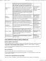
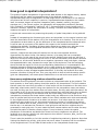
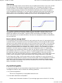
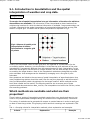
Chapter13 - CM Box User Guide
1 of 9
http://80.69.76.153/wiki/index.php?title=Chapter13&printable=yes
5.1. Introduction to Geostatistics and the spatial
interpolation of weather and crop data.
By Jürgen Grieser
The major aim of spatial interpolation is to get information of locations for which no
observations are available. The information is then interpolated to these locations from
neighbouring locations for which the desired information is available. In agrometeorology one
is usually interested in the spatial interpolation of meteorological data as well as crop yield
data on a regular grid. The basic idea of spatial interpolation is depicted in Fig 1.
Fig.1: Scheme of spatial point
interpolation of station
information to a regular grid
of points.
Usually the interpolated values at each grid point are regarded as representative for the
surrounding square. However, one should keep in mind that the point estimate of the point
interpolation is conceptually different from the area estimate of a block interpolation. In the
latter case the target is not the value of a single location, but the area average of the square
surrounding the target location. Most of the interpolation methods are designed to provide
point estimates. Area averages can be obtained by averaging over a fine grid of point
estimates.
Many questions are linked to the vast area of spatial interpolation of agroclimatic data. How
many neighbouring stations should be used? How far may they be away to add information?
How to mathematically obtain the estimate for the target location? Which methods are the
best? How reliable are the results? The following sections aim to answer part of these
questions and demonstrate how New_LocClim, the interpolation tool within the CM Box, solves
the according problems.
Which methods are available and what are their
properties?
There is quite a variety of interpolation methods ranging from very simple and easy-to-use
ones to very sophisticated strategies taking into account lots of supplementary information.
The variety of methods can be grouped with respect to certain features in order to easily get
an idea of what they provide. The grouping criteria and their meanings are explained in Tab.
1.
Tab. 1: Grouping criteria for interpolation methods, short explanation and examples.
Criteria
Explanation
Example
11/14/2006 3:37 PM
Chapter13 - CM Box User Guide
2 of 9
http://80.69.76.153/wiki/index.php?title=Chapter13&printable=yes
Scale free vs.
scaled
A scale free method does not recognize the size of
the system. Scale free methods do not distinguish
the case where one station is 10m and the other
30m away from the case where one station is 100km
and the other is 300km away. However, from an
agroclimatical point of view there is a tremendous
difference which should be taken into account.
Scaled methods often use a scale parameter. If the
chosen scale parameter is too large local variations
are smoothed out. If it is too small, the information
that may be contributed by stations further away is
practically ignored.
Inverse distance
interpolation is
scale free.
Shepards method
is scaled.
Exact vs.
smoothing
What happens if the target location falls exactly on
the location of a station? An exact method would
reproduce the observations. Smoothing methods
take the observations of other locations into account
and lead to a more averaged estimate.
Inverse distance
interpolation is
exact. Modified
inverse distance
interpolation is
smoothing.
If the user has not to provide any parameter to
Parameter free vs.
interpolate (and the method does not use built-in
with parameters
parameters) the method is called parameter free.
Nearest neighbour
interpolation is
parameter free.
Continuous
vs.dsicontinuous
If for any 2 locations the interpolated values
converge if the locations converge then the method
is called continouos.
Nearest neighbour
interolation is
discontinuous.
Global polynomials
are continuous.
Local vs. global
A method that takes all stations into account for
each target location is called global. If it uses only
part of the stations it is more or less local. Each
method can be ‘localized’ by limiting the distance of
stations to the target location or the number of
stations to be used.
Nearest neighbour
interpolation is the
most local.
Extrapolating vs.
non-extrapolating
A method is called non-extrapolating if the range of
interpolated values does not exceed the range of
observed values.
Kriging is
extrapolating,
inverse distance
averaging not.
Geostatistical Interpolation Methods
Which method is the best?
There is no best method. You have to find the most adequate method with respect to the data
given, station density and distribution, geographic conditions, season, degree of temporal
integration (i.e. daily, decadal, monthly data) etc.
This is why the geostatistical methods which are available within the CM Box are described
here in more detail.
Nearest Neighbour
Scale free, exact, parameter free, discontinuous, local, non-extrapolating
This is by far the simplest method of spatial interpolation. For each grid point the value of the
nearest station is taken.
Inverse Distance Weighted Averaging (IDWA)
Scale free, exact, 1 parameter, continuous with singular points, global, non-extrapolating
11/14/2006 3:37 PM
Chapter13 - CM Box User Guide
3 of 9
http://80.69.76.153/wiki/index.php?title=Chapter13&printable=yes
IDWA is an averaging procedure. It gives each neighbouring station a weight which is
proportional to a power of the inverse of the station distance. Thus, closer stations have more
weight in the averaging procedure than stations that are further away. If the power exponent
is large, closer stations get much more weight than stations that are further away. Therefore,
with an increasing power exponent, IDWA converges to nearest neighbour interpolation. On
the other hand, the smaller the exponent is, the further reaches the influence of each station.
For exponents close to zero, the interpolated field becomes the area average with narrow
spikes at station locations. Note that if a station is very close to the grid point it gets nearly all
the weight. If a grid point and station are at exactly the same location IDWA is not defined
because of division by zero. However, this is not a problem as in the very close vicinity of a
station IDWA can be replaced by nearest neighbour interpolation.
Modified IDWA
Scale free, smoothing, 2 parameters, continuous, global, non-extrapolating
One of the disadvantages of IDWA is that the influence of the closest station becomes rather
high if this station is very close to the grid point compared to the other stations of the
neighbourhood. This leads to the circus-tent like form of the interpolated field. In order to
avoid this, Modified IDWA adds a displacement to each station distance. This means that even
in the close vicinity of a station, this station does not get most of the weight, so the
interpolated surface becomes smoother and the singular points (station locations) vanish.
However, Modified IDWA is no longer an exact interpolation routine.
Cressmanns Method
Scaled, smoothing, 2 parameters, discontinuous, local, non-extrapolationg
Cressmanns Method avoids some of the shortcomings of IDWA. Only stations within a circle
around the grid point are used for the interpolation. Within this circle the weights of the
stations depend on the distance from the grid point. A pre-given weight function, which stays
high in the close vicinity of the grid point and becomes steeper with increasing distance and
finally smoothly approaching zero, ensures that the weights are distributed with respect to a
scale. This is a considerable advantage compared to IDWA. However, the radius of the circle
has to be described, and the scale is fixed. If the radius is smaller than the closest station at a
grid point the method gives no result. If the radius is large, the finer details of the
climatological field may be smoothed out. Thus this method is not recommended where there
are groups of stations with large gaps between them (a condition which is quite common in
arid areas).
A modified version of Cressmanns Method allows the range to be broadened where the
Cressmanns weights are high. This is done by an exponent. The higher it is, the higher is the
weight of the stations further away compared to the closer ones.
Structure Function
Scaled, smoothing, n parameter, continuous, global, non-extrapolating
The disadvantage of Cressmanns method is that stations outside the pre-given circle are not
taken into account. Structure Functions avoid this disadvantage and simultaneously use the
advantage of a pre-given scale. This means that if the neighbouring stations are all far away
with respect to the scale they all get nearly the same weight. The point is that none of the
far-away neighbours is considered to contain much more information about the local
conditions than any of the others. However, the problem with this method is that the user has
to provide a scale parameter.
Many monotonic functions can be used as Structure Functions. Within CM-Box two are
provided: a Gaussian and an exponential. With the first, the influence of a station decreases
over distance in a bell shape. The scale parameter gives the distance at which the power
decreases to half its value. With the second structure function, the influence decreases
exponentially. The scale parameter gives the distance at which the power of the station
decreases to 1/e (about 0.368) of its initial power of 1.
11/14/2006 3:37 PM
Chapter13 - CM Box User Guide
4 of 9
http://80.69.76.153/wiki/index.php?title=Chapter13&printable=yes
The advantage that Cressmanns method and Structure Functions have in common is that one
knows exactly (or at least one can know) which part of the spatial high frequency variability is
suppressed.
Polynomials
Scale free, smoothing, nonparametric, discontinuous, local, extrapolating
This interpolation method is completely different from the previous ones. It fits a
deterministic, two-dimensional function to the observations given by the neighbouring
stations. The function value at the grid point represents the interpolated value. Since the
function parameters are determined by a least-squares fit, it is by definition a smoothing
method. Its smoothness depends on the number of neighbours which are used for the fit. It
gives reasonable results with a high station density and in case of poor accuracy in the
observed values. It has no scale property. Its major disadvantage is that if all the
neighbouring stations are grouped to one side of the grid point the estimated value becomes a
(non-linear) extrapolation of the local horizontal trend. Thus the estimates at the borders of a
map may not be at all reliable.
Shepards Method
Scaled, exact, several parameters, discontinuous, local, non-extrapolating
Shepards method is especially designed for climate interpolation. First a circle is drawn around
the grid point containing, on average, seven stations. If there are less than four or more than
ten stations within the circle the radius is changed so that the fifth nearest or the eleventh
nearest station lies on the frame of the circle. This procedure ensures that the length scale is
taken as a constant if possible. Only in regions with very high or very low station density the
scale is changed to keep the number of stations used for the interpolation between four and
ten. Within the circle a weight function is applied which monotonically decreases with the
radius. In the next step the weights are altered with respect to directional isolation of the
stations. This step is like a simple shadow correction. Since the weight function itself is like
inverse distance weighted averaging in the close vicinity of a grid point, it would lead to
singular points if a grid point and a station location coincide. Even if they do not coincide but
lay close together, the grid point may become an unreasonable local maximum or minimum
just because the closest station has an extraordinarily high weight. This situation is avoided by
using a small local average-gradient correction. Finally, if one or more stations are very close
to a grid point the simple average of these stations is taken as the interpolated value.
One advantage of Shepards Method is that it runs completely automatically. No parameters
have to be set to obtain results. It automatically takes station density and grid size into
account.
Kriging
Scales adapt automatically, smoothing, parameter free, continuous, global, extrapolating
The basis of Kriging is a probabilistic concept with the following assumptions:
The variable is random in space,
Invariance of translation,
Invariance of rotation.
Based on these assumptions a variogram is calculated. It gives the mean squared difference in
the observed values as a function of the distance between the locations of observations. It can
be shown that the estimate for the grid point can be expressed as a linear combination of the
surrounding observations with weights following from the variogram. With the conditions given
above the estimates are ‘blue’ (best linear unbiased estimators). This means that no other
linear interpolation technique gives better results on average (smaller root mean square
error). However, the above given assumptions mean that
the variable should be stochastic only with no deterministic part in it,
11/14/2006 3:37 PM
Chapter13 - CM Box User Guide
5 of 9
http://80.69.76.153/wiki/index.php?title=Chapter13&printable=yes
it makes no difference for the spatial correlation where you are,
direction does not matter.
Only if these conditions are fulfilled, it be shown that simple Kriging leads to ‘blue’ results.
Apart from simple Kriging, many variations of the method exist. One of them is Co-Kriging
where another variable is taken into account. This can be either another climatological variable
or any other reasonable one, e.g. altitude. Satellite Enhanced Data Interpolation (SEDI) is a
special application of Co-Kriging. It uses the spatial pattern of satellite images of cold cloud
top duration for the interpolation of tropical precipitation fields.
Thin-Plate Splines
Scale free, exact, parameter free, continuous, global, extrapolating
Thin-Plate Splines is a special kind of radial basis function. It can be seen as a deterministic
method with a local stochastic component. The main condition is the minimum of curvature of
the deterministic part. Another condition is that the interpolated surface has to meet the
observations.
Also Thin-Plate Splines comes in a variety of versions. The deterministic part can be any
arbitrary function. The so called smoothing Thin-Plate Splines allow a smoothing parameter to
decide how strong the influence of the local stochastic part is. Note that minimization of
curvature may lead to unreasonable extrapolations of local horizontal climate trends at the
margins of the map.
Deterministic structures
Aside the stochastic part of agroclimatic variables there is the deterministic fraction which can
be rather developed. The fraction of spatial variance of a variable that can be attributed to
deterministic structures varies from variable to variable and with respect to the degree of
integration. In the extreme case of long-term averages of monthly mean temperatures the
overwhelming majority of spatial variability within hundreds of kilometers may be explained by
altitude alone. There may also be a clear horizontal gradient. Before interpolating agroclimatic
data it should be analysed which fraction of variance is explained by either vertical or
horizontal gradients. If they explain a considerable fraction of variance they should be treated
separately as explained in the following subsections.
Altitude Correction
Either a look on the observation-altitude graph or a look on the explained fraction of variance
by altitude (or both) clarifies whether altitude matters or not. If it matters it should be taken
into account by transforming the observations via linear regression to values that would have
been observed at the station location if it had the same altitude as the target location. Then,
in a second step the spatial interpolation of the pre-transformed observations may be
performed. Aside an improvement of the interpolation this yields to an understanding of the
effect on altitude on the variable under consideration. However, several problems may arise in
data sparse areas with altitude regression. They are discussed in the section Warnings.
Horizontal Gradients
Some of the interpolation methods take deterministic spatial structures into consideration
(polynomials, thin-plate splines). The easiest possible spatial structure is a horizontal gradient
(trend), and if the region which is covered by the neighbourhood of stations is small enough,
even more complicated regional spatial structures may be well approximated by local planes.
Therefore, we suggest local gradients to be taken into consideration in the same way as is
done with the altitude correction.
However, we not recommend to apply horizontal and altitude regression in one step since both
can be collinear and a strange and meaningless mixture may follow. If both altitude and
horizontal gradients should be applied, we suggest dealing with them separately. This means,
that first the altitude dependency should be approximated and then the horizontal gradients.
11/14/2006 3:37 PM
Chapter13 - CM Box User Guide
6 of 9
http://80.69.76.153/wiki/index.php?title=Chapter13&printable=yes
How good is spatial interpolation?
The quality of spatial interpolation of agroclimatic data depend on the station density, station
distribution and the spatial representativeness of the observed variable. The
representativeness may be expressed in a scale length which is the distance of two stations
which have half of their variability in common. Representativeness depends on the variable
itself, the season, degree of temporal integration (daily, decadal, monthly, long term
averages, etc.), the climatic regime, the geographic and topographic conditions (flat land,
hills, mountains, continentality, maritimity, etc.). Some estimates of scale lengths exist in
literature. However, usually this information is missing. Therefore one needs another way to
measure the quality of interpolation.
A simple and conservative way measuring the quality of spatial interpolation is the jackknife
error.
Instead of interpolating the climate at grid points we interpolate it to the station locations and
leave the observation at the station out for the interpolation at its location. Then the error of
interpolation at each station is just the difference of the interpolated and the observed value.
It can be seen as a property of the station with respect to the method used and the
neighbouring stations. Averaging all these station-based errors leads to an estimate of the
interpolation bias. The sum of squared deviations from this bias gives an average
station-based error.
However, imagine the case where all stations but one are close together and their
observations are rather similar. One station however, is far away and has a completely
different value. In this case all but one will have a small Jackknife error and one will have a
large one. Should we simply average the errors? If we are interested in area specific answers
we should not. All the small Jackknife errors together represent a small sub-region, whereas
the separated station may represent the major part of the total area. Thus the averaging
should include the region for which the corresponding Jackknife error is representative. We
therefore suggest to attribute a jackknife error to each gridpoint by nearest neighbour
interpolation and to average afterwards over all gridpoints to get an area averaged Jackknife
error as well as an area averaged standard deviation. In this way the Jackknife error also
becomes a function of the grid size. Thus, one may whish to look at both the station specific
(grid size independent) root mean square Jackknife error as well as the area specific one.
How many neighbouring stations should be used?
The stations around a gridpoint are used to obtain an interpolated value at the gridpoint. The
basic question is: How many stations should be used for the interpolation? The more stations
that are used, the more likely the effect of a local outlier will be smoothed out. But does more
data really mean better results? Using more stations for the interpolation means more data
are used, but they are from stations that are further away. Do they really add information? Do
they matter at all? Or do they worsen the results because they add information from a distant
location? Some methods give the stations that are further away much less weight in the
interpolation procedure thus these stations make hardly any difference to the results so using
them is optional and little more than a waste of time. Other methods exist which automatically
fix the neighbourhood of stations to be taken into account. In all other cases the user can
decide how many stations to use. We suggest to keep the number of neighbouring stations
small. The default value of New_LocClim is 10. This sounds low, but one should bear in mind
that the aim is to estimate the climate at a local grid point and that this neighbourhood is
generated for each grid point. In some cases the tenth nearest station can be rather far away
and add information of another climate regime. It may be best to look at the spatial
distribution of the stations and decide from there how many neighbours are optimal. The
Jackknife error can be a helpful tool with respect to this decision. However, New_LocClim can
deal with up to 100 neighbours.
There is also the possibility to limit the number of neighbouring stations by distance. Note that
limiting the distance too strictly, grid points may occur where no stations fulfil the conditions
of the neighbourhood. This will lead to blank areas on the interpolated climate map.
11/14/2006 3:37 PM
Chapter13 - CM Box User Guide
7 of 9
http://80.69.76.153/wiki/index.php?title=Chapter13&printable=yes
Shadowing
Seen from the target location some stations may be hidden behind others. They may not add
new information of the climate at the target location. Fig. 2 illustrates the effect of such
groups of stations. Pure distance weighting methods are prone to these situations. Therefore
in case of large grouping of stations one should either eliminate some of them to obtain a
more homogeneous distribution or one may apply a shadowing that gives less weight to the
stations which are in the shadow of others. Kriging methods automatically take care of this
effect and can not be improved by shadowing. This is one of the strengths of kriging.
a)
b)
Fig. 2. Effect of stations behind other stations on the interpolation surface. Black lines are
interpolation results if only 4 stations (black triangles) are used. In penal a) three more
stations are added on the left side, in panel b) three more stations are added on the right
side. These stations do not add information, but alter the interpolation results as sketched by
the coloured lines.
How to detect strange data?
If one assumes that the observed values for each month are the sum of a horizontal function,
a vertical function, and random noise one can detect outliers. As a first step all data may be
reduced to the same altitude and location by the functions fitted to the data. In the next step
the value furthest away from the average is assumed to be an outlier and thus extracted to
obtain unbiased average and variance of the residual ensemble. The latter can be used to
calculate thresholds which are exceeded very rarely by chance. If the probability to exceed a
threshold in one trial is given as q and one assumes independent trials (i.e. independent
observations at the neighbouring stations) than one can apply a Poisson model to calculate
the probability that one in n trials (n= number of neighbouring stations) is as far away from
the observed average as the assumed outlier is. If this probability is less than a certain
threshold (10% say) the observation should be regarded as strange. In the single point mode
of New_LocClim the station, month and variable of the strange observation is provided.
In the map mode of New_LocClim each station can be a neighbour for many grid points. It
may provide strange data with respect to some of these cases. Thus, strangeness of a station
is provided in this case as the ratio of cases where the station seemed to provide strange
data. The results are provided in the sub menu manually of the menu item stations and as
station information on the map.
A practical guide
As a general strategy for the interpolation of agroclimatic data we recommend to first
investigate the data in order to answer the following questions:
1. Do I have enough data?
This can be recognized by an acceptable Jackknife error.
2. Is the station distribution acceptable?
Draw a map of the station locations. If you see large gaps come to think of it. Do they
11/14/2006 3:37 PM
Chapter13 - CM Box User Guide
8 of 9
http://80.69.76.153/wiki/index.php?title=Chapter13&printable=yes
matter? Is there any peculiarity with the gaps (e.g. a mountain range)? In this case one
should not simply interpolate over the gap but try to close it by obtaining data from the
area affected. Do not forget to care for the marginal areas. Try to obtain and take into
account stations surrounding your area of interest in order to get reliable results also at
the margins of the map.
3. Are there strange data?
Draw the observations in a map either as values or as coloured points. Outliers become
visible this way. But be careful. Sometimes the only mountain station on a map provide
valuable information since the observation is quite different from the observation at all
other stations. This does not mean that it is an outlier. Use the strange data warning of
New_LocClim. Drop obviously wrong values.
4. Do the data depend on altitude?
Draw a map of explained variances by altitude regression and a map of regression
coefficients (slopes). If the explained variance is high and the regression coefficients are
meaningful then apply altitude regression before applying geostatistical methods. The
maps of explained variances and regression coefficients are valuable agroclimatic
information. Experiment with the number of stations used to calculate local correlation
and regression coefficients.
5. Do the data show a horizontal gradient?
This can be checked in the same way as the altitude dependency. If it is important it
should be taken into consideration. Clarify which geostatistical interpolation method to
prefer and find the optimal parameter values.
6. Do the stations cover the whole range of altitude of the grid points?
The altitude range covered by the stations should cover the range of altitude of the grid
points. Otherwise the interpolation is in fact an altitude extrapolation. An altitude
observation plot helps to see whether this is a problem. Truncated altitude regression
may avoid altitude extrapolation. Maps of local altitude extrapolation may be drawn.
Clarify which geostatistical interpolation method to prefer and find the optimal
parameter values.
7. Is any of the grid points lonely?
If the group of neighbouring stations does not surround the target location but falls at
one side of it, the target location may called lonely and the interpolation to it may be
seen as a horizontal extrapolation. A map of horizontal extrapolation warning may be
drawn to clarify this.
8. Clarify which geostatistical interpolation method to prefer and find the optimal parameter
values.
Some methods are based on featuers which are les adequate withrespect to some
variables. AS an example thin-plate splines minimizes curvature. The spatial field of
precipitation however may have regions with high curvature and steep gradients. Large
precipitation and no precipitation may be in within very close vicinity. Therefore one
might expect that thin-plate splines is not the optimal method for the interpolation of
precipitation. However, superior to the theoretical investigations of this kind is trial and
error. The method with the least Jackknife error and reasonable interpolated maps
should be used. In order to estimate Jackknife errors, it is not necessary to do all the
interpolations with the final resolution. Therefore this investigation may be less time
consuming as one expects. Note that Jackknife errors of smoothing methods are usually
lower compared to exact methods. Experiment with the number of stations used to
calculate local correlation and regression coefficients.
11/14/2006 3:37 PM
Chapter13 - CM Box User Guide
9 of 9
http://80.69.76.153/wiki/index.php?title=Chapter13&printable=yes
Retrieved from "http://80.69.76.153/wiki/index.php?title=Chapter13"
This page has been accessed 467 times. This page was last modified 09:33, 4 October 2006.
11/14/2006 3:37 PM