Download Planet Simulator User's Guide

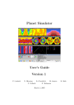
Planet Simulator
User’s Guide
F. Lunkeit
U. Luksch
K. Fraedrich
H. Jansen
F. Sielmann
K. Cassirer
M. Lob
M. Preuhs
December 17, 2003
E. Kirk
W. Joppich
2
Contents
1 Installation
5
1.1
Quick start . . . . . . . . . . . . . . . . . . . . . . . . . . . . . .
5
1.2
Unpacking and installation . . . . . . . . . . . . . . . . . . . . . .
6
1.3
Compiling and running PUMA . . . . . . . . . . . . . . . . . . .
8
1.3.1
pumaburner . . . . . . . . . . . . . . . . . . . . . . . . . .
9
1.4
Intel FORTRAN compiler . . . . . . . . . . . . . . . . . . . . . .
10
1.5
Absoft FORTRAN compiler . . . . . . . . . . . . . . . . . . . . .
10
2 Modules
11
2.1
fluxmod.f90 . . . . . . . . . . . . . . . . . . . . . . . . . . . . . .
13
2.2
miscmod.f90 . . . . . . . . . . . . . . . . . . . . . . . . . . . . . .
14
2.3
surfmod.f90 . . . . . . . . . . . . . . . . . . . . . . . . . . . . . .
15
2.4
mod.f90 . . . . . . . . . . . . . . . . . . . . . . . . . . . . . . . .
16
2.5
Files . . . . . . . . . . . . . . . . . . . . . . . . . . . . . . . . . .
17
2.6
guimod.f90 . . . . . . . . . . . . . . . . . . . . . . . . . . . . . . .
18
2.7
Sea ice and ocean modules . . . . . . . . . . . . . . . . . . . . . .
19
2.7.1
seamod.f90
. . . . . . . . . . . . . . . . . . . . . . . . . .
23
2.7.2
intermodatm.f90 . . . . . . . . . . . . . . . . . . . . . . .
24
2.7.3
intermodice.f90 . . . . . . . . . . . . . . . . . . . . . . . .
25
2.7.4
icemod.f90 . . . . . . . . . . . . . . . . . . . . . . . . . . .
26
2.7.5
oceanmod.f90 . . . . . . . . . . . . . . . . . . . . . . . . .
27
2.7.6
oceanmod50.f90 . . . . . . . . . . . . . . . . . . . . . . . .
28
3
4
CONTENTS
3 Running PUMA
29
3.1
Interactive Console Mode . . . . . . . . . . . . . . . . . . . . . . .
29
3.2
Batch Mode . . . . . . . . . . . . . . . . . . . . . . . . . . . . . .
30
4 Graphical User Interface
4.0.1
Introduction . . . . . . . . . . . . . . . . . . . . . . . . . .
37
4.0.2
Installing the PlaisirGUI . . . . . . . . . . . . . . . . . . .
37
4.0.3
Operating . . . . . . . . . . . . . . . . . . . . . . . . . . .
40
4.0.4
Trouble Shooting . . . . . . . . . . . . . . . . . . . . . . .
51
4.0.5
Additional Tools . . . . . . . . . . . . . . . . . . . . . . .
52
5 Postprocessing
5.1
37
55
Pumaburner . . . . . . . . . . . . . . . . . . . . . . . . . . . . . .
55
5.1.1
Introduction . . . . . . . . . . . . . . . . . . . . . . . . . .
55
5.1.2
Usage . . . . . . . . . . . . . . . . . . . . . . . . . . . . .
56
5.1.3
Namelist . . . . . . . . . . . . . . . . . . . . . . . . . . . .
56
5.1.4
Format of output data . . . . . . . . . . . . . . . . . . . .
58
5.1.5
SERVICE format . . . . . . . . . . . . . . . . . . . . . . .
59
5.1.6
HHMM . . . . . . . . . . . . . . . . . . . . . . . . . . . .
59
5.1.7
HEAD7 . . . . . . . . . . . . . . . . . . . . . . . . . . . .
59
5.1.8
MARS . . . . . . . . . . . . . . . . . . . . . . . . . . . . .
60
5.1.9
MULTI . . . . . . . . . . . . . . . . . . . . . . . . . . . .
60
5.1.10 Namelist example . . . . . . . . . . . . . . . . . . . . . . .
60
5.1.11 Troubleshooting . . . . . . . . . . . . . . . . . . . . . . . .
61
6 Graphics
63
6.1
Grads . . . . . . . . . . . . . . . . . . . . . . . . . . . . . . . . .
63
6.2
Vis5D . . . . . . . . . . . . . . . . . . . . . . . . . . . . . . . . .
67
Bibliography
68
CONTENTS
A List of Constants and Symbols
A.0.1 List of Constants and Symbols . . . . . . . . . . . . . . . .
B Puma Codes
5
69
70
75
6
CONTENTS
Chapter 1
Installation
1.1
Quick start
This section is for the very unpatient, used to skip manuals and just eager to see
results as fast as possible. The quick start just guides you till the first data output
is produced. The next steps, the post processing and the graphical presentation
are described in chapter 5+6. For a more detailed description of what this package
is all about, read the paragraph following this quick start.
• type ”mkdir plasim”
• type ”cp plasim.tar plasim”
• type ”cd plasim”
• type ”tar -xvf plasim.tar”
• type ”mkdir run”
• type ”cd module”
• type ”make”
• type ”cp puma.x ../run”
• type ”cd ..”
• type ”cp puma.x run”
• type ”cp data/* namelist data/* parameter run”
• type ”cd run”
7
8
CHAPTER 1. INSTALLATION
• type ”puma.x”
You may need to adjust the Makefile to your environment, in particular the
fortran-compiler command and the c-compiler command. The last step may take
a while to be finished, depending on your maschine’s processing speed. After all
you should find four output files: puma output, puma restart, land restart and
sea restart. Further information on how to run puma is given in chapter 4. The
file puma output contains the model results and has to be postprocessed using
”pumaburn4” (see chapter 5). The restart files contain information neccessary
to restart the model run from the end of the current integration.
1.2
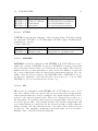
Unpacking and installation
This chapter briefly describes which files are included, how to install the package and which steps have to be taken for a first run. The file plasim.tar includes PUMA-module files, data and namelist files to run PUMA, some additonal
programs for postprocessing (e.g. afterburner), some scripts, a Makefile and a
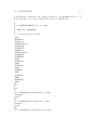
README.txt. All files are listed below with a short description. After unpacking the tar-file in a suitable directory with the command ”tar -xvf plasim.tar”
you should find the following files:
PUMA-Modules
============
file
---fftmod.f90
fluxmod.f90
landmod.f90
legmod.f90
miscmod.f90
mpimod.f90
mpimod_dummy.f90
description
----------: fast fourier transformation
: boundary layer fluxes and vertical diffusion
(surface fluxes of heat and momentum, vertical
diffusion of temperature, moisture and momentum)
: land-surface and soil processes (soil temperature
soil water, snow cover and snow temperature, river
runoff, vegetation)
: legendre transformation
: miscellaneous (correction of negative humidity)
: interface to MPI
: dummy routines substituting the MPI-routines
(for use on scalar-machines instead of mpimod.f90)
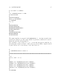
1.2. UNPACKING AND INSTALLATION
outmod.f90
pumamod.f90
puma.f90
radmod.f90
rainmod.f90
seamod_climatology.f90
surfmod.f90
9
: output
: module for global variables (to be used in other
modules)
: atmospheric main programm and dynamic
: radiation (long- and short-wave)
: moist processes (large-scale and convective
precipitation cloud cover)
: climatological sea surface (ocean and sea ice)
: interface to surface modules (sea and land)
Data
====
file
---surface_parameter
description
----------: initial fields and climatologies
(orography, land-sea mask, glacier mask
surface temperature, sea ice cover)
(AMIP-SSTs are used for this climatology)
Namelists
=========
file
---puma_namelist
land_namelist
sea_namelist
description
----------: example namelist for puma (typical set up)
: example namelist for landmod.f90
: example namelist for seamod_climatology.f90
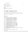
Scripts and Makefile
====================
file
----
description
-----------
10
CHAPTER 1. INSTALLATION
Makefile
compile_mpp
runscript_template
: makefile to compile PUMA (scalar machine)
: script to compile PUMA for MPI (see NPRO in
PUMAMOD.f90!)
: example script to run PUMA for some years (unix)
Additional
==========
file
----
description
-----------
pumaburn4.c
srv2gra.f90
srv2ascii.f90
PumaGui-install.tar.gz
PumaGui-doc.pdf
README-0.2.1
1.3
: pumaburner with netcdf export support (compile with
standard c-compiler, e.g. cc -O2 -o pumaburn4
-D_FILE_OFFSET_BITS=64 pumaburn4.c -lm -lnetcdf)
: convert service format (typical afterburner output)
to grads input (control and data)
compile it with FORTRAN90 compiler
usage: srv2gra INPUT will create an INPUT.ctl and
an INPUT.gra file. Open INPUT.ctl using GRADS
(on some machines you have to modify the record
length)
: converts service format model output to its ascii
representation presently using the fortran format
"8I10" for the header and the format "8E12.6" for
the data
: graphical User Interface for PLASIM (see Chapter 4)
: documentation for the graphical user interface
: README for the graphical user interface
Compiling and running PUMA
To compile PUMA you may take these steps:
• use ”make” for compiling a set of modules. Just type ”make” in the module
directory and the executable ”puma.x” will be created.
• The utilities ”pumaburn” and ”srv2gra” need to be compiled separately.
The package pumaburn2.tar.gz contains a Makefile, which might have to be
1.3. COMPILING AND RUNNING PUMA
11
customized before invocation. The program ”srv2gra.f90” only needs to be
compiled with any FORTRAN90 compiler, (e.g. f90 -o srv2gra srv2gra.f90).
After compiling, create a directory (e.g. ”run”) and copy the executable puma.x,
all initial fields (* parameter) and the namelists (* namelist) into it. Addtionally you can run PUMA on maschines with more than one processor, using the
compile mpp script (see file list). The latter needs the message passing interface
(MPI) to be installed properly. This package doesn’t include MPI, but it can be
downloaded from many sites:
(e.g. http://www.go.dlr.de/fresh/unix/src/misc/mpich-1.2.4.tar.gz)
Run the PUMA executable by either:
1. using a script like the runscript template example script (which has been
tested on linux but may also work on other unix machines)
2. just typing ”puma.x” in the run directory
3. creating your own run setup (examples are given in chapter 4.2)
A detailed description of model parameters to be defined in the namelists can be
found in chapter 3.
Finally, analyse the output using the ”pumaburn4” program together with your
own software. If you like to plot some results, you may use the ”srv2gra” program,
which converts the output to a format suitable for GrADS (see chapter 6).
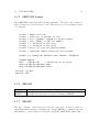
1.3.1
pumaburner
As mentioned above, using the postprocessor ”pumaburner4” is highly recommended for extracting variables and levels from the raw packed puma data (file:
puma data). On platforms other then linux build the executable by just invoking a standard c-compiler, (e.g. cc -O2 -o pumaburn4 pumaburn4.c -lm
-lnetcdf). In case that netCDF output is not wanted or the netCDF library isn’t
available, please change the line ”#define NETCDF OUTPUT” into ”#undefine
NETCDF OUTPUT” within the source and omit binding the netCDF library ”lnetcdf” at compile time. When compiling the postprocessor under linux, please
add the following option to the compile command: ”-D FILE OFFSET BITS=64”.
This enables the handling of files > 2 GByte, which is still a hard limit under
older linux kernels (< 2.4.20). For a detailed description of the pumaburner, see
chapter 5.
12
1.4
CHAPTER 1. INSTALLATION
Intel FORTRAN compiler
The PUMA model is tested with various brands of fortran compilers. There is
no special care to be taken when compiling it. On default the INTEL compiler
enables normal optimization (-O2), which should be sufficient and even recommended for the model to run. For your convenience just use the included Makefile
for compiling, see former sections.
In case of compiling the included tools, such as ”srv2gra”, you have to add the
compiler option ”-Vaxlib”. This enables the compiler to find the non-standardfortran features, such as ”getarg, iarg, etc ...”
1.5
Absoft FORTRAN compiler
This compiler should work well with PUMA. Just use the Makefile and watch
PUMA being built, see former sections. The default for optimization is none.
The recommended level is ”-O1”, which corresponds to basic optimization. This
is sufficient for most applications. Please change the Makefile accordingly or
compile PUMA manually. The next level of optimization may rearrange your code
substantially including strength reduction, loop invariant removal, code hoisting,
and loop closure. This is neither usable with debugging options nor together with
the message passing interface !
In case of compiling the included tools, such as ”srv2gra”, you have to add the
unix compatibility library libU77 via ”-lU77”. This enables the compiler to find
the non-standard-fortran features, such as ”getarg, iarg, etc ...”
Chapter 2
Modules
This is a technical documentation of the PUMA-II model. In the following, the
purposes of the individual modules is given and the general structure and possible
input and output opportunities (namelist, files) are explained.
13
14
CHAPTER 2. MODULES
15
2.1
fluxmod.f90
General The module fluxmod.f90 contains subroutines to compute the different surface fluxes and to perform the vertical diffusion. The interface to the
main PUMA module (puma.f90, see ...) is given by the subroutines fluxini,
fluxstep and fluxstop which are called in puma.f90 in the subroutines prolog,
gridpointd and epilog, respectively.
Input/Output fluxmod.f90 does not use any extra input file or output file and
is controlled by the namelist fluxpar which is part of the puma.f90 namelist file:
Parameter
NEVAP
Type
Integer
NSHFL
Integer
NSTRESS
Integer
NVDIFF
Integer
VDIFF LAMM
Real
VDIFF B
Real
VDIFF C
Real
VDIFF D
Real
Purpose
Switch for surface evaporation (0
= off , 1= on)
Switch for surface sensible heat
flux (0 = off , 1= on)
Switch for surface wind stress (0
= off , 1= on)
Switch for vertical diffusion (0 =
off , 1= on)
Tuning parameter for vertical diffusion
Tuning parameter for vertical diffusion
Tuning parameter for vertical diffusion
Tuning parameter for vertical diffusion
Default
1
1
1
1
160.
5.
5.
5.
Structure Internally, fluxmod.f90 uses the FORTRAN-90 module fluxmod,
which uses the global common module pumamod from pumamod.f90. Subroutine fluxini reads the namelist and, if the parallel version is used, distributes
the namelist parameters to the different processes. Subroutine fluxstep calls
the subroutine surflx to compute the surface fluxes and calls the subroutine
vdiff to do the vertical diffusion. Subroutine fluxstop is a dummy subroutine since there is nothing to do to finalize the computations in fluxmod.f90.
The computation of the surface fluxes in surflx is spitted into several parts.
After initializing the stability dependent transfer coefficients, the subroutines
mkstress, mkshfl and mkevap are the computations which are related to the
surface wind stress, the surface sensible heat flux and the surface evaporation,
respectively.
16
2.2
CHAPTER 2. MODULES
miscmod.f90
General The module miscmod.f90 contains miscellaneous subroutines which
do not fit well to other modules. The interface to the main PUMA module
(puma.f90, see ...) is given by the subroutines miscini, miscstep and miscstop
which are called in puma.f90 in the subroutines prolog, gridpointd and epilog,
respectively. A subroutine to eliminate spurious negative humidity and an
optional subroutine for dry convective adjustment is included in miscmod.f90.
Input/Output miscmod.f90 does not use any extra input or output file and
is controlled by the namelist miscpar which is part of the puma.f90 namelist
file:
Parameter
Type
Purpose
default
NDCA
Integer
Switch for convective adjustment 0
(0 = off , 1= on)
Structure Internally, miscmod.f90 uses the FORTRAN-90 module miscmod,
which uses the global common module pumamod from pumamod.f90. Subroutine miscini reads the namelist and, if the parallel version is used, distributes
the namelist parameters to the different processes. Subroutine miscstep calls
the subroutine fixer to eliminate spurious negative humidity arising from the
spectral method and, if dry convection is switched on, calls the subroutine
mkdca to do the dry convective adjustment. Subroutine miscstop is a dummy
subroutine since there is nothing to do to finalize the computations in miscmod.f90.
17
2.3
surfmod.f90
General The module surfmod.f90 deals as an interface between the atmospheric part of the model and modules, or models, for the land and the oceans.
The interface to the main PUMA module (puma.f90, see ...) is given by the
subroutines surfini, surfstep and surfstop which are called in puma.f90 in the
subroutines prolog, gridpointd and epilog, respectively. Calls to subroutines
named landini, landstep and landstop and seaini, seastep and seastop provide
the interface to land and the ocean modules , respectively.
Input/Output surfmod.f90 reads the land-sea mask and the orography from
the surfaceparameter file (see puma...). surfmod.f90 is controlled by the
namelist surfpar which is part of the puma.f90 namelist file:
Parameter
Type
Purpose
default
NSURF
Integer
Debug switch
not active
NOROMAX
Integer
Resolution of orography
NTRU
OROSCALE
Real
Scaling factor for orography
1.
Structure Internally, surfmod.f90 uses the FORTRAN-90 module surfmod,
which uses the global common module pumamod from pumamod.f90. Subroutine surfini reads the namelist and, if the parallel version is used, distributes
the namelist parameters to the different processes. If the run is not started
from a restart file (NRESTART from namelist inp is 0), the land-sea-mask
and the orography is read from the surfaceparameter file. According to
the namelist input, the orography is scaled by OROSCALE, transfered into
spectral space and truncated to NOROMAX. Calls to subroutines landini and
seaini are the interfaces to the respective initialization routines contained in
the land and ocean modules. During the run, the interface to land and ocean
is given by calls to the external subroutines landstep and seastep, which are
called by surfstep. At the end of the integration, interface subroutines landstop
and seastop are called by surfstop.
18
2.4
CHAPTER 2. MODULES
mod.f90
General
Input/Output
Parameter
Structure
Type
Purpose
default
2.5. FILES
2.5
Files
19
20
2.6
CHAPTER 2. MODULES
guimod.f90
General The module guimod.f90 figures as a link between the graphical user
interface (GUI), with its subroutines contained in visumod.f90, and the PUMA
modules. The basic subroutines guiini, guistep and guistop are called by the
subroutine prolog, the time loop inside the subroutine master and the subroutine epilog, respectively (see module puma.f90).
Input/Output guimod.f90 redefines all PUMA namelists to register parameter value changes. For example, the namelist radpar defines a new namelist
radpar_n via CO2_N = CO2, GSOL0_N = GSOL0, etc. Thus, whenever the
value of the solar constant is changed via the graphical interface, the new value
is first stored into the variable GSOL0_N. After checking that the value change
is allowed and in a sensible range, it is then copied to GSOL0 to take effect in
the PUMA code.
Structure Internally, guimod.f90 uses the FORTRAN-90 module guimod,
which next to the _n parameters redefines all parameters with a suffix _d.
These parameters set the maximal amount the base variable may be changed
per time step. Also, for all parameters, another one with suffix _set contains
information on whether this parameter has been changed via the GUI recently.
The subroutine guistep is called once every time step. It first checks, whether
the model is supposed to be running normally or whether parameter values
have been changed. In the first case, data for visualization are written to a
file. In the latter case, it is determined, which parameter values have been
changed. Not all parameters are yet allowed to be changed via the GUI, so
if one of these parameters is changed, the subroutine err_notimplemented is
called, displaying an appropriate message. Otherwise, the PUMA parameter
value and associated variables are set to the new value.
2.7. SEA ICE AND OCEAN MODULES
2.7
21
Sea ice and ocean modules
This section describes the modules that represent sea ice and ocean and the
necessary interfaces between these modules and the atmospheric modules. Conceptually, the sea ice model lies inbetween the atmosphere model and the ocean
model. Thus, the PUMA main part and the ocean model are both coupled to the
sea ice model, but not directly to each other. The sea ice model decides whether
a given gridpoint is covered with ice or not, in the latter case, it merely functions
as passing the ocean fluxes to the atmosphere and vice versa. The parameters
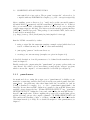
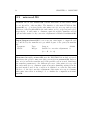
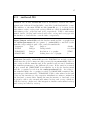
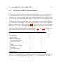
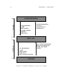
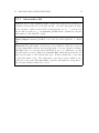
that are exchanged are listed in Table 2.1. The sea ice and ocean model use a
time step of one day. Thus, atmospheric coupling to the sea ice model is performed every 32 time steps, while the sea ice and ocean model are coupled every
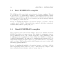
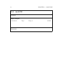
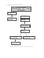
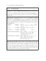
time step. The coupling scheme is shown in Fig. 2.1. Fig. 2.2 shows how the
subroutines are placed when no external coupler is used.
Parameter
Ice cover
Ice thickness
Snow thickness
Surface temperature
Deep sea temperature
Mixed layer depth
Net precipitation, runoff
Salinity
Melt and freeze volume
Heat fluxes
d(Heat fluxes)/dT
Radiation
Wind stress
Atmosphere ← → Ice
←
←
←
←
→
→
→
→
→
Ice ← → Ocean
→
→
←
←
←
→
←
→
→
−
−
→
Table 2.1: Parameters to be exchanged between models. Arrows denote the
direction in which the parameter is passed, e. g. the atmosphere receives ice
cover information from the ice model.
22
CHAPTER 2. MODULES
Timesteps
32
1
Timesteps
1
1
ATMOSPHERE
net precipitation,
runoff,
total heatflux,
sensible heatflux,
radiation,
wind stress
surface temperature,
ice cover,
snow thickness,
ice thickness
SEA ICE
net precipitation,
runoff,
total heatflux,
wind stress,
freeze and melt volume
sea surface temperature,
deep sea temperature,
mixed layer depth,
salinity
OCEAN
Figure 2.1: Schematic illustration of the model coupling.
2.7. SEA ICE AND OCEAN MODULES
23
FLOW DIAGRAM
ATMOSPHERE − ICE − OCEAN
EXCHANGE
PUMA MAIN LOOP
puma.f90
SURFSTEP
surfmod.f90
LANDSTEP
landmod.f90
SEASTEP
seamod.f90
CPLEXCHANGE_ICE
intermod_atm.f90
ICESTEP
icemod.f90
CPLEXCHANGE_OCEAN
iintermod_ice.f90
CPLEXCHANGE_ATMOS
intermod_ice.f90
OCEANSTEP
oceanmod.f90
Figure 2.2: Subroutine flow when no external coupler is used.
24
CHAPTER 2. MODULES
2.7. SEA ICE AND OCEAN MODULES
2.7.1
25
seamod.f90
General The module seamod.f90 deals as an interface between the atmospheric part of the
model and modules for the ocean and sea ice. The basic subroutines seaini, seastep and
seastop are called by the the subroutines surfini, surfstep and surfstop, respectively (see
module surfmod.f90). See the reference guide, section (heiko.coupling) for a visualization
of the module coupling structure.
Input/Output seamod.f90 needs the parameter file surface_parameter to read the
climatological sea surface temperature and ice cover as well as ocean_parameter, which
contains climatological mixed layer depth and the Levitus 400 m temperature. As output
data, the file sea_restart is produced at the end of a run. In the case of a restart, this
file is required to be read in by the module. The namelist seapar, which is contained in
the file sea_namelist, is defined as:
Parameter
Type
Purpose
default
ALBSEA
REAL
Albedo for open water
0.069
ALBICE
REAL
Max. albedo for sea ice
0.7
DZ0SEA
REAL
Roughness length sea
1.5·10−5 m
DZ0ICE
REAL
Roughness length ice
1.0·10−3 m
DRHSSEA
REAL
Wetness factor sea
1.0
DRHSICE
REAL
Wetness factor ice
1.0
NOCEAN
INTEGER Ocean model (1) or cli- 1
matology (0)
NICE
INTEGER Sea ice model (1) or cli- 1
matology (0)
NCPL_ICE_OCEAN INTEGER Ice Ocean coupling time 1
steps
NCPL_ATMOS_ICE INTEGER Atmosphere Ice coupling 32
time steps
SSTFILE
CHAR*80 file containing climatology ”surface_parameter”
Structure Internally, seamod.f90 uses the FORTRAN-90 module seamod, which uses the
global common module pumamod from pumamod.f90. Subroutine seaini reads the namelist
and, if the parallel version is used, distributes the namelist parameters to the different
processes. If the run is not started from a restart file (NRESTART from namelist inp is
0), the sea surface temperature and the ice cover is read from the surface_parameter
file. Ice thickness is computed from ice cover. Additionally, mixed layer depth and the
400 m Levitus temperature is read from the file ocean_parameter. Climatology and
namelist information is passed to the ice and ocean modules via the external subroutines iceini (in icemod.f90) and oceanini (in oceanmod.f90 or oceanmod50.f90). Every
NCPL_ATMOS_ICE time steps, seastep calls the ice module via the external subroutine
cplexchange_ice (defined in intermod_atm.f90). At the end of the integration, seastop
writes the restart information into file sea_restart.
26
2.7.2
CHAPTER 2. MODULES
intermodatm.f90
General The module intermod_atm.f90 contains subroutines that exchange
information between the atmospheric module and the sea ice module. If an
external coupler is used with an independent sea ice / ocean model, the module
is replaced e.g. by mpccimod_atm.f90 which contains the relevant subroutines
for the MpCCI coupler.
Input/Output intermod_atm.f90 does not use any extra input file or output
file.
Structure The subroutines cplstart, cplinit, cplstop are dummy routines that
are real subroutines only in the case of external coupling. The subroutine
cplexchange_ice, which is called by seastep in module seamod.f90, calls the
external subroutine icestep (defined in icemod.f90). It then copies the ice /
ocean data to the relevant PUMA variables.
2.7. SEA ICE AND OCEAN MODULES
2.7.3
27
intermodice.f90
General The module intermod_ice.f90 contains subroutines that exchange information between the sea ice module and the ocean and atmosphere module.
If an external coupler is used with an independent sea ice / ocean model,
the module is replaced e.g. by mpccimod_ice.f90 which contains the relevant
subroutines for the MpCCI coupler.
Input/Output intermod_ice.f90 does not use any extra input file or output
file.
Structure The subroutine cplexchange_ocean, which is called by icestep in
module icemod.f90, calls the external subroutine oceanstep (defined in oceanmod.f90) if the sea_namelist entry NOCEAN is set to 1. Otherwise, it calls
the subroutine oceanget (defined in oceanmod.f90), which interpolates the climatological values to the current time step. It then returns the ocean data
to the subroutine icestep. The subroutine cplexchange_atmos, which is also
called by icestep in module icemod.f90, copies the atmospheric forcing data to
the relevant variables defined in icemod.
28
2.7.4
CHAPTER 2. MODULES
icemod.f90
General The module icemod.f90 contains subroutines to compute sea ice cover
and thickness. The interface to the main PUMA module is given by the subroutine icestep, which is called by cplexchange_ice (defined in intermod_atm.f90),
which is called by seastep (defined in seamod.f90).
Input/Output icemod.f90 requires the file ice_flxcor if NFLXCORR is set to
a negative value. If NOUTPUT is set to 1, the output files fort.75 containing
global fields of ice model data and the file fort.76 containing diagnostic ice
data are produced (for details, see the reference guide). Both output files are
in service format. The module is controlled by the namelist icepar in the file
ice_namelist.
Parameter
Type
Purpose
default
NDIAG
INTEGER Diagnostic output every NDIAG 160
time steps
NOUT
INTEGER Model data output every NOUT 32
time steps
NOUTPUT
INTEGER Icemodel output (0=no,1=yes)
1
NFLXCORR
INTEGER Time constant for restoring (> 0), 360 d
no flux correction (= 0), use fluxcorrection from file (< 0)
Structure icemod.f90 uses the module icemod which is not dependent on
the module pumamod. Subroutine iceini reads the namelist and, when required, the flux correction from the file ice_flxcor. Subroutine icestep calls
cplexchange_atmos (defined in intermod_ice) to get the atmospheric forcing
fields. If the sea_namelist parameter NICE is set to 1, the subroutine subice
is called, which calculates ice cover and thickness. Otherwise, climatological data, interpolated to the current time step by iceget are used. If an ice
cover is present, the surface temperature is calculated in skintemp. Otherwise,
the surface temperature is set to the sea surface temperature calculated by
the ocean model. Every NCPL_ICE_OCEAN (defined in sea_namelist) time
steps, the external subroutine cplexchange_ocean (defined in intermod_ice) is
called to pass the atmospheric forcing to and retrieve oceanic data from the
ocean module oceanmod.f90. The oceanic data is used for ice calculations in
the next time step.
2.7. SEA ICE AND OCEAN MODULES
2.7.5
29
oceanmod.f90
General The module oceanmod.f90 contains a mixed layer ocean model, i.e.
subroutines to compute sea surface temperature and mixed layer depth. The
interface to the main PUMA module is via the module icemod.f90 given by
the subroutine oceanstep, which is called by cplexchange_ocean (defined in
intermod_ice).
Input/Output oceanmod.f90 requires the file ocean_flxcor if NFLXCORRSST or NFLXCORRMLD is set to a negative value. If NOUTPUT
is set to 1, the output file fort.31 containing global fields of ocean model data
in service format is produced (for details, see the ice modul section of the reference guide). The module is controlled by the namelist oceanpar in the file
ocean_namelist.
Parameter
Type
Purpose
default
NDIAG
INTEGER Diagnostic output every NDIAG 480
time steps
NOUT
INTEGER Model data output every NOUT 32
time steps
NOUTPUT
INTEGER Oceanmodel
output 1
(0=no,1=yes)
NFLXCORRMLD INTEGER Time constant for restoring 60 d
mixed layer depth (> 0), no flux
correction (= 0), use fluxcorrection from file (< 0)
NFLXCORRSST INTEGER Time constant for restoring sea 60 d
surface temperature (> 0), no
flux correction (= 0), use fluxcorrection from file (< 0)
Structure oceanmod.f90 uses the module oceanmod which is not dependent
on the module pumamod. Subroutine oceanini reads the namelist and, when
required, the flux corrections from the file ocean_flxcor. Subroutine oceanstep
calls mixocean, which calculates mixed layer depth and temperature. If an ice
cover is present, mixed layer depth is set to the climatological value and the
sea surface temperature is set to the freezing temperature. For details of the
mixed layer model, see the reference guide section (ute).
30
2.7.6
CHAPTER 2. MODULES
oceanmod50.f90
General The module oceanmod50.f90 contains a mixed layer ocean model with
depth fixed to 50 m and a SST fluxcorrection that does not stem from restoring
to climatological data. For details, see section (ute) of the reference guide. The
module oceanmod50.f90 optionally replaces the module oceanmod.f90, so the
internal structure and the interface to the main PUMA module is identical to
oceanmod.f90.
Input/Output If NFLXCORRSST is set to a negative value, oceanmod50.f90
requires the file ocean_lgflxcor (denoting long-term gradient flux correction).
Otherwise, the file heat_parameter is needed to calculate the flux correction.
If NOUTPUT is set to 1, the output file fort.31 containing global fields of
ocean model data in service format is produced (for details, see the ice module
section of the reference guide). The module is controlled by the namelist
oceanpar in the file ocean_namelist.
Parameter
Type
Purpose
default
NDIAG
INTEGER Diagnostic output every NDIAG 480
time steps
NOUT
INTEGER Model data output every NOUT 32
time steps
NOUTPUT
INTEGER Oceanmodel
output 1
(0=no,1=yes)
NFLXCORRSST INTEGER Flag for calculating the flux cor- -1
rection (< 0) or reading the flux
correction from file (> 0)
Structure The internal structure is exactly the same as in oceanmod.f90.
Chapter 3
Running PUMA
3.1
Interactive Console Mode
Puma is started from a console by simply typing
puma.x
The following files have to be present in the same directory:
puma_namelist
land_namelist
sea_namelist
ice_namelist
ocean_namelist
surface_parameter
ocean_parameter
All settings, like length of the integration, special parameterizations etc. are
given in the namelist files. The parameter files contain the climatology. When
the integration is finished successfully, the following files have been created:
puma_output
puma_restart
land_restart
sea_restart
The file puma_output contains the model results and has to be postprocessed
using the pumaburner (cf. Chapter ??). The _restart files contain information
necessary to restart the model run from the end of the current integration.
31
32
3.2
CHAPTER 3. RUNNING PUMA
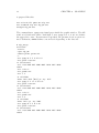
Batch Mode
For long integrations, it is more useful to run puma in batch mode, i.e. start puma
by calling a script that manages the model run. The following script does just
that. Since it is quite long, it is here split to parts with explanations inbetween.
#!/usr/bin/ksh
#
stime=‘date‘
#=========================
# This script runs the atmospheric model PUMA on a linux machine
#
EXP=example
# EXPERIMENT IDENTIFIER
EXPDIR=/castor/home/user/${EXP}
# EXPERIMENT DIRECTORY
MODEL=${EXPDIR}/puma.x
# THE MODEL EXECUTABLE
SCHAUER=1
# TRANSFER OUTPUT TO SCHAUER (1=YES)
SCHAUERDIR=/pf/u/user_account/puma/${EXP} # U-TREE DIRECTORY (FOR OUTPUT)
DATADIR=${EXPDIR}/data
# OUTPUT DIRECTORY
SSTFILE=${EXPDIR}/surface_parameter
# INITIAL DATAFILE (PUMA)
SURFFILE=${EXPDIR}/surface_parameter
# INITIAL DATAFILE (PUMA)
OCEANFILE=${EXPDIR}/ocean_parameter
# INITIAL DATAFILE (OCEANMOD)
LASTYEAR=50
# LAST YEAR TO BE SIMULATED
FTPINT=12
# MONTHS PER TAR-FILE
TMPDIR=${MFHOME}/tmpdir/run$$
#
mkdir -p ${TMPDIR}
cd $TMPDIR
set -ex
mkdir -p ${EXPDIR}
mkdir -p ${DATADIR}
#
OUTYEAR=1
OUTDAY=30
OUTMON=2
OUTFTP=2
TARFILE=${EXP}TAR_0101
#
cp $MODEL $EXPDIR/model.x
#
This first block of the script defines the basic settings, i.e. the directories used,
the length of the integration etc. If SCHAUER is set to 1, all puma output is transferred to the specified directory on the schauer, thus avoiding the users directory
3.2. BATCH MODE
33
from filling up. Otherwise, the output is written to the DATADIR directory. A
temporary directory is created where the model is eventually run.
#
cat > $EXPDIR/NAMLIST.exe << ’EOX’
#
# NAME LIST PARAMETER
#
cat > puma_namelist << EOF
&INP
NDAYS=30,
NTSPD=32,
NRESTART=${1},
NDIAG=480,
NAFTER=32,
NEQSIG=1,
PSURF=101325.,
NPACKSP=0,
NPACKGP=0,
&END
&MISCPAR
&END
&FLUXPAR
&END
&RADPAR
&END
&RAINPAR
&END
&SURFPAR
&END
EOF
#
EOX
#
cat > ${EXPDIR}/land_namelist << EOL
&landpar
&end
EOL
cat > ${EXPDIR}/sea_namelist << EOO
&seapar
&end
EOO
cat > ${EXPDIR}/ocean_namelist << EOO
34
CHAPTER 3. RUNNING PUMA
&oceanpar
&end
EOO
cat > ${EXPDIR}/ice_namelist << EOO
&icepar
&end
EOO
#
chmod u+x ${EXPDIR}/NAMLIST.exe
#
Now, the necessary namelists are generated. The puma namelist is defined as an
executable which can be called with a parameter setting the restart mode.
$EXPDIR/NAMLIST.exe 0
cp ${EXPDIR}/land_namelist land_namelist
cp ${EXPDIR}/sea_namelist sea_namelist
cp ${EXPDIR}/ice_namelist ice_namelist
cp ${EXPDIR}/ocean_namelist ocean_namelist
#
cp $EXPDIR/model.x model.x
cp ${SSTFILE} surface_parameter
cp ${SURFFILE} surface_parameter
cp ${OCEANFILE} ocean_parameter
#
model.x > ${EXPDIR}/${EXP}PROUT_0101
#
mv puma_output ${EXP}PUMA_0101
#
# history and restart saved for further diagnostics
#
tar -cf ${EXPDIR}/${TARFILE} ${EXP}PUMA_0101
mv puma_restart $EXPDIR/${EXP}RES
mv land_restart $EXPDIR/${EXP}LANDRES
mv sea_restart $EXPDIR/${EXP}SEARES
#
echo ${OUTYEAR} > ${EXPDIR}/saveyear.${EXP}
echo ${OUTDAY} > ${EXPDIR}/saveday.${EXP}
echo ${OUTMON} > ${EXPDIR}/savemon.${EXP}
echo ${OUTFTP} > ${EXPDIR}/saveftp.${EXP}
echo ${TARFILE} > ${EXPDIR}/savetar.${EXP}
#
3.2. BATCH MODE
35
# cat runall to EXPDIR
#
cat > $EXPDIR/runall << EOR
#!/usr/bin/ksh
#
TMPDIR=${TMPDIR}
mkdir -p \${TMPDIR}
cd \$TMPDIR
set -ex
#
EXPDIR=$EXPDIR
SCHAUER=$SCHAUER
SCHAUERDIR=$SCHAUERDIR
DATADIR=$DATADIR
EXP=$EXP
LASTYEAR=$LASTYEAR
MONTHS=$MONTHS
FTPINT=$FTPINT
The puma namelist is generated with NRESTART=0, i.e. the first month is integrated from climatology. The script runall is generated, which can be used to
restart the run after an interruption.
The remainder of the script is a loop of one-month integrations until the desired integration time is reached. After each year, the monthly output is tarred
together and moved to the schauer or the data directory.
#
cp \${EXPDIR}/model.x model.x
#
##################################################################
#
II=1
while [ \$II -le 2 ]
do
#
INMON=\‘cat \${EXPDIR}/savemon.\${EXP}\‘
INYEAR=\‘cat \${EXPDIR}/saveyear.\${EXP}\‘
INDAY=\‘cat \${EXPDIR}/saveday.\${EXP}\‘
INFTP=\‘cat \${EXPDIR}/saveftp.\${EXP}\‘
TARFILE=\‘cat \${EXPDIR}/savetar.\${EXP}\‘
#
YY=\$INYEAR
36
CHAPTER 3. RUNNING PUMA
if [ \${INYEAR} -lt 10 ]
then
YY=0\${YY}
fi
MM=\$INMON
if [ \${INMON} -lt 10 ]
then
MM=0\${MM}
fi
#
# make namelist
#
\$EXPDIR/NAMLIST.exe 1
cp \${EXPDIR}/land_namelist land_namelist
cp \${EXPDIR}/sea_namelist sea_namelist
cp \${EXPDIR}/ice_namelist ice_namelist
cp \${EXPDIR}/ocean_namelist ocean_namelist
#
cp \$EXPDIR/\${EXP}RES puma_restart
cp \$EXPDIR/\${EXP}LANDRES land_restart
cp \$EXPDIR/\${EXP}SEARES sea_restart
#
model.x > \${EXPDIR}/\${EXP}PROUT_\${YY}\${MM}
#
# history and restart saved for further diagnostics
#
mv puma_output \${EXP}PUMA_\${YY}\${MM}
#
if [ \${INFTP} -eq 1 ]
then
TARFILE=\${EXP}TAR_\${YY}\${MM}
echo \${TARFILE} > \${EXPDIR}/savetar.\${EXP}
tar -cf \${EXPDIR}/\${TARFILE} \${EXP}PUMA_\${YY}\${MM}
else
tar -rf \${EXPDIR}/\${TARFILE} \${EXP}PUMA_\${YY}\${MM}
fi
mv puma_restart \$EXPDIR/\${EXP}RES
mv land_restart \$EXPDIR/\${EXP}LANDRES
mv sea_restart \$EXPDIR/\${EXP}SEARES
rm \${EXP}PUMA_\${YY}\${MM}
#
OUTMON=\‘expr \${INMON} + 1\‘
OUTDAY=\‘expr \${INDAY} + 30\‘
3.2. BATCH MODE
37
OUTYEAR=\${INYEAR}
OUTFTP=\‘expr \${INFTP} + 1\‘
#
if [ \${OUTMON} -eq 13 ]
then
OUTMON=1
OUTYEAR=\‘expr \${OUTYEAR} + 1\‘
fi
#
echo \${OUTYEAR} > \${EXPDIR}/saveyear.\${EXP}
echo \${OUTMON} > \${EXPDIR}/savemon.\${EXP}
echo \${OUTDAY} > \${EXPDIR}/saveday.\${EXP}
#
################################################################
#
if [ \${OUTFTP} -gt \${FTPINT} ]
then
#
cd \${EXPDIR}
OUTFTP=1
echo \${OUTFTP} > \${EXPDIR}/saveftp.\${EXP}
tar -rf \${EXPDIR}/\${TARFILE} \${EXP}RES
tar -rf \${EXPDIR}/\${TARFILE} \${EXP}LANDRES
tar -rf \${EXPDIR}/\${TARFILE} \${EXP}SEARES
tar -rf \${EXPDIR}/\${TARFILE} NAMLIST.exe
tar -rf \${EXPDIR}/\${TARFILE} land_namelist
tar -rf \${EXPDIR}/\${TARFILE} sea_namelist
tar -rf \${EXPDIR}/\${TARFILE} ice_namelist
tar -rf \${EXPDIR}/\${TARFILE} ocean_namelist
tar -rf \${EXPDIR}/\${TARFILE} saveday.\${EXP}
tar -rf \${EXPDIR}/\${TARFILE} savemon.\${EXP}
tar -rf \${EXPDIR}/\${TARFILE} saveyear.\${EXP}
tar -rf \${EXPDIR}/\${TARFILE} savetar.\${EXP}
tar -rf \${EXPDIR}/\${TARFILE} saveftp.\${EXP}
tar -rf \${EXPDIR}/\${TARFILE} model.x
tar -rf \${EXPDIR}/\${TARFILE} runall
mv \${EXPDIR}/\${TARFILE} \${DATADIR}/\${TARFILE}to\${YY}\${MM}
if [ \${SCHAUER} -eq 1 ]
then
cat > \${EXPDIR}/put_schauer\${YY}\${MM} << EOP
set -ex
cd \${EXPDIR}
/home/larry/utils/uput2 \${DATADIR}/\${TARFILE}to\${YY}\${MM} \${SCHAUERDIR}/\${TAR
38
CHAPTER 3. RUNNING PUMA
rm \${DATADIR}/\${TARFILE}to\${YY}\${MM}
EOP
chmod u+x \${EXPDIR}/put_schauer\${YY}\${MM}
\${EXPDIR}/put_schauer\${YY}\${MM} > \${EXPDIR}/put_\${YY}\${MM} 2>&1 &
fi
cd \$TMPDIR
fi
#
echo \${OUTFTP} > \${EXPDIR}/saveftp.\${EXP}
#
if [ \${OUTYEAR} -gt \${LASTYEAR} ]
then
cd \${EXPDIR}
rm -r \${TMPDIR}
exit
fi
#
exit
EOR
#
cd $EXPDIR
chmod u+x runall
runall
#
etime=‘date‘
echo " "
echo "==> started, $stime"
echo " "
echo "==> done,
$etime"
echo " "
#
exit
Chapter 4
Graphical User Interface
4.0.1
Introduction
The Graphical User Interface (GUI) for the Planet Simulator provides the user
with an interactive mode designed to aid in tuning of parameterization and debugging of the PUMA simulation program.
The configuration of different experiments is handled easily by the structured
graphical input of all model parameters (predefined for unexperienced users),
those who remain static during a run as well as the user defined interactive
parameters who are selected and changed at any time with direct effect on the
running model.
An online visualisation of climate variables as they are computed may be displayed during the run, the visualisation parameters may also be adapted during
the run.
The GUI supports the control of different versions of the simulation program with
different configurations, which can run also remotely on another machine than
the graphical tool.
4.0.2
Installing the PlaisirGUI
This chapter describes the installation of the GUI. The installation of the GUI
and the GUI itself were so far tested only under SuSE Linux and this installation
is written for an Linux installation.
Installation and use of the GUI require the following software:
• Perl 5.6,
39
40
CHAPTER 4. GRAPHICAL USER INTERFACE
• Java RE 1.4.0 (we recommend Java RE 1.4.2) and
• GrADS 1.8
Perl 5.6 is installed directly by most Linux distributions in the developer packages. Furthermore installation software for Perl is found in the web at CPAN1 or
ActiveState2 . If needed, JRE (Java Runtime Enviroment) software can be downloaded from Blackdown3 or SUN4 and GrADS is to be obtained on the GrADS
home page5 .
The installation archive of the GUI is named PlaisirGUI-1.0-install.tar.gz
for the version 1.0.
For installation the archive must be unpacked to an arbitrary directory:
gunzip PlaisirGUI-1.0-install.tar.gz
# uncompress the archive
tar xf PlaisirGUI-1.0-install.tar
# unpack it
tar xzf PlaisirGUI-1.0-install.tar
# uncompress and
or
# unpack the archive
if GNU tar is used.
After that the installation script must be started:
cd PlaisirGUI-1.0
perl setup
or simply
./setup
if Perl is located in /usr/bin.
At the beginning of the installation the script asks for the binary paths of Java2,
Perl and GrADS and the library paths of GrADS, respectivly, as well as for the
destination path of the installation. The default paths and the names of the
corresponding enviroment variables for the directories are:
1
• Java2 binary:
/usr/lib/java/bin
JAVA BIN
• Perl binary:
/usr/bin
PERL BIN
• GrADS binary:
/usr/local/grads/bin
GRADS BIN
• target directory:
~ /PlaisirGUI
http://www.cpan.org/
http://www.activestate.com/
3
http://www.blackdown.org/
4
http://java.sun.com/
5
http://grads.iges.org/grads/
2
41
To accept a default path the input can be confirmed with <RETURN>. For the
directories also relative paths are allowed. When you already entered all paths
you can correct individual directories or confirm the installation.
To use GrADS, in addition to the binary path two more environment variables
have to be set. If these variables are not found by the installation script, the path
names will be queried. These two variables are listed in the following, the given
path names are the standard paths which are used also in the installation script:
• GrADS font files:
/usr/local/grads/dat
GADDIR
• GrADS library:
/usr/local/grads/lib
GASCRP
After completion of the installation script you can change the working directory
to the PlaisirGUI directory, and the GUI can be started:
cd ~ /PlaisirGUI
bin/plaisirgui
Alternativly you can put the binary directory to the standard path variable PATH.
E.g. (bash): export PATH=<gui home dir>/bin:$PATH. Afterwards you can
start the GUI program with plaisirgui from wherever you want, e.g. the working directory.
If you want to reconfigure some binary or library paths for tests or permanently
you can reset the following enviroment variables: JAVA BIN, PERL BIN, GRADS BIN,
GADDIR and GASCRP.
The installation script creates five new subdirectories in the target directory. The
directory bin contains a link to a Perl script starting the GUI.
The directory examples contains some example files. If you choose a different
working directory as our run example, remember to copy the contents of the
example/run directory into your favorite working directory. Otherwise it is possible, that PUMA stops running.
In the directory lib the necessary Java byte code files are located. The directory
scripts contains the Perl scripts of the program.
The standard output and the error messages of the simulation program (e.g.
PUMA) and of GrADS will be written into log files. Normally there are three
log files in the directory where you start the GUI:
42
CHAPTER 4. GRAPHICAL USER INTERFACE
• plaisirgui.log
• plaisirgui.grads.log
• plaisirgui.puma.log
The first log file includes the logging data from the GUI program, the second file
includes the logging of GrADS and the third one of PUMA. If the logging was
not deleted before starting the GUI, the old log, created on the last running day,
the files will be renamed by adding the date to the file extension and the new
logging will be written into the known files.
You will find more about logging in section 4.0.3.3.3, Logging Menu, and in
section 4.0.4, Troubleshooting.
4.0.3
Operating
4.0.3.1
Starting and Terminating
The GUI is started with
bin/plaisirgui
in case you are in the PlaisirGUI main directory, or with
plaisirgui
if the bin directory is located in the standard path.
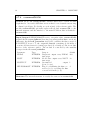
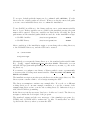
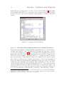
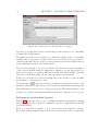
Then the main window of the GUI appears (figure 4.1. PlaisirGUI can be terminated either by the menu option File → Exit Program or by the close icon of the
main window border.
4.0.3.2
Adjusting the Simulation Program and the Working Directory
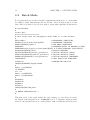
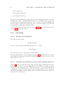
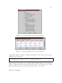
Figure 4.2 shows the GUI file menu with six menu entries. With the first three
menu items you can choose the working directory, the PUMA executable program,
and the model configuration file. With the next two you can save the model
configuration. And the last file menu item closes the GUI program, terminates
the PUMA simulation if still running and the GrADS windows, and saves the
actual model configuration.
43
Figure 4.1: PlaisirGUI Main Window
Selecting the simulation program and the working directory
It is possible to select the working directory under File → Select working directory.
All input data have to be located there (e.g. surface parameter), and all output
data will be put there. The first time the GUI is started, the working directory is
set to the starting directory, when the program is restarted the working directory
is set to the last used path.
With the menu item File → Select simulation executable the simulation program
can be adjusted for the next run. It will be inquired whether the model configuration file is to be used, whose name is derived from the program (i.e. program.cfg). Alternatively the pre-selected configuration will be kept in use.
Loading and Saving model configuration
Under File → Load model configuration file a model configuration is specified,
which contains the initialisation of all modelling parameters (see part II, sec-
44
CHAPTER 4. GRAPHICAL USER INTERFACE
tion ??). It is necessary to configure the model before choosing or modifying the
static and interactive modelling parameters (see section 4.0.3.3).
Figure 4.2: File Menu
The next file menu items save the current model . The simple File→Save model
configuration file item overwrites the old configuration. In the item File→Save
model configuration file as you can save the configuration in a different file as
derived from the previous configuration.
4.0.3.3
Setting Optional Parameters
The substantial component in the GUI concept are the model parameters, which
are defined in the model configuration file and which are provided for PUMA
by the Fortran namelists (see part II, section ??). There are two categories
of parameters. On the one hand there are static ones, which remain constant
during a run, and on the other hand we have parameters that can be interactively
changed during the run. Before starting a simulation run therefore different
settings have to be made:
• check-up or redefinition of the static parameters
• selection of the interactive parameters
• specification of the interactive parameters
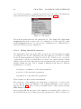
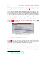
These settings are made in the menu Options.
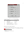
The execution of the simulation program may be redirected to a remote host
by choosing the menu item Options → Set Program Parameters. A new window
appears (see fig. 4.4), where a remote hostname may be entered after selecting
Make Remote Connection.
After pressing OK the next run of the simulation executable will be started on
the specified remote host, Cancel rejects this specification). This is realized by a
45
Figure 4.3: Options Menu
Unix remote shell (command rsh, so for the successful start the working directory
must be remotely mounted, the user credentials must be set and the .rhosts file
must have an entry for the machine where the GUI is running. 6
Figure 4.4: Program Parameters
4.0.3.3.1
Setting the Initial Model Parameters
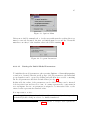
To initialize the model parameters, after pressing Options → Set model properties,
a window is obtained, that shows all groups of model parameters; the individual
group branches can be opened by clicking and will then show a table containing
the model parameters and their default values (see fig. 4.5).
In this table the values of the parameters can be edited. Values can be inserted
both in scalar form and in vector form. A comma separates the components in
vectorial inputs. In case one parameter is assigned to be interactive later on, the
entered value represents its standard value.
It is important to notice:
Any changes have to be confirmed either with <RETURN> or by selecting another
form field (double click), in order to be finally transferred.
6
The simulation executable (see section 4.0.3.2) may also be a script to start a parallel run.
46
CHAPTER 4. GRAPHICAL USER INTERFACE
With OK these settings will be accepted for the next PUMA run7 , with Reset
the standard values will be recovered and can be changed again, whereas Cancel
leads to rejection of the selected attitudes. Subsequently, you return to the main
window.
Figure 4.5: Setting Model Parameters
4.0.3.3.2
Selecting and Configuring Interactive Model Parameters
The menu entry Options → Select interactive parameters made for the interactive
PUMA control leads to a list of parameters, from which the interactive ones can
be selected by clicking (see fig 4.6). Up to four interactive parameters are allowed.
Reset deletes the whole choice and new parameters can be selected. Cancel rejects
the selection and returns to the main window, to continue execution with the
previous parameters. With OK the selection is confirmed and a window with a
table appears, which serves for further specification of the selected parameters.
Beside the name the standard value (initialized by the table value of the static
parameters), the minimum and maximum values (initialized by 90% and 110%
of the standard value), the increment (initialized as 1% of the standard value)
and the maximum change per time step Delta (that so far always is equal to the
increment) are denoted. Any data except the name are changeable, whereby it
is to be noted that the conditions Min ≤ Default ≤ Max and Step ≤ Delta ≤
7
The PUMA namelist parameter nrun or ndays must either be the total amount of simulation
time steps or days to simulate or has to be set to negative. The last case causes an infinite
simulation loop until it is ended by the GUI’s control panel.
47
Figure 4.6: Selecting Interactive Model Parameters
Figure 4.7: Specifying Interactive Model Parameters
(Max−Min) must be satisfied. Further plausibility checks will be made by the
simulation program itself.
Any changes have to be confirmed either with <RETURN> or by selecting another
form field (double click), in order to be finally transferred.
Reset changes any values to the default values, Back returns to the selection
window. Cancel neglects all changes and leads back to the main window. With
OK the defined values are saved and the main window is reopened.
4.0.3.3.3
Logging
48
CHAPTER 4. GRAPHICAL USER INTERFACE
The GUI program logs all standard and error output to the starting console and
to a log file. For logging the logging framework log4j 8 by the Jakarta Apache
Project is used.
The logging menu Options→Logging Parameters includes three entries in a submenu. The first item in this submenu, Logging Parameters→Log-Window, opens
a logging window from log4j. The logging configuration is changed automatically
to verbose logging when opening the logging window. The second entry is a menu
checkbox called Logging Parameters→Advanced Logging. This checkbox activates
only a verbose logging, there will be no logging window opened. The last menu
entry is Logging Parameters→Clear Logs and deletes all logging data in the actual
log files.
In section 4.0.4, Troubleshooting, and the Programmers Guide, part II, ??
are more details about logging.
Figure 4.8: Entries in Logging Menu
4.0.3.4
Running the Simulation Program
Figure 4.9 shows the control panel together with three GrADS frames which
display the actual state of temperature and wind force. The control panel is
divided into three parts: Interactive, Visualisation and Simulation.
With the displayed sliders in the first part of the main window, model parameters can be changed interactively during the simulation. In order to pass these
adjustments on to the simulation, the running program must be interrupted and
the button Set of the section Interactive has to be pushed. When the simulation
program has accepted the new parameters, the calculations can be continued.
The button Reset puts all parameters to the initial values. After pressing the
button Set the old setting is lost.
8
log4j: http://jakarta/apache.org/log4j
49
Figure 4.9: Control Panel
50
CHAPTER 4. GRAPHICAL USER INTERFACE
The second part of the window shows the check boxes for the interactive visualisation of simulation results. Up to four variables can be selected before and
during the simulation. The graphical display of simulation results starts as soon
as the simulation is running.
There are three buttons on the right side of the visulisation panel. The first
button opens a dialogbox to edit the visualisation parameters, which is described
below. The middle button opens all GrADS windows and the last button closes
all open GrADS applications.
The third sector serves for the control of the simulation, where the symbols stand
for the following:
starting / continuing the simulation
interrupting the simulation
terminating the simulation
The START button ( ) starts the simulation. If variables were already activated
for displaying results before the start, they are shown now in separate windows.
To interrupt the simulation only for a short interruption, PAUSE ( ) is pushed.
The latest shown visualisation windows remain visible. To continue the simulation the START button has to be pushed again.
The third button ( ) serves for stopping the running simulation. The lastly shown
graphics remain visible. At the bottom of the simulation panel is a progressbar
which shows the actual step of the simulation. If the namelist parameter nrun
resp. ndays is set to be negative, which means that the running simulation is set
to infinite loop, the progressbar will restart on each 1000th step. This increment
can be changed with model parameter progressbar, see section ??, part II.
4.0.3.4.1
Configuring the Visualisation
The gui allows to visualise actually generated simulation output. The file format
used for the interim output is NetCDF format, which can be read and displayed
with GrADS.
It is possible to reconfigure the visualisation properties without any handling in
the property files. To configure the visualisation it is neccessary to know which
data variables the simulation writes into the NetCDF files. For the delivered simulation program, <gui home dir>/example/run/puma scalar static.x, there
are seven variables in the NetCDF output:
51
Figure 4.10: Visualisation Dialogbox
Variable
Description
Free coordinates
p0
dt
t
u
du
v
dv
Surface pressure
Temperature
Temperature11
Zonal wind component11
Zonal wind component
Meridional wind component11
Meridional wind component
lon9 , lat10
lon, lat, lev
lat, lev12
lat, lev
lon, lat, lev
lat, lev
lon, lat, lev
Dialogbox for the Common properties
To configure the GrADS output the GUI includes a dialogbox, which can be
opened with the button Edit Visu Parameter ... in the Visualisation panel. Figure
4.10 shows this dialog box.
9
longitude
latitude
11
cross section along the Greenwich meridian
12
atmospheric level
10
52
CHAPTER 4. GRAPHICAL USER INTERFACE
Figure 4.11: Dialog Box for the Detailed Properties
The dialogbox panel shows four rows with buttons and checkboxes etc. and finally
a Cancel and an OK button.
The first item in the row is a checkbox to enable the editing of the corresponding
GrADS window properties. If this checkbox is not selected it is not possible to
edit this item in the dialogbox and you can’t start the associated GrADS windows
in the visualisation panel of the main window.
The second item in the row is a pop down list. The list title is a short description
of the selected GrADS window configuration. In this pop down list another box
item can be selected to display different NetCDF data with GrADS. Selecting
another box item will change all associated properties automatically.
If the second checkbox is selected GrADS shows the deviation of the monthly
mean values to saved reference data.
The next button
opens a new dialogbox with more detailed properties of the
GrADS configuration. This dialogbox is described in detail in the next paragraph.
If the OK button on the bottom of the panel is pressed the actual changes of the
settings are accepted and with the Cancel button these changes can be rejected.
Dialogbox for the Detailed Properties
Figure 4.11 shows the dialog box to configure visualisation parameters. In this
dialogbox there are more detailed configurable options for displaying the NetCDF
data with GrADS.
Each pop down list is editable, so you can add any new element to the list.
Removing with the Remove button deletes the actual item of the corresponding
53
pop down list in the row and replaces this item with the last element in the list.
With the pop down list you can change the actual entry by any other item in the
list.
Rembember when changing anything in this dialogbox, the box doesn’t check any
coherency with other items in the dialogbox.
This warning means for example if you change the title entry from temperature
to pressure the dialogbox won’t change anything else in the other rows, neither
the short title nor the formula or anything sensible else.
In the following table you find an overview about the seven elements of the
dialogbox and some input examples:
Label
Title
Short Title
Formula
Level
Longitude
Latitude
Color Level
Description
Full title, displayed in the GrADS window
Short title, displayed in the visualisation panel
of the main window
With this formula GrADS displays the NetCDF data,
e.g. dt-273.15 or du;dv;hcurl(du,dv)
Atmospheric pressure level(s)
e.g. 0, 1000 or 0 1000
Global longitudes
e.g. 0 or 0 360
Global latitudes
e.g. 0 or -90 90
Level range of colors which GrADS will use
e.g. -40 -35 -30 -25 -20 -15 -10 -5 0 5 10 15 20
In the list for level, longitude and latitude may only be entries with one or two
numbers. The third examples for the formula is more complex than the others:
du;dv;hcurl(du,dv). The semicolon divides the variables. The list for the color
levels may include one or more numbers. If the input for level, longitude and
latitude includes more than one number, the numbers are divided with space.
There is a special addon to display the wind vectors. There has to be the keyword
wind in the title string of the displayed GrADS window and the formula mag(u,v)
must be used.
4.0.3.5
Changing the environment
4.0.4
Trouble Shooting
This section provides answers to frequently asked questions about the GUI.
54
CHAPTER 4. GRAPHICAL USER INTERFACE
4.0.4.1
Where are the logfiles?
4.0.5
Additional Tools
For demonstration purposes, data snapshots of a special PUMA run can be saved
to show them later as a movie which the GUI can display. The look and feel of the
visualized data is the same as that of a concrete PUMA run. The snapshots are
also the basis to create a reference file used to compute and visualise deviations
to the actually computed data by PUMA.
Depending on the value of writeStep (default: 32, set in the GUI namelist, see
part II, section ??), an output of the actual values of some PUMA variables will
be written into the snapshot netCDF file puma var.nc. Additionally after each
month, the mean values over all written values for the preceeding month are
written into the netCDF file puma mean.nc. These files are read permanently by
the visualisation part of the GUI.
4.0.5.1
Running a Movie
If the parameter makemovie (default: false, set in the GUI namelist, see part
II, section ??) is set to true, a copy of each newly written file puma var.nc
and puma mean.nc is stored in the directory pumamovie, which will be created if necessary. These copies will have the filenames puma var.nc 000000 and
puma mean.nc 000000, where 000000 is replaced by the actual timestep. The
names of the files are saved in the files puma var.dat and puma mean.dat, for use
in the puma movie tool.
For using this tool, it is necessary to set the simulation executable (File → Select simulation executable) to the examples/exec/puma movie.x program. The
working directory (File → Select working directory) must be set to the directory
with the formerly created movie files (if not changed, this is pumamovie). When
starting the program, puma movie offers the movie files one after the other for
visualisation.
The model configuration file (see part II, section ?? ) may include a special group
movie described by the entries
&movie movie_namelist movie parameters
waitTime
3
1000.0 false
wait x msec per time step
The waitTime Parameter tells the movie program the number of microseconds
to wait before changing to the next snapshot. The other entries in the model
55
configuration file have no effect on the movie run, except for the progressBar
entry in the gui group, which is recommended to be changed to a suitable value
for the movie run (default: 200 msec). The value should leave the viewer enough
time to look at each displayed graphic.
4.0.5.2
Creating a Reference
Movie data can also be used to create a reference file by the puma reference
tool. The program examples/exec/puma reference.x converts a number of input
files like puma var.nc into a file puma reference.nc containing the monthly means
for one year of data. The number of input files must be dividable by 12. The
provided file examples/ref/puma reference.nc contains the monthly means of the
third year of a PUMA run based on the provided model configuration file.
The current version of the puma reference tool has to be adapted if the variables
written to puma var.nc change.
56
CHAPTER 4. GRAPHICAL USER INTERFACE
Chapter 5
Postprocessing
5.1
Pumaburner
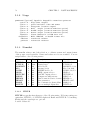
5.1.1
Introduction
The Pumaburner is a postprocessor for the Planet Simulator and the PUMA
model family. It’s the only interface between raw model data output and diagnostics, graphics, and user software.
The output data of the Planet Simulator are stored as packed binary (16 bit)
values using the model representation. Prognostic variables like temperature,
divergence, vorticity, pressure, and humidity are stored as coefficients of spherical
harmonics on σ levels. Variables like radiation, precipitation, evaporation, clouds,
and other fields of the parameterization package are stored on Gaussian grids.
The tasks of the Pumaburner are:
• Unpack the raw data to full real representation.
• Transform variables from the model’s representation to a user selectable
format, e.g. grids, zonal mean cross sections, fourier coefficients.
• Calculate diagnostic variables, like vertical velocity, geopotential height,
wind components, etc.
• Transfrom variables from σ levels to user selectable pressure levels.
• Compute monthly means and standard deviations.
• Write selected data either in SERVICE, GRIB, or NetCDF format for further processing.
57
58
5.1.2
CHAPTER 5. POSTPROCESSING
Usage
pumaburn4 [options] InputFile OutputFile <namelist >printout
option -h : help (this output)
option -c : print available codes and names
option -d : debug mode (verbose output)
option -g : Grib
output (override namelist option)
option -n : NetCDF output (override namelist option)
option -m : Mean=1 output (override namelist option)
InputFile : Planet Simulator or PUMA data file
OutputFile : GRIB, SERVICE, or NetCDF format file
namelist : redirected <stdin>
printout : redirected <stdout>
5.1.3
Namelist
The namelist values control the selection, coordinate system and output format
of the postprocessed variables. Names and values are not case sensitive. You can
assign values to the following names:
Name
Def.
HTYPE
S
VTYPE
S
MODLEV
0
hPa
0
CODE
0
GRIB
0
NETCDF
0
MEAN
1
HHMM
1
HEAD7
0
MARS
0
MULTI
0
5.1.3.1
Type
char
char
int
real
int
int
int
int
int
int
int
int
Description
Horizontal type
Vertical type
Model levels
Pressure levels
ECMWF field code
GRIB output selector
NetCDF output selector
Compute monthly means
Time format in Service format
User parameter
Use constants for planet Mars
Process multiple input files
Example
HTYPE=G
VTYPE=P
MODLEV=2,3,4
hPa=500,1000
CODE=130,152
GRIB=1
NETCDF=1
MEAN=0
HHMM=0
HEAD7=0815
MARS=1
MULTI=12
HTYPE
HTYPE accepts the first character of the following string. Following settings are
equivalent: HTYPE = S, HTYPE=Spherical Harmonics HTYPE = Something.
Blanks and the equal-sign are optional.
Possible Values are:
5.1. PUMABURNER
Setting
HTYPE
HTYPE
HTYPE
HTYPE
5.1.3.2
=
=
=
=
S
F
Z
G
Description
Spherical Harmonics
Fourier Coefficients
Zonal Means
Gauss Grid
59
Dimension for T21 resolution
(506):(22 * 23 coefficients)
(32,42):(latitudes,wavenumber)
(32,levels):(latitudes,levels)
(64,32):(longitudes,latitudes)
VTYPE
VTYPE accepts the first character of the following string. Following settings
are equivalent: VTYPE = S, VTYPE=Sigma VTYPE = Super. Blanks and the
equal-sign are optional.
Possible Values are:
Setting
VTYPE = S
VTYPE = P
5.1.3.3
Description
Sigma (model) levels
Pressure levels
Remark
Some derived variables are not available
Interpolation to pressure levels
MODLEV
MODLEV is used in combination with VTYPE = S. If VTYPE is not set to
Sigma, the contents of MODLEV are ignored. MODLEV is an integer array that
can get as many values as there are levels in the model output. The levels are
numbered from top of the atmosphere to the bottom. The number of levels and
the corresponding sigma values are listed in the pumaburner printout. The outputfile orders the level according to the MODLEV values. MODLEV=1,2,3,4,5
produces an output file of five model levels sorted from top to bottom, while
MODLEV=5,4,3,2,1 sorts them from bottom to top.
5.1.3.4
hPa
hPa is used in combination with VTYPE = P. If VTYPE is not set to Pressure, the contents of hPa are ignored. hPa is a real array that accepts pressure
values with the units hectoPascal or millibar. All output variables will be interpolated to the selected pressure levels. There is no extrapolation on the top of
the atmosphere. For pressure values, that are lower than that of the model’s top
level, the top level value of the variable is taken. The variables temperature and
geopotential height are extrapolated if the selected pressure is higher than the
surface pressure. All other variables are set to the value of the lowest mode level
for this case. The outputfile contains the levels in the same order as set in hPa.
Example: hpa = 100,300,500,700,850,900,1000.
60
CHAPTER 5. POSTPROCESSING
5.1.3.5
MEAN
MEAN can be used to compute montly means and/or deviations. The Pumaburner reads date and time information from the model file and handles different
lengths of months and output intervals correctly.
Setting
Description
MEAN = 0 Do no averaging - all terms are processed.
MEAN = 1 Compute and write monthly mean fields. Not for spherical harmonics, Fourier coefficients or zonal means on sigma levels.
MEAN = 2 Compute and write monthly deviations. Not for spherical harmonics, Fourier coefficients or zonal means on sigma levels. Deviations
are not available for NetCDF output.
MEAN = 3 Combination of MEAN=1 and MEAN=2. Each mean field is followed by a deviation field with an identical header record. Not for
spherical harmonics, Fourier coefficients or zonal means on sigma
levels.
5.1.4
Format of output data
The pumaburner supports three different output formats:
• GRIB (GRIdded Binary) WMO standard for gridded data.
• NetCDF (Network Common Data Format)
• Service Format for user readable data (see below).
For more detailed descriptions see for example:
http://www.nws.noaa.gov/om/ord/iob/NOAAPORT/resources/
Setting
Description
GRIB = 1 NetCDF = 0 The output file is written GRIB format. This option
can be used only for HTYPE=Spherical Harmonics or
HTYPE=Gauss Grid.
GRIB = 0 NetCDF = 1 The output file is written in NetCDF format. This option can be used for HTYPE=Gauss Grid only.
GRIB = 0 NetCDF = 0 The output file is written in Service format. This is
the preferred format for user programs. For a detailed
description see the following section.
GRIB = 1 NetCDF = 1 Illegal combination.
5.1. PUMABURNER
5.1.5
61
SERVICE format
The SERVICE format uses the following structure: The whole file consists of
pairs of header records and data records. The header record is an integer array
of 8 elements.
head(1)
head(2)
head(3)
head(4)
head(5)
head(6)
head(7)
head(8)
=
=
=
=
=
=
=
=
ECMWF field code
modellevel or pressure in [Pa]
date [yymmdd] (yymm00 for monthly means)
time [hhmm] or [hh] for HHMM=0
1. dimension of data array
2. dimension of data array
may be set with the parameter HEAD7
experiment number (extracted from filename)
Example for reading the SERVICE format (GRIB=0 , NETCDF=0)
INTEGER HEAD(8)
REAL
FIELD(64,32)
! dimensions for T21 grids
READ (10,ERR=888,END=999) HEAD
READ (10,ERR=888,END=999) FIELD
....
888 STOP ’I/O ERR’
999 STOP ’EOF’
....
5.1.6
HHMM
Setting
Description
HHMM = 0 head(4) shows the time in hours (HH).
HHMM = 1 head(4) shows the time in hours and minutes (HHMM).
5.1.7
HEAD7
The 7th. element of the header is reserved for the user. It may be used for
experiment numbers, flags or anything else. Setting HEAD7 to a number exports
this number to every header record in the output file (SERVICE format only).
62
CHAPTER 5. POSTPROCESSING
5.1.8
MARS
This parameter is used for processing simulations of the Mars atmosphere. Setting
MARS=1 switches gravity, gas constant and planet radius to the correct values
for the planet Mars.
5.1.9
MULTI
The parameter MULTI can bes used to process a series of input data within one
run of the pumaburner. Setting MULTI to a number (n) tells the pumaburner to
procees (n) input files. The input files must follow one of the following two rules:
• YYMM rule: The last four characters of the filename contain the data in
the form YYMM.
• .NNN rule: The last four characters of the filename consist of a dot followed
ny a 3-digit sequence number.
Examples:
Namelist contains MULTI=3
Command: pumaburn <namelist >printout run.005 out
pumaburn processes the files <run.005> <run.006> <run.007>
Namelist contains MULTI=4
Command: pumaburn <namelist >printout exp0211 out
pumaburn processes the files <exp0211> <exp0212> <exp0301> <exp0302>
5.1.10
Namelist example
VTYPE
HTYPE
CODE
hPa
MEAN
GRIB
NETCDF
=
=
=
=
=
=
=
Pressure
Grid
130,131,132
200,500,700,850,1000
0
0
0
This namelist will write Temperature(130), u(130) and v(131) on pressure levels
200hPa, 500hPa, 700hPa, 850hPa and 1000hPa. The output interval is the same
as found on the model data, e.g. every 12 or every 6 hours (MEAN=0). The
output format is SERVICE format.
5.1. PUMABURNER
5.1.11
63
Troubleshooting
If the pumaburner reports an error or doesn’t produce the expected results, try
the following:
• Check your namelist, especially for invalid codes, types and levels.
• Run the pumaburner in debug-mode by using the option -d. Example:
pumaburn <namelist >printout -d data.in data.out
This will print out some details like parameters and memory allocation
during the run. The additional information may help to detect the problem.
• Not all combinations of HTYPE, VTYPE, and CODE are valid. Try to use
HTYPE=Grid and VTYPE=Pressure before switching to exotic parameter
combinations.
64
CHAPTER 5. POSTPROCESSING
Chapter 6
Graphics
6.1
Grads
In this section, visualisation using the graphics package GrADS is described. A
useful Internet site for reference and installation instructions is
<http://grads.iges.org/grads/grads.html>.
Latest versions of GrADS can handle data in NETCDF format (via the command
sdfopen), GRIB, HDF-SDS, and in its native binary format. The native format
can conveniently be derived from SERVICE format. In the following it is assumed
that the PUMA output has been converted to SERVICE format with the pumaburner
and the resulting file is called puma.srv. Monthly mean data is either obtained
directly from the pumaburner (namelist parameter MEAN=1, see section ??) or
via a PINGO command:
srv monmeans puma.srv puma_m.srv
Information on the PINGO package can be found in DKRZ report 11 at
<http://www.mad.zmaw.de/Pingo/repdl.html>.
The SERVICE file has to be converted to GrADS’s native format by the command:
srv2gra puma_m.srv
which results in the files puma_m.gra and puma_m.ctl. The first file contains the
data, the latter one information on the grid, time steps, and variable names. The
program srv2gra is one of the postprocessing tools available at
65
66
CHAPTER 6. GRAPHICS
<http://puma.dkrz.de/puma/download/map/>.
If you chose to compile it yourself, please read the comments in the first few lines
of the program text. Sometimes the srv2gra tool has difficulties to calculate an
appropriate time increment from the date headers of the data records, so you
should check this. In this example the file puma_m.ctl should look like this:
DSET ^puma_m.gra
UNDEF 9e+09
XDEF
64 LINEAR
0.0000
5.6250
OPTIONS YREV
YDEF
32 LEVELS
-85.7606 -80.2688 -74.7445 -69.2130 -63.6786
-41.5325 -35.9951 -30.4576 -24.9199 -19.3822
2.7689
8.3067
13.8445
19.3822
24.9199
47.0696
52.6065
58.1430
63.6786
69.2130
ZDEF 1 LINEAR 1 1
TDEF 12 LINEAR 00:00Z01jan0001
1mo
VARS 3
c139
0 99
139
0
0
c151
0 99
151
0
0
c175
0 99
175
0
0
ENDVARS
-58.1430
-13.8445
30.4576
74.7445
-52.6065
-8.3067
35.9951
80.2688
Here, the line starting with TDEF ends with 1mo, since we are handling monthly
mean data. When the PUMA output is used without averaging, this should correspond to the output interval given by the nafter variable used in the namelist
of your PUMA run (see section ??). The number of variables depends on how the
pumaburner was called. In this example, only 3 variables were processed, i.e. the
surface temperature (c139), the sea level pressure (c151) and the albedo (c175;
refer to appendix ?? for a list of codes).
The GrADS program is started by typing grads in a terminal window. Then,
data is visualised either by typing commands line-by-line, or, preferably, by using
scripts. The following script, called tglob.gs, displays the monthly mean surface
temperature:
# tglob.gs
function pass(m)
’reinit’
’open puma_m’
’enable print print.mf’
’set t ’m
-47.0696
-2.7689
41.5325
85.7606
6.1. GRADS
67
’c’
’set gxout shaded’
’d (c139-273.16)’
’cbar.gs’
’set gxout contour’
’d (c139-273.16)’
’draw title Surface Temperature (deg C) month ’m
’print’
’disable print’
’!gxps -i print.mf -o tglob’m’.ps’
The variable m at the beginning of the script defines the month which should
be displayed. It is passed from the terminal with the script call. Note that in
this line, no quotation marks are present, since only GrADS specific commands
are framed by quotation marks. Script commands, like variable definitions, ifclauses etc. are used without quotation marks. The script is executed by typing
its name without the ending and the number of the month to be shown. For
example, tglob 7 displays the monthly mean surface temperature in July. The
resulting output file is called tglob7.ps.
The following script thh displays the time dependent surface temperature of
Hamburg. Here, two variables are passed to GrADS, the first and last day to
plot (note that here, the file puma.gra is opened, which contains data on a daily
basis). The call thh 91 180 displays the surface temperature of Hamburg for
the spring season from April 1st to June 30th.
# thh.gs
function pass(d1 d2)
’reinit’
’open puma’
’enable print print.mf’
’set lat 53’
’set lon 10’
’set t ’d1’ ’d2
’c’
’d (c139-273.16)’
’draw title Surface Temperature (deg C) in Hamburg’
’print’
’disable print’
’!gxps -i print.mf -o thh.ps’
It is possible to have more than one figure in a plot, which is illustrated in the
following script. It plots seasonal means of the sea level pressure. The data file
68
CHAPTER 6. GRAPHICS
is prepared like this:
srv selcode,151 puma.srv slp.srv
srv seasmean slp.srv slp_sm.srv
srv2gra slp_sm.srv
The commands set vpage sets virtual pages inside the graphic window. The full
window is 11 inch wide and 8.5 inch high, so set vpage 0 5.5 4.25 8.5 defines
the upper left corner. If setlevs=1 is specified, the pressure levels as given are
used. Otherwise, GrADS defines contour levels depending on the data set.
# slp_sm.gs
setlevs=1
’reinit’
’open slp_sm’
’enable print print.mf’
’c’
’set vpage 0 5.5 4.25 8.5’
’set gxout contour’
if (setlevs=1)
’set clevs 990 995 1000 1005 1010 1015 1020’
endif
’set ccols 1’
’set grads off’
’set t 1’
’d c151/100’
’draw title SLP [hPa] yr ’ny’ DJF’
’set vpage 5.5 11 4.25 8.5’
’set gxout contour’
if (setlevs=1)
’set clevs 990 995 1000 1005 1010 1015 1020’
endif
’set ccols 1’
’set grads off’
’set t 2’
’d c151/100’
’draw title yr ’ny’ MAM’
’set vpage 0 5.5 0 4.25’
’set gxout contour’
if (setlevs=1)
’set clevs 990 995 1000 1005 1010 1015 1020’
endif
6.2. VIS5D
69
’set ccols 1’
’set grads off’
’set t 3’
’d c151/100’
’draw title yr ’ny’ JJA’
’set vpage 5.5 11 0 4.25’
’set gxout contour’
if (setlevs=1)
’set clevs 990 995 1000 1005 1010 1015 1020’
endif
’set ccols 1’
’set grads off’
’set t 4’
’d c151/100’
’draw title yr ’ny’ SON’
’print’
’disable print’
’!gxps -c -i print.mf -o slp_sm.ps’
6.2
Vis5D
“Vis5D is a system for interactive visualization of large 5-D gridded
data sets such as those produced by numerical weather models. One
can make isosurfaces, contour line slices, colored slices, volume renderings, etc of data in a 3-D grid, then rotate and animate the images
in real time. There’s also a feature for wind trajectory tracing, a way
to make text annotations for publications, support for interactive data
analysis, etc.”
from the Vis5D home page,
<http://www.ssec.wisc.edu/~billh/vis5d.html>
This powerful visualisation tool together with its documentation is available
through the above home page. Vis5D uses its own data format which makes
it necessary to transform your data. Depending on their format (see also section ?? and the flowchart on <http://puma.dkrz.de/puma/download/map/>)
you have the following choices: If
• your data is raw PUMA output,
you need to process it with the pumaburner postprocessor (see section ??)
70
CHAPTER 6. GRAPHICS
in order to transform it to either NETCDF (option -n or namelist parameter
NETCDF=1) or GRIB (option -g or namelist parameter GRIB=1) and proceed
from there.
• your data is in SERVICE format,
you need to convert it to either GRIB, for instance with the PINGOs:
grb copy2 data.srv data_with_grib_metainfo.grb output.grb,
or NETCDF, using the program puma2cdf, which is available with the PUMA
postprocessing tools. Despite of its name this program cannot process raw
PUMA output but takes SERVICE format as input. It can as well be called as
srv2cdf which changes its behaviour: oddities of model output such as the
existence of February, 30th are then no longer removed. Once the format is
changed proceed from there.
• your data is in NETCDF format,
it can easily transformed to Vis5D’s native format by means of the program
cdf2v2d, which is available with the PUMA postprocessing tools.
• your data is in GRIB format,
you can find a transformation tool named Grib2V5d at
<http://grib2v5d.sourceforge.net> which offers various practical features.
Once the conversion to Vis5D’s native format is achieved please follow the instructions from the Vis5D documentation or, if Vis5D is already installed on
your system, try finding your own way by typing:
vis5d my_data.v5d
71
72
APPENDIX A. LIST OF CONSTANTS AND SYMBOLS
Appendix A
List of Constants and Symbols
A.0.1
List of Constants and Symbols
SymbolDefinition
Value
Unit
a
A
A
ACl
Cchar
Ch
Cm
cp
cpd
cpv
cpi
cps
cpw
cw
Cw
D
E
E0
f
Fp
Fq
Fq
FT
Fu
Fv
g
6371·103
m
−
−
−
−
−
−
J kg−1 K−1
J kg−1 K−1
J kg−1 K−1
W s kg−1 K−1
W s kg−1 K−1
W s kg−1 K−1
W m−2 K−1
−
−
m s−1
W m−2
s−1
K m2 s−1
K m s−1
kg m−2 s−1
W m−2
Pa
Pa
m−2
earth radius
surface albedo
= D + V~ · ∇ ln ps
cloud absorptivity
Charnock constant
transfer coefficient for heat
drag coefficient for momentum
specific heat of moist air at constant pressure
specific heat of dry air at constant pressure
specific heat of water vapor at constant pressure
specific heat of sea ice
specific heat of snow
specific heat of sea water
coefficient for the deep ocean heat flux
wetness factor
scaled divergence
Evaporation
extrateristical solar flux density
Coriolis parameter =: 2Ω sin ϕ
1
tendency of the first moment=: dR
dt
0
tendency of the zeroth moment=: dR
dt
surface moisture flux
surface sensible heat flux
surface zonal wind stress
surface meridional wind stress
gravitational acceleration
0.018
1005.46
1869.46
2070
2090
4180
4
9.81
73
SymbolDefinition
hmix
hmixc
Hq
Hp
Jq
JT
Ju
Jv
k
Kh
Km
L
Lf
Li
lh
lm
Ls
Lsn
Lv
P
Pnm (µ)
p
pS
ps
q
Q
˜
Q
Qa
Qc
Qf
Qo
qS
qsat
RCl
Rd
Rl
Rs
Rv
R0
R1
Ri
Sw
Value
mixed layer depth
climatological mixed layer depth
0
effective mixed layer depth =: TmixR−T
ref
R1
reduced center of gravity =: R
0
vertical turbulent moisture flux
vertical turbulent temperature flux
vertical turbulent flux of zonal momentum
vertical turbulent flux of meridional momentum
von Karman constant
0.4
exchange coefficient for heat
exchange coefficient for momentum
latent heat
latent heat of fusion = Ls − Lv
3.28·105
latent heat of fusion for sea ice
3.28·105
mixing length for heat
mixing length for momentum
latent heat of sublimation
2.8345·106
latent heat of fusion for snow
3.32·105
latent heat of vapourization
2.5008·106
precipitation
associated Legendre function of the first kind
pressure
surface pressure
scaled surface pressure
specific humidity
total heat flux through sea ice
flux correction heat flux through sea ice
total atmospheric heat flux
conductive heat flux through sea ice
heat flux available for freezing sea ice
oceanic heat flux
surface specific humidity
saturation specific humidity
cloud albedo
gas constant for dry air
287.05
surface long wave radiation
surface short wave radiation
gas constant for water vapor
461.51
zeroth moment of the temperature distribution
first moment of the temperature distribution
Richardson number
salinity of sea water
34.7
Unit
m
m
m
m
kg m−2 s−1
K m−2 s−1
Pa
Pa
−
−
−
J kg−1
J kg−1
J kg−1
m
m
J kg−1
J kg−1
J kg−1
m s−1
−
Pa
Pa
−
kg kg−1
W m−2
W m−2
W m−2
W m−2
W m−2
W m−2
kg kg−1
kg kg−1
−
J kg−1 K−1
W m−2
W m−2
J kg−1 K−1
Km
K m2
−
psu
74
APPENDIX A. LIST OF CONSTANTS AND SYMBOLS
Symbol
Definition
t
t
T
T0
Td
Ti
Tf
Ts
Tmelt
Tmix
Tmixc
Tref
Tw
T0
T0
U
u
u∗
V
v
~v
Wv
z
z0
∆t
time
scaled time step
temperature
temperature anomaly =: T − T0
deep ocean temperature (at 400m)
sea ice surface temperature
freezing temperature
surface temperature
melting point
mixed layer temperature
climatological mixed layer temperature
asymptotic reference temperature
oceanic temperature profile
melting temperature
reference temperature profile
scaled zonal wind =: u · cos ϕ
zonal wind
friction velocity
scaled meridional wind =: v · cos ϕ
meridional wind
horizontal wind vector
transmitted water vapor path
vertical coordinate
roughness length
time increment
Value
271.25
273.16
273.16
250.0
Unit
s
−
K
−
K
K
K
K
K
K
K
K
K
K
K
−
m s−1
m s−1
−
m s−1
m s−1
kg m2
m
m
s
75
Symbol Definition
α
ζ
θ
κ
¯
kappa
κi
κs
λ
µ
µ0
ρ
ρi
ρs
ρw
ρo
σ
σ˙
τF
τR
τT
τh
φ
φ
ϕ
χ
ψ
Ω
dρ
thermal expansion coefficient ρ1 dT
scaled vorticity
potential temperature
Rd /Cpd
mean heat conductivity in ice and snow
heat conductivity in ice
heat conductivity in snow
longitude
sin ϕ
cosine of the solar zenith angle
density of air
density of sea ice
density of snow
density of sea water
density of fresh water
normalized pressure coordinate =: p/ps
vertical velocity in σ system
time scale for RF
time scale for NC
time scale for temperature flux correction
time scale for depth flux correction
geopotential height := g · z
scaled geopotential height
latitude
scaled velocity potential
scaled streamfunction
angular velocity of the earth
Value
Unit
2.41·10−4
K−1
−
K
−
W m−1 K−1
W m−1 K−1
W m−1 K−1
−
−
−
kg m−3
kg m−3
kg m−3
kg m−3
kg m−3
−
−
−
−
s
s
m2 s−2
−
−
−
−
s−1
2.03
0.31
920
330
1030
1000
7.292·10−5
76
APPENDIX A. LIST OF CONSTANTS AND SYMBOLS
Appendix B
Puma Codes
77
78
APPENDIX B. PUMA CODES
Codes available from PUMA-burner (adapted from ECHAM)
Code
110
129
130
131
132
133
135
138
139
140
141
142
143
144
146
147
148
149
151
152
153
155
156
157
159
160
Levels
1
1
NLEV
NLEV
NLEV
NLEV
NLEV
NLEV
1
1
1
1
1
1
1
1
NLEV
NLEV
1
1
NLEV
NLEV
NLEV
NLEV
1
1
Type
g
s
s
c
c
s
c
s
g
g
g
ga
ga
ga
ga
ga
c
c
c
s
g
s
c
c
g
ga
Variable
mixed layer depth
surface geopotential
temperature
u-velocity
v-velocity
specific humidity
vertical velocity
vorticity
surface temperature
soil wetness
snow depth (water equi.)
large scale precipitation
convective precipitation
snow fall
surface sensible heat flux
surface latent heat flux
horizontal streamfunktion
velocity potential
mean sea level pressure
ln(surface pressure)
cloud liquid water content
divergence
geopotential height
relative humidity
(u? )3
surface runoff
Unit
m
m2 /s2
K
m/s
m/s
kg/kg
Pa/s
1/s
K
m
m
m/s
m/s
m/s
W/m2
W/m2
m2 /s
m2 /s
Pa
kg/kg
1/s
gpm
frac.
(m/s)3
m/s
79
Code
162
164
169
170
172
173
175
176
177
178
179
180
181
182
183
203
204
205
207
208
209
210
211
212
218
221
230
232
Levels
NLEV
1
1
1
1
1
1
1
1
1
1
1
1
1
1
1
1
1
1
1
1
1
1
1
1
1
1
1
Type
g
ga
ga
g
g
g
g
ga
ga
ga
ga
ga
ga
ga
g
ga
ga
ga
g
g
g
g
g
g
g
g
ga
g
Variable
cloud cover
total cloud cover
surface temperature
deep soil temperature
land sea mask
surface roughness
surface albedo
surface solar radiation
surface thermal radiation
top solar radiation
top thermal radiation
u-stress
v-stress
evaporation
soil temperature
top solar radiation upward
surface solar radiation upward
surface thermal radiation upward
soil temperature (level 2)
soil temperature (level 3)
soil temperature (level 4)
sea ice cover
sea ice thickness
vegetation cover
snow melt (water equiv.)
snow depth change (water equiv.)
vertical integrated spec. hum.
glacier cover
Unit
frac.
frac.
K
K
[0:sea,1:land]
m
frac.
W/m2
W/m2
W/m2
W/m2
Pa
Pa
m/s
K
W/m2
W/m2
W/m2
K
K
K
frac.
m
frac.
m/s
m/s
kg/m2
frac.
s: PUMA spectral field; g: PUMA grid point field; c: computed by PUMAburner; a: accumulated