Download ARP/ wARP User Guide

ARP/ wARP User Guide
Version 7.5
December 19, 2014
1
Contents
Contents
2
1 General information
1.1 Introduction . . . . . . . . . . . . . . . . . . . .
1.2 Major changes in Version 7.5 . . . . . . . . . . .
1.3 Latest News, Bug Reports and Troubleshooting
1.4 Distribution . . . . . . . . . . . . . . . . . . . .
.
.
.
.
4
4
5
6
6
.
.
.
.
7
7
7
9
9
. .
10
10
.
.
.
.
.
.
.
.
.
.
.
.
.
.
10
16
17
18
19
20
23
. .
. .
23
25
. .
. .
. .
26
28
28
.
.
.
.
.
.
.
.
.
.
.
.
.
.
.
.
.
.
.
.
.
.
.
.
.
.
.
.
.
.
.
.
.
.
.
.
2 Installing ARP/ wARP
2.1 Standalone Intel Mac OSX Installation . . . . . . . . . . . . . .
2.2 Standalone Command Line Installation on Mac OSX or Linux
2.2.1 Installing for Multiple users . . . . . . . . . . . . . . . .
2.3 Installation of ARP/ wARP-CCP4 as a bundle . . . . . . . . . .
.
.
.
.
.
.
.
.
.
.
.
.
.
.
.
.
3 Using ARP/ wARP
3.1 Automated Model Building . . . . . . . . . . . . . . . . . . . . . .
3.1.1 Running protein model building from the GUI,
ARP/ wARP Classic . . . . . . . . . . . . . . . . . . . . . . .
3.1.2 Command line model building, auto tracing.sh . . . . .
3.1.3 Remote submission of a model building task . . . . . . . .
3.1.3.1 Submitting from the GUI . . . . . . . . . . . . . .
3.1.3.2 Submitting from a web browser . . . . . . . . . .
3.1.4 Output files, short log file . . . . . . . . . . . . . . . . . . .
3.2 Automated Construction of Helical and Beta-Stranded Fragments
3.2.1 Building secondary structure from the GUI,
ARP/ wARP Quick Fold . . . . . . . . . . . . . . . . . . . . .
3.2.1.1 Output files, short log file . . . . . . . . . . . . . .
3.2.2 Building secondary structure from the command line,
auto albe.sh . . . . . . . . . . . . . . . . . . . . . . . . . .
3.3 Automated Loop Building . . . . . . . . . . . . . . . . . . . . . . .
3.3.1 Running loop building from the GUI, ARP/ wARP Loops . .
2
.
.
.
.
.
.
.
.
CONTENTS
3.4
.
32
.
.
32
33
.
.
34
36
.
.
36
40
.
.
.
.
41
44
44
46
.
.
.
.
.
.
.
.
.
.
.
.
.
.
48
50
50
54
54
54
55
55
55
55
55
56
56
56
4 Additional Remarks
4.1 Quality of the X-ray Data . . . . . . . . . . . . . . . . . . . . . . . . . .
58
58
5 Citing ARP/ wARP
59
6 Acknowledgements
6.1 Third Party Software . . . . . . . . . . . . . . . . . . . . . . . . . . . .
61
62
3.5
3.6
3.7
Automated Building of Poly-Nucleotides . . . . . . . . . . . . . . .
3.4.1 Running nucleotide building from the GUI,
ARP/ wARP DNA/RNA . . . . . . . . . . . . . . . . . . . . . .
3.4.1.1 Output files, short Log File . . . . . . . . . . . . . .
3.4.2 Running nucleotide building from the command line,
auto nuce.sh . . . . . . . . . . . . . . . . . . . . . . . . . . .
Automated Ligand Building . . . . . . . . . . . . . . . . . . . . . . .
3.5.1 Running ligand building from the GUI,
ARP/ wARP Ligands . . . . . . . . . . . . . . . . . . . . . . . .
3.5.1.1 Output files, short Log File . . . . . . . . . . . . . .
3.5.2 Running ligand building from the command line,
auto ligand.sh . . . . . . . . . . . . . . . . . . . . . . . . . .
Automated Solvent Building . . . . . . . . . . . . . . . . . . . . . . .
3.6.1 Running solvent building from the GUI, ARP/ wARP Solvent
3.6.1.1 Output files, short log file . . . . . . . . . . . . . . .
3.6.2 Running solvent building from command line,
auto solvent.sh . . . . . . . . . . . . . . . . . . . . . . . . .
ARP/ wARP molecular graphics: ARP Navigator . . . . . . . . . . . .
3.7.1 Main Menu . . . . . . . . . . . . . . . . . . . . . . . . . . . .
3.7.2 Mouse and Keyboard functions . . . . . . . . . . . . . . . . .
3.7.2.1 Rotation . . . . . . . . . . . . . . . . . . . . . . . . .
3.7.2.2 Translation . . . . . . . . . . . . . . . . . . . . . . .
3.7.2.3 Scaling . . . . . . . . . . . . . . . . . . . . . . . . . .
3.7.2.4 Clip planes . . . . . . . . . . . . . . . . . . . . . . .
3.7.2.5 Map contouring . . . . . . . . . . . . . . . . . . . .
3.7.2.6 Map extent . . . . . . . . . . . . . . . . . . . . . . .
3.7.2.7 Mouse Actions . . . . . . . . . . . . . . . . . . . . .
3.7.2.8 Keyboard Actions . . . . . . . . . . . . . . . . . . .
3.7.3 Object Buttons . . . . . . . . . . . . . . . . . . . . . . . . . . .
3.7.4 Quick Actions . . . . . . . . . . . . . . . . . . . . . . . . . . .
3
1
General information
1.1
Introduction
ARP/ wARP is a software project for automated protein model building and structure refinement. ARP/ wARP combines pattern recognition-based interpretation of
an electron density, its modelling as a hybrid model and a maximum likelihood parameter refinement with REFMAC.
The ARP/ wARP software is under continuous development. Its present release,
version 7.5, can be used for the following tasks:
1. Automated protein chain tracing in the density map and model building (GUI
module ARP/ wARP Classic and command line module auto_tracing.sh). This
constructs polypeptide fragments for the cases of MR solutions or MAD/M(S)IR(AS) phases. Generally, the higher the resolution of the X-ray data, the
more complete and accurate model ARP/ wARP will deliver. Typically, X-ray
˚ resolution or better are required, although a considerable part of
data to 2.7 A
˚ or worse.
a protein model can sometimes be built at a resolution of 3.0 A
2. Automated building of alpha-helical and beta-stranded fragments (GUI module ARP/ wARP Quick Fold, command line module auto_albe.sh). This constructs helical and beta-stranded polypeptide fragments (main chain and CB
˚ resolution
atoms) in low-resolution density maps. Phased X-ray data to 4.5 A
or betters are required. This module is automatically invoked as part of protein
˚ or worse.
chain tracing (#1 above) when the resolution of the data is 2.7 A
3. Building poorly defined loops in a protein model (GUI module ARP/ wARP
Loops). This will generate a set of candidate loops for a short stretch of missing
residues given the anchors and the sequence of the missing residues. A pro˚ resolution or higher are required. This
tein model and an X-ray data to 3.0 A
module is automatically invoked as part of protein chain tracing (1 above),
provided that the built protein model is sufficiently complete.
4. Software for building poly-nucleotide fragments, DNA or RNA (GUI module
ARP/ wARP DNA/RNA, command line module auto_nuce.sh). This will produce a set of poly-nucleotide chains with guessed bases (A or C, i.e. large or
small), the nucleotide sequence is not yet used. Phased X-ray data to about 3.5
˚ resolution or better are required.
A
4
CHAPTER 1. GENERAL INFORMATION
5
5. Building bound ligands (GUI module ARP/ wARP Ligands, command line module auto_ligand.sh). This constructs a ligand in a difference electron density
map, after the protein model has been completed and refined. It can be given
a template search ligand, a list of putative ligands (cocktail screening) or can
guess a ligand among the most common ligands in the Protein Data Bank.
˚ resolution or better are required.
X-ray data to 3.0 A
6. Building the solvent structure (GUI module ARP/ wARP Solvent, command
line module auto_solvent.sh). This builds a solvent structure after the protein model has been refined. The procedure is iterative and uses REFMAC for
˚ resolution or better are required.
structure refinement. X-ray data to 2.5 A
7. A molecular graphics ARP/ wARP front-end, which allows the display of molecules and electron densities (GUI module ARP Navigator, executable program arp\-navigator). It is a high-quality 3D molecular viewer and a userfriendly interface to most of ARP/ wARP functionalities, allowing macromolecular models, secondary structure elements, skeletons, ligands and solvents to
be viewed as they are built.
1.2
Major changes in Version 7.5
• Increased performance of protein model building through:
- improved polypeptide recognition,
- NCS-restraints,
- atom update,
- SAD-refinement option,
- estimation of solvent content
- and model accuracy
• Improved stability of beta-strand, DNA/RNA and solvent building
• Fit Ligand incorporates 84 most common ligands now
• and uses cif files defining bond, torsion and plane restraints
• Incremental improvements in auto-depth view and menus of ArpNavigator
CHAPTER 1. GENERAL INFORMATION
1.3
6
Latest News, Bug Reports and Troubleshooting
For the latest news and announcements please visit the ARP/ wARP page (www.arpwarp.org). Some problems and tips can be found on the Frequently Asked Questions link. The developers will greatly appreciate all bug reports or suggested changes.
1.4
Distribution
The ARP/ wARP package (either for download or for remote execution of protein
model building) is freely available to academic users provided that they agree to
the ARP/ wARP license conditions and the applications of ARP/ wARP are properly
cited. Please consult the ARP/ wARP log file for most relevant citations.
Industrial users are requested to obtain a commercial license via the ARP/ wARP web
page.
Installing ARP/ wARP
2
The recommended way to obtain and install ARP/ wARP is through a download
and install of a joint CCP4 6.5 - ARP/ wARP 7.5 bundle (available from http://www.
ccp4.ac.uk/).
The users can also obtain and install a standalone version of ARP/ wARP, either
from http://www.arp-warp.org/ or from the CCP4 download site at http://www.
ccp4.ac.uk/. When using a standalone version of ARP/ wARP, CCP4 6.3.0 is the
lowest recommended version to use with ARP/ wARP 7.5. Older versions of CCP4
will probably work but they have not been tested with the latest ARP/ wARP 7.5
features.
2.1
Standalone Intel Mac OSX Installation
Unless installing a joint CCP4 - ARP/ wARP bundle, CCP4 must be installed before
ARP/ wARP installation is attempted. Sudo permissions may be required. There
could be problems installing ARP/ wARP when CCP4 is installed using 64-bit Fink.
1. Download arpwarp_7.5.dmg from the either ARP/ wARP or CCP4 website.
2. Double click on the downloaded file.
3. Double click on the ARPwARP installer.
4. Agree to the ARP/ wARP license.
5. Select a destination drive.
6. Choose destination directory if the default /Applications is not suitable.
There should not be problems with the installation. However, if there are any,
we encourage you to save the installation log that is displayed and send it to the
ARP/ wARP developers using the link on the ARP/ wARP homepage.
2.2
Standalone Command Line Installation on Mac
OSX or Linux
Unless installing a joint CCP4 - ARP/ wARP bundle, CCP4 must be installed before
ARP/ wARP installation is attempted. There could be problems installing ARP/ wARP
on Mac OSX when CCP4 is installed using 64-bit Fink.
7
CHAPTER 2. INSTALLING ARP/ WARP
8
1. Download the full ARP/ wARP package arp_warp_7.5.tar.gz from the CCP4
or ARP/ wARP web site and save it in a location of your choice. Next, type:
% gunzip arp_warp_7.5.tar.gz
% tar xvf arp_warp_7.5.tar
The package will unpack under the directory called arp_warp_7.5 that will
contain all the required files and subdirectories. The installation script install.
sh is needed to do the installation and to set the appropriate environmental
variables. Sudo permissions may be required. The ‘README‘ will walk you
through the installation process.
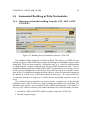
2. Go to the directory arp_warp_7.5 and run there the install.sh script by simply typing
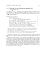
% ./install.sh
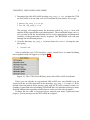
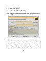
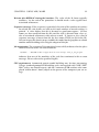
After installation, the CCP4 interface, ccp4i, should have its model building
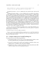
menu updated and will appear as in figure 2.1.
Figure 2.1: The CCP4i Model Building menu after ARP/ wARP installation
Unless you are already an experienced ARP/ wARP user, you should try to get
started with the test files provided in the directory arp_warp_7.5/examples. These
include data for protein chain tracing (also with NCS), helix/strands search, nucleotides, ligand and solvent building. README files are included which give more
detailed information regarding which data are to be used for what purposes.
If things do not work as expected please consult your more experienced colleagues, system manager or the ARP/ wARP developers.
CHAPTER 2. INSTALLING ARP/ WARP
2.2.1
9
Installing for Multiple users
The recommended way to install ARP/ wARP, so that it can be shared by multiple
users, is by doing a command line install. The user who is doing the installation
should have both write permission to the installation directory and write permission
to the CCP4 installation directory.
%
%
%
%
gunzip arp_warp_7.5.tar.gz
tar xvf arp_warp_7.5.tar
cd arp_warp_7.5
./install.sh
At the end of the installation, the CCP4 startup files will be updated with an
addition similar to following lines:(for c-shell)
## Line below added by \emph{ARP/\,wARP} 7.5 installer
[ -r /destination-ccp4/bin/arpwarp.source-csh ] &&
source /destination-ccp4/bin/arpwarp.source-csh
where destination-ccp4 is the $CCP4 directory. The file /destination-ccp4/
bin/arpwarp.source-csh will be created and will contain the following instruction
[ -r /destination-arpwarp/arpwarp_setup.csh ] &&
source /destination-arpwarp/arpwarp_setup.csh
where /destination-arpwarp is the location where ARP/ wARP was installed.
2.3
Installation of ARP/ wARP-CCP4 as a bundle
ARP/ wARP can be installed together with CCP4 by downloading the joint bundle,
directly from the CCP4 web site. Both packages can be obtained and installed with
a single mouse click.
3
Using ARP/ wARP
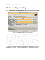
3.1
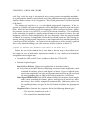
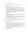
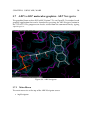
3.1.1
Automated Model Building
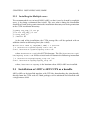
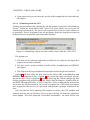
Running protein model building from the GUI, ARP/ wARP
Classic
Figure 3.1: Protein model building using ARP/ wARP Classic from the CCP4 GUI
This module of ARP/ wARP provides automated protein model building starting
from experimental phases or an existing model (molecular replacement), the socalled warpNtrace protocol.
This module aims to deliver an essentially complete model and an improved
density map by utilising the idea of the hybrid model. warpNtrace keeps whatever was recognised as protein (in a form of polypeptide fragments) and the rest
as free atoms and refines this hybrid model during a ‘big’ cycle, consisting of several (default is 5) ARP/ wARP-REFMAC update/refinement cycles. At the end of
10
CHAPTER 3. USING ARP/ WARP
11
each ‘big’ cycle the map is interpreted anew using pattern=recognition methods new polypeptide model is constructed and, if the protocol converges right direction,
contains more residues in less fragments. This whole procedure is iterated (default
is 10 times).
The output of warpNtrace is a set of refined polypeptide fragments. If the sequence is available, the traced fragments will be docked in sequence and side chains
built. After the last building cycle the fragments will be arranged to form a globular structure (or, for a case of NCS, several NCS-related structures). The remainder
of the structure (cis-prolines, poorly ordered loops and terminal residues for each
fragment) will have to be completed by the user manually. Since the output model
is refined, its accuracy is comparable to that of the refined structure. Mis-tracing (incorrect tracing of polypeptide fragments) is not impossible but should normally be
a small part of the structure. An estimate of the correctness of the model is printed
after every model building cycle (the accuracy of this estimate is about 2.5
% Chains 12, Residues 434, Estimated correctness of the model 99.1 %
Below the use of the module for a start from a density map is described in detail, input in case of molecular replacement model is very similar and should be
straightforward to figure out.
• Launch the ARP/ wARP Classic window within the CCP4i GUI.
• Provide required input:
Run ARP/ wARP for Choose the application as described above.
in X-ray data in the MTZ format containing structure factor amplitudes, their
standard deviations, phases and figures of merit. If pre-weighted structure factor amplitudes are to be used to construct initial map, please check
the corresponding box in ARP/ wARP flow parameters (see below).
Fobs Sigma PHIB FOM If the MTZ column labels for structure factor amplitudes, their standard deviations, phases and figures of merit have obvious names, they will be recognised automatically. Otherwise please use
the scrolling button, navigate to List All Labels and chose the appropriate
ones.
Sequence file in Provide the sequence file in the following format (pir):
– The first line should start with ‘>’
– The second line should be blank
CHAPTER 3. USING ARP/ WARP
12
– The sequence (1 letter code) starts from the third line. The space characters hereafter are ignored.
– In the case of heteromers, separate different sequences with around
10 alanines.
Dock the autotraced chains Should the sequence be not available, please uncheck this box in ARP/ wARP flow parameters.
Total residues in the AU / number of molecules Provide the total number of
residues in the asymmetric unit. ARP/ wARP may be able to correct obvious mistakes, but it will not replace a human brain. The number of
molecules is obviously 1 for a monomer. In a case of NCS the number
molecules should be the number of NCS related molecules (e.g. if you
have 2 molecules in the AU with 200 residues each, enter 400 for the total number of residues and 2 for the number of molecules). If you have a
hetero-multimer, e.g. 3α/3β structure, the NCS order is 3 but please make
sure that the sequence file contains both α and β sequences separated by
about 10 alanines:
SEQUENCE OF α SUBUNIT AAAAAAAAAA SEQUENCE OF β SUBUNIT
Cycles of autobuilding / total cycles The default is 10 building cycles separated with 5 ARP/ wARP-REFMAC atom update a refinement cycles (thus
making 50 cycles in total). In cases of good starting phases the autobuilding may converge faster; in cases of poorer phases more cycles may be
required. You can always submit warpNtrace for further cycles using the
output of the previous tracing (protocol automated model building starting from existing model).
Protocol for REFMAC5 / Rfree The refinement target gives three choices:
1. The default is to use maximum likelihood target.
2. The second choice allows the user to use the SAD target. This function is based on REFMAC5 developments by Skubak & Pannu, and
allows to refine against the F+/F- data, when these are available. A
prerequisite when this option is activated, is to also provide a PDB file
with the anomalous scatterers, and define the extent of the ‘anomalous signal’ either by providing the wavelength, or measured f 0 and
f 00 values. Currently ARP/ wARP accepts only one type of atom to
be defined when f 0 , f 00 values are used. If you have more than one
atom, you just choose the wavelength to fetch theoretical values - that
should in practice work well.
CHAPTER 3. USING ARP/ WARP
13
3. The third choice is the ’Phased ML’ function, which is not recommended to use with SAD data. If MAD or MIRAS data are available,
you should use ’Phased ML’ in conjunction with good quality phase
error estimates in the form of HL coefficients.
The default is not to use Rfree, since the number of traced residues serves
as excellent indicator of the success of the job. You can certainly turn the
use of Rfree on.
• Click on Run and choose Run now.
There are a number of additional parameters that you normally should not worry
about. A brief description is given below.
• ARP/ wARP flow parameters:
Use conditional restraints for free atoms This allows restraints to be used to
keep free atoms in reasonable places. The default is on.
Use Non-Crystallographic Symmetry Restraints Indicate to REFMAC that it
˚ or better this is on by
should use NCS restraints. At resolution 1.5 A
default.
Use Non-Crystallographic Symmetry information to extend chains Extend
chains using information provided by related parts of the structure. At
˚ or better this is on by default.
resolution 1.5 A
Use Loopy to build loops This option allows the loop-filling mode to be invoked throughout the iterations. The default is on.
Dock the autotraced chains to sequence The default is to dock the fragments
starting from building cycle 0.
Se-Methionine If you have Se-methionine substituted protein, regardless of
the use of the refinement function, you can check the box thus asking
ARP/ wARP to build and refine Se-Met residues.
Search for helices and strands before each building cycle This is the default
˚ or worse. Should the model from helix/strands
for resolution of 2.7 A
tracing be more complete than the model from warpNtrace, the appropriate message will be printed at the end of the short log file.
Pre-weighted Fobs for initial map calculation Checking this box will result
in a pool-down menu asking for the FBEST label.
CHAPTER 3. USING ARP/ WARP
14
Number of ARP/REFMAC refinement cycles between autobuilding The default is 5. In cases of poor convergence you can try to increase this number
to 10.
Skip the autobuilding for the first cycles Checking this box will disable the
autotracing for the provided number of cycles. This was sometimes advantageous with earlier ARP/ wARP versions when the initial phases were
poor.
Randomisation of atomic positions This also was sometimes advantageous
with earlier ARP/ wARP versions when the initial model bias was high.
The default is not to randomise.
Iterate the tracing Each protein chain tracing is carried out in several rounds
against the same density map. The default number of rounds is 5 and it
is not recommended to change this value.
Density thresholds for atom removal and addition
These parameters are
fixed to 3.2 and 1.0, respectively. In cases of poor convergence, particularly when the number of both added and removed atoms is considerably less than the number requested (as can be seen from the log file), the
threshold for atom removal can be slightly increased. Also, at resolution
˚ and lower it may be advantageous to decrease the threshold for
of 2.5 A
atom addition from 3.2 to 3.0 or 2.8.
Change the number of atoms to be added and removed The default is 1 (no
increase) and it is not recommended to change this.
Disable Wilson plot statistics check The current Wilson plot checking routine is probably too stringent. You may disable the check and the warnings if you are sure that the X-ray data is of high quality. However, we
strongly recommend not to disable the check and in case of warnings,
inspect the plot and only then proceed.
• REFMAC parameters:
Attempt to correct for data collected from a twinned crystal REFMAC will attempt fully automated twinning. This option is incompatible with SAD
refinement.
Cycles of refinement in each REFMAC run REFMAC is invoked to refine the
hybrid model before the density maps are computed. The default is 1 cy˚ or better, otherwise 3 cycles.
cle if the data extend to a resolution of 2.3 A
There is usually no need to change this parameter.
CHAPTER 3. USING ARP/ WARP
15
Damp shifts The default is 1.0 for both types of shifts. There is usually no
need to change these parameters.
Matrix weight for Xray / Geometry The default is automatic weighting. This
proved to work well.
Scaling model The default is to use simple scaling of the low angle part of the
X-ray data. You can change this to bulk solvent correction if you are sure
˚ resolution are complete and
that your low angle data below about 8 A
correct.
Scaling B factor The default is to use anisotropic B factor for scaling the X-ray
data. You can choose isotropic scaling B factor if your data are systematically incomplete (e.g. a cone is missing in reciprocal space).
Free R label This option appears if the free R flag has been chosen for refinement of the protein part of the model. Here you can provide a column
label for the free R flag.
Use of free R reflections This option also appears if the free R flag has been
chosen. The scaling and calculation of σA coefficients by REFMAC can be
computed on the basis of the free reflections (this is the default) or using
all reflections.
Solvent mask correction The default is to use solvent mask correction in REFMAC.
• Crystal parameters:
Space group, Cell, ARP/ wARP asymmetric unit Wilson B factor and Solvent
content are derived automatically from the MTZ file and the total number
of residues in the asymmetric unit. They are displayed for information
only and cannot be changed. However, you may want to check whether
their values conform to your expectations. If the solvent content is outside
of the expected limits, ARP/ wARP may be able to correct this automatically during the run.
Resolution By default all data present in the MTZ file will be used. You can
check the box and then narrow the range if you are aware of certain deficiencies of your data.
• Submit a remote job at the Hamburg Cluster:
– Checking this button will activate remote submission. This is described
below in a separate chapter.
CHAPTER 3. USING ARP/ WARP
3.1.2
16
Command line model building, auto tracing.sh
The script auto_tracing.sh in the $warpbin directory allows running the automated model building from the command line without the use of the GUI. The use
of auto_tracing.sh is fairly simple. If invoked without arguments the script will
print help information.
Usage:
auto_tracing.sh
datafile {mtzfile}
[residues {number_of_residues_in_AU}]
[workdir {FULLPATH_WORKING_DIRECTORY}]
[fp {fp_label}] [sigfp {sigfp_label}] [freelabin {freer_label}]
[fbest {weighted_amplitude_label}] [phibest {phibest_label}] [fom {fom_label}]
[modelin {input_PDB_file_to_use_as_initial_model}]
[seqin {sequence_file_for_one_NCS_copy}]
[cgr {number_of_NCS_copies (if seqin is provided, default is 1) }]
[buildingcycles {the_number_of_autobuilding_cycles (default is 10) }]
[resol {’rmin rmax’ (default is the full resolution range) }]
[albe {1 to always invoke albe, default is 0 for resol < 2.7A, else 1) }]
[restraints {1 to use conditional restraints, default is 1 }]
[twin {1 to try de-twining and twin refinement, default is 0 }]
[sad {1 to turn on the SAD function refinement,
needs also ’wavelength’ and ’heavyin’ on input, default is 0 }]
[compareto {PDB_file_for_comparison}]
[keepjunk {1 to keep intermediate models, default is 0 ]
[parfile {parfilename_if_only_parfile_is_to_be_created}]
\
\
\
\
\
\
\
\
\
\
\
\
\
\
\
\
\
\
\
- Optional command line arguments are given in square parentheses
- Possible combinations of MTZ labels are:
For start from phases:
fp/sigfp/phibest/fom or fbest/sigfp/phibest to build initial free-atoms model
and fp/sigfp to refine the model
If ’fbest’ is given, ’fom’ will be ignored
For start from a model:
fp/sigfp to refine the model
- All input files are assumed to be located in working directory
unless they are given with full path
- If workdir is not given, the current directory will be assumed
- All output files will be written into workdir/subdirectory
Additional useful tips:
- Normally the job runs in a subdirectory called YYYYMMDD_HHMMSS
To run the job in the current directory use: auto_tracing.sh jobId ’.’
- If you invoke auto_tracing.sh from another script and the keywords with
double-word argument are not properly understood, e.g. resol ’20.0 2.5’,
try resol 20.0;2.5 or resol ’20.0;2.5’
- If you have a par file from an earlier version of \emph{ARP/\,wARP} and would like to
re-run that job now, use: auto_tracing.sh defaults OLD_PAR_FILE
This will create a par file compatible with the current \emph{ARP/\,wARP} version
and the keywords, which are new to OLD_PAR_FILE will take their default values
- NCS-based chain extension and NCS restraints with REFMAC are applied
automatically if the resolution of the data is equal to or lower than 2.1 A.
CHAPTER 3. USING ARP/ WARP
17
Input ’ncsextension 1/0’ to apply / not apply NCS extension regardless of the
resolution of the data. Input ’ncsrestraints 1/0’ has similar effect
Required keyword is: datafile (followed by the mtz-file name with the full
path).
Optional keywords include: residues (followed by the number of residues),
workdir (followed by the absolute path to the working directory), fp (followed by
the fp label), sigfp (followed by the sigfp label), freelabin (followed by the Rfree
label), fbest (followed by the label for the fom-weighted structure factor amplitudes
to be used for initial map calculation), phibest (followed by the best phi label), fom
(followed by the figure of merit label), modelin (followed by a starting pdb-file with
the full path), seqin (followed by a sequence-file name with the full path), cgr (followed by a number of NSC-related copies), buildingcycles (followed by the number of building cycles), resol (followed by the resolution limit), albe (followed by
the flag to enable or not helix/strands building), similarly for restraints, twin and
sad. There are additional parameters, which can be customised, and an experienced
user should have no problem in figuring out how to do this. Alternatively, please
contact the ARP/ wARP developers for advice.
If auto_tracing.sh is called with an option parfile, the script will create a parameter file and a directory in the workdir whose name will be printed. The job can
subsequently be launched by:
% $warpbin/warp_tracing.sh NAME_OF_PARFILE
If auto_tracing.sh is called without an option parfile, it will also launch the
job. The log files and additional output files as well as the building results can be
found in the directory created.
3.1.3
Remote submission of a model building task
This option offers you the following possibilities:
1. Your model building will run using external computational facilities, where
the CPU performance may be superior to your local installation.
2. You can be assured that the most recent working executables will be used,
should you have a problem with your local installation.
3. Should the task stop, an automatic notification will be forwarded to the ARP/
wARP developers who can then promptly help you.
CHAPTER 3. USING ARP/ WARP
18
4. Upon your wish you can share the results of the completed task with software
developers.
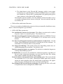
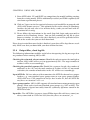
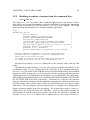
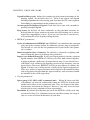
3.1.3.1
Submitting from the GUI
Clicking on the button with “Submit the job for remote execution at the Hamburg
cluster” within the main ARP/ wARP Classic GUI panel allows one to execute an
autotracing task remotely. The panel will expand and ask for an email address to
be provided. Please also choose one of the options from the drop down menu to
indicate how you would like your data to be handled.
Figure 3.2: Submitting a job to the ARP/ wARP cluster from the CCP4 GUI
The options are:
1. The data can be archived and made available to any software developer that
requests them (this is default).
2. The data can be made available to ARP/ wARP, AutoRickshaw or REFMAC
developers.
3. The data must be kept confidential and deleted after the job has finished.
Option 2 will only allow the data share to the ARP/ wARP, Auto-Rickshaw and
REFMAC development teams. Option 1 will extend the share to anyone who requests the data. In case of option 3 only the short log file, Wilson/omega log files
and the parameter file will be kept by the ARP/ wARP developers, all other data (input PDB, PIR and MTZ files) as well as log files will be automatically deleted one
week after the job has finished. In case of any option the ARP/ wARP developers
may inspect the data in case of a job crash and provide a prompt feedback to the
user.
Once the job has been submitted for remote execution, the GUI window will
indicate that the job has finished. Please inspect the log file from the pull-down
menu option “View files from job” for further instructions. An email will be sent
CHAPTER 3. USING ARP/ WARP
19
to you at the email address that you entered in the GUI window. Please follow the
instructions in the email (http link, login and password) to connect to the Hamburg
cluster. You can then monitor the log file in your browser window. As soon as the
job is finished, you will be provided with a link to the results that you can then
download. please keep in mind that once the job is finished, your data will be kept
for one week only. Make sure that you download your data within that time.
The remote job submission relies on the curl software installed at your site. Availability of curl is checked while installing ARP/ wARP and a warning is given if curl
is not available.
3.1.3.2
Submitting from a web browser
Navigate your browser to:
• http://cluster.embl-hamburg.de/ARPwARP/remote-http.html
or choose model building via the web at:
• http://www.arp-warp.org
1. View the Disclaimer and agree to the ARP/ wARP and the CCP4 licensing conditions.
2. Proceed with the remote services to Step One.
3. Choose the model building protocol (start from experimental phases or existing model).
4. Enter your Email address to which instructions on how to view the results will
be send.
5. Provide your MTZ file by using the ‘Browse’ button, the file must have an
extension .mtz.
6. Click ‘Proceed to Step Two’.
7. Enter starting model (unless you have chosen a protocol to start from experimental phases).
8. Enter the total number of residues and the number of chemically identical molecules in the asymmetric unit. Please make sure you enter these two numbers
right. If, for example, the asymmetric unit contains a dimer with each subunit
having 50 residues, then you enter 100 and 2, respectively.
CHAPTER 3. USING ARP/ WARP
20
9. Enter MTZ labels. FP and SIGFP are compulsory for model building starting
from the existing model. PHI is additionally needed (and FOM is optional) for
start from experimental phases.
10. Click on ‘I agree to cite the required references and would like to proceed with
ARP/ wARP remote services’. This uploads the files to the cluster in Hamburg,
launches the job and, after a few minutes delay, sends you an Email with instructions for viewing.
11. Please follow the instructions in the email (http link, login and password) to
connect to the Hamburg cluster. You can then monitor the log file in your
browser window. As soon as the job is finished, you will be provided with a
link to the results that you can then download.
Please keep in mind that once the job is finished, your data will be kept for one week
only. Make sure that you download your data within that time.
3.1.4
Output files, short log file
The following information could be useful when interpreting the log messages that
are produced when running ARP/ wARP.
Checking the estimated solvent content Should the solvent content be too high or
too low, ARP/ wARP will re-set it to approximately 50%. The target number of
residues will be reset accordingly.
Checking the provided sequence file Should the sequence length, the number of
molecules in the AU and the total number of residues in the AU not match
each other, the number of molecules in the AU will be reset accordingly.
Input MTZ file We have observed that sometimes the MTZ files do not have proper
headers, e.g. non-standard space group name or zero space group number.
ARP/ wARP uses CAD program to always do a header fix, thus the MTZ file
may have an extension .mtz.cad.
Space group number ARP/ wARP supports all standard non-centrosymmetric space
groups, P1bar and several non-standard space groups (e.g. 1017 or 2017). The
space group is figured out solely from the symmetry operators stored in the
MTZ file header.
Input files The ASCII files (sequence, input PDB or input file with heavy atoms) are
always converted to a Unix line feed, thus they have an extension _lf.
CHAPTER 3. USING ARP/ WARP
21
Checking whether input PDB contains ligands This check comes up if the initial
model is available. Should the model contain ligands unknown to the REFMAC library, they are renamed to free DUM atoms. This should not affect the
model building performance, but the warning is printed.
R factor after REFMAC before model building If the initial model is available, a
number of restrained refinement cycles with REFMAC is carried out until R
factor convergence.
Building cycle one Normally one should expect a considerable part of the structure built already at the starting building cycle. If this is not the case, observe
the situation for a few further building cycles. If, however, there is essentially
nothing autotraced for further building cycles, please inspect whether the initial phases are sufficiently good or the space group is correct.
Search for helices and strands The module for building helical and beta-stranded
˚ resolution
fragments is invoked if requested or by default with data at 2.7 A
or lower. The number of built helical/stranded residues and chain fragments
is printed.
Rounds within building cycle Each cycle of the main chain tracing is carried out
in several rounds. Normally each successive round should result in more
residues and in fewer fragments. The maximum length of the traced fragment
and the tracing score of the model built are also printed for information. The
tracing score is on an arbitrary scale, but the higher it is the better.
Chains, residues and estimated correctness of the model The output from the best
tracing round is processed further. Fragments of 4 residues or shorter as well
as the terminal residues of the fragments are converted to free atoms. The rest
is used to provide restraints for subsequent ARP/ wARP-REFMAC cycles. The
value of the estimated correctness of the model should steadily approach 100%
if the tracing is successful.
Residues docked into sequence If the sequence is provided, the autotraced fragments are docked into it and the side chains are built and refined in real space.
The results are printed out. If the sequence is not provided, side chain guesses
only (GLY/ALA/SER/VAL) are built and refined.
Loop building This is invoked if the sequence is available and if the tracing score
is above 0.85. It is also invoked after the last building cycle.
CHAPTER 3. USING ARP/ WARP
22
R factor after REFMAC during the iterations The value of the R factor typically
oscillates. At the end of the procedure it should reach a value typical for a
restrained refinement.
Sequence coverage If the sequence is provided, the ratio of the number of residues
for which the side chains are built to the total number of traced residues is
printed. A value higher than 0.8 is deemed as good convergence. All free
atoms are then removed from the file and the task is directed into a few cycles of restrained refinement with solvent search. If, however, the value of
sequence coverage is lower than 0.8, the free atoms (DUM) are left in the file.
You can inspect the density maps, modify the model on the graphics or submit
another model building task using the output of this job.
Job termination The statement Task completed successfully indicates that the job is
finished with no error. An error statement:
QUITTING ... ARP/wARP module stopped with an error message: name_of_the_program
indicates that one of the modules of the task has terminated with an error
message. Please refer to the specified log file.
CPU requirements Automated protein model building may be time consuming.
Using a standard protocol of 10 building cycles interspaced with 5 ARP/ REFMAC cycles, one should expect a job for a structure of 500 residues to be completed within about 1 hour (subject to the power of the computer you are using).
CHAPTER 3. USING ARP/ WARP
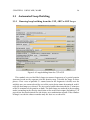
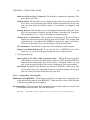
3.2
3.2.1
23
Automated Construction of Helical and
Beta-Stranded Fragments
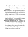
Building secondary structure from the GUI, ARP/ wARP
Quick Fold
Figure 3.3: Running Quick Fold from the CCP4 GUI
The procedure for building secondary structural elements is based on the use of
discriminant analysis in a successive filtering scheme taking into account the geometry of alpha-helical and beta-stranded main-chain fragments. The built fragments
are then regularised and the chain direction is chosen on the basis of their fit to the
density. Finally the fragments are refined in real space.
The accuracy of the resulting model depends on many parameters. The module
˚ However, it
should be able to build helices and strands at resolutions as low as 4.5 A.
may not result in complete helical/stranded structure and it may also contain parts
that are mis-interpreted. The expected top performance is the correct location of
90% of the helices and 50% of the strands. The procedure is relatively fast and takes
only seconds to minutes for proteins of moderate size (up to 500 residues).
The secondary structure recognition module is optimised to address lower resolution data and hard cases where, e.g. the full model building protocol has not been
˚ the module will automatically trim
successful. For a resolution higher than 2.6 A
the resolution and Wilson B-factor of the data to approach its design conditions.
CHAPTER 3. USING ARP/ WARP
24
• Launch ARP/ wARP Quick Fold window within the CCP4i GUI.
• Provide required input:
MTZ in X-ray data in the MTZ format containing structure factor amplitudes
and their standard deviations, phases and foms.
Fobs Sigma Phib FOM If the MTZ column labels for structure factor amplitudes, their standard deviations, phases and figures of merit have obvious
names, they will be recognised automatically. Otherwise please use the
scrolling button, navigate to List All Labels and choose appropriate ones.
Output PDB file Provide the PDB file name where the constructed secondary
structure fragments will be output to.
• Set parameters:
Number of residues Provide the expected number of residues in the asymmetric unit. This is optional but, if given, should be a good guess within
± 20% of the true number.
Do NOT build beta-strands If you have real doubts about your structure having a fold with a significant content of beta-strands, you can deactivate
their construction by checking the box.
• Now you are ready to start the job: Click on Run and choose Run now.
There are a number of additional parameters that you normally should not worry
about. A brief description is given below:
• Crystal parameters:
Space group, Cell, ARP/ wARP asymmetric unit , Wilson B factor and Solvent content are derived automatically from the MTZ file and the total
number of residues in the asymmetric unit. They are displayed for information only and cannot be changed. However, you may want to check
whether their values conform to your expectations.
Resolution By default all data present in the MTZ file will be used. You can
check the box and then narrow the range if you are aware of certain deficiencies of your data.
• Coordinate comparison:
CHAPTER 3. USING ARP/ WARP
25
Compare with an already deposited protein for validation or testing If you
have the final model and would like to check the installation and the performance of the software, you can check this box. You will then have to
provide a PDB file that will be used for comparison.
3.2.1.1
Output files, short log file
The following information could be useful when interpreting the log messages that
are produced when running Quick Fold.
Checking the estimated content Should the solvent content be too high or too low,
ARP/ wARP will re-set it to approximately 50%. The target number of residues
will be reset accordingly.
Residues and chain fragments The important numbers are highlighted in red and
bold in the short log file, indicating the number of residues and the number
of fragments into which these residues are arranged. The higher the values of
the Connectivity index and the Tracing score, the more complete and reliable
the resulting model is. The length of the longest chain is also printed.
Further extension of the model You may try to feed the PDB output of the module
into the Classic model building. However, subject to the resolution of the data,
this may not provide enough seed for subsequent automatic tracing of the full
chain.
Job termination The statement Task completed successfully indicates that the job
has finished with no error. An error statement:
QUITTING ... ARP/wARP module stopped with an error message: name_of_the_program
indicates that one of the modules of the task has terminated with an error
message. Please refer to the specified log file.
CHAPTER 3. USING ARP/ WARP
3.2.2
26
Building secondary structure from the command line,
auto albe.sh
The script auto_albe.sh (where ’albe’ stands for alpha-beta) in the $warpbin directory allows you to run the secondary structure building as a single-line command
without the use of the GUI. The use of auto_albe.sh is fairly simple. The script
prints out help information if it is invoked without arguments.
Usage:
$warpbin/auto_albe.sh
datafile {mtzfile}
[residues {number_of_residues_in_AU}]
[workdir {FULLPATH_WORKING_DIRECTORY}]
[helixfileout {output_PDB_file}]
[jobId {desired_job_id_used_for_subdirectory_naming}]
[fp {fp label} sigfp {sigfp label} phib {phi label}]
[fom {fom label}] (input ’fom none’ if no fom is to be used)
[compareto {PDB_file_for_comparison}]
[nostrands {0 or 1, default=0}]
[parfile {parfilename_if_only_parfile_is_to_be_created}]
\
\
\
\
\
\
\
\
\
\
- Optional command line arguments are given in square parentheses
- All input files are assumed to be located in working directory
unless they are given with full path
- If workdir is not given, the current directory will be assumed
- All output files will be written into workdir/subdirectory
Required keyword is: datafile (followed by the mtz-file name with the full
path).
Optional keywords include: residues (the expected number of residues in the
asymmetric unit), workdir (followed by the full path to the working directory),
helixfileout (the name of the PDB file where the traced both helical and stranded
fragments will be output to), jobId (if you wish that the working sub-directory has
a particular name), fp (followed by the fp label), sigfp (followed by the sigfp label),
phib (followed by phibest label) and fom (followed by the label to fom). The defaults
are FP, SIGFP, PHI and FOM, respectively. Alternatively, if the mtz file contains
only one column for structure factor amplitudes and only one column for their standard deviations, these will be taken. If you wish FOM not to be used, please input
’fom none’. For test purposes, the constructed helices/strands can be compared to
known reference models (hand- or pre-fitted). The required keyword is compareto
(followed by the full-path name of a PDB file). You can also enable/disable the
construction of strands using the keyword nostrands, the default is 0 (build the
strands). If auto_albe.sh is called with an option parfile, the script will create a
CHAPTER 3. USING ARP/ WARP
27
parameter file and a directory in the workdir whose name will be printed. The job
can subsequently be launched by:
% $warpbin/warp_albe.sh NAME_OF_PARFILE
If auto_albe.sh is called without an option parfile, it will also launch the job. The
log files and additional output files as well as the building results can be found in
the directory created.
CHAPTER 3. USING ARP/ WARP
3.3
3.3.1
28
Automated Loop Building
Running loop building from the GUI, ARP/ wARP Loops
Figure 3.4: Loop building from the CCP4 GUI
This module tries to find likely loops to connect fragments of a partial protein
structure based on the sequence and the density map. It builds the loops in three
phases. First a tree of possible Cα atoms between the fragments is build, next the
unlikely ones are removed and the rest of the main chain atoms determined, and finally the best loops are selected. The tree can be build either towards the C-terminus
of the N-terminus of the protein, or both. The built loops are ordered (in descending
order) according to the density correlation at the main chain atoms (including Cβ if
present) or the correlation of the side chains, or a combination of both. If the number
of loops exceeds the chosen number only the best are saved to file.
CHAPTER 3. USING ARP/ WARP
29
• Launch the ARP/ wARP Loops window within the CCP4i GUI
• Provide required input:
Building loops Select whether to start from a map or an mtz file.
Mode loop building Select whether to try to build all loops in the PDB file (a
sequence file will be needed) or to build a specific loop
MTZ in X-ray data in the MTZ format containing structure factor amplitudes
and their standard deviations.
Fmap PHImap If the MTZ column labels for structure factor amplitudes and
their standard deviations have obvious names, they will be recognised
automatically. Otherwise please use the scrolling button, navigate to List
All Labels and chose appropriate ones.
Protein model for loop building Provide the PDB file with coordinates of the
protein. Note that the module will only attempt to build missing loops
and will not rebuild any of the existing residues.
New loops output file Provide the name of the PDB file where the built loops
will be written to.
Protein and new loops combined output Provide the name of the PDB file
where the protein model together with the built loops will be written to.
• Click on Run and choose Run now
There are a number of options that can be added. A brief description is given
below.
• Definition of loop:
Build a loop Provide anchor residues of a fragment on the N and the C terminus side of the protein. If you want to rebuild some terminal residues,
you need to remove them from the input PDB file. Provide the length of
the loop including the two anchor points.
• Selecting best loops:
Deviation distance loop connection Set the allowed error in the Cα-Cα distance.
Cα density correlation threshold This number sets the number of best loops
kept based on the density correlation of the Cα atoms only.
CHAPTER 3. USING ARP/ WARP
30
Structural threshold Set the threshold for the minimal value for the log likelihood of this structure. Set the minimum value, if you want to ensure to
keep at least a certain number of loops after pruning. Set the maximum
value, if you want to ensure that the number of loops doesn’t exceed a
certain amount after structural pruning.
Main chain density correlation This parameter sets the number of best loops
kept.
• Selecting best Cα atoms:
Likelihood threshold This is the threshold for a Cα to represent the fifth Cα of
a penta-peptide, based on density correlation, Cα-Cα distance and structure.
Minimum distance Cα atoms Measures the minimal distance between Cα atoms
from the same shell. The Cα with the best likelihood is kept.
• Generating Cα atoms:
Select generation Cα shell By default a shell with a uniform and regular distribution of Cα atoms at exactly Cα-Cα distance is generated. You can
also choose for a uniform and random distribution of the Cα atoms. In
that case, the shell is generated with a given thickness.
Number of Cα atoms Number of Cα atoms generated within a shell.
Cα-Cα distance Distance to use between successive Cα atoms.
Keep Cα atoms with negative density halfway Default for this option is not
to keep the atoms.
• Crystal parameters:
Space group and Cell are derived automatically from the MTZ and the PDB
files, displayed for information only and cannot be changed. However,
you may want to check whether their values conform to your expectations.
• Log files of Loopy:
Message level Choose a value between 0 and 9, the default is 4
Abort level If a message at this level is encountered, the module will abort.
The default value is 8.
CHAPTER 3. USING ARP/ WARP
Message file Name for the message file (plain text).
XML output file Name for the XML message file (xml format).
31
CHAPTER 3. USING ARP/ WARP
3.4
3.4.1
32
Automated Building of Poly-Nucleotides
Running nucleotide building from the GUI, ARP/ wARP
DNA/RNA
Figure 3.5: Building Poly-Nucleotides from the CCP4 GUI
This module builds fragments of DNA or RNA. The input is an MTZ file containing the phases from which the map best describing the nucleotide region can be
computed. Thus the map could be a difference map (e.g. after the protein model
is completed) or a sigma-weighted map for the whole asymmetric unit. The nucleotide building procedure within ARP/ wARP 7.5 proceeds in several steps: first it
locates putative phosphates in the density map, then uses them in a manner analogous to the CA-candidates for protein chain tracing. After the nucleotide fragments
are obtained, a likely base is built and refined in real space. The type of the base
is currently limited to A (large) or C (small) and the nucleotide sequence is not yet
used.
The produced poly-nucleotides are quite accurate, a typical r.m.s.d. for the built
˚ with X-ray data extending to around 3.0 A
˚ resolution. The
backbone atoms is 0.6 A
method is not sensitive to a particular DNA or RNA conformation. The module is
not very CPU efficient and may take about 10 minutes for a 20-nucleotide structure.
• Launch the ARP/ wARP DNA/RNA window within the CCP4i GUI
• Provide required input:
CHAPTER 3. USING ARP/ WARP
33
MTZ in X-ray data in the MTZ format containing structure factor amplitudes
and their standard deviations.
Fobs Sigma PHIB FOM If the MTZ column labels for structure factor amplitudes and their standard deviations have obvious names, they will be
recognised automatically. Otherwise please use the scrolling button, navigate to List All Labels and chose appropriate ones. FOM is optional and
could be omitted if Fobs are already FOM-weighted.
Output PDB file Provide the PDB file name where the constructed polynucleotide fragments will be output to.
• Click on Run and choose Run now
There are a number of options that can be added. A brief description is given
below.
• Space group, Cell, ARP/ wARP asymmetric unit, Wilson B factor and Solvent
content are derived automatically from the MTZ file and the total number
of residues in the asymmetric unit. They are displayed for information
only and cannot be changed. However, you may want to check whether
their values conform to your expectations. Obviously, if you entered zeros as the expected number of residues and nucleotides, the solvent content will be displayed as 1.0 but you should not worry about this.
Resolution By default all reflections present in the MTZ file will be used. You
can check the box (Use reflections between) and then narrow the range if
you are aware of certain deficiencies of your data.
3.4.1.1
Output files, short Log File
The following information could be useful when interpreting the log messages that
are produced when building DNA/RNA.
Checking the estimated content Should the solvent content be too high or too low,
ARP/ wARP will re-set it to approximately 50%. The target number of residues
will be reset accordingly.
Phosphate candidates The identified number of phosphate candidates is typically
100 times higher than the number of nucleotides in the structure.
Nucleotides and chain fragments The important numbers are highlighted in red
and bold in the short log file, indicating the number of nucleotides and the
CHAPTER 3. USING ARP/ WARP
34
number of fragments into which these residues are arranged. The length of
the longest chain is also printed.
Job termination The statement Task completed successfully indicates that the job
has finished with no error. An error statement
QUITTING ... ARP/wARP module stopped with an error message: name_of_the_program
indicates that one of the modules of the task has terminated with an error
message. Please refer to the specified log file.
3.4.2
Running nucleotide building from the command line,
auto nuce.sh
The script auto_nuce.sh in the $warpbin directory allows you to run the secondary
structure building as a single-line command without the use of the GUI. The use of
auto_nuce.sh is fairly simple. The script prints out help information if it is invoked
without arguments.
Usage:
$warpbin/auto_nuce.sh
datafile {mtzfile}
[residues {number_of_protein_residues_in_AU}]
[nucleotides {number_of_nucleotides_in_AU}]
[workdir {FULLPATH_WORKING_DIRECTORY}]
[fp {fp_label}] [sigfp {sigfp_label}] [fbest {weighted_amplitude_label}]
[phib {phib_label}] [fom {fom_label}]
[resol {’rmin rmax’ (default is the full resolution range) }]
[compareto {PDB_file_for_comparison}]
[parfile {parfilename_if_only_parfile_is_to_be_created}]
\
\
\
\
\
\
\
\
\
\
- Optional command line arguments are given in square parentheses
- Possible combinations of MTZ labels for map calculation are:
fp/sigfp/phib/fom or
fbest/sigfp/phib if fbest is already fom-weighted.
- In the latter case, if ’fbest’ is given, ’fom’ will be ignored
- All input files are assumed to be located in working directory
unless they are given with full path
- If workdir is not given, the current directory will be assumed
- All output files will be written into workdir/subdirectory
Required keyword is: datafile (followed by the mtz-file name with the full
path). In difference to the functionality offered from the CCP4 GUI, datafile can
also be a density map.
CHAPTER 3. USING ARP/ WARP
35
Optional keywords include: residues (the expected number of residues in the
asymmetric unit), nucleotides (the expected number of nucleotides in the asymmetric unit), workdir (followed by the full path to the working directory), fp (followed by the fp label), sigfp (followed by the sigfp label), phib (followed by phibest
label) and fom (followed by the label to fom). The defaults are FP, SIGFP, PHI and
FOM, respectively. Alternatively, if the mtz file contains only one column for structure factor amplitudes and only one column for their standard deviations, these will
be taken. If you wish FOM not to be used, please fbest. You can set resol (followed
by the resolution limit). For test purposes, the constructed model can be compared
to known reference model. The required keyword is compareto (followed by the
full-path name of a PDB file).
If auto_nuce.sh is called with an option ‘parfile’, the script will create a parameter file and a directory in the workdir whose name will be printed. The job can
subsequently be launched by:
% $warpbin/warp_nuce.sh NAME_OF_PARFILE
If auto_nuce.sh is called without an option ‘parfile’, it will also launch the job. The
log files and additional output files as well as the building results can be found in
the directory created.
CHAPTER 3. USING ARP/ WARP
3.5
3.5.1
36
Automated Ligand Building
Running ligand building from the GUI, ARP/ wARP Ligands
Figure 3.6: Building Ligands from the CCP4 GUI
The ligand building procedure within ARP/ wARP Version 7.5 proceeds in three
steps: first it locates the binding site in the difference density map, then builds there
a number of putative ligand models and, finally, selects the best model, which is
geometrised and real-space fit into the density.
The binding region may be selected automatically by matching ligands shaperelated properties to the regions of high density. For the construction of the ligand
set two algorithms are used. One exploits the combinatorial assignment of the ligand atom identities to the grid nodes, ‘label swap’. Another algorithm maximises
the overlap between the sparse set and the ligand model by a random search in conformational space. The output from both algorithms is merged and then undergoes
a last stage of real-space refinement before the final model is selected.
The accuracy of ligand building is mainly dependent on ligand size and the resolution of the X-ray data. As a rough guide, about 75% of well-ordered ligands of
CHAPTER 3. USING ARP/ WARP
37
˚
a size around 20 to 40 non-hydrogen atoms should be built within r.m.s.d. of 1.0 A
from their correct location. Thus the constructed models should be accurate enough
for REFMAC5 to straightforwardly refine the protein-ligand complex. The procedure can be iterated to locate additional ligands, if any are present.
The ARP/ wARP ligand building module requires the X-ray data (in MTZ format), the built protein without ligands (in PDB format) and either a template model
of the ligand to build (also in PDB format) or a ligand 3-letter code. Options include
the possibility to specify the binding site, the ability to compare the run result to
some reference ligand(s), and the possibility to build a ligand taken from a list of
candidates (‘cocktail’). In the latter case, the coordinates of the ligand candidates
should be concatenated into a single PDB file. The different ligands must be distinguished by their residue names (columns 18-20), chain identifiers (column 22) or
residue sequence numbers (columns 23-26). ARP/ wARP will automatically choose
the best-matching ligand candidate and will attempt to build it at the binding site,
either determined automatically or supplied by the user. However, since this feature
is new, the specification of the binding site (see below) is recommended. One can
also specify that only well-resolved parts of a partially occupied ligand should be
modelled and indicate the minimum number of atoms present in the bound ligand
fragment. The default is 4 or more atoms.
• Launch the ARP/ wARP Ligands window within the CCP4i GUI
• Provide required input:
MTZ in X-ray data in the MTZ format containing structure factor amplitudes
and their standard deviations.
Fobs Sigma If the MTZ column labels for structure factor amplitudes and
their standard deviations have obvious names, they will be recognised
automatically. Otherwise please use the scrolling button, navigate to List
All Labels and chose appropriate ones.
Protein model without ligand Provide the PDB file with coordinates of the
protein only. If the file contains solvent atoms, free atoms or fragments
of other ligands, please make sure that their location is not overlapping
with the supposed location of the ligand or have them removed prior to
running ligand building.
Ligand molecule Choose whether to input the ligand as a PDB file or using
a 3-letter PDB ligand code. Stereochemical information about the ligand
to be built is normally read from the provided PDB file if input. The
file should contain the ligand molecule only. The molecule can be in any
CHAPTER 3. USING ARP/ WARP
38
conformation, but the interatomic distances, bonding angles and chirality
(if present) should be sensible and correspond to the target stereochemistry of the ligand to be built so that the automated recognition of ligand
topology works. Please also check that there is atom-bonded connectivity
throughout the whole target ligand molecule (i.e. you do not accidentally
have several unconnected clusters of atoms) and that there are no atoms
˚ Otherwise, the restraints
that are too close to each other (distance < 0.6 A)
defined in the REFMAC ligand library file are used if a 3-letter ligand
code is input.
• Click on Run and choose Run now.
There are a number of options that can be added either in the main GUI panel
(scrolling bar Build the ligand) or under the Parameters section. You normally need
not worry about these (except if you want the ligand to be built around a known
location or if you would like to screen a list of candidate ligands, i.e. a ‘ligand
cocktail’). A brief description is given below.
• Optional parameters:
Build the ligand (Binding site location)
In the most likely place of the complete asymmetric unit (default)
around the same approximate place as a previous ligand The binding
site is defined by the position of a compound known to bind at the
desired location. If you use this option, the region is provided by
submitting a PDB file specifying the previous ligand coordinates.
around an approximate XYZ position The binding site is defined by (X,
Y, Z) Cartesian coordinates and an input search radius (option Search
for the ligand around). It is recommended that the user specify a
binding site using this option if partial occupancy of the ligand is to
be assessed.
REFMAC5 By default the fast protocol is used (1 cycle of refinement). If your
PDB file needs considerable pre-refinement with REFMAC before the difference electron density map can be computed, you can choose the slow
protocol (3 cycles of refinement).
Free R Flag By default, the data flagged as an Rfree set are used in REFMAC
refinement. You can choose to use R-free, and this will cause additional
options to appear within the section REFMAC parameters..
CHAPTER 3. USING ARP/ WARP
39
Ligand building cycles defines the number of grid parameterisations of the
binding region. The default value is 2. There is one run of each ligand
building algorithm for each starting grid, therefore the CPU time required
for building is proportional to this number of cycles.
Assume partial occupancy of ligand Check this box if you wish to model a
partially occupied ligand.
Keep waters By default, all water molecules in the provided structure are
deleted from the input structure to ensure that the binding site is not occupied by inappropriate waters. If you are sure that this is not the case,
water molecules can be kept by ticking this box.
• REFMAC parameters:
Cycles of refinement for REFMAC run REFMAC is invoked to refine your protein part of the structure before the difference density map is computed.
The default is 1 cycle for the fast protocol and 3 cycles for the slow protocol, see above.
Matrix weight for Xray / Geometry The default is automatic weighting and
there is normally no need to change this parameter.
Input a user-defined library file In case your input protein is already a proteinligand complex then REFMAC will have to refine both entities together
in order to obtain a difference electron density map. If you already have
a REFMAC-style cif library for ligand(s) present in the structure, you can
input it here. Otherwise, REFMAC will use its own library if it knows the
ligand. If it does not, it will generate a cif file for the ligand and proceed.
If the user wishes to input restraints for the ligand to be modelled rather
than using those detected from the input structure, such restraints should
be included in the cif file input here.
• Crystal parameters:
Space group, Cell, ARP/ wARP asymmetric unit , Wilson B factor and Solvent content are derived automatically from the MTZ file and the total
number of residues in the asymmetric unit. They are displayed for information only and cannot be changed. However, you may want to check
whether their values conform to your expectations.
Resolution By default all reflections present in the MTZ file will be used. You
can check the box (Use reflections between) and then narrow the range if
you are aware of certain deficiencies of your data.
CHAPTER 3. USING ARP/ WARP
40
• Test and comparison parameters:
Compare with an already fitted ligand If you have the final model of the ligand in the correct orientation and would like to check the installation and
the performance of the software, you can check this box. You will then
have to provide a PDB file that will be used for comparison.
3.5.1.1
Output files, short Log File
The following information could be useful when interpreting the log messages that
are produced when building ligands.
Refinement with REFMAC The R factor (and R free if requested) are printed after
refinement of the protein part only with REFMAC. A value higher than about
30% may indicate that the computed difference map may be too noisy for location of the ligand.
The ligandbuild program The mapping of the difference density synthesis parameterised with grid points onto the ligand atoms is run as many times as defined
by the number of ligand building cycles (ligandbuild and M_ligandbuild).
Real space fit Up to 108 top constructed ligand models undergo a real-space refinement with respect to the difference density map. The best solution is output.
If the test and comparison option is selected, the r.m.s.d. to the reference PDB
file (XYZREF) is also printed. There will be a warning given if the stereochemistry of the constructed ligand is poor. Also a warning will be given if the
constructed ligand molecule has severe steric clashes, which may be a sign of
an incorrect ligand building. You may want to inspect the ligand and the density and if there is a clear part of the ligand that is disordered, try to either run
automatic partial ligand building as described above or manually remove it
from the ligand target PDB file and re-run the job.
Job termination The statement Task completed successfully indicates that the job
has finished with no error. An error statement:
QUITTING ... ARP/wARP module stopped with an error message: name_of_the_program
indicated that one of the modules of the task has terminated with an error
message. Please refer to the specified log file.
CHAPTER 3. USING ARP/ WARP
3.5.2
41
Running ligand building from the command line,
auto ligand.sh
The script auto_ligand.sh in the $warpbin directory allows you to run the ligand
building as a single-line command without the use of the GUI. The use of auto_
ligand.sh is fairly simple. The script prints out help information if it is invoked
without arguments.
Usage:
auto_ligand.sh
datafile {either mtzfile or mapfile}
protein {starting_PDB_file_without_ligand}
[ligand {PDB_file_with_ligand_to_fit}]
[ligandcode {3-letter code of a ligand molecule,
the code must be present in the REFMAC library}]
[workdir {FULLPATH_WORKING_DIRECTORY}]
[ligandfileout {output_PDB_file}]
[fp {fp_label}] [sigfp {sigfp_label}] [freer {freer_label}]
[nligandcycles {number_of_ligandbuild_cycles (default is 2)}]
[search_model {PDB_file_with_model_at_expected_ligand_site}]
[search_position {X Y Z}]
[search_radius {radius_in_angstroms}]
[reflist {textfile_with_FULLPATHnames_of_fitted_ligands_for_comparison}]
[extralibrary {user_defined_library_for_REFMAC5}, additionally
if this library contains data for the ligand to be built, then these
paramters are used to derive ligand topology to the highest level
or priority (ahead of REFMAC cif or coordinate-dervied topology)]
[partial {0 for modelling the whole ligand and 4 or higher number to
model partially occupied ligand (giving 4 would mean to consider
4-atoms as the smallest ligand fragment)]
[keepwaters {1 for keeping them before computing the difference map}]
[parfile {parfilename_if_only_parfile_is_to_be_created}]
\
\
\
\
\
\
\
\
\
\
\
\
\
\
\
\
\
\
\
\
\
\
- Optional command line arguments are given in square parentheses
- All input files are assumed to be located in working directory
unless they are given with full path
- If workdir is not given, the current directory will be assumed
- All output files will be written into workdir/subdirectory
- If no ligand is specified then auto identification of
the ligand will be attempted provided that a search position
is given (experimental)
Required keywords are: datafile (followed by the mtz-file name with the full
path or a map file in CCP4 format) and protein (followed by the pdb-file name
of the protein model without the ligand with the full path). Either the keyword
ligand (followed by the full path to the pdb-file containing the ligand coordinates)
or ligandcode (followed by the 3-letter code of the ligand to be modelled) are normally provided to indicate the nature of the ligand to be built. If they are not spec-
CHAPTER 3. USING ARP/ WARP
42
ified, automated identification of the ligand is attempted, with a database of 84 of
the most common ligands in the PDB being screened. Note that datafile can also
be a density map, an option not offered in the CCP4 GUI.
Optional keywords include: workdir (followed by the full path to the working
directory), fp (followed by the fp label), sigfp (followed by the sigfp label). The defaults are FP and SIGFP, respectively. Alternatively, if the mtz file contains only one
column for structure factor amplitudes and only one column for their standard deviations, these will be taken. The number of ligand building cycles (default is 2) can
be changed with keyword nligandcycles. The approximate location of the binding
site can be supplied by the user either by providing the pdb-file(s) of a ligand (or
a just a list of atoms) located at the binding site (search model), or by specifying
the (XYZ) coordinates of a point defining the binding region using search position
˚ For test purposes, the conand search radius (default value for the latter is 5 A).
structed ligand can be compared to known reference models (hand- or pre-fitted).
The required keyword is reflist (followed by the full-path to a text file containing
a list of pdb-files with the reference ligands and their absolute paths). Building of
a partially occupied ligand can be requested using the keyword partial followed
by the number 4 or higher. A user-defined ligand library can be input using keyword extralibrary. Water molecules can be kept prior to placement of the ligand
by using the option keepwaters followed by the number 1
To build the ligand from a list of candidates (‘cocktail’), the coordinates of the
ligand candidates should be concatenated into one file specified by the above mentioned keyword ligand. The different ligands must be distinguished by their residue
name (columns 18-20) in the concatenated pdb file (different chain identifiers or
residue sequence numbers may also be used to differentiate the ligands, but we recommend the use of different residue names). ARP/ wARP will automatically choose
the best-matching ligand candidate and will attempt to build it at the binding site,
either determined automatically or supplied by the user, i.e. by supplying the binding site using search model or search position keywords.
To build the partially occupied ligand enter keyword partial with the appropriate parameter defining the size of the smallest ligand fragment. ARP/ wARP will
automatically choose the best-matching ligand fragment and will attempt to build
it at the binding site, either determined automatically or supplied by the user.
If auto_ligand.sh is called with the option parfile, the script will create a parameter file and a directory in the workdir, the names of which will be printed. The
job can subsequently be launched by typing:
% $warpbin/warp_ligand.sh NAME_OF_PARFILE
CHAPTER 3. USING ARP/ WARP
43
If auto_ligand.sh is called without the option parfile, it will also launch the job.
The log files and additional output files as well as the building results can be found
in the directory created.
CHAPTER 3. USING ARP/ WARP
3.6
3.6.1
44
Automated Solvent Building
Running solvent building from the GUI, ARP/ wARP
Solvent
Figure 3.7: Solvent Building from the CCP4 GUI
Within solvent building module restrained reciprocal space refinement is carried
out with REFMAC while ARP/ wARP is performing automatic adjustment of the
˚ or higher. The output is the
solvent structure. Resolution of the data should be 2.5 A
protein model with the solvent molecules transformed with symmetry operations
to lie around the protein.
The ARP/ wARP solvent building module requires the X-ray data (in MTZ format) and the protein model (in PDB format) without solvent or with a partial solvent
model.
• Launch the ARP/ wARP Solvent window within the CCP4i GUI.
• Provide required input:
MTZ in X-ray data in the MTZ format containing structure factor amplitudes
and their standard deviations.
CHAPTER 3. USING ARP/ WARP
45
Fobs Sigma If the MTZ column labels for structure factor amplitudes and
their standard deviations have obvious names, they will be recognised
automatically. Otherwise please use the scrolling button, navigate to List
All Labels and chose appropriate ones.
Starting model in Provide the PDB file with coordinates of the protein only. If
the file already contains some solvent sites, these will be updated during
the iterative solvent building.
Output model Provide the name of the file where output PDB of the protein
with the built solvent will be written to.
• Click on Run and choose Run now
There are a number of options that can be added. A brief description is given
below.
• Required parameters:
ARP/REFMAC refinement cycles By default 20 cycles will be carried out.
However, the job may finish earlier if converged. Please monitor R factor
/ R free for convergence.
Free R flag It may be advantageous to use R free flag for solvent building.
Should you choose to use R-free, this will cause additional options to appear within the section ’REFMAC parameters’. The default is not to use
R free.
• ARP/ wARP flow parameters:
Add atoms This is followed by two numbers defining the threshold (in sigmas
of the density above the mean) for addition and removal of solvent atoms.
The defaults are 3.4 and 1.0, respectively, which should work for most
cases.
Disable Wilson plot statistics check The current Wilson plot checking routine is probably too stringent. You may disable the check and the warnings if you are sure that the X-ray data is of high quality. However, we
recommend to not disable the check and in case of warnings, inspect the
plot and only then proceed.
• REFMAC parameters:
Cycles of refinement in each REFMAC run REFMAC is invoked to refine
the model before the density maps are computed. The default is 1 cycle.
CHAPTER 3. USING ARP/ WARP
46
Matrix weight for Xray / Geometry The default is automatic weighting. This
proved to work well.
Scaling model The default is to use simple scaling of the low angle part of the
X-ray data. You can change this to bulk solvent correction if you are sure
˚ resolution are complete and
that your low angle data below about 8 A
correct.
Scaling B factor The default is to use anisotropic B factor for scaling the X-ray
data. You can choose isotropic scaling B factor if your data are systematically incomplete (e.g. a cone is missing in reciprocal space).
Scaling and σA calculations This parameter also appears if the free R flag is
chosen for refinement of the protein part of the model. The scaling and
calculation of σA coefficients by REFMAC map can be done on the basis
of the free reflections (this is the default) or using all reflections.
TLS refinement The default is not to do a TLS refinement of the model.
Input a user-defined library file If you already have a REFMAC-style cif library for, e.g. your already present ligand, you can input it here.
• Crystal parameters:
Space group, Cell, ARP/ wARP asymmetric unit , Wilson B factor and Solvent content are derived automatically from the MTZ and the PDB files,
displayed for information only and cannot be changed. However, you
may want to check whether their values conform to your expectations.
Resolution By default all reflections present in the MTZ file will be used. You
can check the box (Use reflections between) and then narrow the range if
you are aware of certain deficiencies of your data.
3.6.1.1
Output files, short log file
Refinement with REFMAC The R factor (and R free if requested) are printed after
refinement of the protein with REFMAC. Check that the value of the R factor
is decreasing upon solvent building.
Job termination The statement Task completed successfully indicates that the job
has finished with no error. An error statement
QUITTING ... ARP/wARP module stopped with an error message: name_of_the_program
CHAPTER 3. USING ARP/ WARP
47
indicates that one of the modules of the task has terminated with an error
message. Please refer to the specified log file.
CHAPTER 3. USING ARP/ WARP
3.6.2
48
Running solvent building from command line,
auto solvent.sh
The script auto_solvent.sh in the $warpbin directory allows you to run the solvent building as a single-line command without the use of the GUI. The use of
auto solvent.sh is fairly simple. The script prints out help information if it is invoked without arguments.
$warpbin/auto_solvent.sh
datafile {mtzfile}
protein {starting_PDB_file}
[workdir {FULLPATH_WORKING_DIRECTORY}]
[solventfileout {output_PDB_file}]
[fp {fp_label}] [sigfp {sigfp_label}] [freer {freer_label}]
[restrcyc {number_of_cycles (default is 20) }]
[arpmode {noupdate (default is update ’arpmode waters’) }]
[extralibrary {user_defined_library_for_REFMAC5}]
[tlsin {fixed pre-refined TLS tensors from REFMAC5}]
[parfile {parfilename_if_only_parfile_is_to_be_created}]
\
\
\
\
\
\
\
\
\
\
- Optional command line arguments are given in square parentheses
- All input files are assumed to be located in working directory
unless they are given with full path
- If workdir is not given, the current directory will be assumed
- All output files will be written into workdir/subdirectory
Required keywords are: datafile (followed by the mtz-file name with the full
path) and protein (followed by the pdb-file name of the protein model with the full
path).
Optional keywords include: workdir (followed by the full path to the working
directory), solventfileout (followed by the name of the PDB file where the output
will be written), fp (followed by the fp label), sigfp (followed by the sigfp label) and
freer (followed by the Rfree label). The defaults for the first two are FP and SIGFP,
respectively. Alternatively, if the mtz file contains only one column for structure
factor amplitudes and only one column for their standard deviations, these will be
taken. The number of cycles (default is 20) can be changed with keyword restrcyc.
The user-defined library and the tls-tensor for REFMAC can be supplied by using
the keywords extralibrary and tlsin.
CHAPTER 3. USING ARP/ WARP
49
If auto_solvent.sh is called with an option parfile, the script will create a parameter file and a directory in the workdir whose name will be printed. The job can
subsequently be launched by:
% $warpbin/warp_solvent.sh NAME_OF_PARFILE
If auto_solvent.sh is called without an option parfile, it will also launch the job.
The log files and additional output files as well as the building results can be found
in the directory created.
CHAPTER 3. USING ARP/ WARP
3.7
50
ARP/ wARP molecular graphics: ARP Navigator
The graphical front-end to ARP/ wARP Version 7.5 is an OpenGL/X-window based
graphics application that can be launched by pressing the ARP Navigator button in
the CCP4 GUI. The program can also be started from the command line by typing
arpnavigator.
Figure 3.8: ARP Navigator
3.7.1
Main Menu
The main menu sits at the top of the ARP Navigator screen.
• ArpNavigator
CHAPTER 3. USING ARP/ WARP
51
About This item contains the information of the program.
Quit ArpNavigator To exit the program using the mouse.
• Files
Open MTZ File Open an MTZ file that contains structure factor amplitudes
and phases to feed into fft. The first part will be an intuitive file browser,
then you are asked to select labels, resolution range and colour for the
map to be displayed. Working default values are provided.
Open MAP File Open a map. Use the file browser, then go with defaults or
choose different values for colour, contour level, etc.
Open PDB File Open a coordinate file.
Open SDF File Open a coordinate file in SDF format, typically a ligand molecule.
Open SMILES File Open a ligand structure specified by a SMILES string in
the provided file. A three-dimensional, energy-minimised molecule is
automatically prepared and shown in the viewer.
Open Other File If a file is input containing three columns specifying X, Y, Z
coordinates, this option will show these coordinates in the viewer.
Duplicate Object If an item that is already loaded should be duplicated, e.g.
a map that is to be looked at with different contour level and colour.
Close File Delete an object from memory and remove it from the screen - all
changes applied will be lost!
Close All Files The real clean - again all changes will be lost.
Save File As Choose a name for an object and make a copy of what is on the
screen (for maps and models).
Open Status File Opens a status file saved previously. This will reproduce
most of what the screen looked like at the time the status was saved. All
files must be in their original locations. The file-name suffix is ’.vst’.
Save Status Saves the current status into a file whose name must be chosen.
• Actions
Fit a Ligand This will run the ARP/ wARP ligand building as an external software in a separate thread. The same files are required as running via
the CCP4 GUI. When run now is pressed, the job starts executing auto_
ligand.sh. If this is successful, i.e. the parameter file could be made, then
CHAPTER 3. USING ARP/ WARP
52
there is a live button in the top right corner, where the parameter file can
be viewed. The short log file of the ligand job appears instantly and the
calculated data and structures show up on the screen as soon as they are
ready. A job may be killed as long as it is running. The window cannot
be closed when a job is running.
Build Helices and Strands This will run the ARP/ wARP secondary structure
modeller. The same files are required as running via the CCP4 GUI. When
run now is pressed, the job starts executing auto_albe.sh.
Model Solvent This runs the solvent building module of ARP/ wARP. The
same files are required as running via the CCP4 GUI. When run now is
pressed, the job starts executing auto_solvent.sh.
Classic Model Building Run the Classic protein model building protocol. The
same files are required as running via the CCP4 GUI. When run now is
pressed, the job starts executing auto_tracing.sh.
Start CCP4 Start the CCP4 GUI.
Note: Unlike the CCP4i GUI, the Fit a ligand and Build Helices and Strands
dialogs will also accept density maps as input.
• Display
Global Parameters This allows you to change the background colour and the
depth fog. You can also switch on and off the perspective distortions.
These become active only when the ’Apply’ button is pressed.
Map Parameters For the active map object only one can change the parameters of display. The window can stay alive even when the map is no
longer the active object and it will vanish when the map is deleted. Here
you can change the map colour, whether it is displayed as a mesh or a
solid body. You can clip the density to a model of a ligand, too. The structures will show up in a browse button next to ’clip to’. The clip radius
can be set. Again here the contour level and extension can be set by typing them. If the contouring is changed in the graphics using the mouse
wheel, then in the map parameters menu, these values will change.
Model Parameters For the active model object only one can change the parameters of display. A dialog window appears where various settings
can be found to suit a special purpose.
Show Graphics Status This activates the display of the status information on
graphics in a separate little window (e.g. centre and eye position).
CHAPTER 3. USING ARP/ WARP
53
Show Scale-o-meter This is a toggle button to activate/deactivate the meter
bar on the right to show distance units at the current scale. Off by default.
Show Axes Orientation This is a toggle button to activate/deactivate the display of xyz-axes with letters and in colours in the top right corner of the
graphics window. On by default.
Show Contour Levels Switch on the display of all contour levels of maps loaded
at the top right. On by default. Auto activates when a contour level is
changed.
Show Clipping Info Displays graphical information about the clipping planes
in relation to centre and eye-position. Off by default. Auto-activates
when clipping is changed.
Hide Object Takes the active object off the screen, but does not delete it. The
little eye symbol changes to closed. If one changes to a hidden item as
active object, then the menu item will read as ’Show object’.
Hide All But Active Object If for an isolated view you want to just look at the
active object, then pressing this will take all objects except it off the screen
without deleting them. All their eye symbols change to the closed state.
Reset Display This resets the display to a defined hard coded position, orientation and scale factor. Observe the status bar on the right.
• Options
Centre On Last Mark This will translate to the position of the last mark set
(atom or density).
Centre On Active Model This will translate the centre position of the visible
volume to the centre of mass of the model that is currently the active one.
Centre On New Models This is a toggle button with a little indicator field.
When clicked, it changes the behaviour of the viewer in that it will activate/deactivate the automatic centring on every newly loaded model.
The default of this is ’activated’.
Fit Active Model To Screen This attempts to set the scale factor and the centre position such that the active model is completely visible in x and y
direction. It also adjusts the orientation to align the model such that its
longest principal axes are in the xy-plane.
Mark Atoms This is a toggle button that activates/deactivates the single click
marking/labelling of atoms with the left mouse button.
CHAPTER 3. USING ARP/ WARP
54
Clear Atom Marks All atom marks are deleted.
Clear Atom Distances All distance lines between marks (atoms and density)
are deleted.
Mark Density Region This is a toggle button that activates/deactivates the
single click marking of density regions with the left mouse button. It can
be used to specify density blobs for ligand identification or modelling, for
example.
Clear Marked Density Points All marks on density are deleted.
Create Ligand Topology Provided that a ligand molecule is loaded and selected, this outputs the topological information automatically extracted
from the input coordinates to standard output. This information will be
used for ligand building when such a molecule is provided as input.
Save Screenshot (graphics) This will read out the screen pixel buffer and create a bitmap or a png file. You can choose or type a file name to use for
the new image file.
Save Screenshot (all) As above but will also include all elements of the menu,
status bar and object related buttons.
• Help
Help Screen When clicking on this item, a text view window pops up that
contains this help text.
3.7.2
Mouse and Keyboard functions
3.7.2.1
Rotation
Left mouse button pressed and mouse moved the scene rotates about the x and y
axes (screen plane).
Left mouse button + r-key pressed and mouse moved left-right the scene rotates
about the z axis (perpendicular to screen plane).
3.7.2.2
Translation
Right mouse button pressed and mouse moved the scene is translated in the xyplane (screen plane; maps are infinitely repeated).
Left mouse button + t-key pressed and mouse moved an alternative way to translate the scene in the xy-plane.
CHAPTER 3. USING ARP/ WARP
55
Left mouse button + z-key pressed and mouse moved up-down the scene is translated in z-direction (perpendicular to screen plane).
3.7.2.3
Scaling
Middle mouse button pressed and mouse moved left-right zooming, the scene is
scaled and a scale-o-meter is shown on the right.
Left mouse button + s-key pressed and mouse moved an alternative way to zoom.
3.7.2.4
Clip planes
Left mouse button + f-key pressed and mouse moved left-right changes the front
clip position.
Left mouse button + b-key pressed and mouse moved left-right changes the back
clip position.
Left mouse button + g-key pressed and mouse moved left-right changes the front
and back clip position together.
Left mouse button + d-key pressed and mouse moved left-right changes the position of the rotation-center (similar to translation).
3.7.2.5
Map contouring
The mouse wheel is used for changing the contour level of a map. The map must be
activated by pressing the corresponding object button at the bottom of the graphics
window.
Left mouse button + c-key pressed and mouse moved up-down An alternative way
to change the contour level.
3.7.2.6
Map extent
Left mouse button + e-key pressed and mouse moved map size.
3.7.2.7
Mouse Actions
Left mouse button pressed in graphics area marks atoms or density (switch this in
Options menu). Double-click will also centre on atoms.
CHAPTER 3. USING ARP/ WARP
56
Right mouse button pressed on top of an object button opens the Mini menu of the
related object (Parameters, close, save, etc.).
Right mouse button pressed in graphics area opens the Quick actions menu.
3.7.2.8
Keyboard Actions
w Hide the menu and all attached information as long as pressed
W (=shift-w) Lock the function of ’w’ and do not show the menu when released.
To unlock, press ’w’ or ’shift-w’ again, then the menu will be visible again.
G (=shift-g) Launch a goto-atom dialog (see ’goto atom’ below).
C (=shift-c) Center on the last mark set irrespective of whether this was an atom or
a density region.
D (=shift-d) Activate the display of distances between the most recent mark and all
other marks set so far.
m Toggle the control of a detached model: move the model only vs move the crystal
frame alone with the model fixed.
k Toggle the control of a detached model: move the model and the crystal frame
together vs move the crystal frame alone.
3.7.3
Object Buttons
When a file is loaded and put on display, small boxes appear in the bottom left
corner representing each of the graphical objects. Only one object can be active at a
time.
An object can be made active by clicking on the box with the left mouse button.
A little eye symbol shows whether this object is currently on display or if it’s hidden.
Clicking with the right mouse button on this box will pull out the mini-menu with
actions applied to this object only (see also Mini menu).
3.7.4
Quick Actions
When the right mouse button is pressed with no movement, then a green button box
is displayed that contains functionalities to be applied ’ad-hoc’ and with no input
dialog.
CHAPTER 3. USING ARP/ WARP
57
Goto Atom This button launches the ’goto-atom’ dialog as ’shift-g’ does.
The goto-atom dialog expects that atoms are specified as e.g. CA/123/A for
the CA atom of residue 123 in chain A. Just specifying CA/123 means the first
occurrence of CA in residue 123. Specifying /123/ means the first atom in
residue 123. Typing //Z will be interpreted as the first atom of chain Z. The
program will centre on the atom if found. In case the atom cannot be found,
the dialog gets coloured in pink.
Real Space Refine Ligand The ligand to be refined is a detached molecule and there
is one density map on display. The ligand gets refined to that density map locally and the initial ligand position must be in the radius of convergence. The
output will replace the detached model. Please note that the refinement is restrained to the ligand stereochemistry which is derived from the input ligand
model. Thus continuously playing with the ligand by taking it out and then
refining it back into its density will successively change the ligand’s stereochemistry.
Find Ligand Binding Site The ligand to be located is a detached molecule and there
is one density map on display. Furthermore all other models displayed are
taken as occupants of space and the binding site can not intersect with them.
In return a dummy atom model of the located density blob is shown.
Fit Ligand Here The ligand to be fit is the detached model, there is at least one
density map on display that has one of its blobs marked. The output will
replace the detached model.
Build Helices At least one density map must be on display (or activated). Helices
are built and side chains are modelled up to C-gamma atoms.
4
4.1
Additional Remarks
Quality of the X-ray Data
The space group of the X-ray data should be correctly determined. Incorrect space
group is a frequent cause for ARP/ wARP to build only 50% (or less) of the model in
short fragments.
The X-ray data should be as complete as possible, especially in the low resolution
˚ and worse). If the low resolution data are systematically incomplete
range (10 A
(e.g. missing or overloaded reflections), the density map, even in the case of a good
model, may be discontinuous and inconsistent with the model.
ARP/ wARP automatically checks the fit of your data to the expected Wilson plot
and report discrepancies if necessary. If suggested to cut the data from the high
resolution side - follow the suggestion. If suggested to cut the data from the low
˚ If suggested
resolution side - do so but do not cut to a resolution below 8 or 10 A.
to ignore all data or there are still other complaints after the cut - you may consider
inspecting your data processing. The current version of the ARP/ wARP Wilson plot
check might be too stringent. Nevertheless the user is advised to visually inspect
the Wilson plot and apply his/her critical judgement as to whether or not the data
should be cut. It has sometimes proved beneficial to cut the low-resolution data
which were flagged as poor.
58
5
Citing ARP/ wARP
Please cite the applications of ARP/ wARP that you have used. Please consult the
ARP/ wARP log file for the most relevant citation.
The most recent overview of ARP/ wARP can be found in:
• Langer, G., Cohen, S.X., Lamzin, V.S. & Perrakis, A. (2008) Automated macromolecular model building for X-ray crystallography using ARP/ wARP version
7. Nature Protocols. 3, 1171-1179.
Applications are presented in:
• Langer GG, Hazledine S, Wiegels T, Carolan C, Lamzin VS. (2013) Visual automated macromolecular model building. Acta Crystallogr D Biol Crystallogr.
69, 635-641 (ARP Navigator)
• Wiegels T. & Lamzin, V.S. (2012) Use of noncrystallographic symmetry for automated model building at medium to low resolution. Acta Cryst. D 68, 446453 (protein model building)
• Langer, G.G., Evrard, G.X., Carolan, C.G., Lamzin, V.S. (2012) Fragmentationtree density representation for crystallographic modelling of bound ligands. J
Mol Biol. 419(3-4), 211-22 (ligand building)
• Hattne, J. & Lamzin, V.S. (2008) Patter recognition-based detection of planar
objects in 3D electron density maps. Acta Cryst. D64, 834-842 (nucleotide
building)
• Joosten, K., Cohen, S.X., Emsley, P., Mooij, W., Lamzin, V.S. & Perrakis, A.
(2008) A knowledge-driven approach for crystallographic protein model completion. Acta Cryst. D64, 416-424 (loops)
• Cohen, S.X., Morris, R.J., Fernandez, F.J., Ben Jelloul, M., Kakaris, M., Parthasarathy,
V., Lamzin, V.S., Kleywegt, G.J. & Perrakis, A. (2004) Towards complete validated models in the next generation of ARP/ wARP. Acta Cryst. D60, 22222229. (side chains)
• Morris, R.J., Perrakis, A. & Lamzin, V.S. (2003) ARP/ wARP and automatic
interpretation of protein electron density maps.In Meth. Enz. (Carter, C. &
Sweet, B. eds.) 374, 229-244. (protein model building)
59
CHAPTER 5. CITING ARP/ WARP
60
• Morris, R.J., Perrakis, A. & Lamzin, V.S. (2002) ARP/ wARP’s model-building
algorithms. I. The main chain. Acta Crystallogr. D58, 968-975. (protein model
building)
• Perrakis, A., Morris, R. and Lamzin, V.S. (1999). Automated protein model
building combined with iterative structure refinement. Nature Struct. Biol. 6,
458-463. (protein model building)
• Lamzin, V.S. & Wilson, K.S. (1997) Automated refinement for protein crystallography. In Meth. Enz. (Carter, C. & Sweet, B. eds.) 277, 269-305 (protein
chain tracing)
• Lamzin, V.S. and Wilson, K.S. (1993) Automated refinement of protein models.
Acta Cryst. D49, 129-149. (model update and solvent)
For other publications please refer to the references therein or to the ARP/ wARP
web page.
6
Acknowledgements
The current ARP/ wARP developers are:
The Hamburg team (European Molecular Biology Laboratory (EMBL) Hamburg
Outstation, c/o DESY, Notkestrasse 85, 22603 Hamburg, Germany):
• Victor S. Lamzin (tel +49-40-89902-121, email: [email protected])
• Ciaran Carolan
• Philipp Heuser
• Joana Pereira
• Ioan Vancea
• Tim Wiegels
Former members
• Serge X. Cohen, Helene Doerksen, Guillaume X. Evrard, Francisco Fernandez,
Johan Hattne, Saul Hazledine, Marouane Ben Jelloul, Krista Joosten, Matheos
Kakaris, Olga V. Kirillova, Gerrit G. Langer, Wijnand Mooij, Richard J. Morris,
Parthasarathy Venkataraman, Tilo Strutz, Petrus H. Zwart
The authors are especially grateful to:
• Keith S Wilson (York, UK) one of the originators of the software and Zbyszek
Dauter (Argonne, USA) for significant contributions at earlier stages the software development.
• Anastassis Perrakis (Amsterdam, NL), the former co-developer, for his great
input and encouraging spirit.
• The REFMAC developers team lead by Garib Murshudov (York-Cambridge,
UK).
• The CCP4 developers currently lead by Eugene Krissinel (Didcot, UK)
• Many of our collaborators and active users - a comprehensive list is very long!
We would also like to take this opportunity to thank for the continuing support
of ARP/ wARP: the EMBL for hosting the research group, the ARP/ wARP download
servers and remote computational infrastructure, funding agencies for research and
infrastructure grants; and ARP/ wARP academic and industrial users.
61
CHAPTER 6. ACKNOWLEDGEMENTS
6.1
62
Third Party Software
The ARP/ wARP distribution includes an unmodified version of the Open Astex
Viewer software ( http://openastexviewer.net/web/license.html ).
The ARP/ wARP distribution also includes a modified version of the smi23d software (http://www.chembiogrid.org/cheminfo/smi23d/) in the form of executables
– smi23d and mengine. The smi23d software is covered by the Apache License, Version 2.0 (http://www.apache.org/licenses/LICENSE-2.0.html).