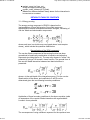
Download DOCK 6.1 User Manual

DOCK 6.1 User Manual
1 of 65
http://dock.compbio.ucsf.edu/DOCK_6/dock6_manual.htm
DOCK 6.1 Users Manual
Authors:
P. Therese Lang (UCSF)
Demetri Moustakas (UCSF/Harvard)
Scott Brozell (The Scripps Research Institute)
Noel Carrascal (SUNY-Stony Brook)
Sudipto Mukherjee (SUNY-Stony Brook)
Scott Pegg (UCSF)
Kaushik Raha (UCSF)
Devleena Shivakumar (The Scripps Research Institute)
Robert Rizzo (SUNY-Stony Brook)
David Case (The Scripps Research Institute)
Brian Shoichet (UCSF)
Irwin Kuntz (UCSF)
Copyright © 2006-2007
Regents of the University of California
All Rights Reserved
Last updated February 9, 2007
Table of Contents
1. Introduction
1.1. General Overview
1.2. What Can DOCK Do for You
1.3. Installation
1.4. What's New in DOCK 6
1.5. Overview of the DOCK Suite of Programs
2. DOCK
9/18/2007 2:30 PM
DOCK 6.1 User Manual
2 of 65
http://dock.compbio.ucsf.edu/DOCK_6/dock6_manual.htm
2.1. Overview
2.2. History
2.3. Command-line Arguments
2.4. The Parameter Parser
2.5. Ligand File Input
2.6. Orienting the Ligand
2.6.1. Sphere Matching
2.6.2. Critical Points
2.6.3. Chemical Matching
2.6.4. Macromolecular Docking
2.7. Ligand Flexibility
2.7.1. Anchor-and-Grow
2.7.2. Identification of Rigid Segments
2.7.3. Manual Specification of Non-rotatable Bonds
2.7.4. Identification of Flexible Layers
2.7.5. Pruning the Conformation Search Tree
2.7.6. Internal Energy Calculation
2.7.7. Time Requirements
2.8. Scoring
2.8.1. Bump Filter
2.8.2. Contact Score
2.8.3. Grid-Based Score
2.8.4. DOCK 3.5 Score
2.8.5. Continuous Score
2.8.6. Zou GB/SA Score
2.8.7. Hawkins GB/SA Score
2.8.8. PB/SA Score
2.8.9. AMBER Score
2.9. Minimization
9/18/2007 2:30 PM
DOCK 6.1 User Manual
3 of 65
http://dock.compbio.ucsf.edu/DOCK_6/dock6_manual.htm
2.10. Parameter Files
2.10.1. Atom Definition Rules
2.10.2. vdw.defn
2.10.3. chem.defn
2.10.4. chem_match.tbl
2.10.5. flex.defn
2.10.6. flex_drive.tbl
2.11. Ligand File Output
2.12. Parallel Processing
3. Accessories
3.1. Grid
3.1.1. Overview
3.1.1. Bump Checking
3.1.2. Contact Scoring
3.1.3. Energy Scoring
3.2. Docktools
3.2.1. Chemgrid
3.2.1. Ligand Desolvation
3.2.2. Occupancy Desolvation
3.2.3. Grid Conversion
3.3. Nchemgrids
3.4. Sphgen
3.4.1. Overview
3.4.2. Critical Points
3.4.3. Chemical Matching
3.4.4. Output
3.5. Showbox
3.6. Showsphere
3.7. Sphere Selector
9/18/2007 2:30 PM
DOCK 6.1 User Manual
4 of 65
http://dock.compbio.ucsf.edu/DOCK_6/dock6_manual.htm
3.8. Antechamber
4. Molecular File Formats
4.1. Tripos MOL2 Format
4.2. PDB Format
5. References
Introduction
RETURN TO TABLE OF CONTENTS
1.1. General Overview
DOCK addresses the problem of "docking" molecules to each other. In general, "docking" is
the identification of the low-energy binding modes of a small molecule, or ligand, within the
active site of a macromolecule, or receptor, whose structure is known. A compound that
interacts strongly with, or binds, a receptor associated with a disease may inhibit its function
and thus act as a drug. Solving the docking problem computationally requires an accurate
representation of the molecular energetics as well as an efficient algorithm to search the
potential binding modes.
Historically, the DOCK algorithm addressed rigid body docking using a geometric matching
algorithm to superimpose the ligand onto a negative image of the binding pocket. Important
features that improved the algorithm's ability to find the lowest-energy binding mode,
including force-field based scoring, on-the-fly optimization, an improved matching algorithm
for rigid body docking and an algorithm for flexible ligand docking, have been added over the
years. For more information on past versions of DOCK, click here.
With the release of DOCK 6, we continue to improve the algorithm's ability to predict binding
poses by adding new features like force-field scoring enhanced by solvation and receptor
flexibility. For more information about the current release of DOCK, click here.
RETURN TO TABLE OF CONTENTS
1.2. What Can DOCK Do for You
We and others have used DOCK for the following applications:
predict binding modes of small molecule-protein complexes
search databases of ligands for compounds that inhibit enzyme activity
search databases of ligands for compounds that bind a particular protein
search databases of ligands for compounds that bind nucleic acid targets
examine possible binding orientations of protein-protein and protein-DNA complexes
help guide synthetic efforts by examining small molecules that are computationally
derivatized
many more...
RETURN TO TABLE OF CONTENTS
9/18/2007 2:30 PM
DOCK 6.1 User Manual
5 of 65
http://dock.compbio.ucsf.edu/DOCK_6/dock6_manual.htm
1.3. Installation
NOTE FOR WINDOWS USERS: DOCK and its accessories must be run using a Linux-like
environment like Cygwin ( http://www.cygwin.com/ ). When you install your emulator, make
sure to also install compilers, unix shells, and perl ( Devel for Cygwin ). All steps below
should be performed using Cygwin or another Windows-based Linux emulator.
(1) Decompress and extract folders using the following commands:
[user@dock ~] tar -zxvf dock.6.1.tar.gz
(2) Enter the installation directory
[user@dock ~] cd dock6/install
(3) Configure the Makefile for the appropriate operating system
[user@dock ~] ./configure [configuration file]
AUTHOR: Scott Brozell
USAGE: configure [-help] [configuration file]
OPTIONS
-help #emit the usage statement
configuration file #input file containing operating system appropriate variables
Configuration Files Target
gnu
gnu-style compiler
gnu.parallel
gnu-style compiler with parallel processing library
capability
gnu.pbsa
gnu-style compiler with PB/SA (ZAP library) capability
gnu.parallel.pbsa
gnu-style compiler with parallel processing library and
PB/SA (ZAP library) capabilities
sgi
sgi-style compiler
sgi.parallel
sgi-style compiler with parallel processing library
capability
DESCRIPTION:
Create the DOCK configuration file, config.h, by copying an existing configuration
file that is selected using the arguments. When invoked without arguments, print
this usage statement and if the configuration file exists then print its creation
stamp. Some configuration files require that environment variables be defined;
these requirements are listed in the files and emitted by configure.
(4) OPTIONAL: Define environment variables.
(i) DOCK with parallel processing functionality requires a Message Passing
Interface (MPI) library. Because of the vagaries of MPI libraries, building parallel
DOCK has more pitfalls than installing the serial version. The MPI library must be
installed and running on the system if the parallel features of DOCK are to be
used.
Currently, the DOCK installation mechanism only directly supports the MPICH2
and MPICH implementations. The MPICH2 library is freely available from
9/18/2007 2:30 PM
DOCK 6.1 User Manual
6 of 65
http://dock.compbio.ucsf.edu/DOCK_6/dock6_manual.htm
Argonne National Labs ( http://www-unix.mcs.anl.gov/mpi/mpich/ ). Once MPI is
installed, define the environment variable MPICH_HOME to the top level MPICH2
directory.
WARNING: The parallel configuration files have been tailored to a typical
MPICH2 build. Linking problems, such as undefined references and cannot find
libbla_bla, can occur due to idiosyncrasies in the MPI installation. One corrective
approach is to use manual linking; add to the LIBS definition in config.h the link
flags (-L and -l) from the command: $MPICH_HOME/mpicc -show; in general, the
LIBS should contain those link flags in the same order.
(ii) DOCK with PB/SA scoring requires the OpenEye ZAP library. The ZAP library
can be obtained from OpenEye (http://www.eyesopen.com/). Once ZAP is
installed, define the environment variable ZAP_HOME to the directory that
contains the ZAP library.
(5) Build the desired DOCK executable(s) via one of the following commands:
[user@dock ~] make all # builds all the DOCK programs
[user@dock ~] make dock # builds only the dock program
[user@dock ~] make utils # builds only the accessory programs
(6) Test the built executable(s) via this sequence of commands:
[user@dock ~] cd test
[user@dock ~] make clean
[user@dock ~] make test
This directory contains the DOCK quality control (QC) suite. It produces pass/fail
results via fast regression tests. The suite should complete in less than ten
minutes; un-passed tests should be examined to determine their significance.
If failures occur then examine the outputs via the command:
[user@dock ~] make check
NOTE: Some failures are not significant. For example, differences in the tails of
floating point numbers may not be significant. The sources of such differences are
frequently platform dependencies from computer hardware, operating systems,
and compilers that impact arithmetic precision and random number generators.
We are working on increasing DOCK's resilience to these issues. For now, apply
common sense and good judgment to determine the significance of a possible
failure.
If you have problems with any of the steps above, please contact us at
[email protected] with a full description of your problem.
RETURN TO TABLE OF CONTENTS
1.4. What's New in DOCK 6
Version 6.0
The new features of DOCK 6 include:
additional scoring options during minimization; DOCK 3.5 scoring-including Delphi
electrostatics, ligand conformational entropy corrections, ligand desolvation, receptor
desolvation; Hawkins-Cramer-Truhlar GB/SA solvation scoring with optional salt screening;
PB/SA solvation scoring; AMBER scoring-including receptor flexibility; the full AMBER
9/18/2007 2:30 PM
DOCK 6.1 User Manual
7 of 65
http://dock.compbio.ucsf.edu/DOCK_6/dock6_manual.htm
molecular mechanics scoring function with implicit solvent; conjugate gradient minimization
and molecular dynamics simulation capabilities.
Version 6.1
The newly added features for the incremental release of DOCK 6 include a new pruning
algorithm during the anchor-and-grow algorithm, a distance-based movable region and a
mildly performance optimized nothing movable region for AMBER score, cleaner output and
more complete output files for AMBER score, the ability to perform ranking and/or clustering
on ligands between primary and secondary scoring, and more dynamic output when
secondary scoring is employed.
RETURN TO TABLE OF CONTENTS
1.5. Overview of the DOCK Suite of Programs
1.5.1. Programs
The relationship between the main programs in the dock suite is depicted in Figure 1. These
routines will be described below.
Main programs in DOCK suite
The program sphgen
identifies the active site, and other sites of interest, and generates the sphere centers that fill
the site. It has been described in the original paper (Kuntz, et al. J. Mol. Biol. 1982). The
program grid generates the scoring grids (Shoichet, et al. J. Comp. Chem. 1992 and Meng,
et al. J. Comp. Chem. 1992). Within the DOCK suite of programs, the program DOCK
matches spheres (generated by sphgen) with ligand atoms and uses scoring grids (from grid)
to evaluate ligand orientations (Kuntz, et al. J. Mol. Biol. 1982 and Shoichet, et al. J. Comp.
Chem. 1992). Program DOCK also minimizes energy based scores (Meng, et al. Proteins.
1993).
1.5.2. General Concepts
The DOCK suite of programs is designed to find favorable orientations of a ligand in a
“receptor.” It can be subdivided into
(i) those programs related directly to docking of ligands and
(ii) accessory programs.
We limit the discussion in this section to only those programs and methods related to docking
a ligand in a receptor. A typical receptor might be an enzyme with a well-defined active site,
though any macromolecule may be used (e.g. a structural protein, a nucleic acid strand, a
9/18/2007 2:30 PM
DOCK 6.1 User Manual
8 of 65
http://dock.compbio.ucsf.edu/DOCK_6/dock6_manual.htm
“true” receptor). We’ll use an enzyme as an example in the rest of this discussion.
The starting point of all docking calculations is generally the crystal or NMR structure of an
enzyme from an enzyme-ligand complex. The ligand structure may be taken from the crystal
structure of the enzyme-ligand complex or from a database of compounds, such as the ZINC
database (Irwin, et. al. J. Chem. Inf. Model. 2005). The primary consideration in the design of
our docking programs has been to develop methods which are both rapid and reasonably
accurate. These programs can be separated functionally into roughly two parts, each
somewhat independent of the other:
(i) Routines which determine the orientation of a ligand relative to the receptor
and
(ii) Routines which evaluate (score) a ligand orientation.
There is a lot of flexibility. You can generate orientations outside of DOCK and score them
with the DOCK evaluation functions. Alternatively, you can develop your own scoring routines
to replace the functions supplied with DOCK.
The ligand orientation in a receptor site is broken down into a series of steps, in different
programs. First, a potential site of interest on the receptor is identified. (Often, the active site
is the site of interest and is known a priori.) Within this site, points are identified where ligand
atoms may be located. A routine from the DOCK suite of programs identifies these points,
called sphere centers, by generating a set of overlapping spheres which fill the site. Rather
than using DOCK to generate these sphere centers, important positions within the active site
may be identified by some other mechanism and used by DOCK as sphere centers. For
example, the positions of atoms from the bound ligand may be used as these sphere centers.
Or, a grid may be generated within the site and each grid point may be considered as a
sphere center. Our sphere centers, however, attempt to capture shape characteristics of the
active site (or site of interest) with a minimum number of points and without the bias of
previously known ligand binding modes.
To orient a ligand within the active site, some of the sphere centers are “matched” with ligand
atoms. That is, a sphere center is “paired” with an ligand atom. Many sets of these
atom-sphere pairs are generated, each set containing only a small number of sphere-atom
pairs. In order to limit the number of possible sets of atom-sphere pairs, a longest distance
heuristic is used; (long) inter-sphere distances are roughly equal to the corresponding (long)
inter-atomic ligand distances. A set of atom-sphere pairs is used to calculate an orientation of
the ligand within the site of interest. The set of sphere-atom pairs which are used to generate
an orientation is often referred to as a match. The translation vector and rotation matrix which
minimizes the rmsd of (transformed) ligand atoms and matching sphere centers of the
sphere-atom set are calculated and used to orient the entire ligand within the active site.
The orientation of the ligand is evaluated with a shape scoring function and/or a function
approximating the ligand-enzyme binding energy. Most evaluations are done on (scoring)
grids in order to minimize the overall computational time. At each grid point, the enzyme
contributions to the score are stored. That is, receptor contributions to the score, potentially
repetitive and time consuming, are calculated only once; the appropriate terms are then
simply fetched from memory.
The ligand-enzyme binding energy is taken to be approximately the sum of the van der Waal
attractive, van der Waal dispersive, and Coulombic electrostatic energies. Approximations
are made to the usual molecular mechanics attractive and dispersive terms for use on a grid.
To generate the energy score, the ligand atom terms are combined with the receptor terms
from the nearest grid point, or combined with receptor terms from a “virtual” grid point with
interpolated receptor values. The score is the sum of over all ligand atoms for these
combined terms. In this case, the energy score is determined by both ligand atom types and
9/18/2007 2:30 PM
DOCK 6.1 User Manual
9 of 65
http://dock.compbio.ucsf.edu/DOCK_6/dock6_manual.htm
ligand atom positions on the energy grids.
As a final step, in the energy scoring scheme, the orientation of the ligand may be varied
slightly to minimize the energy score. That is, after the initial orientation and evaluation
(scoring) of the ligand, a simplex minimization is used to locate the nearest local energy
minimum. The sphere centers themselves are simply approximations to possible atom
locations; the orientations generated by the sphere-atom pairing, although reasonable, may
not be minimal in energy.
1.5.3. Specific Concepts
(A) Sphere Centers
Spheres are generated to fill the target site. The sphere centers are putative
ligand atom positions. Their use is an attempt to limit the enormous number of
possible orientations within the active site. Like ligand atoms, these spheres touch
the surface of the molecule and do not intersect the molecule. The spheres are
allowed to intersect other spheres; i.e. they have volumes which overlap. Each
sphere is represented by the coordinates of its center and its radius. Only the
coordinates of the sphere centers are used to orient ligands within the active site
(see above). Sphere radii are used in clustering.
The number of orientations of the ligand in free space is vast. The number of
orientations possible from all sets of sphere-atom pairings is smaller but still large
and cannot be generated and evaluated (scored) in a reasonable length of time.
Consequently, various filters are used to eliminate from consideration, before
evaluation, sets of sphere-atoms pairs, which will generate poorly scoring
orientations. That is, only a small subset of the number of possible ligand
orientations are actually generated and scored. The distance tolerance is one
filter. Sphere “coloring” and identification of “critical” spheres are other filters.
Sphere-sphere distances are compared to atom-atom distances. Sets of
sphere-atom pairs are generated in the following manner: sphere i is paired with
atom I if and only if for every sphere j in the set and for every atom J in the set,
where dij is the distance between sphere i and sphere j, dIJ is the distance
between atom I and atom J, and epsilon is a somewhat small user-defined value.
(B) Chemical Matching
DOCK spheres are generated without regard to the chemical properties of the
nearby receptor atoms. Sphere “chemical matching” or “coloring” associates a
chemical property to spheres and a sphere of one “color” can only be matched
with a ligand atom of complementary color. These chemical properties may be
things such as “hydrogen-bond donor,” “hydrogen-bond acceptor,” “hydrophobe,”
“electro-positive,” “electro-negative,” “neutral,” etc. Neither the colors themselves,
nor the complementarity of the colors, are determined by the DOCK suite of
programs; DOCK simply uses these labels. With the inclusion of coloring, only
ligand atoms with the appropriate chemical properties are matched to the
complementary colored spheres. It is probably more likely, then, that the
orientation generated will produce a favorable score. Conversely, by excluding
colored spheres from pairing with certain ligand atoms, the number of (probably)
unfavorable orientations which are generated and evaluated can be reduced.
9/18/2007 2:30 PM
DOCK 6.1 User Manual
10 of 65
http://dock.compbio.ucsf.edu/DOCK_6/dock6_manual.htm
Note that requiring complementarity in matching does not mean that all ligand
atoms will lie in chemically complementary regions of the enzyme. Rather, only
those ligand atoms, when paired with a colored sphere which is part of the
sphere-atom match, will be guaranteed to be in the chemically complementary
region of the enzyme (provided chirality of the spheres is the same as that of the
matching ligand atoms).
(C) Critical Points
The "critical point" filter requires that certain spheres be part of the set of
sphere-atom pairs used to orient the ligand (DesJarlais, et al. J. Comput-Aided
Molec. Design. 1994). Designating spheres as critical points forces the ligand to
have at least one atom in that area of the enzyme, where that sphere is located.
This filter may be useful, for example, when it is known that a ligand must occupy
a particular area of an active site. This filter removes from consideration any
orientation that does not guarantee at least one ligand atom in critical areas of the
enzyme (provided chirality of the spheres is the same as that of the matching
ligand atom).
(D) Bump Filter
After a ligand is oriented within the active site, the orientation is evaluated. In an
attempt to reduce the total computational time, after the ligand is oriented in the
site, it is possible to first check whether or not ligand atoms occupy space already
occupied by the receptor. If too many of such “bumps” are found, then the ligand
is likely to intersect the receptor even after minimization; consequently, the ligand
orientation is discarded before evaluation.
RETURN TO TABLE OF CONTENTS
DOCK
RETURN TO TABLE OF CONTENTS
2.1. Overview
This section is intended as a reference manual for the features of the DOCK Suite of
Programs. It is intended to give an overview of the ideas which form the basis of the DOCK
suite of programs and to detail the available user parameters. It is not intended to be a
substitute for all the papers written on DOCK.
In general, this document is geared towards the experienced user and introduces new
features and concepts in version 6. If you are new to DOCK, we strongly recommend you
look at the tutorials on the DOCK web site at
http://dock.compbio.ucsf.edu/DOCK_6/index.htm, which go into much greater practical detail.
RETURN TO TABLE OF CONTENTS
2.2. History
Version 1.0/1.1
Authors: Robert Sheridan, Renee DesJarlais, Irwin Kuntz
9/18/2007 2:30 PM
DOCK 6.1 User Manual
11 of 65
http://dock.compbio.ucsf.edu/DOCK_6/dock6_manual.htm
The program DOCK is an automatic procedure for docking a molecule into a receptor site.
The receptor site is characterized by centers, which may come from SPHGEN or any other
source. The molecule being docked is characterized by ligand centers, which may be its
non-hydrogen atoms or volume-filling spheres calculated in SPHGEN. The ligand centers
and receptor centers are matched based on comparison of ligand-center/ligand-center and
receptor-center/receptor-center distances. Sets of ligand centers match sets of receptor
centers if all the internal distances match, within a value of distance_tolerance.
Ligand-receptor pairs are added to the set until at least nodes_minimum pairs have been
found. At least three pairs must be found to uniquely determine a rotation/translation matrix
that will orient the ligand in the receptor site. A least-squares fitting procedure is used (Ferro,
et al Act. Cryst. A. 1977.). Once an orientation has been found, it is evaluated by any of
several scoring functions. DOCK may be used to explore the binding modes of an individual
molecule, or be used to screen a database of molecules to identify potential ligands.
Version 2.0
Authors: Brian Shoichet, Dale Bodian, Irwin Kuntz
DOCK version 2.0 was written to give the user greater control over the thoroughness of the
matching procedure, and thus over the number of orientations found and the CPU time
required (Shoichet, et al. J. Comp. Chem. 1992). In addition, certain algorithmic shortcomings
of earlier versions were overcome. Versions 2.0 and higher are particularly useful for
macromolecular docking (Shoichet, et al J. Mol. Biol. 1991) and applications which demand
detailed exploration of ligand binding modes. In these cases, users are encouraged to run
CLUSTER in conjunction with SPHGEN and DOCK.
To allow for greater control over searches of orientation space, the ligand and receptor
centers are pre-organized according to their internal distances. Starting with any given
center, all the other centers are presorted into “bins” based on their distance to the first
center. All centers are tried in turn as “first” positions, and all the points in a bin which has
been chosen for matching are tried sequentially. Ligand and receptor bins are chosen for
matching when they have the same distance limits from their respective “first” points. The
number of centers in each bin determines how many sets of points in the receptor and the
ligand will ultimately be compared. In general, the wider the bins, the greater the number of
orientations generated. Thus, the thoroughness of the search is under user control.
Version 3.0
Authors: Elaine Meng, Brian Shoichet, Irwin Kuntz
Version 3.0 retained the matching features of version 2.0, and introduced options for scoring
(Meng, et al. J. Comp. Chem., 1992). Besides the simple contact scores mentioned above,
one can also obtain molecular mechanics interaction energies using grid files calculated by
CHEMGRID (which is now superseded by GRID in version 4.0). More information about the
ligand and receptor molecules is required to perform these higher-level kinds of scoring.
Point charges on the receptor and ligand atoms are needed for electrostatic scoring, and
atom-type information is needed for the van der Waals portion of the force field score. Input
formats (some of them new in version 3.5) are discussed in various parts of the
documentation; one example of a “complete format” (including point charges and atom type
information) is SYBYL MOL2 format. Parameterization of the receptor is discussed in the
documentation for CHEMGRID. In DOCK, ligand parameters are read in along with the
coordinates; input formats are described below. Currently, the options are: contact scoring
only, contact scoring plus Delphi electrostatic scoring, and contact scoring plus force field
scoring. Atom-type information and point charges are not required for contact scoring only.
Version 3.5
9/18/2007 2:30 PM
DOCK 6.1 User Manual
12 of 65
http://dock.compbio.ucsf.edu/DOCK_6/dock6_manual.htm
Authors: Mike Connolly, Daniel Gschwend, Andy Good, Connie Oshiro, Irwin Kuntz
Version 3.5 added several features: score optimization, degeneracy checking, chemical
matching and critical clustering.
Version 4.0
Authors: Todd Ewing, Irwin Kuntz
Version 4.0 was a major rewrite and update of DOCK. A new matching engine was
developed which is more robust, efficient, and easier to use (Ewing, et al. J. Comput. Chem.
1997). Orientational sampling can now be controlled directly by specifying the number of
desired orientations. Additional features include chemical scoring, chemical screening, and
ligand flexibility.
Version 5.0-5.4
Authors: Demetri Moustakas, P. Therese Lang, Scott Pegg, Scott Brozell, Irwin Kuntz
Version 5 was rewritten in C++ in a modular format, which allows for easy implementation of
new scoring functions, sampling methods and analysis tools (Moustakas, et al, 2006).
Additional new features include MPI parallelization, exhaustive orientation searching,
improved conformation searching, GB/SA solvation scoring, and post-screening pose
clustering. (Zou, et al. J. Am. Chem. Soc., 1999)
Version 6.0-6.1
DOCK 6 is an extension of the DOCK 5 code base. It includes the implementation of
Hawkins-Cramer-Truhlar GB/SA solvation scoring with salt screening and PB/SA solvation
scoring through OpenEye's Zap Library. Additional flexibility has been added to scoring
options during minimization. The new code also incorporates DOCK version 3.5.54 scoring
features like Delphi electrostatics, ligand desolvation, and receptor desolvation. Finally,
DOCK 6 introduces new code that allows access to the NAB library of functions such as
receptor flexibility, the full AMBER molecular mechanics scoring function with implicit solvent,
conjugate gradient minimization, and molecular dynamics simulation capabilities.
RETURN TO TABLE OF CONTENTS
2.3. Command-line Arguments
DOCK must be run command line from a standard unix shell. It reads a parameter file
containing field/value pairs using the following command:
USAGE: dock6 -i dock.in [-o dock.out] [-v]
DESCRIPTION:
DOCK may be executed in either interactive or batch mode, depending on whether output is
written to a file. In interactive mode, the user is requested only for parameters relevant to the
particular run and default values are provided. This mode is recommended for the initial
construction of the input file and for short calculations. In batch mode, input parameters are
read in from the input file and all output is written to the output file. This mode is
recommended for long calculations once an input file has been generated interactively.
OPTIONS
-i dock.in #input file containing user-defined parameters
-help #emit the usage statement.
-v #verbosity flag that prints additional information and warnings for scoring functions
9/18/2007 2:30 PM
DOCK 6.1 User Manual
13 of 65
http://dock.compbio.ucsf.edu/DOCK_6/dock6_manual.htm
-o dock.out
#output file containing the parameters used in the calculation, summary information for each
molecule docked, and all warning messages
Interactive mode
USAGE: dock6 -i dock.in
DESCRIPTION:
When launched this way, DOCK will extract all relevant parameters from dock.in
(or any file supplied by the user). If additional parameters are needed (or if the
dock.infile is non-existent or empty), DOCK will request them one at a time from
the user. Reasonable default values are presented. Any parameters supplied by
the user will be automatically appended to the dock.in file. If the user would like to
change any previously entered values, the user can edit in the dock.in file using a
text editor.
Batch mode
USAGE: dock6 -i dock.in -o dock.out
DESCRIPTION:
When launched in this way, DOCK will run in batch mode, extracting all relevant
parameters from dock.in (or any file supplied by the user) and will write out all
output to dock.out(or any file supplied by the user). If any parameters are missing
or incorrect, then execution will halt and an appropriate error message will be
reported in dock.out.
Parallel DOCK
USAGE: mpirun [-machinefile machfile] [-np #_of_proc] dock6.mpi -i dock.in -o
dock.out [-v]
DESCRIPTION:
If you have compiled DOCK for parallel processing (see Installation), DOCK can
be run in parallel. Parallelzation is set up to have a single Master node with the
remaining nodes act as slaves. The Master node performs file processing and
input/output, whereas the slaves perform the actual calculations. If np = 1, the
code defaults to non-MPI behavior. As a result, there will be minimal difference in
performance between 1 and 2 processors. Improved performance will only
become evident with more than 2 nodes.
ADDITIONAL OPTIONS
-machinefile
#simple text file containing the names of the computers (nodes) to be used
-np #
specifies the number of processors which typically is the same as the number of
lines in the machinefile
PB/SA DOCK
USAGE: dock6.pbsa -i dock.in [-o dock.out] [-v]
DESCRIPTION:
If you have compiled DOCK for use with the ZAP library (see Installation), DOCK
can be run using the ZAP PB/SA scoring function.
9/18/2007 2:30 PM
DOCK 6.1 User Manual
14 of 65
http://dock.compbio.ucsf.edu/DOCK_6/dock6_manual.htm
RETURN TO TABLE OF CONTENTS
2.4. The Parameter Parser
In Interactive Mode, dock will dynamically ask the user to enter the appropriate user
parameters. The generic format for the questions is:
parameter_name [default value] (legal values):
The parameter parser requires that the values entered for a parameter exactly match one of
the legal values. For example:
Example A: program_location [Hello_World!] ():
Example B: #_red_balloons [99] ():
Example C: glass_status [half_full] (half_full half_empty):
In Example A, the parameter "program_location" can be assigned any string value, and in
Example B, the parameter "#_red_balloons" can be assigned any integer value. However, in
Example C, the parameter value "glass_status" can only be assigned the strings "half_full" or
"half_empty". If no parameter are assigned by the user, the default value--in brackets--will be
used.
In Batch Mode, all parameters in the dock.in file, must be:
parameter_name value
Note that the parameter_name and corresponding value need to be separated by white
space or a tab.
RETURN TO TABLE OF CONTENTS
2.5. Ligand File Input
Before you can dock a ligand, you will need atom types and charges for every atom in the
ligand. Currently, DOCK only reads the Tripos MOL2 format. For a single ligand (or several
ligands), you can use Chimera in combination with antechamber to prepare a MOL2 file for
the ligand (see Structure Preparation Tutorial) or various other visualization packages. During
the docking procedure, ligands are read in from a single MOL2 or multi-MOL2 file. Atom and
bond types are assigned using the DOCK 4 atom/bond typing parameter files.
NOTE: The following parameter definitions will use the format below:
parameter_name [default] (value):
#description
In some cases, parameters are only needed (questions will only be asked) if the parameter
above is enforced. These parameters are indicated below by additional indentation.
Molecule Library Parameters
ligand_atom_file [database.mol2] (string):
# The ligand input filename
limit_max_ligands [no] (yes, no):
#Limit the number of ligands to be read in from a library
max_ligands[1000]:
9/18/2007 2:30 PM
DOCK 6.1 User Manual
15 of 65
http://dock.compbio.ucsf.edu/DOCK_6/dock6_manual.htm
#maximum number of ligands that will be read in from a library
skip_molecule [no] (yes, no):
#Skip some number of molecules at the beginning of a library
initial_skip [0] (int):
# The number of molecules to skip over at the beginning of a library
read_mol_solvation [no] (yes, no):
#Flag to read atomic desolvation information from ligand file
calculate_rmsd [no] (yes, no):
#Flag to perform an RMSD calculation between the final molecule pose and its initial
#structure.
use_rmsd_reference_mol [no] (yes, no):
#Specify alternative geometric location for reference structure for RMSD
#calculation
rmsd_reference_filename [ligand_rmsd.mol2] (string):
#File containing alternative geometric location for reference structure for
#RMSD calculation
RETURN TO TABLE OF CONTENTS
2.6. Orienting the Ligand
2.6.1. Sphere Matching
The rigid body orienting code is written as a direct implementation of the
isomorphous subgraph matching method of Crippen and Kuhl (Kuhl, et al. J.
Comput. Chem. 1984). All receptor sphere pairs and atom center pairs are
considered for inclusion in a matching clique. This is more computationally
demanding than the clique matching algorithm implemented in previous versions
that used a distance binning algorithm to restrict the clique search, in which pairs
of spheres and atom centers were binned by distance. Only sphere pairs and
center pairs that were within the same distance bin were considered as potential
matches (Ewing, et al. J. Comput. Chem. 1997) .
The clique matching implementation avoids bin boundaries that prevent some
receptor sphere and ligand atom pairs from matching, and, as a result, it can find
good matches missed by previous versions of DOCK. The rigid body rotation
code has also been corrected to avoid a singularity that occurred if the spheres in
the match lay within the same plane.
There are two types of ligand orientation currently available:
(1) Automated Matching —Specify the number of orientations, and
DOCK will generate matches until enough orientations passing the
bump filter have been formed. Matches are formed best first, with
respect to the difference in the ligand and site point internal distances.
(2) Manual Matching —Specify the distance and node parameters,
and DOCK will generate all the matches which satisfy them. The
number of orientations scored is equal to the total matches minus the
orientations discarded by the user applied filters.
Multiple orientations may be written out for each molecule using the
write_orientations parameter (see Ligand File Output), otherwise only the best
orientation is recorded.
RETURN TO TABLE OF CONTENTS
9/18/2007 2:30 PM
DOCK 6.1 User Manual
16 of 65
http://dock.compbio.ucsf.edu/DOCK_6/dock6_manual.htm
2.6.2. Critical Points
The critical_points feature is used to focus the orientation search into a subsite of
the receptor active site (DesJarlais, et al. J. Comput-Aided Molec. Design. 1994
and Miller, et al J. Comput. Aided Mol. Design. 1994). For example, identifying
molecules that interact with catalytic residues might be of chief interest. Any
number of points may be identified as critical (see Critical Points information on
labeling spheres), and any number of groupings of these points may be identified.
An alternative to using critical points is to discard all site points that are some
distance away from the subsite of interest, while retaining enough site points to
define unique ligand orientations. This feature can be highly effective at reducing
matching by five-fold or more. It is particularly useful to also assign chemical
labels to the critical points to further focus sampling.
RETURN TO TABLE OF CONTENTS
2.6.3. Chemical Matching
The chemical_matching feature is used to incorporate information about the
chemical complementarity of a ligand orientation into the matching process. In
this feature, chemical labels are assigned to site points (see Chemical Matching
for information on labeling spheres) and ligand atoms (see Ligand File Input)
(Kuhl, et al. J. Comput. Chem. 1984). The site point labels are based on the local
receptor environment. The ligand atom labels are based on user-adjustable
chemical functionality rules. These labeling rules are identified with the
chemical_defn_file parameter and reside in an editable file (see chem.defn). A
node in a match will produce an unfavorable interaction if the atom and site point
components have labels which violate a chemical match rule. The chemical
matching rules are identified with the chemical_match_file parameter and reside
in an editable file (see chem_match.tbl). If a match will produce unfavorable
interactions, then the match is discarded. The speed-up from this technique
depends how extensively site points have been labeled and the stringency of the
match rules, but an improvement of two-fold or more can be expected.
RETURN TO TABLE OF CONTENTS
2.6.4. Macromolecular Docking
Although DOCK is typically used to process small ligand molecules, it can be
used to study the interactions of macromolecular eigands. The chief difference in
protocol is that to use the match_receptor_sites procedure for the orientation
search, special ligand centers must be used to represent the ligand. This is
signaled by setting the ligand_centers parameter. The ligand centers may be
constructed by sphgen and must reside in a file identified with the
ligand_center_file parameter. See Shoichet, et al. J. Mol. Biol. 1991 for examples
and discussion of macromolecular docking.
RETURN TO TABLE OF CONTENTS
NOTE: The following parameter definitions will use the format below:
parameter_name [default] (value):
#description
In some cases, parameters are only needed (questions will only be asked) if the parameter
above is enforced. These parameters are indicated below by additional indentation.
9/18/2007 2:30 PM
DOCK 6.1 User Manual
17 of 65
http://dock.compbio.ucsf.edu/DOCK_6/dock6_manual.htm
Orient Ligand Parameters
orient_ligand [yes] (yes, no):
#Flag to orient ligand to spheres
automated_matching [yes] (yes, no):
# Flag to perform automated matching instead of manual matching
(If automated_matching = no, then manual_matching is used)
distance_tolerence [0.25] (float):
#The tolerance in angstroms within which a pair of spheres is considered
equivalent to
#a pair of centers
distance_minimum [2.0] (float):
#The shortest distance allowed between 2 spheres (any sphere pair with a
shorter
#distance is disregarded)
nodes_minimum [3] (int):
#The minimum number of nodes in a clique
nodes_maximum [10] (int):
#The maximum number of nodes in a clique
receptor_site_file [receptor.sph] (string):
# The file containing the receptor spheres
max_orientations [500] (int):
# The maximum number of orientations that will be cycled through
critical_points [no] (yes, no):
#Flag to use critical point sphere labeling to target orientations to particular spheres
chemical_matching [no] (yes, no):
#Flag to use chemical coloring of spheres to match chemical labels on ligand atoms
chem_match_tbl [chem_match.tbl] (string):
#File defining the legal chemical type matches/pairings
use_ligand_spheres [no] (yes/no):
#Flag to enable a sphere file representing ligand heavy atoms to be used to orient the
ligand
#Typically used for macromolecular docking
ligand_sphere_file [ligand.sph] (string):
#The file containing the receptor spheres
RETURN TO TABLE OF CONTENTS
2.7. Ligand Flexibility
2.7.1. Anchor-and-Grow
The process of docking a molecule using the anchor-first strategy is shown in the
Workflow for Anchor-and-Grow Algorithm. First, the largest rigid substructure of
the ligand (anchor) is identified (see Identification of Rigid Segments) and rigidly
oriented in the active site (orientation) by matching its heavy atoms centers to the
receptor sphere centers (see Orienting the Ligand). The anchor orientations are
evaluated and optimized using the scoring function (see Scoring) and the energy
minimizer (see Minimization). The orientations are then ranked according to their
score, spatially clustered by heavy atom root mean squared deviation (RMSD),
and pruned (see Pruning the Conformation Search Tree). Next, the remaining
flexible portion of the ligand (see Identification of Flexible Layers) is built onto the
best anchor orientations within the context of the receptor (grow). It is assumed
that the shape of the binding site will help restrict the sampling of ligand
conformations to those that are most relevant for the receptor geometry.
9/18/2007 2:30 PM
DOCK 6.1 User Manual
18 of 65
http://dock.compbio.ucsf.edu/DOCK_6/dock6_manual.htm
Workflow for Anchor-and-Grow Algorithm
The conformation of a flexible molecule may be searched or relaxed using the flexible_ligand
option. Only the torsion angles are modified, not the bond lengths or angles. Therefore, the
input geometry of the molecule needs to be of good quality. A structure generated by ZINC is
sufficient.
The torsion angle positions reside in an editable file (see flex_drive.tbl on page 111) which is
identified with the flex_drive_file parameter. Internal clashes are detected during the torsion
drive search based on the clash_overlap or internal_energy parameters, which are
independent of scoring function.
RETURN TO TABLE OF CONTENTS
2.7.2. Identification of Rigid Segments
A flexible molecule is treated as a collection of rigid segments. Each segment
contains the largest set of adjacent atoms separated by non-rotatable bonds.
Segments are separated by rotatable bonds.
The first step in segmentation is ring identification.All bonds within molecular rings
are treated as rigid. This classification scheme is a first-order approximation of
9/18/2007 2:30 PM
DOCK 6.1 User Manual
19 of 65
http://dock.compbio.ucsf.edu/DOCK_6/dock6_manual.htm
molecular flexibility, since some amount of flexibility can exist in non-aromatic
rings. To treat such phenomenon as sugar puckering and chair-boat hexane
conformations, the user will need to supply each ring conformation as a separate
input molecule. Additional bonds may be specified as rigid by the user (see
Manual Specification of Non-rotatable Bonds).
Identification of Rigid Anchor and Flexible Bonds
The second step is flexible bond identification. Each flexible bond is associated
with a label defined in an editable file (see flex.defn). The parameter file is
identified with the flex_definition_file parameter. Each label in the file contains a
definition based on the atom types (and chemical environment) of the bonded
atoms. Each label is also flagged as minimizable. Typically, bonds with some
degree of double bond character are excluded from minimization so that planarity
is preserved. Each label is also associated with a set of preferred torsion
positions. The location of each flexible bond is used to partition the molecule into
rigid segments. A segment is the largest local set of atoms that contains only
non-flexible bonds.
RETURN TO TABLE OF CONTENTS
2.7.3. Manual Specification of Non-rotatable Bonds
The user can specify additional bonds to be non-rotatable, to supplement the ring
bonds automatically identified by DOCK. Such a technique would be used to
preserve the conformation of part of the molecule and isolate it from the
conformation search. Non-rotatable bonds are identified in the Tripos MOL2
format file containing the molecule. The bonds are designated as members of a
STATIC BOND SET named RIGID (see Tripos MOL2 Format).
Creation of the RIGID set can be done within Chimera. With the molecule of
interest loaded into Chimera, select the portion of the ligand you would like to
remain rigid. Then select on File > Save MOL2. Make sure the "Write current
selection to @ SETS section of file" is checked and save the file.
Alternatively, the RIGID set can be entered into the MOL2 file by hand. To do this,
go to the end of the MOL2 file. If no sets currently exist, then add a SET identifier
on a new line. It should contain the text "@<TRIPOS>SET". On a new line add
the text "RIGID STATIC BONDS <user> **** Comment". On the next line enter
the number of bonds that will be included in the set, followed by the numerical
identifier of each bond in the set.
RETURN TO TABLE OF CONTENTS
2.7.4. Identification of Flexible Layers
An anchor segment is selected from the rigid segments in an automatic fashion
(see see Manual Specification of Non-rotatable Bonds to override this behavior).
The molecule is divided into segments that overlap at each rotatable bond. The
segment with the largest number of heavy atoms is selected as the anchor. All
segments with more heavy atoms then min_anchor_size are tried separately as
anchors.
9/18/2007 2:30 PM
DOCK 6.1 User Manual
20 of 65
http://dock.compbio.ucsf.edu/DOCK_6/dock6_manual.htm
Identification of Overlapping Segments
When an anchor has been selected, then the molecule is redivided into
non-overlapping segments, which are then arranged concentrically about the
anchor segment. Segments are reattached to the anchor according to the
innermost layer first --and within a layer--the largest segment first.
Layered Non-Overlapping Segments
The anchor is processed separately (either oriented, scored, and/or minimized).
The remaining segments are subsequently re-attached during the conformation
search. The interaction energy between the receptor and the ligand can be
optimized with a simplex minimizer (see Minimization).
RETURN TO TABLE OF CONTENTS
2.7.5. Pruning the Conformation Search Tree
There are now two available methods for pruning available. In the first, the
pruning attempts to retain the best, most diverse configurations using a top-first
pruning method, which proceeds as follows. The configurations are ranked
according to score. The top-ranked configuration is set aside and used as a
reference configuration for the first round of pruning. All remaining configurations
are considered candidates for removal. A root-mean-squared distance (RMSD)
between each candidate and the reference configuration is computed. Each
candidate is then evaluated for removal based on its rank and RMSD using the
inequality shown in Equation 2. If the factor is greater than
number_confs_for_next_growth, as appropriate, the candidate is removed.
9/18/2007 2:30 PM
DOCK 6.1 User Manual
21 of 65
http://dock.compbio.ucsf.edu/DOCK_6/dock6_manual.htm
Based on this factor, a configuration with rank 2 and 0.2 Angstroms RMSD is
comparable to a configuration with rank 20 and 2.0 Angstroms RMSD. The next
best scoring configuration which survives the first pass of removal is then set
aside and used as a reference configuration for the second round of pruning, and
so on. The pruning method biases its search time towards molecules which
sample a more diverse set of binding modes. As the value of
num_anchors_orients_for_growth and number_confs_for_next_growth is
increased, the anchor-first method approaches an exhaustive search.
In the second method, the goal is to bias the sampling toward conformations that
are close to the correct binding mode (as optimized using a test set of
experimentally solved structures). Much as the method above, the algorithm ranks
the generated poses and conformations. Then, all poses that violate a
user-defined score cutoff are removed. To facilitate the speed of the calculation,
the remaining list is additionally pared back to a user-defined length. In this
technique, the sampling is driven towards molecules that sample closer to the
experimentally determined binding site, but results in a significantly less diverse
set of final poses.
RETURN TO TABLE OF CONTENTS
2.7.6. Internal Energy Calculation
During the growth phase of the calculation, an internal energy scoring function
can be used. This function computes the Lennard-Jones and Coulombic energy
between all ligand atom pairs, excluding all 1-2, 1-3, and 1-4 pairs. It reduces the
occurrence of internal clashes during the torsional optimization. This energy is not
included in the final reported score.
RETURN TO TABLE OF CONTENTS
2.7.7. Time Requirements
The time demand grows linearly with the num_anchors_orients_for_growth, the
number_confs_for_next_growth, the number of flexible bonds and the number of
torsion positions per bond, as well as the number of anchor segments explored
for a given molecule. Using the notation in the Workflow for Anchor-and-Grow
Algorithm, the time demand can be expressed as
where the additional terms are:
NA is the number of anchor segments tried per molecule.
NB is the number of rotatable bonds per molecule.
RETURN TO TABLE OF CONTENTS
NOTE: The following parameter definitions will use the format below:
parameter_name [default] (value):
#description
9/18/2007 2:30 PM
DOCK 6.1 User Manual
22 of 65
http://dock.compbio.ucsf.edu/DOCK_6/dock6_manual.htm
In some cases, parameters are only needed (questions will only be asked) if the parameter
above is enforced. These parameters are indicated below by additional indentation.
Flexible Ligand Parameters
flexible_ligand [yes] (yes, no):
#Flag to perform ligand conformational searching
min_anchor_size [40] (int):
#The minimum number of heavy atoms for an anchor segment
pruning_use_clustering [yes] (yes, no):
# Flag to enable clustering during pruning (duplicates previous behavior)
(if pruning_use_clustering = yes)
pruning_max_orients [100] (int):
#The pruning value cutoff for anchor orientations promoted to the conformational
#search (previously num_anchor_orients_for_growth)
pruning_clustering_cutoff [100] (int):
#The maximum number of conformations carried forward in the anchor & grow
search
#(previous num_confs_for_next_growth)
(if pruning_use_clustering = no)
pruning_max_orients [100] (int):
#Maximum number of anchor orientations promoted to the conformational
#search
pruning_orient_score_cutoff [25.0] (float):
#Maximum score for anchor after minimization
pruning_max_conformers [75] (int):
#Maximum number of anchor orientations promoted to the next layer of growth
pruning_conformer_score_cutoff [25.0] (float):
#Maximum score for conformation after minimization
use_internal_energy [yes] (yes,no):
#Flag to add an internal energy term to the score during the conformational search
internal_energy_att_exp [6] (int):
# VDW attractive exponent
internal_energy_rep_exp [12] (int):
#VDW repulsive exponent
internal_energy_dielectric [4.0] (float):
#Dielectric used for electrostatic calculation
use_clash_overlap [no] (yes, no):
#Flag to check for overlapping atom volumes during anchor and grow
clash_overlap [0.5] (float):
#Percent of overlap allowed before a clash is declared
RETURN TO TABLE OF CONTENTS
2.8. Scoring
DOCK uses several types of scoring functions to discriminate among orientations
and molecules. Scoring is requested using the score_molecules parameter. The
scoring functions are implemented with a hierarchical strategy. A master score
class manages all scoring functions that DOCK uses. Any of the DOCK scoring
functions can be selected as the primary and/or the secondary scoring function.
The primary scoring function is used during rigid orienting, anchor-and-grow
steps, and minimization, which typically make many calls to the scoring function.
The secondary scoring function is used in the final minimization, scoring, and
ranking of the molecules.
9/18/2007 2:30 PM
DOCK 6.1 User Manual
23 of 65
http://dock.compbio.ucsf.edu/DOCK_6/dock6_manual.htm
RETURN TO TABLE OF CONTENTS
2.8.1. Bump Filter
Orientations and grow steps may be filtered prior to scoring to discard
those in which the molecule significantly overlaps receptor atoms. This
feature is enabled with the bump_filter flag. At the time of construction
of the bump filter, the amount of atom VDW overlap is defined with the
bump_overlap parameter (see Grid). At the time of bump evaluation
the number of allowed bumps is defined with the max_bump_anchor
and max_bump_growth parameter.
NOTE: The following parameter definitions will use the format below:
parameter_name [default] (value):
#description
In some cases, parameters are only needed (questions will only be
asked) if the parameter above is enforced. These parameters are
indicated below by additional indentation.
Bump Filter Parameters
bump_filter [yes] (yes, no):
#Flag to perform bump filtering
bump_grid_prefix [grid] (string):
#The prefix to the grid file containing the desired bump grid
max_bumps_anchor [12] (int):
#The maximum allowed number of bumps for a molecule to pass
#the filter
max_bumps_growth [12] (int):
#The maximum allowed number of bumps for a molecule to pass
#the filter
RETURN TO TABLE OF CONTENTS
2.8.2. Contact Score
The contact score is a simple summation of the number of heavy atom
contacts between the ligand and receptor. At the time of construction
of the contact scoring grid, the distance threshold defining a contact is
set with the contact_cutoff_distance (see Grid). Atom VDW overlaps
are penalized by checking the bump filter grid, or with the
contact_clash_overlap parameter for the intramolecular score. The
amount of penalty is specified with the contact_clash_penalty
parameter.
The contact score provides a simple assessment of shape
complementarity. It can be useful for evaluating primarily non-polar
interactions.
NOTE: The following parameter definitions will use the format below:
parameter_name [default] (value):
#description
In some cases, parameters are only needed (questions will only be
9/18/2007 2:30 PM
DOCK 6.1 User Manual
24 of 65
http://dock.compbio.ucsf.edu/DOCK_6/dock6_manual.htm
asked) if the parameter above is enforced. These parameters are
indicated below by additional indentation.
Contact Score Parameters
contact_score_primary [no] (yes, no):
#Flag to perform contact scoring as the primary scoring function
contact_score_secondary [no] (yes, no):
#Flag to perform contact scoring as the secondary scoring
function
contact_score_cutoff_distance [4.5] (float):
#The distance threshold defining a contact
contact_score_clash_overlap [0.75] (float):
#Contact definition for use with intramolecular scoring
contact_score_clash_penalty [50] (float):
#The penalty for each contact overlap made
contact_score_grid_prefix [grid] (string):
#The prefix to the grid files containing the desired contact
#grid
RETURN TO TABLE OF CONTENTS
2.8.3. Grid-Based Score
The grid-based score is based on the non-bonded terms of the
molecular mechanic force field (see Grid for more background).
NOTE: The following parameter definitions will use the format below:
parameter_name [default] (value):
#description
In some cases, parameters are only needed (questions will only be
asked) if the parameter above is enforced. These parameters are
indicated below by additional indentation.
Grid Score Parameters
grid_score_primary [yes] (yes, no):
# Flag to perform grid-based energy scoring as the primary
scoring
#function
grid_score_secondary [yes] (yes, no):
# Flag to perform grid-based energy scoring as the secondary
#scoring function
grid_score_rep_rad_scale [1] (float):
#Scalar multiplier of the radii for the repulsive portion of the
#VDW energy component ONLY
grid_score_vdw_scale [1] (float):
# Scalar multiplier of the VDW energy component
(if grid_score_vdw_scale = 0)
grid_score_turn_off_vdw [yes] (yes, no):
#Flag to turn of vdw portion of scoring function
grid_score_es_scale [1] (float):
# The prefix to the grid files containing the desired energy
#grid
9/18/2007 2:30 PM
DOCK 6.1 User Manual
25 of 65
http://dock.compbio.ucsf.edu/DOCK_6/dock6_manual.htm
(if grid_score_es_scale = 0)
grid_score_turn_off_es [yes] (yes, no):
#Flag to turn of es portion of scoring function
grid_score_grid_prefix [grid] (string):
#The prefix to the grid files containing the desired nrg grid
RETURN TO TABLE OF CONTENTS
2.8.4. DOCK3.5 Score
DOCK3.5 score is a variant of Grid-based scoring (see Grid).
DOCK3.5 score function calculates ligand desolvation in addition to
steric and electrostatic interactions between the ligand and receptor.
The electrostatic interactions between the ligand and the protein is
calculated from a electrostatic potential (ESP) map. The ESP map
should be calculated using finite difference Poisson-Boltzmann
equation (PBE) as implemented in the program DelPhi. We provide
scripts for the calculation, however DelPhi is not distributed by us.
In the DOCK scoring hierarchy DOCK3.5 Score follows GridScore and
can be used both as the primary and the secondary scoring function.
NOTE: The following parameter definitions will use the format below:
parameter_name [default] (value):
#description
In some cases, parameters are only needed (questions will only be
asked) if the parameter above is enforced. These parameters are
indicated below by additional indentation.
DOCK3.5 Score Parameters
dock3.5_score_primary [no] (yes, no):
#Flag to perform dock3.5 scoring as the primary scoring function
dock3.5_score_secondary [no] #Flag to perform dock3.5 scoring
as the secondary scoring
#function
dock3.5_vdw_score [yes] (yes, no):
#Calculate steric interaction from dock3.5 score
dock3.5_grd_prefix [chem52] (string):
#Default prefix for files containing dock3.5 grids
dock3.5_electrostatic_score [yes] (yes, no):
#Calculate electrostatic interaction from ESP grid
calculated using DelPhi
dock3.5_ligand_internal_energy [no] (yes, no):
#Flag to add ligand internal energy to the scoring function
dock3.5_ligand_desolvation_score [volume] (volume, total,
no):
#Calculate total or volume based ligand desolvation from
solvation
#grids
dock3.5_solvent_occlusion_file [solvmap] (string):
#Occluded solvent grid of the receptor
dock3.5_redistribute_positive_desolvation [no] (yes,
no):
9/18/2007 2:30 PM
DOCK 6.1 User Manual
26 of 65
http://dock.compbio.ucsf.edu/DOCK_6/dock6_manual.htm
#positive partial atomic desolvation penalties are
distributed
dock3.5_write_atomic_energy_contrib[no] (yes, no):
#write contribution from each atom to total score
dock3.5_score_vdw_scale [1.0] (float):
#Scalar multiplier of VDW energy component
dock3.5_score_es_scale [1.0] (float):
#Scalar multiplier of electrostatic energy component
RETURN TO TABLE OF CONTENTS
2.8.5. Continuous Score
Continuous scoring may be used to evaluate a ligand:receptor
complex without the investment of a grid calculation, or to perform a
more detailed calculation without the numerical approximation of the
grid. When continuous scoring is requested, then score parameters
normally supplied to grid, must also be supplied to DOCK. It is left to
the user to make sure consistent values are supplied to both
programs.
The distance dependence of the Lennard-Jones function is set with
the cont_score_att_exp and cont_score_rep_exp parameters.
Typically a 6-12 potential is used, but it can be softened up by using a
6-8 or 6-9 potential. Regardless of the exponent values selected, the
same radii and well-depths are used. The distance dependence of the
Coulombic function is set with the distance_dielectric parameter. The
dielectric constant is adjusted with the cont_score_dielectric
parameter.
NOTE: The following parameter definitions will use the format below:
parameter_name [default] (value):
#description
In some cases, parameters are only needed (questions will only be
asked) if the parameter above is enforced. These parameters are
indicated below by additional indentation.
Continuous Score Parameters
continuous_score_primary [no] (yes, no):
#Flag to perform continuous non-grid based scoring as the
primary
#scoring function
continuous_score_secondary [no] (yes, no):
#Flag to perform continuous non-grid based scoring as the
#secondary scoring function
cont_score_rec_filename [receptor.mol2] (string):
#File that contains receptor coordinates
cont_score_att_exp [6] (int):
#VDW Lennard-Jones potential attractive exponent
cont_score_rep_ex [12] (int):
#VDW Lennard-Jones potential repulsive exponent
cont_score_dielectric [4.0] (float):
#Dielectric constant for electrostatic term
9/18/2007 2:30 PM
DOCK 6.1 User Manual
27 of 65
http://dock.compbio.ucsf.edu/DOCK_6/dock6_manual.htm
cont_score_vdw_scale [1] (float):
#Scalar multiplier of vdw energy component
(if cont_score_vdw_scale = 0)
cont_score_turn_off_vdw [yes] (yes, no):
#Flag to turn of vdw portion of scoring function
cont_score_es_scale [1] (float):
#Scalar multiplier of electrostatic energy component
(if cont_score_es_scale = 0)
cont_score_turn_off_es [yes] (yes, no):
#Flag to turn of es portion of scoring function
RETURN TO TABLE OF CONTENTS
2.8.6. Zou GB/SA Score
The Zou GB/SA scoring function is a fast algorithm, the pairwise free
energy model, for ligand binding affinity calculations. Specifically, a
pairwise descreening approximation (Hawkins, et al. Chem. Phys. Lett.
1995) is used in calculations of the electrostatic energy contribution.
The algorithm also includes a procedure to account for the low
dielectric region that might form between the ligand and the receptor
during docking processes. It has been tested to obtain similar results
compared with the grid-based free energy model but with much less
computation efforts.
For more information on the scoring function and specifics of the
implementation, see Liu, et al J. Phys. Chem. B. 2004.
Zou GB/SA Score Parameters
gbsa_zou_score_primary [no] (yes, no):
#Flag to perform Zou GB/SA scoring as the primary scoring
#function
gbsa_zou_score_secondary [no] (yes, no):
#Flag to perform Zou GB/SA scoring as the secondary scoring
#function
gbsa_zou_gb_grid_prefix [gb_grid] (string):
# The path to the pairwise GB grids
gbsa_zou_sa_grid_prefix [sa_grid] (string):
#The path to the SA grids
gbsa_zou_vdw_grid_prefix [grid] (string):
#The path to the nrg grids, used for the vdw portion of the
GB/SA calculation
gbsa_zou_screen_file [screen.in] (string):
# GB parameter file for electrostatic screening. Its located
in the parameters dir by default
gbsa_zou_solvent_dielectric [78.300003] (float):
# The value for the solvent dielectric
RETURN TO TABLE OF CONTENTS
2.8.7. Hawkins GB/SA Score
The Hawkins GB/SA score is an implementation of the Molecular
Mechanics Generalized Born Surface Area (MM-GBSA) method
originally described by (Srinivasan, et al. J. Am. Chem. Soc. 1998) and
9/18/2007 2:30 PM
DOCK 6.1 User Manual
28 of 65
http://dock.compbio.ucsf.edu/DOCK_6/dock6_manual.htm
reviewed by (Kollman, et al. Acc. Chem. Res. 2000). This particular
implementation of MM-GBSA uses the pairwise GB solvation model
reported by Hawkins, Cramer and Truhlar (Hawkins, et al. Chem.
Phys. Lett. 1995 , Hawkins, et al. J. Phys. Chem. 1996) with
parameters described by Tsui and Case (Tsui, et al. Biopolymers
2001). Solvent Accessible Surface Areas (SA) are computed using a
C++ implementation of the Amber8 "icosahedra" algorithm.
The total interaction between the ligand and receptor are represented
by unscaled Coulombic and Lennard jones energy terms (MM) plus
the change (delta) in solvation (GBSA) where deltaGBSA = GBSA
complex - (GBSA receptor + GBSA ligand). For any given species
GBSA = Gpolar ( GB energy) + Gnonpolar (SA*0.00542 + 0.92). Note
that if inner and outer dielectric constants are set to 1 (gas-phase) and
80 (water-phase), then GBSA terms are formally equivalent to free
energies of hydration that can be directly compared with experimental
data and useful for evaluating the accuracy of different partial charge
models (Rizzo et al. J. Chem. Theory. Comput. 2006).
The Hawkins GB/SA score was intended to be used for "single-point"
calculations and the current implementation is quite slow if energy
minimization is performed at the same time. However, an energy
minimization is highly recommended prior to GBSA single-point
calculations given that scores can be very sensitive to receptor-ligand
geometry. Use of the -v flag will yield separate GBSA terms for each
species (complex, receptor, and ligand) and also include raw
icosahedra SA values in units of angstroms squared. This scoring
method requires that the vdw_AMBER_parm99.defn file be specified
which contains GB radii and scale parameters for each atom type.
NOTE: The following parameter definitions will use the format below:
parameter_name [default] (value):
#description
In some cases, parameters are only needed (questions will only be
asked) if the parameter above is enforced. These parameters are
indicated below by additional indentation.
Hawkins GB/SA Score Parameters
gbsa_hawkins_score_primary [no] (yes, no):
#Flag to perform Hawkins GB/SA scoring as the primary scoring
#function
gbsa_hawkins_score_secondary [no] (yes, no):
#Flag to perform Hawkins GB/SA scoring as the secondary
scoring
#function
gbsa_hawkins_score_rec_filename [receptor.mol2] (string):
#File that contains receptor coordinates
gbsa_hawkins_score_solvent_dielectric [78.5] (float):
#Dielectric constant for solvent
gbsa_hawkins_score_salt_conc(M) [0.0] (float):
#Salt concentration for solvent at Molar concentration
gbsa_hawkins_score_gb_offset [0.09] (float):
9/18/2007 2:30 PM
DOCK 6.1 User Manual
29 of 65
http://dock.compbio.ucsf.edu/DOCK_6/dock6_manual.htm
#GB radius offset
gbsa_hawkins_score_cont_vdw_and_es [yes] (yes, no):
#Flag to determine whether vdw and es values will be
#calculated continuously or from a grid
(if gbsa_hawkins_score_cont_vdw_and_es = yes)
gbsa_hawkins_score_vdw_att_exp [6] (int):
#VDW Lennard-Jones potential attractive exponent
gbsa_hawkins_score_vdw_att_exp [12] (int):
#VDW Lennard-Jones potential repulsive exponent
(if gbsa_hawkins_score_cont_vdw_and_es = no)
gbsa_hawkins_score_vdw_att_exp [6] (int):
#VDW Lennard-Jones potential attractive
exponent
gbsa_hawkins_score_vdw_att_exp [12] (int):
#VDW Lennard-Jones potential repulsive
exponent
RETURN TO TABLE OF CONTENTS
2.8.8. PB/SA Score
The PB/SA scoring function is an implementation of the ZAP tool kit
from OpenEye. In order to access the PB/SA function, you must have
the ZAP tool kit installed and a valid ZAP license. For more information
on obtaining the tool kit, licensing, and other OpenEye products, go to
the OpenEye web page at www.eyesopen.com
~~~~~~~~~~~~~~~~~~~~~~~~~~~~~~~~~~~~~~~~~~~~~~~~~~~~~~~~~
From the OpenEye Documentation:
"A Smooth Permittivity Function for Poisson-Boltzmann Solvation
Methods", J. Andrew Grant, Barry T. Pickup and Anthony Nicholls, J.
Comp. Chem, Vol 22, No.6, pgs 608-640, April 2001.
ZAP is, at its heart, a Poisson-Boltzmann (PB) solver. The Poisson
equation describes how electrostatic fields change in a medium of
varying dielectric, such as an organic molecule in water. The
Boltzmann bit adds in the effect of mobile charge, e.g. salt. PB is an
effective way to simulate the effects of water in biological systems. It
relies on a charge description of a molecule, the designation of low
(molecular) and high (solvent) dielectric regions and a description of
an ion-accessible volume and produces a grid of electrostatic
potentials. From this, transfer energies between different solvents,
binding energies, pka shifts, pI's, solvent forces, electrostatic
descriptors, solvent dipole moments, surface potentials and dielectric
focusing can all be calculated. As electrostatics is one of the two
principal components of molecular interaction (the other, of course,
being shape), ZAP is OpenEye's attempt to get it right.
ZAP is written in ANSI C and follows a style of object-oriented
programming popularized in the chemical information world by
Daylight. It encapsulates structures and methods by the use of opaque
pointers, or handles. These are integers converted to real pointers in
the interior of the object system, hidden from the user.
9/18/2007 2:30 PM
DOCK 6.1 User Manual
30 of 65
http://dock.compbio.ucsf.edu/DOCK_6/dock6_manual.htm
ZAP is available to most academic and government institutions free of
charge. It comes in the form of a linkable library and a set of
prepackaged binaries compiled for SGI, Linux and Cygwin (NT).
Commercial use requires a license, available at a very reasonable cost
from the nice folks at OpenEye.
~~~~~~~~~~~~~~~~~~~~~~~~~~~~~~~~~~~~~~~~~~~~~~~~~~~~~~~~~
NOTE: The following parameter definitions will use the format below:
parameter_name [default] (value):
#description
In some cases, parameters are only needed (questions will only be
asked) if the parameter above is enforced. These parameters are
indicated below by additional indentation.
PB/SA Score Parameters
pbsa_score_primary [yes] (yes, no):
# Flag to perform pbsa energy scoring as the primary scoring
#function
pbsa_score_secondary [yes] (yes, no):
# Flag to perform pbsa energy scoring as the secondary
#scoring function
pbsa_receptor_filename [receptor.mol2] (string):
# Name of receptor file.
pbsa_interior_dielectric [2.0] (float):
# Value for the dielectric inside the protein
pbsa_exterior_dielectric [78.5] (float):
# Value for the dielectric of the solvent (outside the protein)
pbsa_vdw_grid_prefix [grid] (string):
# The prefix to the grid files containing the VDW values
RETURN TO TABLE OF CONTENTS
2.8.9. AMBER Score
The AMBER score provides a suite of functionality including: AMBER
molecular mechanics, implicit solvation, and molecular dynamics
simulation, receptor flexibility, and conjugate gradient minimization.
The main disadvantages are more complicated input preparation and
increased computational expense.
AMBER score implements molecular mechanics implicit solvent
simulations with the traditional all-atom AMBER force field (Pearlman,
et al. Comp. Phys. Commun. 1995) for protein atoms and the general
AMBER force field (GAFF, Wang, et al. J. Comp. Chem. 2004) for
ligand atoms. The interaction between the ligand and the receptor is
represented by electrostatic and van der Waals energy terms, and the
solvation energy is calculated using a Generalized Born (GB) solvation
model. The user has the option to choose one of the following GB
models: (i) Hawkins, Cramer and Truhlar pairwise GB model with
parameters described by Tsui and Case (gb=1) ( Tsui, et al.
Biopolymers 2001), (ii) Onufriev, Bashford and Case model, GB(OBC)
(gb=2) ( Onufriev, et al. Proteins 2004), and (iii) a modified GB(OBC)
(gb=5) ( Onufriev, et al. Proteins 2004). The surface area term is
9/18/2007 2:30 PM
DOCK 6.1 User Manual
31 of 65
http://dock.compbio.ucsf.edu/DOCK_6/dock6_manual.htm
derived using a fast LCPO algorithm ( Weiser, et al. J. Comp Chem
1999).
The AMBER score is calculated as:
E(Complex) - [ E(Receptor) + E(Ligand) ],
where E(Complex), E(Receptor), and E(Ligand) represent the
energies of the complex, receptor, and ligand, respectively.
The calculation of each of these three energies uses the same
protocol: minimization with a conjugate gradient method is followed by
MD simulation (Langevin molecular dynamics at constant
temperature), another minimization, and a final energy evaluation. The
user can specify the number of pre-MD-minimization cycles, the
number of MD simulation steps, and the number of
post-MD-minimization cycles in the dock input file. During the final
energy evaluation, a surface area term is included. The receptor
energy is determined once. The AMBER score energy protocol is
performed for every ligand and its corresponding complex.
AMBER score enables all or a part of the receptor to be flexible, in
order to reproduce the so-called "induced-fit". The Cartesian
coordinates of atoms that are flexible can be altered during the
AMBER score energy protocol. The Cartesian coordinates of atoms
that are not flexible cannot be altered during the AMBER score energy
protocol. The flexible parts of the receptor-ligand complex are
specified with a movable region dock input file parameter. The
movable region options are ligand, everything, nothing, distance, and
NAB atom expression. For the ligand option, only the ligand is allowed
to move during minimization and MD simulation. For the everything
option, all the atoms in the receptor and the ligand are allowed to
move. No minimization or MD simulation occurs for the nothing option.
This is the only movable region option for which the ligand is not
flexible during the AMBER score energy protocol. Consequently, close
contacts can produce very large energies because the AMBER force
field can be sensitive to the receptor-ligand geometry. However, the
nothing option is the fastest type of AMBER scoring.
The distance movable region option selects residues that are allowed
to move by receptor-ligand distance. If any atom in a receptor residue
is within the dock input file parameter distance cutoff Angstroms of the
ligand then the whole residue is selected. The ligand is represented by
the active site sphere list, and thus the movable receptor residues are
well defined and independent of any particular ligand molecule. The
ligand is always movable. The selected residues are emitted with the
-v verbose flag as a NAB atom expression.
The NAB atom expression movable region option is based on the
program Nucleic Acid Builder (NAB). Every atom in a NAB molecule
has a unique name. This name is composed of the strand name, the
residue number and the atom name. A NAB atom expression is a
character string that contains one or more patterns that match a set of
atom names in a molecule. The dock input file parameter associated
with this option specifies the set of atoms in the receptor that are
movable. All atoms of the ligand are movable. In DOCK a strand name
is in fact a strand sequence number, and in a receptor-ligand complex,
the ligand is always last in the sequence. Thus, a receptor molecule
9/18/2007 2:30 PM
DOCK 6.1 User Manual
32 of 65
http://dock.compbio.ucsf.edu/DOCK_6/dock6_manual.htm
with two strands has strand names of "1" and "2"; in a corresponding
receptor-ligand complex the ligand (which is almost certainly single
stranded) has strand name "3".
NAB atom expressions contain three subexpressions separated by
colons. They represent the strand, residue and atom parts of the atom
expression. Not all three parts are required. An empty part selects all
strands, residues or atoms depending on which parts are empty. Each
subexpression consists of a comma separated list of patterns, or for
the residue part, patterns and/or number ranges. Several atom
expressions may be placed in a single character string by separating
them with the vertical bar. Patterns in atom expressions are similar to
Unix shell expressions. Each pattern is a sequence of one or more
single character patterns and/or stars. The star matches zero or more
occurrences of any single character. Each part of an atom expression
is composed of a comma separated list of limited regular expressions,
or in the case of the residue part, limited regular expressions and/or
ranges. A range is a number or a pair of numbers separated by a
dash. The NAB manual contains more information on atom
expressions.
Here are some examples of NAB atom expressions:
:SER:
#Select all atoms in any residue named SER. All three parts are
present but both the strand and atom parts are empty. The atom
expression :SER selects the same set of atoms.
::C,CA,N,O
#Select all atoms with names C, CA, N or O in all residues in all
strands (typically the peptide backbone).
1:1-10,13:CA,C,N
#Select all atoms named CA,C,N in residues 1-10 and 13 in
strand 1.
::C*[^1]
#The [^1] is an example of a negated character class. It matches
any character in the last position except 1. In this case, it will
match all the atoms starting with C, such as CA, CB, CG2, but
not those ending with 1, such as CD1, CE1.
2::|1:50,100:O*,N*
#Select all atoms in strand 2. Select all atoms whose name
starts with O and N in residue 50, 100 in strand 1. Note that the
vertical bar separates the two strands
4::|2::|1::
#Select strand 4, 2 and 1.
:: or :
#Select all atoms in the molecule.
All the input files, such as the prmtop, frcmod, amber.pdb, etc. should
be generated prior to running the AMBER score. A perl script,
prepare_amber.pl, has been provided for this purpose. The usage of
prepare_amber.pl is
prepare_amber.pl ligand_mol2_file receptor_PDB_file
For example, if lig.mol2 is ligand_mol2_file, and rec.pdb is
receptor_PDB_file, then use: prepare_amber.pl lig.mol2 rec.pdb
The script, prepare_amber.pl, also has the ability to read in a mol2 file
9/18/2007 2:30 PM
DOCK 6.1 User Manual
33 of 65
http://dock.compbio.ucsf.edu/DOCK_6/dock6_manual.htm
containing multiple ligands (usually the output from a previous DOCK
run), and generate AMBER score readable input files.
prepare_amber.pl calls other scripts and programs, such as
antechamber to calculate the AM1-BCC charges for the ligands, and
tleap to assign the parm94 parameter set for protein atoms and the
GAFF parameter set for ligand atoms. See the tutorials for information
on how to use the script to generate the input files. With knowledge of
and experience using AMBER one could create the input files
manually; see the amberize scipts for the gory details. Note that the
ligand_atom_file, which has the extension ".amber_score.mol2", must
have a TRIPOS AMBER_SCORE_ID section.
The AMBER score output in the DOCK output contains energy terms
for each species (complex, receptor, and ligand) such that the sum of
the terms is equal to the score. Use of the DOCK -v verbose flag will
produce detailed energy breakdowns; the formats and definitions of
this information are discussed in the the NAB manual: Nucleic Acid
Builder (NAB). The verbose output is best captured via UNIX shell file
redirection as opposed to the DOCK -o flag.
The AMBER score output in the ligand_outfile_prefix_scored.mol2 file
contains the ligand coordinates extracted from the final structure of the
complex (i.e., the structure after the AMBER score energy protocol is
performed). The ligand charges are from the ligand prmtop file. The
ligand atom types are the normal ones from DOCK and are not the
GAFF atom types used by AMBER score.
The AMBER score uses the following method for emitting all the final
structures in their entirety. The AMBER score will create a file with the
extension ".final_pose.amber.pdb" for every species (receptor, ligands,
and complexes) that contains any movable region (regardless of
whether that region actually exists or actually does move). Thus, for
the distance, everything, and NAB atom expression options of the
movable region, a file for the receptor
(amber_score_receptor_file_prefix.final_pose.amber.pdb) and two for
each ligand,complex pair (AMBER_SCORE_ID.final_pose.amber.pdb,
amber_score_receptor_file_prefix.AMBER_SCORE_ID.final_pose.amber.pdb)
will be created; for the nothing option of the movable region, no files
will be created. In addition, if the -v verbose flag is present then the
AMBER score will create an AMBER restart file with the extension
".final_pose.amber.restart" for every species (receptor, ligands, and
complexes) that contains any movable region (regardless of whether
that region actually exists or actually does move).
Here is some general advice on the AMBER score. Since it is slower
and more complicated than the other scoring functions, one should
proceed carefully when using the AMBER score as the sole primary
score. The most obvious use is to rescore, with the default
amber_score input parameters, the ligands that have been already
scored using one of the faster scoring functions. In general, the input
preparation for AMBER score is more involved than for the other
scores. Effectively, one needs to generate input files for AMBER. In
particular, examine the amberize*.out and *.log files for warnings and
errors. Experience using AMBER will help in understanding and
judging the impact of the messages in these files. Correcting problems
9/18/2007 2:30 PM
DOCK 6.1 User Manual
34 of 65
http://dock.compbio.ucsf.edu/DOCK_6/dock6_manual.htm
may involve substantial effort. See the DOCK Fans mailing list for
specific examples.
NOTE: The following parameter definitions will use the format
below:
parameter_name [default] (value):
#description
In some cases, parameters are only needed (questions will only
be asked) if the parameter above is enforced. These parameters
are indicated below by additional indentation.
AMBER Score Parameters
amber_score_primary [no] (yes, no):
#Flag to perform amber scoring as the primary scoring function.
amber_score_secondary [no] (yes, no):
#Flag to perform amber scoring as the secondary scoring
function. This is temporarily deprecated, and using input
parameter amber_score_secondary causes program termination.
The recommended protocol is to perform two DOCK runs with
the second run specifying amber_score as the primary_score.
amber_score_receptor_file_prefix[rec] (string):
#Prefix of the Receptor. Use the prefix that was used in the
prepare_amber.pl input file preparation step.
amber_score_movable_region [ligand] (distance,
everything, ligand, nab_atom_expression, nothing):
#The region that will be flexible during the scoring protocol.
amber_score_movable_distance_cutoff [3.0] (float):
#All receptor residues within this cutoff in Angstroms
of the ligand will be movable. This is active only for
amber_score_movable_region=distance.
receptor_site_file [receptor.sph] (string):
#The file containing the receptor spheres that define
the active site. This is not specific to amber_score.
This is active for
amber_score_movable_region=distance.
amber_score_movable_atom_expression [::] (string):
#NAB atom expression defining the movable receptor
region. This is active only for
amber_score_movable_region=nab_atom_expression.
amber_score_before_md_minimization_cycles [100] (int):
#Number of conjugate gradient minimization cycles to be
performed before MD.
amber_score_md_steps [3000] (int):
#Number of Molecular Dynamics (MD) steps to be
performed.
amber_score_after_md_minimization_cycles [100] (int):
#Number of conjugate gradient minimization cycles to be
performed after MD.
amber_score_gb_model [5] (int):
#GB model to be used.
amber_score_nonbonded_cutoff [18.0] (float):
#Non-bonded cutoff in Angstroms for the energy
9/18/2007 2:30 PM
DOCK 6.1 User Manual
35 of 65
http://dock.compbio.ucsf.edu/DOCK_6/dock6_manual.htm
calculation.
amber_score_temperature [300.0] (float):
#Temperature at which MD should be performed.
RETURN TO TABLE OF CONTENTS
2.9. Minimization
Score optimization allows the conformation and orientation of a molecule to be adjusted to
improve the score. Although the calculation is expensive, it makes the conformation and
orientation search more efficient because less sampling becomes necessary. Optimization is
activated with the
minimize_ligand parameter. The optimizer currently uses the simplex algorithm, which does
not require evaluation of derivatives (Nelder et al, ComputerJournal, 1964). It does however
depend on a random number generator which makes it sensitive to the initial seed provided
with random_seed parameter. The amount of variance should be small, though. For detailed
calculations, it is recommended that the optimization be repeated with different random
number seeds to check convergence.
The initial step size of the minimizer is specified with the initial_translation, initial_rotation,
and
initial_torsion parameters. The length of minimization may be controlled with the
maximum_iterations parameter. Users can choose to minimize the rigid anchors, minimize
during flexible growth, and minimize the final conformation. The anchor minimization is
always done rigidly; also, if no flexible growth is being done, this step will minimize the entire
molecule. The minimization during the flexible growth is a complete (torsions + rigid)
minimization. When the simplex shrinks enough so that the highest and lowest points are
within the scoring tolerance or if the number of requested minimizer steps is reached, the
minimizer terminates.
RETURN TO TABLE OF CONTENTS
NOTE: The following parameter definitions will use the format below:
parameter_name [default] (value):
#description
In some cases, parameters are only needed (questions will only be asked) if the parameter
above is enforced. These parameters are indicated below by additional indentation.
Score Optimization Parameters
minimize_ligand [yes] (yes, no):
#Flag to perform score optimization
(if flexible_ligand = no)
simplex_max_iterations [50] (int):
#Maximum number of minimization cycles
(if flexible_ligand = yes)
minimize_anchor [yes] (yes, no):
# Flag to perform rigid optimization of the anchor
simplex_anchor_max_iterations [500] (int):
#Maximum number of iterations per cycle per anchor
9/18/2007 2:30 PM
DOCK 6.1 User Manual
36 of 65
http://dock.compbio.ucsf.edu/DOCK_6/dock6_manual.htm
minimize_flexible_growth [yes] (yes, no):
# Flag to perform complete optimization during conformational search
simplex_grow_max_iterations [500] (int):
#Maximum number of iterations per cycle per growth step
use_advanced_simplex_parameters [no] (yes, no):
#Flag to use a simplified set of common minimization parameters for each of the
#minimization steps listed above (see below for list of these options)
(if minimize_ligand = yes)
simplex_final_min [no] (yes, no):
#Flag to perform one more cycle of minimization on each fully grown pose
simplex_final_max_iterations [0] (int):
# Maximum number of iterations for final cycle
simplex_final_min_rep_rad_scale [1] (float):
#Scalar multiplier of the radii for the repulsive portion of the
#VDW energy component ONLY
simplex_final_min_add_internal [no] (yes, no):
#Flag to add ligand internal energy to primary scoring function
(if secondary_score = yes)
simplex_secondary_minimize_pose [yes] (yes, no):
#Flag to perform an additional cycle of minimization using the secondary scoring
#function
use_advanced_secondary_simplex_parameters [no] (yes,no):
#Flag to use a simplified set of common minimization parameters for each of the
#minimization steps listed above (see below for list of these options)
secondary_min_add_internal [no] (yes,no):
#Flag to add ligand internal energy to secondary scoring function
(if minimize = yes)
simplex_random_seed [0] (int):
#Seed for random number generator
Generic Minimizer Parameters
1. if flexible_ligand = no OR use_advanced_simplex_parameters = no, XXX = simplex
2. if use_advanced_simplex_parameters = no AND minimize_anchor = yes, XXX =
simplex_anchor
3. if use_advanced_simplex_parameters = no AND minimize_flexible_growth = yes, XXX
= simplex_growth
4. if use_advanced_simplex_parameters = no AND simplex_final_min = yes, XXX =
simplex_final
5. if simplex_secondary_minimize_pose AND
use_advanced_secondary_simplex_parameters, XXX = simplex_secondary
XXX_max_cycles [1] (int):
#Maximum number of minimization cycles
XXX_score_converge [0.1] (float):
#Exit cycle at when energy converges at cutoff
XXX_cycle_converge [1.0] (float):
# Exit minimization when cycles converge at cutoff
XXX_trans_step [1.0] (float):
#Initial translation step size
9/18/2007 2:30 PM
DOCK 6.1 User Manual
37 of 65
http://dock.compbio.ucsf.edu/DOCK_6/dock6_manual.htm
XXX_rot_step [0.1] (float):
#Initial rotation step size
XXX_tors_step [10.0] (float):
#Initial torsion angle step size
RETURN TO TABLE OF CONTENTS
2.10. Parameter Files
The parameter files contain atom and bond data needed during DOCK calculations. The
definition (*. defn ) files contain atom and bond labeling data. The table (*. tbl ) files contain
additional data for chemical interactions and flexible bond torsion positions. They may be
edited by the user. All the parameter files described below can be found in the "parameter"
directory in the DOCK distribution.
RETURN TO TABLE OF CONTENTS
2.10.1. Atom Definition Rules
The definition files use a consistent atom labeling convention for which
an atom in virtually any chemical environment can be identified. The
specification of adjacent atoms is nested using the elements listed
below:
Each element must be separated by a space.
If more than one adjacent atom is specified, then ALL must be
present (i.e. a boolean AND for rules within a line).
If a label can have multiple definition lines, then any ONE of
them must be satisfied for inclusion (i.e. a boolean OR for rules
on different lines).
Atom Definition Elements
Element Function
atom type Specifies partial or complete atom type. A partial specification is
more general (i.e. "C" versus "C.3"). An asterisk (*) specifies
ANY atom type.
()
Specifies atoms that must be bonded to parent atom.
[]
Specifies atoms that must NOT be bonded to parent atom.
integer
Specifies the number of an atom that must be bonded.
Example Definitions
Example
Explanation
9/18/2007 2:30 PM
DOCK 6.1 User Manual
38 of 65
http://dock.compbio.ucsf.edu/DOCK_6/dock6_manual.htm
C.2 ( 2 O.co2 )
A carboxylate carbon.
.3 [ 3 H ]
Any sp3 hybridized atom that is not attached to
three hydrogens .
C. [ O . ] [ N . [ 2 O.2 ] [ 2 C. ] Any carbon not attached to an oxygen or a
]
nitrogen (unless the nitrogen is a nitro or tertiary
nitrogen).
RETURN TO TABLE OF CONTENTS
2.10.2. vdw.defn
This file contains atom labels and definitions for van der Waals (VDW)
atom typing. The following data types are associated with each atom:
VDW radius, VDW well-depth, flag for heavy atom, and valence. The
VDW radius and VDW well-depth values are used in molecular
mechanics-scoring functions (see Grid). The valence is the value for
the maximum number of atoms that can be attached. The definition is
the Sybyl atom types that should be associated with the atom name. A
label may have multiple definitions.
In the vdw_AMBER_parm99.defn file, there are additional parameters
needed for use with the Hawkins GB/SA scoring function (see
Hawkins GB/SA). Each entry has an additional gbraii and gbscale
parameter.
WARNING: The last entry in the vdw.defn file MUST be Dummy.
Sample Entries
_____________________________________
name Carbon_sp/sp2
atom_model either
radius 1.850
well_depth 0.120
heavy_flag 1
valence 4
definition C
_____________________________________
name Carbon_All_sp3
atom_model all
radius 1.800
well_depth 0.060
heavy_flag 1
valence 4
gbradii 1.70
gbscale 0.72
definition C.3
_____________________________________
9/18/2007 2:30 PM
DOCK 6.1 User Manual
39 of 65
http://dock.compbio.ucsf.edu/DOCK_6/dock6_manual.htm
name Carbon_United_CH3
atom_model united
radius 2.000
well_depth 0.150
heavy_flag 1
valence 4
definition C. ( 3 H )
_____________________________________
RETURN TO TABLE OF CONTENTS
2.10.3. chem.defn
This file contains labels and definitions for chemical labeling. Nothing
outside of addition to a label needs to be assigned to an atom. A label
may have multiple definition lines but the names must match the rules
in the chem_match.tbl file.
Sample Entries
________________________________________________________
name hydrophobic
definition C. [ O. ] [ N . [ 2 O.2 ] [ 2 C. ] ] ( * )
definition N.pl3 ( 3 C. )
definition Cl ( C. )
definition Br ( C. )
definition I ( C. )
definition C.3 [ * ]
________________________________________________________
name donor
definition N. ( H )
definition N.4 [ * ]
________________________________________________________
name acceptor
definition O. [ H ] [ N. ] ( * )
definition O.3 ( 1 * ) [ N. ]
definition O.co2 ( C.2 ( O.co2 ) )
definition N. [ H ] [ N. ] [ O . ] [ 3 . ] ( * )
definition O.2 [ * ]
________________________________________________________
RETURN TO TABLE OF CONTENTS
2.10.4. chem_match.tbl
This file contains the interaction matrix for which chemical labels can
form an interaction in matching. The labels must be identical to labels
in chem.defn. The table flag indicates the beginning of the interaction
table. Compatible labels are identified with a one, otherwise a zero.
Sample File
9/18/2007 2:30 PM
DOCK 6.1 User Manual
40 of 65
http://dock.compbio.ucsf.edu/DOCK_6/dock6_manual.htm
label null
label hydrophobic
label donor
label acceptor
label polar
table
1
11
101
1001
10111
RETURN TO TABLE OF CONTENTS
2.10.5. flex.defn
This file contains labels and definitions for flexible bond identification.
The drive_id field corresponds to a torsion type in the flex_drive.tbl file.
The minimize field is a flag for whether the bond may be minimized.
Two definition lines must be present. Each definition corresponds to
an atom at either end of the bond.
Sample Entries
______________________________________
name sp3-sp3
drive_id 3
minimize 1
definition .3 [ 3 H ] [ 3 O.co2 ]
definition .3 [ 3 H ] [ 3 O.co2 ]
______________________________________
name sp3-sp2
drive_id 4
minimize 1
definition .3 [ 3 H ] [ 3 O.co2 ]
definition .2 [ 2 H ] [ 2 O.co2 ]
______________________________________
name sp2-sp2
drive_id 2
minimize 0
definition .2 [ 2 H ] [ 2 O.co2 ]
definition .2 [ 2 H ] [ 2 O.co2 ]
______________________________________
RETURN TO TABLE OF CONTENTS
2.10.6. flex_drive.tbl
This file contains torsion positions assigned to each rotatable bond
when the flexible docking parameter is used in DOCK. The drive_id
field corresponds to each torsion type in the flex.defn file. The
positions field specifies the number of torsion angles to sample. The
torsions field specifies the angles that are sampled.
Sample Entries
9/18/2007 2:30 PM
DOCK 6.1 User Manual
41 of 65
http://dock.compbio.ucsf.edu/DOCK_6/dock6_manual.htm
______________________________________
drive_id 2
positions 2
torsions 0 180
______________________________________
drive_id 3
positions 3
torsions -60 60 180
______________________________________
drive_id 4
positions 4
torsions -90 0 90 180
______________________________________
RETURN TO TABLE OF CONTENTS
NOTE: The following parameter definitions will use the format below:
parameter_name [default] (value):
#description
In some cases, parameters are only needed (questions will only be asked) if the
parameter above is enforced. These parameters are indicated below by additional
indentation.
Atom Typing Parameters
atom_model [all] (all, united):
#Choice of all atom or united atom models
vdw_defn_file [vdw.defn] (string):
#File containing VDW parameters for atom types
flex_defn_file [flex.defn] (string):
# File containing conformational search parameters
chem_defn_file [chem.defn] (string):
# File containing chemical label definitions
chem_match_tbl [chem_match.tbl] (string):
# File containing rules for chemical matching
RETURN TO TABLE OF CONTENTS
2.11. Ligand File Output
DOCK reports several kinds of information as output which is either written to screen in
interactive mode or written to file in batch mode (see Installation). All input parameters
are echoed into the output. If a parameter is not needed it is not reported in the output.
At the completion of each DOCK run, the number of molecules that were processed
and the total time of the calculation is reported.
The results of each molecule are printed in the outfile as well. Depending on the
combination of user parameters, each molecule entry will contain the number of
anchors used (see Identification of Rigid Segments), the number of orientations that
passed pruning (see Orienting the Ligand), the number of fully grown conformations
that passed pruning (see Pruning the Conformation Search Tree), and a breakdown of
the interaction energy between the ligand and receptor (see Scoring).
Example Molecule Section of Output
9/18/2007 2:30 PM
DOCK 6.1 User Manual
42 of 65
http://dock.compbio.ucsf.edu/DOCK_6/dock6_manual.htm
_______________________________________________
Molecule: C1
Anchors: 1
Orientations: 1
Conformations: 1
Grid Score: -29.223606
vdw: -26.868692
es: -2.254913
In addition to the information printed to the output files, there are several structural
output options. Each structural file name is formed using the ligand_outfile_prefix
parameter. In a typical run, the best scoring pose of each ligand in the library will be
written to a file called outputprefix_scored.mol2. In addition, there are several more
advanced output options:
(1) Users can choose to write out orientations. This will create a file called
outputprefix_orients.mol2. This will write out the molecules after they have
been rigidly oriented and optimized. If anchor & grow is being used, this
option will write out only the anchor fragment. All orientations generated will
be written out, so be careful that the output does not get too huge.
(2) Users can also write out conformers after the final level of optimization.
This will create a file called outputprefix_conformers.mol2. Again, be aware
that the number of molecules in the output file will be equal to the database
size * the # of anchors per molecule * the number of confomations that pass
the final pruning stage * the number of conformers per cycle. This file can
grow quite large, so only use it on single poses or small databases. (NOTE:
If clustering is enabled, all conformations will be written to the
outputprefix_conformers.mol2 file while the clusterheads will be written to
the outputprefix_scored.mol2 file. This seemingly redundant writing is to
ensure that no portion of the analysis is lost if a failure of some kind occurs).
(3) Users can write molecules ranked by score. This will create a file called
outputprefix_ranked.mol2, which writes out the top N molecules from the
database. This option disables the scored molecule output file by default.
If secondary scoring is enabled, all of the above files will be generated for both
primary and secondary scoring. The secondary scoring files will contain both the
original primary score as well as the new secondary score.
NOTE: The following parameter definitions will use the format below:
parameter_name [default] (value):
#description
In some cases, parameters are only needed (questions will only be asked) if the
parameter above is enforced. These parameters are indicated below by additional
indentation.
Ligand File Output
ligand_outfile_prefix [output] (string):
#The prefix that all output files will use
write_orientations [no] (yes, no):
9/18/2007 2:30 PM
DOCK 6.1 User Manual
43 of 65
http://dock.compbio.ucsf.edu/DOCK_6/dock6_manual.htm
#Flag to write all anchor orientations
(if secondary_score = yes)
num_primary_scored_conformers_rescored [1] (int):
#The number of conformations scored and ranked using the primary
score
#to be rescored by the secondary score. Conformations written to
#ligand_outfile_prefix_primary_conformers.mol2
(if num_primary_scored_conformers_rescored > 1):
cluster_primary_conformations [yes] (yes, no):
#Flag to enable clustering of fully minimized conformations
from
#primary score
(if cluster_primary_conformations = yes)
cluster_rmsd_threshold [2.0] (float):
#The cutoff to determine whether conformations
should be
#included in a particular cluster
num_clusterheads_for_rescore [5] (int):
#The number of clusterheads scored using the
primary score
#to be rescored by the secondary score.
Clusterheads
# written to
ligand_outfile_prefix_primary_scored.mol2
num_secondary_scored_conformers_written [1] (int):
#The number of conformations scored and ranked using the
# secondary score. Conformations written to
#ligand_outfile_prefix_secondary_conformers.mol2
rank_primary_ligands [no] (yes, no):
#Flag to enable ranking by primary score over all ligands:
#the set of best scoring poses, one pose per ligand, will be
sorted by
#primary score into descending order. The top poses will be
written to
#file ligand_outfile_prefix_primary_ranked.mol2.
max_primary_ranked [500] (int):
#The maximum number of ligands to be stored in this
_ranked file.
rank_secondary_ligands [no] (yes, no):
#Flag to enable ranking by secondary score over all ligands:
#the set of best scoring poses, one pose per ligand, will be
sorted by
#secondary score into descending order. The top poses will be
written to
#file ligand_outfile_prefix_secondary_ranked.mol2.
max_secondary_ranked [500] (int):
#The maximum number of ligands to be stored in this
_ranked file.
(if secondary_score = no)
num_scored_conformers_written [1] (int):
9/18/2007 2:30 PM
DOCK 6.1 User Manual
44 of 65
http://dock.compbio.ucsf.edu/DOCK_6/dock6_manual.htm
#The number of conformations scored and ranked using the
primary score.
#Conformations written to
#ligand_outfile_prefix_conformers.mol2
(if num_scored_conformers_written > 1):
cluster_conformations [yes] (yes, no):
#Flag to enable clustering of fully minimized conformations
from
#primary score
(if cluster_conformations = yes)
cluster_rmsd_threshold [2.0] (float):
#The cutoff to determine whether conformations should be
#included in a particular cluster
rank_ligands [no] (yes, no):
#Flag to enable ranking by score over all ligands:
#the set of best scoring poses, one pose per ligand, will be
sorted by
#score into descending order. The top poses will be written to
#file ligand_outfile_prefix_ranked.mol2.
max_ranked_ligands [500] (int):
#The maximum number of ligands to be stored in this
_ranked file.
RETURN TO TABLE OF CONTENTS
2.12. Parallel Processing
Parallel processing is fully integrated into the DOCK program. It is set
up to have a single Master node, while the remaining nodes act as
slaves. The Master node performs file processing and input/output,
whereas the slaves perform the actual calculations. If the number of
processors (np) is 1 then the code defaults to the non-MPI behavior.
As a result, there will be a minimal difference in performance between
1 and 2 processors. Improved performance will only become evident
with more than 2 processors. It should be emphasized that the primary
benefit in using DOCK6 in parallel mode is to reduce bookkeeping
tasks associated with manually splitting up a database into multiple
chunks which then must be submitted to different processors
individually. DOCK6 automatically partitions out subsets of a database
to various processors, collates and ranks the final results, and takes
care of all intermediate bookkeeping. Parallel jobs simply require that
the user specify the location of the MPI program used to compile
DOCK6, a machine file listing the names of the nodes, and the total
number of processors to be used. For parallel docking three additional
parameters must be specified: (1) the path of the MPICH2 installation
(i.e /usr/local/mpich2-1.0.4/bin/mpirun), (2) a machine file containing
the names of the computers (nodes) to be used, and (3) the number of
processors which typically is the same as the number of lines in the
machine file. See Commandline Arguments for usage information on
how to run DOCK with parallel processing functionality.
Accessories
9/18/2007 2:30 PM
DOCK 6.1 User Manual
45 of 65
http://dock.compbio.ucsf.edu/DOCK_6/dock6_manual.htm
RETURN TO TABLE OF CONTENTS
3.1. Grid
AUTHOR: Todd Ewing (based on work by Elaine Meng and Brian
Shoichet)
USAGE: grid -i grid.in [-stv] [-o grid.out]
OPTIONS:
- i input_file #Input parameters extracted from input_file, or grid.in if
not specified
-o output_file #Output written to output_file, or grid.out if not specified
-s Input parameters entered interactively
-t Reduced output level
-v Increased output level
DESCRIPTION:
3.1.1. Overview
Grid creates the grid files necessary for rapid score evaluation in
DOCK. Two types of scoring are available: contact and energy
scoring. The scoring grids are stored in binary files ending in *.cnt and
*.nrg respectively. When docking, each scoring function is applied
independent of the others and the results are written to separate
output files. Grid also computes a bump grid which identifies whether a
ligand atom is in severe steric overlap with a receptor atom. The bump
grid is identified with a *.bmp file extension. The binary file containing
the bump grid also stores the size, position and grid spacing of all the
grids.
The grid calculation must be performed prior to docking. The
calculation can take up to 45 minutes, but needs to be done only once
for each receptor site. Grid generation and docking should be
performed on the same platform; because the grid files have a binary
format, copying grid files between machines may produce incorrect
results. Furthermore, binary files should not be modified with text
editors. Since DOCK can perform continuum scoring without a grid,
the grid calculation is not always required. However, for most docking
tasks, such as when multiple binding modes for a molecule or multiple
molecules are considered, it will become more time efficient to
precompute the scoring grids.
NOTE: The following parameter definitions will use the format below:
parameter_name [default] (value):
#description
In some cases, parameters are only needed (questions will only be
asked) if the parameter above is enforced. These parameters are
indicated below by additional indentation.
General Grid Parameters
compute_grids [no] (yes, no):
9/18/2007 2:30 PM
DOCK 6.1 User Manual
46 of 65
http://dock.compbio.ucsf.edu/DOCK_6/dock6_manual.htm
#Flag to compute scoring grids
grid_spacing [0.3] (float):
# The distance between grid points along each axis.
output_molecule [no] (yes, no):
#Flag to write out the coordinates of the receptor into a new,
cleaned-up file. Atoms are
#resorted to put all residue atoms together
receptor_out_file [receptor_out.mol2] (string):
#File for cleaned-up receptor when output_molecule set
receptor_file [receptor.mol2] (string):
#Receptor coordinate file. Partial charges and atom types need
to be present.
box_file [site_box.pdb] (float):
#File containing SHOWBOX output file which specifies
boundaries of grid
vdw_definition_file [vdw.defn] (string):
#VDW parameter file (see vdw.defn)
score_grid_prefix [grid] (string):
#Prefix for file name of grids. File extension will be appended
automatically.
RETURN TO TABLE OF CONTENTS
3.1.2. Bump Checking
Prior to scoring, each orientation can be processed with the bump filter
to reject ones that penetrate deep into the receptor. Orientations that
pass the bump filter are then scored and/or minimized with any of the
available scoring functions. A bump is based on the sum of the van
der Waals radii of the two interacting atoms. The user specifies what
fraction of the sum is considered a bump. For example, the default
definition of a bump is if any two atoms approach closer than 0.75 of
the sum of their radii. Grid stores an atomic radius which corresponds
to smallest radius of ligand atom at the grid position which would still
trigger a bump. During docking, for a given orientation, the position of
each atom is checked with the bump grid. If the radius of the atom is
greater than or equal to the radius stored in the bump grid, then the
atom triggers a bump. To conserve disk space, the atom radius is
multiplied by 10 and converted to a short unsigned integer.
NOTE: The following parameter definitions will use the format below:
parameter_name [default] (value):
#description
In some cases, parameters are only needed (questions will only be
asked) if the parameter above is enforced. These parameters are
indicated below by additional indentation.
Bump Grid Parameters
bump_filter [no] (yes, no):
#Flag to screen each orientation for clashes with receptor prior to
scoring and minimizing
bump_overlap [0.75] (float):
#Amount of VDW overlap allowed. If the probe atom and the
9/18/2007 2:30 PM
DOCK 6.1 User Manual
47 of 65
http://dock.compbio.ucsf.edu/DOCK_6/dock6_manual.htm
receptor heavy atom approach
#closer than this fraction of the sum of their VDW radii, then the
position is flagged as a
#bump
0 = Complete overlap allowed
1 = No overlap allowed
RETURN TO TABLE OF CONTENTS
3.1.3. Contact Scoring
Contact scoring in grid incorporates the scoring performed with the
DISTMAP program (developed by Shoichet and Bodian). The score is
a summation of the heavy atom contacts (every atom except
hydrogen) between the ligand and receptor. A contact is defined as an
approach of two atoms within some cutoff distance (usually 4.5
Angstroms). If the two atoms approach close enough to bump (as
identified with the bump grid) then the interaction can be penalized by
an amount specified by the user.
Distance dependence of contact score function
The attractive score in grid is negative and a repulsive score is
positive. This switch of sign is necessary to allow the same
minimization protocol to be used for contact scoring as implemented
for energy scoring.
NOTE: The following parameter definitions will use the format below:
parameter_name [default] (value):
#description
In some cases, parameters are only needed (questions will only be
asked) if the parameter above is enforced. These parameters are
indicated below by additional indentation.
Contact Grid Parameters
9/18/2007 2:30 PM
DOCK 6.1 User Manual
48 of 65
http://dock.compbio.ucsf.edu/DOCK_6/dock6_manual.htm
contact_score [no] (yes, no):
#Flag to construct contact grid
contact_cutoff_distance [4.5] (float):
#Maximum distance between heavy atoms for the interaction to
be counted as a contact
RETURN TO TABLE OF CONTENTS
3.1.4. Energy scoring
The energy scoring component of DOCK is based on the
implementation of force field scoring. Force field scores are
approximate molecular mechanics interaction energies, consisting of
van der Waals and electrostatic components:
where each term is a double sum over ligand atoms i and receptor
atoms j, which include the quantities listed below.
Generalization of the VDW component
The van der Waals component of the scoring function has been
generalized to handle any combination of repulsive and attractive
exponents (providing that a> b). The user may choose to "soften" the
potential by using a 6-9 Lennard -Jones function. The general form of
the van der Waals interaction between two identical atoms is
presented:
where e is the well depth of the interaction energy, R is the van der
Waals radius of the atoms, and coefficients C and D can be
determined given the two following boundary conditions:
at
at
Application of these boundary conditions to the above equation yields
an expression of the van der Waals interaction with a generalized
Lennard -Jones potential.
The consequence of using a different exponent for the repulsive term
9/18/2007 2:30 PM
DOCK 6.1 User Manual
49 of 65
http://dock.compbio.ucsf.edu/DOCK_6/dock6_manual.htm
is illustrated in Figure 1 . Notice that the well position and depth are
unchanged, but that the repulsive barrier has shrunk by about a 0.25
Angstrom.
Distance dependence of the Lennard -Jones Function
Precomputing potentials on a grid
By inspection of the above equations , the repulsion and attraction
parameters ( Aij and Bij ) for the interactions of identical atoms can be
derived from the van der Waals radius, R, and the well depth, e.
In order to evaluate the interaction energy quickly, the van der Waals
and electrostatic potentials are precomputed for the receptor and
stored on a grid of points containing the docking site. Precomputing
the van der Waals potential requires the use of a geometric mean
approximation for the A and B terms, as shown:
Using this approximation, the first equation can be rewritten:
9/18/2007 2:30 PM
DOCK 6.1 User Manual
50 of 65
http://dock.compbio.ucsf.edu/DOCK_6/dock6_manual.htm
Three values are stored for every grid point k ,each a sum over
receptor atoms that are within a user defined cutoff distance of the
point:
These values, with trilinear interpolation, are multiplied by the
appropriate ligand values to give the interaction energy. Grid
calculates the grid values and stores them in files. The values are read
in during a DOCK run and used for force field scoring.
The user determines the location and dimensions of the grid box using
the program showbox (see showbox). It is not necessary for the whole
receptor to be enclosed; only the regions where ligand atoms may be
placed need to be included. The box merely delimits the space where
grid points are located, and does not cause receptor atoms to be
excluded from the calculation. Besides a direct specification of
coordinates, there is an option to center the grid at a sphere cluster
center of mass. Any combination of spacing and x, y, and z extents
may be used.
NOTE: The following parameter definitions will use the format below:
parameter_name [default] (value):
#description
In some cases, parameters are only needed (questions will only be
asked) if the parameter above is enforced. These parameters are
indicated below by additional indentation.
Energy Grid Parameters
energy_score [no] (yes, no):
#Flag to perform energy scoring
energy_cutoff_distance [10] (float):
#Maximum distance between two atoms for their contribution to
the energy score to be
#computed
9/18/2007 2:30 PM
DOCK 6.1 User Manual
51 of 65
http://dock.compbio.ucsf.edu/DOCK_6/dock6_manual.htm
atom_model [u] (u, a):
# Flag for how to model of nonpolar hydrogens
u = United atom model. Hydrogens attached to
carbons are assigned a zero VDW well-depth
and the partial charge is transferred to the
carbon.
a = All atom model. Hydrogens attached to
carbons have regular VDW well-depth and
partial charge is not modified.
attractive_exponent [6] (int):
# Exponent of attractive Lennard - Jones term for VDW potential
repulsive_exponent [12] (int):
# Repulsive of attractive Lennard - Jones term for VDW potential
distance_dielectric [yes] (yes, no):
# Flag to make the dielectric depend linearly on the distance
dielectric_factor[4.0] (float):
#Coefficient of the dielectric
RETURN TO TABLE OF CONTENTS
3.2. Docktools
Docktools is a suite of programs that are available to create grids used
by Dock3.5 score function in DOCK 6 which is an implementation of
the scoring function available in the older version of DOCK i.e.,
dock3.5.54. These programs can be used to generate steric,
electrostatic and ligand and receptor desolvation grids. Dock3.5
scoring functionality in DOCK 6 is an alternate scoring approach to
electrostatic interaction energy and also includes different grid-based
methods for calculating ligand and receptor desolvation. Docktools
consists of chemgrid, solvmap, solvgrid, grid-convert and
grid-convrds. This section will briefly review the theory behind each of
the programs and the describe the usage.
3.2.1. CHEMGRID
AUTHOR: Brian K. Shoichet
DESCRIPTION:
This program chemgrid produces values for computing force field
scores and bump checking. The force field scores, or molecular
mechanics interaction energies are calculated as van der Waals and
electrostatic components and stored on grids. The calculations are
based on the theory presented in the Grid section above. However
only the steric interaction energy grids are used in DOCK 6 as a part
of Dock3.5 Score. The electrostatic interaction calculation differs from
Energy Scoring in the following aspects. For calculating the
electrostatic interaction, the electrostatic potential of the receptor
calculated using the linearized form of Poisson-Boltzmann equation:
9/18/2007 2:30 PM
DOCK 6.1 User Manual
52 of 65
http://dock.compbio.ucsf.edu/DOCK_6/dock6_manual.htm
Where phi(x) the potential is determined by the dielectric function
epsilon(x), a modified Debye-Huckel parameter kappa(x), and the
charge density of the receptor rho(x). The electrostatic potential map
(or phimap) is calculated using DelPhi and then is used by DOCK 6 to
calculate the electrostatic interaction energy as:
Where, qi the partial charge of every atom i, is multiplied by the
electrostatic potential of the receptor phi at the respective atomic
position. Trilinear interpolation method is used for interpolating the
electrostatic potential from the phimap on to the ligand position.
USAGE: chemgrid
INPUT FILE:
This programs require that an INCHEM file be created in the working
directory, which contains the parameters to control the program. The
INCHEM parameters for chemgrid are detailed below:
receptor.pdb ; receptor pdb file
parameters/ prot.table.ambcrg.ambH ; charge parameter
file
parameters/ vdw.parms.amb.mindock ; VDW parameter file
box.pdb ; box pdb file
0.33 ; grid spacing in angstroms
1 ; es type: distance-dependent dielectric; 2: constant
dielectric
1 ; es scale for ff scoring
2.3 2.8 ; bumping distances for polar and non-polar
receptor atoms
output_prefix ; output grid prefix name
OUTPUT FILES
OUTCHEM #restatement of input parameters; messages
pertaining to calculation of the grids
OUTPARM #messages pertaining to parameterization of
receptor atoms; net charge on the receptor molecule including
any ions or waters in the receptor pdb file
PDBPARM #shows which parameters have been associated
with each atom in the receptor pdb file
output_prefix.bmp #bump grid
output_prefix.vdw #vdw values for receptor
output_prefix.es #electrostatic values for receptor
3.2.2 SOLVMAP
AUTHOR: Brian K. Shoichet
DESCRIPTION:
9/18/2007 2:30 PM
DOCK 6.1 User Manual
53 of 65
http://dock.compbio.ucsf.edu/DOCK_6/dock6_manual.htm
The solvmap program calculates the grid that is used by DOCK6 for
calculating ligand desolvation. Ligand desolvation is calculated as a
sum of the atomic desolvation multiplied by a normalization factor that
accounts for the extent to which the ligand atom is buried by the
binding site. The atomic desolvation for each ligand atom can be
calculated by AMSOL (AMSOL is not distributed by us, please follow
the link
for more information) and is stored in the input file (see file formats).
The cost of desolvating each atom, or the normalization factor, is the
distance weighted high dielectric volume displaced by the protein that
is stored for each grid element in the active site. Thus the volume
based ligand desolvation energy is calculated as:
Here L is the ligand atom desolvation, volume summed over k volume
elements, V. This method is only an approximation to GB solvation
and works within the limits of complete burial from the solvent and
complete exposure to the solvent on the protein surface. However,
being grid-based it is fast and can be used during conformational
search and final scoring.
USAGE: solvmap
INPUT FILE:
This programs require that an INSOLV file be created in the working
directory, which contains the parameters to control the program. The
INSOLV parameters for chemgrid are detailed below:
receptor.pdb; receptor file
solvmap ; output grid file
1.4,1.3,1.7,2.2,2.2,1.8 ; radii of oxygen, nitrogen, carbon, sulfur,
phosphorus, and "other" atoms.
1.4 ; radius of probe
1 ; grid resolution
box.pdb ; box file
OUTPUT FILES:
OUTSOLV #restatement of input parameters; messages
pertaining to calculation of the grids
solvmap #ligand desolvation grids
3.2.3 SOLVGRID
AUTHOR Kaushik Raha
DESCRIPTION:
The solvgrid program creates bulk (or receptor) and explicit (or ligand)
9/18/2007 2:30 PM
DOCK 6.1 User Manual
54 of 65
http://dock.compbio.ucsf.edu/DOCK_6/dock6_manual.htm
desolvation grids using the occupancy desolvation method (Luty et.
al., J. Comp. Chem, 1995; Verkhiver et. al., J. Mol. Recog., 1999). The
occupancy desolvation method is phenomenonlogical in nature where
desolvation energy can be described pairwise additively. The
desolvation energy due to interaction between a ligand atom and
receptor atom can be calculated as the solvent affinity of a ligand
atom weighted by the volume of the solvent displaced from the
receptor atom due to binding and vice versa. Thus,
Edsol = Si øDES,EXPL(xi) + fi
øDES,BULK(xi)
Where the mobile atom i, has a solvation affinity of Si and a fragmental
volume of fi. The solvent affinity of the ligand atom is calculated as:
Where qi is the charge on the ligand atom i, and alpha and beta are
constants set at alpha = 0.25 kcal/mol and beta = -0.005 kcal/mol. fi is
the volume of ligand atom i, calculated from the amber radius of the
ligand atom. For the receptor, these can be precalculated and stored
DES,BULK
on a grid. ø
(xi) and øDES,EXPL(xi) are interpolated from
grids calculated using the solvgrid program during docking. It requires
the calculation of two separate grids:
where j is a rigid receptor atom, and Sj and fj are the solvent affinity
and the fragmental volume of the receptor atom respectively. Bulk and
explicit desolvation grids are calculated from fj and Sj at grid points p,
distance rjp from the receptor atom multiplied by gaussian weighting of
the distance. The solvgrid program calculates these grids from the
charge and the volume of the receptor atoms.
USAGE: solvgrid
INPUT
This programs require that an INRDSL file be created in the working
directory, which contains the parameters to control the program. The
INRDSL parameters for solvgrid are detailed below:
receptor.pdb ; receptor pdb file
parameters/ prot.table.ambcrg.ambH ; charge parameter
file
9/18/2007 2:30 PM
DOCK 6.1 User Manual
55 of 65
http://dock.compbio.ucsf.edu/DOCK_6/dock6_manual.htm
parameters/ vdw.parms.amb.mindock ; VDW parameter file
box.pdb ; box pdb file
0.33 ; grid spacing in angstroms
1 ; es type: distance-dependent dielectric; 2: constant
dielectric
4 ; es scale for ff scoring
2.3 2.8 ; bumping distances for polar and non-polar
receptor atoms
output_prefix ; output grid prefix name
sol_op ; method for calculating desolvation grid
solE_recep; solvation free energy of receptor
OUTPUT FILES
OUTRDSL #restatement of input parameters; messages
pertaining to calculation of the grids
OUTPARM #messages pertaining to parameterization of
receptor atoms; net charge on the receptor molecule including
any ions or waters in the receptor pdb file
PDBPARM #shows which parameters have been associated
with each atom in the receptor pdb file
output_prefix.bmp #bump grid
output_prefix.vdw #vdw values for receptor
output_prefix.es #electrostatic values for receptor
output_prefix.dsl #bulk and explicit desolvation grid for receptor
3.2.4 GRID-CONVERT
AUTHOR: Kaushik Raha, John J. Irwin (Derived from Todd Ewing's
GRID Program)
DESCRIPTION:
This consists of programs grid-convert and grid-convrds that convert
grids generated by chemgrid, solvgrid and DelPhi into DOCK6
readable grids.
USAGE: grid-convert -i gconv.in >& gconv.out
INPUT FILES:
gconv.in; input file with parameters
vdw.defn; vdw parameters file
conv.defn; atomtype definition file
RETURN TO TABLE OF CONTENTS
3.3. Nchemgrids
AUTHOR: Xiaoqin Zou
USAGE: nchemgrid_GB or nchemgrid_SA
9/18/2007 2:30 PM
DOCK 6.1 User Manual
56 of 65
http://dock.compbio.ucsf.edu/DOCK_6/dock6_manual.htm
INPUT FILE:
Both programs require that an INCHEM file be created in the working
directory, which contains the parameters to control the program. The
INCHEM parameters for both the nchemgrid_GB and nchemgrid_SA
programs are detailed below:
For nchemgrid_GB:
receptor.pdb ; receptor pdb file
cavity.pdb ; cavity pdb file
parameters/ prot.table.ambcrg.ambH ; charge parameter
file
parameters/ vdw.parms.amb ; VDW parameter file
box.pdb ; box pdb file
0.4 ; grid spacing in angstroms
2 ; es type: GB
1 ; es scale for ff scoring
8.0 8.0 ; cutoff for es and outer box
78.3 78.3 ; dielectric of solvent ,cavity
2.3 2.8 ; bumping distances
output_prefix ; output grid prefix name
1 ; pairwise calculation
NOTE: The cavity.pdb file should be an empty file. This feature is not
frequently used. However, the parameter must still be passed. The
pairwise calculation value must also always be 1.
For nchemgrid_SA:
receptor.pdb ; receptor pdb file
parameters/prot.table.ambcrg.ambH ; charge parameter
file
parameters/ vdw.parms.amb ; VDW parameter file
box.pdb ; box pdb file
0.4 ; grid spacing in angstroms
1.4 ; probe radius for SA
2 ; scoring type: SA
8.0 ; cutoff for SA calculations
output_prefix ; output grid prefix name
DESCRIPTION:
The nchemgrid_gb and nchemgrid_sa programs create the GB and
SA receptor grids for use with the Zou GB/SA scoring function (see
Zou GB/SA Scoring).
OUTPUT FILES
For nchemgrid_gb
inva #debugging file with inverse Born radius for receptor atoms
NEG_INVA #error file listing embedded receptor atoms
OUTCHEM #restatement of input parameters; messages
pertaining to calculation of the grids
OUTPARM #messages pertaining to parameterization of
9/18/2007 2:30 PM
DOCK 6.1 User Manual
57 of 65
http://dock.compbio.ucsf.edu/DOCK_6/dock6_manual.htm
receptor atoms; net charge on the receptor molecule including
any ions or waters in the receptor pdb file
PDBPARM #shows which parameters have been associated
with each atom in the receptor pdb file
screen.para #file that contains descreening parameters
zou_grid.bmp #bump grid
zou_grid.rec #xyz coordinates, effective charge, effective vdw
radii, inverse Born radii, and descreening parameters for
receptor
zou_grid.sol #flags for whether receptor atoms are solvated
zou_grid.vdw #vdw values for receptor
For nchemgrid_sa:
OUTCHEM #restatement of input parameters; messages
pertaining to calculation of the grids
OUTPARM #messages pertaining to parameterization of
receptor atoms; net charge on the receptor molecule including
any ions or waters in the receptor pdb file
PDBPARM #shows which parameters have been associated
with each atom in the receptor pdb file
zou_grid.bmp #bump grid
zou_grid.sas #xyz coordinates, effective vdw radii, vdw type,
number of spherical grid points, and polarity type for each
receptor atom
zou_grid.sasmark #information about grid spacing, coordinates,
dimensions, etc
RETURN TO TABLE OF CONTENTS
3.4. Sphgen
AUTHOR: Irwin D. Kuntz (modified by Renee DesJarlais and Brian
Shoichet)
USAGE: sphgen
INPUT FILE*:
rec.ms #molecular surface file
R #sphere outside of surface (R) or inside surface (L)
X #specifies subset of surface points to be used (X=all points)
0.0 #prevents generation of large spheres with close surface contacts
(default=0.0)
4.0 #maximum sphere radius in Angstroms (default=4.0)
1.4 #minimum sphere radius in Angstroms (default=radius of probe)
rec.sph #clustered spheres file
*WARNINGS:
(1) The input file names and parameters are read from a file called
INSPH, which should not contain any blank lines or the comments
(denoted by # ) from above.
(2) The molecular surface file must include surface normals . SPHGEN
expects the Fortran format
A3, I5, X, A4, X, 2F8.3, F9.3, X, A3, 7X, 3F7.3
9/18/2007 2:30 PM
DOCK 6.1 User Manual
58 of 65
http://dock.compbio.ucsf.edu/DOCK_6/dock6_manual.htm
DESCRIPTION:
3.4.1. Overview
Sphgen generates sets of overlapping spheres to describe the shape
of a molecule or molecular surface. For receptors, a negative image of
the surface invaginations is created; for a ligand , the program creates
a positive image of the entire molecule. Spheres are constructed using
the molecular surface described by Richards (1977) calculated with
the program dms . Each sphere touches the molecular surface at two
points and has its radius along the surface normal of one of the points.
For the receptor, each sphere center is outside the surface, and lies in
the direction of a surface normal vector. For a ligand, each sphere
center is inside the surface, and lies in the direction of a reversed
surface normal vector.
Spheres are calculated over the entire surface, producing
approximately one sphere per surface point. This very dense
representation is then filtered to keep only the largest sphere
associated with each receptor surface atom. The filtered set is then
clustered on the basis of radial overlap between the spheres using a
single linkage algorithm. This creates a negative image of the receptor
surface, where each invagination is characterized by a set of
overlapping spheres. These sets, or clusters, are sorted according to
numbers of constituent spheres, and written out in order of descending
size. The largest cluster is typically the ligand binding site of the
receptor molecule. The program showsphere writes out sphere center
coordinates in PDB format and may be helpful for visualizing the
clusters (see showsphere).
RETURN TO TABLE OF CONTENTS
3.4.2. Critical Points
The process of labeling site points for critical matching
must currently be done by hand (see Critical Points for use
in DOCK). The user should load the site points and the
receptor coordinates into a graphic program to determine
the spheres closest to the target area. Once a sphere or
group of spheres has been determined to be critical, the
sphere(s) should be labeled by changing the second to last
column of the final sphere file to the critical cluster number
(see Output).
RETURN TO TABLE OF CONTENTS
3.3.3. Chemical Matching
The process of labeling site points for chemical matching
must also be done by hand (see Chemical Matching for
use in DOCK). The user should load the site points and the
receptor coordinates into a graphic program and study the
local environment of each point. Labeled site points may be
input as either a SPH format or SYBYL MOL2 format
coordinate file. To store labeled site points in a MOL2 file,
select an atom type for each label of interest. Then edit the
9/18/2007 2:30 PM
DOCK 6.1 User Manual
59 of 65
http://dock.compbio.ucsf.edu/DOCK_6/dock6_manual.htm
chem.defn file to include the selected atom types (see
chem.defn). Site point definitions can be distinguished from
ligand atom definitions by explicitly requiring that no
bonded atoms can be attached (ie. followed by [*]). Using
the convention in that example file, site points should be
labeled as follows: hydrophobic, "C.3"; donor, "N.4";
acceptor, "O.2"; polar, "F".
Example of chemical labels in SPH format
DOCK 3.5 receptor_spheres
color hydrophobic 1
color acceptor 2
color donor 3
cluster 1 number of spheres in
cluster 49
7 2.34500 36.49000 16.93500 1.500
001
8 -0.05200 42.29900 14.18800
1.500 0 0 1
9 -0.67000 41.20600 11.59800
1.500 0 0 1
17 -6.00000 34.00000 17.00000
1.500 0 0 3
18 -5.00000 29.00000 22.00000
1.500 0 1 3
...
Caveats on Chemical Matching
It can take a significant amount of effort to chemically label
a large site and to verify that the docking results are what
were expected. If you use this chemical matching, plan to
spend some time in preparation and validation BEFORE
running an entire database of molecules.
It must be pointed out that the ultimate arbiter of which
orientations of a ligand are saved is actually the scoring
function. If the scoring function is unable to discriminate
what the user feels are bad chemical interactions, then any
improvement with chemical matching will probably be
obscured. In addition, if score optimization is used, then the
orientation will be perturbed from the original
chemically-matched position to a new score-preferred
positions.
RETURN TO TABLE OF CONTENTS
3.4.4. Output
Some informative messages are written to a file called
OUTSPH. This includes the parameters and files used in
the calculation. The spheres themselves are written to the
clustered spheres file. They are arranged in clusters with
the cluster having the largest number of spheres appearing
first. The sphere cluster file consists of a header followed
9/18/2007 2:30 PM
DOCK 6.1 User Manual
60 of 65
http://dock.compbio.ucsf.edu/DOCK_6/dock6_manual.htm
by a series of sphere clusters. The header is the line
DOCK 3.5 receptor_spheres followed by a color table (see
Chemical Matching). The color table contains color names
each on a separate line. As sphgen produces no colors,
the color table is simply absent.
The sphere clusters themselves follow, each of which
starts with the line
cluster n number of spheres in cluster i
where n is the cluster number for that sphere cluster, and i
is the number of spheres in that cluster. Next, all spheres in
that cluster are listed in the format below:
FORMAT: (I5, 3F10.5, F8.3, I5, I2, I3)
I: Integer F: Float
0123450123456789012345678901234567890123456789012345678901234567 89
63 5.58405 50.91005 59.97029 1.411 92 0 0
64 9.00378 52.46159 62.30926 1.400 321 0 0
66 11.43685 56.49715 61.79008 1.984 493 0 0
I5: Column 0~4 (the first 5 columns) were used to put
integer data.
F10.5: Column 5~14 (total 10 columns,and 5 digits for
mantissa) were used to put float data.
The values in the sphere file correspond to:
The number of the atom with which surface point i
(used to generate the sphere) is associated.
The x, y ,and z coordinates of the sphere center.
The sphere radius.
The number of the atom with which surface point j
(second point used to generate the sphere) is
associated.
The critical cluster to which this sphere belongs.
The sphere color. The color is simply an index into
the color table that was specified in the header.
Therefore, 1 corresponds to the first color in the
header, 2 for the second, etc. 0 corresponds to
unlabeled.
The clusters are listed in numerical order from largest cluster found to
the smallest. At the end of the clusters is cluster number 0. This is not
an actual sphere cluster, but a list of allof the spheres generated
whose radii were larger than the minimum radius, before the filtering
heuristics ( i.e . allowing only one sphere per atom and using a
maximum radius cutoff) and clustering were performed. Cluster 0 may
be useful as a starting point for users who want to explore a wider
range of possible clusters than is provided by the standard SPHGEN
clustering routine. The program creates three temporary files:
temp1.ms, temp2.sph, and temp3.atc. These are used internally by
SPHGEN, and are deleted upon completion of the computation. For
more information on sphere generation and selection, go to the
Sphere Generation and Selection demo.
9/18/2007 2:30 PM
DOCK 6.1 User Manual
61 of 65
http://dock.compbio.ucsf.edu/DOCK_6/dock6_manual.htm
RETURN TO TABLE OF CONTENTS
3.5. Showbox
AUTHOR: Elaine Meng
USAGE: showbox [< input.in]
DESCRIPTION:
Showbox is an interactive program that allows visualization of the
location and size of the grids that will be calculated by the program
grid , using any graphics program that can display PDB format. The
user is asked whether the box should be automatically constructed to
enclose all of the spheres in a cluster. If so, the user must also enter a
value for how closely the box faces may approach a sphere center
(how large a cushion of space is desired) and the sphere cluster
filename and number. If not, the user is asked whether the box will be
centered on manually entered coordinates or a sphere cluster center
of mass. Depending on the response, the coordinates of the center or
the sphere cluster filename and number are requested. Finally, the
user must enter the desired box dimensions (if not automatic) and a
name for the output PDB-format box file. If the input parameters are
known, they can be listed in an input file and piped into the program.
RETURN TO TABLE OF CONTENTS
3.6. Showsphere
AUTHORS: Stuart Oatley , Elaine Meng , Daniel Gschwend
USAGE: showsphere [< input.in]
DESCRIPTION:
Showsphere is an interactive program; it produces a PDB-format file of
sphere centers and an MS-like file of sphere surfaces, given the
sphere cluster file and cluster number. The surface file generation is
optional. The user may specify one cluster or all, and multiple output
files will be generated, with the cluster number appended to the end of
the name of each file. The input cluster file is created using sphgen
(see sphgen). Showsphere requests the name of the sphere cluster
file, the number of the cluster of interest, and names for the output
files. Information is sent to the screen while the spheres are being
read in, and while the surface points are being calculated. If the input
parameters are known, they can be listed in an input file and piped
into the program.
RETURN TO TABLE OF CONTENTS
3.7. Sphere Selector
AUTHOR: P. Therese Lang
USAGE: sphere_selector < sphere_cluster_file.sph >
<set_of_atoms.mol2> <radius>
9/18/2007 2:30 PM
DOCK 6.1 User Manual
62 of 65
http://dock.compbio.ucsf.edu/DOCK_6/dock6_manual.htm
Sphere_selector will take the ouput from spghen and select all
spheres with a user-defined radius of a target molecule (see sphgen).
The target molecule can be anything (ie known ligand, receptor
residue, etc) as long as it is in proper MOL2 format. WARNING:
Please note that above order of input files must be maintained for the
program to work.
RETURN TO TABLE OF CONTENTS
3.8. Antechamber
Antechamber is an accessory program originally developed
to prepare small molecules on the fly to use in AMBER.
With permission, we have included a distribution of the
code to facilitate preparing small molecules for
Amber_Score. For more information on the use of the
antechamber accessory, please visit the source web site at
amber.scripps.edu/antechamber/antechamber.html.
From the web site:
"Antechamber is a set of auxiliary programs for molecular
mechanic (MM) studies. This software package is devoted
to solve the following problems during the MM calculations:
(1) recognizing the atom type; (2) recognizing bond type;
(2) judging the atomic equivalence; (3) generating residue
topology file; (4) finding missing force field parameters and
supplying reasonable and similar substitutes. As an
accessory module..., antechamber can generate input
automatically for most organic molecules in a database...."
RETURN TO TABLE OF CONTENTS
Molecular File Formats
RETURN TO TABLE OF CONTENTS
4.1. Tripos MOL2 Format
This format is used for general molecule input and output of DOCK.
Although previous versions of DOCK supported an extended PDB
format to store molecule information, the current version now uses
MOL2 as the molecule format. This format has the advantage of
storing all the necessary information for atom features, position, and
connectivity. It is also a standardized format that other modeling
programs can read. For more information on how to generate MOL2
files from PDB files, go to the Structure Preparation demo.
Of the many record types in a MOL2 file, DOCK recognizes the
9/18/2007 2:30 PM
DOCK 6.1 User Manual
63 of 65
http://dock.compbio.ucsf.edu/DOCK_6/dock6_manual.htm
following: MOLECULE, ATOM, BOND, SUBSTRUCTURE and SET. In
the MOLECULE record, DOCK utilizes information about the molecule
name and number of atoms, bonds, substructures and sets. In the
ATOM record DOCK utilizes information about the atom names, types,
coordinates, and partial charges. In the BOND record, DOCK utilizes
the atom identifiers for the bond. In the SUBSTRUCTURE record,
DOCK records the fields, but does not utilize them. The SET records
are entirely optional. They are used only in special circumstances, like
when ligand flexibility is considered. In DOCK 6, an additional record
type has been introduced. This is the SOLVATION record, that has the
atomic desolvation information for the ligand atoms. The parameter
read_mol_solvation can be used to read in this record.
For extensive details on the MOL2 format, as well as example files,
please refer to the Tripos web site documentation
(http://www.tripos.com/data/support/mol2.pdf).
RETURN TO TABLE OF CONTENTS
4.2. PDB Format
This format is used for several of the DOCK accessories and the
AMBER score function. For extensive details on the PDB format, as
well as example files, please refer to the Protein Databank File Format
Documentation
(http://www.pdb.org/pdb/static.do?p=file_formats/pdb/index.html).
RETURN TO TABLE OF CONTENTS
5. References
DesJarlais, R.L. and Dixon, J.S. A Shape-and chemistry-based
docking method and its use in the design of HIV-1 protease inhibitors.
J. Comput-Aided Molec. Design. 8: 231-242, 1994.
Ewing, T.J.A. and Kuntz, I.D., Critical evaluation of search algorithms
for automated molecular docking and database screening. J. Comput.
Chem. 18: 1175-1189, 1997.
Ferro, D.R. and Hermans, J. Different best rigid-body molecular fit
routine. Acta. Cryst. A. 33: 345-347,1977.
Hawkins, G. D.; Cramer, C. J.; Truhlar, D. G. Pairwise Solute
Descreening of Solute Charges from a Dielectric Medium. Chem.
Phys. Lett. 246: 122-129, 1995
Hawkins, G. D.; Cramer, C. J.; Truhlar, D. G. Parametrized models of
aqueous free energies of solvation based on pairwise descreening of
solute atomic charges from a dielectric medium. J. Phys. Chem. 100:
19824-19839, 1996
Irwin, J.J. and Shoichet, B.K. ZINC - A free database of commercially
available compounds for virtual screening. J. Chem. Inf. Model. 45:
177-182, 2005.
Kollman, P. A.; Massova, I.; Reyes, C.; Kuhn, B.; Huo, S.; Chong, L.;
9/18/2007 2:30 PM
DOCK 6.1 User Manual
64 of 65
http://dock.compbio.ucsf.edu/DOCK_6/dock6_manual.htm
Lee, M.; Lee, T.; Duan, Y.; Wang, W.; Donini, O.; Cieplak, P.;
Srinivasan, J.; Case, D. A.; Cheatham, T. E., Calculating structures
and free energies of complex molecules: combining molecular
mechanics and continuum models. Acc. Chem. Res.33: 889-897, 2000
Kuhl, F.S., Crippen, G.M., and Friesen, D.K. A Combinatorial
Algorithm for Calculating Ligand
Binding. J. Comput. Chem. 5:24-34, 1984.
Kuntz, I.D., Blaney, J.M., Oatley, S.J., Langridge, R. and Ferrin, T.E. A
geometric approach to macromolecule-ligand interactions. J. Mol. Biol.
161: 269-288, 1982.
Liu, H.-Y., Kuntz, I. D., and Zou, X. Pairwise GB/SA Scoring Function
for Structure-based Drug Design. J. Phys. Chem. B. 108: 5453-5462,
2004.
Luty, B. A.; Wasserman P.F.; Hodge C.N.; Zacharias M.; McCammon
J.A. A Molecular Mechanics / Grid Method for Evaluation of
Ligand-Receptor Interactions. J. Comput. Chem. 16:454-464 (1995)
Meng, E.C., Gschwend, D.A., Blaney, J.M. and Kuntz, I.D.
Orientational sampling and rigid-body minimization in molecular
docking. Proteins. 17(3): 266-278, 1993.
Meng, E.C., Shoichet, B.K. and Kuntz, I.D. Automated docking with
grid-based energy evaluation. J. Comp. Chem. 13: 505-524, 1992.
Miller, M.D., Kearsley, S.K., Underwood, D.J. and Sheridan, R.P.
FLOG -A system to select quasi-flexible ligands complementary to a
receptor of known three-dimensional structure. J. Comput. Aided Mol.
Design. 8: 153-174, 1994.
Moustakas, D.T., Lang, P.T., Pegg, S., Pettersen, E.T., Kuntz, I.D.,
Broojimans, N., Rizzo, R.C. Development and Validation of a Modular,
Extensible Docking Program: DOCK 5. J. Comput. Aided Mol. Design.
20:601-609, 2006.
Nelder, J.A. and Mead, R., A Simplex-Method for Function
Minimization. Computer Journal, 7: 308-313, 1964.
Onufriev, A., Bashford, D., and Case, D.A. Exploring protein native
states and large-scale conformational changes with a modified
generalized Born model. Proteins. 55:383-394, 2004.
Pearlman, D.A., Case, D.A.,Caldwell, J.W., Ross, W.S., Cheatham, III,
T.E., DeBolt, S., Ferguson, D., Seibel, G. and Kollman, P.A. AMBER,
a package of computer programs for applying molecular mechanics,
normal mode analysis, molecular dynamics and free energy
calculations to simulate the structural and energetic properties of
molecules. Comp. Phys. Commun. 91:1-41, 1995.
Rizzo, R. C. ; Aynechi, T.; Case, D. A.; Kuntz, I. D. Estimation of
Absolute Free Energies of Hydration Using Continuum Methods:
Accuracy of Partial Charge Models and Optimization of Nonpolar
Contributions. J. Chem. Theory Comput . 2: 128-139, 2006
9/18/2007 2:30 PM
DOCK 6.1 User Manual
65 of 65
http://dock.compbio.ucsf.edu/DOCK_6/dock6_manual.htm
Shoichet, B.K., Bodian, D.L. and Kuntz, I.D. Molecular docking using
shape descriptors. J. Comp. Chem. 13(3): 380-397, 1992.
Shoichet, B.K. and Kuntz, I.D. Protein docking and complementarity.
J. Mol. Biol. 221: 327-346, 1991.
Srinivasan, J.; Cheatham, T. E.; Cieplak, P.; Kollman, P. A.; Case, D.
A., Continuum solvent studies of the stability of DNA, RNA, and
phosphoramidate - DNA helices. J. Am. Chem. Soc. 120:9401-9409,
1998.
Tsui, V. and Case,D.A. Theory and applications of the generalized
solvation model in macromolecular simulations. Biopolymers.
56:275-291, 2001.
Verkhiver, G.M.; Rejto, P.A.; Bouzida, D.; Arthur, S.; Colson, A.B.; et.
al. Towards Understanding the Mechanisms of Molecular Recognition
by Computer Simulation of Ligand-Protein Interactions. J. Mol. Recog.
12:371-389 (1999)
Wang, J., Wolf, R.M., Caldwell, J.W., Kollman, P.A. and Case, D.A.
Development and testing of a general Amber force field. J. Comput.
Chem. 25:1157-1174, 2004.
Weiser, J., Shenkin, P.S., and Still, W.C. Approximate atomic surfaces
from linear combinations of pairwise overlaps (LCPO). J. Comput.
Chem. 20:217-230, 1999.
Zou, X. Q., Sun, Y. X., and Kuntz, I. D. Inclusion of solvation in ligand
binding free energy calculations using the generalized-born model. J.
Am. Chem. Soc. 121 (35): 8033-8043, 1999.
RETURN TO TABLE OF CONTENTS
9/18/2007 2:30 PM