Download Teledyne 2010B User's Manual

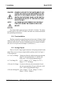
Thermal Conductivity Analyzer
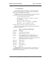
OPERATING INSTRUCTIONS FOR
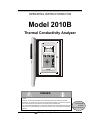
Model 2010B
Thermal Conductivity Analyzer
Teledyne A nalytical In strum ents
0.0
AL-1
%
Anlz
2010B
Therm al C onductivity A nalyzer
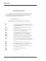
DANGER
HIGHLY TOXIC AND OR FLAMMABLE LIQUIDS OR GASES MAY BE PRESENT IN THIS MONITORING
SYSTEM.
PERSONAL PROTECTIVE EQUIPMENT MAY BE REQUIRED WHEN SERVICING THIS SYSTEM.
HAZARDOUS VOLTAGES EXIST ON CERTAIN COMPONENTS INTERNALLY WHICH MAY PERSIST
FOR A TIME EVEN AFTER THE POWER IS TURNED OFF AND DISCONNECTED.
ONLY AUTHORIZED PERSONNEL SHOULD CONDUCT MAINTENANCE AND/OR SERVICING. BEFORE
CONDUCTING ANY MAINTENANCE OR SERVICING CONSULT WITH AUTHORIZED SUPERVISOR/
MANAGER.
Teledyne Analytical Instruments
P/N M70845
11/22/00
ECO # 00-0517
i
Model 2010B
Copyright © 1998 Teledyne Analytical Instruments
All Rights Reserved. No part of this manual may be reproduced, transmitted,
transcribed, stored in a retrieval system, or translated into any other language or computer
language in whole or in part, in any form or by any means, whether it be electronic,
mechanical, magnetic, optical, manual, or otherwise, without the prior written consent of
Teledyne Analytical Instruments, 16830 Chestnut Street, City of Industry, CA 917491580.
Warranty
This equipment is sold subject to the mutual agreement that it is warranted by us free
from defects of material and of construction, and that our liability shall be limited to
replacing or repairing at our factory (without charge, except for transportation), or at
customer plant at our option, any material or construction in which defects become
apparent within one year from the date of shipment, except in cases where quotations or
acknowledgments provide for a shorter period. Components manufactured by others bear
the warranty of their manufacturer. This warranty does not cover defects caused by wear,
accident, misuse, neglect or repairs other than those performed by Teledyne or an authorized service center. We assume no liability for direct or indirect damages of any kind and
the purchaser by the acceptance of the equipment will assume all liability for any damage
which may result from its use or misuse.
We reserve the right to employ any suitable material in the manufacture of our
apparatus, and to make any alterations in the dimensions, shape or weight of any parts, in
so far as such alterations do not adversely affect our warranty.
Important Notice
This instrument provides measurement readings to its user, and serves as a tool by
which valuable data can be gathered. The information provided by the instrument may
assist the user in eliminating potential hazards caused by his process; however, it is
essential that all personnel involved in the use of the instrument or its interface, with the
process being measured, be properly trained in the process itself, as well as all instrumentation related to it.
The safety of personnel is ultimately the responsibility of those who control process
conditions. While this instrument may be able to provide early warning of imminent
danger, it has no control over process conditions, and it can be misused. In particular, any
alarm or control systems installed must be tested and understood, both as to how they
operate and as to how they can be defeated. Any safeguards required such as locks, labels,
or redundancy, must be provided by the user or specifically requested of Teledyne at the
time the order is placed.
Therefore, the purchaser must be aware of the hazardous process conditions. The
purchaser is responsible for the training of personnel, for providing hazard warning
methods and instrumentation per the appropriate standards, and for ensuring that hazard
warning devices and instrumentation are maintained and operated properly.
Teledyne Analytical Instruments, the manufacturer of this instrument, cannot
accept responsibility for conditions beyond its knowledge and control. No statement
expressed or implied by this document or any information disseminated by the manufacturer or its agents, is to be construed as a warranty of adequate safety control under the user’s
process conditions.
ii
Teledyne Analytical Instruments
Thermal Conductivity Analyzer
Table of Contents
Specific Model Information ................................. iv
Part I: Control Unit, Model 2010B ......... Part I: 1-1
Part II: Analysis Unit, Model 2010B ...... Part II: 1-1
Appendix ......................................................... A-1
Teledyne Analytical Instruments
iii
Model 2010B
Specific Model Information
The instrument for which this manual was supplied may incorporate one or more
options not supplied in the standard instrument. Commonly available options are listed
below, with check boxes. Any that are incorporated in the instrument for which this
manual is supplied are indicated by a check mark in the box.
Instrument Serial Number: _______________________
Options Included in the Instrument with the Above Serial Number:
iv
❑ C:
Auto Calibration valves (zero/span/sample) built-in gas control
valves are electronically controlled to provide synchronization
with the analyzer’s operations.
❑ G:
Stainless steel cell block with nickel filaments and Stainless
Steel fittings and tubing.
❑ H:
Stainless steel cell block with gold filaments for corrosive gas
streams and Stainless Steel fittings and tubing.
❑ K:
19" Rack Mount option with one or two analyzer Control
Units installed and ready to mount in a standard rack.
❑ K2:
19" Rack Mount option with two Control Units mounted.
❑ K3:
19" Rack Mount option with one Control Unit mounted and a
blank cover installed in the second Control Unit location.
❑ L:
Gas selector panel consisting of sample/ref flow meters and
control valves for metering input of sample/calibrations support
gases.
❑ F:
Flame Arrestors for Class 1, Div. 1, Groups C/D service.
❑ P:
Flame Arrestors for Class 1, Div. 1, Groups C/D service, and
Auto Cal valves option (Ref. C above) and GP use.
❑ Q:
Flame Arrestors for Group B (hydrogen) service, and Auto Cal
valves option (Ref. C above)
❑ O:
Flame Arrestors for Group B (hydrogen)
❑ R:
Sealed Reference Cell
Teledyne Analytical Instruments
Thermal Conductivity Analyzer
Table of Contents
1 Introduction
1.1
1.2
1.3
1.4
1.5
1.6
1.7
1.8
Overview ........................................................................
Typical Applications .......................................................
Main Features of the Analyzer .......................................
Model Designations .......................................................
Operator Interface (Front Panel) ....................................
Recognizing Difference Between LCD & VFD ...............
Equipment Interface (Rear Panel)..................................
Gas Connections ...........................................................
1-1
1-2
1-2
1-3
1-3
1-5
1-5
1-7
2 Operational Theory
2.1 Introduction ....................................................................
2.2 Sensor Theory ...............................................................
2.2.1 Sensor Configuration ..............................................
2.2.2 Calibration ...............................................................
2.2.3 Effects of Flowrate and Gas Density .......................
2.2.4 Measurement Results .............................................
2.3 Electronics and Signal Processing ................................
2.4 Temperature Control ......................................................
2-1
2-1
2-1
2-2
2-3
2-3
2-3
2-5
3 Installation
3.1 Unpacking the Analyzer ................................................. 3-1
3.2 Mounting the Control Unit .............................................. 3-1
3.3 Electrical Connections (Rear Panel) .............................. 3-3
3.3.1 Primary Input Power .............................................. 3-4
3.3.2 Fuse Installation..................................................... 3-4
3.3.3 Analog Outputs ...................................................... 3-4
3.3.4 Alarm Relays ......................................................... 3-6
3.3.5 Digital Remote Cal Inputs ...................................... 3-7
3.3.6 Range ID Relays .................................................... 3-8
3.3.7 Network I/O ............................................................ 3-8
3.3.8 RS-232 Port ........................................................... 3-9
3.3.9 Remote Probe Connector ...................................... 3-9
3.4 Testing the System ........................................................ 3-16
3.5 Warm Up at Power Up ................................................... 3-16
4 Operation
4.1 Introduction .................................................................... 4-1
4.2 Using the Data Entry and Function Buttons ................... 4-1
Teledyne Analytical Instruments
v
Model 2010B
4.3 The System Function ..................................................... 4-4
4.3.1 Setting the Display ................................................. 4-5
4.3.2 Setting up an Auto-Cal ........................................... 4-5
4.3.3 Password Protection .............................................. 4-6
4.3.3.1 Entering the Password ................................... 4-7
4.3.3.2 Installing or Changing the Password ............. 4-7
4.3.4 Logging Out ........................................................... 4-9
4.3.5 System Self-Diagnostic Test .................................. 4-9
4.3.6 The Model Screen ................................................. 4-10
4.3.7 Checking Linearity with Algorithm .......................... 4-10
4.4 The Zero and Span Functions ....................................... 4-11
4.4.1 Zero Cal ................................................................. 4-12
4.4.1.1 Auto Mode Zeroing ........................................ 4-12
4.4.1.2 Manual Mode Zeroing .................................... 4-13
4.4.1.3 Cell Failure ..................................................... 4-14
4.4.2 Span Cal ................................................................ 4-14
4.4.2.1 Auto Mode Spanning ..................................... 4-15
4.4.2.2 Manual Mode Spanning ................................. 4-15
4.5 The Alarms Function ...................................................... 4-16
4.6 The Range Select Function ........................................... 4-18
4.6.1 Manual (Select/Define Range) Screen .................. 4-19
4.6.2 Auto (Single Application) Screen ........................... 4-19
4.6.3 Precautions ............................................................ 4-21
4.7 The Analyze Function .................................................... 4-21
4.8 Programming ................................................................. 4-22
4.8.1 The Set Range Screen .......................................... 4-23
4.8.2 The Curve Algorithm Screen ................................. 4-25
4.8.2.1 Checking the Linearization ............................ 4-25
4.8.2.2 Manual Mode Linearization............................ 4-26
4.8.2.3 Auto Mode Linearization ................................ 4-27
4.9 Special Function Setup .................................................. 4-28
4.9.1 Output Signal Reversal .......................................... 4.28
4.9.2 Special - Inverting Output ...................................... 4-28
4.9.3 Special - Polarity Coding ........................................ 4-29
4.9.4 Special - Nonlinear Application Gain Preset .......... 4-29
Maintenance
5.1
5.2
5.3
5.4
vi
Routine Maintenance ..................................................... 5-1
System Self Diagnostic Test........................................... 5-1
VFD Display ................................................................... 5-2
Fuse Replacement ......................................................... 5-2
Teledyne Analytical Instruments
Thermal Conductivity Analyzer
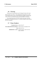
5.5 Major Internal Components ........................................... 5-3
5.6 Cleaning ......................................................................... 5-5
5.7 Phone Numbers ............................................................. 5-5
Appendix
A-1 Specifications ................................................................. A-1
A-2 Recommended 2-Year Spare Parts List ......................... A-3
A-3 Drawing List ................................................................... A-4
Teledyne Analytical Instruments
vii
Model 2010B
DANGER
COMBUSTIBLE GAS USAGE WARNING
The customer should ensure that the principles of operating of
this equipment are well understood by the user. Misuse of this
product in any manner, tampering with its components, or
unauthorized substitution of any component may adversely
affect the safety of this instrument.
Since the use of this instrument is beyond the control of
Teledyne, no responsibility by Teledyne, its affiliates, and
agents for damage or injury from misuse or neglect of this
equipment is implied or assumed.
viii
Teledyne Analytical Instruments
Thermal Conductivity Analyzer
Part I: Control Unit
Introduction
1.1
Overview
The Model 2010 is a family of split configuration conductivity analyzers.
Each analyzer consist of a Control Unit suitable for installation in a general
purpose area-enclosure rated NEMA-4, and a Analysis Unit which is housed in
an explosion-proof enclosure. The Analysis Unit enclosure is rated for NEMA
4/7 Class I, Div. 1, Groups B,C,D and is approved by U/L and CSA.
The Analytical Instruments Model 2010B Thermal Conductivity Analyzer is
a versatile microprocessor-based instrument for measuring a component gas in a
background gas, or in a specific mixture of background gases. It compares the
thermal conductivity of a sample stream with that of a reference gas of known
composition. The 2010B can—
• measure the concentration of one gas in a mixture of two gases.
• measure the concentration of a gas in a specific mixture of background gases.
• measure the purity of a sample stream containing a single impurity or a mixture of impurities.
The standard 2010B is pre-programmed with automatic linearization
algorithms for a large number of gases and gas mixtures. The factory can add to
this data base for custom applications, and the sophisticated user can add his
own unique applications.
This manual section covers the Model 2010B General Purpose flush-panel
and rack-mount control units only.
Many of the Model 2010B features covered in this manual are optional,
selected according to the customers specific application. Refer to the specific
model information sheet (page IV) for the options incorporated in the instrument.
Teledyne Analytical Instruments
Part I 1-1
Model 2010B
1 Introduction
1.2
Typical Applications
A few typical applications of the Model 2010B are:
• Power generation
• Air liquefaction
• Chemical reaction monitoring
• Steel manufacturing and heat treating
• Petrochemical process control
• Quality assurance
• Refrigeration and storage
• Gas proportioning control.
1.3
Main Features of the Analyzer
The main features of the Model 2010B Thermal Conductivity Analyzer
include:
•
Three independent, user definable, analysis ranges allow up to
three different gas applications with one concentration range
each, or up to three concentration ranges for a single gas application, or any combination.
•
Special recalibration range for multiple applications. Recalibrating one, recalibrates all.
•
Automatic, independent linearization for each range.
•
Auto Ranging allows analyzer to automatically select the proper
preset range for a given single application. Manual override
allows the user to lock onto a specific range of interest.
•
RS-232 serial digital port for use with a computer or other digital
communications device.
•
Six adjustable concentration set points with two alarms and a system
failure alarm relay.
•
Extensive self-diagnostic testing, at startup and on demand.
•
A 2-line alphanumeric display screen, driven by microprocessor
electronics, that continuously prompts and informs the operator.
•
High resolution, accurate indication of target or impurity gas
concentration from large, bright, meter readout. (0-9999 ppm
through 0-100 % depending on types of gas involved.)
•
Standard, proven sensor cell design.
1-2 Part I
Teledyne Analytical Instruments
Thermal Conductivity Analyzer
Part I: Control Unit
•
Wide range of custom applications, ranges, and linearization.
•
Microprocessor based electronics: 8-bit CMOS microprocessor
with 32 kB RAM and 128 kB ROM.
•
Auto and remote calibration capabilities.
•
Four analog outputs: two for measurement (0–1 V dc and Isolated 4–20 mA dc) and two for range identification.
•
Compact and versatile design: Small footprint, yet internal components are accessible.
1.4
Model Designations
The Model 2010B is ordinarily custom programmed at the factory to fit the
customer’s application. Many parameters, including the number of channels, the
gas application, the materials specification of the sampling system, and others,
are options. The most common options, are covered in this manual. See the
Specific Model Information checklist in the front matter of this manual for those
that apply to your Model 2010B analyzer. Some standard models that are not
covered in this manual are listed here.
Models 2000A:
Both analysis section and control unit are in a single
general purpose enclosure.
Models 2020:
Both the analysis section and control unit are in a single
explosion proof enclosure.
1.5
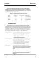
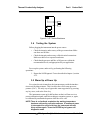
Operator Interface (Front Panel)
The standard 2010B is housed in a rugged metal case with all controls and
displays accessible from the front panel. See Figure 1-1. The front panel has
thirteen buttons for operating the analyzer, a digital meter, and an alphanumeric
display. They are described briefly here and in detail in the Operations chapter
of this manual.
Function Keys: Six touch-sensitive membrane switches are used to
change the specific function performed by the analyzer:
•
Analyze
Perform analysis for target-gas content of a sample
gas.
•
System
Perform system-related tasks (described in detail in
chapter 4, Operation.).
Teledyne Analytical Instruments
Part I 1-3
Model 2010B
1 Introduction
O u te r D o or
(O pe n)
Teledyne An alytical Instrum ents
V iew in g
W in dow
0.0
AL-1
%
Anlz
D ig ital
M ete r
LC D
S creen
In ne r D o or
Latch
(P ressing the latch button
w ill open the inn er D oor)
O u te r D o or
Latch
C ontrol
Pan el
2010B
T he rm al C o ndu ctivity A na lyzer
Figure 1-1: Model 2010B Front Panel
•
Span
Span calibrate the analyzer.
•
Zero
Zero calibrate the analyzer.
•
Alarms
Set the alarm setpoints and attributes.
•
Range
Set up the user definable ranges for the instrument.
Data Entry Keys: Six touch-sensitive membrane switches are used to
input data to the instrument via the alphanumeric VFD (Vacuum Fluorescent
Display) display:
•
Left & Right Arrows
Select between functions currently
displayed on the VFD screen.
•
Up & Down Arrows
Increment or decrement values of
functions currently displayed.
•
Enter
•
Escape Moves VFD back to the previous screen in a series. If
none remains, returns to the Analyze screen.
1-4 Part I
Moves VFD on to the next screen in a series. If none
remains, returns to the Analyze screen.
Teledyne Analytical Instruments
Thermal Conductivity Analyzer
Part I: Control Unit
Digital Meter Display: The meter display is a VFD device that
produces large, bright, 7-segment numbers that are legible in any lighting. It
produces a continuous trace readout from 0-9999 ppm or a continuous percent
readout from 1-100 %. It is accurate across all analysis ranges.
Alphanumeric Interface Screen: The VDF screen is an easy-to-use
interface between operator and analyzer. It displays values, options, and
messages that give the operator immediate feedback.
Standby Button: The Standby turns off the display and outputs,
but circuitry is still operating.
CAUTION: The power cable must be unplugged to fully
disconnect power from the instrument. When
chassis is exposed or when access door is open
and power cable is connected, use extra care to
avoid contact with live electrical circuits.
Access Door: For access to the thermal conductivity sensor or the front
panel electronics, the front panel swings open when the latch in the upper right
corner of the panel is pressed all the way in with a narrow gauge tool. Accessing
the main electronics circuit board requires unfastening rear panel screws and
sliding the electronics drawer out of the case. (See chapter 5.)
1.6
Recognizing Difference Between LCD &
VFD
LCD (Liquid Crystal Display) has GREEN background with BLACK
characters. VFD has DARK background with GREEN characters. In the case
of VFD (Vacuum Fluorescent Display) - NO CONTRAST ADJUSTMENT IS
NEEDED.
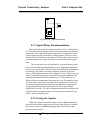
1.7
Equipment Interface (Rear Panel)
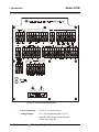
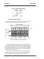
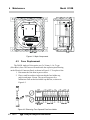
The rear panel, shown in Figure 1-2, contains the electrical connectors for
external input and output. The connectors are described briefly here and in detail
in chapter 3, Installation.
Teledyne Analytical Instruments
Part I 1-5
Model 2010B
1 Introduction
Figure 1-2: Model 2010B Rear Panel
•
Power Connection
85-250 V AC power source.
•
Analog Outputs
0-1 V dc concentration plus 0-1 V dc
range ID, and isolated 4-20 mA dc plus
4-20 mA dc range ID.
1-6 Part I
Teledyne Analytical Instruments
Thermal Conductivity Analyzer
Part I: Control Unit
•
Alarm Connections
2 concentration alarms and 1 system
alarm.
•
RS-232 Port
Serial digital concentration signal output
and control input.
•
Remote Probe
Used in the 2010B to interface the
external Analysis Unit.
•
Remote Span/Zero
Digital inputs allow external control of
analyzer calibration.
•
Calibration Contact
To notify external equipment that
instrument is being calibrated and
readings are not monitoring sample.
•
Range ID Contacts
Four separate, dedicated,
range-identification relay contacts (01,
02, 03,CAL).
•
Network I/O
Serial digital communications for local
network access. For future expansion.
Not implemented at this printing.
Note: If you require highly accurate Auto-Cal timing, use external
Auto-Cal control where possible. The internal clock in the
Model 2010B is accurate to 2-3 %. Accordingly, internally
scheduled calibrations can vary 2-3 % per day.
Teledyne Analytical Instruments
Part I 1-7
Model 2010B
1 Introduction
1-8 Part I
Teledyne Analytical Instruments
Thermal Conductivity Analyzer
Part I: Control Unit
Operational Theory
2.1
Introduction
The analyzer is composed of two subsystems:
1. Thermal Conductivity Sensor
2. Electronic Signal Processing, Display and Control.
The sensor is a thermal conductivity comparator that continuously
compares the thermal conductivity of the sample gas with that of a reference
gas having a known conductivity.
The electronic signal processing, display and control subsystem simplifies operation of the analyzer and accurately processes the sampled data. A
microprocessor controls all signal processing, input/output, and display
functions for the analyzer.
2.2
Sensor Theory
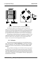
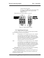
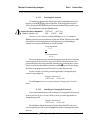
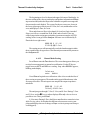
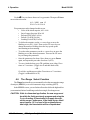
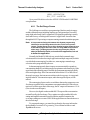
For greater clarity, Figure 2-1 presents two different illustrations, (a)
and (b), of the operating principle of the thermal conductivity cell.
2.2.1 Sensor Configuration
The thermal conductivity sensor contains two chambers, one for the
reference gas of known conductivity and one for the sample gas. Each
chamber contains a pair of heated filaments. Depending on its thermal
conductivity, each of the gases conducts a quantity of heat away from the
filaments in its chamber. See Figure 2-1(a).
The resistance of the filaments depends on their temperature. These
filaments are parts of the two legs of a Wheatstone bridge circuit that unbalances if the resistances of its two legs do not match. See Figure 2-1(b).
Teledyne Analytical Instruments
Part I 2-1
2 Operational Theory
Model 2010B
Figure 2-1: Thermal Conductivity Cell Operating Principle
If the thermal conductivities of the gases in the two chambers are
different, the Wheatstone bridge circuit unbalances, causing a current to flow
in its detector circuit. The amount of this current can be an indication of the
amount of impurity in the sample gas, or even an indication of the type of
gas, depending on the known properties of the reference and sample gases.
The temperature of the measuring cell is regulated to within 0.1 °C by a
sophisticated control circuit. Temperature control is precise enough to compensate for diurnal effects in the output over the operating ranges of the
analyzer. (See Specifications in the Appendix for details.)
2.2.2 Calibration
Because analysis by thermal conductivity is not an absolute measurement, calibration gases of known composition are required to fix the upper
and lower parameters (“zero” and “span”) of the range, or ranges, of analysis. These gases must be used periodically, to check the accuracy of the
analyzer.
During calibration, the bridge circuit is balanced, with zero gas against
the reference gas, at one end of the measurement range; and it is sensitized
with span gas against the reference gas at the other end of the measurement
range. The resulting electrical signals are processed by the analyzer electronics to produce a standard 0-1V, or an isolated 4–20 mA dc, output signal, as
described in the next section.
2-2 Part I
Teledyne Analytical Instruments
Thermal Conductivity Analyzer
Part I: Control Unit
2.2.3 Effects of Flowrate and Gas Density
Because the flowrate of the gases in the chambers affects their cooling
of the heated filaments, the flowrate in the chambers must be kept as equal,
constant, and low as possible.
When setting the sample and reference flowrate, note that gases lighter
than air will have an actual flowrate higher than indicated on the flowmeter,
while gases heavier than air will have an actual flowrate lower than indicated. Due to the wide range of gases that are measured with the Thermal
Conductivity Analyzer, the densities of the gases being handled may vary
considerably.
Then, there are limited applications where the reference gas is in a
sealed chamber and does not flow at all. These effects must be taken in
consideration by the user when setting up an analysis.
2.2.4 Measurement Results
Thermal conductivity measurements are nonspecific by nature. This fact
imposes certain limitations and requirements. If the user intends to employ
the analyzer to detect a specific component in a sample stream, the sample
must be composed of the component of interest and one other gas (or specific, and constant, mixture of gases) in order for the measured heat-transfer
differences to be nonambiguous.
If, on the other hand, the user is primarily interested in the purity of a
process stream, and does not require specific identification of the impurity,
the analyzer can be used on more complex mixtures.
2.3
Electronics and Signal Processing
The Model 2010B Thermal Conductivity Analyzer uses an 8031
microcontroller, Central Processing Unit—(CPU) with 32 kB of RAM and
128 kB of ROM to control all signal processing, input/output, and display
functions for the analyzer. System power is supplied from a universal power
supply module designed to be compatible with any international power
source. (See Major Internal Components in chapter 5 Maintenance for the
location of the power supply and the main electronic PC boards.)
The signal processing electronics including the microprocessor, analog
to digital, and digital to analog converters are located on the Motherboard at
the bottom of the case. The Preamplifier board is mounted on top of the
Motherboard as shown in the figure 5.4. These boards are accessible after
Teledyne Analytical Instruments
Part I 2-3
2 Operational Theory
Model 2010B
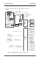
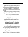
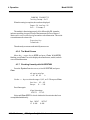
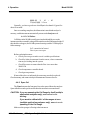
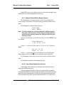
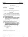
removing the back panel. Figure 2-2 is a block diagram of the Analyzer
electronics.
Differential
Amplifier
Variable
Gain
Amplifier
Thermistor
A to D
Converter
To CPU
M
U
X
Sensor
Heater
AutoRange
Temperature
Control
Temperature
Control
Heater
Fine
Adjustment
Coarse
Adjustment
Digitial to
Analog
Converter
(DAC)
0-1 V dc
Concentration
and Range
4-20 mA dc
Concentration
and Range
Alarm 1
Alarm 2
Selt-Test Signal to MUX
System
Failure
Alarm
RS-232
Keyboard
Central
Processing
Unit
(CPU)
Displays
Processing
Range
Contacts (4)
External
Valve
Control
Remote Span
Control
Power
Supply
A to D Conv
Remote Zero
Control
Cal
Contact
Figure 2-2: Block Diagram of the Model 2010B Electronics
2-4 Part I
Teledyne Analytical Instruments
Thermal Conductivity Analyzer
Part I: Control Unit
In the presence of dissimilar gases the sensor generates a differential
voltage across its output terminals. A differential amplifier converts this
signal to a unipolar signal, which is amplified in the second stage, variable
gain amplifier, which provides automatic range switching under control of
the CPU. The output from the variable gain amplifier is sent to an 18 bit
analog to digital converter.
The digital concentration signal along with input from the Gas Selector
Panel is processed by the CPU and passed on to the 12-bit DAC, which
outputs 0-1 V dc Concentration and Range ID signals. An voltage-to-current
converter provides 4-20 mA dc concentration signal and range ID outputs.
The CPU also provides appropriate control signals to the Displays,
Alarms, and External Valve Controls, and accepts digital inputs for external
Remote Zero and Remote Span commands. It monitors the power supply
through an analog to digital converter as part of the data for the system
failure alarm.
The RS-232 port provides two-way serial digital communications to
and from the CPU. These, and all of the above electrical interface signals are
described in detail in chapter 3 Installation.
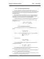
2.4. Temperature Control
For accurate analysis the sensor of this instrument is temperature controlled to 50oC.
The Temperature Control keeps the temperature of the measuring cell
regulated to within 0.1 degree C. A thermistor is used to measure the temperature, and a zero-crossing switch regulates the power in a cartridge-type
heater. The result is a sensor output signal that is temperature independent.
A second temperature control system is used to maintain the Analysis
Unit internal temperature at 220C minimum.
Teledyne Analytical Instruments
Part I 2-5
2 Operational Theory
2-6 Part I
Teledyne Analytical Instruments
Model 2010B
Thermal Conductivity Analyzer
Part I: Control Unit
Installation
Installation of the Model 2010B Analyzer includes:
1. Unpacking
2. Mounting
3. Gas connections
4. Electrical connections
5. Testing the system.
3.1
Unpacking the Analyzer
The analyzer is shipped ready to install and prepared for operation.
Carefully unpack the analyzer and inspect it for damage. Immediately report
any damage to the shipping agent.
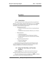
3.2
Mounting the Control Unit
The Model 2010B Control Unit is designed for bulkhead mounting in
general purpose area, NOT for hazardous environments of any type. The
Control Unit is for indoor/outdoor use.
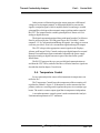
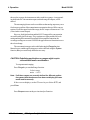
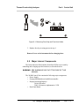
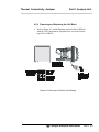
Figure 3-1 is an illustration of the 2010B standard front panel and
mounting bezel. There are four mounting holes—one in each corner of the
rigid frame. See the outline drawing, at the back of this manual for overall
dimensions.
All operator controls are mounted on the inner control panel, which is
hinged on the left edge and doubles as a door to provide access to the internal
components of the instrument. The door will swing open when the button of
the latch is pressed all the way in with a narrow gauge tool (less than 0.18
inch wide), such as a small hex wrench or screwdriver Allow clearance for
the door to open in a 90-degree arc of radius 11.75 inches. See Figure 3-2.
Teledyne Analytical Instruments
Part I 3-1
3 Installation
Model 2010B
N P T Fittings
supplied by
custo m e r
V iew ing
W indow
0.0
AL-1
% Anlz
O u ter D oor
Latch
HHinge
Figure 3-1: Front Panel of the Model 2010B Control Unit
.75
11
in
Figure 3-2: Required Front Door Clearance
H
3-2 Part I
Teledyne Analytical Instruments
Thermal Conductivity Analyzer
3.3
Part I: Control Unit
Electrical Connections (Rear Panel)
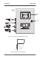
Figure 3-3 shows the Model 2010B Electrical Connector Panel. There
are terminal blocks for connecting power, communications, and both digital
and analog concentration outputs.
For safe connections, ensure that no uninsulated wire extends outside of
the connectors they are attached to. Stripped wire ends must insert completely into terminal blocks. No uninsulated wiring should be able to come in
contact with fingers, tools or clothing during normal operation.
Figure 3-3: Rear Panel of the Model 2010B
3.3.1 Primary Input Power
The power terminal block and fuse receptacles are located in the same
rear panel assembly.
Teledyne Analytical Instruments
Part I 3-3
3 Installation
Model 2010B
DANGER: POWER IS APPLIED TO THE INSTRUMENT'S CIRCUITRY AS LONG AS THE INSTRUMENT IS CONNECTED TO THE POWER SOURCE. THE RED I/O
SWITCH ON THE FRONT PANEL IS FOR SWITCHING POWER ON OR OFF TO THE DISPLAYS AND
OUTPUTS ONLY.
NOTE:
AC POWER MAY BE PRESENT ON THE RELAY
CONTACTS WHEN THE POWER CORD IS REMOVED!
The Control Unit is universal power 100-240V, 50-60 Hz. The Analysis Unit requires 110 or 220 VAC and is selectable via switch located inside
the explosion-proof enclosure.
3.3.2 Fuse Installation
The fuse receptacles accepts European size fuses only (5x20mm). Both
sides of the line are fused. If the European size fuses are selected, both sides
at the line will be fused. Be sure to install the proper fuse as part of installation. (See Fuse Replacement in chapter 5, maintenance.)
3.3.3 Analog Outputs
There are four DC output signal connectors with spring terminals on the
panel. There are two wires per output with the polarity noted. See Figure 34. The outputs are:
0–1 V dc % of Range: Voltage rises linearly with increasing concentration,
from 0 V at 0 concentration to 1 V at full scale.
(Full scale = 100% of programmable range.)
0–1 V dc Range ID:
0.25 V = Range 1, 0.5 V = Range 2, 0.75 V =
Range 3, 1 V = Cal Range.
4–20 mA dc % Range: Current rises linearly with concentration, from 4
mA at 0 concentration to 20 mA at full scale. (Full
scale = 100% of programmable range.)
4–20 mA dc Range ID: 8 mA = Range 1, 12 mA = Range 2, 16 mA =
Range 3, 20 mA = Range 4.
3-4 Part I
Teledyne Analytical Instruments
Thermal Conductivity Analyzer
Part I: Control Unit
Figure 3-4: Analog Output Connections
Examples:
The analog output signal has a voltage which depends on gas concentration relative to the full scale of the range. To relate the signal output to the
actual concentration, it is necessary to know what range the instrument is
currently on, especially when the analyzer is in the autoranging mode.
The signal output for concentration is linear over the currently selected
analysis range. For example, if the analyzer is set on a range that was defined
as 0–10 % hydrogen, then the output would be as shown in Table 3-1.
Table 3-1: Analog Concentration Output—Example
Percent
Hydrogen
Voltage Signal
Output (V dc)
0
1
2
3
4
5
6
7
8
9
10
0.0
0.1
0.2
0.3
0.4
0.5
0.6
0.7
0.8
0.9
1.0
Current Signal
Output (mA dc)
4.0
5.6
7.2
8.8
10.4
12.0
13.6
15.2
16.8
18.4
20.0
(Continued)
Teledyne Analytical Instruments
Part I 3-5
3 Installation
Model 2010B
To provide an indication of the range, the Range ID analog output
terminals are used. They generate a steady preset voltage (or current when
using the current outputs) to represent a particular range. Table 3-2 gives the
range ID output for each analysis range.
Table 3-2: Analog Range ID Output—Example
Range
Range 1
Voltage (V)
0.25
Current (mA) Application
8
0-1 % H2 in N2
Range 2
0.50
12
0-10 % H2 in N2
Range 3
0.75
16
0-1 % H2 in Air
Range 4 (Cal)
1.00
20
0-1 % H2 in N2
3.3.4 Alarm Relays
The three alarm-circuit connectors are spring terminals for making
connections to internal alarm relay contacts. Each provides a set of Form C
contacts for each type of alarm. Each has both normally open and normally
closed contact connections. The contact connections are indicated by diagrams on the rear panel. They are capable of switching up to 3 amperes at
250 V ac into a resistive load. See Figure 3-5. The connectors are:
Threshold Alarm 1:
• Can be configured as high (actuates when concentration is above threshold), or low (actuates when
concentration is below threshold).
• Can be configured as fail-safe or non-fail-safe.
• Can be configured as latching or nonlatching.
• Can be configured out (defeated).
Threshold Alarm 2:
• Can be configured as high (actuates when concentration is above threshold), or low (actuates when
concentration is below threshold).
• Can be configured as fail-safe or non-fail-safe.
• Can be configured as latching or nonlatching.
• Can be configured out (defeated).
System Alarm:
Actuates when DC power supplied to circuits is
unacceptable in one or more parameters. Permanently
configured as fail-safe and latching. Cannot be defeated.
Actuates when cell can not balance during zero
calibration.
Actuates when span parameter out off its limited
parameter.
3-6 Part I
Teledyne Analytical Instruments
Thermal Conductivity Analyzer
Part I: Control Unit
Actuates when self test fails.
(Reset by pressing I/O button to remove power. Then
press I/O again and any other button EXCEPT
System to resume.
Further detail can be found in chapter 4, section 4-5.
Figure 3-5: Types of Relay Contacts
3.3.5 Digital Remote Cal Inputs
Accept 0 V (off) or 24 V dc (on) inputs for remote control of calibration. (See Remote Calibration Protocol below.)
Zero:
Floating input. 5 to 24 V input across the + and – terminals
puts the analyzer into the Zero mode. Either side may be
grounded at the source of the signal. A synchronous signal
must open and close the external gas control valves appropriately. See 3.3.9 Remote Probe Connector. (With the –C
option, the internal valves operate automatically.)
Span:
Floating input. 5 to 24 V input across the + and – terminals
puts the analyzer into the Span mode. Either side may be
grounded at the source of the signal. A synchronous signal
must open and close the external gas control valves appropriately. See 3.3.9 Remote Probe Connector. (With the –C
option, the internal valves operate automatically.)
Cal Contact: This relay contact is closed while analyzer is spanning
and/or zeroing. (See Remote Calibration Protocol below.)
Remote Calibration Protocol: To properly time the Digital Remote
Cal Inputs to the Model 2010B Analyzer, the customer's controller must
monitor the Cal Relay Contact.
Teledyne Analytical Instruments
Part I 3-7
3 Installation
Model 2010B
When the contact is OPEN, the analyzer is analyzing, the Remote Cal
Inputs are being polled, and a zero or span command can be sent.
When the contact is CLOSED, the analyzer is already calibrating. It
will ignore your request to calibrate, and it will not remember that request.
Once a zero or span command is sent, and acknowledged (contact
closes), release it. If the command is continued until after the zero or span is
complete, the calibration will repeat and the Cal Relay Contact (CRC) will
close again.
When the contact is closed, the display would display the last reading of
the gas concentration value and output signal would output the last reading
from the sample gas (SAMPLE and HOLD).
For example:
1) Test the CRC. When the CRC is open, Send a zero command
until the CRC closes (The CRC will close quickly.)
2) When the CRC closes, remove the zero command.
3) When CRC opens again, send a span command until the CRC
closes. (The CRC will close quickly.)
4) When the CRC closes, remove the span command.
When CRC opens again, zero and span are done, and the sample is
being analyzed.
Note: The Remote Probe connector (paragraph 3.3.9) provides
signals to operate the zero and span gas valves synchronously. However, if you have the –C, -P, or -Q Internal valve
option, which includes zero and span gas inputs, the 2010B
automatically selects the zero, span and sample gas flow.
3.3.6 Range ID Relays
Four dedicated Range ID relay contacts. For any single application they
are assigned to relays in ascending order. For example: if all ranges have the
same application, then the lowest range is assigned to the Range 1 ID relay,
and the highest range is assigned to the Range 3 ID relay. Range 4 is the Cal
Range ID relay.
3.3.7 Network I/O
A serial digital input/output for local network protocol. At this printing,
this port is not yet functional. It is to be used in future versions of the instrument.
3-8 Part I
Teledyne Analytical Instruments
Thermal Conductivity Analyzer
Part I: Control Unit
3.3.8 RS-232 Port
The digital signal output is a standard RS-232 serial communications
port used to connect the analyzer to a computer, terminal, or other digital
device. It requires a standard 9-pin D connector.
Output: The data output is status information, in digital form, updated
every two seconds. Status is reported in the following order:
• The concentration in ppm or percent
• The range in use (01 = Range 1, 02 = Range 2, 03 = Range 3,
CAL = Range 4)
• The scale of the range (0-100 %, etc)
•
•
Which alarms—if any—are disabled (AL–x DISABLED)
Which alarms—if any—are tripped (AL–x ON).
Each status output is followed by a carriage return and line feed.
Input: The input functions using RS-232 that have been implemented
to date are described in Table 3-3.
Table 3-3: Commands via RS-232 Input
Command
Description
as<enter>
Immediately starts an autospan.
az<enter>
Immediately starts an autozero.
rp<enter>
Allows reprogramming of the APPLICATION (gas use)
and ALGORITHM (linearization) System functions.
st<enter>
Toggling input. Stops/Starts any status message output from
the RS-232, until st<enter> is sent again.
rm1<enter>
Range manual 1
rm2<enter>
Range manual 2
rm3<enter>
Range manual 3
rm4<enter>
Range manual CAL
ra<enter>
Range auto
Implementation: The RS-232 protocol allows some flexibility in its
implementation. Table 3-4 lists certain RS-232 values that are required by
the Model 2010B implementation.
Teledyne Analytical Instruments
Part I 3-9
3 Installation
Model 2010B
Table 3-4: Required RS-232 Options
Parameter
Baud
Byte
Parity
Stop Bits
Message Interval
Setting
2400
8 bits
none
1
2 seconds
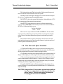
3.3.9 Remote Probe Connector
The 2010B is a single-split configuration analyzer, the Remote Probe
connector is used to interface the Analysis Unit. See Figure 3-6.
S PA N IN
S A M P L E IN
ZE RO IN
E X H AU S T
+15V
Tu rn cw to ho ld
ccw to
lo ose n w ire.
S w itch in g
G rou n d
In se rt w ire
h ere.
Figure 3-6: Remote Probe Connector Pinouts
The voltage from these outputs is nominally 0 V for the OFF and
15 V dc for the ON conditions. The maximum combined current that can be
pulled from these output lines is 100 mA. (If two lines are ON at the same
time, each must be limited to 50 mA, etc.) If more current and/or a different
voltage is required, use a relay, power amplifier, or other matching circuitry
to provide the actual driving current.
In addition, each individual line has a series FET with a nominal ON
resistance of 5 ohms (9 ohms worst case). This could limit the obtainable
voltage, depending on the load impedance applied. See Figure 3-7.
3-10 Part I
Teledyne Analytical Instruments
Thermal Conductivity Analyzer
Part I: Control Unit
Figure 3-7: FET Series Resistance
3.4
Testing the System
Before plugging the instrument into the power source:
• Check the integrity and accuracy of the gas connections. Make
sure there are no leaks.
• Check the integrity and accuracy of the electrical connections.
Make sure there are no exposed conductors
• Check that the pressure and flow of all gases are within the
recommended levels, and appropriate for your application.
Power up the system, and test it by performing the following
operations:
1. Repeat the Self-Diagnostic Test as described in chapter 4, section
4.3.5.
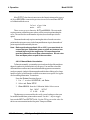
3.5 Warm Up at Power Up
Every time the unit is turned on, the instrument stays with the introduction screen for thirty minutes. This is to allow the cell to come up to temperature (50oC). The only way to bypass this warm up period is by pressing
any key once, such as the Enter key.
The instrument warms up for half an hour so that it will not receive a
remote calibration signal, send false readings to a monitor system, or, again,
be calibrated by an untrained operator while the cell is cold.
NOTE:There is no feedback on whether the working temperature
has been achieved by cell to the software. If instrument power
is interrupted for only a brief time, the instrument will wait
thirty minutes again. Press the ENTER key to bypass selfdiagnostic mode.
Teledyne Analytical Instruments
Part I 3-11
3 Installation
3-12 Part I
Model 2010B
Teledyne Analytical Instruments
Thermal Conductivity Analyzer
Part I: Control Unit
Operation
4.1
Introduction
Although the Model 2010B is usually programmed to your application at
the factory, it can be further configured at the operator level, or even, cautiously, reprogrammed. Depending on the specifics of the application, this might
include all or a subset of the following procedures:
• Setting system parameters:
• Establish a security password, if desired, requiring Operator
to log in.
• Establish and start an automatic calibration cycle, if desired.
•
•
Routine Operation:
• Calibrate the instrument.
• Choose autoranging or select a fixed range of analysis.
• Set alarm setpoints, and modes of alarm operation (latching,
fail-safe, etc).
Program/Reprogram the analyzer:
• Define new applications.
• Linearize your ranges.
If you choose not to use password protection, the default password is
automatically displayed on the password screen when you start up, and you
simply press Enter for access to all functions of the analyzer.
4.2
Using the Data Entry and Function
Buttons
Data Entry Buttons: The < > buttons select options from the menu
currently being displayed on the VFD screen. The selected option blinks.
When the selected option includes a modifiable item, the ∆ ∇ arrow buttons
can be used to increment or decrement that modifiable item.
Teledyne Analytical Instruments
Part I 4-1
4 Operation
Model 2010B
The Enter button is used to accept any new entries on the VFD screen.
The Escape button is used to abort any new entries on the VFD screen that are
not yet accepted by use of the Enter button.
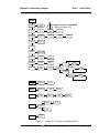
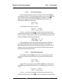
Figure 4-1 shows the hierarchy of functions available to the operator via the
function buttons. The six function buttons on the analyzer are:
• Analyze. This is the normal operating mode. The analyzer
monitors the thermal conductivity of the sample, displays the
percent or parts-per-million of target gas or contamination, and
warns of any alarm conditions.
• System. The system function consists of nine subfunctions.
Four of these are for ordinary setup and operation:
• Setup an Auto-Cal
• Assign Passwords
• Log out to secure system
• Initiate a Self-Test
Three of the subfunctions do auxiliary tasks:
• Checking model and software version
• Display more subfunctions
Two of these are for programming/reprogramming the analyzer:
• Define gas applications and ranges (Refer to programming
section, or contact factory.)
• Use the Curve Algorithm to linearize output. (Refer to
programming section, or contact factory.)
• Zero. Used to set up a zero calibration.
• Span. Used to set up a span calibration.
• Alarms. Used to set the alarm setpoints and determine whether
each alarm will be active or defeated, HI or LO acting, latching,
and/or fail-safe.
• Range. Used to set up three analysis ranges that can be
switched automatically with autoranging or used as individual
fixed ranges.
Any function can be selected at any time by pressing the appropriate button
(unless password restrictions apply). The order as presented in this manual is
appropriate for an initial setup.
Each of these functions is described in greater detail in the following procedures. The VFD screen text that accompanies each operation is reproduced, at
the appropriate point in the procedure, in a Monospaced type style. Pushbutton names are printed in Oblique type.
4-2 Part I
Teledyne Analytical Instruments
Thermal Conductivity Analyzer
Part I: Control Unit
System
CONTRAST
Set LCD
Contrast
AUTO-CAL
Span/Zero
Off/On
Span/Zero
Timing
PASSWORD
Enter
Password
Change
Yes/No
LOGOUT
Secure Sys &
Analyze Only
Contrast Function is DISABLED
(Refer to Section 1.6)
Span/Zero
Off/On
Yes
Change
Password
Verify
Password
MORE
MODEL
Show Model
and Version
APPLICATION
Select
Range
Define
Appl/Range
SELF-TEST
Self-Test in
Progress
Slef-Test
Results
ALGORITHM
Select
Range
Gas Use
Range
Ver
Select
Verify/Setup
Verify
Points
Enter
Man Input/Output
Values
Enter
Auto/Manual
Set Linearity Cal
Select Linrty
Auto Span Values
Zero
Auto/Manual
Zero Select
Zero in
Progress
Span
Auto/Manual
Span Select
Span Value
Set
Span in
Progress
Alarms
Select
Range
Gas Use
Range
% / ppm
Select
Man
Range
Setpoints &
Attributes
Define
Range
Auto/Manual
Range Adj
Auto
Analyze
Select
Range
Enter
Gas
Application
Analyze
Sample
Figure 4-1: Hierarchy of Functions and Subfunctions
Teledyne Analytical Instruments
Part I 4-3
4 Operation
Model 2010B
4.3
The System Function
The subfunctions of the System function are described below. Specific
procedures for their use follow the descriptions:
•
•
•
•
•
•
•
•
4-4 Part I
AUTO-CAL: Used to define an automatic calibration sequence
and/or start an AUTO-CAL.
PWD: Security can be established by choosing a 3 digit
password (PWD) from the standard ASCII character set. Once a
unique password is assigned and activated, the operator MUST
enter the UNIQUE password to gain access to setup functions
which alter the instrument's operation.
LOGOUT: Logging out prevents an unauthorized tampering
with analyzer settings.
MORE: Select and enter MORE to get a new screen with
additional subfunctions listed.
MODEL: Displays Manufacturer, Model, and Software Version
of instrument.
APPLICATION: A restricted function, not generally accessed by
the end user. Used to define up to three analysis ranges and a
calibration range (including impurity, background, low end of range,
high end of range, and % or ppm units).
SELF-TEST: The instrument performs a self-diagnostic test to
check the integrity of the power supply, output boards, sensor
cell, and preamplifiers.
ALGORITHM: A restricted function, not generally accessed by the
end user. Used to linearize the output for the range of interest.
Teledyne Analytical Instruments
Thermal Conductivity Analyzer
Part I: Control Unit
4.3.1 Setting the Display
Contrast Function is DISABLED
(Refer to Section 1.6)
If you cannot read anything on the VFD after first powering up:
1. Observe LED readout.
a. If LED meter reads 8.8.8.8.8., go to step 3.
b. If LED meter displays anything else, go to step 2.
2. Press I/O button twice to turn Analyzer OFF and ON again. LED
meter should now read 8.8.8.8.8.. Go to step 3.
4.3.2 Setting up an AUTO-CAL
When proper automatic valving is connected (see chapter 3, installation),
the Analyzer can cycle itself through a sequence of steps that automatically zero
and span the instrument.
Note: Before setting up an AUTO-CAL, be sure you understand the
Zero and Span functions as described in section 4.4, and
follow the precautions given there.
Note: If you require highly accurate AUTO-CAL timing, use external
AUTO-CAL control where possible. The internal clock in the
Model 2010B is accurate to 2-3 %. Accordingly, internally
scheduled calibrations can vary 2-3 % per day.
Note: If all your ranges are for the same gas application, then AUTOCAL will calibrate whichever range you are in at the scheduled
time for automatic calibration.
Note: If your ranges are configured for different applications, then
AUTO-CAL will calibrate all of the ranges simultaneously (by
calibrating the Cal Range).
To setup an Auto–Cal cycle:
Choose System from the Function buttons. TheVFD will display five
subfunctions.
Contrast Function is DISABLED CONTRAST
(Refer to Section 1.6)
PWD
LOGOUT
AUTO—CAL
MORE
Teledyne Analytical Instruments
Part I 4-5
4 Operation
Model 2010B
Use < > arrows to blink AUTO—CAL, and press Enter. A new screen for
ZERO/SPAN set appears.
ZERO in
Ød Øh off
SPAN in Ød Øh off
Press < > arrows to blink ZERO (or SPAN), then press Enter again.
(You won’t be able to set OFF to ON if a zero interval is entered.) A Span
Every ... (or Zero Every ...) screen appears.
Zero schedule: OFF
Day: Ød Hour: Øh
Use ∆ ∇ arrows to set an interval value, then use < > arrows to move to the
start-time value. Use ∆ ∇ arrows to set a start-time value.
To turn ON the SPAN and/or ZERO cycles (to activate AUTO–CAL):
Press System again, choose AUTO–CAL, and press Enter again. When the
ZERO/SPAN values screen appears, use the < > arrows to blink the ZERO
(or SPAN) and press Enter to go to the next screen. Use < > to select OFF/
ON field. Use ∆ ∇ arrows to set the OFF/ON field to ON. You can now turn
these fields ON because there is a nonzero span interval defined.
4.3.3 Password Protection
Before a unique password is assigned, the system assigns TAI by default.
This password will be displayed automatically. The operator just presses the
Enter key to be allowed total access to the instrument’s features.
If a password is assigned, then setting the following system parameters can
be done only after the password is entered: alarm setpoints, assigning a new
password, range/application selections, and curve algorithm linearization.
(APPLICATION and ALGORITHM are covered in the programming section.)
However, the instrument can still be used for analysis or for initiating a self-test
without entering the password. To defeat security the password must be
changed back to TAI.
NOTE: If you use password security, it is advisable to keep a copy of
the password in a separate, safe location.
4-6 Part I
Teledyne Analytical Instruments
Thermal Conductivity Analyzer
4.3.3.1
Part I: Control Unit
Entering the Password
To install a new password or change a previously installed password, you
must key in and ENTER the old password first. If the default password is in
effect, pressing the ENTER button will enter the default TAI password for you.
Press System to enter the System mode.
Contrast Function is DISABLED
(Refer to Section 1.6)
CONTRAST AUTO—CAL
PWD
LOGOUT
MORE
Use the < > arrow keys to scroll the blinking over to PWD, and press
Enter to select the password function. Either the default TAI password or AAA
place holders for an existing password will appear on screen depending on
whether or not a password has been previously installed.
Enter password:
TAI
or
Enter password:
AAA
The screen prompts you to enter the current password. If you are not using
password protection, press Enter to accept TAI as the default password. If a
password has been previously installed, enter the password using the < > arrow
keys to scroll back and forth between letters, and the ∆ ∇ arrow keys to change
the letters to the proper password. Press Enter to enter the password.
In a few seconds, you will be given the opportunity to change this password or keep it and go on.
Change Password?
<ENT>=Yes
<ESC>=No
Press Escape to move on, or proceed as in Changing the Password,
below.
4.3.3.2
Installing or Changing the Password
If you want to install a password, or change an existing password, proceed
as above in Entering the Password. When you are given the opportunity to
change the password:
Change Password?
<ENT>=Yes
<ESC>=No
Press Enter to change the password (either the default TAI or the previously assigned password), or press Escape to keep the existing password and
move on.
Teledyne Analytical Instruments
Part I 4-7
4 Operation
Model 2010B
If you chose Enter to change the password, the password assignment
screen appears.
Select new password
TAI
Enter the password using the < > arrow keys to move back and forth
between the existing password letters, and the ∆ ∇ arrow keys to change the
letters to the new password. The full set of 94 characters available for password
use are shown in the table below.
Characters Available for Password Definition:
A
K
U
_
i
s
}
)
3
=
B
L
V
`
j
t
→
*
4
>
C
M
W
a
k
u
!
+
5
?
D
N
X
b
l
v
"
'
6
@
E
O
Y
c
m
w
#
7
F
P
Z
d
n
x
$
.
8
G
Q
[
e
o
y
%
/
9
H
R
¥
f
p
z
&
0
:
I
S
]
g
q
{
'
1
;
J
T
^
h
r
|
(
2
<
When you have finished typing the new password, press Enter. A verification screen appears. The screen will prompt you to retype your password for
verification.
Enter PWD To Verify:
AAA
Use the arrow keys to retype your password and press Enter when
finished. Your password will be stored in the microprocessor and the system will
immediately switch to the Analyze screen, and you now have access to all
instrument functions.
If all alarms are defeated, the Analyze screen appears as:
1.95 % H2 in N2
nR1: Ø — 1Ø Anlz
If an alarm is tripped, the second line will change to show which alarm it is:
1.95
AL—1
4-8 Part I
% H2 in N2
Teledyne Analytical Instruments
Thermal Conductivity Analyzer
Part I: Control Unit
NOTE:If you log off the system using the LOGOUT function in the
system menu, you will now be required to re-enter the password to gain access to Alarm, and Range functions.
4.3.4 Logging Out
The LOGOUT function provides a convenient means of leaving the analyzer
in a password protected mode without having to shut the instrument off. By
entering LOGOUT, you effectively log off the instrument leaving the system
protected against use until the password is reentered. To log out, press the
System button to enter the System function.
Contrast Function is DISABLED
(Refer to Section 1.6)
CONTRAST
AUTO—CAL
PWD
LOGOUT
MORE
Use the < > arrow keys to position the blinking over the LOGOUT function, and press Enter to Log out. The screen will display the message:
Protected until
password entered
4.3.5 System Self-Diagnostic Test
The Model 2010B has a built-in self-diagnostic testing routine. Pre-programmed signals are sent through the power supply, output board, preamp
board and sensor circuit. The return signal is analyzed, and at the end of the test
the status of each function is displayed on the screen, either as OK or as a
number between 1 and 1024. (See System Self Diagnostic Test in chapter 5
for number code.) If any of the functions fails, the System Alarm is tripped.
Note: The sensor will always show failed unless identical gas is
present in both channels at the time of the SELF-TEST.
The self diagnostics are run automatically by the analyzer whenever the
instrument is turned on, but the test can also be run by the operator at will. To
initiate a self diagnostic test during operation:
Press the System button to start the System function.
Contrast Function is DISABLED
(Refer to Section 1.6)
CONTRAST
AUTO—CAL
PWD
LOGOUT
MORE
Use the < > arrow keys to blink MORE, then press Enter.
MODEL APPLICATION
SELF—TEST ALGORITHM
Use the < > arrow keys again to move the blinking to the SELF–TEST
and press Enter. The screen will follow the running of the diagnostic.
Teledyne Analytical Instruments
Part I 4-9
4 Operation
Model 2010B
RUNNING DIAGNOSTIC
Testing Preamp — Cell
When the testing is complete, the results are displayed.
Power: OK Analog: OK
Cell: 2 Preamp: 3
The module is functioning properly if it is followed by OK. A number
indicates a problem in a specific area of the instrument. Refer to Chapter 5
Maintenance and Troubleshooting for number-code information. The results
screen alternates for a time with:
Press Any Key
To Continue...
Then the analyzer returns to the initial System screen.
4.3.6 The Model Screen
Move the < > arrow key to MORE and press Enter. With MODEL
blinking, press Enter. The screen displays the manufacturer, model, and software version information.
4.3.7 Checking Linearity with ALGORITHM
From the System Function screen, select ALGORITHM, and press
Enter.
sel rng to set algo:
—> Ø1 Ø2 Ø3
<—
Use the < > keys to select the range: 01, 02, or 03. Then press Enter.
Gas Use: H2 — N2
Range:
Ø — 10%
Press Enter again.
Algorithm setup:
VERIFY SET UP
Select and Enter VERIFY to check whether the linearization has been
accomplished satisfactorily.
Dpt INPUT OUTPUT
Ø Ø.ØØ
Ø.ØØ
4-10 Part I
Teledyne Analytical Instruments
Thermal Conductivity Analyzer
Part I: Control Unit
The leftmost digit (under Dpt) is the number of the data point being monitored. Use the ∆∇ keys to select the successive points.
The INPUT value is the input to the linearizer. It is the simulated output of
the analyzer. You do not need to actually flow gas.
The OUTPUT value is the output of the linearizer. It should be the ACTUAL concentration of the span gas being simulated.
If the OUTPUT value shown is not correct, the linearization must be
corrected. Press ESCAPE to return to the previous screen. Select and Enter
SET UP to Calibration Mode screen.
Select algorithm
mode : AUTO
There are two ways to linearize: AUTO and MANUAL: The auto mode
requires as many calibration gases as there will be correction points along the
curve. The user decides on the number of points, based on the precision required.
The manual mode only requires entering the values for each correction
point into the microprocessor via the front panel buttons. Again, the number of
points required is determined by the user.
4.4
The Zero and Span Functions
(1) The Model 2010B can have as many as three analysis ranges plus a
special calibration range (Cal Range); and the analysis ranges, if more than one,
may be programmed for separate or identical gas applications.
(2) If all ranges are for the same application, then you will not need the Cal
Range. Calibrating any one of the ranges will automatically calibrate the others.
(3) If: a) each range is programmed for a different gas application, b) your
sensor calibration has drifted less than 10 %, and c) your Cal Range was calibrated along with your other ranges when last calibrated, then you can use the
Cal Range to calibrate all applications ranges at once.
If your Model 2010B analyzer fits the paragraph (3) description, above,
use the Cal Range. If your analyzer has drifted more than 10 %, calibrate each
range individually.
CAUTION: Always allow 4-5 hours warm-up time before calibrating, if your analyzer has been disconnected from its
power source. This does not apply if the analyzer
was plugged in but was in STANDBY.
Teledyne Analytical Instruments
Part I 4-11
4 Operation
Model 2010B
The analyzer is calibrated using reference, zero, and span gases. Gas
requirements are covered in detail in chapter 3, section 3.4 Gas Connections.
Check that calibration gases are connected to the analyzer according to the
instructions in section 3.4, observing all the prescribed precautions.
Note: Shut off the gas pressure before connecting it to the analyzer,
and be sure to limit pressure to 40 psig or less when turning it
back on.
Readjust the gas pressure into the analyzer until the flowrate through the
sensor settles between 50 to 200 cc/min (approximately 0.1 to 0.4 scfh).
Note: Always keep the zero calibration gases flow as close to the
flowrate of sample gas as possible
4.4.1 Zero Cal
The Zero button on the front panel is used to enter the zero calibration
function. Zero calibration can be performed in either the automatic or manual
mode.
CAUTION: If you are zeroing the Cal Range by itself (multiple
application analyzers only), use manual mode
zeroing.
If you want to calibrate ALL of the ranges at once
(multiple application analyzers only), use auto mode
zeroing in the Cal Range.
Make sure the zero gas is flowing to the instrument. If you get a CELL
CANNOT BE BALANCED message while zeroing skip to section 4.4.1.3.
4.4.1.1
Auto Mode Zeroing
Observe the precautions in sections 4.4 and 4.4.1, above. Press Zero to
enter the zero function mode. The screen allows you to select whether the zero
calibration is to be performed automatically or manually. Use the ∆∇ arrow
keys to toggle between AUTO and MAN zero settling. Stop when AUTO
appears, blinking, on the display.
Select zero
mode: AUTO
Press Enter to begin zeroing.
####.## % H2 — N2
Slope=#.### C—Zero
4-12 Part I
Teledyne Analytical Instruments
Thermal Conductivity Analyzer
Part I: Control Unit
The beginning zero level is shown in the upper left corner of the display. As
the zero reading settles, the screen displays and updates information on Slope=
in percent/second (unless the Slope starts within the acceptable zero range and
does not need to settle further). The system first does a course zero, shown in
the lower right corner of the screen as C—Zero, for 3 min, and then does a fine
zero, and displays F—Zero, for 3 min.
Then, and whenever Slope is less than 0.01 for at least 3 min, instead of
Slope you will see a countdown: 9 Left, 8 Left, and so fourth. These are
software steps in the zeroing process that the system must complete, AFTER
settling, before it can go back to Analyze. Software zero is indicated by S–
Zero in the lower right corner.
####.## % H2 — N2
4 Left=#.### S—Zero
The zeroing process will automatically conclude when the output is within
the acceptable range for a good zero. Then the analyzer automatically returns to
the Analyze mode.
4.4.1.2
Manual Mode Zeroing
Press Zero to enter the Zero function. The screen that appears allows you
to select between automatic or manual zero calibration. Use the ∆∇ keys to
toggle between AUTO and MAN zero settling. Stop when MANUAL appears,
blinking, on the display.
Select zero
mode: MANUAL
Press Enter to begin the zero calibration. After a few seconds the first of
three zeroing screens appears. The number in the upper left hand corner is the
first-stage zero offset. The microprocessor samples the output at a predetermined rate.
####.## % H2 — N2
Zero adj:2048 C—Zero
The analyzer goes through C–Zero, F–Zero, and S–Zero. During C–Zero
and F–Zero, use the ∆ ∇ keys to adjust displayed Zero adj: value as close as
possible to zero. Then, press Enter.
S–Zero starts. During S–Zero, the Microcontroller takes control as in Auto
Mode Zeroing, above. It calculates the differences between successive samplings and displays the rate of change as Slope= a value in parts per million per
second (ppm/s).
Teledyne Analytical Instruments
Part I 4-13
4 Operation
Model 2010B
####.##
%
H2 —
Slope=#.### S—Zero
N2
Generally, you have a good zero when Slope is less than 0.05 ppm/s for
about 30 seconds.
Once zero settling completes, the information is stored in the analyzer’s
memory, and the instrument automatically returns to the Analyze mode.
4.4.1.3 Cell Failure
Cell failure in the 2010B is usually associated with inability to zero the
instrument with a reasonable voltage differential across the Wheatstone bridge. If
this should ever happen, the 2010B system alarm trips, and the VFD displays a
failure message.
Cell cannot be balanced
Check your zero gas
Before replacing the sensor:
a. Check your zero gas to make sure it is within specifications.
b. Check for leaks downstream from the sensor, where contamination may be leaking into the system.
c. Check flowmeter to ensure that the flow is no more than
200SCCM
d. Check temperature controller board.
e. Check gas temperature.
If none of the above as indicated, the sensor may need to be replaced.
Check warranty, and contact Analytical Instruments Customer Service.
4.4.2 Span Cal
The Span button on the front panel is used to span calibrate the analyzer.
Span calibration can be performed in either the automatic or manual mode.
CAUTION: If you are spanning the Cal Range by itself (multiple
application analyzers only), use manual mode
zeroing.
If you want to calibrate ALL of the ranges at once
(multiple application analyzers only), use auto mode
spanning in the Cal Range.
Make sure the span gas is flowing to the instrument.
4-14 Part I
Teledyne Analytical Instruments
Thermal Conductivity Analyzer
4.4.2.1
Part I: Control Unit
Auto Mode Spanning
Observe all precautions in sections 4.4 and 4.4.2, above. Press Span to
enter the span function. The screen that appears allows you to select whether the
span calibration is to be performed automatically or manually. Use the ∆∇
arrow keys to toggle between AUTO and MAN span settling. Stop when
AUTO appears, blinking, on the display.
Select span
mode: AUTO
Press Enter to move to the next screen.
Span Val: 2Ø.ØØ %
<ENT> To begin span
Use the < > arrow keys to toggle between the span concentration value
and the units field (%/ppm). Use the ∆ ∇ arrow keys change the value and/or the
units, as necessary. When you have set the concentration of the span gas you are
using, press Enter to begin the Span calibration.
####.##% H2 — N2
Slope=#.### Span
The beginning span value is shown in the upper left corner of the display.
As the span reading settles, the screen displays and updates information on
Slope. Spanning automatically ends when the span output corresponds, within
tolerance, to the value of the span gas concentration. Then the instrument automatically returns to the analyze mode.
4.4.2.2
Manual Mode Spanning
Press Span to start the Span function. The screen that appears allows
you to select whether the span calibration is to be performed automatically or
manually.
Select span
mode: MANUAL
Use the ∆∇ keys to toggle between AUTO and MAN span settling. Stop
when MAN appears, blinking, on the display. Press Enter to move to the next
screen.
Span Val: 2Ø.ØØ %
<ENT> To begin span
Use the < > arrow keys to toggle between the span concentration value
and the units field (%/ppm). Use the ∆ ∇ arrow keys change the value and/or the
Teledyne Analytical Instruments
Part I 4-15
4 Operation
Model 2010B
units, as necessary. When you have set the concentration of the span gas you are
using, press Enter to begin the Span calibration.
Press Enter to enter the span value into the system and begin the span
calibration.
Once the span has begun, the microprocessor samples the output at a
predetermined rate. It calculates the difference between successive samplings
and displays this difference as Slope on the screen. It takes several seconds for
the first Slope value to display. Slope indicates rate of change of the Span
reading. It is a sensitive indicator of stability.
####.##% H2 — N2
Slope=#.### Span
When the Span value displayed on the screen is sufficiently stable, press
Enter. (Generally, when the Span reading changes by 1 % or less of the range
being calibrated for a period of ten minutes it is sufficiently stable.) Once Enter
is pressed, the Span reading changes to the correct value. The instrument then
automatically enters the Analyze function.
4.5
The Alarms Function
The Model 2010B is equipped with 6 fully adjustable set points concentration with two alarms and a system failure alarm relay. Each alarm relay has a set
of form “C" contacts rated for 3 amperes resistive load at 250 V ac. See Figure
in Chapter 3, Installation and/or the Interconnection Diagram included at the
back of this manual for relay terminal connections.
The system failure alarm has a fixed configuration described in chapter 3
Installation.
The concentration alarms can be configured from the front panel as either
high or low alarms by the operator. The alarm modes can be set as latching or
non-latching, and either failsafe or non-failsafe, or, they can be defeated
altogether. The setpoints for the alarms are also established using this function.
Decide how your alarms should be configured. The choice will depend
upon your process. Consider the following four points:
1. Which if any of the alarms are to be high alarms and which if any
are to be low alarms?
Setting an alarm as HIGH triggers the alarm when the
contaminant concentration rises above the setpoint. Setting an
alarm as LOW triggers the alarm when the contaminant
concentration falls below the setpoint.
Decide whether you want the alarms to be set as:
4-16 Part I
Teledyne Analytical Instruments
Thermal Conductivity Analyzer
Part I: Control Unit
• Both high (high and high-high) alarms, or
• One high and one low alarm, or
• Both low (low and low-low) alarms.
2. Are either or both of the alarms to be configured as failsafe?
In failsafe mode, the alarm relay de-energizes in an alarm
condition. For non-failsafe operation, the relay is energized in an
alarm condition. You can set either or both of the concentration
alarms to operate in failsafe or non-failsafe mode.
3. Are either of the alarms to be latching?
In latching mode, once the alarm or alarms trigger, they will
remain in the alarm mode even if process conditions revert back
to non-alarm conditions. This mode requires an alarm to be
recognized before it can be reset. In the non-latching mode, the
alarm status will terminate when process conditions revert to nonalarm conditions.
4. Are either of the alarms to be defeated?
The defeat alarm mode is incorporated into the alarm circuit so
that maintenance can be performed under conditions which
would normally activate the alarms.
The defeat function can also be used to reset a latched alarm.
(See procedures, below.)
If you are using password protection, you will need to enter your password
to access the alarm functions. Follow the instructions in section 4.3.3 to enter
your password. Once you have clearance to proceed, enter the Alarm function.
Note: If all ranges are for the same application, setting one of them
will automaticaly set the others.
Press the Alarm button on the front panel to enter the Alarm function.
Make sure that 01 is blinking.
Sel rng to set alm:
—> Ø1 Ø2 Ø3
<—
Set up the Range 1 alarm by moving the blinking over to 01 using the < >
arrow keys. Then press Enter. Check the gas application and range limits as
displayed on the screen.
Gas use: H2 — N2
Range: 0 — 10 %
Press enter again to set the alarm setpoints.
Sel %/ppm alm to set
AL1—PPM AL2—PPM
Teledyne Analytical Instruments
Part I 4-17
4 Operation
Model 2010B
Use the ∆ ∇ keys to choose between % or ppm units. Then press Enter to
move to the next screen.
AL1: 1ØØØ ppm HI
Dft:N Fs:N Ltch:N
Five parameters can be changed on this screen:
• Value of the alarm setpoint, AL1: ####
• Out-of-range direction, HI or LO
• Defeated? Dft:Y/N (Yes/No)
• Failsafe? Fs:Y/N (Yes/No)
• Latching? Ltch:Y/N (Yes/No).
• To define the setpoint, use the < > arrow keys to move the
blinking over to AL1: ####. Then use the ∆∇ arrow keys to
change the number. Holding down the key speeds up the
incrementing or decrementing.
• To set the other parameters use the < > arrow keys to move the
blinking over to the desired parameter. Then use the ∆∇ arrow
keys to change the parameter.
• Once the parameters for alarm 1 have been set, press Alarms
again, and repeat this procedure for alarm 2 (AL2).
• To reset a latched alarm, go to Dft– and then press either ∆ two
times or ∇ two times. (Toggle it to Y and then back to N.)
–OR –
Go to Ltch– and then press either ∆ two times or ∇ two times.
(Toggle it to N and back to Y.)
4.6
The Range Select Function
The Range function allows you to manually select the concentration range
of analysis (MANUAL), or to select automatic range switching (AUTO).
In the MANUAL screen, you are further allowed to define the high and low
(concentration) limits of each Range, and select a single, fixed range to run.
CAUTION: If this is a linearized application, the new range must
be within the limits previously programmed using the
System function, if linearization is to apply throughout the range. Furthermore, if the limits are too small
a part (approx 10 % or less) of the originally linearized range, the linearization will be compromised.
4-18 Part I
Teledyne Analytical Instruments
Thermal Conductivity Analyzer
Part I: Control Unit
In the AUTO screen, you are further allowed to select which gas application
(PREVIOUSLY defined in System function) to run.
4.6.1 Manual (Select/Define Range) Screen
The Manual range-switching mode allows you to select a single, fixed
analysis range. It then allows you to redefine the upper and lower limits, for the
range.
Press Range key to start the Range function.
Select range
mode: MANUAL
Note: If all three ranges are currently defined for different application gases, then the above screen does not display (because
mode must be manual). Instead, the VFD goes directly to the
following screen.
If above screen displays, use the ∆∇ arrow keys to Select MANUAL, and
press Enter.
Select range to run
—> Ø1 Ø2 Ø3 CAL<—
Use the < > keys to select the range: 01, 02, 03, or CAL. Then press
Enter.
Gas use: H2 — N2
Range: Ø — 10 %
Use the < > keys to toggle between the Range: low-end field and the
Range: high-end field. Use the ∆ ∇ keys to change the values of the fields.
Press Escape to return to the previous screen to select or define another
range.
Press Enter to return the to the Analyze function.
4.6.2 Auto (Single Application) Screen
Autoranging will automaticaly set to the application that has at least two
range setup with the same gases.
In the autoranging mode, the microprocessor automatically responds to
concentration changes by switching ranges for optimum readout sensitivity. If the
upper limit of the operating range is reached, the instrument automatically shifts
to the next higher range. If the concentration falls to below 85% of full scale of
Teledyne Analytical Instruments
Part I 4-19
4 Operation
Model 2010B
the next lower range, the instrument switches to the lower range. A corresponding shift in the DC concentration output, and in the range ID outputs, will be
noticed.
The autoranging feature can be overridden so that analog output stays on a
fixed range regardless of the contaminant concentration detected. If the concentration exceeds the upper limit of the range, the DC output will saturate at 1 V dc
(20 mA at the current output).
However, the digital readout and the RS-232 output of the concentration
are unaffected by the fixed range. They continue to read beyond the full-scale
setting until amplifier saturation is reached. Below amplifier saturation, the
overrange readings are accurate UNLESS the application uses linearization over
the selected range.
The concentration ranges can be redefined using the Range function
Manual screen, and the application gases can be redefined using the System
function, if they are not already defined as necessary.
CAUTION: Redefining applications or ranges might require
relinearization and/or recalibration.
To setup automatic ranging:
Press Range key to start the Range function.
Select range
mode : AUTO
Note: If all three ranges are currently defined for different application gases, then the above screen does not display (because
mode must be manual).
If above screen displays, use the ∆∇ arrow keys to Select AUTO, and
press Enter.
Press Escape to return to the previous Analyze Function.
4-20 Part I
Teledyne Analytical Instruments
Thermal Conductivity Analyzer
Part I: Control Unit
4.6.3 Precautions
The Model 2010B allows a great deal of flexibility in choosing ranges for
automatic range switching. However, there are some pitfalls that are to be
avoided.
Ranges that work well together are:
• Ranges that have the same lower limits but upper limits that differ
by approximately an order of magnitude
• Ranges whose upper limits coincide with the lower limits of the
next higher range
• Ranges where there is a gap between the upper limit of the range
and the lower limit of the next higher range.
Range schemes that are to be avoided include:
• Ranges that overlap
• Ranges whose limits are entirely within the span of an adjoining
range.
Figure 4-2 illustrates these schemes graphically.
Figure 4-2: Examples of Autoranging Schemes
4.7
The Analyze Function
Normally, all of the functions automatically switch back to the Analyze
function when they have completed their assigned operations. Pressing the
Teledyne Analytical Instruments
Part I 4-21
4 Operation
Model 2010B
Escape button in many cases also switches the analyzer back to the Analyze
function. Alternatively, you can press the Analyze button at any time to return
to analyzing your sample.
The Analyze function screen shows the impurity concentration and the
application gases in the first line, and the range in the second line. In the lower
right corner, the abbreviation Anlz indicates that the analyzer is in the Analyze
mode. If there is an * before the Anlz, it indicates that the range is linearized.
1.95 % H2 — N2
nR1:Ø —10 *Anlz
n indicates non inverting range
iindicates inverting range
If the concentration detected is overrange, the first line of the display blinks
continuously.
4.8
Programming
CAUTION: The programming functions of the Set Range and
Curve Algorithm screens are configured at the factory to the users application specification. These functions should only be reprogrammed by trained,
qualified personnel.
To program, you must:
1. Enter the password, if you are using the analyzer’s password
protection capability.
2. Connect a computer or computer terminal capable of sending an
RS-232 signal to the analyzer RS-232 connector. (See chapter 3
Installation for details). Send the rp command to the analyzer.
OR
For software 1.1.4 or later, turn the instrument off and back on.
While on the introduction screen hold the Analyze key for at least
fifteen seconds. Press the Enter key twice to return to the
Analyze mode.
3. Press the System button to start the System function.
CONTRAST
AUTO—CAL
PWD
LOGOUT
MORE
Use the < > arrow keys to blink MORE, then press Enter.
4-22 Part I
Teledyne Analytical Instruments
Contrast Function is DISABLED
(Refer to Section 1.6)
Thermal Conductivity Analyzer
Part I: Control Unit
MODEL APPLICATION
SELF_TEST ALGORITHM
Now you will be able to select the APPLICATION and ALGORITHM
set-up functions.
4.8.1 The Set Range Screen
The Set Range screen allows reprogramming of the three analysis ranges
and the calibration range (including impurity gas, background gas, low end of
range, high end of range, and % or ppm units). Original programming is usually
done at the factory according to the customer’s application. It must be done
through the RS-232 port using a computer running a terminal emulation program.
Note: It is important to distinguish between this System programming
subfunction and the Range button function, which is an operator
control. The Set Range Screen of the System function allows the user
to DEFINE the upper and lower limits of a range AND the application
of the range. The Range button function only allows the user to
select or define the limits, or to select the application, but not
to define the application.
Normally the Model 2010B is factory set to default to manual range
selection, unless it is ordered as a single-application multiple-range unit (in which
case it defaults to autoranging). In either case, autoranging or manual range
selection can be programmed by the user.
In the autoranging mode, the microprocessor automatically responds to
concentration changes by switching ranges for optimum readout sensitivity. If the
upper limit of the operating range is reached, the instrument automatically shifts
to the next higher range. If the concentration falls to below 85% of full scale of
the next lower range, the instrument switches to the lower range. A corresponding shift in the DC concentration output, and in the range ID outputs, will be
noticed.
The autoranging feature can be overridden so that analog output stays on a
fixed range regardless of the contaminant concentration detected. If the concentration exceeds the upper limit of the range, the DC output will saturate at 1 V dc
(20 mA at the current output).
However, the digital readout and the RS-232 output of the concentration
are unaffected by the fixed range. They continue to read beyond the full-scale
setting until amplifier saturation is reached. Below amplifier saturation, the
overrange readings are accurate UNLESS the application uses linearization over
the selected range.
To program the ranges, you must first perform the four steps indicated at
the beginning of section 4.8 Programming. You will then be in the second
System menu screen.
Teledyne Analytical Instruments
Part I 4-23
4 Operation
Model 2010B
MODEL APPLICATION
SELF_TEST ALGORITHM
Use the < > arrow keys again to move the blinking to APPLICATION
and press Enter.
Sel rng to set appl:
—> Ø1 Ø2 Ø3 CAL <—
Use the ∆∇ arrow keys to increment/decrement the range number to 01,
02, 03, or CAL, and press Enter.
Imp: H2 Bck: N2
FR:Ø TO:1Ø %
Use the < > arrow keys to move to Imp: (impurity), Bck: (background),
FR: (from—lower end of range), TO: (to—upper end of range), and PPM or %.
Use the ∆∇ arrow keys to increment the respective parameters as desired.
Press Enter to accept the values and return to Analyze mode. (See note
below.) Repeat for each range you want to set.
Note: The ranges must be increasing from low to high, for example,
if Range 1 is set to 0–10 % and Range 2 is set to 0–100 %, then
Range 3 cannot be set to 0–50 % since that makes Range 3
lower than Range 2.
Ranges, alarms, and spans are always set in either percent or ppm units, as
selected by the operator, even though all concentration-data outputs change
from ppm to percent when the concentration is above 9999 ppm.
Note: When performing analysis on a fixed range, if the concentration rises above the upper limit as established by the operator
for that particular range, the output saturates at 1 V dc (or 20
mA). However, the digital readout and the RS-232 output
continue to read regardless of the analog output range.
To end the session:
If started with the RS-232, send:
st<enter>
st<enter>
to the analyzer from the computer.
If started through the front panel, turn the instrument off and back on.
Press the Enter key twice to return to the Analyze mode.
4-24 Part I
Teledyne Analytical Instruments
Thermal Conductivity Analyzer
Part I: Control Unit
4.8.2 The Curve Algorithm Screen
The Curve Algorithm is a linearization method. It provides from 1 to 9
intermediate points between the ZERO and SPAN values, which can be normalized during calibration, to ensure a straight-line input/output transfer function
through the analyzer.
Each range is linearized individually, as necessary, since each range will
usually have a totally different linearization requirement. Before setting the
algorithm curve, each range must be Zeroed and Spanned.
To linearize the ranges, you must first perform the four steps indicated at
the beginning of section 4.8 Programming. You will then be in the second
System menu screen.
MODEL APPLICATION
SELF_TEST ALGORITHM
4.8.2.1 Checking the linearization
From the System Function screen, select ALGORITHM, and press
Enter.
Sel rng set algo
—> Ø1 Ø2 Ø3
<—
Use the < > keys to select the range: 01, 02, or 03. Then press Enter.
Gas use: H2 — N2
Range: Ø -10 %
Press Enter again.
Algorithm setup:
VERIFY SETUP
Select and Enter VERIFY to check whether the linearization has been
accomplished satisfactorily.
Dpt INPUT OUTPUT
Ø Ø.ØØ
Ø.ØØ
The leftmost digit (under Dpt) is the number of the data point being monitored. Use the ∆∇ keys to select the successive points.
The INPUT value is the input to the linearizer. It is the simulated output of
the analyzer. You do not need to actually flow gas.
The OUTPUT value is the output of the linearizer. It should be the ACTUAL concentration of the span gas being simulated.
Teledyne Analytical Instruments
Part I 4-25
4 Operation
Model 2010B
If the OUTPUT value shown is not correct, the linearization must be corrected. Press ESCAPE to return to the previous screen. Select and Enter SET UP
to Calibration Mode screen.
Select algorithm
mode : AUTO
There are two ways to linearize: AUTO and MANUAL: The auto mode
requires as many calibration gases as there will be correction points along the
curve. The user decides on the number of points, based on the precision required.
The manual mode only requires entering the values for each correction
point into the microprocessor via the front panel buttons. Again, the number of
points required is determined by the user.
Note: Before performing section 4.8.2 or 4.8.2.3, you must check to
ensure that your calibration gases or points are between low
end and high end of the range setup. All correction points
must be between Zero and Span concentrations. Do not enter
Zero and Span points as part of the correction.
4.8.2.2 Manual Mode Linearization
To linearize manually, you must have previous knowledge of the nonlinear
thermal-conductivity characteristics of your gases. You enter the value of the
differential between the actual concentration and the apparent concentration
(analyzer output). Analytical Instruments has tabular data of this type for a large
number of gases, which it makes available to customers on request. See Appendix for ordering information. To enter data:
From the System Functions Screen—
1. Use < > to select ALGORITHM , and Enter.
2. Select and Enter SETUP.
3. Enter MANUAL from the Calibration Mode Select screen.
Dpt INPUT OUTPUT
Ø Ø.ØØ
Ø.ØØ
The data entry screen resembles the verify screen, but the gas values can
be modified and the data-point number cannot. Use the < > keys to toggle
between the INPUT and OUTPUT fields. Use the ∆∇ keys to set the value for
the lowest concentration into the first point. Then press Enter.
4-26 Part I
Teledyne Analytical Instruments
Thermal Conductivity Analyzer
Part I: Control Unit
After each point is entered, the data-point number increments to the next
point. Moving from the lowest to the highest concentration, use the ∆∇ keys to
set the proper values at each point.
Dpt INPUT
OUTPUT
0 Ø.ØØ
Ø.ØØ
Repeat the above procedure for each of the data points you are setting (up
to nine points: 0-8). Set the points in unit increments. Do not skip numbers. The
linearizer will automatically adjust for the number of points entered.
When you are done, Press ESCAPE. The message, Completed. Wait
for calculation, appears briefly, and then the main System screen returns.
To end the session:
If started with the RS-232, send:
st<enter>
st<enter>
to the analyzer from the computer.
If started through the front panel, turn the instrument off and back on.
Press the Enter key twice to return to the Analyze mode.
4.8.2.3 Auto Mode Linearization
To linearize in the Auto Mode, you must have on hand a separate calibration gas for each of the data points you are going use in your linearization. First,
the analyzer is zeroed and spanned as usual. Then, each special calibration gas,
for each of the intermediate calibration points, is flowed, in turn, through the
sensor. As each gas flows, the differential value for that intermediate calibration
point is entered from the front panel of the analyzer.
Note: The span gas use to span the analyzer must be >90% of the
range being analyzed.
Before starting linearization, perform a standard calibration. See section
4.4. To enter data:
From the System Functions screen—
1. Use < > to select ALGORITHM , and Enter.
2. Select and Enter SETUP.
3. Enter AUTO from the Calibration Mode Select screen.
The Auto Linearize Mode data entry screen appears.
1.95 % H2 — N2
Input(Ø) :2.00
Teledyne Analytical Instruments
Part I 4-27
4 Operation
Model 2010B
5. Use the ∆∇ keys to set the proper value of calibration gas, and
Enter. Repeat this step for each cal-point number as it appears in
the Input (x) parentheses.
6. Repeat step 5 for each of the special calibration gases, from the
lowest to the highest concentrations. Press Escape when done.
To end the session:
If started with the RS-232, send:
st<enter>
st<enter>
to the analyzer from the computer.
If started through the front panel, turn the instrument off and back on.
Press the Enter key twice to return to the Analyze mode.
4.9 Special Function Setup
4.9.1 Output Signal Reversal
Some applications require a reversal of the output signals in order for the
4-20mA and 0-1 V DC output signals to correspond with the low and high end
of the concentration range. For example, if an application involves the analysis
of 85% oxygen in a background of argon by measuring the thermal conductivity
of the binary gas, the analyzer would normally be set up so that the 100%
oxygen (0% argon) concentration would correspond to the zero level (4mA 0 V)
of the output signal. Then, 85% oxygen (15% argon) would correspond to
20mA (1 V) in the signal output.
It may be convenient for the user to have the outputs reversed so that the
85-100% oxygen level outputs a 4-20mA (0-1 V) signal respectively. This can
be accomplished by reversing the data input to the custom settings. Not all
applications will require a reversing function, however, if this is desirable, it must
be specified at the time of purchase or alternatively, by substituting a linearizing
PC board with the reversal information contained therein. Contact the factory
for further information.
4.9.2 Special - Inverting Output
NOTE: If the unit has a range or ranges that specified >0 unit setup
for inverting.
The steps are:
1.
4-28 Part I
Press RANGE key.
Teledyne Analytical Instruments
Thermal Conductivity Analyzer
Part I: Control Unit
2.
Use LEFT/RIGHT key to move to the range that is specified as inverting output.
3.
Press and hold DOWN key for approximately 5 to 7 seconds.
4.
Press ENTER key.
NOTE: If the inverting has been setup, “i” shall display on the left
bottom corner. Otherwise, the left bottom corner display ”n”.
If more that one range is specified an inverting output, repeat steps 1
to 4.
4.9.3 Special - Polarity Coding
NOTE: This setup will be identified only when performing GAS TEST
or calculation. Formula 1 will determine which range(s)
willrequired polarity coding.
If the analyzer indicates a negative concentration with proper span gas or
formula 1 indicates a negative value, set the S1 accordingly to the table below:
Close S1-5 range 1
Close S1-6 range 2
Close S1-7 range 3
Close S1-8 cal range
Press I/O to restart the system.
4.9.4 Special - Nonlinear Application Gain Preset
NOTE: This section apply during GAS TEST routine for the unit that
has more than one range install with nonlinear output application.
The steps are as follows:
1.
Set unit range to lowest range reading.
2.
Using the computer generated settings for the controller,
adjust the controller settings for the maximum span gas
output.
3.
Press SPAN key. Select AUTO mode and setup the setting
to span level. Press ENTER key to span.
4.
Set range switch to next range.
5.
Press SPAN key.
Teledyne Analytical Instruments
Part I 4-29
4 Operation
Model 2010B
6.
Press and hold the RIGHT key for approximate 5 to 7
seconds.
7.
Select AUTO and set the reading to span gas level. Press
ENTER key.
Repeat steps 1 to 7 if more than two ranges need to be setup.
4-30 Part I
Teledyne Analytical Instruments
Thermal Conductivity Analyzer
Part I: Control Unit
Maintenance
5.1
Routine Maintenance
Aside from normal cleaning and checking for leaks at the gas connections, routine maintenance is limited to replacing fuses, and recalibration. For
recalibration, see Section 4.4 Calibration.
WARNING: SEE WARNINGS ON THE TITLE PAGE OF THIS
MANUAL.
5.2
System Self Diagnostic Test
1. Press the System button to enter the system mode.
2. Use the < > arrow keys to move to More, and press Enter.
3. Use the < > arrow keys to move to Self-Test, and press Enter.
The following failure codes apply:
Table 5-1: Self Test Failure Codes
Power
0
1
2
3
OK
5 V Failure
15 V Failure
Both Failed
Analog
0
1
2
3
OK
DAC A (0–1 V Concentration)
DAC B (0–1 V Range ID)
Both Failed
(Continued)
Teledyne Analytical Instruments
Part I 5-1
5 Maintenance
Model 2010B
Preamp
0
OK - > 0 means one or more gain have a
high offset, e.g. 204 means highest
gain has an offset. This error is
common on sealed air cells.
Cell
5.3
NOTE:
0
OK
1
Failed (open filament, short to ground, no
power.)
2
Unbalance (deterioration of filaments, blocked
tube)
VFD Display
When a vacuum Fluorescent Display is used, It will not
require contrast adjustment.
If you cannot read anything on the VFD, especially after first powering
up, check that VFD cable is not loose.
5.4
Fuse Replacement
The 2010B requires two 5 x 20 mm, 1 A, T type (Slow Blow) fuses.
The fuses are located inside the enclosure on the Electrical Connector Panel,
as shown in Figure 5-1. To replace a fuse:
1. Disconnect the Unit from its power source.
2. Place a small screwdriver in the notch in the fuse holder cap,
push in, and rotate 1/4 turn. The cap will pop out a few
millimeters. Pull out the fuse holder cap and fuse, as shown in
Figure 5-1.
5-2 Part I
Teledyne Analytical Instruments
Thermal Conductivity Analyzer
Part I: Control Unit
Figure 5-1: Removing Fuse Cap and Fuse from Holder
3. Replace fuse by reversing process in step 1.
Remove Power to the instrument before changing fuses.
5.5
Major Internal Components
The Interconnection Panel and the Front Panel PCBs are accessed by
unlatching and swinging open the front door, as described earlier.
WARNING: SEE WARNINGS ON THE TITLE PAGE OF THIS
MANUAL.
The 2010B Control Unit contains the following major components:
• Power Supply
• Preamp and Motherboard with Microcontroller
• Display Board and Displays
5 digit LED meter
2 line, 20 character, alphanumeric, VFD
• Rear Panel Board.
Teledyne Analytical Instruments
Part I 5-3
5 Maintenance
5.6
Model 2010B
Cleaning
If instrument is unmounted at time of cleaning, disconnect the instrument from the power source. Close and latch the front-panel access door.
Clean outside surfaces with a soft cloth dampened slightly with plain clean
water. Do not use any harsh solvents such as paint thinner or benzene.
For mounted instruments, DO NOT wipe the front panel while the
instrument is controlling your process. Clean the front panel as prescribed in
the above paragraph.
5.7
Phone Numbers
Customer Service: (626) 934-1673
Environmental Health and Safety: (626) 961-9221, Extension 1592
Fax: (626) 961-2538
EMERGENCY ONLY: (24-hour pager) 1-800-759-7243
PIN # 1858192
5-4 Part I
Teledyne Analytical Instruments
Part II: Analysis Unit
OPERATING INSTRUCTIONS
Model 2010B
Thermal Conductivity Analyzer
Part II: Analysis Unit
NEC Type
Part Number D-70089
Teledyne Analytical Instruments
Part II: i
Model 2010B Thermal Conductivity Anal
yz
er
Analyz
yzer
Table of Contents
1 Introduction
1.1 Overview ........................................................................ 1-1
1.2 Connections ................................................................... 1-1
1.3 Electrical Connector Panel ............................................ 1-2
2 Installation
2.1
2.2
2.3
2.4
2.5
2.6
2.7
2.8
2.9
2.10
2.11
2.12
Unpacking the Analysis Unit .......................................... 2-1
Mounting the Analysis Unit ............................................ 2-1
Sample System Design ................................................. 2-2
Pressure and Flowrate Regulation ................................ 2-3
VENT Exhaust ............................................................... 2-3
SAMPLE Gas ................................................................. 2-4
REFERENCE Gas......................................................... 2-4
ZERO Gas ..................................................................... 2-5
SPAN Gas ...................................................................... 2-5
Electrical Connector Panel ............................................ 2-5
Signal Wiring Recommendations ................................... 2-7
Testing the System ......................................................... 2-7
3 Operation
3.1 System Self Diagnostic Test ........................................... 3-1
3.2 Cell Failure Checks ....................................................... 3-2
4 Maintenance
4.1
4.2
4.3
4.4
4.5
ii: Part II
Routine Maintenance ..................................................... 4-1
Major Components......................................................... 4-1
Fuse Replacement......................................................... 4-2
System Self Diagnostic Test ........................................... 4-3
Cell, Heater, and/or Thermistor Replacement ................ 4-4
4.5.1 Removing the Cell Compartment ........................ 4-4
4.5.2 Removing and Replacing the Cell Block ............. 4-5
4.5.3 Removing the Heater and/or Thermocouple ........ 4-6
4.5.4 Replacing the Heater and/or Thermister .............. 4-7
Teledyne Analytical Instruments
Thermal Conductivity Analyzer
Part II: Analysis Unit
Introduction
1.1
Overview
The Analytical Instruments Model 2010B Analysis Unit is a versatile
remotely controlled instrument for measuring a component gas in a background gas, or in a specific mixture of background gases.
Part 1 of this manual covers the Control Unit. Part II, this part, covers
the Model 2010B NEC type explosion proof Analysis Unit only.
1.2
Connections
The standard 2010 Analysis Unit is housed in a NEC type housing and
includes all gas connections. Figure 1-1 is a cutaway illustration of the
Analysis Unit showing the Gas Connections. The gas connectors are described briefly here and in detail in the Installation chapter of this manual.
NOTE: The version of the 2010 Analysis Unit depicted has no options.
The gas connections found on the 2010B Analysis Unit depend on the
options selected. Refer to the outline diagram in the rear of this manual for
the actual configuration. These options may include gas panels with
flowmeters and auto-cal or manual valves as well as flame arrestors. If you
have purchased a unit with a sealed air option, there will not be any reference gas connections or flowmeter. If you have not purchased a unit with
gas panel, provision must be made to provide zero and span gas to the
sample in port.
•
SAMPLE IN
This is the gas input from the sample stream.
This gas connection should have a flowmeter
with a range of 50-200 cc/min.
Teledyne Analytical Instruments
Part II: 1-1
1 Introduction
Model 2010B
Figure 1-1: Outline Diagram of 2010B Analysis Unit
•
REFERENCE IN This is the gas input from the flowing
reference gas source. This gas connector should
have a flowmeter with a range of 20-100 cc/
min.
•
SPAN/ZERO These gas inputs have the same requirements as
the sample in connection.
•
VENTS
Sample and reference gas vents must be returned to areas of equal pressure.
The actual tubing size and connection type will depend on actual
options selected. See outline diagram in the rear of the manual for piping
requirements.
1.3
Electrical Connector Panel
Figure 1-2 shows the internal Electrical Connector Panel. Cables enter
the housing through access ports (visible in Figure 1-1), and connect to
terminals inside the housing. The connectors and controls are described
briefly here. They are described in detail in the Installation, Operation, and
Maintenance chapters, as appropriate.
1-2: Part II
Teledyne Analytical Instruments
Thermal Conductivity Analyzer
Part II: Analysis Unit
Figure 1-2: Electrical Connector/Control Panel
•
Power In
Power input terminals for electric heater.
Requires 110 or 220 V ac, depending on
position of the Voltage Selector switch. Use
50/60 Hz.
CAUTION: Check the position of the Voltage Selector switch
BEFORE applying power to the Power Input terminals.
•
Voltage Selector Power input selector switch for electric heater.
Adjusts input requirement for 110 or
220 V ac, depending on available source
voltage. Use 50/60 Hz.
•
Fuses
•
Solenoid Valves Terminals that provide all electrical interconnections from the Control Unit to the gas
control valves.
•
Sensor Signal
1.6 A, 250 V, T type, European size
5 × 20 mm fuses. Fuse 2 is on the neutral side
of the line. Fuse 1 is on the hot side of the
line.
Terminals that provide connections from the
T/C sensor to the Control Unit.
Teledyne Analytical Instruments
Part II: 1-3
1 Introduction
1-4: Part II
Model 2010B
Teledyne Analytical Instruments
Thermal Conductivity Analyzer
Part II: Analysis Unit
Installation
Installation of the Model 2010B Analyzer includes:
1. Unpacking, mounting, and interconnecting the Control Unit and
the Analysis Unit
2. Making gas connections to the system
3. Making electrical connections to the system
4. Testing the system.
2.1
Unpacking the Analysis Unit
The analyzer is shipped with all materials needed to install and prepare the
system for operation. Carefully unpack the Analysis Unit and inspect it for
damage. Immediately report any damage to the shipping agent.
2.2
Mounting the Analysis Unit
The Model 2010B Analysis Unit is for use in Class 1, Division 1,
Groups C and D, hazardous environments (group B available). The actual
class is limited by the flame arrestor option.
The standard model is designed for bulkhead mounting. Overall dimensions of the Analysis Unit will vary depending on options. The maximum
footprint will be 19″ × 12″, and maximum height 9.4″. An Outline Drawing
at the back of this manual, gives the correct mounting dimensions for your
unit.
Note: The housing, including the cover, protrudes 8.6 to 9.4 inches
from the base on which it is mounted. Enough clearance is
required in front of the cover to allow the cover to be removed.
Figure 3-1 is a view with the cover removed showing the external Gas
Connector Panel and the internal Electrical Connector Panel.
Teledyne Analytical Instruments
Part II: 2-1
2 Installation
Model 2010B
Figure 3-1: 2010 Analysis Unit with Auto-Cal & Gas Panel options
2-3
Sample System Design
Gas Connector and Selector Panels for specific applications are available at additional cost . These panels are designed to substitute a standard
front panel.
For those customers wishing to incorporate their own sample system,
electronic input/output ports are provided on the rear panel for the operation
of solenoid valves under the complete control of the Model 2010B electronics. See section 3.3. The recommended system piping schematic is included
among the drawings at the rear of the manual
For best results, use the recommended piping system. Select a
flowmeter that can resolve 0.08 scfh (40-50 cc/min) for the reference path of
the analyzer, and select a flowmeter that can resolve 0.3 scfh (150 cc/min)
for the sample path of the analyzer.
2-2: Part II
Teledyne Analytical Instruments
Thermal Conductivity Analyzer
Part II: Analysis Unit
NOTE:
The sample-line pressure regulator should be installed as
close to the sample point as possible to minimize sampleline lag time.
NOTE:
An additional option is available for SEALED reference
application. This option would not have the reference Gas
Flow Meter, Piping and Fittings.
2-4
Pressure and Flowrate Regulation
Appropriate pressure reducing regulators must be installed at all gas
supply sources. To minimize flowrate adjustments the pressure regulators on
the supporting gas supply cylinders should be adjusted to provide the same
output pressure as the sample line regulator.
The gas pressure at the IN input should be reasonably well regulated.
Pressures between 5 and 50 psig are acceptable (10 psig is normal) as long
as the pressure, once established, will keep the flow constant during analysis and within an acceptable range (between 0.1 and 0.4 scfh—See Note).
Note: Gases lighter than air have a flowrate higher than indicated on
the flowmeter, while gases heavier than air have a flowrate
lower than indicated. Values can range from one half to twice
the indicated flowrate.
For example: For hydrogen or helium, set the flowrate to 0.1
scfh (50 cc/min). For carbon dioxide or argon, set the flowrate
to 0.4 scfh (200 cc/min).
When installing pressure regulators on supply cylinders, crack the
cylinder valves so that gas is flowing during installation. This will eliminate
the most common cause of standardization-gas contamination: air trapped
during assembly diffusing back into the cylinder. This procedure is particularly important in applications where impurity content of 1 to 2 % is the
range of interest.
2-5
VENT Exhaust
There are two separate VENT fittings—one for the sample gas and one
for the reference gas. Use 1/4 inch tubing for both sample and reference vents
to minimize back pressure from restricted flow.
Exhaust connections must be consistent with the hazard level of the
constituent gases. Check local, state, and federal laws, and ensure that the
exhaust stream vents to an appropriately controlled area if required. If not
vented to the same area, both VENT lines must vent to areas with equal
Teledyne Analytical Instruments
Part II: 2-3
2 Installation
Model 2010B
ambient pressures, and pressures must vary no more than the normal barometric changes.
2-6
SAMPLE Gas
In the standard model, sample and calibration gases are introduced
through the SAMPLE fitting. The gases must be Tee'd into the Sample inlet
with appropriate valves.
The gas pressure in should be well regulated. The sample line pressure
regulator should be installed as close to the sample line as possible to minimize sample line lag time.
If greater flow is required for improved response time, install a bypass
in the sampling system upstream of the analyzer input.
2-7
REFERENCE Gas
A gas of fixed composition is needed as a reference to which the
sample gas will be compared. The reference gas is normally selected to
represent the main background gas of the analysis.
For most applications, a constant supply of reference gas flowing at the
same rate as the sample is required for best results. However, in many cases
the flow of reference gas can be slowed to about 0.08 scfh (40 cc/min) with
good results.
For some applications, an optional sealed air reference is installed. In
sealed-reference sensors the reference side of the detector cell is filled with
air and sealed. This eliminates the need to have reference gas constantly
passing through the cell.
NOTE:For instruments equipped with the optional sealed air reference, there is no REFERENCE inlet or reference VENT port.
It is highly recommended that the same cylinder of gas be used for both
the REFERENCE gas and the ZERO gas.
Pressure, flow, and safety considerations are the same as prescribed for
the SAMPLE gas, above.
2-4: Part II
Teledyne Analytical Instruments
Thermal Conductivity Analyzer
2-8
Part II: Analysis Unit
ZERO Gas
For the ZERO gas, a supply of the background gas, usually containing
none of the impurity, is required to zero the analyzer during calibration. For
suppressed zero ranges the zero gas must contain the low-end concentration
of the impurity.
NOTE:Because most cylinder gases are between 99.95 and 99.98%
pure, it is highly recommended that the same cylinder of gas
be used for both REFERENCE and ZERO gas.
NOTE:It is essential to the accuracy of the analyzer that the purity of
the zero gas be known. Otherwise, when the zero control is
adjusted during zero standardization, the reading will indicate
the impurity content of the zero gas, rather than zero.
2-9
SPAN Gas
For the SPAN gas, a supply of the background gas containing 70100 % of the component of interest is required as a minimum.
Note: If your analyzer range is set for inverting output, your zero gas
will be at 100% of the range interest, and span will be 70 to
100% of the low end range.
If linearization is required, intermediate concentrations of the target gas
in the background gas may be necessary. From one to nine separate span
gases may be used, depending on the desired precision of the linearization.
See chapter 4, Operation.
2-10 Electrical Connector Panel
All electrical connections are made on the internal Electrical Connector
Panel, inside the explosion-proof enclosure, illustrated in Figure 3-3. The
signals are described in the following paragraphs. Wire size and length are
given in the Drawings section at the back of this manual. To access the
Panel, remove the explosion-proof cover as described in chapter 5, Maintenance. NEVER OPEN THE COVER IN A HAZARDOUS ATMOSPHERE. THE AREA MUST BE DECLARED TEMPORARILY SAFE
BY THE PROPER AUTHORITY FIRST.
Teledyne Analytical Instruments
Part II: 2-5
2 Installation
Model 2010B
Figure 3-4: Control Unit (CU) to Analysis Unit (AU) Connector
If you use your own gas control valves, use the interconnect diagram in
Figure 3-4 for the valves. The sensor and thermistor remain connected as in
Figure 3-5, above. (See drawing D-73170 for wire recommendations.)
Figure 3-5: Remote Probe Connector Pinouts
The voltage from the solenoid outputs is nominally 0 V for the OFF
and 15 V dc for the ON conditions. The maximum combined current that
can be pulled from these output lines is 100 mA. (If two lines are ON at the
same time, each must be limited to 50 mA, etc.)
If more current and/or a different voltage is required, use a relay, power
amplifier, or other matching circuitry to provide the actual driving current.
Note that each individual line has a series FET with a nominal ON resistance
of 5 ohms (9 ohms worst case). This can limit the obtainable voltage, depending on the load impedance applied. See Figure 3-6.
2-6: Part II
Teledyne Analytical Instruments
Thermal Conductivity Analyzer
Part II: Analysis Unit
Figure 3-6: FET Series Resistance
2-11 Signal Wiring Recommendations
The signal leads are the bias and sensor leads ref fig. 3.4, and reference
D-73170 interconnection diagram. The maximum interconnection distances
between the 2010 control unit and the analysis unit is limited by the sensor
signal requirements. The sensor has two limiting factors. The first is series
resistance which is limited to a maximum of 2.5 ohms. Refer to the interconnection diagram for wire gages and distances which will meet this requirement.
The second issue is one of signal quality. At greater distances problems associated with signal degradation increases. Signal degradation problems have two major issues. The first is associated with the local installation
environment. The number, proximity, and power associated with local
sources of EMI radiation can not be accounted for by TAI. These issues can
only be controlled by the end user. The other factor is the amplitude of the
signals generated by the thermal conductivity cell. This signal level is a
function of the gas composition of the gases involved. This signal level can
vary from micro-volts to mili-volts dependent on application. Consult TAI
for recommendations based on sample stream composition. Signal quality
and operating distances can be increased by the uses of better quality
shielded low loss cable. The cable configuration should be twisted pair with
double shielding for best performance. The signal cable should not be run
with AC power or digital signals.
2-12 Testing the System
After The Control Unit and the Analysis Unit are both installed and
interconnected, and the system gas and electrical connections are complete,
the system is ready to test. Before plugging either of the units into their
respective power sources:
Teledyne Analytical Instruments
Part II: 2-7
2 Installation
•
•
•
Model 2010B
Check the integrity and accuracy of the gas connections. Make
sure there are no leaks.
Check the integrity and accuracy of the electrical connections.
Make sure there are no exposed conductors
Check that sample pressure is between 3 and 40 psig, according
to the requirements of your process.
Power up the system, and test it as follows:
1. Repeat the Self-Diagnostic Test as described in Part I, chapter 4,
section 4.3.5.
2-8: Part II
Teledyne Analytical Instruments
Thermal Conductivity Analyzer
Part II: Analysis Unit
Operation
3.1
System Self Diagnostic Test
The self diagnostics are run automatically by the analyzer whenever the
instrument is turned on, but the test can also be run by the operator at will.
During the test, internal signals are sent through the power supply, output
board and sensor circuit automatically. The return signal is analyzed, and at
the end of the test the status of each function is displayed on the screen,
either as OK or as a number between 1 and 3. (See Table 4-1 for number
code.)
Note: Remote Probe connector must be connected to the Analysis
Unit, or sensor circuit will not be properly checked.
Instructions for running self diagnostics are repeated here for your
convenience:
1. Press the System button to enter the system mode.
2. Use the < > arrow keys to move to More, and press Enter.
3. Use the < > arrow keys to move to Self-Test, and press Enter.
During preamp testing there is a countdown in the lower right corner of
the screen. When the testing is complete, the results are displayed.
Power: OK Analog: OK
Preamp: 3
The following failure codes apply:
Table 4-1: Self Test Failure Codes
Power
0
1
OK
5 V Failure
Teledyne Analytical Instruments
Part II: 3-1
3 Operation
Model 2010B
2
3
15 V Failure
Both Failed
Analog
0
1
2
3
OK
DAC A (0–1 V Concentration)
DAC B (0–1 V Range ID)
Both Failed
Preamp
0
OK - > 0 means gains of the amplifier have a
high offset, e.g. 204 means the highest
gain has a high offset it is common on
sealed air reference.
The results screen alternates for a time with:
Press Any Key
To Continue...
Then the analyzer returns to the initial System screen.
3.2
Cell Failure Checks
Cell failure is covered in detail in Part I: Control Units, section 4.4.1.3,
Cell Failure. Cell replacement is covered Part II: Analysis Units chapter 5,
Maintenance.
3-2: Part II
Teledyne Analytical Instruments
Thermal Conductivity Analyzer
Part II: Analysis Unit
Maintenance
4.1
Routine Maintenance
Aside from normal cleaning and checking for leaks at the gas connections, routine maintenance is limited to recalibration.
Self-diagnostic testing of the system and fuse replacement in the Control Unit are covered in Part I, chapter 5 of this manual. For recalibration, see
Part I, section 4.4 Calibration.
WARNING: SEE WARNINGS ON THE TITLE PAGE OF THIS
MANUAL.
4.2
Major Components
The internal components are accessed by rotating the explosion-proof
housing cover counterclockwise several turns until free. See Figure 4-1,
below.
WARNING: SEE WARNINGS ON THE TITLE PAGE OF THIS
MANUAL.
The 2010B Analysis Unit contains the following major components:
• TC Cell
• Optional Auto-Cal Solenoid Assy.
• Heater Assembly
• Electrical Connector Panel
• Gas Connector Panel (external)
See the drawings in the Drawings section in back of this manual
for details.
Teledyne Analytical Instruments
Part II: 4-1
4
Maintenance
Model 2010B
Figure 4-1: Major Components
4.3
Fuse Replacement
The 2010B Analysis Unit requires two 5 x 20 mm, 1.6 A, T type
(Slow Blow) fuses. The fuses are located inside the explosion proof housing
on the Electrical Connector Panel, as shown in Figure 4-2. To replace a fuse:
1. Disconnect the Unit from its power source.
2. Place a small screwdriver in the notch in the fuse holder cap,
push in, and rotate 1/4 turn. The cap will pop out a few
millimeters. Pull out the fuse holder cap and fuse, as shown in
Figure 4-2.
Figure 4-2: Removing Fuse Cap and Fuse from Holder
4-2: Part II
Teledyne Analytical Instruments
Thermal Conductivity Analyzer
Part II: Analysis Unit
3. Replace fuse by reversing process in step 1.
4.4
1.
2.
3.
4.
System Self Diagnostic Test
Press the System button to enter the system mode.
Use the < > arrow keys to move to More, and press Enter.
Use the < > arrow keys to move to Self-Test, and press Enter.
Observe the error-code readings on the VFD Display screen, and
check Table 4-1, below, to interpret the codes.
Table 4-1: Self Test Failure Codes
Power
0
1
2
3
OK
5 V Failure
15 V Failure
Both Failed
Analog
0
1
2
3
OK
DAC A (0–1 V Concentration)
DAC B (0–1 V Range ID)
Both Failed
Preamp
0
OK - > 0 means gains of the amplifier have a
high offset, e.g. 204 means the highest
gain has a high offset it is common on
sealed air reference.
Teledyne Analytical Instruments
Part II: 4-3
4
Maintenance
4.5
Model 2010B
Cell, Heater, and/or Thermistor
Replacement
The Thermal Conductivity Cell, with its Heater and Thermistor, is
mounted inside the insulated cell compartment, inside the analysis unit. To
remove these components, you must first remove screw on the cover, and
the customer interface.
4.5.1 Removing the Cell Compartment
WARNING: IF THE MODEL 2010B ANALYZER HAS BEEN USED
WITH TOXIC GASES, FLUSH IT THOROUGHLY
BEFORE PERFORMING THIS PROCEDURE.
WARNING: DISCONNECT ALL POWER TO THE MODEL 2010B
BEFORE PERFORMING THIS PROCEDURE.
Remove the t/c cell as follows:
a. Verify that the power has been removed from the analysis unit
prior to removing cover.
b. Verify that the analysis unit is free from any toxic gas prior
disconnecting any plumbing.
c. Remove the screw on lid and the six #6 screws securing the
interface cover panel.
d. Remove the cover panel and the four 3/4" #6 stands-off securing
the 1st interface PCB.
e. Remove the 1st PCB and the four 7/16" #6 stand-off securing the
2nd interface PCB.
f. Unplug the heater from J3, and the sensor connectors from the
sensor connector J4, and J2, on the upper interface PCB.
Remove the 2nd PCB. Remove the two #10 screws from the
sensor retaining bracket located at the top of the sensor.
Disconnect the gas fitting and remove the sensor from the
analysis unit.
g. Reassemble in the reverse order, verify that there are no gas leaks
prior to returning the unit to service.
4-4: Part II
Teledyne Analytical Instruments
Thermal Conductivity Analyzer
Part II: Analysis Unit
4.5.2 Removing and Replacing the Cell Block
a. Refer to Figure 4-3, which illustrates removal of the Cell Block
from the Cell Compartment. Exploded view is as seen from the
top of the Cell Block.
Figure 4-3: Removal of Cell from Cell Housing
Teledyne Analytical Instruments
Part II: 4-5
4
Maintenance
Model 2010B
b. Remove the two screws holding the front mounting bracket—
they also hold the Cell Block Cover to the Cell Block—and then
pull off the cover.
c. Turn the uncovered Cell Block assembly over so that the bottom
faces you. The black rectangular block with four screws is the
Heater Block. Separate the Heater Block from the Cell Block by
removing the four screws. Leave the Heater Block electrical
connections connected.
d. Remove the four screws from each of the black plates that hold
the Cell. The Cell is sandwiched between the plates. You should
now be able to slide the Cell free.
e. Leave the electrical connections connected at the Cell. Unlace the
cabling, and unplug the grey Cell cable at the Interface PCB
connector, J3. The Preamplifier PCB can be more easily
accessed by removing the analyzer's rear panel.
f. Replace the cell by reversing the above procedure, steps a
through e.
g. On analyzers with the sealed air reference option, the thermistor
is epoxied to the front of the cell block.
4.5.3 Removing the Heater and/or Thermocouple
a. Refer to Figure 4-4, which illustrates removal of the Thermistor
and/or Heater from the Cell Compartment. Exploded view is as
seen from the bottom of the Cell Block.
To Interface Board
Thermistor
Heater
Figure 4-4: Removing the Heater and/or Thermocouple
4-6: Part II
Teledyne Analytical Instruments
Thermal Conductivity Analyzer
Part II: Analysis Unit
b. Remove the two screws holding the front mounting bracket—
they also hold the Cell Block Cover to the Cell Block—and then
pull off the cover.
c. Turn the uncovered Cell Block assembly over so that the bottom
faces you. The black rectangular block with four screws is the
Heater Block.
d. The Heater is fastened to the Heater Block by a set screw as well
as the silicone sealing compound. The Thermistor is fastened
only by the silicone sealer. (NOTE: On units with sealed air
reference option, the thermistor is epoxied to the front on the
cell.)
(1) To remove the Heater, use a 1/16 ″ Allen wrench to loosen the
Thermistor set screw. Then, grasp BOTH Heater wires
firmly, and pull the Heater slowly out of the Heater Block,
breaking the silicone seal. Do not allow any foreign matter to
enter the empty duct.
(2) To remove the Thermistor, grasp BOTH Thermistor wires
firmly, and pull the Thermistor slowly out of the Heater
Block, breaking the silicone seal. Do not allow any foreign
matter to enter the empty duct.
e. Undo the cable lacing and separate the Heater/Thermistor wires.
Then, disconnect the wires from the interface PCB.
4.5.4 Replacing the Heater and/or Thermister
a. To replace the Heater and/or Thermister, coat the new element
with silicone sealing compound, and insert it into the duct.
CAUTION:
The larger duct is for the Heater element, and the
smaller duct is for the Thermocouple.
b. Enough sealing compound should be on the element to spill over
and seal around the wire where it enters the duct. Smooth the
outer seal and remove any excess. (NOTE: On unit with the
sealed air reference option, the thermistor is expoxied to the
front of the t/c cell.)
c. Reassemble the Cell Compartment by reversing the procedure in
section 4.5.3. Then relace the cabling.
d. Reinstall the Assembled Cell Compartment by reversing the
procedure in section 4.5.1. Then reconnect the wires to J2 on the
interface PCB.
Teledyne Analytical Instruments
Part II: 4-7
4
Maintenance
4-8: Part II
Teledyne Analytical Instruments
Model 2010B
Thermal Conductivity Analyzer
Appendix
OPERATING INSTRUCTIONS
Models 2010B
Thermal Conductivity Analyzer
Appendix
Bulkhead Mount Control Unit, PN D70845
NEC Type Analysis Unit, PN D70089
NEC Type Analysis Unit, PN D70147
Teledyne Analytical Instruments
A-1
Appendix
Model 2010B
Contents
A-1 Model 2010B Specifications .......................................... A-3
A-2 Recommended 2-Year Spare Parts List ......................... A-5
A-3 Drawing List ................................................................... A-6
A-2
Teledyne Analytical Instruments
Thermal Conductivity Analyzer
Appendix
Appendix
A-1 Specifications
Ranges: Three ranges plus a cal range, field selectable
within limits (application dependent) and Auto
Ranging
Display: 2 line by 20 alphanumeric VFD accompanied
by 5 digit LED display
Accuracy: ±1% of full scale for most binary mixtures at
constant temperature
±5% of full scale over operating temperature
range once temperature equilibrium has been
reached
Response Time: 90% in less than 50 seconds
System Operating
Temperature: 32°F to 122°F (0 - 50°C)
Sensor Type: Standard TC cell (4-filament detector)
Signal Output: Two 0-1 VDC (concentration and range ID)
Two 4-20 mADC isolated (concentration and
range ID)
Alarm: Two fully programmable concentration alarm
set points and corresponding Form C, 3 amp
contacts.
One system failure alarm contact to detect
power, calibration, zero / span and sensor
failure.
Teledyne Analytical Instruments
A-3
Appendix
Model 2010B
System Power
Requirements: Ex-Proof Analysis Unit 110 or 220 VAC, 5060Hz. (Internal Switch selectable)
Control Unit: Universal Power 85-250 VAC 47-63Hz.
Cell Material: Nickel plated brass block with nickel alloy
filaments and stainless steel end plates
O/P Interface: Full duplex RS-232, implement a subset of
Tracs Command
Mounting:
Standard: General purpose NEMA-4 Bulkhead mounted
Control Unit
Bulk Head mount Analysis Unit
Options: General purpose relay rack mounted to contain either one or two in a 19” relay rack
mountable plate
* Other configurations, including a totally
explosion-proof, are available
Dimensions:
Control Unit: 15.75”H x 11.75”W x 8.5”D
Analysis Unit: 13.6”W x 18.1”H x 8.25”D
Control Unit: General Purpose Flush Panel Mounting
Analysis Unit: Explosion Proof Enclosure is UL and CSA
Listed for Class 1, Division 1, Groups B, C,
D Service. Nema 4/7 rated. (Actual Group
Rating is dependent on options selected)
Watted Parts: 316SS (except cell) standard version.
(Auto-Cal or Gas Panel option include viton
seals. The standard flowmeter includes viton
seals, SS valves, glass metering tube in an
acrylic block).
A-4
Teledyne Analytical Instruments
Thermal Conductivity Analyzer
Appendix
A-2 Recommended 2-Year Spare Parts List
Qty
Part Number Description
1
D67472
Back Panel Board
1
C62371B
Front Panel Board
1
C65098A
Preamplifier Board
1
C62365D
Main Computer Board
1
D70082
Customer Interface PCB Assy (AU)
1
D67651
Std. T/C Cell Assy. (Brass + SS)
2
F768
Fuse 1.6A (Analysis Unit)
1
D64849B
2010 Front Door w/overlay
2
F1275
Fuse, 1 A, 250V, 5x20mm, T- Slo-Blo
1
D65295B
Customer Interface PCB (CU)
_____________________
* Order one type only: US or European, as appropriate.
Note: Orders for replacement parts should include the part number
(if available) and the model and serial number of the instrument for which the parts are intended.
Orders should be sent to:
TELEDYNE Analytical Instruments
16830 Chestnut Street
City of Industry, CA 91749-1580
Phone (626) 934-1500
Fax (626) 961-2538
Web: www.teledyne-ai.com
or your local representative.
Teledyne Analytical Instruments
A-5
Appendix
Model 2010B
A-3 Drawing List
C70381
Outline Drawing (Standard & Auto-Cal option -C)
D70117
Piping Diagram
C70146
Outline Diagram (AU Auto-Cal Valve and Gas Panel -C-L)
C70335
Outline Diagram (gas panel option -L)
D70081
Schematic Diagram, Interface Board
D-73170
Interconnection Diagram
A-6
Teledyne Analytical Instruments