Download HP -12C User's Manual

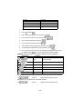
Introduction
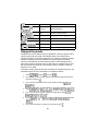
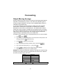
This Solutions Handbook has been designed to supplement the HP-12C
Owner's Handbook by providing a variety of applications in the financial
area. Programs and/or step-by-step keystroke procedures with
corresponding examples in each specific topic are explained. We hope
that this book will serve as a reference guide to many of your problems
and will show you how to redesign our examples to fit your specific needs.
1
Real Estate
Refinancing
It can be mutually advantageous to both borrower and lender to refinance
an existing mortgage which has an interest rate substantially below the
current market rate, with a loan at a below-market rate. The borrower has
the immediate use of tax-free cash, while the lender has substantially
increased debt service on a relatively small cash outlay.
To find the benefits to both borrower and lender:
1.
Calculate the monthly payment on the existing mortgage.
2.
Calculate the monthly payment on the new mortgage.
3.
Calculate the net monthly payment received by the lender (and paid by the
borrower) by adding the figure found in Step 1 to the figure found in Step 2.
4.
Calculate the Net Present Value (NPV) to the lender of the net cash
advanced.
5.
Calculate the yield to the lender as an IRR.
6.
Calculate the NPV to the borrower of the net cash received.
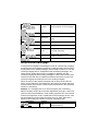
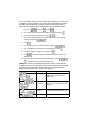
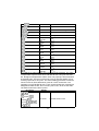
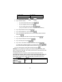
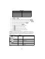
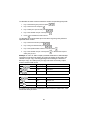
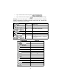
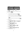
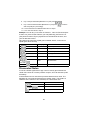
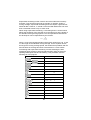
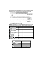
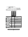
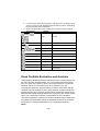
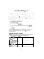
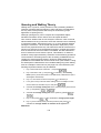
Example 1: An investment property has an existing mortgage which
originated 8 years ago with an original term of 25 years, fully amortized in
level monthly payments at 6.5% interest. The current balance is $133,190.
Although the going current market interest rate is 11.5%, the lender has
agreed to refinance the property with a $200,000, 17 year, level-monthlypayment loan at 9.5% interest.
What are the NPV and effective yield to the lender on the net abount of
cash actually advanced?
What is the NPV to the borrower on this amount if he can earn a 15.25%
equity yield rate on the net proceeds of the loan?
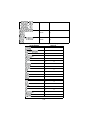
Keystrokes
Display
CLEAR
17
Monthly payment on existing
mortgage received by lender.
-1,080.33
6.5
133190
0
2
9.5
200000
0
133190
1,979.56
Monthly payment on new mortgage.
899.23
Net monthly payment (to lender).
-66,810.00
Net amount of cash advanced (by
lender).
-80,425.02
Present value of net
-13,615.02
NPV to lender of net cash advanced
14.83
% nominal yield (IRR).
-65,376.72
Present value of net monthly
payment at 15.25%.
1,433.28
NPV to borrower.
0
11.5
0
0
12
15.25
0
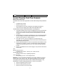
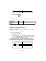
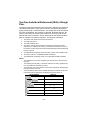
Wrap-Around Mortgage
A wrap-around mortgage is essentially the same as a refinancing mortgage,
except that the new mortgage is granted by a different lender, who assumes
the payments on the existing mortgage, which remains in full force. The new
(second) mortgage is thus “wrapped around” the existing mortgage. The
"wrap-around" lender advances the net difference between the new
(second) mortgage and the existing mortgage in cash to the borrower, and
receives as net cash flow, the difference between debt service on the new
(second) mortgage and debt service on the existing mortgage.
When the terms of the original mortgage and the wrap-around are the
same, the procedures in calculating NPV and IRR to the lender and NPV
to the borrower are exactly the same as those presented in the preceding
section on refinancing.
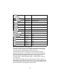
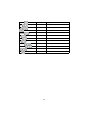
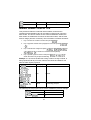
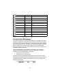
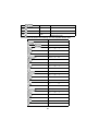
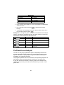
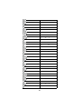
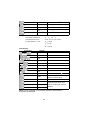
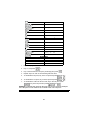
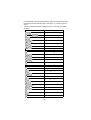
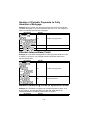
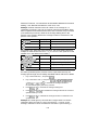
Example 1: A mortgage loan on an income property has a remaining
balance of $200,132.06. When the load originated 8 years ago, it had a 20year term with full amortization in level monthly payments at 6.75% interest.
A lender has agreed to “wrap” a $300,000 second mortgage at 10%, with
full amortization in level monthly payments over 12 years. What is the
effective yield (IRR) to the lender on the net cash advanced?
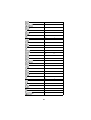
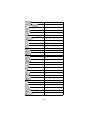
Keystrokes
Display
Total number of months remaining in
original load (into n).
144.00
3
CLEAR
20
8
6.75
0.56
Monthly interest rate (into i).
200132.06
200,132.06
Loan amount (into PV).
-2,031.55
Monthly payment on existing
mortgage (calculated).
10
0.83
Monthly interest on wrap-around.
300000
-300,000.00
Amount of wrap-around (into PV).
0
Monthly payment on wrap-around
(calculated).
Net monthly payment received (into
PMT).
3,585.23
0
1,553.69
-99,867.94
Net cash advanced (into PV).
15.85
Nominal yield (IRR) to lender
(calculated).
200132.06
12
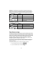
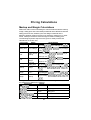
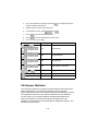
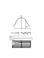
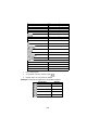
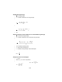
Sometimes the wrap around mortgage will have a longer payback period
than the original mortgage, or a balloon payment may exist.
where:
n1 = number of years remaining in original mortgage
PMT1 = yearly payment of original mortgage
PV1 = remaining balance of original mortgage
n2 = number of years in wrap-around mortgage
PMT2 = yearly payment of wrap-around mortgage
PV2 = total amount of wrap-around mortgage
BAL = balloon payment
4
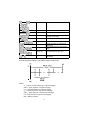
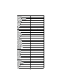
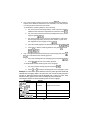
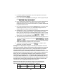
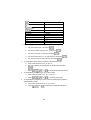
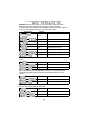
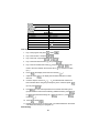
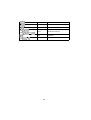
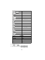
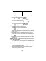
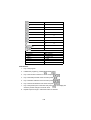
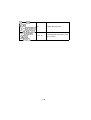
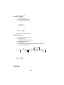
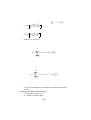
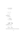
Example 2: A customer has an existing mortgage with a balance of
$125.010, a remaining term of 200 months, and a $1051.61 monthly
payment. He wishes to obtain a $200,000, 9 1/2% wrap-around with 240
monthly payments of $1681.71 and a balloon payment at the end of the
240th month of $129,963.35. If you, as a lender, accept the proposal, what
is your rate of return?
$125010
$129963.35
240 mos.
$1681.71
$1681.71
$-1051.61
$-1051.61
$1681.71
200mos.
$-200000
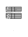
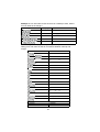
Keystrokes
CLEAR
Display
-74,990.00
Net investment.
630.10
Net cash flow received by lender.
200000
125010
1051.61
1681.71
99
The above cash flow occurs 200
times.
2
39
129963.35
12
1,681.71
Next cash flow received by lender.
39.00
Cash flow occurs 39 times.
131,645.06
Final cash flow.
11.84
Rate of return to lender.
5
If you, as a lender, know the yield on the entire transaction, and you wish
to obtain the payment amount on the wrap-around mortgage to achieve
this yield, use the following procedure. Once the monthly payment is
known, the borrower's periodic interest rate may also be determined.
1.
Press the
and press
CLEAR
2.
Key in the remaining periods of the original mortgage and press
3.
Key in the desired annual yield and press
4.
Key in the monthly payment to be made by the lender on the original
mortgage and press
.
.
.
.
5.
Press
.
6.
Key in the net amount of cash advanced and press
7.
Key in the total term of the wrap-around mortgage and press
8.
If a balloon payment exists, key it in and press
9.
Press
to obtain the payment amount necessary to achieve the
desired yield.
.
.
.
10. Key in the amount of the wrap-around mortgage and press
to obtain the borrower's periodic interest rate.
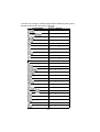
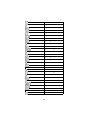
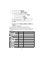
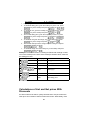
Example 3: Your firm has determined that the yield on a wrap-around
mortgage should be 12% annually. In the previous example, what monthly
payment must be received to achieve this yield on a $200,000 wraparound? What interest rate is the borrower paying?
Keystrokes
Display
Number of periods and monthly
interest rate.
CLEAR
200
12
1051.61
74990
240
-165,776.92
Present value of payments plus cash
advanced.
1,693.97
Monthly payment received by lender
9.58
Annual interest rate paid by borrower.
129963.35
2000
6
12
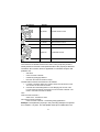
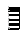
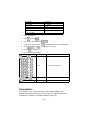
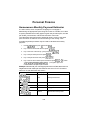
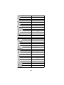
Income Property Cash Flow Analysis
Before-Tax Cash Flows
The before-tax cash flows applicable to real estate analysis and problems
are:
•
Potential Gross Income
•
Effective Gross Income
•
Net Operating Income (also called Net Income Before Recapture.)
•
Cash Throw-off to Equity (also called Gross Spendable Cash)
The derivation of these cash flows follows a set sequence:
1.
Calculate Potential Gross Income by multiplying the rent per unit times the
number of units, times the number of rental payments periods per year.
This gives the rental income the property would generate if it were fully
occupied.
2.
Deduct Allowance for Vacancy and Rental Loss. This is usually expressed
as a percentage. The result is Rent Collections (which is also Effective
Gross Income if there is no "Other Income").
3.
Add "Other Income" such as receipts from concessions (laundry
equipment, etc.), produced from sources other than the rental office space.
This is Effective Gross Income.
4.
Deduct Operating Expenses. These are expenditures the landlord-investor
must make, by contract or custom, to preserve the property and keep in
capable of producing the gross income. The result is the Net Operating
Income.
5.
Deduct Annual Debt Service on the mortgage. This produces Cash ThrowOff to Equity.
Thus:
Effective Gross Income =
Potential Gross Income - Vacancy Loss + Other Income.
Net Operating Income =
Effective Gross Income - Operating Expenses.
Cash Throw-Off =
Net Operating Income - Annual Dept Service.
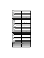
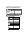
Example: A 60-unit apartment building has rentals of $250 per unit per
month. With a 5% vacancy rate, the annual operating cost is $76,855.
The property has just been financed with a $700,000 mortgage, fully
amortized in a level monthly payments at 11.5% over 20 years.
a.
What is the Effective Gross Income?
b.
What is the Net Operating Income?
c.
What is the Cash Throw-Off to Equity?
7
Keystrokes
CLEAR
Display
180,000.00
Potential Gross Income.
9,000.00
Vacancy Loss.
171,000.00
Effective Gross Income.
94,145.00
Net Operating Income.
-89,580.09
Annual Debt Service.
4,564.91
Cash Throw-Off.
60
250
12
5
76855
20
11.5
700000
12
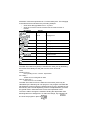
Before-Tax Reversions (Resale Proceeds)
The reversion receivable at the end of the income projection period is
usually based on forecast or anticipated resale of the property at that time.
The before tax reversion amount applicable to real estate analysis and
problems are:
•
Sale Price.
•
Cash Proceeds of Resale.
•
Outstanding Mortgage Balance.
•
Net Cash Proceeds of Resale to Equity.
The derivation of these reversions are as follows:
1.
Forecast or estimate Sales Price. Deduct sales and Transaction Costs.
The result is the Proceeds of Resale.
2.
Calculate the Outstanding Balance of the Mortgage at the end of the
Income Projection Period and subtract it from Proceeds of Resale. The
result is net Cash Proceeds of Resale.
Thus:
Cash Proceeds of Resale =
Sales Price - Transaction Costs.
Net Cash Proceeds of Resale =
Cash Proceeds of Resale - Outstanding Mortgage Balance.
Example: The apartment property in the preceding example is expected
to be resold in 10 years. The anticipated resale price is $800,000. The
8
transaction costs are expected to be 7% of the resale price. The mortgage
is the same as that indicated in the preceding example.
•
What will the Mortgage Balance be in 10 years?
•
What are the Cash Proceeds of Resale and Net Cash Proceeds of
Resale?
Keystrokes
Display
CLEAR
240.00
Mortgage term.
0.96
Mortgage rate.
20
11.5
Property value.
700000
10
-7,465.01
Monthly payment.
120.00
Projection period.
-530,956.57
Mortgage balance in 10 years.
Estimated resale.
800000
7
56,000.00
Transaction costs.
744,000.00
Cash Proceeds of Resale.
213,043.43
Net Cash Proceeds of Resale.
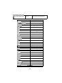
After-Tax Cash Flows
The After-Tax Cash Flow (ATCF) is found for the each year by deducting
the Income Tax Liability for that year from the Cash Throw Off.
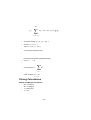
where:
Taxable Income =
Net Operating Income - interest - depreciation.
Tax Liability =
Taxable Income x Marginal Tax Rate.
After Tax Cash Flow =
Cash Throw Off - Tax Liability.
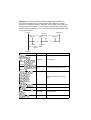
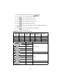
The After-Tax Cash Flow for the initial and successive years may be
calculated by the following HP-12C program. This program calculates the
Net Operating Income using the Potential Gross Income, operational cost
and vacancy rate. The Net Operating Income is readjusted each year from
the growth rates in Potential Gross Income and operational costs.
The user is able to change the method of finding the depreciation from
declining balance to straight line. To make the change, key in
.
line 32 of the program in place of
9
at
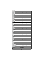
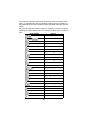
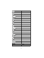
KEYSTROKES
CLEAR
0
DISPLAY
0001-
0
02-
11
1
03-
44
1
7
04-
45
7
2
05-
26
06-
2
07-
10
08-
7
1
44
091
1
2
10-44
7
1
40
1112-
1
1
2
13-
42
11
0
14-
44
0
5
15-
45
5
16-
6
6
11
17-
45
12
18-
45
6
19-
12
20-
33
21-
44
22-
4
6
33
23-
45
13
24-
45
4
25-
13
26-
33
10
27-
4
44
282936
1
0
0
33
43
35
30-43, 33
36
31-
45
1
32-
42
25
33-44
30
0
3417
4
0
35-43, 33
17
36-
11
2
37-
45
2
8
38-
45
8
392
40-44
25
40
410
42-45
2
33
48
0
43-
25
44-
30
3
45-
45
3
9
46-
45
9
473
1
7
0
48-44
25
40
3
49-
33
50-
30
51-
1
52-
45
7
53-44
20
0
54-
11
30
55-
20
561
2
45
5758-
1
2
59-
20
60-
40
61-
0
14
45
0
621
09
30
63-
45
1
64-
43
31
65-
34
66-
31
67-43, 33
09
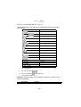
REGISTERS
i: Annual %
PMT: Monthly
R0: Used
R2: PGI
R4: Dep. value
R6: Factor (DB)
R8: % gr. (PGI)
R.0: Vacancy rt.
n: Used
PV: Used
FV: 0
R1: Counter
R3: Oper. cost
R5: Dep. life
R7: Tax Rate
R9: % gr. (op)
1.
Press
and press
2.
Key in loan values:
CLEAR
.
•
Key in annual interest rate and press
•
Key in principal to be paid and press
•
Key in monthly payment and press
(If any of the values are not known, they should be solved for.)
3.
Key in Potential Gross Income (PGI) and press
4.
Key in Operational cost and press
12
3.
2.
5.
Key in depreciable value and press
6.
Key in depreciable life and press
7.
Key in factor (for declining balance only) and press
8.
Key in the Marginal Tax Rate (as a percentage) and press
9.
Key in the growth rate in Potential Gross Income ( 0 for no growth) and
press
4.
5.
6.
7.
8.
10. Key in the growth rate in operational cost (0 if no growth) and press
9.
11. Key in the vacancy rate (0 for no vacancy rate) and press
0.
12. Key in the desired depreciation function at line 32 in the program.
13. Press
to compute ATCF. The display will pause showing the year
and then will stop with the ATCF for that year. The Y-register contains the
year.
14. Continue pressing
to compute successive After-Tax Cash Flows.
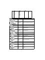
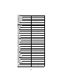
Example 1: A triplex was recently purchased for $100,000 with a 30-year
loan at 12.25% and a 20% down payment. Not including a 5% annual
vacancy rate, the potential gross income is $9,900 with an annual growth
rate of 6%. Operating expenses are $3,291.75 with a 2.5% growth rate. The
depreciable value is $75,000 with a projected useful life of $20 years.
Assuming a 125% declining balance depreciation, what are the After-Tax
Cash Flows for the first 10 years if the investors Marginal Tax Rate is 35%?
Keystrokes
CLEAR
Display
80,000.00
Mortgage amount.
12.25
1.02
Monthly interest rate.
30
360
Mortgage term.
-838.32
Monthly payment.
9,900.00
Potential Gross Income.
3,291.75
1st year operating cost.
75,000.00
Depreciable value.
20.00
Useful life.
100000
20
9900
2
3291.75
3
75000
20
4
5
13
125
6
35
7
6
8
2.5
9
5
.0
125.00
Decline in balance factor.
35.00
Marginal Tax Rate.
6.00
Potential Gross Income growth rate.
2.50
Operating cost growth.
5.00
Vacancy rate.
1.00
-1,020.88
2.00
-822.59
3.00
-598.85
4.00
-72.16
5.00
232.35
6.00
565.48
7.00
928.23
8.00
1,321.62
9.00
1,746.81
10.00
-1,020.88
Year 1
ATCF1
Year 2
ATCF2
Year 3
ATCF3
Year 4
ATCF4
Year 5
ATCF5
Year 6
ATCF6
Year 7
ATCF7
Year 8
ATCF8
Year 9
ATCF9
Year 10
ATCF10
Example 2: An office building was purchased for $1,400,000. The value
of depreciable improvements is $1,200,000.00 with a 35 year economic
life. Straight line depreciation will be used. The property is financed with a
$1,050,000 loan. The terms of the loan are 9.5% interest and $9,173.81
monthly payments for 25 years. The office building generates a Potential
Gross Income of $175,2000 which grows at a 3.5% annual rate. The
operating cost is $40,296.00 with a 1.6% annual growth rate. Assuming a
Marginal Tax Rate of 50% and a vacancy rate of 7%, what are the AfterTax Cash Flows for the first 5 years?
Keystrokes
Display
CLEAR
1050000
175,200.00
Potential Gross Income.
9173.81
9.5
14
25
175200
2
40296
3
1200000
4
40,296.00
1st year operating cost.
1,200,000.00
Depreciable value.
35
5
35.00
Depreciable life.
50
7
50.00
Marginal tax rate.
3.5
8
3.50
Potential Gross Income
1.6
9
1.60
Operating cost growth rate.
0
7.00
Vacancy rate.
31
7.00
Go to dep. step.
3242
23
1.00
18,021.07
2.00
20,014.26
3.00
22,048.90
4.00
24,123.14
5.00
26,234.69
Change to SL.
7
Year 1
ATCF1
Year 2
ATCF2
Year 3
ATCF3
Year 4
ATCF4
Year 5
ATCF5
After-Tax Net Cash Proceeds of Resale
The After-Tax Net Cash Proceeds of Resale (ATNCPR) is the after-tax
reversion to equity; generally, the estimated resale price of the property
less commissions, outstanding debt and any tax claim.
The After-Tax Net Cash Proceeds can be found using the HP-12C
program which follows. In calculating the owner's income tax liability on
resale, this program assumes that the owner elects to have his capital
gain taxed at 40% of his Marginal Tax Rate. This assumption is in
accordance with a 1978 Federal tax ruling.* (*Federal Taxes, code sec.
1202 (32,036))
This program uses declining balance depreciation to find the amount of
depreciation from purchase to sale. This amount is used to determine the
excess depreciation (which is equal to the amount of actual depreciation
minus the amount of the straight line depreciation).
15
The user may change to a different depreciation method by keying in the
desired function at line 35 in place of
.
KEYSTROKES
CLEAR
2
DISPLAY
0001-
43
8
02-
44
2
03-
33
04-
25
05-
30
06-
4
1
44
07-
30
08-
48
09-
4
10-
20
11-
44
1
12-
45
14
13-
42
14
142
0
14
15-
45
2
16-
43
11
17-
15
18-44
40
0
CLEAR
19-
42
34
3
20-
45
3
0
214
22-
13
45
235
24-
16
4
11
45
5
252
2
6
1
2
12
26-
45
2
27-
42
23
28-
45
2
29-
20
30-
48
31-
6
32-
20
33-44
40
1
34-
45
2
35-
42
25
3637-
34
45
381
6
2
30
39-44
40
1
40-
45
6
41-
26
42-
2
43-
10
44-
1
45
4546-
0
n: Used
PV: Used
FV: Used
R1: Used
48-43
45
0
40
33
REGISTERS
i: Used
PMT: Used
R0: Used
R2: Desired yr.
17
1
20
4700
13
00
R3: Dep. value
R5: Factor
R7-R.3: Unused
R4: Dep. life
R6: MTR
1.
Key in the program and press
2.
Key in the loan values:
CLEAR
.
•
Key in annual interest rate and press
•
Key in mortgage amount and press
•
Key in monthly payment and press
.
.
.
(If any of the values are unknown, they should be solved for.)
3.
Key in depreciable value and press
4.
Key in depreciable life in years and press
5.
Key in accelerated depreciation factor for the declining balance method
and press
3.
4.
5.
6.
Key in your Marginal Tax Rate as a percentage and press
7.
Key in the purchase price and press
8.
Key in the sale price and press
9.
Key in the % commission charged on the sale and press
6.
.
.
.*
*If a dollar value is desired instead of a commission rate, key in
which does not affect the register values, at line 04 of the program.
10. Key in the number of years after purchase and press
,
.
Example 1: An apartment complex, purchased for $900,000 ten years
ago, is sold for $1,750,000. The closing cost are 8% of the sale price and
the income tax rate is 48%.
A $700,000 loan for 20 years at 9.5% annual interest was used to
purchase the complex. When it was purchased the depreciable value was
$750,000 with a useful life of 25 years. Using 125% declining balance
depreciation, what are the After-Tax Net Cash Proceeds in year 10?
Keystrokes
Display
0.00
CLEAR
18
700000
700,000.00
Mortgage.
9.5
0.79
Monthly interest.
20
240.00
Number of payments.
-6,524.92
Monthly payment.
750,000.00
Depreciable value.
25.00
Depreciable life.
125.00
Factor.
48.00
Marginal Tax Rate.
900000
900,000.00
Purchase price.
1750000
1,750,000.00
Sale price.
8
8.00
Commission rate.
10
911,372.04
ATNCPR.
750000
25
125
48
3
4
5
6
19
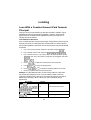
Lending
Loan With a Constant Amount Paid Towards
Principal
This type of loan is structured such that the principal is repaid in equal
installments with the interest paid in addition. Therefor each periodic
payment has a constant amount applied toward the principle and a
varying amount of interest.
Loan Reduction Schedule
If the constant periodic payment to principal, annual interest rate, and loan
amount are known, the total payment, interest portion of each payment,
and remaining balance after each successive payment may be calculated
as follows:
1.
Key in the constant periodic payment to principal and press
0.
2.
Key in periodic interest rate and press
3.
Key in the loan amount. If you wish to skip to another time period, press
.
. Then key in the number of payments to be skipped, and press
0
.
4.
Press
to obtain the interest portion of the payment.
5.
Press
6.
Press
7.
Return to step 4 for each successive payment.
0
to obtain the total payment.
0
to obtain the remaining balance of the loan.
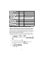
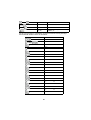
Example 1: A $60,000 land loan at 10% interest calls for equal semiannual principal payments over a 6-year maturity. What is the loan
reduction schedule for the first year? (Constant payment to principal is
$5000 semi-annually). What is the fourth year's schedule (skip 4
payments)?
Keystrokes
5000
0
10
2
60000
0
Display
5.00
Semi-annual interest rate.
3,000.00
First payment's interest.
8,000.00
Total first payment.
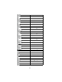
20
0
0
0
4
0
0
0
0
0
55,000.00
Remaining balance.
2,750.00
Second payment's interest.
7,750.00
Total second payment.
50,000.00
Remaining balance after the first
year.
1,500.00
Seventh payment's interest.
6,500.00
Total seventh payment.
25,000.00
Remaining balance.
1,250.00
Eighth payment's interest.
6,250.00
Total eighth payment.
20,000.00
Remaining balance after fourth
year.
Add-On Interest Rate Converted to APR
An add-on interest rate determines what portion of the principal will be
added on for repayment of a loan. This sum is then divided by the number
of months in a loan to determine the monthly payment. For example, a
10% add-on rate for 36 months on $3000 means add one-tenth of $3000
for 3 years (300 x 3) - usually called the "finance charge" - for a total of
$3900. The monthly payment is $3900/36.
This keystroke procedure converts an add-on interest rate to a annual
percentage rate when the add-on rate and number of months are known.
1.
Press
and press
CLEAR
.
2.
Key in the number of months in loan and press
.
3.
Key in the add-on rate and press
4.
Key in the amount of the loan and press
received; negative for cash paid out.)
5.
Press
6.
Press
.
12
to obtain the APR.
21
.
* (*Positive for cash
.
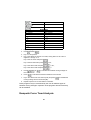
Example 1: Calculate the APR and monthly payment of a 12% $1000
add-on loan which has a life of 18 months.
Keystrokes
Display
CLEAR
18
1,180.00
Amount of loan.
-65.56
Monthly payment.
21.64
Annual Percentage Rate.
12
1000
12
APR Converted to Add-On Interest Rate.
Given the number of months and annual percentage rate, this procedure
calculates the corresponding add-on interest rate.
1.
Press
2.
Enter the following information:
3.
and press
CLEAR
.
a.
Key in number of months of loan and press
b.
Key in APR and press
c.
Key in 100 and press
.
.
.
Press
12
to obtain the add-on
rate.
Example 1: What is the equivalent add-on rate for an 18 month loan with
an APR of 14%.
Keystrokes
Display
CLEAR
18
14
7.63
Add-On Interest Rate.
100
12
22
Add-On Rate Loan with Credit Life.
This HP-12C program calculates the monthly payment amount, credit life
amount (an optional insurance which cancels any remaining indebtedness
at the death of the borrower), total finance charge, and annual percentage
rate (APR) for an add-on interest rate (AIR) loan. The monthly payment is
rounded (in normal manner) to the nearest cent. If other rounding
techniques are used, slightly different results may occur.
KEYSTROKES
CLEAR
DISPLAY
0001-
1
43
020
1
2
0
0
03-
8
1
45
0
04050607-
1
2
0
0
08-
10
4
09-
44
4
2
10-
45
2
1
11-
20
12-
30
13-
43
36
14-
45
1
154
16-
20
45
4
17-
20
18-
30
4
19-
45
4
1
20-
45
1
21-
23
20
1
3
22-
1
23-
40
24-
34
25-
10
26-
45
270
28-
20
45
2930-
0
2
1
2
5
2
0
10
42
14
31-
16
32-
14
33-
31
34-
45
14
35-
45
0
36-
20
37-
16
38-
13
39-
45
13
40-
45
2
410
3
42-
25
45
0
43-
20
4445-
1
2
46-
10
47-
44
5
48-
26
49-
2
50-
20
24
61
51-
43
35
52-
43
35
53-43, 33
61
54-
5
0
1
45
5
55-
48
5657-
0
1
58-
40
59-
42
14
5
60-
44
5
5
61-
45
5
6263-
45
13
64-
34
65-
30
66-
3
31
45
3
67-
30
68-
16
69-
31
5
70-
45
5
3
71-
45
3
72-
40
73-
13
74-
0
00
45
0
75-
11
76-
12
77-45, 43
12
78-43, 33
00
25
REGISTERS
i: i
PMT: PMT
R0: N
R2: CL (%)
R4: N/1200
R6-R9: Unused
n: N
PV: Used
FV: 0
R1: AIR
R3: Loan
R5: Used
1.
Key in the program.
2.
Press
3.
Key in the number of monthly payments in the loan and press
4.
Key in the annual add-on interest rate as a percentage and press
5.
Key in the credit life as a percentage and press
6.
Key in the loan amount and press
7.
Press
to find the monthly payment amount.
8.
Press
to obtain the amount of credit life.
9.
Press
to calculate the total finance charge.
CLEAR
10. Press
.
0.
1.
2.
3.
to calculate the annual percentage rate.
11. For a new loan return to step 3.
Example 1: You wish to quote a loan on a $3100 balance, payable over
36 months at an add-on rate of 6.75%. Credit life (CL) is 1%. What are the
monthly payment amount, credit life amount, total finance charge, and
APR?
Keystrokes
CLEAR
36
3100
36.00
Months.
6.75
Add-on interest rate.
1.00
Credit life (%).
3100.00
Loan.
-107.42
Monthly payment.
116.02
Credit life.
0
6.75
1
Display
1
2
3
26
-651.10
Total finance charge.
12.39
APR.
Interest Rebate - Rule of 78's
This procedure finds the unearned interest rebate, as well as the
remaining principal balance due for a prepaid consumer loan using the
Rule of 78's. The known values are the current installment number, the
total number of installments for which the loan was written, and the total
finance charge (amount of interest). The information is entered as follows:
1.
Key in number of months in the loan and press
2.
Key in payment number when prepayment occurs and press
1
3.
2
.
Key in total finance charge and press
2
4.
1.
1
1
to obtain the unearned interest (rebate).
Key in periodic payment amount and press
2
to
obtain the amount of principal outstanding.
Example 1: A 30 month $1000 loan having a finance charge of $180, is
being repaid at $39.33 per month. What is the rebate and balance due
after the 25th regular payment?
Keystrokes
30
1
25
1
Display
2
180
5.81
Rebate.
190.84
Outstanding principal.
1
1
2
39.33
2
The following HP-12C program can be used to evaluate the previous example.
KEYSTROKES
CLEAR
DISPLAY
00-
27
01-
0
44
0203-
2
0
33
44
04-
2
33
1
05-
44
1
2
06-
45
2
0708-
2
1
44
1
10-
40
45
1213-
1
00
n: Unused
45
1
15-
20
45
1
17-
40
18-
10
45
2
20-
20
21-
31
22-
2
20
36
19-
2
0
14-
16-
1
2
09-
11-
0
30
45
2
23-
20
24-
34
25-
30
26-43, 33
00
REGISTERS
i: Unused
28
PV: Unused
FV: Unused
R1: Payment#
R3-R.6: Unused
PMT: Unused
R0: Fin. charge
R2: # moths
1.
Key in the program.
2.
Key in the number of months in the loan and press
3.
Key in the payment number when prepayment occurs and press
.
.
4.
Key in the total finance charge and press
interest (rebate).
5.
Key in the periodic payment amount and press
principal outstanding.
6.
For a new case return to step 2.
Keystrokes
to obtain the unearned
to find the amount of
Display
30
25
5.81
Rebate.
190.84
Outstanding principal.
180
39.33
Graduated Payment Mortgages
The Graduated Payment Mortgage is designed to meet the needs of
young home buyers who currently cannot afford high mortgage payments,
but who have the potential of increasing earning in the years on come.
Under the Graduated Payment Mortgage plan, the payments increase by
a fixed percentage at the end of each year for a specified number of years.
Thereafter, the payment amount remains constant for remaining life of the
mortgage.
The result is that the borrower pays a reduced payment (a payment which
is less than a traditional mortgage payment) in the early years, and in the
later years makes larger payments than he would with a traditional loan.
Over the entire term of the mortgage, the borrower would pay more than
he would with conventional financing.
Given the term of the mortgage (in years), the annual percentage rate, the
loan amount, the percentage that the payments increase, and the number
of years that the payments increase, the following HP-12C program
determines the monthly payments and remaining balance for each year
until the level payment is reached.
29
KEYSTROKES
CLEAR
2
1
1
0
2
DISPLAY
0001-
43
8
02-
44
2
03-
34
04-
1
05-
25
06-
1
07-
40
08-
44
0
09-
45
11
10-
45
2
11-
3
1
1
30
12-
43
11
13-
45
12
14-
43
12
15-
45
13
16-
44
3
17-
1
18-
16
19-
14
20-
13
21-
16
22-
15
23-
0
1
24-
43
11
25-
45
14
26-
45
0
27-
30
10
1
1
28-
14
29-
13
30-
16
31-
15
32-
1
33-
1
1
34-44
40
1
2
35-
45
2
3637-
3
30
43
35
40
38-43, 33
40
25
39-43, 33
25
40-
45
3
41-
45
13
42-
10
4
43-
44
4
3
44-
45
3
451
13
46-
1
3
47-
44
3
3
48-
45
3
494
1
50-
31
45
51-
4
1
0
52-
45
0
1
53-
45
1
54-
21
55-
10
31
56-
20
57-
16
58-
14
60-
31
61-
15
62-
15
42
14
64-
31
65-
16
66-
13
67-
1
3
68-44
40
3
1
69-44
30
1
70-
45
1
71-
43
35
74
72-43, 33
74
48
73-43, 33
48
1
74-
4
76
n: Used
PV: Used
FV: Used
R1: Used
R3: Used
R5-R9: Unused
1.
14
59-
63-
1
42
45
4
75-
16
76-
31
77-43, 33
76
REGISTERS
i: i/12
PMT: Used
R0: Used
R2: Used
R4: Level Pmt.
Key in the program.
32
2.
Press
3.
Key in the term of the loan and press
4.
Key in the annual interest rate and press
.
5.
Key in the total loan amount and press
.
6.
Key in the rate of graduation (as a percent) and press
7.
Key in the number of years for which the loan graduates and press
The following information will be displayed for each year until a level
payment is reached.
a.
CLEAR
.
.
to continue.
The monthly payment for the current year.
Then press
c.
.
The current year.
Then press
b.
.
to continue.
The remaining balance to be paid on the loan at the end of the current year. Then press
to return to step a. unless the level
payment is reached. If the level payment has been reached, the
program will stop, displaying the monthly payment over the remaining term of the loan.
8.
For a new case press
00 and return to step 2.
Example: A young couple recently purchased a new house with a
Graduated Payment Mortgage. The loan is for $50,000 over a period of 30
years at an annual interest rate of 12.5%. The monthly payments will be
graduating at an annual rate of 5% for the first 5 years and then will be
level for the remaining 25 years. What are the monthly payment amount
for the first 6 years?
Keystrokes
CLEAR
Display
0.00
30
30.00
Term
12.5
12.50
Annual interest rate
50000
50,000.00
Loan amount
5
5.00
Rate of graduation
5
1.00
Year 1
-448.88
1st year monthly payment.
-50,194.67
Remaining balance after 1st year.
2.00
Year 2
33
-471.33
2nd year monthly payment.
-51,665.07
Remaining balance after 2nd year.
3.00
Year 3
-494.89
3rd year monthly payment.
-52,215.34
Remaining balance after 3rd year.
4.00
Year 4
-519.64
4th year monthly payment.
-52.523.34
Remaining balance after 4th year.
5.00
Year 5
-545.62
5th year monthly payment.
-52,542.97
Remaining balance after 5th year.
-572.90
Monthly payment for remainder of
term.
Variable Rate Mortgages
As its name suggests, a variable rate mortgage is a mortgage loan which
provides for adjustment of its interest rate as market interest rates change.
As a result, the current interest rate on a variable rate mortgage may differ
from its origination rate (i.e., the rate when the loan was made). This is the
difference between a variable rate mortgage and the standard fixed
payment mortgage, where the interest rate and the monthly payment are
constant throughout the term.
Under the agreement of the variable rate mortgage, the mortgage is
examined periodically to determine any rate adjustments. The rate
adjustment may be implemented in two ways:
1.
Adjusting the monthly payment.
2.
Modifying the term of the mortgage.
The period and limits to interest rate increases vary from state to state.
Each periodic adjustment may be calculated by using the HP-12C with the
following keystroke procedure. The original terms of the mortgage are
assumed to be known.
1.
Press
and press
CLEAR
34
.
2.
Key in the remaining balance of the loan and press
. The remaining
balance is the difference between the loan amount and the total principal
from the payments which have been made.
To calculate the remaining balance, do the following:
a.
Key in the previous remaining balance. If this is the first mortgage
adjustment, this value is the original amount of the loan. Press
b.
Key in the annual interest rate before the adjustment (as a percentage) and press
c.
.
.
Key in the number of years since the last adjustment. If this is the
first mortgage adjustment, then key in the number of years since
the origination of the mortgage. Press
.
d.
Key in the monthly payment over this period and press
e.
Press
.
to find the remaining balance, then press
CLEAR
.
3.
Key in the adjusted annual interest rate (as a percentage) and press
. To calculate the new monthly payment:
a.
Key in the remaining life of the mortgage (years) and press
b.
Press
.
to find the new monthly payment.
To calculate the revised remaining term of the mortgage:
c.
Key in the present monthly payment and press
d.
Press
12
.
to find the remaining term of the mortgage in years.
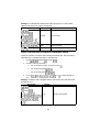
Example: A homeowner purchased his house 3 years ago with a $50,000
variable rate mortgage. With a 30-year term, his current monthly payment
is $495.15. When the interest rate is adjusted from 11.5% to 11.75%, what
will the monthly payment be? If the monthly payment remained
unchanged, find the revised remaining term on the mortgage.
Keystrokes
Display
50,000.00
Original amount of loan.
11.5
0.96
Original monthly interest rate.
3
36.00
Period.
495.15
-495.15
Previous monthly payment.
CLEAR
50000
35
-49,316.74
CLEAR
11.75
30
3
49,316.74
Remaining balance.
0.98
Adjusted monthly interest.
27.00
Remaining life of mortgage.
324.00
495.15
12
-504.35
New monthly payment.
-495.15
Previous monthly payment.
31.67
New remaining term (years).
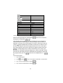
Skipped Payments
Sometimes a loan (or lease) may be negotiated in which a specific set of
monthly payments are going to be skipped each year. Seasonally is
usually the reason for such an agreement. For example, because of heavy
rainfall, a bulldozer cannot be operated in Oregon during December,
January, and February, and the lessee wishes to make payments only
when his machinery is being used. He will make nine payments per year,
but the interest will continue to accumulate over the months in which a
payment is not made.
To find the monthly payment amount necessary to amortize the loan in the
specified amount of time, information is entered as follows:
1.
Press
and press
2.
Key in the number of the last payment period before payments close the
first time and press
3.
CLEAR
.
.
Key in the annual interest rate as a percentage and press
1
.
4.
Press
12
0
5.
Key in the number of payments which are skipped and press
0
0
.
1
0.
6.
Press 0
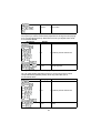
12
100
CLEAR
7.
Key in the total number of years in the loan and press
36
.
8.
Key in the loan amount and press
0
to obtain the
monthly payment amount when the payment is made at the end of the
month.
9.
Press
0
1
.
10. Key in the annual interest rate as a percent and press
find the monthly payment amount when the payment is made at the
beginning of the month.
to
Example: A bulldozer worth $100,000 is being purchased in September.
The first payment is due one month later, and payments will continue over
a period of 5 years. Due to the weather, the machinery will not be used
during the winter months, and the purchaser does not wish to make
payments during January, February, and March (months 4 thru 6). If the
current interest rate is 14%, what is the monthly payment necessary to
amortize the loan?
Keystrokes
Display
CLEAR
3.00
Number of payment made before a
group of payments is skipped.
3,119.98
Monthly payment in arrears.
3
14
1
12
0
0
3
1
0
0
0
12
100
CLEAR
5
100000
0
37
Savings
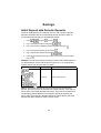
Initial Deposit with Periodic Deposits
Given an initial deposit into a savings account, and a series of periodic
deposits coincident with the compounding period, the future value (or
accumulated amount) may be calculated as follows:
1.
Press
and press
CLEAR
.
2.
Key in the initial investment and press
3.
Key in the number of additional periodic deposits and press
4.
Key in the periodic interest rate and press
5.
Key in the periodic deposit and press
6.
Press
.
.
.
.
to determine the value of the account at the end of the time
period.
Example: You have just opened a savings account with a $200 deposit. If
you deposit $50 a month, and the account earns 5 1/4 % compounded
monthly, how much will you have in 3 years?
Keystrokes
Display
CLEAR
200
2,178.94
Value of the account.
3
5.25
50
Note: If the periodic deposits do not coincide with the compounding
periods, the account must be evaluated in another manner. First, find the
future value of the initial deposits and store it. Then use the procedure for
compounding periods different from payment periods to calculate the
future value of the periodic deposits. Recall the future value of the initial
deposit and add to obtain the value of the account.
38
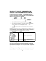
Number of Periods to Deplete a Savings
Account or to Reach a Specified Balance.
Given the current value of a savings account, the periodic interest rate,
the amount of the periodic withdrawal, and a specified balance, this
procedure determines the number of periods to reach that balance (the
balance is zero if the account is depleted).
1.
Press
and press
CLEAR
.
2.
Key in the value of the savings account and press
3.
Key in the periodic interest rate and press
4.
Key in the amount of the periodic withdrawal and press
5.
Key in the amount remaining in the account and press
.
.
.
. This step
may be omitted if the account is depleted (FV=0).
6.
Press
to determine the number of periods to reach the specified
balance.
Example: Your savings account presently contains $18,000 and earns 5
1/4% compounded monthly. You wish to withdraw $300 a month until the
account is depleted. How long will this take? If you wish to reduce the
account to $5,000, how many withdrawals can you make?
Keystrokes
Display
CLEAR
18000
71.00
Months to deplete account.
53.00
Months to reduce the account to
$5,000
5.25
300
5000
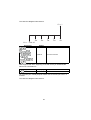
Periodic Deposits and Withdrawals
This section is presented as a guideline for evaluating a savings plan
when deposits and withdrawals occur at irregular intervals. One problem
is given, and a step by step method for setting up and solving the problem
is presented:
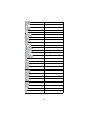
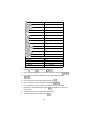
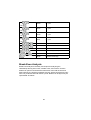
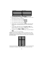
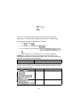
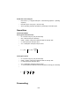
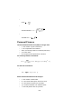
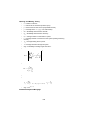
Example: You are presently depositing $50 and the end of each month into a
local savings and loan, earning 5 1/2% compounded monthly. Your current
balance is $1023.25. How much will you have accumulated in 5 months?
39
The cash flow diagram looks like this:
FV = ?
1
2
-50
3
-50
4
-50
5
-50
-50
PV = - 1023.25
Keystrokes
Display
CLEAR
50
1,299.22
Amount in account.
5.5
1023.25
5
Now suppose that at the beginning of the 6th month you withdrew $80.
What is the new balance?
Keystrokes
80
Display
1,219.22
New balance.
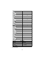
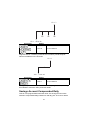
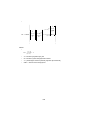
You increase your monthly deposit to $65. How much will you have in 3
months?
The cash flow diagram looks like this:
40
FV = ?
1
2
-65
3
-65
-65
PV = -1219.22
Keystrokes
Display
1,431.95
65
Account balance.
3
Suppose that for 2 months you decide not to make a periodic deposit.
What is the balance in the account?
FV = ?
1
2
PV = -1431.95
Keystrokes
2
Display
1,455.11
Account balance.
0
This type of procedure may be continued for any length of time, and may
be modified to meet the user's particular needs.
Savings Account Compounded Daily
This HP 12C program determines the value of a savings account when
interest is compounded daily, based on a 365 day year. The user is able to
41
calculate the total amount remaining in the account after a series of
transactions on specified dates.
KEYSTROKES
CLEAR
3
6
5
0
2
DISPLAY
0001-
16
02-
13
03-
33
040506-
3
6
5
07-
10
08-
12
09-
33
10-
44
0
11-
15
13
12-
16
13-
31
14-
44
15-
2
33
1
16-
44
1
0
17-
45
0
1
18-
45
1
19-
43
26
20-
11
21-
15
22-
42
14
23-
15
24-
36
25-
42
45
13
263
2
40
27-44
40
3
28-
45
15
29-
45
2
30-
40
31-
16
32-
13
1
33-
45
1
0
34-
44
0
35-
45
13
13
n: ∆days
PV: Used
FV: Used
R1: Next date
R3: Interest
36-
16
37-43, 33
13
REGISTERS
i: i/365
PMT: 0
R0: Initial date
R2: $ amount
R4-R.4: Unused
1.
Key in the program
2.
Press
3.
Key in the date (MM.DDYYYY) of the first transaction and press
4.
Key in the annual nominal interest rate as a percentage and press
CLEAR
and press
.
.
5.
Key in the amount of the initial deposit and press
6.
Key in the date of the next transaction and press
7.
Key in the amount of the transaction (positive for money deposited,
negative for cash withdrawn) and press
the account.
.
to determine the amount in
8.
Repeat steps 6 and 7 for subsequent transactions.
9.
To see the total interest to date, press
43
.
3.
.
10. For a new case press
and go to step 2.
Example: Compute the amount remaining in this 5.25% account after the
following transactions:
1.
January 19, 1981 deposit $125.00
2.
February 24, 1981 deposit $60.00
3.
March 16, 1981 deposit $70.00
4.
April 6, 1981 withdraw $50.00
5.
June 1, 1981 deposit $175.00
6.
July 6, 1981 withdraw $100.00
Keystrokes
Display
CLEAR
1.191981
125.00
Initial Deposit.
185.65
Balance in account, February 24,
1981.
256.18
Balance in account, March 16, 1981.
206.95
Balance in account, April 6 1981.
383.62
Balance in account, June 1, 1981.
285.56
Balance in account, July 6, 1981.
5.56
Total interest.
5.25
125
2.241981
60
3.161981
70
4.061981
50
6.0111981
175
7.061981
100
3
Compounding Periods Different From
Payment Periods
In financial calculations involving a series of payments equally spaced in
time with periodic compounding, both periods of time are normally equal
and coincident. This assumption is preprogrammed into the HP 12C.
44
I savings plans however, money may become available for deposit or
investment at a frequency different from the compounding frequencies
offered. The HP 12C can easily be used in these calculations. However,
because of the assumptions mentioned the periodic interest rate must be
adjusted to correspond to an equivalent rate for the payment period.
Payments deposited for a partial compounding period will accrue simple
interest for the remainder of the compounding period. This is often the
case, but may not be true for all institutions.
These procedures present solutions for future value, payment amount,
and number of payments. In addition, it should be noted that only annuity
due (payments at the beginning of payment period) calculations are
shown since this is the most common in savings plan calculations.
To calculate the equivalent payment period interest rate, information is
entered as follows:
1.
Press
2.
Key in the annual interest rate (as a percent) and press
3.
Key in the number of compounding periods per year and press
4.
Key in 100 and press
5.
Key in the number of payments (deposits) per year and press
CLEAR
and press
CLEAR
.
.
.
.
The interest rate which corresponds to the payment period is now in
register "i" and you are ready to proceed.
Example 1: Solving for future value.
Starting today you make monthly deposits of $25 into an account paying
5% compounded daily (365-day basis). At the end of 7 years, how much
will you receive from the account?
Keystrokes
Display
CLEAR
5
365
0.42
Equivalent periodic interest rate.
100
12
CLEAR
45
.
7
2,519.61
25
Future value.
Example 2: Solving for payment amount.
For 8 years you wish to make weekly deposits in a savings account paying
5.5% compounded quarterly. What amount must you deposit each week
to accumulate $6000.
Keystrokes
Display
CLEAR
5.5
4
0.11
Equivalent periodic interest rate.
-11.49
Periodic payment.
100
52
CLEAR
8
52
6000
Example 3: Solving for number of payment periods.
You can make weekly deposits of $10 in to an account paying 5.25%
compounded daily (365-day basis). How long will it take you to
accumulate $1000?
Keystrokes
Display
CLEAR
5.25
365
0.10
Equivalent periodic interest rate.
96.00
Weeks.
100
52
CLEAR
8
1000
46
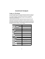
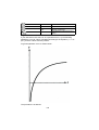
Investment Analysis
Lease vs. Purchase
An investment decision frequently encountered is the decision to lease or
purchase capital equipment or buildings. Although a thorough evaluation
of a complex acquisition usually requires the services of a qualified
accountant, it is possible to simplify a number of the assumptions to
produce a first approximation.
The following HP-12C program assumes that the purchase is financed
with a loan and that the loan is made for the term of the lease. The tax
advantages of interest paid, depreciation, and the investment credit which
accrues from ownership are compared to the tax advantage of treating the
lease payment as an expense. The resulting cash flows are discounted to
the present at the firm's after-tax cost of capital.
KEYSTROKES
CLEAR
1
0
3
8
1
DISPLAY
0001-
30
02-
1
03-44
40
0
04-
45
3
05-
30
06-
20
07-
44
08-
1
9
8
1
09-
42
11
10-
44
1
11-
45
13
12-
44
9
13-
45
14
14-44
48
0
47
1
2
5
15-
45
11
16-44
48
1
17-
45
12
18-44
48
2
19-
45
5
2021-
6
13
45
2223-
7
11
45
240
1
9
25-
45
0
26-
42
24
27-44
40
1
28-
45
9
30-45
13
48
311
32-45
34-45
0
14
48
332
7
12
290
6
1
11
48
35-
2
12
1
36-
45
1
3
37-
45
3
3839-
20
45
408
4142-
48
14
30
45
8
30
4
43-
45
4
0
44-
45
0
45-
21
46-
10
2
47-44
40
2
00
48-43, 33
00
REGISTERS
i: Used
PMT: Used
R0: Used
R2: Purch. Adv.
R4: Discount
R6: Dep. life
R8: Used
R.0: Used
R.2: Used
n: Used
PV: Used
FV: 0
R1: Used
R3: Tax
R5: Dep. Value
R7: Factor (DB)
R9: Used
R.1: Used
R.3: Unused
Instructions:
1.
Key in the program.
-Select the depreciation function and key in at line 26.
2.
Press
3.
Input the following information for the purchase of the loan:
and press
CLEAR
.
-Key in the number of years for amortization and press
-Key in the annual interest rate and press
.
.
-Key in the loan amount (purchase price) and press
-Press
.
to find the annual payment.
4.
Key in the marginal effective tax rate (as a decimal) and press
5.
Key in the discount rate (as a decimal) or cost of capital and press
1
4.
6.
Key in the depreciable value and press
7.
Key in the depreciable live and press
49
5.
6.
3.
8.
For declining balance depreciation, key in the depreciation factor (as a
percentage) and press
9.
7.
Key in the total first lease payment (including any advance payments) and
press
1
3
2.
10. Key in the first year's maintenance expense that would be anticipated if the
asset was owned and press . If the lease contract does not include
maintenance, then it is not a factor in the lease vs. purchase decision and
0 expense should be used.
11. Key in the next lease payment and press
. During any year in which
a lease payment does not occur (e.g. the last several payments of an
advance payment contract) use 0 for the payment.
12. Repeat steps 10 and 11 for all maintenance expenses and lease payments
over the term of the analysis. Optional - If the investment tax credit is
taken, key in the amount of the credit after finishing steps 10 and 11 for the
year in which the credit is taken and press
43
. Continue
steps 10 and 11 for the remainder of the term.
13. After all the lease payments and expenses have been entered (steps 10 and
11), key in the lease buy back option and press
43
1
3
. If no buy back option exists, use the estimated salvage
value of the purchased equipment at the end of the term.
14. To find the net advantage of owning press
2. A negative value
represents a net lease advantage.
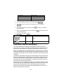
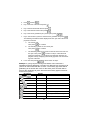
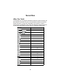
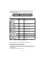
Example: Home Style Bagel Company is evaluating the acquisition of a mixer
which can be leased for $1700 a year with the first and last payments in advance
and a $750 buy back option at the end of 10 years (maintenance is included).
The same equipment could be purchased for $10,000 with a 12% loan
amortized over 10 years. Ownership maintenance is estimated to be 2% of the
purchase price per year for the first for years. A major overhaul is predicted for
the 5th year at a cost of $1500. Subsequent yearly maintenance of 3% is
estimated for the remainder of the 10-year term. The company would use sum
of the years digits depreciation on a 10 year life with $1500 salvage value. An
accountant informs management to take the 10% capital investment tax credit
at the end of the second year and to figure the cash flows at a 48% tax rate.
The after tax cost of capital (discounting rate) is 5 percent.
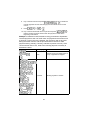
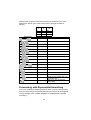
Because lease payments are made in advance and standard loan
payments are made in arrears the following cash flow schedule is
appropriate for a lease with the last payment in advance.
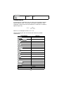
Year Maintenance Lease Payment Tax Credit Buy Back
0
1700+700
1
200
1700
50
2
3
4
5
6
7
8
9
10
200
200
200
1500
300
300
300
300
300
Keystrokes
1700
1700
1700
1700
1700
1700
1700
0
0
1000
750
Display
0.00
CLEAR
10
12
-10,000.00
Always use negative loan amount.
1,769.84
Purchase payment.
0.48
Marginal tax rate.
1.05
Discounting factor.
8,500.00
Depreciable value.
10.00
Depreciable life.
3,400.00
1st lease payment.
2 1,768.00
After-tax expense.
10000
.48
3
.05
1
4
10000
1500
5
10
6
1700
1
3
200
312.36
Present value of 1st year's net
purchase.
200.43
2nd year's advantage.
1,000.00
Tax credit.
907.03
Present value of tax credit.
95.05
3rd year.
-4.38
4th year.
1700
200
1700
1000
200
43
1700
200
1700
51
200
-628.09
5th year.
-226.44
6th year.
-309.48
7th year.
-388.81
8th year.
1700
200
1700
200
1700
200
1700
300
0
-1,034.72
9th year.
300
0
-1,080.88
10th year.
750.00
Buy back.
390.00
After tax buy back expense.
239.43
Present value.
-150.49
Net lease advantage.
750
1
3
43
2
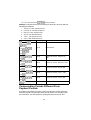
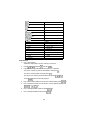
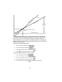
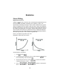
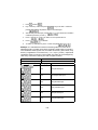
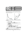
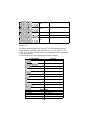
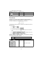
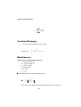
Break-Even Analysis
Break-even analysis is basically a technique for analyzing the
relationships among fixed costs, variable costs, and income. Until the
break even point is reached at the intersection of the total income and
total cost lines, the producer operates at a loss. After the break-even point
each unit produced and sold makes a profit. Break even analysis may be
represented as follows.
52
Sa
l
es
R
ev
u
en
Profit
e
To
Co
tal
sts
Variable
Costs
$
Break-Even Point
Lo
ss
Fixed Costs
The variables are: fixed costs (F), Sales price per unit (P), variable cost
per unit (V), number of units sold (U), and gross profit (GP). One can
readily evaluate GP, U or P given the four other variables. To calculate the
break-even volume, simply let the gross profit equal zero and calculate the
number of units sold (U).
To calculate the break-even volume:
1.
Key in the fixed costs and press
.
2.
Key in the unit price and press
3.
Key in the variable cost per unit and press
4.
Press
.
.
to calculate the break-even volume.
To calculate the gross profit at a given volume:
1.
Key in the unit price and press
.
2.
Key in the variable cost per unit and press
.
3.
Key in the number of units sold and press
.
4.
Key in the fixed cost and press
to calculate the gross profit.
53
To calculate the sales volume needed to achieve a specified gross profit:
1.
Key in the desired gross profit and press
2.
Key in the fixed cost and press
3.
Key in sales price per unit and press
4.
Key in the variable cost per unit and press
5.
Press
.
.
.
.
to calculate the sales volume.
To calculate the required sales price to achieve a given gross profit at a
specified sales volume:
1.
Key in the fixed costs and press
.
2.
Key in the gross desired and press
3.
Key in the specified sales volume in units and press
4.
Key in the variable cost per unit and press
.
.
to calculate the required
sales price per unit.
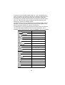
Example 1: The E.Z. Sells company markets textbooks on salesmanship.
The fixed cost involved in setting up to print the books are $12,000. The
variable cost per copy, including printing and marketing the books are
$6.75 per copy. The sales price per copy is $13.00. How many copies
must be sold to break even?
Keystrokes
Display
12000
12,000.00
Fixed cost.
13
13.00
Sales price.
6.75
1,920.00
Break-even volume.
Find the gross profit if 2500 units are sold.
13
13.00
Sales price.
6.75
6.25
Profit per unit.
2500
15,625.00
12000
3,625.00
Gross profit.
If a gross profit of $4,500 is desired at a sales volume of 2500 units, what
should the sales price be?
54
12000
12,000.00
4500
16,500.00
2500
6.60
6.75
13.35
Fixed cost.
Sales price per unit to achieve
desired gross profit.
For repeated calculation the following HP-12C program can be used.
KEYSTROKES
DISPLAY
CLEAR
00-
3
01-
45
3
2
02-
45
2
00
03-
30
04-43, 33
00
05-
4
45
0607-
1
00
4
20
45
1
08-
30
09-43, 33
00
5
10-
45
5
1
11-
45
1
00
12-
40
13-
34
14-
10
15-43, 33
00
1
16-
45
1
5
17-
45
5
184
1920-
55
40
45
4
10
21-
2
00
2.
2
22-
40
23-43, 33
00
REGISTERS
i: Unused
PMT: Unused
R0: Unused
R2: V
R4: U
R6-R.6: Unused
n: Unused
PV: Unused
FV: Unused
R1: F
R3: P
R5: GP
1.
45
Key in the program and store the know variables as follows:
a.
Key in the fixed costs, F and press
1.
b.
Key in the variable costs per unit, V and press
c.
Key in the unit price, P (if known) and press
d.
Key in the sales volume, U, in units (if known) and press
e.
Key in the gross profit, GP, (if known) and press
2.
3.
4.
5.
To calculate the sales volume to achieve a desired gross profit:
a.
Store values as shown in 1a, 1b, and 1c.
b.
Key in the desired gross profit (zero for break even) and press
5.
c.
3.
4.
Press
10
to calculate the required volume.
To calculate the gross profit at a given sales volume.
a.
Store values as shown in 1a, 1b, 1c, and 1d.
b.
Press
05
to calculate gross profit.
To calculate the sales price per unit to achieve a desired gross profit at a
specified sales volume:
a.
Store values as shown in 1a, 1b, 1d, and 1e.
b.
Press
16
to calculate the required sales price.
56
Example 2: A manufacturer of automotive accessories produces rear
view mirrors. A new line of mirrors will require fixed costs of $35,00 to
produce. Each mirror has a variable cost of $8.25. The price of mirrors is
tentatively set at $12.50 each. What volume is needed to break even?
Keystrokes
35000
1
Display
35,000.00
Fixed cost.
8.25
2
8.25
Variable cost.
12.5
3
12.50
Sales price.
0
0.00
5
10
Break-even volume is between 8,235
and 8,236 units.
8,235.29
What would be the gross profit if the price is raised to $14.00 and the
sales volume is 10,000 units?
Keystrokes
14
Display
14.00
3
Sales price.
F and V are already stored.
10000
4
05
10,000.00
Volume.
22,500.00
Gross Profit.
Operating Leverage
The degree of operating leverage (OL) at a point is defined as the ratio of
the percentage change in net operating income to the percentage change
in units sold. The greatest degree of operating leverage is found near the
break even point where a small change in sales may produce a very large
increase in profits. Likewise, firms with a small degree of operating
leverage are operating farther form the break even point, and they are
relatively insensitive to changes in sales volume.
The necessary inputs to calculate the degree of operating leverage and
fixed costs (F), sales price per unit (P), variable cost per unit (V) and
number of units (U).
The operating leverage may be readily calculated as follows:
1.
Key in the sales price per unit and press
2.
Key in the variable cost per unit and press
57
.
.
3.
Key in the number of units and press
4.
Key in the fixed cost and press
.
to obtain the operating leverage.
Example 1: For the data given in example 1 of the Break-Even Analysis
section, calculate the operating leverage at 2000 units and at 5000 units
when the sales price is $13 a copy
Keystrokes
Display
13
13.00
Price per copy.
6.75
6.25
Profit per copy.
25.00
Close to break-even point.
13
13.00
Price per copy.
6.75
6.25
Profit per copy.
1.62
Operating further from the breakeven
point and lesssensitive to changes in
sales volume.
2000
12000
5000
12000
For repeated calculations the following HP-12C program can be used:
KEYSTROKES
DISPLAY
CLEAR
00-
3
01-
45
3
2
02-
45
2
03-
30
04-
20
05-
36
06-
36
07-
1
00
45
1
08-
30
09-
10
10-43, 33
00
58
REGISTERS
i: Unused
PMT: Unused
R0: Unused
R2: V
R4-R.8: Unused
n: Unused
PV: Unused
FV: Unused
R1: F
R3: P
1.
Key in the program.
2.
Key in and store input variables F, V and P as described in the Break-Even
Analysis program.
3.
Key in the sales volume and press
to calculate the operating
leverage.
4.
To calculate a new operating leverage at a different sales volume, key in
the new sales volume and press
Example 2: For the figures given in example 2 of the Break-Even Analysis
section, calculate the operating leverage at a sales volume of 9,000 and
20,000 units if the sales price is $12.50 per unit.
Keystrokes
35000
1
Display
35,000.00
Fixed costs.
8.25
2
8.25
Variable cost.
12.5
3
12.50
Sales price.
9000
11.77
Operating leverage near break-even.
20000
1.70
Operating leverage further from
break-even.
Profit and Loss Analysis
The HP-12C may be programmed to perform simplified profit and loss
analysis using the standard profit income formula and can be used as a
dynamic simulator to quickly explore ranges of variables affecting the
profitability of a marketing operation.
The program operates with net income return and operating expenses as
percentages. Both percentage figures are based on net sales price.
It may also be used to simulate a company wide income statement by
replacing list price with gross sales and manufacturing cost with cost of
goods sold.
59
Any of the five variables: a) list price, b) discount (as a percentage of list
price), c) manufacturing cost, d) operating expense (as a percentage), e)
net profit after tax (as a percentage) may be calculated if the other four are
known.
Since the tax rage varies from company to company, provision is made for
inputting your applicable tax rate. The example problem uses a tax rate of
48%.
KEYSTROKES
DISPLAY
CLEAR
00-
5
01-
45
5
6
02-
45
6
0304-
4
45
40
06-
16
45
0809-
0
00
1
4
05-
07-
0
10
0
40
45
0
10-
10
11-43, 33
00
3
12-
45
3
1
13-
45
1
2
14-
45
2
0
15-
45
0
16-
10
17-
16
18-
1
19-
40
20-
20
21-
31
22-
10
60
1
23-
16
24-
1
25-
40
26-
0
45
2700
20
28-43, 33
10
30-
16
45
3233-
1
35-
00
1
40
45
340
0
29-
31-
1
0
1
10
45
0
36-
20
37-43, 33
00
5
38-
45
5
6
39-
45
6
00
40-
10
41-
30
42-43, 33
00
43-
4
45
4445-
6
00
n: Unused
PV: Unused
5
30
45
6
46-
20
47-43, 33
00
REGISTERS
i: Unused
PMT: Unused
61
R0: 100
R2: % discount
R4: % op. exp.
R6: 1-% tax
FV: Unused
R1: list price
R3: mfg. cost
R5: % net profit
R7-R.3: Unused
1.
Key in the program and press
press
2.
CLEAR
, then key in 100 and
0.
Key in 1 and press
, then key in your appropriate tax rate as a
decimal and press
6.
3.
a.
Key in the list price in dollars (if known) and press
1.
b.
Key in the discount in percent (if known) and press
c.
Key in the manufacturing cost in dollars (if known) and press
3.
d.
Key in the operating expense in percent (if known) and press
2.
4.
e.
4.
5.
6.
7.
8.
Key in the net profit after tax in percent (if known) and press
5.
To calculate list price:
a.
Do steps 2 and 3b, c, d, e above.
b.
Press
3
1
14
00.
To calculate discount:
a.
Do steps 2 and 3a, c, d, e above.
b.
Press
3
29
.
To calculate manufacturing cost:
a.
Do steps 2 and 3a, b, d, e, above.
b.
Press
13
01
.
To calculate operating expense:
a.
Do steps 2 and 3a, b, c, e, above.
b.
Press
12
38
To calculate net profit after tax:
a.
Do steps 2 and 3a, b, c, d, above.
62
.
b.
Press
12
43
.
Example: What is the net return on an item that is sold for $11.98,
discounted through distribution an average of 35% and has a
manufacturing cost of $2.50? The standard company operating expense
is 32% of net shipping (sales) price and tax rate is 48%.
Keystrokes
CLEAR
Display
100.00
100
0
1
.48
11.98
1
35
2
2.50
3
32
4
6 0.52
48% tax rate.
11.98
List price ($).
35.00
Discount (%).
2.50
Manufacturing cost ($).
32.00
Operating expenses (%).
12
67.90
43
18.67
Net profit (%).
If manufacturing expenses increase to $3.25, what is the effect on net
profit?
3
3.25
12
58.26
43
13.66
3.25
Manufacturing cost.
Net profit reduced to 13.66%
If the manufacturing cost is maintained at $3.25, how high could the
overhead (operating expense) be before the product begins to lose
money?
0
0.00
5
12
58.26
38
58.26
Maximum operating expense (%).
At 32% operating expense and $3.25 manufacturing cost, what should the
list price be to generate 20% net profit?
20
20.00
5
11.00
3
1
14
16.93
List price ($).
63
What reduction in manufacturing cost would achieve the same result
without necessitating an increase in list price above $11.98?
13
7.79
01
2.30
Manufacturing cost ($).
64
Securities
After-Tax Yield
The following HP-12C program calculate the after tax yield to maturity of a
bond held for more than one year. The calculations assumes an actual/
actual day basis. For after-tax computations, the interest or coupon
payments are considered income, while the difference between the bond
or note face value and its purchase price is considered capital gains.
KEYSTROKES
DISPLAY
CLEAR
00-
CLEAR
01-
42
34
7
02-
44
7
03-
33
6
04-
44
6
2
05-
45
2
1
06-
45
1
074
08-
30
45
092
2
10-
4
25
45
2
11-
34
12-
30
13-
26
14-
2
15-
10
0
16-
44
0
3
17-
45
3
5
18-
45
5
65
19-
25
20-
30
21-
0
45
0
22-
10
23-
14
1
24-
45
1
0
25-
45
0
26-
10
27-
13
6
28-
45
6
7
29-
45
7
30-
42
22
31-43, 33
00
00
n: Unused
PV: Used
FV: 0
R1: Purchase price
R3: Coupon rate
R5: Income rate
R7: Used
REGISTERS
i: Yield
PMT: Used
R0: Used
R2: Sales price
R4: Capital rate
R6: Used
R8-R.5: Unused
1.
Key in the program.
2.
Key in the purchase price and press
3.
Key in the sales price and press
4.
Key in the annual coupon rate (as a percentage) and press
5.
Key in capital gains tax rate (as a percentage) and press
6.
Key in the income tax rate (as a percentage) and press
7.
Press
.
66
1.
2.
3.
4.
5.
8.
Key in the purchase date (MM.DDYYYY) and press
.
9.
Key in the assumed sell date (MM.DDYYYY) and press
to find the
after-tax yield (as a percentage).
10. For the same bond but different date return to step 8.
11. For a new case return to step 2.
Example: You can buy a 7% bond on October 1, 1981 for $70 and expect
to sell it in 5 years for $90. What is your net (after-tax) yield over the 5year period if interim coupon payments are considered as income, and
your tax bracket is 50%?
(One-half of the long term capital gain is taxable at 50%, so the tax on
capital gains alone is 25%)
Keystrokes
Display
70
1
10.00
90
2
90.00
Selling price.
7.00
Annual coupon rate.
7
3
Purchase price.
25
4
25.00
Capital gains tax rate.
50
5
50.00
Income tax rate.
10.01
Purchase Date.
8.53
% after tax yield.
10.011981
10.011986
Discounted Notes
A note is a written agreement to pay a sum of money plus interest at a
certain rate. Notes to not have periodic coupons, since all interest is paid
at maturity.
A discounted note is a note that is purchase below its face value. The
following HP 12C program finds the price and/or yield* (*The yield is a
reflection of the return on an investment) of a discounted note.
KEYSTROKES
DISPLAY
CLEAR
00-
1
01-
67
45
1
2
3
02-
45
2
03-
43
26
04-
45
3
0506-
5
1
45
25
08-
1
09-
34
10-
30
45
1213-
5
5
07-
11-
4
10
4
20
44
14-
5
31
1
15-
45
1
2
16-
45
2
17-
43
26
18-
45
3
3
19-
34
20-
10
4
21-
45
4
5
22-
45
5
1
2
00
23-
10
24-
1
25-
30
26-
20
27-
26
28-
2
29-
20
30-43, 33
00
68
REGISTERS
i: Unused
PMT: Unused
R0: Unused
R2: Mat. date
R4: redemp. value
R6-R.5: Unused
n: Unused
PV: Unused
FV: Unused
R1: Settl. date
R3: 360 or 360
R5: dis./price
1.
Key in the program.
2.
Press
3.
Key in the settlement date (MM.DDYYYY) and press
4.
Key in the maturity date (MM.DDYYYY) and press
5.
Key in the number of days in a year (360 or 365) and press
6.
Key in the redemption value per $100 and press
7.
To calculate the purchase price:
8.
.
1.
2.
3.
4.
a.
Key in the discount rate and press
5.
b.
Press
to calculate the purchase price.
c.
Press
to calculate the yield.
d.
For a new case, go to step 3.
To calculate the yield when the price is known:
a.
Key in the price and press
b.
Press
c.
For a new case, go to step 3.
15
5.
to calculate the yield.
Example 1: Calculate the price and yield on this U.S. Treasury Bill:
settlement date October 8, 1980; maturity date March 21, 1981; discount
rate 7.80%. Compute on a 360 day basis.
Keystrokes
Display
10.08
10.081920
Settlement date.
1
69
3.211981
2
3.21
Maturity dtae.
360
3
360.00
360 day basis.
100
4
100.00
Redemption value per $100.
7.8
5
7.80
Discount rate.
96.45
Price.
8.09
Yield.
Example 2: Determine the yield of this security; settlement date June 25,
1980; maturity date September 10, 1980; price $99.45; redemption value
$101.33. Assume 360 day basis.
Keystrokes
Display
6.251980
1
6.25
Settlement date.
9.101980
2
9.10
Maturity dtae.
360.00
360 day basis.
101.33
Redemption value per $100.
99.45
Price.
8.84
Yield.
360
3
101.33
99.45
4
5
15
70
Forecasting
Simple Moving Average
Moving averages are often useful in recording of forecasting sales figures,
expenses or manufacturing volume. There are many different types of
moving average calculations. An often used, straightforward method of
calculation is presented here.
In a moving average a specified number of data points are averaged.
When there is a new piece of input data, the oldest piece of data is
discarded to make room for the latest input. This replacement scheme
makes the moving average a valuable tool in following trends. The fewer
the number of data points, the more trend sensitive the average becomes.
With a large number of data points, the average behaves more like a
regular average, responding slowly to new input data.
A simple moving average may be calculated with your HP 12C as follows.
1.
Press
CLEAR
2.
Key in the first m data points (where m is the number of data points in the
average) and press
.
after each entry.
3.
Press
to obtain the first average.
4.
Key in the oldest (first value) entered in step 2 and press
5.
Key in the newest data point (m + 1) and press
6.
Press
7.
Repeat steps 4 through 5 for the remaining data.
.
.
to obtain the next value of the moving average.
Example: An electronics sales firm wished to calculate a 3-month moving
average for the dollar volume of components sole each month. Sales for
the first six months of this year were:
January
February
March
April
May
June
Keystrokes
$211,570
112,550
190,060
131,760
300,500
271,120
Display
71
0.00
CLEAR
211570
1.00
112550
2.00
190060
3.00
171,393.33
211570
2.00
131760
3.00
3-month average for March.
144,790.00
112550
2.00
300500
3.00
3-month average for April.
207,440.00
190060
2.00
271120
3.00
3-month average for May.
234,460.00
3-month average for June.
For repeated calculations the following HP 12C program can be used for
up to a 12 element moving average:
KEYSTROKES
DISPLAY
CLEAR
00-
1
01-
45
1
2
02-
45
2
1
03-
44
1
04-
40
3
05-
45
3
2
06-
44
2
07-
3
40
4
08-
45
4
3
09-
44
3
72
10-
4
40
5
11-
45
5
4
12-
44
4
13-
5
40
6
14-
45
6
5
15-
44
5
16-
6
40
7
17-
45
7
6
18-
44
6
19-
7
40
8
20-
45
8
7
21-
44
7
22-
8
9
40
23-
45
9
24-
44
8
25-
9
0
9
40
26-45
48
0
27-
44
9
28-
10
40
1
29-45
48
1
0
30-44
48
0
31-
11
40
2
32-45
48
2
1
33-44
48
1
34-
12
0
3536-
73
40
45
0
10
3738-
m*
01
n: Unused
PV: Unused
FV: Unused
R1: X1
R3: X3
R5: X5
R7: X7
R9: X9
R.1: X11
R.3-R.4: Unused
31
44
--
39-43, 33
01
REGISTERS
i: Unused
PMT: Unused
R0: m
R2: X2
R4: X4
R6: X6
R8: X8
R.0: X.0
R.2: X12
*At step 38, m=number of elements in the moving average, i.e. fir a 5
element moving average line 38 would be
average line 38 would be
5 and for a 12-element
2
This program can be used for a moving average of 2 to 12 elements. It
may be shortened considerably for moving averages with less than 12
elements. To do this, key in the program, as shown, form line 01 until you
superscripted with the number of elements you desire. Key in
reach a
this line, then skip the reset of the program down to line 35. Then key in
lines 35 through 39, being sure to specify the register number at line 38,
m, corresponding to the number of elements you are using. (For
instance, for a 5 element moving average, key in lines 01 through 13 then
go to line 35 in the listing and key in the balance of the program. Obviously
the program listing line 38,
5).
m becomes the displayed line 17,
To run the program:
1.
Key in the program.
2.
Press
3.
Key in the second data point and press
1.
4.
Key in the second data point and press
2.
CLEAR
. Key in the number of elements, m, and press 0.
74
5.
Continue as above, keying in and storing each data point in its appropriate
register until m data points have been stored.
6.
Press
7.
Key in the next data point and press
00
to calculate the first moving average.
to calculate the next moving
average.
8.
Repeat step 7 for each new data point.
Example 2: Calculate the 3-element moving average for the data given in
example 1. Your modified program listing will look like this:
KEYSTROKES
DISPLAY
CLEAR
00-
1
01-
45
1
2
02-
45
2
1
03-
44
1
043
05-
45
3
2
06-
44
2
07-
3
08-
0
01
Keystrokes
31
44
3
12-43, 33
01
Display
211570
1
211,570.00
112550
2
112,550.00
190060
3
190,060.00
0
10-
3.00
0
45
10
0.00
CLEAR
40
09-
11-
3
3
40
75
171,393.33
3-month average for March.
131760
144,790.00
3-month average for April.
300500
207,440.00
3-month average for May.
271120
234,460.00
3-month average for June.
00
Seasonal Variation Factors Based on
Centered Moving Averages.
Seasonal variation factors are useful concepts in many types of
forecasting. There are several methods of developing seasonal moving
averages, on the of more common ways being to calculate them as a
ration of the periodic value to a centered moving average for the same
period.
For instance, to determine the sales for the 3rd quarter of a given year a
centered moving average for that quarter would be calculated from sales
figures from the 1st, 2nd, 3rd and 4th quarters of the year and the 1st
quarter of the following year. The seasonal variation factor for that 3rd
quarter would then be the ration of the actual sales in the 3rd quarter to
the centered moving average for that quarter.
While quarterly seasonal variations are commonly used, the HP 12C can
also be programmed to calculate monthly seasonal variations using a
centered 12 month moving averages. Programs for both of these
calculations are represented here:
An HP 12C program to calculate the quarterly seasonal variations based
on a centered 4-point moving average is:
KEYSTROKES
DISPLAY
CLEAR
00-
1
01-
2
45
1
02-
2
03-
10
2
04-
45
2
1
05-
44
1
063
07-
76
40
45
3
08-
2
44
09-
2
40
4
10-
45
4
3
11-
44
3
12-
40
5
13-
45
5
4
14-
44
4
2
4
15-
2
16-
10
17-
40
18-
4
19-
10
20-
31
21-
2
01
2
22-
23
23-
31
24-
5
45
44
5
25-43, 33
01
REGISTERS
i: Unused
PMT: Unused
R0: n
R2: X2
R4: X4
R6-R.6: Unused
n: Unused
PV: Unused
FV: Unused
R1: X1
R3: X3
R5: X5
1.
Key in the program.
2.
Press
3.
Key in the quarterly sales figures starting with the first quarter:
a.
CLEAR
.
Key in 1st quarter sales and press
77
1.
4.
b.
Key in 2nd quarter sales and press
2.
c.
Key in 3rd quarter sales and press
3.
d.
Key in 4th quarter sales and press
4.
e.
Key in the 1st quarter sales for the next year and press
Press
00
5.
to calculate the centered moving average for
the 3rd quarter of the first year.
5.
Press
to calculate the seasonal variation for this quarter.
6.
Key in the next quarter's sales and press
to calculate the moving
average for the next quarter.
7.
Press
to calculate the seasonal variation.
8.
Repeat steps 6 and 7 for the balance of the data.
Example: Econo-Wise Home Appliance Company had quarterly sales for
the years 1978 thru 1980 as follows:
Quarterly
1978
1979
1980
Sales (IN $K)
1st
2nd
3rd
397
376
460
455
390
530
513
434
562
4th
501
560
593
Find the centered 4-quarter moving average and seasonal variation factor
for each quarter.
Keystrokes
Display
0.00
CLEAR
397
1
397.00
376
2
376.00
460
3
460.00
501
4
501.00
455
5
455.00
00
440.75
Centered 4-element average for
3rd quarter, 1978 seasonal
variation factor.
104.37
78
449.75
390
4th quarter, 1978.
111.40
460.25
530
1st quarter, 1979.
98.86
476.38
560
2nd quarter, 1979.
81.87
490.00
513
3rd quarter, 1979.
107.94
503.75
434
4th quarter, 1979.
111.17
513.25
562
1st quarter, 1979.
99.95
521.38
593
2nd quarter, 1980.
83.24
Now average each quarter's seasonal variation for the two years?
Keystrokes
CLEAR
Display
0.00
98.86
1.00
99.95
2.00
1st quarter average seasonal
variation, %.
99.41
CLEAR
0.00
81.87
1.00
83.24
2.00
2nd quarter average seasonal
variation, %.
82.56
CLEAR
0.00
104.37
1.00
107.94
2.00
3rd quarter average seasonal
variation, %.
106.16
79
0.00
CLEAR
111.4
1.00
111.17
2.00
4th quarter average seasonal
variation, %.
111.29
An HP-12C program to calculate a centered 12-month moving average
and seasonal variation factor is as follows:
KEYSTROKES
DISPLAY
CLEAR
00-
1
01-
2
45
1
02-2
03-
10
2
04-
45
2
1
05-
44
1
06-
40
3
07-
45
3
2
08-
44
2
09-
40
4
10-
45
4
3
11-
44
3
12-
40
5
13-
45
5
4
14-
44
4
15-
40
6
16-
45
6
5
17-
44
5
187
19-
80
40
45
7
20-
6
44
21-
6
40
8
22-
45
8
7
23-
44
7
24-
40
9
25-
45
9
8
26-
44
8
270
9
40
28-45
48
0
29-
44
9
30-
40
1
31-45
48
1
0
32-44
48
0
33-
40
2
34-45
48
2
1
35-44
48
1
36-
2
0
6
40
3
37-45
48
3
2
38-44
48
2
39-
2
40-
10
41-
40
42-
45
0
43-
10
44-
31
45-
45
6
46-
23
47-
31
81
3
48-44
48
3
01
48-43, 33
01
REGISTERS
i: Unused
PMT: Unused
R0: n
R2: X2
R4: X4
R6: X6
R8: X8
R.0: X10
R.2: X12
n: Unused
PV: Unused
FV: Unused
R1: X1
R3: X3
R5: X5
R7: X7
R9: X9
R.1: X11
R.3: X13
1.
Key in the program.
2.
Press
3.
Key in 12 and press 0.
4.
Key in the values for the first 13 months, storing them one at a time in
registers 1 through .3; i.e.
CLEAR
.
Key in the 1st month and press
1.
Key in the 2nd month and press
5.
2, etc.,
Key in the 10th month and press
0, etc.,
Key in the 13th month and press
3.
Press
00
to calculate the centered moving average for
the 7th month.
6.
Press
to calculate the seasonal variation for that month.
7.
Key in the value for the next month (14th) and press
to calculate the
moving average for the next month (8th).
8.
Repeat steps 6 and 7 for the balance of the data.
These programs may be customized by the user for different types of
centered moving averages. Inspection of the programs will show how they
can be modified.
Gompertz Curve Trend Analysis
82
A useful curve for evaluating sales trends, etc., is the Gompertz curve.
This is a "growth" curve having a general "S" shape and may be used to
describe series of data where the early rate of growth is small, then
accelerates for a period of time and then slows again as the time grows
long. The sales curve for many products follow this trend during the
introductory, growth and maturity phases.
The data points to be fit to a Gompertz curve should be equally spaced
along the x (or time) axis and all the data points must be positive. The
points are divided serially into 3 groups for data entry.
The following HP 12C program processes the data, fits it to a Gompertz
curve and calculates estimated values for future data points. The 3
constants which characterize the curve are available to the user if desired.
KEYSTROKES
DISPLAY
00-
CLEAR
3
01-
43
23
02-44
40
3
03-
2
33
04-
43
23
05-44
40
2
06-
1
1
33
07-
43
23
08-44
40
1
10-44
40
4
11-
45
4
12-43, 33
00
094
4
00
1
3
13-
45
3
2
14-
45
2
15-
30
2
16-
45
2
1
17-
45
1
83
4
18-
30
19-
10
20-
45
21-
22
22-
21
6
23-
44
6
1
24-
45
1
3
25-
45
3
262
27-
20
45
2
28-
36
29-
20
30-
30
1
31-
45
1
3
32-
45
3
332
2
4
34-
40
45
2
35-
2
36-
20
37-
30
38-
10
39-
45
40-
1
4
4
10
41-
43
22
7
42-
44
7
6
43-
45
6
44-
1
45-
30
84
6
46-
45
6
4
47-
45
4
1
48-
21
49-
1
50-
30
51-
36
52-
20
53-
10
54-
6
45
55-
6
10
2
56-
45
2
1
57-
45
1
5
58-
30
59-
20
60-
43
22
61-
44
5
6263-
62
n: Unused
6
34
65-
21
45
5
67-
34
68-
21
69-
7
45
64-
66-
5
31
45
7
70-
20
71-43, 33
62
REGISTERS
i: Unused
85
PV: Unused
FV: Unused
R1: S1
R3: S3
R5: a
R7: c
PMT: Unused
R0: Unused
R2: S2
R4: n
R6: b
R8-R.0: Unused
1.
Key in the program and press
CLEAR
.
2.
Divide the data points to be input into 3 equal consecutive groups. Label
them Groups I, II and III for convenience.
3.
Key in the first point of group I and press
4.
Key in the first point of group II and press
5.
Key in the first point of group III and press
6.
Repeat steps 3, 4, and 5 for the balance of the data in each group. After
executing step 5 the display shows how many sets of data have been
entered.
7.
To fit the data to a Gompertz curve, press
.
.
.
12
. The
resultant display is the curve constant "a". Constants "b" and "c" may be
obtained by pressing
8.
6 and
7 respectively.
To calculate a projected value, key in the number of the period and press
.
9.
Repeat step 8 for each period desired.
Example: The X-presso Company marked a revolutionary new coffee
brewing machine in 1968. Sales grew at a steady pace for several years,
then began to slow. The sales records for the first 9 years of the product's
life were as follows.
Year
1
2
3
4
5
6
7
8
9
Sales($K)
18
41
49
151
188
260
282
322
340
What are the projected sales volumes for this product in its 10th and 12th
year?What is the maximum yearly sales volume for this product if the
86
present trend continues? What annual sales rate would the curve have
predicted for the 5th year of the product's life? (Arrange the data as
follows:)
Group
I
18
41
49
Keystrokes
Group Group
II
III
151
282
188
322
260
340
Display
0.00
CLEAR
18
18.00
151
151.00
282
1.00
41
41.00
188
188.00
322
2.00
49
49.00
260
260.00
340
3.00
Total number of entries.
0.004
a
6
0.65
b
7
373.92
c
10
349.09
Sales in 10th year, (in $K).
12
363.36
Sales in 12th year, (in $K).
100
373.92
5
202.60
13
Maximum annual sales (after very
long product life).
Sales in 5th year (actual sales
were $188K).
Forecasting with Exponential Smoothing
A common method for analyzing trends in sales, inventory and securities
is the moving average. Exponential smoothing is a version of the weighted
moving average which is readily adaptable to programmable calculator
forecasting.
87
Exponential smoothing is often used for short term sales and inventory
forecasts. Typical forecast periods are monthly or quarterly. Unlike a
moving average, exponential smoothing does not require a great deal of
historical data. However , it should not be used with data which has more
than a moderate amount of up or down trend.
When using exponential smoothing, a smoothing factor is chosen which
affects the sensitivity of the average much the same way as the length of
the standard moving average period. The correspondence between the
two techniques can be represented by the formula:
2
α = -----------n+1
where α is the exponential smoothing factor (with values from 0 to 1) and
n is the length of the standard moving average. As the equation shows,
the longer the moving average period, the smaller the equivalent and the
less sensitive the average becomes to fluctuations in current values.
Forecasting with exponential smoothing involves selecting the best
smoothing factor based on historical data and then using the factor for
updating subsequent data and forecasting. This procedure uses the
following HP 12C program:
KEYSTROKES
CLEAR
0001-
36
02-
36
03-
6
4
0
DISPLAY
45
6
04-
30
05-
36
06-
20
07-44
40
4
08-
43
36
09-
31
10-
33
11-
33
1213-
88
45
0
20
2
14-
45
2
1
15-
45
1
2
2
16-
20
17-
40
18-
45
19-
16
20-
34
21-
44
220
2
23-
2
40
45
24-
0
20
1
25-
45
1
3
26-
45
3
27-
20
28-
40
3
29-
44
3
1
30-
45
1
310
32-
20
45
332
34-
0
10
45
35-
2
40
36-
44
5
3
37-
45
3
0
38-
45
0
392
4041-
89
10
45
2
40
42-
6
00
44
6
43-43, 33
00
REGISTERS
i: Unused
PMT: Unused
R0: α
R2: St-1
n: Unused
PV: Unused
FV: Unused
R1: 1-α
R3: Tt-1
R4: Σe2
R5: Dt
R6:
t+1
R7-R.4: Unused
Selecting the "best" smoothing constant (α):
1.
Key in the program and press
CLEAR
.
2.
Key in the number 1 and press
3.
Key in the "trial " and press
4.
Key in the first historical value (X1) and press
5.
Key in the second historical value (X2) and press
.
0
1.
2.
result is the error between the forecast value (
(Xt+1)
6.
Press
7.
Optional: Press
t+1)
; the display shows the next forecast (
6
. The
and the true value
t+2).
5 to display the smoothed estimate of current
demand.
8.
Continue steps 5 and 6 for X3, X4, ... Xn until all historical values have
been entered. When doing step 5 merely key in the value and press
(do not press
9.
Press
6).
4. This value represents the cumulative forecasting error
(Σe2). Record the value and the following additional values; press
(α),
2 (smoothed average St-1),
(forecast
t+1).
10. Press
CLEAR
3 (trend Tt-1) and
0
6
.
11. Repeat steps 2 through 10 until a "best" α is selected based on the lowest
cumulative forecasting error (Register 4).
Forecasting:
90
1.
Key in the number 1 and press
2.
Key in the selected and press
3.
From the selection routing or from a previous forecast:
4.
.
0
1.
o
Key in the smoothed average St-1 and press
o
Key in the trend Tt-1 and press
o
Key in the forecast
t+1
and press
Key in the current data value and press
2.
3.
6.
. The output is the error in
forecasting the value just entered.
5.
Press
. The displayed value represents the forecast for the next
period.
6.
Record the following values:
and
2 (St-1),
3 (Tt-1)
6 (Dt+1) for use as initial values in the next forecast. You may
5 (Dt).
also wish to record
7.
0 (α),
Repeat steps 4, 5, and 6 for the next forecast if available.
Example: Select the best smoothing constant based on sales (in
thousands of dollars) of 22, 23, 23, 25, 23, 27, 25. Given the current sales
in month 8 of 26, forecast the following month. Select the smoothing
constant (α):
Keystrokes
CLEAR
Display
0.00
1.00
1
.5
0
0.50
0.50
1
22
2
22.00
23
6
0.00
23.00
23
23.25
25
25.25
23
23.69
27
27.13
25
25.95
91
4
23.61
Cumulative error (Σe2).
0
0.50
Smoothing constant (a).
2
25.11
Smoothing average (St-1).
3
0.42
Trend (Tt-1).
6
25.95
Last forecast (Dt+1).
The procedure is repeated for several α's.
Smoothing Constant (α)
Cumulative Error
.5
(Σe2)
.1
.25
.2
23.61 25.14 17.01 18.03
For the selected α = .25
St+1= 24.28
Tt-1 = 0.34
Dt+1= 25.64
Forecasting:
Keystrokes
Display
0.00
CLEAR
1.00
1
.25
0.75
0
0.75
1
24.28
2
.34
0.34
3
25.64
24.28
6
25.64
0.36
26
26.16
5
25.80
0
0.25
2
24.71
3
0.36
6
26.16
Forecast for month 9, ( t+1).
Expected usage for current (month
8) period, (Smoothed Dt).
α
Record for initial values when
month 9 actual figures become
available.
Note: At least 4 periods of current data should be entered before
forecasting is attempted.
92
Pricing Calculations
Markup and Margin Calculations
Sales work often involves calculating the various relations between markup,
margin, selling price and costs. Markup is defined as the difference between
selling price and cost, divided by the cost. Margin is defined as the
difference between selling price and cost, divided by selling price. In other
words, markup is based on cost and margin is based on selling price.
The following keystroke sequences are given to readily make these
calculations on the HP-12C.
CALCULATE
GIVEN
KEYSTROKES
Selling Price
Cost & Markup Key in cost,
Selling Price
Cost & Margin
, key in markup (in %),
Key in cost,
1
(in %),
, key in margin
.
Selling Price & Key in selling price,
Markup
markup (in %0,
Cost
Selling Price & Key in selling price,
Margin
margin (in %0,
Cost and
Key in cost,
Selling Price
Cost
Markup
Markup
Margin
Margin
Markup
1
, key in
1
, key in
.
.
, key in selling price,
Key in margin,
, key in cost,
Key in markup,
.
1
.
Example 1: If the cost of an item is $160 and the margin is 20%, what is
the selling price? What is the markup?
Keystrokes
160
1
20
Display
160.00
Cost.
20.00
Margin (%).
200.00
Selling price.
20
20.00
1
25.00
Markup (%).
93
.
1
.
Selling Price &
Key in selling price,
Cost
Margin
.
Example 2: If an item sells for $21.00 and has a markup of 50%, what is
its cost? What is the margin?
Keystrokes
Display
21
1
50
21.00
Selling price.
50.00
Markup (%).
14.00
Cost.
50
50.00
1
33.33
Margin (%).
The following HP 12C program may be helpful for repetitive calculations of
selling price and costs as well as conversions between markup and
margin.
KEYSTROKES
DISPLAY
00-
CLEAR
04
1
01-
36
02-43, 33
04
03-
16
04-
1
05-
34
06-
25
07-
40
08-
10
09-
31
10-
43
1112-
n: Unused
PV: Unused
36
20
43
36
13-
20
14-43, 33
00
REGISTERS
i: Unused
PMT: Unused
94
R0-R.8: Unused
1.
FV: Unused
Key in program.
2.
To calculate selling price, given the markup, key in the cost, press
, key in the markup and press
3.
00
To calculate cost, given the markup, key in the selling price, press
, key in the markup and press
4.
03
.
03
.
To calculate markup from the margin, key in the margin and press
03
7.
.
To calculate cost given the margin, key in the selling price, press
, key in the margin and press
6.
00
To calculate selling price, given the margin, key in the cost, press
, key in the margin and press
5.
.
.
To calculate margin from the markup, key in the markup and press
00
.
Example: Find the cost of an item selling for $38.00 with a margin of 30%.
What is the markup on the item? If the markup is raised to 50%, what will
the selling price be?
Keystrokes
Display
38
30
03
30
03
26.6
50
00
38.00
Selling price.
30.00
Markup (%).
26.60
Cost.
42.86
Markup (%).
26.60
Cost.
39.90
New selling price.
Calculations of List and Net prices With
Discounts
If it often useful to be able to quickly calculate list or net price when the
other price and a series of discount rates are known. Alternatively, if the
95
list and new and several discounts are known it may be desirable to calculate
a missing discount. The following series of keystrokes may be used:
1.
Key in 1, press
1.
2.
Key in the first discount (as a percentage) and press
1
.
3.
Repeat step 2 for each of the remaining known discount rates.
4.
To calculate the list price, key in the net price and press
1
.
5.
To calculate the net price, key in the list price and press
1
.
6.
To calculate an unknown discount rate, immediately after doing step 3
(display should show 1.00), key in the net price, press
and key
in the list price.
7.
Press
1
100
.
Example: The list price of an item is $3.28 and the net price is $1.45. Two
of the discount rates are 48% and 5%. What is the third discount rate?
Keystrokes
Display
1
1.00
1
48
1
5
1
1.45
1.00
1.00
0.49
3.28
1
10.51
100
3rd discount rate (%).
The following program for the HP 12C will be helpful in performing the
calculations:
KEYSTROKES
CLEAR
1
DISPLAY
0001-
1
02-
34
03-
25
96
04-
30
1
05-44
20
1
00
06-43, 33
00
07-
1
1
2
00
n: Unused
PV: Unused
FV: Unused
R1: R1D1xD2...D
45
1
08-
20
09-
10
10-
1
11-
34
12-
30
13-
26
14-
2
15-
20
16-43, 33
00
REGISTERS
i: Unused
PMT: Unused
R0: Unused
R2-R7: Unused
1.
Key in the program.
2.
Key in 1 and press
3.
Key in the first discount rate (as a percentage) and press
4.
Repeat step 2 for each of the remaining discount rates.
5.
To calculate the list price, key in the net price and press
1
.
6.
To calculate the net price, key in the list price and press
1
.
7.
To calculate the unknown discount rate, key in the net price, press
1.
, key in the list price and press
07
.
.
Example: Calculate the unknown discount rate for the previous example.
If the list price is now raised to $3.75 what is the new net price?
Keystrokes
Display
97
1
1.00
1
48
0.52
5
0.95
1.45
3.28
3.75
10.51
3rd discount rate (%).
0.89
Include 3rd discount rate in
calculation.
1.66
New net price.
07
1
98
Statistics
Curve Fitting
Exponential Curve Fit
Using the
function of the HP-12C, a least squares exponential curve
fit may be easily calculated according to the equation y=AeBx. The
exponential curve fitting technique is often used to determine the growth
rate of a variable such as a stock's value over time, when it is suspected
that the performance is non-linear. The value for B is the decimal value of
the continuous growth rate. For instance, assume after keying in several
end-of-month price quotes for a particular stock it is determined that the
value of B is 0.10. This means that over the measured growth period the
stock has experienced a 10% continuous growth rate.
If B>0, you will have a growth curve. If B
Examples of these are given below.
The procedure is as follows:
1.
Press
CLEAR
.
2.
For each input pair of values, key in the y-value and press
the corresponding x-value and press
3.
After all data pairs are input, press
, key in
.
to obtain the correlation
coefficient (between ln y and x).
4.
Press 1
0
to obtain A in the equation
above.
99
5.
Press
to obtain B.
6.
Press
7.
To make a y-estimate, key in the x-value and press
1 to obtain the effective growth rate (as a decimal).
.
Example 1: A stock's price in history is listed below. What effective growth
rate does this represent? If the stock continues this growth rate, what is
the price projected to be at the end of 1982 (year 7)?
End of
Year
1976(1)
1977(2)
1978(3)
1979(4)
1980(5)
1981(6)
1982(7)
Keystrokes
CLEAR
45
Price
45
51.5
53.75
80
122.5
210
?
Display
1.00
First data pair input.
2.00
Second data pair input.
3.00
Third data pair input.
4.00
Fourth data pair input.
5.00
Fifth data pair input.
6.00
Sixth data pair input.
0.95
Correlation coefficient (between ln
y and x).
27.34
A
0.31
B
0.36
Effective growth rate.
232.35
Projected price at end of year 7
(1982).
1
51.5
2
53.75
2
80
2
122.5
2
210
2
1
0
1
7
For repeated use of this routine, the following HP-12C program will be
useful.
KEYSTROKES
DISPLAY
100
00-
CLEAR
0102-
00
43
34
04-
49
05-43, 33
00
43
34
08-
31
1
10-
43
2
11-
43
22
12-
0
13-
43
2
14-
43
22
15-
31
16-
34
17-
33
18-
10
19-
43
20211
00
2
07-
09-
0
23
03-
06-
1
34
23
31
43
22
22-
1
23-
30
24-
31
25-
43
2
26-
43
22
27-43, 33
00
101
REGISTERS
i: Unused
PMT: Unused
R0: Unused
R2: Σx
n: Unused
PV: Unused
FV: Unused
R1: n
R3: Σx2
R4: Σy
Σy2
R6: Σxy
R5:
R7-R.6: Unused
1.
Key in the program and press
CLEAR
2.
For each input pair of values, key in the y-value and press
in the corresponding x-value and press
3.
After all data pairs are input, press
.
, key
.
06
to obtain the
correlation coefficient (between ln y and x).
4.
Press
to obtain A.
5.
Press
to obtain B.
6.
Press
to obtain the effective growth rate as a decimal.
7.
To make a y-estimate, key in the x-value and press
estimates, key in the x-value and press
8.
For a different set of data, press
Keystrokes
CLEAR
45
25
.
and go to step 2.
Display
1.00
First data pair input.
2.00
Second data pair input.
3.00
Third data pair input.
4.00
Fourth data pair input.
5.00
Fifth data pair input.
6.00
Sixth data pair input.
0.95
Correlation coefficient (between ln
y and x).
1
51.5
2
53.75
80
CLEAR
. For subsequent
3
4
122.5
5
210
6
06
102
7
27.34
A
0.31
B
0.36
Effective growth rate.
232.35
Projected price at the end of year 7
(1982).
Logarithmic Curve Fit
If your data does not fit a line or an exponential curve, try the following
logarithmic curve fit. This is calculated according to the equation y = A + B
(ln x), and all x values must be positive.
A typical logarithmic curve is shown below.
The procedure is as follows:
103
1.
Press
CLEAR
2.
Key in the first y-value and press
press
3.
.
. Key in the first x-value and
. Repeat this step for each data pair.
After all data pairs are input, press
to obtain the correlation
coefficient (between y and ln x).
4.
Press 1
0
to obtain A in the equation above.
5.
Press
6.
To make a y-estimate, key in the x-value and press
to obtain B.
.
Example 1: A manufacturer observes declining sales of a soon-to-be
obsolete product, of which there were originally 10,000 units in inventory.
The cumulative sales figures over a number of months, given below, may
be fit by a logarithmic cure of the form y = A + B (ln x), where y represents
cumulative sales in units and x the number of months since the beginning.
How many units will be sold by the end of eighth months?
Month
Cumulative Sales (units)
Keystrokes
1
1431
2
3506
3
5177
4
6658
5
7810
Display
CLEAR
1431
1.00
First pair data input.
2.00
Second pair data input.
3.00
Third pair data input.
4.00
Forth pair data input.
5.00
Fifth pair data input.
6.00
Sixth pair data input.
1
3506
2
5177
3
6658
4
7810
5
8592
6
104
6
8592
1
0
8
0.99
Correlation coefficient (between y
and ln x).
1,066.15
Value of A.
4,069.93
Value of B.
9,529.34
Total units sold by end of eighth
month.
Power Curve Fit
Another method of analysis is the power curve or geometric curve. The
equation of the power curve is y = AxB, and the values for A and B are
computed by calculations similar to linear regression. Some examples of
power curves are shown below.
The following keystrokes fit a power curve according to the equation ln y =
ln A + B(ln x):
1.
Press
CLEAR
2.
Key in the first y-value and press
press
3.
.
. Key in the first x-value and
. Repeat this step for all data pairs.
Press
, to obtain the correlation coefficient (between ln y
and ln x).
4.
Press 0
to obtain A in the above equation.
5.
Press 1
6.
To make a y-estimate, key in the x-value and press
0
to obtain B.
.
Example: If Galileo had wished to investigate quantitatively the
relationship between the time (t) for a falling object to hit the ground and
the height (h) it hasfallen, he might have released a rock from various
105
levels of the Tower of Pisa (which was leaning even then) and timed its
descent by counting his pulse. The following data are measurements
Galileo might have made.
t (pulses)
2
30
h (feet)
2.5
50
3.5
90
4
130
4.5
150
Find the power curve formulas that best expresses h as a function of t (h =
AtB).
Keystrokes
Display
CLEAR
30
1.00
First pair data input.
2.00
Second pair data input.
3.00
Third pair data input.
4.00
Fourth pair data input.
5.00
Fifth pair data input.
1.00
Correlation coefficient (between In
y and ln x).
7.72
Value of A.
1.99
Value of B.
2
50
2.5
90
3.5
130
4
150
4.5
0
1
0
The formula that best expresses h as a function of t is
h = 7.72t
1.99
We know, as Galileo did not, that in fact h is proportional to t2.
Standard Error of the Mean
The standard error of the mean is a measure of how reliable the mean of a
sample (X) is as an estimator of the mean of the population from which the
sample was drawn.
To calculate the standard error of the mean:
106
1.
Press
CLEAR
.
2.
If you are summing one set of numbers, key in the first number and press
. Continue until you have entered all of the values.
3.
If you are summing two sets of numbers, key in the y-value and press
, key in the x-value and press
. Continue until you have
entered all of the values.
4.
Press
5.
Press
to obtain the mean of the x-values.
1
to obtain the standard error of the
mean of the x-values.
6.
Alternatively, press
1
to obtain the
standard error for the mean of the y-values.
Example: A sample of 6 one-bedroom apartment rentals reveals that one
rents for $190 per month unfurnished, one rents for $200 pre month, two
rent for $205 per month, one rents for $216 per month, and one rents for
$220 per month. What are the mean monthly rental and the standard
deviation? What is the standard error of the mean?
Keystrokes
Display
CLEAR
190
200
205
205
6.00
Total number of inputs.
206.00
Average monthly rent.
10.86
Standard deviation.
4.43
Standard error of the mean.
216
220
1
Mean, Standard Deviation, Standard Error for
Grouped Data
Grouped data are presented in frequency distributions to save time and
effort in writing down (or entering) each observation individually. Given a
set of data points
x1, x2, ... , xn
with respective frequencies
f1, f2, ... , fn
107
this procedure computes the mean, standard deviation, and standard
error of the mean.
1.
Press
CLEAR
.
2.
Key in the first value and press
3.
Key in the respective frequency and press
4.
Repeat steps 2 and 3 for each data point.
5.
To calculate the mean (average) press
.
0
. The
display shows the number of data points entered.
0
1
6
3
.
6.
Press
to find the standard deviation.
7.
Press
0
to find the standard error of the mean.
Example 1: A survey of 266 one-bedroom apartment rentals reveals that
54 rent for $190 a month unfurnished, 32 rent for $195 per month, 88 rent
for $200 per month, and 92 rent for 206 per month. What are the average
monthly rental, the standard deviation, and the standard error of the mean?
Keystrokes
Display
CLEAR
190
54
1.00
First data pair entered.
2.00
Second data pair entered.
3.00
Third data pair entered.
4.00
Fourth data pair entered.
199.44
Average monthly rent.
5.97
Standard deviation.
0.37
Standard error of the mean.
0
195
32
0
200
88
0
206
92
0
0
1
6
3
0
Use the following HP-12C program for the previous example:
KEYSTROKES
DISPLAY
108
00-
CLEAR
01-44
0
00
40
0
02-
20
03-
49
04-43, 33
00
0
05-
45
0
1
06-
44
1
6
07-
45
6
3
08-
44
3
09-
43
0
1011-
31
43
120
00
48
31
13-
45
0
14-
43
21
15-
10
16-43, 33
00
REGISTERS
i: Unused
PMT: Unused
R0: Σfi
R2: Σfixi
n: Unused
PV: Unused
FV: Unused
R1: Σfi
R3: Σfixi2
R4: Σxi
R5: Σxi2
R6: Σfixi2
R7-R.7: Unused
1.
Key in the program.
2.
Press
3.
Key in the first value and press
CLEAR
.
.
109
4.
Key in the respective frequency and press
. The display shows the
number of data points entered.
5.
Repeat steps 3 and 4 for each data point.
6.
To calculate the mean, press
7.
Press
to find the standard deviation.
8.
Press
to find the standard error of the mean.
9.
For a new case, go to step 2.
Keystrokes
05
.
Display
CLEAR
190
1.00
First data pair.
2.00
Second data pair.
3.00
Third data pair.
4.00
Total number of data sets.
199.44
Average monthly rent (maen).
5.97
Standard deviation.
0.37
Standard error of the mean.
54
195
32
200
88
206
92
05
Chi-Square Statistics
The chi-square statistic is a measure of the goodness of fit between two
sets of frequencies. It is used to test whether a set of observed
frequencies differs from a set of expected frequencies sufficiently to reject
the hypothesis under which the expected frequencies were obtained.
In other words, you are testing whether discrepancies between the
observed frequencies (Oi) and the expected frequencies (Ei) are
significant, or whether they may reasonable be attributed to chance. The
formula generally used is:
110
n
2
x =
∑
( Oi – Ei )
--------------------Ei
i=1
If there is a close agreement between the observed and expected
frequencies, x2 will be small. If the agreement is poor, x2 will be large.
The following keystrokes calculate the x2 statistic:
1.
Press
CLEAR
.
2.
Key in the first Oi value and press
3.
Key in the first Ei value and press
.
0
0
.
4.
Repeat steps 2 and 3 for all data pairs. The x2 value is displayed.
Example 1: A suspect die from a Las Vegas casino is brought to an
independent testing firm to determine its bias, if any. The die is tossed 120
times and the following results obtained.
Number
Observed Frequency
1
25
2
17
3
15
4
23
5
24
6
16
The expected frequency = 120 throws / 6 sides, or E = 20 for each
number, 1 thru 6. (Since E is a constant in this example, there is no need
to store it in R0 each time.)
Keystrokes
Display
CLEAR
25
20
1.25
0
0
17
20
1.70
0
111
15
20
2.95
0
23
20
3.40
0
24
4.20
20
0
16
20
X2
5.00
0
The number of degrees of freedom is (n-1). Since n = 6, the degrees of
freedom = 5.
Consulting statistical tables, you look up x2 to a 0.05 significance level
with 5 degrees of freedom, and see that x20.05,5 = 11.07. Since x2 = 5 is
within 11.07, we may conclude that to a 0.05 significance level (probability
= .95), the die is fair.
Try the following HP-12C program with the same example.
KEYSTROKES
DISPLAY
CLEAR
00-
0
01-
00
n: Unused
PV: Unused
FV: Unused
R1-R.9: Unused
0
02-
30
03-
36
04-
20
05-
0
44
45
0
06-
10
07-
40
08-43, 33
00
REGISTERS
i: Unused
PMT: Unused
R0: Ei
112
1.
Key in the program.
2.
Press
3.
Key in the first Oi value and press
4.
Key in the first Ei value and press
5.
Repeat steps 3 and 4 for all data pairs. The x2 value is displayed.
6.
For a new case, go to step 2.
Keystrokes
Display
CLEAR
.
.
.
CLEAR
25
1.25
20
17
1.70
20
15
2.95
20
23
3.40
20
24
4.20
20
16
X2
5.00
20
Normal Distribution
The normal (or Gaussian) distribution is an important tool in statistics and
business analysis. The following HP-12C program gives an approximation
to the upper tail area Q under a standardized normal distribution curve,
given x. The upper tail area signifies the probability of occurrence of all
values ≥x.
113
Relative error less than 0.042% over the range 0 < x < 5.5
Reference:
Stephen E. Derenzo, "Approximations for Hand Calculators Using Small
Integer Coefficients," Mathematics of Computation, Vol. 31, No. 137, page
214-225; Jan 1977.
KEYSTROKES
DISPLAY
CLEAR
00-
0
01-
44
0
8
02-
8
3
03-
3
114
3
04-
20
05-
3
115
5
06-
5
1
07-
1
08-
40
09-
0
45
0
10-
20
5
11-
5
6
12-
6
2
13-
2
14-
40
7
15-
7
0
16-
0
3
17-
3
18-
0
45
0
19-
10
1
20-
1
6
21-
6
5
22-
5
23-
40
24-
10
25-
16
262
00
n: Unused
PV: Unused
FV: Unused
43
27-
2
28-
10
29-43, 33
00
REGISTERS
i: Unused
PMT: Unused
R0: x
R1-R.6: Unused
1.
Key in program.
2.
Key in x and press
22
to computed Q(x).
116
3.
Repeat step 2 for each new case.
Example: Find Q(x) for x = 1.18 and x = 2.1.
Keystrokes
Display
1.18
0.12
Q(1.18)
2.1
0.02
Q(2.1)
Covariance
Covariance is a measure of the interdependence between paired
variables (x and y). Like standard deviation, covariance may be defined
for either a sample (Sxy) or a population (S'xy) as follows:
Sxy = r * sx * sy
S'xy = r * s'x * s'y
The following procedure finds the covariance of a sample (Sxy) and of a
population (S'xy):
1.
Press
CLEAR
.
2.
Key in the y-values and press
3.
Key in the x-values and press
.
. Repeat steps 2 and 3 for all data
pairs.
4.
Press
5.
Press
to obtain the value of Sxy.
11
1
to obtain S'xy.
Example 1: Find the sample covariance (Sxy) and population covariance
(S'xy) for the following paired variables:
xi
26
30
44
50
62
68
74
yi
92
85
78
81
54
51
40
Keystrokes
Display
CLEAR
92
26
85
30
78
44
81
50
7.00
Total number of entries.
117
54
62
51
68
40
74
11
1
-354.14
Sxy
-303.55
S'xy
Try the previous example using the following HP-12C program:
KEYSTROKES
DISPLAY
00-
CLEAR
00
01-
49
02-43, 33
00
03-
48
04-
20
05-
36
06-
1
2
33
08-
20
09-
31
45
1
11-
1
12-
30
13-
00
43
07-
10-
1
43
45
1
14-
10
15-
20
16-43, 33
00
REGISTERS
118
n: Unused
PV: Unused
FV: Unused
R1: n
i: Unused
PMT: Unused
R0: Unused
R2: Σx
R3: Σx2
R4: Σy
R5: Σy2
R7-R.7: Unused
R6: Σxy
1.
Key in the program.
2.
Press
3.
Key in the y-value and press
4.
Key in the x-value and press
5.
Press
03
6.
Press
to obtain S'xy.
7.
For a new case, go to step 2.
Keystrokes
Display
CLEAR
.
.
. Repeat steps 3 and 4 for all data pairs.
. to obtain the value of Sxy.
CLEAR
92
26
85
30
78
44
81
50
54
62
51
68
40
74
03
7.00
Total number of entries.
-354.14
Sxy
-303.55
S'xy
Permutation
A permutation is an ordered subset of a set of distinct objects. The
number of possible permutations, each containing n objects, that can be
formed from a collection of m distinct objects is given by:
119
m!
mPn = -------------------( m – n )!
where m, n are integers and 69 ≥ m ≥ n ≥ 0.
Use the following HP-12C program to calculate the number of possible
permutations.
KEYSTROKES
DISPLAY
CLEAR
00-
0
01-
44
02-
0
34
03-
43
3
04-
43
36
05-
45
0
0607-
00
n: Unused
PV: Unused
FV: Unused
R1-R.8: Unused
0
30
43
3
08-
10
09-43, 33
00
REGISTERS
i: Unused
PMT: Unused
R0: n
1.
Key in the program.
2.
Key in m and press
3.
Key in n and press
4.
For a new case go to step 2.
.
to calculate mPn.
Example: How many ways can 10 people be seated on a bench if only 4
seats are available?
Keystrokes
Display
120
10
10P4.
5,040.00
4
Combination
A combination is a selection of one or more of a set of distinct objects
without regard to order. The number of possible combinations, each
containing n objects, that can be formed from a collection of m distinct
objects is given by:
m!
mCn = ------------------------( m – n )!n!
Where m, n are integers and 69 ≥ m ≥ n ≥ 0.
Use the following HP-12C to calculate the number of possible
combinations.
KEYSTROKES
DISPLAY
CLEAR
00-
0
01-
44
02-
0
34
03-
43
3
04-
43
36
05-
45
0
06-
0
00
n: Unused
PV: Unused
0
30
07-
43
3
08-
45
0
09-
43
3
10-
20
11-
10
12-43, 33
00
REGISTERS
i: Unused
PMT: Unused
121
R0: n
FV: Unused
R1-R.8: Unused
1.
Key in the program.
2.
Key in m and press
3.
Key in n and press
4.
For a new case, go to step 2.
.
to calculate mCn.
Example: A manager wants to choose a committee of three people from
the seven engineers working for him. In how many different ways can the
committee be selected?
Keystrokes
7
Display
7C3.
35.00
3
Random Number Generator
This HP-12C program calculates uniformly distributed pseudo-random
numbers ui in the range
0 < ui < 1.
The following method is used:
•
ui + 1 = fractional part of (997 ui)
•
where i = 0, 1, 2, ...
•
u0 = 0.5284163* (seed), *Other seeds may be selected but the quotient of
(seed x 107) divided by two or five must not be an integer. Also, it would be
wise to statistically test other seeds before using them. )
The period of this generator has a length of 500,000 numbers and the
generator passes the frequency test (chi Square) for uniformity, the serial
test and the run test. The most significant digits (the left hand digits) are
the most random digits. The right most digits are significantly less random.
KEYSTROKES
CLEAR
5
DISPLAY
0001-
48
02-
5
122
2
8
4
1
6
3
030405060708-
2
8
4
1
6
3
09-
0
44
0
9
9
1011-
9
9
7
12-
7
13-
20
0
10
14-
43
24
15-
44
0
16-
31
17-43, 33
10
REGISTERS
i: Unused
PMT: Unused
R0: Ui
n: Unused
PV: Unused
FV: Unused
R1-R.7: Unused
1.
Key in the program.
2.
To generate a random number, press
3.
Repeat step 2 as many times as desired.
.
Example: Generate a sequence of 5 random numbers.
Keystrokes
Display
0.83
0.83
0.83
0.83
0.83
123
Personal Finance
Homeowners Monthly Payment Estimator
It is often useful, when comparison shopping for a mortgage or
determining the appropriate price range of houses to consider, to be able
to quickly estimate the monthly payment given the purchase price, tax rate
per $1000, percent down, interest rate and term of the loan.
The calculation assumes that the assessed value is 100% of the sales
price and does not take into account financing of the closing costs.
A simple keystroke procedure may be used to calculate the monthly
payment:
1.
Press
and press
CLEAR
.
2.
Key in the annual interest rate and press
3.
Key in the term of the loan (in years) and press
4.
Key in the purchase prices and press
5.
Key in the percent down and press
6.
Key in the tax rate in dollars per thousand and press
.
.
1.
.
1
12000
. ( A negative sign is the
convention for cash paid out).
Example: What would your monthly payments be on a $65,000 house in a
neighborhood with a $25 per thousand tax rate and a 10 3/4 % interest
rate on a 35 year loan with 10% down?
Keystrokes
CLEAR
Display
0.90
Monthly interest rate.
420.00
Months of loan.
65,000.00
Purchase price.
58,800.00
Mortgage balance.
-135.42
Approximate monthly taxes.
10.75
35
65000
1
10
25
1
12000
124
-672.16
Approximate monthly payment.
The following HP-12C program may be used instead of the above.
KEYSTROKES
DISPLAY
00-
CLEAR
01-
43
8
1
02-
45
1
2
03-
45
2
04-
25
05-
30
06-
13
07-
36
08-
43
0910-
3
1
2
3
00
36
40
45
3
11-
20
1213-
1
2
14-
26
15-
3
16-
10
17-
16
18-
36
19-
14
20-
14
21-
40
22-43, 33
00
REGISTERS
125
n: Term
PV: Loan
FV: 0
i: Interest
PMT: Loan PMT
R0: Unused
R1: Purch. Price
R2: % Down
R3: Tax rate
R4-R.7: Unused
1.
Key in the program.
2.
Press
3.
Key in the annual interest rate and press
4.
Key in the term of the loan in years and press
5.
Key in the purchase price and press
6.
Key in the percent down and press
7.
Key in the tax rate in dollars per thousand and press
3.
8.
To calculate the approximate monthly payment, press
.
9.
For a new case, store only the new variables by performing steps 3 thru 7
CLEAR
as needed. Press
.
.
.
1.
2.
for the new approximate monthly payment.
Example: Solve the previous example using the HP-12C program..
Keystrokes
CLEAR
Display
0.90
Monthly interest.
420.00
Months of loan.
65,000.00
Purchase price.
10.75
35
65000
1
10
2
10.00
Percent down.
25
3
25.00
Tax rate per thousand.
-672.16
Approximate monthly payment.
What would the approximate payment be if the loan was at 10% interest?
10
-638.33
Approximate monthly payment.
What if the down payment is increased to 20%?
20
2
-582.45
Approximate monthly payment.
126
Tax-Free Individual Retirement (IRA) of Keogh
Plan.
The advent of tax-free retirement accounts (IRA or Keogh) has resulted in
considerable benefits for many person who are not able to participate in
group profit sharing or retirement plans. The savings due to tax-free status
are often considerable, but complex to calculate. Required data are: the
years to retirement, the total annual investment, the compound annual
interest rate of the investment, and an assumed tax rate which would be
paid on a similar non taxfree investment. This program calculates:
1.
The future cash value of the tax-free investment.
2.
The total cash paid in.
3.
The total dividends paid.
4.
The future value of the investment at retirement, assuming that after
retirement you withdrew the money at a rate which causes the money to
be taxed at 1/2 the rate at which it would otherwise have been taxed during
the pay in period.
5.
The diminished purchasing power assuming a given annual inflation rate.
6.
The future value of a comparable taxable investment.
7.
The diminished purchasing power of a comparable taxable investment.
Notes:
•
The calculations run from the beginning of the first year to the end of the
last year.
•
The interest (annual yield), i, should be entered to as many significant figures as possible for maximum accuracy.
•
The assumed 10% annual inflation rate may be changed by modifying the
program at lines 19 and 20.
•
The assumed tax rate used to calculate the after tax value of the tax-free
investment may be changed by modifying the program at line 9.
KEYSTROKES
CLEAR
DISPLAY
0001-
45
11
02-
45
14
03-
20
04-
31
05-
40
127
0607-
1
5
1
1
0
09-
5
10-
25
11-
16
12-
1
13-
40
45
20
16-
31
17-
1
18-
48
1920-
1
0
45
11
22-
21
23-
10
24-
31
45
2627-
17
15
15-
25-
1
1
48
21-
1
45
08-
14-
1
31
12
1
45
1
28-
25
29-
30
30-
20
31-
12
32-
15
33-
31
34-43, 33
17
128
REGISTERS
i: Used
PMT: Yearly Pmt
R0: Unused
n: Years
PV: 0
FV: Used
R1: Tax %
R2-R.5: Unused
1.
Key in the program.
2.
Press
3.
Key in the tax rate as a percentage and press
4.
Key in years to retirement and press
5.
Key in the interest rates as a percentage and press
6.
Key in the annual payment and press
7.
Press
to calculate the future value of the tax free investment.
8.
Press
to compute the total cash paid in.
9.
Press
to compute the total dividends paid.
10. Press
CLEAR
and press
.
1.
.
.
.
to compute the future value when, after retirement, money is
withdrawn at a rate causing the tax rate to equal 1/2 the rate paid during
the pay in period.
11. Press
to compute the diminished purchasing power, in terms of
today's dollars, of the future value assuming a 10% annual inflation rate.
12. Press
to compute the future value of an ordinary tax investment.
13. Press
to compute the diminished purchasing power of the ordinary
tax investment.
Example: Assuming a 35 year investment period with a dividend rate of
8.175% and a tax rate of 40%.
1.
If you invest $1500 each year in a tax free account, what will its value be at
retirement?
2.
How much cash will be paid in?
3.
What will be the value of the earned dividends?
4.
After retirement, if you withdrew cash form the account at a rate such that
it will be taxed at a rate equal to one-half the rate paid during the pay-in
period, what will be the after-tax value?
5.
What is the diminished purchasing power of that amount, in today's
dollars, assuming 10% annual inflation?
129
6.
If you invest the same amount ($1500, *after taxes for a not-Keogh or IRA
account.) each year with dividends taxed as ordinary income, what will be
the total tax-paid cash at retirement?
7.
What is the purchasing power of that figure in terms of today's dollars?
Keystrokes
Display
CLEAR
40.00
Tax rate.
35
35.00
Years to retirement.
8.175
8.18
Dividend rate.
1500
-1,500.00
Annual payment.
290,730.34
Future value at retirement.
-52,500.00
Cash Paid in.
238,230.34
Earned dividends.
232,584.27
After-tax value.
8,276.30
Diminished purchasing power.
139,360.09
Tax-paid cash at retirement.
4,959.00
Purchasing power of tax-paid cash
at retirement.
40
1
Stock Portfolio Evaluation and Analysis
This program evaluates a portfolio of stocks given the current market price
per share and the annual dividend. The user inputs the initial purchase
price of a stock, the number of shares, the beta coefficient*, the annual
dividend, and the current market price for a portfolio of any size.
The program returns the percent change in value of each stock and the
valuation and beta coefficient* of the entire portfolio. Output includes the
original portfolio value, the new portfolio value, the percent change in the
value and the annual dividend and yield as a percent of the current market
value. The overall beta coefficient of the portfolio is also calculated.
*The beta coefficient is a measure of a stock variability (risk) compared to
the market in general. Beta values for individual stocks can be acquired
from brokers, investment publications or the local business library.
Notes:
130
•
Prices are input in the form XXX.ND where N is the numerator and D is the
Denominator of the fractional portion of the price, e.g. 25 5/8 is input as
25.58.
•
The beta coefficient analysis is optional. Key in 1.00 if beta is not to be
analyzed.
KEYSTROKES
DISPLAY
CLEAR
00-
6
01-
44
6
02-
43
24
03-
43
35
04-43, 33
15
15
1
0
1
0
6
0506-
1
0
07-
20
08-
43
25
09-
43
36
10-
43
24
11-
10
1213-
1
0
14-
10
15-
45
6
16-
43
25
17-
40
18-
45
4
19-
43
35
38
20-43, 33
38
4
21-44
4
30
227
2324-
131
4
20
45
7
20
0
25-44
40
2627-
7
34
45
281
3
5
01
29-44
20
40
2
1
31-
20
32-44
40
3
33-
45
5
34-
43
36
35-
24
36-
31
37-43, 33
01
38-
40
39-
34
44
42-
44
5
43-44
40
2
45-
01
2
1
44
4
46-
31
47-43, 33
01
48-
45
490
7
20
444
1
33
415
7
30-
40-
7
0
50-
2
31
45
0
51-
31
52-
24
132
53-
31
0
54-
45
0
1
55-
45
1
56-
31
57-
23
58-
31
3
59-
45
3
0
60-
45
0
00
n: Unused
PV: Unused
FV: Unused
R1: ΣDIV
R3: ΣPiSiβi
R5: Pi
R7: Si
61-
10
62-43, 33
00
REGISTERS
i: Unused
PMT: Unused
R0: ΣPV
R2: ΣOrig. Val.
R4: Flag
R6: XXX.ND
R8-R.1: Unused
Instructions:
1.
Key in the program.
2.
Initialize the program by pressing
3.
Key in the number of shares of a stock and press
4.
Key in the initial purchase of the stock and press
5.
Key in the beta coefficient of the stock and press
6.
Key in the annual dividend of the stock and press
7.
Key in the present price of the stock and press
8.
Repeat steps 3 through 7 until all the stocks are entered.
CLEAR
.
.
.
.
.
. The display will
show the percent change in the stock value.
133
9.
Next, to evaluate the entire portfolio, press
48.
10. Press
to see the initial portfolio value.
11. Press
to see the present portfolio value.
12. Press
to see the percent change in value.
13. Press
to see the total yearly dividend.
14. Press
to see the annual dividend yield as a percent of the current
market value.
15. Press
to see the beta coefficient of the portfolio.
16. For a new case return to step 2.
Example: Evaluate the following portfolio:
Number of
Shares
Held
100
200
50
500
Initial
Beta
Purchase
Coefficient
Price
25 5/8
.8
30 1/4
1.2
89 7/8
1.3
65 1/4
.6
Keystrokes
CLEAR
Annual
Present
Dividend Market Price
$1.70
$2.10
$4.55
$3.50
27 1/4
33 1/2
96 1/8
64 3/8
Stock
Int'l Heartburn
P. D. Q.
Datacrunch
N.W. Sundial
Display
0.00
100
100.00
25.58
1.00
.8
0.80
1.70
1.70
27.14
6.34
200
200.00
30.14
1.00
1.2
1.20
2.10
2.10
33.12
10.74
Percent change in Stock's value.
50
50.00
Datacrunch
Int'l Heartburn
Percent change in Stock's value.
P. D. Q.
134
89.78
1.00
1.3
1.30
4.55
4.55
96.18
6.95
500
500.00
65.14
1.00
.6
0.60
3.50
3.50
64.38
-1.34
Percent change in Stock's value.
45,731.25
Original value.
46,418.75
Present value.
1.50
Percent change in value.
2,567.50
Total yearly dividend.
5.53
Annual dividend yield.
0.77
Portfolio beta coefficient.
48
Percent change in Stock's value.
N. W. Sundial
135
Canadian Mortgages
In Canada, interest is compounded semi-annually with payments made
monthly. This results in a different monthly mortgage factor than is used in
the United States and preprogrammed into the HP-12C. This difference
can be easily handled by the addition of a few keystrokes. For any
problem requiring an input for
, the Canadian mortgage factor is
calculated first and then this value is entered in for
in the calculation to
give the answer for Canada. The keystrokes to calculate the Canadian
Mortgage factor are:
1.
Press
CLEAR
.
2.
Key in 6 and press
3.
Key in 200 and press
4.
Key in the annual interest rate as a percentage and press
.
.
.
5.
Press
.
The Canadian mortgage factor is now stored in
examples below show how this factor is used for
mortgage problems.
for future use. The
in Canadian
Periodic Payment Amount
Example 1: What is the monthly payment required to fully amortize a 30year, $30,000 Canadian mortgage if the interest rate is 9%?
Keystrokes
Display
CLEAR
6
0.74
Canadian mortgage factor
360.00
Total monthly periods in mortgage life
-237.85
Monthly payment
200
9
30
30000
0
136
Number of Periodic Payments to Fully
Amortize a Mortgage
Example 2: An investor can afford to pay $440 per month on a $56,000
Canadian Mortgage. If the annual interest rate is 9 1/4 %, how long will it
take to completely amortize this mortgage?
Keystrokes
Display
CLEAR
6
0.76
Canadian mortgage factor.
-440.00
Monthly payment.
437.00
Total number of monthly payments.
200
9.25
440
56000
0
Effective Interest Rate (Yield)
Example 3: A Canadian mortgage has monthly payments of $612.77 with
a maturity of 25 years. The principal amount is $75,500. What is the
annual interest rate?
Keystrokes
Display
CLEAR
25
0.72
Canadian mortgage factor.
8.75
Annual interest rate.
612.77
75500
6
0
200
Balance Remaining at End of Specified Period
Example 4: A Canadian mortgage has monthly payments of $612.77 at
8.75% interest. The principal amount is $75,500. What will be the
outstanding balance remaining at the end of 10 years?
Keystrokes
Display
137
CLEAR
6
0.72
Canadian Mortgage factor.
-61,877.18
Outstanding balance remaining at the
end of 10 years.
200
8.75
612.77
10
75500
138
Miscellaneous
Learning Curve for Manufacturing Costs
Many production process costs vary with output according to the "learning
curve" equation. The production team becomes more proficient in
manufacturing a given item as more and more of them are fabricated and
costs may be expected to decrease by a predictable amount. The learning
factor, r, characterizes the learning curve. For instance, if r=.80 the curve
is called an 80% learning curve.
It is readily apparent that the learning, or experience curve, has many
uses in setting production standards, forecasting costs, setting prices, etc.
Note, however, that the learning factor may change, especially after large
numbers have been produced.
It the cost of the first unit of a run, C1, and the learning curve factor, r, are
known, the following procedure can be used to calculate the cost of the
nth item:
1.
Key in the cost of the first item, C1 and press
.
2.
Key in the number of units produced, n, and press
3.
Key in the learning factor, r, and press
4.
Then press
2
.
.
to calculate the cost of the nth unit, Cn.
Example 1: An electronic manufacturer begins a pilot run on a new
instrument. From past experience he expects the process to have a
learning factor, r, or 0.90. If the first unit costs $875 to produce, what is the
expected cost of the 100th unit?
Keystrokes
Display
875
875.00
100
100.00
.9
2
-0.15
434.51
Cost of the 100th unit.
If the cost of the first unit, C1, and the nth unit, Cn, are known the learning
factor may be calculated. In addition, it is possible to calculate Cij, the
average cost of the ith thru jth unit. These calculations may be rapidly
done with the following HP-12C program:
KEYSTROKES
DISPLAY
139
00-
CLEAR
012
43
0203-
2
43
0405-
2
10
44
07-
34
44
00
2
2
10-
43
23
11-
45
2
10
13-
43
22
14-
44
2
15-43, 33
00
16-
45
2
17-
43
23
1819-
00
3
2
43
23
20-
10
21-
21
22-
1
1
10
12-
2
2
33
09-
2
23
06-
08-
1
23
45
1
23-
20
24-43, 33
00
2526-
140
44
3
34
4
27-
44
4
2
28-
45
2
29-
43
23
2
3031-
1
43
23
32-
10
33-
1
34-
40
35-
0
2
44
36-
0
21
3
37-
45
3
0
38-
45
0
39-
21
40-
30
41-
0
45
42-
0
10
4
43-
45
4
3
44-
45
3
45-
30
46-
10
47-
1
00
n: Unused
PV: Unused
FV: Unused
R1: C1
R3: i
45
1
48-
20
49-43, 33
00
REGISTERS
i: Unused
PMT: Unused
R0: K+1
R2: r
R4: j
141
R5-R.3: Unused
1.
Key in the program, (Note: If the average cost are not going to be calculated, lines 25 through 48 need not be keyed in).
2.
To calculate r, the learning factor, if C1 and Cn are known:
a.
Key in C1, the cost of the first unit and press
.
b.
Key in Cn, the cost of the nth unit and press
.
c.
Key in n, the number of units and press
to calculate r the
learning factor.
3.
To calculate the cost of the nth unit when C1 and r are known:
a.
1. Key in r and press
2. (Note:
Key in C1 and press
This step may be skipped if step 2 has just been done).
b.
Key in the number of units, n and calculate Cn, the cost of the nth
unit by pressing
4.
16
.
To calculate the average cost per unit of the ith through jth unit, Cij, if C1
and r are known.
a.
1. Key in r and press
2. (Note:
Key in C1 and press
This step may be skipped if step 2 has just been done).
b.
Key in the number of the last unit of the batch, j and press
.
c.
Key in the number of the first unit of the batch, i, and calculate the
average cost per unit by pressing
25
.
Example 2: The electronic manufacturer cited in example 1 found that the
100th instrument actually cost $395 to manufacture. Find the actual
learning factor, r, the cost of the 500th unit and the average cost of units
500 thru 1000. (Recall that C1 was $875).
Keystrokes
Display
875
875.00
395
395.00
100
0.89
Actual r.
299.14
Cost of the 500th unit.
500
16
1000.00
1000
500
25
Average cost of the 500th thru 1000th
unit.
280.00
142
Queuing and Waiting Theory
Waiting lines, or queues, cause problems in many marketing situations.
Customer goodwill, business efficiency, labor and space considerations
are only some of the problems which may be minimized by proper
application of queuing theory.
Although queuing theory can be complex and complicated subject,
handheld calculators can be used to arrive at helpful decisions.
One common situation that we can analyze involves the case of several
identical stations serving customers, where the customers arrive randomly
in unlimited numbers. Suppose there are n (1 or more) identical stations
serving the customers. λ is the arrival rate (Poisson input) and µ is the
service rate (exponential service). We will assume that all customers are
served on a firstcome, first-served basis and wait in a single line (queue)
then are directed to whichever station is available. We also will assume
that no customers are lost from the queue. This situation, for instance,
would be closely approximated by customers at some banking operations.
The formulas for calculating some of the necessary probabilities are too
complex for simple keystroke solution. However, tables listing these
probabilities are available and can be used to aid in quick solutions. Using
the assumptions outlined above and a suitable table giving mean waiting
time as a multiple of mean service (see page 512 of the Reference) the
following keystroke solutions may be obtained:
1.
Key in the arrival rate of customers, λ, and press
2.
Key in the service rate, µ, and press
.
to calculate ρ, the intensity
factor. (Note ρ must be less than n for valid results, otherwise the queue
will lengthen without limit).
to calculate ρ/n.
3.
Key in n, the number of servers and press
4.
For a given n and ρ/n find the mean waiting time as a multiple of mean
service time from the table. Key it in and press
5.
Calculate the average waiting time in the queue by keying in the service
rate, µ, and pressing
6.
.
1
2.
Calculate the average waiting time in the system by pressing
1
.
7.
Key in λ and press
8.
Key in ρ, then intensity factor (from step 2 above) and press
calculate the average number of customer in the system.
2
to calculate the average queue length.
Reference:
143
to
Richard E Trueman, "An Introduction to Quantitative Methods for Decision
Making," Holt, Rinehart and Winston, New York, 1977
Example 1: Bank customers arrive at a bank on an average of 1.2
customers per minute. They join a common queue for three tellers. Each
teller completes a transaction at the rate of one customer every 2 minutes
(0.5 customers per minute). What is the average waiting time in the
queue? In the system? What is the average number of customers in the
queue? In the system?
Keystrokes
Display
1.2
1.20
.5
2.40
ρ, intensity factor.
3
0.80
ρ/n
From Table 12.2, page 512 of the reference, the mean waiting time as a
multiple of mean service time for n = 3, ρ/n = 0.8 is 1.079. (Note S is used
instead of n in the reference's notation).
1.08
1.079
.5
1
2
1
1.2
2
2.4
2.16
Average wait in queue (min).
4.16
Average wait in system (min).
2.59
Average queue length.
4.99
Average # of customers in system.
If the number of servers is limited to one, with other conditions remaining
the same (unlimited queue, Poisson arrival, exponential service), the
average queue length can be readily calculated without reference to tables:
1.
Key in the arrival rate, λ, and press
2.
Key in the service rate, µ, and press
1
1.
2
2
to calculate the average number of
customers waiting in queue at any one time.
3.
Press
1
4.
Press
2
spends in the system.
5.
Press
system.
1
to calculate the average waiting time.
to calculate the average total time the customer
to calculate the average number of customers in the
Example 2: A small grocery store has but a single check-out counter.
Customers arrive at a rate of 1 every 2 minutes (λ = .5) and, on the
average, customers can be checked out at a rate of .9 per minute (µ).
144
What is the average number of customers in the waiting line at any time?
The average waiting time? What is the average total time for a customer
to wait and be checked out? The average number of customers in the
system?
Keystrokes
.5
1
.9
2
Display
0.50
0.56
2
0.69
Average # customers waiting in
queue.
1
1.39
Average waiting time.
2
2.50
Average total time in the system.
1
1.25
Average # customers in system.
1
With an HP-12C program on can readily calculate the necessary
probabilities for this type of problem (dispensing with the use of tables)
and perform additional calculations as well.
KEYSTROKES
DISPLAY
00-
CLEAR
1
01-
1
0
02-44
33
0
0
03-45
48
0
04-
45
0
0
0
0506-
0
43
34
09
07-43, 33
09
16
08-43, 33
16
09-
40
10-
21
11-
43
36
12-
43
3
13-
145
10
14-
49
01
15-43, 33
01
0
16-45
48
0
17-
45
7
7
181
21
190
7
7
1
20-45
48
0
21-
45
7
22-
10
23-
30
24-
10
25-
45
7
26-
43
3
27-
10
6
28-
44
6
2
29-
45
2
30-
40
31-
22
1
32-
44
1
6
33-
45
6
342
0
20
35-
44
2
36-45
48
0
377
0
20
38-
45
7
39-45
48
0
40-
30
41-
10
146
3
0
42-
44
3
43-45
48
0
44-
40
4
45-
44
4
8
46-
45
8
47-
10
5
48-
44
5
3
49-
45
3
8
50-
45
8
5152-
6
10
44
53-
6
31
8
54-
45
8
7
55-
45
7
9
56-
45
9
2
53
n: Unused
PV: Unused
FV: Unused
R1: P0
R3: Lq
R5: T
57-
20
58-
30
59-
20
60-
43
22
61-
45
2
62-
20
63-43, 33
53
REGISTERS
i: Unused
PMT: Unused
R0: K
R2: Pb
R4: L
R6: Used, Tq
147
R8: λ
R.0: ρ
R7: n
R9: µ
R.1: Unused
1.
Key in the program and press
CLEAR
.
2.
Key in the number of servers, n and press
3.
Key in the arrival rate of customers, λ, and press
4.
Key in the service rate of each server, µ, and press
5.
Press
6.
Press
0
7.
8.
9.
0 to calculate and store ρ, the intensity factor.
to see Tq, the average waiting time in the queue. Display P0,
probability that all servers are idle, by pressing
1. Display Pb,
probability that all servers are busy by pressing
2. Display Lq,
average number waiting in the queue by pressing
3. Display L, the
average number in the system (waiting and being served), by pressing
4. Display T, average total time through the system, by pressing
5. Tq, the average waiting time in the queue, may again be
displayed by pressing
7.
6.
If desired, calculate P(t), the probability of waiting longer than a given time,
by keying in the time and pressing
8.
.
Repeat step 7 for other times of interest.
Example 3: Using the data from example 1 of the keystroke solutions
verify the data obtained. In addition, obtain P0, the probability that none of
the tellers are busy, and Pb the probability that all the tellers are busy.
What is the probability that a customer will have to wait 2 minutes or
more?
Keystrokes
0.00
CLEAR
3
0
1.2
7
8
.5
9
0
1
Display
3.00
n
1.20
λ
0.50
µ
2.40
ρ
2.16
Tq average waiting time in queue.
0.06
P0 probability all servers are idle.
148
2
2
0.65
Pb probability all servers are busy.
3
2.59
Lq average # waiting in queue.
4
4.99
L, average # waiting in system.
5
4.16
T, average total time in system.
0.36
Probability of having to wait 2
minutes or more.
149
Appendix
Real Estate
Wrap-Around Mortgage
•
n1 = number of years remaining in original mortgage.
•
PMT1 = yearly payment of original mortgage.
•
PV1 = remaining balance of original mortgage.
•
n2 = number of years in wrap-around mortgage.
•
PMT2 = yearly payment of wrap-around mortgage.
•
r = interest rate of wrap-around mortgage as a decimal.
•
FV = balloon payment.
•
– n1
– n2
PMT 2 [ 1 – ( 1 + r ) ] PMT 1 [ 1 – ( 1 + r ) ]
– n2
- – ------------------------------------------------------- + FV ( 1 + r )
PV 2 – PV 1 = -----------------------------------------------------r
r
After-Tax Cash Flows
•
ATCFk = After-Tax Cash Flow for kth year.
•
Intk = interest for kth year.
•
Depk = depreciation for kth year.
•
r = appropriate tax rate.
•
NOI = Net Operating Income.
•
ATCFk = NOI (1 - r) - 12 x PMT + r x (Intk + Depk).
After-Tax Net Cash Proceeds of Resale
•
CO = capital purchase.
•
CPR = sales price - closing costs.
•
r = marginal tax rate.
•
NCPR = CPR - remaining balance of mortgage.
•
ATNCPR = NCPR + r x [(.6 SL Dep. - Total Dep) + .4 x (CO - CPR)]
150
Lending
Loans with a constant amount paid towards Principal
•
BALk = remaining balance after time period k.
•
CPMT = Constant payment to principal.
•
BALk = PV - (k x CPMT)
•
Kth payment to interest = i (BALk) = (PMTi)k
•
Kth total payment = CPMT + (PMTi)k
Add-On Interest Rate to APR
•
r = add-on rate as a decimal.
•
n = number of monthly payments.
•
APR = 1200i, where i is the solution in the following equation:
–n
n
1 – (1 + i)
------------------- = -----------------------------n
i
1 + ------r
12
Add-On to APR with Credit Life
•
CL = credit life as decimal.
•
AMT = loan amount.
•
FC = finance charge.
n
1 +  ------ r
 12
--------------------------------------------------------------n
n 2
1 –  ------ CL –  ------ CL × r
 12
 12
•
G
---- = PMT
n
•
G × CL × n amount of credit life
----------------------------=
12
151
•
FC = (G - AMT - CL)
Rule of 78's Rebate
•
PV = finance charge.
•
Ik = interest charged at month k.
•
n = number of months in loan.
•
2(n – k + 1)
l k = ------------------------------PV
n(n + 1)
•
( n – k )l
Rebate = --------------------k2
•
BALk = (n - k) x PMT - Rebatek
Skipped Payments
•
A = number of payments per year.
•
B = number of years.
•
C = annual percentage rate as decimal.
•
D = periodic payment amount.
•
E = loan amount.
•
K = number of last payment before payments close the first time.
•
L = number of skipped payment.
D END
A
C
1 + C
---- – 1 ---

A
A
E
= ------------------------------------------- × -------------------------------------------------------------------------------------------------------A
A −
A
−
C
C
C
 L−– 1−
 1 + ---- –  1 + ---- K +  1 + C
1 –  1 + ---- AB
--


A
A
A K
A
D END
D BEGIN = -------------C
1 + ---A
Savings
152
Compounding Periods Different From Payment Periods
•
C = number of compounding periods per year.
•
P = number of payments periods per year.
•
i = periodic interest rate, expressed as a percentage.
•
r = i / 100, periodic interest rate expressed as a decimal.
•
iPMT = ((1 + r / C)C/P - 1)100
Investment Analysis
Lease vs. Purchase
•
PMTp = loan payment for purchase.
•
PMTL = lease payment.
•
In = interest portion of PMTp for period n.
•
Dn = depreciation for period n.
•
Mn = maintenance for period n.
•
T = marginal tax rate.
•
k
∑
Net purchasing advantage =
cost
of leasing (n) - cost( fof
owning
(n)
tjfdisafsdakflsafsa
, xk
) F DSAFF
cos
----------------------------------------------------------------------------------------------------------n
(1 + i)
n=1
•
Cost of owning(n) = PMTp - T(In + Dn) + (1 - T)Mn
Break-Even Analysis and Operating Leverage
•
GP = Gross Profit.
•
P = Price per unit.
•
V = Variable costs per unit.
•
F = Fixed costs.
•
U = number of Units.
•
OL = Operating Leverage.
•
GP = U(P - V) - F
•
U(P – V)
OL = --------------------------------U(P – V) – F
153
Profit and Loss Analysis
•
Net income = (1 - tax)(net sales price - manufacturing expense - operating
expense)
•
Net sales price = list price(1 - discount rate)
•
where operating expense represents a percentage of net sales price.
Securities
Discounted Notes
Price (given discount rate)
•
B = number of days in year (annual basis).
•
DR = discount rate (as a decimal).
•
DSM = number of days from settlement date to maturity date.
•
P = dollar price per $100 per value.
•
RV = redemption value per $100 par value.
•
DSM
P = [ RV ] – DR × RV × -------------B
Yield (given price)
•
B = number of days in year (annual basis).
•
DSM = number of days from settlement date to maturity date.
•
P = dollar price per $100 par value.
•
RV = redemption value per $100 par value.
•
Y = annual yield of investment with security held to maturity (as a decimal).
•
RV – P
B
Y = ------------------ × -------------P
DSM
Forecasting
154
Simple Moving Average
•
X = moving average.
•
m = number of elements in moving average.
•
X1 + X2 + X3 + X
...x
m
nm m
X 1 = ------------------------------------------------------m
•
X 1 + X 2 + X 3 + X...xm + 1
nm m
X 2 = ----------------------------------------------------------------m
•
etc.
Seasonal Variation Factors Based on a Centered Moving Average
•
Xc = centered moving average
•
m = number of elements in the centered moving average.
•
Xm + 1
X
...x
------1 + ( X 2 + X 3 + X
m ) + ----------------MM
2
2
X c = --------------------------------------------------------------------------------------m
•
SV = Seasonal variation factor.
•
xi = value of the ith data point.
•
i = centered moving average of the ith data point.
•
X
SV = -----i
Xi
Gompertz Curve Trend Analysis
•
y = ca(bx)
•
where x, y, a, b, and c are positive.
•
S3 – S2
b =  -------------------
 S 2 – S 1
1--n
(1 – a)
D t = S t + ----------------- Tt
α
155
•
1
1 t + 1 = S t +  --- T t
 α
2
1  S1 S3 – S2 
c = exp ---  ------------------------------------
n  S 1 + S 3 – 2S 2
•
( b – 1 ) ( S2 – S1 )
a = exp ----------------------------------------2
n
b(b – 1)
•
Where S1, S2, and S3 are:
•
n
S1 =
∑
n
b –1
Iny i = n ln c + b ( ln a ) --------------b–1
i=1
•
2n
S2 =
∑
Iny i = n ln c + b
n+1
n
b –1
( ln a ) --------------b–1
i = n+1
•
•
a, b and c are determined by solving the three equations above simultaneously.
Forecasting With Exponential Smoothing
•
a = smoothing constant (0 < a < 1)
•
Xt = actual current period usage
156
3n
S3 =
∑
Iny i = n ln c + b
2n + 1
i = 2n + 1
•
Smoothed average St = αXt + (1 - α)St - 1
•
Change, Ct = St - St - 1
•
Trend, Tt = αCt + (1 - α)Tt - 1
•
Current period expected usage,
•
Forecast of next period expected usage,
•
Error, et =
t - Xt
•
Cumulative error =
∑
2
et
t=1
•
Initial conditions: St-1 = Xt-1
Tt-1 = 0
Pricing Calculations
Markup and Margin Calculations
•
Ma = margin(%).
•
Mu = markup(%).
•
S = selling price.
•
C = cost.
157
n
b –1
( ln a ) --------------b–1
•
S–C
Ma = 100 -------------S
•
S–C
Mu = 100 -------------C
•
C
S = ------------------Ma
1 – ---------100
•
Mu
S = C  1 + ----------

100
•
Ma
C = S  1 – ----------

100
•
S
C = -------------------Mu
1 + ---------100
•
Mu
Ma = -------------------Mu
1 + ---------100
•
Ma
Mu = -------------------Ma
1 + ---------100
158
Calculations of List and Net Prices with Discounts
•
L = List price.
•
N = Net price.
•
D = Discount(%).
•
D
D' = 1 – ---------100
•
N
L = -------------------------------------------------D' 1 × D' 2 × SSDDF
... D’x
•
N
D x =  1 – --------------------------------------------------------------

... × D X – 1 )
L ( D 1 × D 2 × DD
Statistics
Exponential Curve Fit
•
y = AeBx
•
Σ x i ln y i – 1
--- ( Σ x i ) ( Σ lny i )
n
B = -----------------------------------------------------------2
2
Σ xi – 1
--- ( Σ x i )
n
•
Σ ln y
Σx
A = exp -------------i – B --------i
n
n
•
= -AeBx
Logarithmic Curve Fit
•
y = A + B(ln x)
159
•
Σ y i ln x i – 1
--- Σ ln x i Σ ln y i
n
B = -------------------------------------------------------2 1
2
Σ ( ln x i ) – --- ( Σ ln x )
n
•
1
A = --- ( Σ y i – B Σ ln x i )
n
•
= A + B (ln x)
Power Curve Fit
•
y = AxB (A>0)
•
ln y = ln A + Bln x
•
( Σ ln x i ) ( Σ ln y i )
------------------------------------n
B = ------------------------------------------------2
2 ( Σ ln x i )
-------------------Σ ( ln x i ) –
n
•
Σ ln y
Σ ln x
A = exp -------------i – B -------------i
n
n
•
= AxB
Standard Error of the Mean
•
SX
S X = -------n
Sy
S y = ------n
Mean, Standard Deviation, Standard Error for Grouped Data
160
•
Σ fi xi
mean X = ---------Σ fi
•
2
standard deviation S x =
2
Σ f i x i – ( Σ f i )X
------------------------------------Σ fi – 1
•
standard error S x =
Σ fi
Personal Finance
Tax-Free Retirement Account (IRA) or Keogh Plan
•
n = the number of years to retirement.
•
i = the compunded annual interest.
•
PMT = the earnings used for investment (and taxes).
•
FV= future value.
•
tax= the percent tax expressed as a decimal.
For ordinary taxable investment:
•
n
PMT
FV = ------------------------ [ 1 + i ( 1 – tax ) ] { [ 1 + i ( 1 – tax ) ] – 1 }
i ( 1 – tax )
For tax-free investment:
•
n–1
PMT
FV = ------------- ( 1 + i ) [ ( 1 + i )
]
i
Stock Portfolio Evaluation and Analysis
•
n = the number of issues held.
•
Pi = the current market price / share of a stock.
•
Si = the number of shares of a stock held.
•
βi = the beta coefficient of an individual stock.
•
T = the total present value of a portfolio.
161
Portfolio beta coefficient:
•
n
β =
∑
Pi Si βi
--------------T
T
Canadian Mortgages
•
r = annual interest rate expressed as a decimal.
•
monthly factor
1

--


r 6
=  1 + --- – 1 × 100


2




Miscellaneous
Learning Curve for Manufacturing Cost
•
Cn = Cost of the nth unit.
•
C1 = Cost of the first unit.
•
n = number of units.
•
r = learning factor.
•
k = ln r / ln 2
•
Cn = C1nk
Cij = the average cost of the ith through jth unit.
•
C1 jk + 1 – ik + 1
- ----------------------------C ij = --------k+1
j–1
•
This formula is only approximate and may give appreciable error at small i.
162
Queuing and Waiting Theory
•
n = number of servers.
•
λ = arrival rate of customers (Poisson input).
•
µ = service rate for each server (exponential service).
•
ρ = Intensity factor = λ / µ (ρ, n for valid results).
•
P0 = Probability that all servers are idle.
•
Pb = Probability that all servers are busy.
•
Lq = Average number of customers in queue.
•
L = Average number of customers in the system (waiting and being
served).
•
Tq = Average waiting time in queue.
•
T = Average total time through the sytem.
•
P(t) = Probability of waiting longer than time t.
•
–1
n–1
P0 =
∑
k=0
ρ
k
ρ
n
----- + -----------------------k!
ρ
n!  1 – ---

n
•
n
ρ P0
P b = ----------------------ρ


n! 1 – --
n
•
•
ρ Pb
L q = ----------n–ρ
•
L = Lq + ρ T = L / λ
P(t) = Pbe-(nµ - λ)t
Graduated Payment Mortgage
163
L
T q = -----q-
λ
•






1


PV = PMT 1  ( 1 + I )
A
 --------------
I












B
 (1 + Q) - 


1
 --------------------


Q







B

(1 + C)

( n – AB )
----------------- 
I


+ ---------------------------------------------- 
AB

(1 + I)







1
(1 + I)
where:
•
1+C
Q = ------------------- – 1
A
(1 + I)
•
A = number of payments per year
•
B = number of years that payments increase
•
C = percentage increase in periodic payments (as a decimal)
•
PMT1 = amount of the first payment
164