Download Agilent Technologies 71501D User's Manual

Agilent 71501D
Eye-Diagram Analysis
User’s Guide
© Copyright
Agilent Technologies 2002
All Rights Reserved. Reproduction, adaptation, or translation without prior written
permission is prohibited,
except as allowed under copyright laws.
Agilent Part No. 70874-90023
Printed in USA
May 2002
Agilent Technologies
Lightwave Division
3910 Brickway Boulevard,
Santa Rosa, CA 95403, USA
Notice.
The information contained in
this document is subject to
change without notice. Companies, names, and data used
in examples herein are fictitious unless otherwise noted.
Agilent Technologies makes
no warranty of any kind with
regard to this material, including but not limited to, the
implied warranties of merchantability and fitness for a
particular purpose. Agilent
Technologies shall not be liable for errors contained herein
or for incidental or consequential damages in connection with the furnishing,
performance, or use of this
material.
Restricted Rights Legend.
Use, duplication, or disclosure by the U.S. Government
is subject to restrictions as set
forth in subparagraph (c) (1)
(ii) of the Rights in Technical
Data and Computer Software
clause at DFARS 252.227-7013
for DOD agencies, and subparagraphs (c) (1) and (c) (2)
of the Commercial Computer
Software Restricted Rights
clause at FAR 52.227-19 for
other agencies.
ii
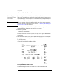
| The ON symbols are
used to mark the positions of the instrument
power line switch.
Exclusive Remedies.
The remedies provided herein
are buyer's sole and exclusive
remedies. Agilent Technologies shall not be liable for any
direct, indirect, special, incidental, or consequential damages, whether based on
contract, tort, or any other
legal theory.
❍ The OFF symbols
are used to mark the
positions of the instrument power line
switch.
Safety Symbols.
CAUTION
The CE mark is a registered trademark of
the European Community.
The caution sign denotes a
hazard. It calls attention to a
procedure which, if not correctly performed or adhered
to, could result in damage to
or destruction of the product.
Do not proceed beyond a caution sign until the indicated
conditions are fully understood and met.
The CSA mark is a registered trademark of
the Canadian Standards Association.
The C-Tick mark is a
registered trademark
of the Australian Spectrum Management
Agency.
WARNING
The warning sign denotes a
hazard. It calls attention to a
procedure which, if not correctly performed or adhered
to, could result in injury or
loss of life. Do not proceed
beyond a warning sign until
the indicated conditions are
fully understood and met.
The instruction manual symbol. The product is marked with this
warning symbol when
it is necessary for the
user to refer to the
instructions in the
manual.
The laser radiation
symbol. This warning
symbol is marked on
products which have a
laser output.
The AC symbol is used
to indicate the
required nature of the
line module input
power.
ISM1-A
This text denotes the
instrument is an
Industrial Scientific
and Medical Group 1
Class A product.
Typographical Conventions.
The following conventions are
used in this book:
Key type for keys or text
located on the keyboard or
instrument.
Softkey type for key names that
are displayed on the instrument’s screen.
Display type for words or
characters displayed on the
computer’s screen or instrument’s display.
User type for words or characters that you type or enter.
Emphasis type for words or
characters that emphasize
some point or that are used as
place holders for text that you
type.
General Safety Considerations
General Safety Considerations
This product has been designed and tested in accordance with the standards
listed on the Manufacturer’s Declaration of Conformity, and has been supplied
in a safe condition. The documentation contains information and warnings
that must be followed by the user to ensure safe operation and to maintain the
product in a safe condition.
Install the instrument according to the enclosure protection provided.
This instrument does not protect against the ingress of water.
This instrument protects against finger access to hazardous parts within the
enclosure.
WARNING
If this product is not used as specified, the protection provided by the
equipment could be impaired. This product must be used in a normal
condition (in which all means for protection are intact) only.
WARNING
No operator serviceable parts inside. Refer servicing to qualified
service personnel. To prevent electrical shock do not remove covers.
WARNING
This is a Safety Class 1 Product (provided with a protective earthing
ground incorporated in the power cord). The mains plug shall only be
inserted in a socket outlet provided with a protective earth contact.
Any interruption of the protective conductor inside or outside of the
instrument is likely to make the instrument dangerous. Intentional
interruption is prohibited.
WARNING
To prevent electrical shock, disconnect the instrument from mains
before cleaning. Use a dry cloth or one slightly dampened with water
to clean the external case parts. Do not attempt to clean internally.
WARNING
For continued protection against fire hazard, replace line fuse only
with same type and ratings (type nA/nV). The use of other fuses or
materials is prohibited.
iii
General Safety Considerations
CAUTION
Fiber-optic connectors are easily damaged when connected to dirty or
damaged cables and accessories. The Agilent 71501D’s front-panel input
connector is no exception. When you use improper cleaning and handling
techniques, you risk expensive instrument repairs, damaged cables, and
compromised measurements. Before you connect any fiber-optic cable to the
Agilent 71501D clean it thoroughly.
CAUTION
This product is designed for use in Installation Category II and Pollution
Degree 2 per IEC 61010-1C and 664 respectively.
CAUTION
Always use the three-prong ac power cord supplied with this instrument.
Failure to ensure adequate earth grounding by not using this cord may cause
instrument damage.
CAUTION
This instrument has autoranging line voltage input. Be sure the supply voltage
is within the specified range.
CAUTION
Use of controls or adjustment or performance of procedures other than those
specified herein may result in hazardous radiation exposure.
iv
Contents
1 Getting Started
Steps for Setting Up Eye-Diagram Analysis 1-4
2 Application Tutorials
Tutorial 1: Measure Eye-Parameters 2-4
Tutorial 2: Measure in Optical Power Units 2-8
Tutorial 3: Measure Extinction Ratios on Low-Level Signals 2-10
Tutorial 4: Measure Laser Turn-on Delay 2-13
Tutorial 5: Use Software Filters 2-15
Tutorial 6: Test to Industry Standards 2-19
Tutorial 7: Default and Custom Mask or
Limit Line Testing 2-23
Tutorial 8: Display the Data Pattern 2-27
Tutorial 9: Constructing a Low-Pass Filter from a Transfer Function 2-30
Tutorial 10: Create a Vertical Histogram 2-36
Tutorial 11: Create a Horizontal Histogram 2-41
3 Eye-Diagram Analyzer Reference
Performing Eye-Diagram Measurements 3-3
Generating Histograms 3-7
Masks and Limit Lines 3-9
Eye-Diagram Menu Maps 3-12
Agilent 70820A Menus 3-14
Controlling the Display 3-16
Calibrating the Eye-Diagram Analyzer 3-23
Displaying Traces 3-25
Using Markers 3-30
Applying Mask Testing 3-31
Saving to Mass Storage 3-34
Creating Copies of the Display 3-47
Agilent 70820A User-Corrections 3-49
Agilent 70820A Calibration 3-61
4 Programming Commands
Introduction 4-3
Contents-1
Contents
5 Specifications and Characteristics
Vertical Specifications 5-3
Input Channel Specifications 5-4
Trigger Specifications 5-5
Trigger Specifications 5-6
Horizontal Specifications 5-7
Declaration of Conformity 5-8
Contents-2
1
Getting Started
Getting Started
Getting Started with the Eye-Diagram Analyzer
Getting Started with the Eye-Diagram
Analyzer
In this chapter, you will find information on the following topics:
•
•
•
•
•
•
Steps for Setting Up Eye-Diagram Analysis 1-4
Step 1. Connect the Equipment 1-12
Step 2. Load the Personality 1-16
Step 3. Complete the Installation Using the Screen Instructions
Step 4. Set Up the Measurement Conditions 1-22
Optional Step. Save Instrument State as Preset State 1-26
1-19
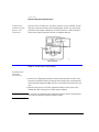
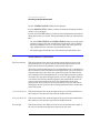
The Agilent 71501D Eye-Diagram Analysis
You can configure the 71501D system as a high-speed eye-diagram analyzer
using Option 005 eye-diagram analysis software. This software allows the system to operate similar to a high-speed sampling oscilloscope such as the Agilent 86100A Infiniium DCA.
The 71501D can perform eye-diagram analysis such as extinction-ratio testing
and mask testing. In addition, the software allows the system to operate in
Agilent Eyeline mode. In eyeline mode the eye-diagram display shows continuous traces instead of synchronous dots. This allows pattern dependent
effects to be investigated. For example, the trace leading to a mask violation
can be captured and displayed. The eyeline eye-diagram can take advantage of
trace averaging. Therefore, very small energy signals can be extracted from
broadband noise. Finally, eye-diagrams can be analyzed using software filters.
Fourth-order Bessel-Thompson filters can be easily designed for virtually any
data rate allowing analysis without having to actually construct a hardware filter.
Getting Started
Getting Started with the Eye-Diagram Analyzer
The custom keypad
The eye-diagram analyzer comes with a custom keypad that snaps into the
front panel of 70004A displays. The keypad gives you quick access to common
instrument functions. (Each of these functions can also be accessed using the
normal softkey menus.)
If you have the custom keypad, practice using it. You will find that the time
required, for many of the procedures in this book, will be significantly
reduced.
CAUTION
If you need to remove the custom keypad, do not pry it out. Simply push the tip
of a small flat-blade screwdriver straight into the removal hole, and the keypad
will pop out.
1-3
Getting Started
Steps for Setting Up Eye-Diagram Analysis
Steps for Setting Up Eye-Diagram Analysis
1 Connect the equipment.
2 Load the eye-diagram personality.
3 Complete the installation using the self-guided screens.
4 Set up the measurement conditions.
Connect the
Equipment
You can connect the equipment in three possible configurations:
• With 70841A/B pattern generator and 70311 clock source modules. This is
the preferred configuration.
• With an 70841 pattern generator module with a non- 70311 clock source
module.
• With non- MMS70841 pattern generator and clock source modules.
Load the EyeDiagram
Personality
Each time the 71501D is turned on, the 70874A eye-diagram analyzer personality (part number 70874-10001) must be loaded into memory. This occurs
automatically if the 70874A memory card is inserted in the front-panel card
slot before the instrument is turned on. You can also load the personality in a
manual mode.
Complete the
Installation Using
Self-Guided
Screens
Installing the eye-diagram analyzer is easy due to a series of self-guided
screens. Depending on the factory configuration of your system, one or more
of these screens may not be displayed.
After connecting the equipment and loading the program, you’ll need to
respond to a series of screens from which to select the following:
• The pattern generator used.
• The source of the 10 MHz frequency reference.
Getting Started
Steps for Setting Up Eye-Diagram Analysis
Note
When used with an 71612A/70843, the system requires a manual configuration.
Set Up the
Measurement
Conditions
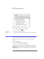
Select from eye, eyeline, and pattern modes
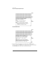
Use the Setup menu’s diagram softkey to select from one of three measurement modes: eye, eyeline, and pattern.
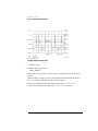
Features Available in Each Mode
Eye Mode
Eyeline Mode
Eye Measurements
X
Extinction Ratio Measurements
X
X
Mask Testing
X
Pattern Mode
X
X
Display the Mask Error Trace
X
X
Improve Sensitivity Using Eye Filtering
X
X
40 GHz Extended Bandwidth
X
X
User-Corrections
X
Display Data Pattern
X
X
1-5
Getting Started
Steps for Setting Up Eye-Diagram Analysis
Eye Mode
The eye mode displays traces using individual dots in a manner that is similar
to conventional sampling oscilloscopes. Use this mode for the following:
• Typical eye-diagram measurements
• Extinction ratio measurements
Getting Started
Steps for Setting Up Eye-Diagram Analysis
Eyeline Mode
: Eyeline mode displays continuous traces. Use this mode for the following:
•
•
•
•
•
•
Measure extinction ratio
Measure laser turn-on transition delay
Examine laser overshoot
Observe laser ringing
Apply eye-filter
Apply user-corrections
1-7
Getting Started
Steps for Setting Up Eye-Diagram Analysis
Pattern Mode
Pattern mode displays the actual PRBS data stream bits. This mode uses the
pattern trigger which allows the display to show the same portion of the data
stream from sweep to sweep.
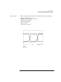
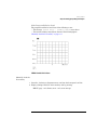
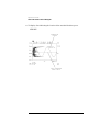
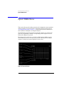
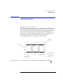
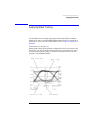
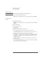
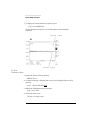
Mask/limit lines provide pass/fail testing
Mask/limit lines are displayed geometric shapes that define the acceptable
limits and shape of an eye-diagram. The following figure shows a mask. Use
masks for pass/fail testing and as an aid to error analysis. The eye-diagram
analyzer can capture and display the portion of the pattern that caused a mask
violation. Built-in standard masks for the major SONET/SDH transmission
rates are provided and can be applied with the press of a softkey. Or, you can
create your own custom masks.
Getting Started
Steps for Setting Up Eye-Diagram Analysis
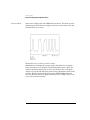
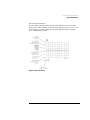
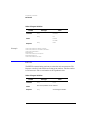
Apply software filters in eyeline mode
In eyeline mode, user frequency corrections can be applied to the data to simulate a hardware transmission filter. The eye-diagram analyzer comes with
several Bessel-Thomson filters. These files are on the 71501D memory card.
Refer toChapter 9, “Agilent 70820A: User Corrections” and Chapter 11, “Agilent 70820A: Memory Cards, Disks, and RAM”for information on user-corrections.
User Correction Files
File Name
File Data
a_bt248832
4th order Bessel-Thomson filter for 2.48832 Gbit/sec transmission
a_bt_62208
4th order Bessel- Thomson filter for 622.08 Mbit/sec transmission
a_bt_15552
4th order Bessel- Thomson filter for 155.52 Mbit/sec transmission
1-9
Getting Started
Steps for Setting Up Eye-Diagram Analysis
Three sweep selections are available
• single
• continuous
• stopped
With the continuous selection, sweeps occur as soon as the selected triggering
conditions are met and repeat continuously as long as the trigger conditions
are met.
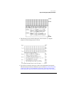
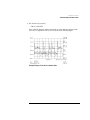
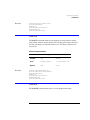
The source of the trigger reference is selected using the Setup menu’s CH2
softkey. The following table shows the reference used when using an Agilent
7084X pattern generator.
Table 1-1.
Trigger Reference of 70841
Eye Mode
CLOCKa or TRIGGER
CLOCK or TRIGGER
TRIGGER
a. This connection provides faster trace updates.
Entering the pattern generator’s settings
The Setup menu’s READ PAT GEN softkey queries the 70841 pattern generator and 70311A signal generator for the clock frequency, pattern length, and
any divide ratios. In the case of alternate configurations, an appropriate submenu will be displayed for the parameters that require manual updating.
Note
A READ PAT GEN should be performed after changing pattern generator
settings, such as clock frequency or pattern length.
Moving the measurement plane
Specifying an attenuation on channel 1 changes the measurement plane from
the front-panel RF INPUT 1 connector to include the indicated attenuation.
Specifying any attenuation on channel 2 may be necessary to ensure proper
triggering. Use the Trg,Cal menu’s CH1 EXT ATTEN and CH2 EXT ATTEN
softkeys to specify any external attenuation.
Getting Started
Steps for Setting Up Eye-Diagram Analysis
These softkeys can also be used to specify an optical-to-electrical responsivity
conversion between the source and input channels. As a result, the display
shows optical units referenced to the input of the optical-to-electrical converter. Channel and marker readouts change to watts/div. Also, the CH1 EXT
ATTEN softkey changes to read CH1 RSPVTY (responsivity).
Autoranging
The Trg,Cal menu’s autorng ON OFF softkey turns on or off autoranging.
When autoranging is activated, the eye-diagram analyzer automatically selects
the appropriate hardware gain and offset to maximize the signal at the analogto-digital converter, regardless of the input signal’s amplitude.
Selecting the 10 MHz reference on Instrument Preset
Use the Trg,Cal menu’s IP REF softkey to select the source of the 10 MHz reference on an INSTR PRESET. Choices are internal, external, or auto. With
auto, the eye-diagram automatically selects an external reference if it is
present at the 70820A’s rear-panel connector. Otherwise, the module’s internal reference is selected.
Redefining the INSTR PRESET key
The Trg,Cal menu’s DEFINE USER IP softkey redefines the settings invoked
by the INSTR PRESET key. Redefining the instrument preset can save valuable time when configuring for measurements.
1-11
Getting Started
Steps for Setting Up Eye-Diagram Analysis
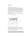
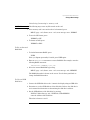
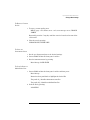
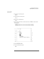
Step 1. Connect the Equipment
70841A/B Pattern
Generator and
70311A Signal
Generator
Modules
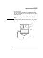
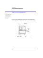
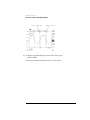
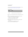
1 If you are using 70841A/B pattern generator and 70311A signal generator
modules with your eye-diagram analyzer, install them into an MMS mainframe
as shown in the following figure.
Getting Started
Steps for Setting Up Eye-Diagram Analysis
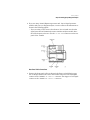
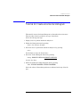
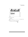
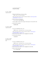
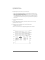
2 If you are using 70841A/B pattern generator and 70311A signal generator
modules with your eye-diagram analyzer, connect cables to the instruments as
shown in the following graphic.
• If you are using a clock source other than an 70311A, make sure that the
signal generator and 70820A microwave transition analyzer module share
the same frequency reference. Use the 10 MHz REF connectors on the rear
panel of the 70820A.
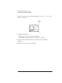
Rear-Panel Cable Connections
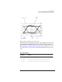
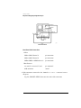
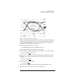
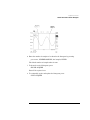
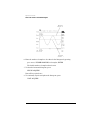
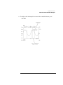
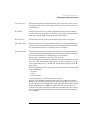
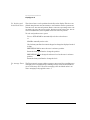
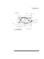
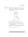
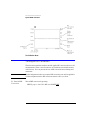
3 Connect the front-panel cables as shown in the figure on the following page.
Use an adapter between the cables and channel connectors. The data signal
connects to the 70820A’s RF INPUT 1 connector. The trigger or clock signal
connects to the 70820A’s RF INPUT 2 connector.
1-13
Getting Started
Steps for Setting Up Eye-Diagram Analysis
Front-Panel Cable Connections
Cables:
SMA to SMA (Channel 1)
p/n 8120-4948
SMA to SMA (Channel 2)
p/n 8120-4948
SMB to SMB (10 MHz Reference)
p/n 8120-5025
Miscellaneous:
3.5 mm (f) to 2.4 mm (f) (two)
p/n 1250-2277
6 dB attenuator
8493C
4 If the attenuator connected to the 70820A’s RF INPUT 2 connector is not 6
dB, press:
Trg,Cal, CH2 EXT ATTEN, then enter the value of the attenuator
Getting Started
Steps for Setting Up Eye-Diagram Analysis
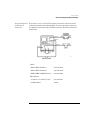
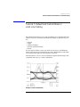
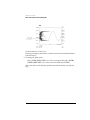
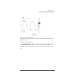
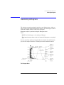
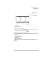
Laser and Optical- If you have access to a laser and an optical-to-electrical converter, use the
to-Electrical
connections shown in the following figure. To protect the input connectors,
Converter
use adapters between the cables and the connectors. The laser is the device
being tested.
Cables:
SMA to SMA (Channel 1)
p/n 8120-4948
SMA to SMA (Channel 2)
p/n 8120-4948
SMB to SMB (10 MHz Reference)
p/n 8120-5025
Miscellaneous:
3.5 mm (f) to 2.4 mm (f) (two)
p/n 1250-2277
6 dB attenuator
8493C
1-15
Getting Started
Steps for Setting Up Eye-Diagram Analysis
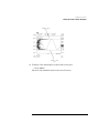
Connections
without a Laser
Source and
Converter
If a laser source and optical-to-electrical converter are not available, use the
alternate connection shown in the following figure. In this case, the pattern
generator’s data output is displayed. An electrical device could be inserted
between the pattern generator and the eye-diagram analyzer.
Step 2. Load the Personality
Automatically
Load the
Personality
1 Insert the eye-diagram personality card into the front-panel card slot of the
microwave transition analyzer, facing the metal strip on the card downward
and toward the instrument. Make sure the card is fully inserted into the card
slot.
2 Switch on the power to all of the equipment. Switch on the power to the
70820A last. The start up process takes about 6 minutes.
Note
Do not press any instrument keys until the program is loaded. Pressing keys
can cause the automatic program loading to abort.
Getting Started
Steps for Setting Up Eye-Diagram Analysis
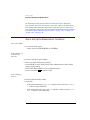
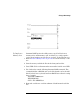
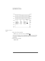
If the Program Failed to Load
The program has failed to load if one of the following occurs:
• The message Please wait... Loading 70874 never shows.
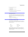
• The left-side softkeys match those shown in the following figure.
“Manually Load the Personality” on page 1-17
70820A Module’s Main Menu
Manually Load the
Personality
1 Insert the 70874A eye-diagram memory card into the front-panel card slot.
2 Display a listing of the files on the memory card by pressing:
MENU, page 1 of 2, States, more 1 of 2, mass storage
1-17
Getting Started
Steps for Setting Up Eye-Diagram Analysis
3 If the screen does not resemble the above figure, press:
msi:, HP-MSIB CARD, prev menu
DISPLAY, Mass Storage, msi, MEMORY CARD
MENU
The list of files should now be displayed.
4 Turn the front-panel knob to highlight the file "AUTOST" and then press:
LOAD FILE
If you load the "70874" file by mistake, the message 7386 memory overflow may be displayed. This error message is a result of the manual loading process and, in this instance, does not indicate a problem. The program still should be
properly loaded.
Getting Started
Steps for Setting Up Eye-Diagram Analysis
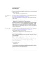
Step 3. Complete the Installation Using the
Screen Instructions
• If the displayed screen looks like the figure on the left side of this page, your
system has been previously configured. Press CONT and then continue with
"Step 4. Connect the front-panel cables". However, if you wish to reconfigure
your system, press RECNFIG, and continue with the following explanation of
the self-guided screens.
• If the screen looks like the figure on the right side of this page, the first selfguided screen is displayed. Perform the following steps:
1 Press 7084X if you are using an 70841A/B pattern generator. If using an
70843A, or any other pattern generator, press MANUAL.
2 If you press 7084X, the screen shown on the following page is displayed. The
program automatically determines and displays the pattern generator module’s
HP-MSIB address. For most installations, press CONT. To manually enter the
HP-MSIB address, use the displayed softkeys.
Example of a Configuration Previously Done
1-19
Getting Started
Steps for Setting Up Eye-Diagram Analysis
First Self-Guided Screen
3 Use the following self-guided screen to indicate the 10 MHz frequency
reference used. Press INTERNL if the 70820A module is used as the reference.
Press EXTERNL if the clock source is used as the reference.
Getting Started
Steps for Setting Up Eye-Diagram Analysis
4 The following screen should be displayed. Notice that the eye-diagram
analyzer’s left-side Setup menu is selected.
5 If you have not already connect the cables to the instruments’ front panels,
follow the instructions shown. Otherwise, proceed with “If you have not already
connect the cables to the instruments’ front panels, follow the instructions
shown. Otherwise, proceed with “If you have not already connect the cables to
1-21
Getting Started
Steps for Setting Up Eye-Diagram Analysis
the instruments’ front panels, follow the instructions shown. Otherwise,
proceed with “If you have not already connect the cables to the instruments’
front panels, follow the instructions shown. Otherwise, proceed with “If you
have not already connect the cables to the instruments’ front panels, follow the
instructions shown. Otherwise, proceed with .” on page 1-21.” on page 1-21.”
on page 1-22.” on page 1-22.
Step 4. Set Up the Measurement Conditions
Select the Mode
1 To select the mode, press:
Setup, diagram, EYE, EYELINE, or PATTERN
Select Single or
Continuous
Sweeps
2 Press the left-side Trg,Cal softkey.
3 Select one of the following sweep states:
• Press SINGLE to select single sweeps. Each additional press of this softkey
triggers another sweep.
• Press CONT STOP CONT to select continuous sweeps.
• Press CONT STOP STOP to stop the sweeps.
Select Trigger
Source
4 Press the left-side Setup softkey.
5 Press CH2.
• If the pattern generator’s CLOCK OUT signal is connected to the RF INPUT
2 connector, press CLK OUT.
• If the pattern generator’s TRIGGER OUT signal is connected to the RF INPUT 2 connector, press TRG OUT.
Getting Started
Steps for Setting Up Eye-Diagram Analysis
Note
Using the CLOCK OUT trigger signal provides faster data acquisition for eyediagrams. If the amplitude of the trigger signal is too large, an over-range
message is displayed. If a message is displayed, reduce the amplitude of the
signal; use an external attenuator, and enter the value using CH2 EXT ATTEN.
Select the Pattern
Generator
Settings
6 If an 70841A/B pattern generator is used, press READ PAT GEN.
7 The eye-diagram analyzer reads the settings of the pattern generator.
8 If a pattern generator, such as the 70843A/71612A, is used in place of an
70841A/B pattern generator, press:
READ PAT GEN, CLOCK RATE and enter the rate of the clock signal
CLOCK DIVISOR and enter the divisor for the clock signal
For example, when using a trigger or sync output, enter 16 if the clock signal
is divided by 16.
9 Enter the pattern repetition length by pressing:
PATTERN LENGTH and enter the pattern repetition length
The pattern repetition length is entered in bits or as the binary power depending on the position of the 2^n-1 ON OFF softkey. If the function is on, binary
powers are entered in the form 2n–1. This makes it very easy to set the pattern
length for PRBS sequences. When the function is off, the pattern length is
entered directly in bits.
10 Press PAT TRG FACTOR, and enter the factor that relates how many
repetitions of the pattern occur between trigger pulses.
Frequently, 16 to 32 or more repetitions of the pattern occur between trigger
pulses.
Note
When operating off a trigger or sync output with a divided clock frequency or
a pattern trigger, be sure to set CH2 is: to TRG OUT.
11 If a signal generator other than the 70311A is used, enter the precise clock
frequency by pressing:
prev menu, CLOCK RATE and enter the clock rate
1-23
Getting Started
Steps for Setting Up Eye-Diagram Analysis
Controlling an
70841A/B Pattern
Generator
When using the 70311A clock source (below 3 Gb/s):
This section explains how to display the menus for the 70841A/B pattern generator. The display can be assigned to control either the eye-diagram analyzer
or the 70841A/B pattern generator.
Note
If the eye-diagram analyzer is configured with a non 70841 pattern generator,
you must manually set the trigger level. Refer to “To Manually Set the Trigger
Level” on page 1-25 in this chapter.
1 Turn on the power for both mainframes. Wait until the start-up routines are
completed and the mainframes are ready for key presses.
2 Continue by pressing:
DISPLAY, NEXT INSTR
If several instruments are in the system, you may have to press NEXT INSTR
several times.
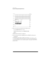
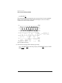
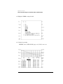
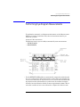
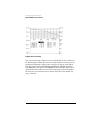
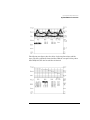
3 If the 70841A/B’s status screen, shown in the following figure, is not shown, the
pattern generator is probably addressed as a slave instead of a master. Perform
the following steps:
a Press the left-side Address Map softkey.
An Example 70841A/B’s Status Screen
b Use the front-panel knob to scroll the box to the column where the
Getting Started
Steps for Setting Up Eye-Diagram Analysis
70841A/B appears.
c Press ADJUST ROW, and rotate the knob to move the box to the row where
the 70841A/B appears.
d Press ASSIGN BOTH.
4 Use the displayed softkey menus to set the pattern generator to the desired
settings. For an example, refer to the paragraph "Configure the data signal" in
Chapter 2, “Application Tutorials”.
5 To return control to the eye-diagram analyzer, press:
DISPLAY, NEXT INSTR
6 To return to the eye-diagram analyzer personality menus, press:
USER
To Manually Set
the Trigger Level
If a pattern generator other than the 70841A/B is used, you must use the following procedure to manually set the trigger level.
1 Select trace two and turn the display on by pressing:
> prev menu, select:, TR2, display ON/OFF ON
2 Automatically scale the trigger trace and set the trigger level by pressing:
AUTO-SCALE, Trg,Cal, LEVEL
Use the knob to position the trigger level indicator line so it crosses an edge.
1-25
Getting Started
Steps for Setting Up Eye-Diagram Analysis
3 Turn the display off and select trace one by pressing:
Traces, display ON|OFF OFF, select:, TR1
Move the
Measurement
Plane
To move the measurement plane, press:
Trg,Cal, CH1 EXT ATTEN and enter the attenuation on channel 1 input.
Optional Step. Save Instrument State as Preset State
1 Select the Traces menu and scale the screen to the displayed signal by
pressing:
Traces, AUTOSCALE
2 Save the current instrument state by pressing:
Trg,Cal, more 1 of 2, DEFINE USER IP, CONT
The current instrument state is saved, including the pattern generator’s HPMSIB address, the frequency reference, scaling, and trigger level. Whenever
INSTR PRESET is pressed, the eye-diagram analyzer is automatically placed
in these settings.
Getting Started
Steps for Setting Up Eye-Diagram Analysis
3 The eye-diagram is now ready for use.
To restore the
Restore the factory instrument preset by pressing:
factory
MENU, page 1 of 2, States, more 1 of 2, preset: FAC|USR FAC
instrument preset
1-27
Getting Started
Steps for Setting Up Eye-Diagram Analysis
2
Application Tutorials
Application Tutorials
Application Tutorials
Application Tutorials
This chapter contains nine tutorials that introduce important eye-diagram
analyzer features. The tutorials should be performed in the order listed. To
create the data signal, you will need a pseudo-random binary sequence
(PRBS) pattern generator. Refer to “Configure the Data Signal” on page 2-2
before you start the tutorials. You will find the following topics in this chapter:
•
•
•
•
•
•
•
•
•
•
•
Tutorial 1: Measure Eye-Parameters 2-4
Tutorial 2: Measure in Optical Power Units 2-8
Tutorial 3: Measure Extinction Ratios on Low-Level Signals 2-10
Tutorial 4: Measure Laser Turn-on Delay 2-13
Tutorial 5: Use Software Filters 2-15
Tutorial 6: Test to Industry Standards 2-19
Tutorial 7: Default and Custom Mask or Limit Line Testing 2-23
Tutorial 8: Display the Data Pattern 2-27
Tutorial 9: Constructing a Low-Pass Filter from a Transfer Function
Tutorial 10: Create a Vertical Histogram 2-36
Tutorial 11: Create a Horizontal Histogram 2-41
2-30
Configure the Data Signal
The following list shows typical settings that can be used for the data signal.
The list assumes you are using an 70841A/B pattern generator. The exact settings depend upon the system you are using. If the system includes an
70841A/B pattern generator, use the pattern generator’s status screen to enter
these values. The procedure for viewing the status screen is explained in
“Controlling an 70841A/B Pattern Generator” on page 1-24.
• In the select pattern menu:
Pattern: PRBS 2^7-1
• In the dat o/p err-add menu:
Data Ampl: typically 800 mV to 2 V (depending on laser)
Data Hi-Lvl: 0 V (depending on laser)
• In the trg o/p clk o/p menu:
Application Tutorials
Application Tutorials
Clock Freq: 2.48832 GHz
Clock Ampl: 500 mV
Clock Hi-Lvl: 0 V
If you’re performing these tutorials without the laser source and optical-toelectrical converter, reduce the level of the data signal as shown in the following settings:
• Data Ampl 250 mV
• Data Hi-Lvl 300 mV
2-3
Application Tutorials
Tutorial 1: Measure Eye-Parameters
Tutorial 1: Measure Eye-Parameters
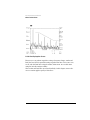
The eye-diagram analyzer performs automatic eye measurements in eye
mode. This mode is similar to that of conventional sampling oscilloscopes; the
display shows individual dots.
View the Signal
1 To view the signal, press:
INSTR PRESET, Traces, persist, VARIABL
This turns the persistence mode on. Refer to Chapter 3, “Eye-Diagram Analyzer Reference” for an explanation of the available persistence modes.
2 Enter the number of sweeps by pressing:
PERSIST SWEEPS and enter 8
3 Turn autoscaling on by pressing:
prev menu, AUTO-SCALE
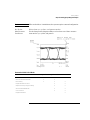
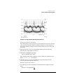
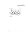
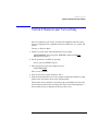
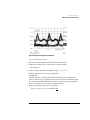
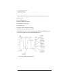
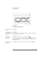
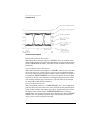
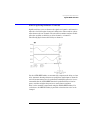
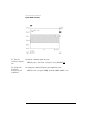
The display should look similar to the display of a sampling oscilloscope. See
the following figure.
The large overshoot shown is a result of the particular laser bias setting used.
If the edges of the waveform are unstable in time (indicating no trigger), refer
to the “To Manually Set the Trigger Level” on page 1-25.
Application Tutorials
Tutorial 1: Measure Eye-Parameters
Example of a Large Overshoot Resulting from Laser Bias
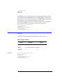
Perform an Offset Calibration
This calibration procedure removes any offset that may be present in the optical-to-electrical converter. This is sometimes referred to as the "dark" level.
The offset calibration ensures accurate measurements of the laser’s one and
zero levels.
4 Turn the laser off. (If you are measuring the pattern generator directly,
disconnect the input signal at channel 1.)
5 Perform the calibration by pressing:
Trg,Cal, OFFSET CAL, CONT
The calibration takes about a minute to execute. When the calibration is finished, DC NULL: done is displayed.
6 Turn the laser on. (If you are measuring the pattern generator directly,
reconnect the input signal at channel 1.)
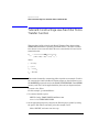
Measure Signal Parameters
7 To include the rise time and fall time measurement in the displayed results,
press:
Measure, r/f tim ON OFF ON
2-5
Application Tutorials
Tutorial 1: Measure Eye-Parameters
Enabling this function approximately doubles the measurement time.
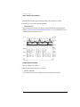
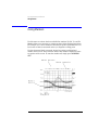
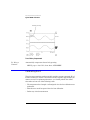
8 Perform the eye measurement by pressing:
MEASURE EYE
After a brief period of time, the display should look like the following figure.
Refer to Chapter 3, “Eye-Diagram Analyzer Reference” for definitions of each
measurement listed on the screen.
Example Eye Measurements
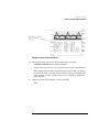
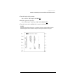
Measure Extinction Ratio
9 Measure the extinction ratio by pressing:
EXTINCT RATIO
The results are added to the displayed list of measurement results.
Application Tutorials
Tutorial 1: Measure Eye-Parameters
Example Extinction Ratio Measurement
10 Change the amount of data used for the histograms by pressing:
NUMBER SAMPLES and enter the # of samples
A larger value gives more accuracy, but increases the data acquisition time.
When making extinction ratio measurements in eyeline mode, the number
of samples should be increased from the default of 1000 to something on the
order of 20000 to insure a number of traces are evaluated to compute the
extinction ratio.
11 Clear the measured data from the screen by pressing:
OFF
2-7
Application Tutorials
Tutorial 2: Measure in Optical Power Units
Tutorial 2: Measure in Optical Power Units
The analyzer display has the ability to show optical units referenced to the
input of the optical-to-electrical converter. This changes the channel and
marker readouts to watts/div.
1 Set the analyzer to a known state by pressing:
INSTR PRESET, Trg,Cal, CH1 EXT ATTEN responsivity value,
V/Watt
For example, the following figure shows 350 V/Watt entered. Notice the softkey label changes to CH1 RSPVTY (responsivity).
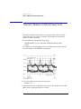
2 To use the markers to read optical power, press:
Markers, Y1 (--)
3 Adjust the marker line to the peak of the response. For example, the following
figure shows a peak optical power of 1.5 mW.
Application Tutorials
Tutorial 2: Measure in Optical Power Units
2-9
Application Tutorials
Tutorial 3: Measure Extinction Ratios on Low-Level Signals
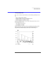
Tutorial 3: Measure Extinction Ratios on LowLevel Signals
Repeatable extinction ratio measurements can be made on low-level signals.
This is accomplished by applying a filter to the signal. This filter improves
measurement sensitivity and is useful for analyzing:
• low-level extinction ratios
• pattern dependent transitions
• intersymbol interference
In this tutorial, the eye-diagram analyzer is placed in eyeline mode so that the
eye filter can be applied to reduce trace noise. To measure the signal, a photodiode converter with a responsivity of 30 volts/watt is used.
When making extinction ratio measurements in eyeline mode, the number of
samples should be increased from the default of 1000 to something on the
order of 20000. This insures a number of traces are evaluated to compute the
extinction ratio. The compatible mode is eyeline.
Change to Eyeline Mode
1 Set the instrument to a known state by pressing:
INSTR PRESET, Setup, diagram, EYELINE, Traces
2 Set the number of persistence sweeps by pressing:
persist, VARIABL, PERSIST SWEEPS and enter 5, prev menu
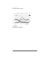
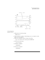
3 Turn on autoscaling by pressing:
Trg,Cal, more 1 of 2, Traces, AUTO-SCALE
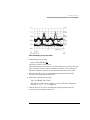
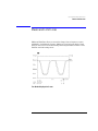
The display should look like the following figure.
A low-amplitude response, similar to that shown in this figure, can result when
using non-amplified lightwave converters to measure optical signals.
Application Tutorials
Tutorial 3: Measure Extinction Ratios on Low-Level Signals
Autoscaled Display of Low-Level Signal
4 Turn filtering on by pressing:
Setup, eyefltr ON OFF ON
Perform an Offset Calibration
This calibration procedure removes any offset that may be present in the optical-to-electrical converter. This is sometimes referred to as the "dark" level.
The offset calibration ensures accurate measurements of the laser’s level.
5 Turn the laser off. (If you are measuring the pattern generator directly,
disconnect the input signal at channel 1.)
6 Perform the calibration by pressing:
Trg,Cal, OFFSET CAL, CONT
The calibration takes about a minute to execute. When the calibration is
finished, DC NULL: done is displayed.
7 Turn the laser on. (If you are measuring the pattern generator directly,
reconnect the input signal at channel 1.)
2-11
Application Tutorials
Tutorial 3: Measure Extinction Ratios on Low-Level Signals
Measure the Extinction Ratio
8 To measure the extinction ratio, press:
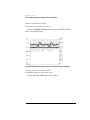
Measure, NUMBER SAMPLES and enter 20000, EXTINCT RATIO
Refer to the following figure.
Extinction Ratio Measurement on a Low-Level Signal with Eye Filtering On
Display the Signal in Optical Units
9 To display the signal in optical units, press:
Trg,Cal, CH1 EXT ATTEN and enter 30 V/Watt
Application Tutorials
Tutorial 4: Measure Laser Turn-on Delay
Tutorial 4: Measure Laser Turn-on Delay
On-screen markers can be used to measure both amplitude and time separation in eye-diagrams. The compatible modes for markers are eye, eyeline, and
pattern.
Change to Eyeline Mode
1 Change to eyeline mode, then turn filtering on by pressing:
INSTR PRESET, Setup, diagram, EYELINE, eyefltr ON OFF ON,
BIT INTVL and enter 1
2 Set the persistence to infinite by pressing:
Traces, persist, INFINIT, Trg,Cal
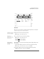
3 After several traces have been displayed, press:
CONT STOP STOP
Turn on the markers
4 Press X1 and X2 to activate markers 1 and 2.
5 Turn the front-panel knob to move the markers to different transition crossing
points on the waveform as show in the following figure.
This provides an easy method to check the peak-to-peak difference in the laser
turn-on time measured at the crossing point. Notice in the following figure, a
delta reading of 30 ps is displayed at the top of the screen.
2-13
Application Tutorials
Tutorial 4: Measure Laser Turn-on Delay
Laser Overshoot and Turn-On Delay
Application Tutorials
Tutorial 5: Use Software Filters
Tutorial 5: Use Software Filters
This tutorial enables a software filter. The filter is designed with user frequency corrections. User frequency corrections can be used for:
• Removing the effects of frequency response roll-off due to the optical-toelectrical converter and cables.
• Simulating hardware filters recommended for laser transmitter evaluation,
such as 4th-order Bessel- Thomson filters.
The eye-diagram analyzer must be in eyeline mode to apply user-corrections.
In eyeline mode, each sweep produces a continuous trace with the points connected. (This is opposed to unconnected dots with the eye mode.) Eyeline
mode is especially useful for measuring variations in laser turn-on delay, overshoot, and ringing and for applying user frequency corrections. The compatible mode is eyeline.
Several Bessel-Thomson software filters are included on the 70874A eye-diagram analyzer’s memory card. These filters can be applied as user-corrections
in the eyeline and pattern modes. (User corrections must be off in eye mode.)
User correction files are identified by the prefix a_ as shown in the following
table. Two additional files on the card, AUTOST and 70874, comprise the eyediagram analyzer program.
Supplied User-Correction Files
File Name
File Data
a_bt248832
4th order Bessel- Thomson filter for 2.48832 Gbit/sec transmission.
a_bt_62208
4th order Bessel- Thomson filter for 622.08 Mbit/sec transmission.
a_bt_15552
4th order Bessel- Thomson filter for 155.52 Mbit/sec transmission.
2-15
Application Tutorials
Tutorial 5: Use Software Filters
User-Corrections Applied to the Data
Change to Eyeline Mode
1 Set the analyzer to a known state by pressing:
INSTR PRESET, Traces, persist, VARIABL and enter 5, diagram,
EYELINE
Notice the level of the laser overshoot, and the turn-on delay, varies from
sweep to sweep, dependent on the previous pattern of ones and zeros.
Application Tutorials
Tutorial 5: Use Software Filters
Eyeline Display Showing Laser Overshoot
Load the Software Filter
2 Place the 70874A memory card in the front-panel card slot.
3 Display the catalog of files on the memory card by pressing:
Mass Storage
4 Turn the front-panel knob to highlight the file "a_bt248832".
5 Load the file into user-corrections by pressing:
LOAD FILE
This file simulates a 4th-order Bessel-Thomson filter with a cutoff at threequarters of the bit rate. This allows you to observe the laser transmitter signal
in a specified bandwidth. This software filter is equivalent to using a hardware
filter, except that trace noise may be suppressed more.
6 Apply the filter data to the traces by pressing:
Trg,Cal, more 1 of 2, usr cor ON OFF ON
2-17
Application Tutorials
Tutorial 5: Use Software Filters
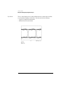
7 Turn the autoscale function on by pressing:
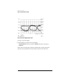
Traces, AUTO-SCALE
The display should look like the following figure.
Notice that the laser overshoot is no longer visible, due to the filtering effect of
the user-corrections in the 71501A.
Example Filtered Laser Overshoot
Application Tutorials
Tutorial 6: Test to Industry Standards
Tutorial 6: Test to Industry Standards
Masks allow you to test eye-diagrams against industry standards. The eye-diagram analyzer provides built-in masks for testing the major SONET/SDH
transmission rates. Compatible modes are eye and eyeline. Shown in this tutorial is the ability to:
• Count mask errors
• Allow for specified amount of margin testing
• Stop after a specified number of trace errors
• Show the violation trace (eyeline mode only)
Select the Mask
1 Set the analyzer to a known state by pressing:
INSTR PRESET
2 You can use your own hardware filter during this tutorial, or load a software
filter as described in the previous tutorial.
3 Set the bit interval and delay by pressing:
Setup, BIT INTVL and enter 1.5, DELAY
Adjust the delay to center the eye.
4 Select a mask by pressing:
Masks, mask setup, default masks, STM-16 OC-48
The display shows an unscaled rectangle mask.
5 Align the mask by pressing:
MASK ALIGN
Wait for the displayed # samp count to reach 100%.
This step aligns the mask to the data using automatic scaling. Notice that, for
the purposes of clarity, the graticule is turned off. This was done using the
70820A Config menu.
2-19
Application Tutorials
Tutorial 6: Test to Industry Standards
Turn Mask Testing On
6 Turn mask testing on by pressing:
Masks, test ON OFF ON
This resets the error counters. Errors for the standard specifications show up
beside the M1 screen annotation for mask violations, and beside L2 and L3 for
upper and lower limit violations, respectively.
Notice that in this case, violations are occurring due to too much overshoot.
Test with Additional Margin
7 Set a 15% mask margin and turn margin testing on by pressing:
mask setup, MASK MARGIN and enter 15, msk mar ON OFF ON
This displays a second set of mask and limit lines for the 15 percent margin.
Errors for the specifications with the specified amount of margin show up
beside the M4, L5 and L6 screen annotations.
The eye-diagram analyzer can count dot (trace point) errors instead of trace
errors. Use the count TRC DOT softkey to make the selection. If a given error
puts 12 trace points within the mask, then the error counter increments by 12.
This is useful for determining the extent of any given error. These features can
be used with either eye or eyeline modes.
Application Tutorials
Tutorial 6: Test to Industry Standards
Stop on and Display Trace Errors
The eye-diagram analyzer has the ability to stop data acquisition when a mask
violation occurs. The number of traces or errors that stop this data acquisition
can be specified. In addition, if you are in eyeline mode, you can separately
display the traces that have caused an error.
8 Set the bit interval and delay by pressing:
Setup, BIT INTVL and enter 1, DELAY and enter –3
The mask will be offset to the right side of the display.
9 Set the analyzer so testing will stop after two errors have occurred by pressing:
#Errors ON OFF ON and enter 2
10 If #Traces is set to on, the eye-diagram analyzer stops sweeping when either
the error or trace limit is reached. Turn the number of traces function off by
pressing:
#Traces ON OFF OFF
11 Turn error tracing on by pressing:
err trc ON OFF ON
Any trace which violates the mask shows on the lower-half of the screen.
12 Reset and start the trace and error counters by pressing:
2-21
Application Tutorials
Tutorial 6: Test to Industry Standards
test ON OFF ON
The instrument stops sweeping after two error traces have been accumulated.
Refer to the following figure. Note that for this figure, errors occur due to
overshoot on a zero-to-one transition.
Turn off Mask Testing
13 Turn off error tracing and the display by pressing:
err trc ON OFF OFF, mask setup, display ON OFF OFF, Trg,Cal, CONT
STOP CONT
Application Tutorials
Tutorial 7: Default and Custom Mask or Limit Line Testing
Tutorial 7: Default and Custom Mask or
Limit Line Testing
The 70820A menus allow you to create and display up to eight limit lines and
masks at one time. Five default mask/limit-line shapes are provided for your
use:
• hexagon
• square
• equilateral triangle
• inverted equilateral triangle
• flat line
You can stretch, shrink, or move any mask. It is also easy to add additional
points or delete unneeded points from any shape. Both limit lines and masks
can establish either upper or lower limits for a response.
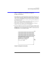
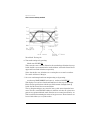
Custom masks are easy to create by editing the supplied default shapes. The
compatible modes are eye, eyeline, and pattern.
Example of a User-Created Mask
2-23
Application Tutorials
Tutorial 7: Default and Custom Mask or Limit Line Testing
Create a Mask or Limit Line
1 Set the analyzer to a known state by pressing:
INSTR PRESET, Setup, BIT INTVL and enter 1.5, Traces, persist,
VARIABL, PERSIST SWEEPS and enter 8
MENU, page 1 of 2, Analyze, masks, limits, define shapes, type:
• If you want to create a mask, press MASK.
• If you want to create a limit line, press UPPER LIMIT or LOWER LIMIT.
Select a Default Mask Shape
2 Select the shape that most closely matches the mask you need. For example,
to display a hexagon, press:
default shapes, hexagon
Edit the Shape
3 To edit the shape, press:
edit
Move a Point
4 To move a point, select the point to be moved by pressing: ⇑ or ⇓
5 Select the direction to move by pressing: move X|Y
Move the point by rotating the front-panel knob or using the numeric keypad.
Add a Point
6 To add a point, select the point to be moved by pressing: ⇑ or ⇓
Note
Select the closest point counterclockwise from the one that you intend to add.
7 Add a point at the location of the currently selected point by pressing: ADD
POINT
A point is inserted between the currently selected point and the next point.
8 Select the direction for moving the new point by pressing: move X|Y
Rotate the front-panel knob to move the point.
Delete a Point
9 To delete a point, select the point to be moved by pressing: ⇑ or ⇓
10 Delete the point by pressing: DELETE POINT
Application Tutorials
Tutorial 7: Default and Custom Mask or Limit Line Testing
Stretch, Reduce, or Move the Mask
11 To stretch, reduce or move the mask by press:
prev menu, scale X|Y or offset X|Y
Add a Mask Margin
12 Press the left-side Masks softkey.
13 To automatically align the mask to a displayed signal, press:
MASK ALIGN
14 To add mask margins, press:
MASK MARGIN and enter the % of needed margin
msk mar ON|OFF ON, prev menu
Begin a Test
15 Display the Masks/Limits menu by pressing:
MENU, page 1 of 2, Analyze, masks, limits
16 Select the trace for testing by pressing:
trace:
17 If trace violations are to be counted as errors, press:
count TRC|DOT TRC
18 If measurement point violations are to be counted as errors, press:
count TRC|DOT DOT
19 To select when testing should stop, press:
end on:
20 If you want testing to stop after a set number of errors, press:
#errors ON|OFF ON desired number of errors
21 If you want testing to stop after a set number of traces, press:
#traces ON|OFF ON desired number of traces
22 To begin testing, press:
test ON|OFF ON
2-25
Application Tutorials
Tutorial 7: Default and Custom Mask or Limit Line Testing
Display the Error Trace
23 Display a mask and begin testing as described in this section, and then press:
err trc ON|OFF ON
Erase a Mask or Limit Line
24 Select the mask or limit line you wish to erase by pressing:
MENU, page 1 of 2, Analyze, masks, limits, define shapes, edit
SELECT the number of the mask or limit line to be erased
25 Erase the mask by pressing:
delete shapes , DELETE CURRENT
Remove all Displayed Masks
26 Remove all displayed masks by pressing:
Masks, mask setup
27 To temporarily prevent the display of a mask without removing it, press:
display ON|OFF OFF
28 To remove the mask, press:
CLEAR MASKS
Refer to “Applying Mask Testing” on page 3-31 to learn more about saving,
recalling, and erasing masks.
Application Tutorials
Tutorial 8: Display the Data Pattern
Tutorial 8: Display the Data Pattern
The eye-diagram analyzer can display the data pattern. This is done by selecting the pattern mode and triggering the display trace update on the pattern
trigger. This insures the trace on the screen remains the same from sweep to
sweep. In this mode, trace averaging can be used for more repeatable measurements on noisy signals.
Masks and limit lines can be used with the pattern mode and are useful for
testing specific portions of the data sequence for mask or template violations.
This can uncover violations that happen only when a specific pattern of ones
and zeros occur. The compatible mode is Pattern.
Select Pattern Mode
1 Press INSTR PRESET.
2 If you are using an 70841A/B pattern generator, connect the TRIGGER OUT
signal to the 70820A module’s RF INPUT 2 connector.
This procedure uses the eye-diagram analyzer’s pattern mode. In pattern
mode, the trigger signal must come from the TRIGGER OUT and not the
CLOCK OUT connector. The pattern mode only works with a pattern trigger,
and not with a clock signal. The pattern trigger is derived from the clock signal
divided by the pattern length.
3 Select the pattern mode by pressing:
Setup, diagram, PATTERN
Notice the CH2 is: softkey label has changed to indicate that the trigger source
is connected to the TRIGGER OUT signal.
4 Select the bit interval and the delay by pressing:
BIT INTVL and enter 20, Traces
5 Turn autoscaling on by pressing:
AUTO-SCALE
The display should look like the following figure.
2-27
Application Tutorials
Tutorial 8: Display the Data Pattern
Example Pattern Mode Display
Add Time Delay
6 Add time delay by pressing:
Setup, DELAY
Each push of the step keys (⇓ and⇑) gives a change in delay equal to exactly
one bit.
This technique can also be used to step the X offset of the mask one bit at a
time, to check for mask violations at each bit position.
7 Disconnect the RF cable from the pattern generator’s TRIGGER OUT
connector and connect the cable to the CLOCK OUT connector.
Application Tutorials
Tutorial 8: Display the Data Pattern
8 Set channel 2 by pressing:
CH2 is:, CLK OUT
Notice that the diagram softkey annotation no longer indicates pattern mode,
and a note is displayed on the screen as shown in the following figure.
Example Display of User-Error in Pattern Mode
2-29
Application Tutorials
Tutorial 9: Constructing a Low-Pass Filter from a Transfer Function
Tutorial 9: Constructing a Low-Pass Filter from a
Transfer Function
This procedure builds a fourth order Bessel-Thomson filter characterizing
SONET/SDH transmitters operating at 2.48832 Gbit/sec. The filter is loaded
into channel 1 user-correction data. The user-correction data is based on the
transfer function:
105
H ( p ) = -----------------------------------------------------------------------------------2
3
4
( 105 + 105y + 45y + 10y + y )
where:
y = 2.1140p
p = jw ⁄ w r
w r = 1.5πf 0
f 0 = bit rate
Note
This tutorial of manually constructing a filter is useful as an example. To aid in
the construction of 4th order Bessel Thomson filters at other frequencies, use
the MAKEFILT program located on the IBASIC UTILITIES FOR 71500 SERIES
memory card. This card is supplied with the jitter and eye-diagram analyzer.
Construct the Filter
For this example, f0=2.48832 Gbit/sec.
1 To construct the filter, press:
MENU, Config, TRACE POINTS and Enter 256
more 1 of 3, LINES DOTS LINES
2 Set an appropriate frequency range for the filter frequency points by setting
the span to 2/f0. This is 803.75514 ps for this example. Press:
Main, SEC/DIV, and enter 803.75514 ps
Application Tutorials
Tutorial 9: Constructing a Low-Pass Filter from a Transfer Function
3 Turn the display off by pressing:
Traces, select:, TR1, display ON OFF OFF
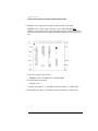
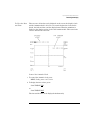
4 Build the equation by pressing:
select:, TR2, input:, build eqn, CLR - END, SEL|EDT SEL
5 Turn the front-panel to highlight the j operand, and then press:
INSERT
Continue using this technique to construct the trace equation shown in the
following figure. Enter numbers using the front-panel numeric keypad.
2-31
Application Tutorials
Tutorial 9: Constructing a Low-Pass Filter from a Transfer Function
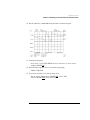
6 Build the trace equation shown in the following figure by pressing:
RETURN, select:, TR3, input:, build eqn, CLR - END, SEL|EDT SEL
Build the trace equation. Notice the cursor has wrapped to the following line.
Be sure to include the last two right parenthesis characters shown on the last
line.
7 Turn auto-scaling on by pressing:
RETURN, format:, PHASE, Scale, AUTO-SCALE
8 Set the marker by pressing:
Markers, M1 ↓
Continue pressing M1 ( ↓) until TR3 is shown in the M1 ( ↓) softkey label.
9 Repeatedly press M2 ( ↓) until TR3 is shown in the M2 ( ↓) softkey label.
Application Tutorials
Tutorial 9: Constructing a Low-Pass Filter from a Transfer Function
10 Set the marker on 1.86224 GHz using the knob or numeric keypad.
11 Continue by pressing:
Scale, more 1 of 2, AUTO DELAY, Traces, store trace, to user correct ,
adaptiv ON|OFF ON
12 Store the filter response in user-corrections by pressing:
CHAN 1 USR COR
13 To view the response or to view the data, press:
Traces, select:, TR2, display ON|OFF OFF, select:, TR3,
display ON|OFF OFF, select:, TR1, input:
2-33
Application Tutorials
Tutorial 9: Constructing a Low-Pass Filter from a Transfer Function
14 Highlight "UCORR1" using the knob.
15 Continue by pressing:
RETURN, Scale, AUTO-SCALE, page 1 of 2, Calib, user corr
Application Tutorials
Tutorial 9: Constructing a Low-Pass Filter from a Transfer Function
16 To store the filter to a memory card, press:
States, more 1 of 2, mass storage
17 If the mass-storage device needs to be selected, refer to “Saving to Mass
Storage” on page 3-34.
18 Save the user-corrections by pressing:
save, SAVE USR COR
19 To restore the instrument settings, press:
INSTR PRESET
2-35
Application Tutorials
Tutorial 10: Create a Vertical Histogram
Tutorial 10: Create a Vertical Histogram
This tutorial creates a vertical histogram on data taken from a sine wave. The
procedure, however, works for any type of waveform.
Select the Histogram Type
1 Display a trace to perform statistical analysis on.
2 Display the histogram menu by pressing:
page 1 of 2, Analyze, histogm
3 Select the trace to perform the statistical analysis on by pressing:
trace:
Use the knob to select the desired trace.
4 Select the Vertical Histogram function by pressing:
histog:, VERTICL HISTOGM VERTICL HISTOGM
Acquire the Data
5 Define the window for taking histogram data by pressing:
other, WINDOW MARKER1, WINDOW MARKER2
Notice the values of the marker positions are indicated at the top of the display.
Application Tutorials
Tutorial 10: Create a Vertical Histogram
6 Enter the number of samples to be taken for the histogram by pressing:
prev menu, NUMBER SAMPLES, # of samples, ENTER
The default number of samples taken is 1000.
7 To draw the vertical histogram, press:
SINGLE ACQUIRE
Data will be acquired once.
8 To continually acquire and update the histogram, press:
CONT ACQUIRE
2-37
Application Tutorials
Tutorial 10: Create a Vertical Histogram
Perform Statistical Analysis
The range of sample points used to calculate the mean and standard deviation
is the full screen.
9 To change the limits, press:
other, UPPER LIMIT, LIMIT→ 0%-100%, new upper limit value, ENTER,
LOWER LIMIT, LIMIT→ 0%-100%, new lower limit value, ENTER
Notice the values of the limit-line positions are indicated at the top of the display.
Application Tutorials
Tutorial 10: Create a Vertical Histogram
10 To display a line indicating the location of the mean, press:
results, MEAN,
The mean and standard deviation values are also shown.
2-39
Application Tutorials
Tutorial 10: Create a Vertical Histogram
11 To display a line indicating the location of the standard deviation, press:
STD DEV
Application Tutorials
Tutorial 11: Create a Horizontal Histogram
Tutorial 11: Create a Horizontal Histogram
This tutorial creates a horizontal histogram on data taken from a sine wave.
The procedure, however, works for any type of waveform.
Select the Histogram Type
1 Display a trace to perform statistical analysis on.
2 Display the histogram menu by pressing:
page 1 of 2, Analyze, histogm
3 Select the trace to perform the statistical analysis on by pressing:
trace:
Use the knob to select the desired trace.
4 Select the Vertical Histogram function by pressing:
histog:, HORZNTL HISTOGM HORZNTL HISTOGM
Acquire the Data
5 Define the window for taking histogram data by pressing:
other, WINDOW MARKER1, WINDOW MARKER2
Notice the values of the marker positions are indicated at the top of the display.
2-41
Application Tutorials
Tutorial 11: Create a Horizontal Histogram
6 Enter the number of samples to be taken for the histogram by pressing:
prev menu, NUMBER SAMPLES, # of samples, ENTER
The default number of samples taken is 1000.
7 To draw the horizontal histogram, press:
SINGLE ACQUIRE
Data will be acquired once.
8 To continually acquire and update the histogram, press:
CONT ACQUIRE
Application Tutorials
Tutorial 11: Create a Horizontal Histogram
Perform Statistical Analysis
The range of sample points used to calculate the mean and standard deviation
is the full screen.
9 To change the limits, press:
other, UPPER LIMIT, LIMIT→ 0%-100%, new upper limit value, ENTER,
LOWER LIMIT, LIMIT→0%-100%, new lower limit value, ENTER
Notice the values of the limit-line positions are indicated at the top of the display.
2-43
Application Tutorials
Tutorial 11: Create a Horizontal Histogram
10 To display a line indicating the location of the mean, press:
results, MEAN
The mean and standard deviation values are also shown.
Application Tutorials
Tutorial 11: Create a Horizontal Histogram
11 To display a line indicating the location of the standard deviation, press:
STD DEV
2-45
Application Tutorials
Tutorial 11: Create a Horizontal Histogram
3
Eye-Diagram Analyzer Reference
Eye-Diagram Analyzer Reference
Eye-Diagram Analyzer Reference
Eye-Diagram Analyzer Reference
In this chapter, you will find information on the following topics:
•
•
•
•
•
•
•
•
•
•
•
•
•
•
Performing Eye-Diagram Measurements 3-3
Generating Histograms 3-7
Masks and Limit Lines 3-9
Eye-Diagram Menu Maps 3-12
Agilent 70820A Menus 3-14
Controlling the Display 3-16
Calibrating the Eye-Diagram Analyzer 3-23
Displaying Traces 3-25
Using Markers 3-30
Applying Mask Testing 3-31
Saving to Mass Storage 3-34
Creating Copies of the Display 3-47
Agilent 70820A User-Corrections 3-49
Agilent 70820A Calibration 3-61
Eye-Diagram Analyzer Reference
Performing Eye-Diagram Measurements
Performing Eye-Diagram Measurements
To perform the automatic eye-diagram measurements, use the Measure menu.
With the exception of extinction ratio, these measurements must be performed in eye mode.
Automatic Measurements
The Measure menu’s top two softkeys automatically start measurements:
• EXTINCT RATIO
• MEASURE EYE
• Use the EXTINCT RATIO softkey to automatically compute the extinction ratio
in eye or eyeline modes. This measurement is a ratio of the most prevalent logical one level divided by the logical zero level over one bit interval. When making extinction ratio measurements in eyeline mode, the number of samples
should be increased from the default of 1000 to approximately 20000. This insures that a number of traces are evaluated to compute the extinction ratio.
3-3
Eye-Diagram Analyzer Reference
Performing Eye-Diagram Measurements
Use the NUMBER SAMPLES softkey for this purpose.
• Use the MEASURE EYE to initiate a number of automatic histogram measurements on an eye-diagram.
• Use the r/f tim ON OFF softkey to enable rise time and fall time measurements
during the measure eye routine. This approximately doubles the measurement
time.
• Use the UPPER THRSHLD and LOWER THRSHLD softkeys to set the upper
and lower edges for rise time and fall time measurements. These softkeys
define the amplitude level to be used for the upper and lower parts of an
edge definition for the automatic measurement functions.
• The default upper threshold is 80%. The default lower threshold is 20%.
Measurement Definitions
Extinction Ratio
This measurement is the ratio of the most prevalent high level to the most
prevalent low level over one bit interval. The measurement results are displayed in both linear and logarithmic (10log) forms of the ratio.
The peaks of the histogram are used to set initial limits for the computation of
the one and zero levels. The initial mean and sigma of the one level is based on
histogram data above the relative 50% point of the peaks. The limits for the
next evaluation of the histogram data are set to the initial mean plus-or-minus
one sigma. The new mean and sigma for the one level is determined. This process iterates several times until the sigma becomes small and the mean converges on the most prevalent one level. The determination of the most
prevalent zero level is based on the same algorithm, except the initial mean
and sigma of the zero level are based on histogram data below the relative 50%
point of the peaks.
1 Level (mean, σ)
This measurement is the mean and sigma of the one level determined from a
20% window of a bit interval centered in the middle of the bit.
0 Level (mean, σ)
This measurement is the mean and sigma of the zero level determined from a
20% window of a bit interval centered in the middle of the bit.
Eye Height
This measurement is the difference between the mean minus-three sigma of
the one level and the mean plus-three sigma of the zero level.
Eye-Diagram Analyzer Reference
Performing Eye-Diagram Measurements
Crossing Level
This measurement is the amplitude that the one level and zero level cross. It
also expresses the level as a percentage of the mean one level and mean zero
level difference.
Eye Width
This measurement is the eye width determined from the bit period and the
eye jitter. On the eye, the edges are defined to be the left crossing point plusthree sigma and the right crossing point minus-three sigma.
Eye Jitter (σ)
This measurement is the sigma of a horizontal histogram at the crossing point.
Mean Rise Time
This measurement is the mean time interval between a horizontal histogram
centered at the lower threshold point and a horizontal histogram centered at
the upper threshold point on a rising edge of an eye-diagram.
Mean Fall Time
This measurement is the mean time interval between a horizontal histogram
centered at the upper threshold point and a horizontal histogram centered at
the lower threshold point on a falling edge of an eye-diagram.
Measure Fast Amplitude and Phase Transitions
The 70820A module measures fast amplitude and phase transitions on continuous wave (CW) and modulated signals. Time, frequency, and power sweeps
can be performed from dc to 40 GHz. The 70820A module triggers on the RF
input signal.
During stimulus/response measurements, the 70820A module controls an RF
source instrument’s:
• frequency
• power
• pulse modulator
Viewing Repetitive and Non-Repetitive Signals
Because of the sampling techniques employed by the 70820A, the 70820A
module is optimized for viewing repetitive input signals. However, there is single-shot operation for viewing baseband and modulated non-repetitive signals
having bandwidths up to 10 MHz. Pre-trigger data can also be viewed. An
example of using the single shot operation is measuring the turn-on characteristics of a pulse modulator. Single shot operation uses a maximum sampling
rate of 20 MHz.
3-5
Eye-Diagram Analyzer Reference
Performing Eye-Diagram Measurements
For Optimum Performance
The 70820A module should be configured to:
• Control the RF source over the communications bus.
• Share the same frequency reference as the RF source.
Channels Versus Traces
The 70820A module has two input channels, four traces, and four trace memory registers.
• Channels are used to measure input signals.
• Traces are used to display measurement results.
• Trace memory registers can be used as a third channel.
Eye-Diagram Analyzer Reference
Generating Histograms
Generating Histograms
The 70820A can perform statistical analysis on any displayed trace. After creating a vertical or horizontal histogram of the trace data, the display can show
mean and standard deviation values of the histogram.
Histogram analysis is performed using the Histogram menu.
Press:
MENU, the left-side page 1 of 2, Analyze, Histogm
The 70820A menus perform vertical or horizontal histograms on any single
trace
You can control the number of samples taken, the window for valid data samples, and the sample bounds for calculating mean and standard deviations
The Histogram Menu
3-7
Eye-Diagram Analyzer Reference
Generating Histograms
When generating histograms, you must perform the following basic steps:
1 Select a trace.
2 Select histogram type.
3 Enter the number of samples.
4 Set limits for acquired data.
5 Acquire the data.
6 Establish limits for statistical analysis.
7 View the mean and standard deviation.
Histogram data can be acquired once using the SINGLE ACQUIRE softkey or
continuously updated using the CONT ACQUIRE softkey.
Press other for this additional menu.
Eye-Diagram Analyzer Reference
Masks and Limit Lines
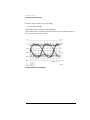
Masks and Limit Lines
Masks and limit lines allow you to test the shape (time or frequency versus
amplitude) of a displayed response. Masks are closed polygon shapes. Limit
lines are lines. Traces or measurement points that penetrate a mask or cross a
limit line result in testing errors.
Two Masks Displayed on Screen
3-9
Eye-Diagram Analyzer Reference
Masks and Limit Lines
A Limit Line Displayed on Screen
Because you can perform repetitive testing of response shapes, masks and
limit lines are ideal for pass/fail testing on production lines. You create, save,
recall, and edit limit lines using the masks, limits menu. Access this menu
using the left-side Analyze softkey.
Since masks and limit lines are treated similarly, in this chapter, most references to masks applies equally to limit lines.
Eye-Diagram Analyzer Reference
Masks and Limit Lines
Testing Responses
Once you’ve created a mask or limit line, set the following conditions for testing:
• Trace to which testing is applied.
• Violations defined as traces or measurement points.
• Testing ends after a set number of errors.
• Testing ends after a set number of traces.
Use the test ON|OFF softkey to start testing. Testing stops whenever one of
the following events occurs:
• A set number of trace sweeps.
• A set number of violations.
• test ON|OFF is set to OFF.
Numbers displayed at the bottom of the screen indicate the number of violations and trace sweeps that have occurred. The following figure shows a
response that has violated a limit line three times on three sweeps.
3-11
Eye-Diagram Analyzer Reference
Eye-Diagram Menu Maps
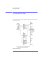
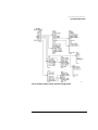
Eye-Diagram Menu Maps
The two menu maps in this section graphically represent the eye-diagram analyzer’s softkey menus.
Setup and Trg, Cal Menus
Eye-Diagram Analyzer Reference
Eye-Diagram Menu Maps
Traces, Measure, Markers, Masks, and Mass Storage Menus
3-13
Eye-Diagram Analyzer Reference
Agilent 70820A Menus
Agilent 70820A Menus
This section discusses the softkey menus for the 70820A microwave transition
analyzer module. To learn about the eye-diagram analyzer’s menus, refer to
“Eye-Diagram Menu Maps” on page 3-12. These menus provide additional features useful for running the eye-diagram analyzer.
You will find the preview feature discussed in this chapter very useful. It displays the programming command, corresponding to the response received,
when most softkeys are pressed.
Most front-panel controls are accessed via softkey menus. Softkeys are the
seven buttons located on each side of the screen. The functions of softkeys
change according to the menus displayed on the screen.
Page 1 of Top Level Menus
Eye-Diagram Analyzer Reference
Agilent 70820A Menus
The Left-Side Softkeys
Use the softkeys located on the left side of the display to access the twelve
major menus. These softkeys are shown in two pages. Press page 1 of 2 to view
the second page of softkeys. When the 70820A module first turns on, the Main
menu is automatically selected.
Page 2 of Top Level Menus
3-15
Eye-Diagram Analyzer Reference
Controlling the Display
Controlling the Display
To Control the
Number of Bits
Displayed
The Setup menu’s BIT INTVL softkey allows you to select the number of bits
that will be displayed on the screen. The horizontal time scale automatically
changes to the appropriate setting. Use DELAY to enter time delay. The
amount of delay is entered in bits. Use this feature, in pattern mode, to view
different portions of the PRBS waveform.
The amount of delay can be as much as 1000 times the time span. In addition,
the eye-diagram analyzer can view the trace before the trigger event. Negative
time delay up to {-time span}over2 can be entered.
Set the number of bits displayed by pressing:
Setup, BIT INTVL and enter the number of bits to display.
Set the time delay by pressing:
Setup, DELAY and enter the desired time delay
To Measure in
Optical Power
Units
The Trg, Cal menu’s CH1 EXT ATTEN and CH2 EXT ATTEN softkeys allow
you to specify any external attenuation or optical-to-electrical responsivity
conversion between the source and input channels. Specifying an attenuation
on channel 1 changes the measurement plane from the front-panel channel 1
connector to include the indicated attenuation. Specifying an optical-to-electrical responsivity displays optical units referenced to the input of the opticalto-electrical converter. Channel and marker readouts change to watts/div.
Also, the CH1 EXT ATTEN softkey changes to read CH1 RSPVTY (responsivity).
To measure the optical power, press:
Trg, Cal, CH1 EXT ATTEN and enter the responsivity value in watts/div
Notice the CH1 EXT ATTEN softkey changes to read CH1 RSPVTY (responsivity).
Eye-Diagram Analyzer Reference
Controlling the Display
To Improve the
Sensitivity in
Eyeline Mode
In eyeline mode, additional eye filtering can be applied to improve the measurement sensitivity. This can be an advantage when measuring extinction
ratios on low-level signals. Use the eyefltr ON OFF softkey to apply the filter.
When the pattern repetition frequency is greater than 10 MHz, internal filtering is applied that provides a 20 dB signal-to-noise improvement. For pattern
repetition frequencies less than 10 MHz, software filtering is applied that
allows variable signal-to-noise improvement versus sweep time.
To improve sensitivity, press:
Setup, diagram, EYELINE or PATTERN, eyefltr ON OFF ON
Use the front-panel knob to adjust the amount of filtering applied.
To Extend the
Bandwidth to 40
GHz
Use the extd BW ON OFF softkey to enable RF corrections which extend the
measurement bandwidth of the eye-diagram analyzer to 40 GHz. Extended
bandwidth operation can be used in both eyeline and pattern modes, but not
in eye mode.
1 Extend the measurement bandwidth by pressing:
Setup, diagram, EYELINE or PATTERN
The extended 40 GHz bandwidth cannot be used in eye mode.
2 Turn the extended bandwidth on by pressing:
Trg, Cal, more 1 of 2,, extd BW ON|OFF ON
To Apply UserCorrections
User-corrections provide a convenient method for modifying the display of
input signals. Some of the applications for user-corrections include the following:
• Filtering input signals to simulate the effects of circuit design.
• Compensating for frequency and phase response of external probes.
• Compensating for frequency and phase response of external test setups.
• Compensating for the frequency response of optical to electrical converters.
Several Bessel-Thomson software filters are included on the 70874A eye-diagram analyzer’s memory card. These filters can be applied as user-corrections
in the eyeline and pattern modes. (User corrections must be off in eye mode.)
User correction files are identified by the prefix a_ as shown in the following
table. The files AUTOST and 70874 comprise the eye-diagram analyzer program.
3-17
Eye-Diagram Analyzer Reference
Controlling the Display
To learn more about these files and about creating and applying user-corrections, refer to “Tutorial 5: Use Software Filters” on page 2-15.
User-Correction Files
File Name
File Data
a_bt248832
4th order Bessel- Thomson filter for 2.48832 Gbit/sec transmission.
a_bt_62208
4th order Bessel- Thomson filter for 622.08 Mbit/sec transmission.
a_bt_15552
4th order Bessel- Thomson filter for 155.52 Mbit/sec transmission.
1 Place the 70874A eye-diagram analyzer memory card in the front-panel card
slot.
The 70874A eye-diagram analyzer must already be loaded into memory.
2 Display the eye-diagram analyzer’s menus by pressing:
USER, Setup, diagram, EYELINE or PATTERN
User corrections can not be applied in eye mode.
3 Display a catalog of the files contained on the memory card by pressing:
Mass Storage
Rotate the front-panel knob to highlight the desired file.
User correction files are identified by the prefix a_.
Eye-Diagram Analyzer Reference
Controlling the Display
4 Load the file by pressing:
LOAD FILE
The file is loaded when user-corrections loaded is displayed on the
screen.
5 Turn the user correction function on by pressing:
Trg, Cal, more 1 of 2, usr cor ON|OFF ON.
3-19
Eye-Diagram Analyzer Reference
Controlling the Display
User-Corrections Applied to the Data
To View 70820A
Menus
Press MENU.
To Return to the
Jitter Analyzer
(or Eye-Diagram
Analyzer)
Press USER.
To Preview
Programming
Commands
Press MENU, Config, more 1 of 3, preview ON|OFF ON
To View the
Firmware Date
Code
If the eye-diagram analyzer’s menus are not displayed, load the program as
explained in Chapter 1, “Getting Started”.
For a demonstration of the Preview function, press persist ON|OFF. Notice the
corresponding programming command DISP:PERS 1024 is displayed at the
bottom of the screen.
Press MENU, Config, more 1 of 3, more 2 of 3, system, ROM VERSION
Eye-Diagram Analyzer Reference
Controlling the Display
To View the Date
and Time
There are two clocks that can be displayed on the screen: the display’s clock
and the 70820A module’s clock. You can control whether the clocks are displayed, the indicated time, and the display format. When the mainframe is
turned on, the display sets the clock in the 70820A module. This causes both
clocks to indicate the same time.
Control the 70820A’s Clock
1 To control the 70820A’s clock, press:
MENU, Config, more 1 of 3, clock
2 To display the time or date, press:
show TIM|DAT TIM
or:
show TIM|DAT DAT
The time and the date can be displayed simultaneously.
3-21
Eye-Diagram Analyzer Reference
Controlling the Display
3 To select US or European display format, press
US|EURO US
or:
US|EURO EURO
4 To change the time or date, press:
set clock
Enter the new value in the same format as displayed.
Control the Display’s Clock
1 Press DISPLAY, Misc, clock
• If you want to turn the clock display on and off, press CLOCK DISPLAY.
• If you want to select US or European display format, press US/EURO.
• If you want to change the time or date, press set clock.
2 Enter the new value in the same format as displayed.
Eye-Diagram Analyzer Reference
Calibrating the Eye-Diagram Analyzer
Calibrating the Eye-Diagram Analyzer
Note
For information on user-corrections and instrument calibration data, refer to
“Agilent 70820A User-Corrections” on page 3-49 and refer to “Agilent 70820A
Calibration” on page 3-61.
To Compensate
for dc Offsets
An offset calibration routine is provided that allows the eye-diagram analyzer
to compensate channel 1 for any external or internal dc offsets. This ensures
accurate measurements of the laser’s one and zero levels. For example, you
can use the calibration to remove any offset that may be present in an opticalto-electrical converter. This is sometimes referred to as the "dark" level.
To perform an offset calibration
1 Turn the laser off and then press:
Trg, Cal, OFFSET CAL, CONT
The calibration takes about a minute to execute. When the calibration is
finished, DC NULL: done is displayed.
2 Turn the laser on.
To Calibrate IF
for Accuracy
The 70820A microwave transition analyzer module provides separate automatic IF calibration routines for channel 1 and channel 2. Each requires
approximately 30 minutes to run. For optimum performance, you should perform the calibrations when at least one of the following is true:
• The temperature has changed ±5° Centigrade since the last calibration was
performed.
• More than one week has passed since the last calibration.
• Before any critical measurement.
CAUTION
Allow the microwave transition analyzer module to warm up for at least one
hour before performing a calibration.
3-23
Eye-Diagram Analyzer Reference
Calibrating the Eye-Diagram Analyzer
1 Connect a low-loss cable between the front-panel CALIBRATOR OUTPUT and
channel 1 connectors.
2 To calibrate the IF, press:
MENU, page 1 of 2, Calib, IF calib, CAL CH1
The calibration routine takes about 30 minutes to complete.
3 Disconnect the cable from channel 1, and connect it to the channel 2
connector.
4 Repeat the above procedure for channel 2.
Eye-Diagram Analyzer Reference
Displaying Traces
Displaying Traces
Four Traces can be Displayed
The Traces menu’s select: softkey allows you to display and control up to four
traces. The scaling, reference positions, and reference levels of each trace can
be separately adjusted. To automatically adjust the trace scale factor and reference level for optimum display, simply press AUTO-SCALE. Signals are
autoscaled once when the softkey is pressed and not on a continual basis. If
you change the amplitude of the signal, it will not be autoscaled.
During mask testing, trace 4 is reserved for the error trace.
To Display a Trace
Press Traces, select:, TR1, TR2, TR3, or TR4, display ON OFF ON
3-25
Eye-Diagram Analyzer Reference
Displaying Traces
To Position and
Scale Each Trace
The selected trace can be positioned vertically on the display. This is accomplished using the REF LEV|POS softkey to enter both the reference position and
reference level. The reference position (POS) is entered as a percentage of the vertical display. The top of the screen is 100%. The bottom of the screen is 0%. The reference level (REF LEV) is the amplitude value at the reference position.
To scale and position a trace, press:
Traces, AUTO-SCALE to automatically scale the selected trace.
or
SCALE to manually set the scale.
Use the front-panel knob or numeric keypad to change the displayed vertical
scaling.
REF LEV|POS POS to move the trace’s reference position.
Rotate the front-panel knob to change the position.
REF LEV|POS LEV to change the reference level at the trace’s reference
position.
Rotate the front-panel knob to change the level.
To Average Trace
1
The Traces menu’s average softkey presents a menu used for controlling trace
averaging. Trace averaging keeps a running average of the measurement values on each sweep. You can set the averaging count; its default value is 16.
Trace averaging is only applied to trace 1.
Eye-Diagram Analyzer Reference
Displaying Traces
The Averaging Submenu
Average trace 1 by pressing:
Traces, average, AVERAGE SWEEPS and enter the number of sweeps used
for running average, average ON|OFF ON
Four Persistence Modes are Available
The eye-diagram analyzer offers four trace persistence selections. These
selections are located under the Traces menu’s persist softkey and include the
following types:
• Infinite monochrome
• Variable monochrome
• Color grading
• Monochrome grading
Trace persistence works on all displayed traces regardless of which trace is
selected.
3-27
Eye-Diagram Analyzer Reference
Displaying Traces
The Persistence Submenu
Infinite Monochrome Persistence
With infinite monochrome persistence ( INFINIT), traces accumulate on the
display until persistence is turned off or the display is cleared using the Setup
menu’s CLEAR DISPLAY softkey. Press OFF to turn off infinite monochrome
persistence.
Variable Monochrome Persistence
With variable monochrome persistence ( VARIABL), older traces become dimmer as new traces are acquired. Traces can be one of seven different brightness levels, with new traces being the brightest. After N number of sweeps (N
is set with the PERSIST SWEEPS), every trace gets dimmer by one intensity
level; traces already at the dimmest level disappear altogether. Lower values
of N work best with this type of persistence, typically values of five through
10. Press OFF to turn off this persistence.
Color Grading Persistence
With color grading persistence ( COLOR GRADING), the color of a displayed
pixel is a function of how many times a trace dot falls on that particular pixel.
There are five possible colors that a pixel can be. If a pixel has progressed to
the highest color (yellow) before N PERSIST SWEEPS have occurred, it
remains that color no matter how many more dots fall on it. After N PERSIST
SWEEPS, the color grading acquisition stops. The following list shows the
order of colors a pixel can progress through:
Eye-Diagram Analyzer Reference
Displaying Traces
1 green
2 cyan (light blue)
3 purple
4 rose
5 yellow
This persistence works best with high values of N, typically values of 50
through 100. In this mode, no softkeys can be pressed until after EXIT GRADING is pressed.
Monochrome Grading Persistence
Monochrome grading persistence ( MONO GRADING) works just like color
grading except that a given pixel increases in intensity instead of color each
time a dot falls on it. There are 15 different levels of intensity. In this mode,
EXIT GRADING must be used to return to normal instrument operation.
a Apply persistence by pressing:
Traces, persist, PERSIST SWEEPS
Enter one of the following:
• If variable persistence will be used, enter the number of sweeps taken before
a trace decrements in brightness.
• If grading persistence will be used, enter the number of sweeps taken until
the grading display is stopped.
b Press one of the four top right-side softkeys to select the persistence mode.
c Pressing OFF can stop INFINIT and VARIABLE persistence at any time.
3-29
Eye-Diagram Analyzer Reference
Using Markers
Using Markers
Use this menu to activate the four available line markers: X1, X2, Y1, and Y2.
Markers allow you to measure or compare portions of the displayed waveform.
For example, you can use markers to measure the peak-to-peak difference in a
laser’s turn-on time as measured on the eye-diagram’s crossing point.
Use the front-panel knob or numeric keypad to position each displayed
marker on the screen. Notice that the value at the marker is displayed on the
top portion of the screen. To turn the markers off, simply press MARKERS
OFF.
Eye-Diagram Analyzer Reference
Applying Mask Testing
Applying Mask Testing
Use the Masks menu to display and control mask testing. Built in standard
masks for the more common SONET/SDH transmission rates are provided. To
learn how to create your own custom masks, refer to Chapter 2, “Application
Tutorials”.
Test Results are Displayed
During mask testing, mask violations are displayed in the lower portion of the
display. You can specify whether the mask errors are counted as trace errors
or as the number of trace points or dots that violated the mask. You do this
using the count TRC|DOT softkey.
3-31
Eye-Diagram Analyzer Reference
Applying Mask Testing
Automatic Alignment Scales the Mask
The MASK ALIGN softkey, located under the Masks menu, automatically
aligns and scales a default mask to the data per the SONET/SDH standards.
This is accomplished using histograms and is best done in eye mode for faster
and more evenly distributed data acquisition. Eye mode provides a more even
statistical distribution of high and low data. This results in faster acquisition of
the histogram data used to determine zero and one levels. The mask and limit
lines adjust to fit the displayed data. To change the number of samples used
for the histogram, use the Measure menu’s NUMBER SAMPLES function.
Display the Error Trace
Use the err trc ON OFF softkey to display a trace that violates a mask. The
screen is split with the error trace displayed in the lower half of the display.
Trace four is allocated as the error trace.
Mask Margins Tighten Mask Tests
Margins can be added to the mask/limit line tests. This margin is added as a
percent of the mask. Zero percent margin corresponds to the default mask.
One hundred percent margin corresponds to the mean of the histograms of
the one and zero levels, and the crossing points.
Negative mask margins can also be implemented. These can be used to gain an
idea of time severity of the encountered errors.
Eye-Diagram Analyzer Reference
Applying Mask Testing
The Mask Setup Submenu
3-33
Eye-Diagram Analyzer Reference
Saving to Mass Storage
Saving to Mass Storage
Use the Mass Storage menu, to save and recall files to a mass storage device.
The mass storage device is normally a memory card that has been inserted
into the front-panel card slot. You can also store data to a GPIB disk drive, and
to internal random-access memory (RAM) disk, refer to “Selecting and Formatting Memory” on page 3-34.
Each file that you save has a name that consists of a prefix followed by a custom name that you enter. The analyzer assigns a prefix according to the type
of data. Refer to “Working with Files” on page 3-40.
The following list shows the types of data that can be saved as files:
•
•
•
•
•
•
•
•
•
•
Traces
Measurement states
Histograms
Masks
Limit lines
Calibrations
User corrections
User menus
Downloadable programs (DLPs)
Jitter template and calibration files
Selecting and Formatting Memory
When first turned on, the microwave transition analyzer module automatically
selects the memory card as the mass-storage device. You can format memory
and save, recall, erase, and list (catalog) files using the mass-storage menu
located in the States menu.
Memory Cards
Memory cards must be formatted before use. Formatting erases any previously stored files and initializes memory for storing data. RAM memory cards
have a built-in battery to retain memory data. Data stored in the card remain
Eye-Diagram Analyzer Reference
Saving to Mass Storage
as long as the card’s battery has sufficient power. You should change the battery every two years using the procedure in this section. Refer to “To Change a
Memory Card Battery” on page 3-39.
RAM memory cards have a write-protect switch, on the end which is not
inserted into the display’s card slot. If this switch is slid toward the edge of the
card (marked "SAFE"), no changes may be made to the card’s content. If you
wish to write a new file to a card, or remove a file, slide its write-protect switch
toward the center of the card.
Note
If no card is inserted in the front-panel card slot, and you attempt to catalog a
memory card, the display shows the message catalog open failed. Place a card
in the card slot, and retry the operation.
RAM Disks
RAM disks offer a convenient method of duplicating memory cards. Refer to
“To Duplicate a Memory Card” on page 3-41. Up to 16 internal RAM disks can
be created. (These are numbered 0 through 15.) The default size of each RAM
disk is 32 kilobytes.
Use Instrument BASIC’s INITIALIZE statement to create each disk. The following example creates RAM disk zero:
INITIALIZE ":MEMORY,0,0",128
The second integer, 0, determines the RAM disk number. The value 128 represents the size of the RAM disk in sectors. Each sector consists of 256 bytes.
So, a value of 128 sectors creates a RAM disk of 32 kilobytes. A value of 512
sectors creates a RAM disk of 128 kilobytes.
Use the following command to create RAM disk 1 with a size of 128 kilobytes:
INITIALIZE ":MEMORY,0,1",512
CAUTION
Because internal RAM is volatile, all RAM disks are deleted when the power is
turned off. When this happens, all files are lost and each RAM disk must be
recreated.
3-35
Eye-Diagram Analyzer Reference
Saving to Mass Storage
GPIB Disk Drives
Measurement data and files can be saved on an external GPIB disk drive. The
disk drive must be a 3.5 inch, CS80 compatible, such as an 9122. To use the
drive, you must connect it and enter its GPIB address using DISPLAY menu
softkeys. The procedure in this section shows you how to do this. You will
need to know the disk drive’s GPIB address, unit number, and volume number.
The GPIB address is represented by a digit from 1 through 7. The unit number
indicates an individual slot in the disk drive. Although unit numbers can range
from 0 through 9, they are typically 0 or 1. The volume number is used for
hard disk drives. For reading diskettes, the volume number should be 0.
To Use a Memory
Card
1 Insert the memory card into the front-panel card slot of the microwave
transition analyzer, facing the metal strip on the card downward and toward
the instrument. Make sure the card is fully inserted into the card slot.
2 Select the memory card as the mass storage device by pressing:
DISPLAY, Mass Storage, msi:, MEMORY CARD
3 To display a catalog of the files on the memory card, press:
MENU, page 1 of 2, States, more 1 of 2, mass storage, msi:,
HP-MSIB CARD
If the message "6218 catalog open failed" is displayed, the card is not
in the front-panel card slot. The HP-MSIB address for the card is the same
address as the display’s GPIB address and is normally set to 4. If the address is
not correct, enter the correct address using the numeric keypad.
Eye-Diagram Analyzer Reference
Saving to Mass Storage
Initializing (formatting) a memory card
CAUTION
The following steps erase any files stored on the card.
1 If the memory card is new and needs to be formatted, press:
MENU, page 1 of 2, States, more 1 of 2, mass storage, more, FORMAT
2 To use the LIF format, press:
FORMAT as LIF
3 To format as DOS, press:
FORMAT as DOS
To Use an Internal
RAM Disk
1 To invoke Instrument BASIC, press:
USER
If the eye-diagram personality is loaded, press USER again.
2 Enter an INITIALIZE statement to create a RAM disk. For example, enter the
following BASIC statement:
INITIALIZE ":MEMORY,0,0",128
3 Select the internal RAM disk by pressing:
MENU, page 1 of 2, States, more 1 of 2, mass storage, msi:, MEMORY
The RAM disk number is shown on the screen. Use the front-panel knob to
change the RAM disk number.
To Use an GPIB
Disk Drive
1 Connect the GPIB disk drive to the 70004A color display using an GPIB cable.
2 Determine or set the GPIB address of the disk drive. Refer to the disk drive’s
user’s manual for information on determining the disk drive’s address.
3 Set the GPIB address of the disk drive by pressing:
DISPLAY, Mass Storage, msi:, GPIB disk, GPIB ADDRESS
enter the address of the disk drive
This value is between 1 and 7.
3-37
Eye-Diagram Analyzer Reference
Saving to Mass Storage
4 Enter the disk drive’s unit number by pressing:
UNIT NUMBER
This number is typically a 0 or 1. Zero usually indicates the disk drive’s left
side slot.
5 Enter the disk drive’s volume number by pressing:
VOLUME NUMBER
The volume number should be left at the default value of zero for floppy disk
drives.
6 Continue by pressing:
MENU, page 1 of 2, States, more 1 of 2, mass storage, msi:,
HP-MSIB CARD
Although CARD is selected, the display’s GPIB disk softkey, pressed in Step 3 ,
redirected communications to the GPIB disk drive.
Eye-Diagram Analyzer Reference
Saving to Mass Storage
To Change a
Memory Card
Battery
The memory card’s battery is a lithium commercial CMOS type, part number
CR 2016.
The memory card should be installed when the battery is removed. If the battery is removed while the card is not installed, all data in the card will be lost.
Store memory-card files on another device before changing the battery, when
extra care is appropriate.
1 Install the memory card into the 70004A display.
2 On the front edge of the card, locate the groove of the battery clip.
3 Gently pry the battery clip out of the card. The battery fits inside the clip.
4 Replace the battery, making sure the plus (+) sign on the battery is on the same
side as the plus sign on the clip.
5 Insert the battery clip into the memory card, holding the clip as oriented in the
figure. (Face the open edge of the clip toward the memory card’s write-protect
switch.)
6 Write the date the battery was replaced on the card.
3-39
Eye-Diagram Analyzer Reference
Saving to Mass Storage
Working with Files
Files are identified by a prefix and a name. The eye-diagram analyzer assigns a
prefix according to the type of data, as shown in the following table. You enter
the file name. When cataloged, the file listings show the file’s data type and
size in bytes.
File Prefixes
File Type
File Prefix
Calibration data
c_
Histograms
h_
Instrument registers
r_
Instrument state
s_
Mask/Limit line
m_
Program
d_
Trace
t_
User corrections
a_
User menu
k_
Jitter template
T-
You can create additional prefix text for your file names. The text, appended
to the standard prefixes, allows you to indicate files that have similar data. For
example, the following figure shows a catalog of two mask files. Each file has
an additional prefix of Shape. The additional prefix is appended, regardless of
the type of file you are saving.
The total length of your file name cannot exceed 10 characters for LIF and 8
characters for DOS. This includes prefix and file name.
Eye-Diagram Analyzer Reference
Saving to Mass Storage
To Duplicate a
Memory Card
Instrument BASIC provides the ability to mass copy all the files from one
memory card to another memory card. This allows you to easily reproduce
copies without having to copy the files one at a time. Use the following steps:
1 Refer to “To Use a Memory Card” on page 3-36 to select the memory card for
use.
2 Insert the memory card with the files into the front-panel card slot.
3 Press USER. (If the eye-diagram analyzer personality is loaded, press USER
twice.)
4 Use a keyboard to enter the following Instrument BASIC commands. These
commands initialize a RAM disk and copy the files from the card to the RAM
disk. If you don’t have a keyboard, Instrument BASIC has an editor for creating
these commands.
INITIALIZE ":MEMORY,0,0"
WILDCARDS DOS
COPY "*" TO ":MEMORY,0,0"
5 Remove the card from the card slot and insert a blank formatted card in the
slot.
3-41
Eye-Diagram Analyzer Reference
Saving to Mass Storage
6 Issue the following Instrument BASIC command to copy the files from the RAM
disk to the new card:
COPY "*:MEMORY,0,0" TO ":EXTERNAL,904"
To Catalog all
Files
Use this procedure to catalog default memory. To select default memory, refer
to “Selecting and Formatting Memory” on page 3-34.
1 If you plan to catalog the files on a memory card, insert the card in the frontpanel card slot.
2 Display a catalog of the files by pressing:
MENU, page 1 of 2, States, more 1 of 2, mass storage
Remember to insert the card before cataloging a memory card. If the message
"6218 catalog open failed" is displayed, the card is missing. The HPMSIB address for the card is the same address as the display’s GPIB address
and is normally set to 4. If the address is not correct, enter the correct address
using the numeric keypad.
To Save a File
Use this procedure to save a file in the default memory. To select default memory, refer to “Selecting and Formatting Memory” on page 3-34.
1 Display the Mass Storage menu by pressing:
MENU, page 1 of 2, States, more 1 of 2, mass storage, save
2 Perform one of the following:
• If you are saving an instrument state, user-correction, or histogram, press the
appropriate softkey.
• If you are saving a trace, press save trace. Select the trace and then use the
VEC|FMT softkey to determine if the trace data is saved as complex data
(VEC) or scalar data (FMT). Press save.
• If you are saving a channel calibration, mask, limit line, user-defined key, all
recall registers, press save misc and then the appropriate softkey.
3 Enter the desired file name.
4 To save the file, press:
ENTER LINE
An HP-IL keyboard is recommended to simplify the task of entering alphanumeric information. This keyboard plugs into the jack provided on the display’s
front panel. Order the Agilent 46021A keyboard.
Eye-Diagram Analyzer Reference
Saving to Mass Storage
Entering a File Name without a Keyboard
a Turn the front-panel knob to move the character-select cursor.
b Press SELECT CHAR to enter a character at the character-select cursor.
c Press the numeric keypad to enter numbers or a minus sign.
d The INSERT or ... softkey determines the action of the SELECT CHAR softkey. Choices are INSERT a character, REPLACE an existing character, or
DELETE a character.
e Press the ⇑ and ⇓ keys (beneath the front-panel knob) to move the command-entry cursor.
f Use the CLEAR TO END softkey to remove characters from the commandentry cursor to the end of the command.
To Recall a File
Use this procedure to recall a file from the default memory. To select default
memory, refer to “Selecting and Formatting Memory” on page 3-34.
1 To recall a file, press:
MENU, page 1 of 2, States, more 1 of 2, mass storage
Rotate the front-panel knob to select (highlight) the desired file.
2 Load the file by pressing:
LOAD FILE
To Erase a File
Use this procedure to erase a file in the default memory. To select default
memory, refer to “Selecting and Formatting Memory” on page 3-34.
1 To erase a file, press:
MENU, page 1 of 2, States, more 1 of 2, mass storage
Rotate the front-panel knob to select (highlight) the desired file.
2 To erase the file, press:
more, PURGE FILE, ENTER LINE
3-43
Eye-Diagram Analyzer Reference
Saving to Mass Storage
To Erase all Files
CAUTION
This procedure erases all files stored in default memory.
To erase all files in default memory, press:
MENU, page 1 of 2, States, more 1 of 2, mass storage, more, FORMAT
To Change the
Prefix
1 To modify the prefix, press:
MENU, page 1 of 2, States, more 1 of 2, mass storage, more, CHANGE
PREFIX
Enter the desired text.
2 To enter the prefix, press:
ENTER LINE
Entering the prefix without a keyboard
a Turn the front-panel knob to move the character-select cursor.
b Press SELECT CHAR to enter a character at the character-select cursor.
c Press the numeric keypad to enter numbers or a minus sign.
d The INSERT or ... softkey determines the action of the SELECT CHAR softkey. Choices are INSERT a character, REPLACE an existing character, or
DELETE a character.
e Press the ⇑ and ⇓ keys (beneath the front-panel knob) to move the command-entry cursor.
f Use the CLEAR TO END softkey to remove characters from the commandentry cursor to the end of the command.
Eye-Diagram Analyzer Reference
Saving to Mass Storage
To Erase a Custom
Prefix
1 To erase a custom prefix, press:
MENU, page 1 of 2, States, more 1 of 2, mass storage, more, CHANGE
PREFIX
Repeatedly press the ⇓ step key until the cursor is located at the start of the
custom text.
2 Clear the text by pressing:
CLEAR TO END, ENTER LINE
To Save an
Instrument State
1 Set the eye-diagram analyzer to the desired settings.
2 Insert a ROM card into the front-panel card slot.
3 Save the instrument state by pressing:
Mass Storage, SAVE STATE
To Load a State or
Mask/Limit Line
1 Insert a ROM card into the front-panel card slot and then press:
Mass Storage
Rotate the front-panel knob to highlight the desired file.
The prefix "S_" identifies instrument state files.
The prefix "M_" identifies mask/limit line files.
2 Load the file by pressing:
LOAD FILE
3-45
Eye-Diagram Analyzer Reference
Saving to Mass Storage
To Save a Mask/
Limit Line File
1 Display the Mass Storage menu by pressing:
States, more 1 of 2, mass storage
If the mass-storage device needs to be selected, refer to “Selecting and Formatting Memory” on page 3-34.
2 Enter the file name by pressing:
save, save misc, SAV MSK LIM
Use the softkeys, knob, numeric keypad, and step keys to enter the file name.
3 Save the file by pressing:
ENTER LINE
To Recall a Mask/
Limit Line File
1 To recall a mask/limit line file, press:
MENU, page 1 of 2, States, more 1 of 2, mass storage
If the mass-storage device needs to be selected, refer to “Selecting and
Formatting Memory” on page 3-34.
2 Rotate the front-panel knob to select (highlight) the desired file.
3 Load the file by pressing:
LOAD FILE
To Erase a Mask
File/Limit Line
File
1 To erase a mask/limit line file, press:
MENU, page 1 of 2, States, more 1 of 2, mass storage
If the mass-storage device needs to be selected, refer to “Selecting and
Formatting Memory” on page 3-34.
2 Rotate the front-panel knob to select (highlight) the desired file.
3 Erase the file by pressing:
more, PURGE FILE
Eye-Diagram Analyzer Reference
Creating Copies of the Display
Creating Copies of the Display
Often, it is important to create hard copies of the display for reports or
records. A copy of the display can be printed on any Hewlett-Packard graphics
printer. These printers support the Hewlett-Packard PCL printer language and
include the following:
• ThinkJet
• PaintJet
• LaserJet
Note
The printer must have an GPIB interface.
Hard copies can be produced on a Hewlett-Packard plotter if the eye-diagram
analyzer is in pattern mode. Plots cannot be produced in eye or eyeline modes.
To Create a Print
1 Connect the printer to the display via an GPIB cable.
Be sure to connect the GPIB to the display’s connector, not to the connector
on the 70820A microwave transition analyzer module.
2 The first time the printer is used, enter the printer type and address by
pressing:
DISPLAY, Hard Copy, printer address
GPIB TLK/LSN to configure the printer in talk/listen mode on the GPIB.
GPIB L ONLY to configure the printer in listen only mode on the GPIB.
To configure the printer via the HP-MSIB, use the HP-MSIB COLUMN and
HP-MSIB ROW softkeys to enter the printer address.
3 To select the type of printer used, press:
←, printer config
Use the softkeys along the right side of the display to select the printer type.
3-47
Eye-Diagram Analyzer Reference
Creating Copies of the Display
4 Select the print option by pressing:
←, copy options, COPY IS PRT/PLT PRT
5 Create the print by pressing:
USER, PRINT
To Create a Plot
Hard copies can be produced on an Hewlett-Packard plotter if the eye-diagram analyzer is in pattern mode. Plots cannot be produced in eye or eyeline
modes.
1 Connect the plotter to the display via an GPIB cable.
Be sure to connect the GPIB to the display’s connector, not to the connector
on the 70820A microwave transition analyzer module.
2 The first time the plotter is used, enter the plotter type and address by
pressing:
DISPLAY, Hard Copy, plotter address
HP-IB TLK/LSN to configure the plotter in talk/listen mode on the GPIB.
HP-IB L ONLY to configure the plotter in listen only mode on the GPIB.
To configure the plotter via the HP-MSIB, use the HP-MSIB COLUMN and HPMSIB ROW softkeys to enter the plotter address.
3 To select the type of plotter used, press:
←, plotter config
Use the softkeys along the right side of the display to select the plotter type.
4 Select the plotter option by pressing:
←, copy options, COPY IS PRT/PLT PLT
5 Create the plot by pressing:
USER, PLOT
Eye-Diagram Analyzer Reference
Agilent 70820A User-Corrections
Agilent 70820A User-Corrections
User corrections provide a convenient method for modifying the display of
input signals. Some of the applications for user-corrections include the following:
• Filtering input signals to simulate the effects of circuit design.
• Compensating for frequency and phase response of external probes.
• Compensating for frequency and phase response of external test setups.
• Compensating for the frequency response of optical to electrical converters.
To create and use your own user-corrections, enter the User Correction menu.
(This menu is located under the 70820A’s Calib menu.) The microwave transition analyzer maintains two separate user-correction memories: one for channel 1 and one for channel 2. After entering the User Correction menu, the
microwave transition analyzer displays user-correction data in the lower half
of the screen. The screen’s upper half remains dedicated to showing the normal display. Or, if the displayed trace is assigned to the data, the trace shows a
graphical representation of the filter, as the following figure shows. To learn
how to assign a trace to user-corrections, refer to “Viewing User-Correction
Data” on page 3-56.
3-49
Eye-Diagram Analyzer Reference
Agilent 70820A User-Corrections
Example User-Corrections
User corrections always contain at least two default lines of data, as shown in
the following figure. While these two lines of data cannot be removed, you can
modify their magnitude or phase values. New lines of data are easily added.
Each line of data consists of FREQuency, MAGNitude, PHASE, and path to
next FREQ fields. The path to next FREQ field determines how data is interpolated between two adjacent user-correction frequency points. The path to
the next user-correction point can be a linear slope (this is the default), log
slope, or flat line.
Eye-Diagram Analyzer Reference
Agilent 70820A User-Corrections
Default Data
Enter user-correction data by: manually using front-panel keys or storing the
results of a sweep to user-correction memory.
To Enter the User Display the User Correction menu by pressing:
Correction Menu
MENU, page 1 of 2, Calib, user corr
To Select a
Channel for UserCorrections
Select a channel for user-corrections by pressing:
MENU, page 1 of 2, Calib, user corr
CH1|CH2 CH1 to select channel 1
CH1|CH2 CH2 to select channel 2
To Turn UserCorrections On
and Off
User correction can be turned on and off using either the Menu softkeys or the
User softkeys.
• Use the Menu softkeys to turn user-corrections on and off by pressing:
MENU, page 1 of 2, Calib, user corr, usr cor ON|OFF
• Use the User softkeys to turn user-corrections on and off by pressing:
USER, Trg, Cal, more 1 of 2, usr cor ON|OFF
3-51
Eye-Diagram Analyzer Reference
Agilent 70820A User-Corrections
To Delete a
Channel’s UserCorrections
1 Delete a channel’s user-corrections by pressing:
MENU, page 1 of 2, Calib, user corr
2 Select the desired channel by pressing:
CH1|CH2
3 Delete the selected channels user-corrections by pressing:
other, DELETE ALL
4 To delete all corrections, press:
CONFIRM DEL ALL
5 To cancel the deletion process, press:
ABORT DEL ALL
Entering and Editing User-Corrections
The User Correction menu provides softkeys for entering and editing lines of
user-correction data. To view user-correction data graphically at the same
time it is created, refer to “Viewing User-Correction Data” on page 3-56.
The SEL|EDT softkey determines whether the front-panel knob and arrow
keys select a field for editing the current field’s data. New lines can be entered
between the first and last lines. Refer to "To enter a line of data" in this section.
The microwave transition analyzer interpolates the data between adjacent
points. Interpolation between the defined points can be either slope or flat
line. If slope is selected, the slope LOG|LIN softkey determines whether
slopes are linear or logarithmic. To locate this softkey, press other in the User
Correction menu.
Eye-Diagram Analyzer Reference
Agilent 70820A User-Corrections
The following two figures show the effect of selecting linear slope and flat
types. The trace graphically shows the filter. With the exception of the path to
next FREQ field, the data in each filter is identical.
3-53
Eye-Diagram Analyzer Reference
Agilent 70820A User-Corrections
To Enter a Line of
Data
1 Enter a line of data by pressing:
MENU, page 1 of 2, Calib, user corr, SEL|EDT SEL
New lines are added just above the highlighted line. Use the front-panel knob
or arrow keys to highlight any field of the line which is to be below the new
inserted line.
2 Insert the line by pressing:
INSERT LINE
Eye-Diagram Analyzer Reference
Agilent 70820A User-Corrections
To Edit a Line of
Data
1 To edit a line of data, press:
MENU, page 1 of 2, Calib, user corr, SEL|EDT EDT
Use the front-panel knob, step keys, or numeric keypad to change the displayed value.
2 If you are editing the path to next FREQ field, change the value by pressing:
SLOPE| FLAT
To Delete a Line of
Data
1 Select the line of data to be deleted by pressing:
MENU, page 1 of 2, Calib, user corr, SEL|EDT SEL
Use the front-panel knob or arrow keys to highlight any field in the line you
wish to delete.
2 Delete the highlighted text by pressing:
other, DELETE LINE
To Select FlatLine Interpolation
1 Highlight the desired field by pressing:
MENU, page 1 of 2, Calib, user corr, SEL|EDT SEL
Use the front-panel knob or arrow keys to highlight the desired path to next
FREQ field.
2 Select flat-line interpolation by pressing:
SLOPE| FLAT FLAT
To Select
Select logarithmic slope interpolation by pressing:
Logarithmic Slope
MENU, page 1 of 2, Calib, user corr, other, slope LOG|LIN LOG
Interpolation
For logarithmic interpolation to take effect, the path to next FREQ field in the
lines of data must be set to slope.
3-55
Eye-Diagram Analyzer Reference
Agilent 70820A User-Corrections
To Copy UserCopy user correction to an alternate channel by pressing:
Correction to
MENU, page 1 of 2, Calib, user corr, other, copy to CH2
Alternate Channel
If channel 2 data is selected, the softkey reads copy to CH1.
Viewing User-Correction Data
This section explains how to assign user-correction data to a trace. This allows
you to view the data graphically. Graphically displaying the data is especially
helpful when you are designing a custom filter. When a trace is assigned to
user correction data, the display’s horizontal axis automatically changes to frequency. The technique used to control the frequency scale depends on the
microwave transition analyzer’s sweep mode.
Set the Frequency Scale for Frequency Sweeps
When using a frequency sweep, the frequency scales of the microwave transition analyzer and the user-correction trace are identical. The start and stop
frequencies are the same. This includes any frequency offset.
Set the Frequency Scale for Time Sweeps
When the microwave transition analyzer is performing time sweeps, the frequency scale of any user-correction trace is related to the sweep time. The
start frequency is set to 0 Hz. The stop frequency is determined by the seconds-per-division setting. To set the stop frequency, use the following formula
to determine the seconds-per-division setting, then set the sweep time using
the Main menu’s SEC/DIV softkey.
trace length
seconds/division = -------------------------------20 F stop
where:
trace length is determined by pressing TRACE POINTS in the Configuration
menu.
Fstop equals the desired stop frequency in hertz.
For example, to set the stop frequency to 5 GHz with 512 trace points, set the
time scale to 5.12 ns per division.
This formula also determines the frequency scale of any time domain trace
that has been formatted to the frequency domain using an FFT. The advantage
of using a trace formatted using an FFT is that the displayed upper frequency
limit can be higher than the available range of many RF sources.
Eye-Diagram Analyzer Reference
Agilent 70820A User-Corrections
To View UserCorrections
1 To view user-corrections, press:
MENU
2 To enter the Traces menu, press:
Traces
3 Select a trace, and then press:
input:
4 Use the front-panel knob to scroll the menu bar to UCORR1, as shown in the
following figure.
UCORR1 sets the trace to user-correction data for channel 1.
UCORR2 sets the trace to user-correction data for channel 2.
5 Press the RETURN softkey.
6 To enter the Main menu, press:
Main
3-57
Eye-Diagram Analyzer Reference
Agilent 70820A User-Corrections
7 Set the frequency scale of the user-correction trace:
• If the microwave transition analyzer is set for a frequency sweep, use the
Main menu’s START and STOP softkeys.
• If the microwave transition analyzer is set for a time sweep, press the Main
menu’s SEC/DIV softkey, and enter the sweep time to set the stop frequency. The formula to determine the sweep time is provided at the beginning of
this section.
8 To enter the Scale menu, press:
Scale
9 Press the REF LEV|POS softkey, and set the reference level to correctly
position the trace on screen.
10 Change the vertical amplitude scale, if needed, by pressing:
SCALE, Calib, user corr
The user correction data is now displayed graphically above the data.
Eye-Diagram Analyzer Reference
Agilent 70820A User-Corrections
Saving, Recalling, and Cataloging User-Correction Files
User-correction data can be saved in files and recalled for later use. This section shows you how to accomplish this task using the 70820A module’s mass
storage menu. (You can also save, recall, and erase user-correction files using
the eye-diagram analyzer’s Mass Storage menu.)
The files are saved to default memory. To select default memory, refer to
“Selecting and Formatting Memory” on page 3-34. Each file has a file name
that consists of the prefix a_ followed by a custom name that you enter. The
prefix identifies the file as user-correction data.
Entering file names is made much easier if you have an 46021A keyboard and
keyboard cable.
To Save a UserCorrection File
1 Display the Mass Storage menu by pressing:
MENU, page 1 of 2, States, more 1 of 2, mass storage
If the mass-storage device needs to be selected, refer to “Selecting and Formatting Memory” on page 3-34.
2 Save the user-correction file by pressing:
save, SAVE USR COR
Entering a File Name without a Keyboard
a Turn the front-panel knob to move the character-select cursor.
b Press SELECT CHAR to enter a character at the character-select cursor.
c Press the numeric keypad to enter numbers or a minus sign.
d The INSERT or ... softkey determines the action of the SELECT CHAR softkey. Choices are INSERT a character, REPLACE an existing character, or
DELETE a character.
e Press the ⇓ and ⇑ keys (beneath the front-panel knob) to move the command-entry cursor.
f Use the CLEAR TO END softkey to remove characters from the commandentry cursor to the end of the command.
3-59
Eye-Diagram Analyzer Reference
Agilent 70820A User-Corrections
To Recall a UserCorrection File
1 To recall a user-correction file, press:
MENU, page 1 of 2, States, more 1 of 2, mass storage
If the mass-storage device needs to be selected, refer to “Selecting and
Formatting Memory” on page 3-34.
2 Rotate the front-panel knob to select (highlight) the desired file.
3 Load the file by pressing:
LOAD FILE
To Erase a UserCorrection File
1 To erase a mask/limit line file, press:
MENU, page 1 of 2, States, more 1 of 2, mass storage
If the mass-storage device needs to be selected, refer to “Selecting and
Formatting Memory” on page 3-34.
2 Rotate the front-panel knob to select (highlight) the desired file.
3 Erase the file by pressing:
more, PURGE FILE
Eye-Diagram Analyzer Reference
Agilent 70820A Calibration
Agilent 70820A Calibration
Use the Calibration menu to perform the following tasks:
• Match delay between channels.
• Initiate an instrument self-test routine.
• Turn off RF correction.
• Calibrate the IF.
• Verify the calibrator signal.
The Calibration Menu
The automatic IF calibrations documented in this section ensure accurate
measurements using the eye-diagram analyzer. RF correction data resides in
nonvolatile instrument memory and does not need to be changed unless
repairs have been made. The Calibration Menu’s user corr softkey features are
documented in “Agilent 70820A User-Corrections” on page 3-49.
3-61
Eye-Diagram Analyzer Reference
Agilent 70820A Calibration
The Calibration Menu
Turning Off RF Correction
The microwave transition analyzer module applies RF correction factors to all
measurements. These correction factors are loaded into nonvolatile memory
at the factory . You can prevent the use of RF correction factors during measurements.
Note
Eyeline and pattern modes are required. RF corrections can only be applied in
eyeline and pattern modes. RF corrections must be off in eye mode.
To Turn Off RF
Correction
Turn off RF correction by pressing:
MENU, page 1 of 2, Calib, RF corr ON|OFF OFF
Eye-Diagram Analyzer Reference
Agilent 70820A Calibration
Matching Delay Between Channels
Significant delays can occur between the signals on channel 1 and channel 2
when the electrical lengths of external cabling varies. This results in a phase
offset between the two channels. The microwave transition analyzer module
offers the capability to add delay to either channel 1 or channel 2.
The following figure shows added delay on channel 2.
Use the AUTO SKEW softkey to automatically compensate the delay on channel 2. Automatic skewing assumes two equal phase signals input to channels 1
and 2. If measurements are to be performed at multiple frequencies, it is recommended that the AUTO SKEW function be performed first at a low frequency and then at higher frequencies to ensure better resolution.
Delay can be manually compensated using the CHAN2 SKEW softkey. For
convenience, the SEC/DIV softkey is provided so that the time scale can be
changed.
3-63
Eye-Diagram Analyzer Reference
Agilent 70820A Calibration
Trace 2 Delay Compensated
To Delay a
Channel
Automatically compensate channel 2 by pressing:
MENU, page 1 of 2, Calib, chan skew, AUTO SKEW
Calibrating the IF
The microwave transition analyzer module provides separate automatic IF calibration routines for channel 1 and channel 2. Each requires approximately 30
minutes to run. For optimum performance, you should perform the calibrations when at least one of the following is true:
• The temperature has changed ±5° Centigrade since the last calibration was
performed.
• More than one week has passed since the last calibration.
• Before any critical measurement.
Eye-Diagram Analyzer Reference
Agilent 70820A Calibration
Note
Warm up time Allow the microwave transition analyzer module to warm up for
at least one hour before performing a calibration.
To Calibrate the
IF
1 Connect a low-loss cable between the front-panel CALIBRATOR OUTPUT and
channel 1 connectors.
2 To calibrate the IF, press:
MENU, page 1 of 2, Calib, IF calib, CAL CH1, CAL CH1
The calibration routine takes about 30 minutes to complete.
3 Disconnect the cable from channel 1, and connect it to the channel 2
connector.
4 Repeat the above procedure for channel 2.
To View the Last
Calibration Date
1 Turn any displayed traces off to make viewing the calibration date easier.
2 Continue by pressing:
MENU, page 1 of 2, Calib, IF calib, cal debug, show
3 To view when channel 1 was last calibrated, press:
CH1 CAL INFO
4 To view when channel 2 was last calibrated, press:
CH2 CAL INFO
3-65
Eye-Diagram Analyzer Reference
Agilent 70820A Calibration
Viewing the Calibration Data
The ability to view the IF calibration data is mainly intended for service purposes. However, the procedures in this section show you how to view the data.
To View IF
Correction Data
Traces
1 Display the Traces menu by pressing:
MENU, Traces
2 Turn on both trace 1 and trace 2. Set the input to trace 1 as channel 1. Set the
input to trace 2 to channel 2.
3 Display the IF correction data for each channel by pressing:
page 1 of 2, Calib, IF calib, cal debug, show ,
SHOW COR FFT or SHOW COR FIR
4 Scale the traces by pressing:
page 2 of 2, Scale
5 Select trace 1, and press:
AUTOSCALE
6 Select trace 2, and press:
AUTOSCALE
Eye-Diagram Analyzer Reference
Agilent 70820A Calibration
To View Hardware
Response Traces
1 Display the traces menu by pressing:
MENU, Traces
2 Turn on both trace 1 and trace 2. Set the input to trace 1 as channel 1. Set the
input to trace 2 to channel 2.
3 Display the 100 kHz filter response of stage 0 by pressing:
page 1 of 2, Calib, IF calib, cal debug, show, SHOW CAL
4 Scale the traces by pressing:
page 2 of 2, Scale
5 Select trace 1, and press:
AUTOSCALE
6 Select trace 2, and press:
AUTOSCALE
3-67
Eye-Diagram Analyzer Reference
Agilent 70820A Calibration
7 To display the various hardware responses, press:
page 1 of 2, SHOW CAL
Use the front-panel step keys to scroll through the various hardware
responses.
To View
Calibration Data
1 Display the Traces menu by pressing:
MENU, Traces
2 To make viewing the calibration date easier, turn all displayed traces off by
pressing:
select: , display ON OFF OFF
3 Display the Calibration menu by pressing:
page 1 of 2, Calib
4 To view the data, press:
IF calib, cal debug, show
Eye-Diagram Analyzer Reference
Agilent 70820A Calibration
5 To view the data for channel 1, press:
CH1 CAL INFO
6 To view the data for channel 2, press:
CH2 CAL INFO
7 To view additional pages of information, continue pressing:
CH1 CAL INFO or CH2 CAL INFO
Performing a Self-Test
You can initiate an automatic self-test routine that checks the internal condition of all major circuits. The self-test takes approximately 30 seconds to run.
(This routine automatically runs whenever the microwave transition analyzer
is turned on.)
Perform the self-test by pressing:
MENU, page 1 of 2, Calib, SELF-TEST
Controlling the Calibrator Signal
For verification purposes, the Calibrator Output signal can be manually controlled. This includes changing its amplitude and frequency. The signal has the
following characteristics:
Shape
square wave
Frequency
153 Hz to 5 MHz
Amplitude
5 positions
The signal’s amplitude can be set to one of five positions: 0 through 4. Zero
represents the smallest available amplitude. Four represents the largest
amplitude. These settings do not correlate to any specific amplitude and may
vary between instruments.
3-69
Eye-Diagram Analyzer Reference
Agilent 70820A Calibration
To Turn the
Calibrator Signal
On
To turn the calibrator signal on, press:
To Change the
Calibrator
Frequency and
Amplitude
To change the calibrator frequency and amplitude, press:
MENU, page 1 of 2, Calib, cal signal, cal sig ON|OFF ON
MENU, Calib, cal signal, FREQ, (156 Hz–5 MHz), AMPL, (0–4)
4
Programming Commands
Programming Commands
Programming Commands
Programming Commands
This chapter documents programming the eye-diagram analyzer.
Note
You will find the preview feature discussed in this chapter very useful. It
displays the programming command corresponding to the response received
when most softkeys are pressed.
You will find information on the following commands in this chapter.
•
•
•
•
•
•
•
•
•
•
•
•
ALIGN 4-4
BIT 4-5
CLEAR 4-5
DEFAULT 4-6
DELAY 4-7
DIAGRAM 4-7
EXTIN 4-8
MARGIN 4-9
MARMSK 4-9
MEAS 4-10
PERSIST 4-11
QUIT 4-12
Programming Commands
Introduction
Introduction
Before communicating with the eye-diagram analyzer application, the Instrument BASIC system must be queried for the name of the program and told we
wish to communicate with this program. The following example shows how to
do this.
OUTPUT Mta;"PROG:CAT?"
ENTER Mta;Name$
OUTPUT Mta;"PROG:NAME ";Name$
!Request list of currently loaded programs
!There can only be one at present
!Send program name
Use Variables to Pass Commands and Data
Because the 70874A is an Instrument BASIC program, normal programming
techniques are not employed. Instead, program control is achieved through
manipulating three 70874C program variables: Command, Param, and
Response. Strings and numbers are passed to these variables via two microwave transition analyzer commands:
PROG:STRing
PROG:NUMBer
The Command string variable directs the 70874C to perform an action.
Twelve possible command strings are documented in this chapter: ALIGN,
BIT, CLEAR, DEFAULT, DELAY, DIAGRAM, EXTIN, MARGIN,
MARMSK, MEAS, PERSIST, QUIT.
Load the Param variable with a parameter for the selected Command variable
string. Because execution begins immediately after Command is loaded, load
Param before Command. Param is actually two variables with the same name;
one is a string variable, the other is a numeric variable.
After execution of a command, the Response string variable contains any
resulting query data. The following program shows how to turn on infinite persistence. Notice how the Param variable is loaded before the Command variable.
OUTPUT Mta;"PROG:STR ’Param’,’INF’"
OUTPUT Mta;"PROG:STR ’Command’,’PERSIST’"
Use PROG:STR? to Read Response
The 70874A pauses execution after completion of each command. This provides a mechanism for synchronization between the issuance of a command
and the retrieval of a response. In your controlling program, use the
4-3
Programming Commands
Introduction
PROG:WAIT? query to indicate when the 70874C has paused. Then, retrieve
the response using the PROG:STR? query. Use PROG:STATe to continue program execution. (Notice the lower case letter e in PROG:STATe. This indicates
the this letter can be entered in either upper or lower case.)
The following example shows how to return the results of eye measurement.
Notice that the MEAS command does not use the Param variable.
OUTPUT Mta;"PROG:STR ’Command’,’MEAS’"
OUTPUT Mta;"PROG:WAIT?"
ENTER Mta;A$
OUTPUT Mta;"PROG:STR? ’Response’"
ENTER Mta;Response$
OUTPUT Mta;"PROG:STAT CONT"
ALIGN
The ALIGN command string automatically aligns a mask to the eye.
Values of Program Variables
Variable
Example
Data Type
Value
Command
string
Param
There are no parameters for this command.
Response
string
OUTPUT Mta;"PROG:STR ’Command’,’ALIGN’"
OUTPUT Mta;"PROG:WAIT?"
ENTER Mta;A$
OUTPUT Mta;"PROG:STR? ’Response’"
ENTER Mta;Response$
OUTPUT Mta;"PROG:STAT CONT"
ALIGN
DONE
Programming Commands
Introduction
BIT
The BIT command string sets the instrument’s time scale (seconds-per-division) to a value which corresponds to the number of bits specified in the
Param variable.
Values of Program Variables
Variable
Example
Data Type
Value
Command
string
BIT
Param
floating-point number
example: 3.5
Response
string
DONE
OUTPUT Mta;"PROG:NUMB ’Param’,3.5"
OUTPUT Mta;"PROG:STR ’Command’,’BIT’"
OUTPUT Mta;"PROG:WAIT?"
ENTER Mta;A$
OUTPUT Mta;"PROG:STR? ’Response’"
ENTER Mta;Response$
OUTPUT Mta;"PROG:STAT CONT"
CLEAR
The CLEAR command string clears the display for persistence mode or errortrace mode. CLEAR also restarts any trace averaging.
Values of Program Variables
Variable
Data Type
Value
Command
string
CLEAR
Param
There are no parameters for this command.
Response
string
DONE
4-5
Programming Commands
Introduction
Example
OUTPUT Mta;"PROG:STR ’Command’,’CLEAR’"
OUTPUT Mta;"PROG:WAIT?"
ENTER Mta;A$
OUTPUT Mta;"PROG:STR? ’Response’"
ENTER Mta;Response$
OUTPUT Mta;"PROG:STAT CONT"
DEFAULT
The DEFAULT command string copies the default masks specified in the
Param variable. Select a mask from the following types:
STM-1: default mask for STM-1
STM-4: default mask for STM-4
STM-16: default mask for STM-16
OC-3: default mask for OC-3
OC-12: default mask for OC-12
OC-48: default mask for OC-48
Values of Program Variables
Variable
Command
Data Type
string
DEFAULT
string
STM-1
STM-4
STM-16
OC-3
OC-12
OC-48
string
DONE
Param
Response
Example
Value
OUTPUT Mta;"PROG:STR ’Param’,’STM-4’"
OUTPUT Mta;"PROG:STR ’Command’,’DEFAULT’"
OUTPUT Mta;"PROG:WAIT?"
ENTER Mta;A$
OUTPUT Mta;"PROG:STR? ’Response’"
ENTER Mta;Response$
OUTPUT Mta;"PROG:STAT CONT"
Programming Commands
Introduction
DELAY
The DELAY command string sets the displayed delay value to the number of
bits specified in the Param variable.
Values of Program Variables
Variable
Example
Data Type
Value
Command
string
DELAY
Param
floating-point number
example: 2.75
Response
string
DONE
OUTPUT Mta;"PROG:NUMB ’Param’,2.75"
OUTPUT Mta;"PROG:STR ’Command’,’DELAY’"
OUTPUT Mta;"PROG:WAIT?"
ENTER Mta;A$
OUTPUT Mta;"PROG:STR? ’Response’"
ENTER Mta;Response$
OUTPUT Mta;"PROG:STAT CONT"
DIAGRAM
The DIAGRAM command string sets the diagram display to one of the following types specified in the Param variable:
EYE: displays eye pattern. This is the standard display shown on digitizing
oscilloscopes.
EYELINE: displays a continuous line which shows the actual data value for
the bit period.
PATTERN: displays a continuous line like EYELINE, but for pattern trigger mode.
4-7
Programming Commands
Introduction
Values of Program Variables
Variable
Command
Data Type
string
DIAGRAM
string
EYE
EYELINE
PATTERN
string
DONE
Param
Response
Example
Value
OUTPUT Mta;"PROG:STR ’Param’,’EYELINE’"
OUTPUT Mta;"PROG:STR ’Command’,’DIAGRAM’"
OUTPUT Mta;"PROG:WAIT?"
ENTER Mta;A$
OUTPUT Mta;"PROG:STR? ’Response’"
ENTER Mta;Response$
OUTPUT Mta;"PROG:STAT CONT"
EXTIN
The EXTIN command string performs an extinction ratio measurement. The
Response variable is loaded with two floating-point numbers. The first number
is the linear ratio. The second number is the logarithmic value.
Values of Program Variables
Variable
Data Type
Value
Command
string
EXTIN
Param
There are no parameters for this command.
Response
string
Two floating-point numbers.
Programming Commands
Introduction
Example
OUTPUT Mta;"PROG:STR ’Command’,’EXTIN’"
OUTPUT Mta;"PROG:WAIT?"
ENTER Mta;A$
OUTPUT Mta;"PROG:STR? ’Response’"
ENTER Mta;Response$
OUTPUT Mta;"PROG:STAT CONT"
MARGIN
The MARGIN command string sets the margin percentage limit for margin
mask testing. Load the Param variable with a floating-point number that specifies the percentage over standard mask to test. The range of margin is 0 to
100 percent.
Values of Program Variables
Variable
Example
Data Type
Value
Command
string
MARGIN
Param
floating-point number
0 to 100% (example: 25.6)
Response
string
DONE
OUTPUT Mta;"PROG:NUMB ’Param’,25.6"
OUTPUT Mta;"PROG:STR ’Command’,’MARGIN’"
OUTPUT Mta;"PROG:WAIT?"
ENTER Mta;A$
OUTPUT Mta;"PROG:STR? ’Response’"
ENTER Mta;Response$
OUTPUT Mta;"PROG:STAT CONT"
MARMSK
The MARMSK command string turns on or off margin mask testing.
4-9
Programming Commands
Introduction
Values of Program Variables
Variable
Command
Param
Response
Example
Data Type
Value
string
MARMSK
string
ON
OFF
string
DONE
OUTPUT Mta;"PROG:STR ’Param’,’ON’"
OUTPUT Mta;"PROG:STR ’Command’,’MARMSK’"
OUTPUT Mta;"PROG:WAIT?"
ENTER Mta;A$
OUTPUT Mta;"PROG:STR? ’Response’"
ENTER Mta;Response$
OUTPUT Mta;"PROG:STAT CONT"
MEAS
The MEAS command string performs the following eight measurements on the
eye:
1 mean 1 level
2 mean 0 level
3 eye height
4 crossing level
5 eye width
6 eye jitter
7 mean rise time
8 mean fall time
The Response variable is loaded with eight floating-point numbers. Each number is the result of one of the eight measurements. The numbers are ordered
according to the list shown above.
Programming Commands
Introduction
Values of Program Variables
Variable
Value
Command
string
Param
There are no parameters for this command.
Response
Example
Data Type
string
MEAS
example: 25.1 14.2 9.67
2.23 8.91 4.5 2.11 6.7
OUTPUT Mta;"PROG:STR ’Command’,’MEAS’"
OUTPUT Mta;"PROG:WAIT?"
ENTER Mta;A$
OUTPUT Mta;"PROG:STR? ’Response’"
ENTER Mta;Response$
OUTPUT Mta;"PROG:STAT CONT"
PERSIST
The PERSIST command string controls persistence displays. Persistence
modes are available through the standard microwave transition analyzer
remote commands, however, special color maps are necessary for proper display and are available only with Instrument BASIC.
Command parameters include INF, VAR, COLGRAD, MONOGRAD, and OFF.
Each parameter has the following action:
• INF turns on infinite persistence mode.
• VAR turns on variable persistence mode.
• COLGRAD turns color graded persistence mode.
• MONOGRAD turns monochrome graded persistence mode.
• OFF turns persistence mode off.
4-11
Programming Commands
Introduction
Values of Program Variables
Variable
Command
Data Type
string
PRESIST
string
INF
VAR
COLGRAD
MONOGRAD
OFF
string
DONE
Param
Response
Example
Value
OUTPUT Mta;"PROG:STR ’Param’,’COLGRAD’"
OUTPUT Mta;"PROG:STR ’Command’,’PERSIST’"
OUTPUT Mta;"PROG:WAIT?"
ENTER Mta;A$
OUTPUT Mta;"PROG:STR? ’Response’"
ENTER Mta;Response$
OUTPUT Mta;"PROG:STAT CONT"
QUIT
The QUIT command string causes the eye-diagram personality to terminate.
This command does not pause upon completion.
Values of Program Variables
Variable
Example
Data Type
Value
Command
string
Param
There are no parameters for this command.
Response
There is no response from this command.
OUTPUT Mta;"PROG:STR ’Command’,’QUIT’"
QUIT
5
Specifications and Characteristics
Specifications and Characteristics
Specifications and Characteristics
Specifications and Characteristics
This chapter contains specifications and characteristics for the 71501C and
70874C Jitter and Eye Diagram Analyzer.
Definitions of
Terms
The distinction between specifications, characteristics, typical performance,
and nominal values is described as follows:
• Specifications describe warranted performance over the temperature range
0°C to +55°C (unless otherwise noted). All specifications apply after the instrument’s temperature has been stabilized after 1 hour continuous operation and self-calibration routines have been run. Unless otherwise noted,
corrected limits are given when specifications are subject to minimization
with error-correction routines.
• Characteristics provide useful, but nonwarranted information about the
functions and performance of the instrument. Characteristics are printed
in italics.
• Typical Performance, where listed, is not warranted, but indicates performance
which most units will exhibit.
• Nominal Value indicates the expected, but not warranted, value of the parameter.
Specifications and Characteristics
Vertical Specifications
Vertical Specifications
Table 5-1. Vertical Specifications
Bandwidth (–3 dB):
20 GHz (extended BW off)
40 GHz (extended BW on)
dc accurachy (±5° C from cal):
The larger of ±2% of signal ampltiude or 500 µV
The larger of ±1% of signal ampltiude or 500 µV (typical)
Noise floor (at 1 GHz):
<1.4 mVrms
5-3
Specifications and Characteristics
Input Channel Specifications
Input Channel Specifications
CAUTION
Input channels RF INPUT 1 and RF INPUT 2 are dc coupled.
Table 5-2. Input Channel Specifications
Operation input range:
<±320 mB
(including dc offset)
Maximum safe input voltage
without damage:
±2 V pk-pk
Number of input channels:
2
Input connectorsa
2.4 mm (male)
Nominal input impedance:
50 Ω
Programmable dc offset:
±320 mV
a. Includes two 2.4 mm (f) to 3.5 mm (f) adapters.
Specifications and Characteristics
Trigger Specifications
Trigger Specifications
Table 5-3. Trigger Specifications
Operation input range:
(including dc offset)
<±320 mV
Maximum safe input voltage
without damage
±2 Vpk-pk
Number of input channels:
2
Input connectors:a
2.4 mm (male)
Nominal input impedance:
50 Ω
Programmable dc offset:
±320 mV
a. Includes two 2.4 mm (f) to 3.5 mm (f) adapters.
5-5
Specifications and Characteristics
Trigger Specifications
Trigger Specifications
Table 5-4. Trigger Specifications
Trigger sensitivity (dc - 40
GHz):
65 mV pk-pk (typical)
Jitter:
<2.5 ps rms
Specifications and Characteristics
Horizontal Specifications
Horizontal Specifications
These specifications are for the eye diagram analyzer only.
Table 5-5. Horizontal Specifications
Time scale range:
(full sclae is 10 divsions)
Delta time measurement accuracy:
5 ps/div–100 s/div
1 ps or <
time span
-------------------------------------------------------------number of trace points
(whichever is larger)
Time delay in eye mode:
(clock frequencies > 10 MHz)
Time delay in eyeline and pattern modes:
Pattern repetition frequeny > 10 MHz
Pattern repetition frequency ≤ 10 MHz
Time delay between channels:a
–-------------------------timespan2
to (1000) (time span)
–-------------------------timespan2
to (1000) (time span)
±2 pattern repetition lengths
<10 ps
a. Time delay between channels (up to ±20% of the time span) is correctable in software.
5-7
Specifications and Characteristics
Declaration of Conformity
Declaration of Conformity
Index
Numerics
0 level description, 3-4
1 Level description, 3-4
10 MHz reference, 1-11
70820A calibration, 3-61
70820A clock control, 3-21
70820A connections, 1-13
70820A menus, 3-14
70820A user-corrections, 3-49
70841A/B pattern generator, 1-24
A
accessories, 1-15
accessories required, 1-14
add time delay, 2-28
additional margin testing, 2-20
Agilent 70820A menus, 3-14
ALIGN command, 4-4
align mask, 3-32
amplitude and phase transitions, 3-5
analysis, eye-diagram, 1-2
application tutorials, 2-2
apply user-corrections, 3-17
attenuator, 1-15
attenuator required, 1-14
automatic measurements, 3-3
automatically load the personality, 1-16
autoranging, 1-11
AUTOST file, 1-18
average trace, 3-26
averaging submenu, 3-27
B
bandwidth to 40 GHz, 3-17
battery, memory card, 3-39
BIT command, 4-5
bits displayed, 3-16
C
cables, 1-14, 1-15
calibrate IF for accuracy, 3-23
calibrating IF, 3-64
calibrating the eye-diagram analyzer, 3-23
calibration
70820A, 3-61
data, 3-66
date, 3-65
IF, 3-64
menu, 3-62
offset, 2-5
calibration, menus, 3-12
calibrator frequency amplitude, 3-70
calibrator signal control, 3-69
calibrator signal on, 3-70
care of fiber optics, 1-iv
catalog files, 3-42
channel, user-correction, 3-51
channels versus traces, 3-6
CLEAR command, 4-5
clock control, 3-21
color grading persistence, 3-28
command
ALIGN, 4-4
BIT, 4-5
CLEAR, 4-5
DEFAULT, 4-6
DELAY, 4-7
DIAGRAM, 4-7
EXTIN, 4-8
MARGIN, 4-9
MARMSK, 4-9
MEAS, 4-10
PERSIST, 4-11
QUIT, 4-12
commands, preview, 3-20
compensate for dc offsets, 3-23
configure data signal, 2-2
connect the equipment, 1-12
connections front panel, 1-14
connections without a laser source and converter, 1-16
constructing a low-pass filter from a transfer
function, 2-30
control the 70820A clock, 3-21
controlling an 70841A/B pattern generator, 124
controlling calibrator signal, 3-69
controlling the display, 3-16
Converter, laser and optical-to-electrical, 1-15
copy of display, 3-47
create a horizontal histogram, 2-41
create a vertical histogram, 2-36
create mask or limit line, 2-24
Index-1
Index
create print, 3-47
crossing level description, 3-5
custom keypad, 1-3
custom mask or limit line testing, 2-23
custom prefix, 3-45
D
data pattern display, 2-27
data signal configuration, 2-2
data, user-corrections, 3-20
date and time viewing, 3-21
date code of firmware, 3-20
dc offset compensation, 3-23
default and custom mask or limit line testing,
2-23
DEFAULT command, 4-6
definition
INSTR PRESET key, 1-11
definitions
0 level, 3-4
1 level, 3-4
crossing level, 3-5
extinction ratio, 3-4
eye height, 3-4
eye jitter, 3-5
eye width, 3-5
mean fall time, 3-5
mean rise time, 3-5
measurements, 3-4
delay a channel, 3-64
delay addition, 2-28
delay between channels, matching, 3-63
DELAY command, 4-7
delete a line of data, 3-55
description
eye-diagram measurements, 3-3
masks and limit lines, 3-9
setup and trg, cal menu, 3-12
DIAGRAM command, 4-7
disk
GPIB, 3-37
internal RAM, 3-37
display
copy, 3-47
traces, 3-25
display control, 3-16
display the data pattern, 2-27
Index-2
display trace errors, 2-21
display traces, 3-25
display, number of bits, 3-16
display, plot, 3-48
displaying traces, 3-25
duplicate, memory card, 3-41
E
edit a line of data, 3-55
edit mask or limit line, 2-24
enter a line of data, 3-54
entering and editing user-corrections, 3-52
erase files, 3-43
erase mask or limit line, 3-46
erase user-correction file, 3-60
errors, stop on and display trace, 2-21
example
70841A/B status screen, 1-24
autoscaled display of low-level signal, 2-11
display of user error in pattern mode, 2-29
extinction ratio measurement, 2-7
extinction ratio measurement on low-level
signal with eye filtering, 2-12
eye measurements, 2-6
eyeline display showing laser overshoot, 217
filtered laser overshoot, 2-18
large overshoot resulting from laser bias, 2-5
laser overshoot and turn-on delay, 2-14
limit line displayed on screen, 3-10
pattern mode display, 2-28
two masks displayed on screen, 3-9
user-corrections applied to the data, 2-16
user-created mask, 2-23
extend the bandwidth to 40 GHz, 3-17
EXTIN command, 4-8
extinction ratio description, 3-4
extinction ratio measurement, 2-6
modes available, 1-5
extinction ratios on low-level signals, 2-10
eye filtering, 2-12
eye height description, 3-4
eye jitter description, 3-5
eye measurements, example, 2-6
eye mode, 1-5, 1-6
eye width description, 3-5
eye-diagram analysis, 1-2
Index
eye-diagram analyzer reference, 3-2
eye-diagram analyzer, calibrating, 3-23
eye-diagram menus, 3-12
eyeline
software filters, 1-9
eyeline mode, 1-5, 1-7, 2-13
F
fails, program loading, 1-17
fast amplitude and phase transitions, 3-5
features of modes, 1-5
fiber optics
care of, 1-iv
file prefixes, 3-40
files
user-correction, 1-9, 3-18
files, catalog, 3-42
files, change prefix, 3-44
files, custom prefix, 3-45
files, erase, 3-43
files, recall, 3-43
filter, from a transfer function, 2-30
filter, laser overshoot, 2-18
filter, software, 2-17
filters, software, 2-15
firmware date code, 3-20
flat-line interpolation, 3-55
formatting a memory card, 3-37
formatting memory, 3-34
four traces can be displayed, 3-25
front-panel connections, 1-14
G
generating histograms, 3-7
getting started with the eye-diagram analyzer,
1-2
GPIB disk, 3-37
GPIB, disk drives, 3-36
guided instructions, 1-20
H
histogram menu, 3-7
histogram type selection, 2-36
histogram, horizontal creation, 2-41
histogram, selection, 2-36
histogram, vertical creation, 2-36
histograms, generating, 3-7
horizontal histogram creation, 2-41
I
IF calibration, 3-64
improve the sensitivity in eyeline mode, 3-17
industry standards testing, 2-19
infinite monochrome persistence, 3-28
initializing a memory card, 3-37
input connector, 1-iv
INSTR PRESET key definition, 1-11
instructions on the screen, 1-19
internal RAM disk, 3-37
interpolation, flatline, 3-55
interpolation, logarithmic slope, 3-55
K
keypad, custom, 1-3
L
laser and optical-to-electrical converter, 1-15
laser bias affects overshoot, 2-5
laser overshoot and turn-on delay, 2-14
laser overshoot filtered, 2-18
left-side menu keys, 3-15
limit line displayed on screen, 3-10
limit line or mask creation, 2-24
limit line or mask editing, 2-24
limit line or mask testing, 2-23
limit lines and mask, 1-8
load state or mask or limit line, 3-45
load the personality, 1-16
loading software filter, 2-17
logarithmic slope interpolation, 3-55
low-level signals, extinction ratios, 2-10
low-pass filter from a transfer function, 2-30
M
manually load the personality, 1-17
manually set the trigger level, 1-25
MARGIN command, 4-9
markers
using, 3-30
Index-3
Index
markers turned on, 2-13
markers, menus, 3-13
MARMSK command, 4-9
mask align, 3-32
mask and limit lines, 1-8
mask margins, 3-32
mask or limit line creation, 2-24
mask or limit line editing, 2-24
mask setup menu, 3-33
mask testing
applying, 3-31
modes available, 1-5
masks and limit lines, 3-9
masks and limit lines description, 3-9
masks displayed on screen, 3-9
masks, menus, 3-13
mass storage, 3-34
mass storage, menus, 3-13
matching delay between channels, 3-63
mean fall time description, 3-5
mean rise time description, 3-5
MEAS command, 4-10
measure in optical power units, 3-16
measure, menus, 3-13
Measurement Conditions, 1-22
measurement plane, 1-10, 1-26
measurements
definitions, 3-4
extinction ratio, 2-6, 2-12
fast amplitude and phase transitions, 3-5
in optical power units, 3-16
laser turn-on delay, 2-13
optical power units, 2-8
memory
selecting and formatting, 3-34
memory card
battery, 3-39
duplicate, 3-41
loading personality, 1-18
memory card, formatting, 3-37
memory cards, 3-34
menus
70820A, 3-14
Agilent 70820A, 3-14
averaging, 3-27
calibration, 3-62
eye-diagram, 3-12
histogram, 3-7
Index-4
left-side, 3-15
maps, 3-12
mask setup, 3-33
module main, 1-17
persistence, 3-28
setup and trg and cal, 3-12
setup and trg, cal, 3-12
traces, measure, markers, masks, and mass
storage menus, 3-13
traces, measure, markers, masks, storage, 313
user-correction, 3-51
mode selection, 1-22
modes, features, 1-5
monochrome grading persistence, 3-29
monochrome persistence, 3-28
move the measurement plane, 1-26
N
number of bits displayed, 3-16
O
offset calibration, 2-5
optical power units, 3-16
optical power units display, 3-16
optical power units measurement, 2-8
optimum performance, 3-6
outline, setting up eye-diagram, 1-4
overshoot resulting from laser bias, 2-5
P
pass/fail testing, 1-8
pattern display, 2-27
pattern generator settings, 1-23
pattern generator, 70841A/B, 1-24
pattern mode, 1-8
pattern modes, 1-5
performing self-test, 3-69
PERSIST command, 4-11
persistence modes, 3-27
personality loading, 1-16
plotting, 3-48
position and scale each trace, 3-26
preset state, 1-26
preview programming commands, 3-20
Index
printing, 3-47
PROG
STR? to read response, 4-3
program failed to load, 1-17
program variables, values, 4-5
programming commands, 4-2
programming commands, preview, 3-20
Q
QUIT command, 4-12
R
RAM disks, 3-35
read response, PROG
STR?, 4-3
rear-panel connections, 1-13
recall files, 3-43
recall, mask or limit line, 3-46
recall, user-correction file, 3-60
reference, 10 MHz, 1-11
reference, eye-diagram analyzer, 3-2
repetitive and non-repetitive signals, 3-5
restore the factory instrument preset, 1-27
return to the jitter analyzer (or eye-diagram
analyzer), 3-20
RF correction, on off, 3-62
S
safety information, 1-iii
save
instrument state as preset state, 1-26
save, files, 3-42
save, instrument state, 3-45
save, mask or limit line, 3-46
saving
mass storage, 3-34
user-correction file, 3-59
saving, recalling, cataloging user-correction
files, 3-59
scale and position each trace, 3-26
scale trace, 3-26
screen instructions, 1-19
select single or continuous sweeps, 1-22
select the mode, 1-22
select the pattern generator settings, 1-23
select trigger source, 1-22
selecting memory, 3-34
self-guided screen, 1-20
self-test, 3-69
sensitivity in eyeline mode, 3-17
set up measurement conditions, 1-22
setting up eye-diagram analysis, 1-4
setup and trg, cal, 3-12
signals, repetitive and non-repetitive, 3-5
softkeys, left-side menu, 3-15
software filter loading, 2-17
software filters, 1-9
software filters, using, 2-15
standards, testing, 2-19
statistical analysis, 2-38, 2-43
stop on and display trace errors, 2-21
storage, GPIB disk, 3-37
storage, internal RAM, 3-37
sweep selection, 1-22
sweeps available, 1-10
T
test to industry standards, 2-19
testing responses, 3-11
testing, mask or limit line, 2-23
testing, with additional margin, 2-20
time and date viewing, 3-21
time delay addition, 2-28
trace
average, 3-26
trace 2 delay compensated, 3-64
trace averaging, 3-26
trace errors, 2-21
trace, error, 3-32
trace, persistence, 3-27
trace, position, 3-26
trace, scale, 3-26
traces
display, 3-25
displayed, 3-25
persistence modes, 3-27
position and scale, 3-26
traces, displaying, 3-25
traces, measure, markers, masks, and mass
storage menus, 3-13
transfer function, constructing a low-pass filter, 2-30
Index-5
Index
trigger level, manually set, 1-25
trigger source, 1-22
trigger, menus, 3-12
turn calibrator signal on, 3-70
turning off RF correction, 3-62
tutorials
application, 2-2
constructing a low-pass filter from a transfer
function, 2-30
create a horizontal histogram, 2-41
create a vertical histogram, 2-36
default and custom mask or limit line testing,
2-23
display the data pattern, 2-27
extinction ratios on low-level signals, 2-10
eye-parameters, 2-4
measure laser turn-on delay, 2-13
measurement in optical power units, 2-8
test to industry standards, 2-19
use software filters, 2-15
two masks displayed on screen, 3-9
U
user correction files, supplied, 2-15
user-correction
applied to data example, 2-16
files, 1-9
modes available, 1-5
user-correction file
erase, 3-60
recalling, 3-60
saving, 3-59
user-correction files, 3-18
user-correction, files, 3-18
user-corrections
70820A, 3-49
applying, 3-17
channel selection, 3-51
copy to alternate channel, 3-56
delete a channel, 3-52
displayed, 3-20
entering and editing, 3-52
example, 3-50
menu, 3-51
on off, 3-51
user-corrections applied to the data, 3-20
user-error in pattern mode, 2-29
Index-6
V
values of program variables, 4-5
variable monochrome persistence, 3-28
variables to pass commands and data, 4-3
vertical histogram, 2-36
viewing
70820A menus, 3-20
calibration data, 3-66, 3-68
date and time, 3-21
error trace, 3-32
hardware response traces, 3-67
IF correction data traces, 3-66
last calibration date, 3-65
repetitive and non-repetitive signals, 3-5
signal in optical units, 2-12
the firmware date code, 3-20
user-correction data, 3-56