Download Wiley Excel 2010 Workbook For Dummies

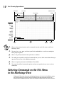
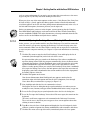
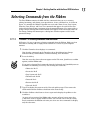
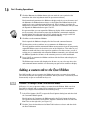
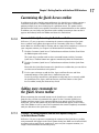
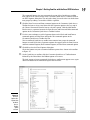
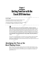
Chapter 1
AL
Getting Familiar with the
Excel 2010 Interface
▶ Selecting commands in the Excel Backstage View
TE
▶ Identifying the different parts of the Excel display screen
RI
In This Chapter
▶ Selecting commands on the Ribbon and Quick Access toolbar
MA
▶ Customizing the Ribbon and Quick Access toolbar
T
RI
GH
TE
D
he Excel 2010 interface relies primarily on the Ribbon, a block of commands
displayed at the top of the screen and divided into distinct blocks called tabs. The
single vestige of the old pull-down menus from versions prior to Excel 2007 is the File
menu that’s displayed along the left side of the brand new Backstage View screen. The
File menu contains all the File commands. You open the Backstage View that contains
the menu by clicking the File menu (which looks just like the Ribbon tabs in the worksheet
view except that it’s the only one that’s green). Also, in place of the many toolbars in
the pre-Excel-2007 versions, Excel 2010 offers a single toolbar called the Quick Access
toolbar.
CO
PY
The exercises in this first chapter are designed to get you familiar with the Excel 2010
interface. As a result of doing these exercises, you should be comfortable with all
aspects of the display screen and the command structure and ready to do all the rest of
the exercises in this book.
Identifying the Parts of the
Excel Display Screen
Before you can start using Excel 2010, you have to be familiar with its display screen.
Figure 1-1 shows you the Excel 2010 display screen as it first appears when you launch
the program. Note the names of the different parts of the display screen before you
perform Exercise 1-1.
10
Part I: Creating Spreadsheets
Name box
File menu
Worksheet area
Quick Access toolbar
Ribbon
Formula bar
Figure 1-1:
The Excel
2010
program
window
as it
appears
immediately after
launching
the
program.
Sheet
tabs
Status
bar
View
buttons
Zoom
control
Q.
What are the primary functions of the commands located on the File menu in the Excel
Backstage View?
A.
To open, close, save, print, and share your Excel workbook files as well as to modify the
Excel program options.
Q.
What is the primary function of the Quick Access toolbar?
A.
To enable you to quickly select Excel commands that you use all the time without having to
open the File menu or use the Ribbon commands.
Q.
What’s the primary function of the Ribbon in Excel 2010?
A.
To group related Excel commands together and give you quick and easy access to these
commands.
Selecting Commands on the File Menu
in the Backstage View
Clicking the File menu, the green tab-looking thingy at the far left of the Ribbon, opens
the Excel Backstage View with a menu of options that appears down the left side.
Almost all the commands on this menu are related to actions that affect the entire file,
Chapter 1: Getting Familiar with the Excel 2010 Interface
such as saving and printing. If you prefer, you can open this view and access the menu
by pressing Alt+F (F for File) instead of clicking the File menu.
When you select any of the major options on this menu — Info, Recent, New, Print, Save
& Send, or Help — panels appear that bring together further related and commonly
used menu options on the left side along with pertinent information and, in the case, of
the Info and Print options, document previews, on the right side.
Before you attempt the exercises in this chapter, you may want to play the Using the
Excel 2010 Ribbon and Backstage.exe demo located in the Excel Feature Demo folder
on your workbook CD-ROM. This video demonstrates selecting commands from the File
menu as well as on the Ribbon and Quick Access toolbar.
Exercise 1-1: Opening the Backstage View and Selecting Its Menu Commands
In this exercise, you get familiar with the new Excel Backstage View and the commands
on its File menu as you practice opening the Backstage View and selecting some of its
menu commands. Make sure that Excel 2010 is running and an empty Sheet1 worksheet
is active on your computer monitor (see Chapter 2 if you need information on launching
Excel).
1. Click the File menu to switch to the Excel Backstage View and display the list of
commands (Info through Exit) on the left side of this screen.
Keep in mind that when you switch to the Backstage View when no workbook is
open for editing in Excel 2010, the program automatically selects the Recent menu
command that displays a Recent Workbooks pane on the left with a list of recently
opened workbook files and a Recent Places pane on the right with a list of file
folders recently opened. When you switch to the Backstage View when a workbook
file is open for editing, Excel selects the Info option at the top of the menu instead,
displaying a panel with a thumbnail of the current worksheet and a list of properties
describing aspects of the file.
2. Click the Info option on the menu.
Note that an Information about Book1 panel now appears attached to the
immediate right of the Info option and that all of the suboptions, Save through
Close above Info, are indented as a group (see Figure 1-2).
3. Now, highlight and click the Save As command to select it.
Excel opens the Save As dialog box in the regular worksheet view where you can
modify the name, location, and type of Excel workbook file before saving a copy of it.
4. Press the Esc (Escape) key on your keyboard to close the Save As dialog box.
5. Press Alt+F to open the Backstage View with its File menu again, this time from the
keyboard.
This time, small letters appear on each command in the Backstage View menu.
These are the access keys that you can type to select a menu option rather than
clicking its name or button.
6. Type D to select the Save & Send option and display the Save & Send panel, which
contains a number of options for sharing workbook files with coworkers and clients.
7. Click the File menu at the top of the menu, immediately above the Save option.
11
12
Part I: Creating Spreadsheets
8. Press Ctrl+P (the shortcut key for printing in Excel).
Excel selects the Print command on the menu in the Backstage View and displays
a Print panel where you can preview the printout (when there’s data in your
worksheet that can be printed) and change simple print settings. Because you
selected the Print panel from an empty worksheet, the message, “Microsoft Excel
did not find anything to print” appears on the right panel where the first page of
the workbook’s print preview normally appears.
9. Press the Escape key to return to the normal worksheet view and then press
Alt+FT.
Doing this selects the Options command in the Backstage View, which in turn,
opens the Excel Options dialog box in the regular worksheet view. This dialog box
contains all the options for changing the Excel program and worksheet options.
These options are divided into categories General through Trust Center.
10. Click the Advanced button in the left pane to display all the Advanced options in
the right pane. Next, scroll down to the Display Options for This Worksheet section
and click the Show Page Breaks check box to remove its check mark before you
click the OK command button to close the dialog box.
Note that deselecting the Show Page Breaks option in the Excel Options dialog box
removes all the dashed page break lines from the Sheet1 worksheet.
Figure 1-2:
The Excel
Backstage
View when
the Info
menu option
is selected.
Chapter 1: Getting Familiar with the Excel 2010 Interface
Selecting Commands from the Ribbon
The Excel Ribbon contains the bulk of all the commands that you use in creating,
editing, formatting, and sharing your spreadsheets, charts, and data lists. As shown in
Figure 1-2, normally the Ribbon is divided into seven tabs: Home, Insert, Page Layout,
Formulas, Data, Review, and View. The commands that appear on each tab are then
further divided into Groups, containing related command buttons. Also, many of these
groups contain a Dialog Box Launcher button that appears in the lower-right corner of
the Group. Clicking this button opens a dialog box of further options related to the
particular Group.
Exercise 1-2: Selecting Commands from the Ribbon
In Exercise 1-2, you get practice selecting commands from the Ribbon. Make sure that
Excel 2010 is running and an empty Sheet1 worksheet is active on your computer
monitor.
1. Click the Formulas tab to displays its commands.
Note that the commands on the Formulas tab are divided into four Groups:
Function Library, Defined Names, Formula Auditing, and Calculation.
2. Press the Alt key.
Note the access-key letters that now appear on the File menu, Quick Access toolbar
options, and the Ribbon tabs.
If you prefer selecting Excel commands from the keyboard, you’ll probably want to
memorize the following access keys for selecting the seven tabs:
• Home tab: Alt+H
• Insert tab: Alt+N
• Page Layout tab: Alt+P
• Formulas tab: Alt+M
• Data tab: Alt+A
• Review tab: Alt+R
• View tab: Alt+W
3. Type W to display the contents of the View tab and then type VG to remove the
check mark from the Gridlines check box in the Show Group.
4. Click the Gridlines check box to select it again and redisplay the gridlines in the
worksheet.
As you may have noticed, the Ribbon takes up quite of bit of screen space that
is otherwise used to display worksheet data. You can take care of this by setting
Excel to minimize the Ribbon each time you select one of its commands to display
only the tab names.
13
14
Part I: Creating Spreadsheets
5. Click the Minimize the Ribbon button (the one with the caret symbol to the
immediate left of the help button with the question mark icon).
Excel immediately minimizes the Ribbon to display only the seven tab names and
the Minimize the Ribbon button changes to the Expand the Ribbon button (indicated by the caret symbol pointing downward). Excel continues to reduce the
Ribbon to its tab names any time after you select one its commands until you click
the Expand the Ribbon button or press Ctrl+F1.
Keep in mind that you can expand the Ribbon to display all the command buttons
on the currently selected tab any time that the Ribbon is minimized simply by
double-clicking the tab or pressing Ctrl+F1 (which acts like a toggle switch for
altering between a minimized and fully maximized Ribbon).
6. Click Data on the minimized Ribbon.
Excel expands the Ribbon to display all of the Data tab command buttons.
7. Click anywhere in the worksheet area to minimize the Ribbon once again.
The only problem with this minimized Ribbon arrangement is that the temporarily
expanded Ribbon covers the first three rows of the worksheet. This makes it very
difficult to work with data at the top of the worksheet. For that reason, as well as
to help you get comfortable with unfamiliar Ribbon commands, you will work with
the Ribbon expanded at all times in all remaining exercises in this workbook.
8. Press Ctrl+F1 to maximize the Ribbon and then click the Home tab to displays its
command buttons.
The Ribbon now remains fully displayed at all times as you select any of its tabs
and command buttons without ever obscuring any part of the worksheet display.
Adding a custom tab to the Excel Ribbon
Excel 2010 enables you to customize the Ribbon by creating a custom tab to which
you can then add your own groups of commands. When you create a custom tab, Excel
automatically assigns an available hot key to it.
Exercise 1-3: Adding a Custom Tab to the Excel Ribbon
In Exercise 1-3, you get practice adding a custom tab to the Ribbon. Make sure that
Excel 2010 is running and an empty Sheet1 worksheet is active on your computer
monitor (see Chapter 2 for information on launching Excel).
1. Select File➪Options (Alt+FT) to open the Excel Options dialog box and then click
the Customize Ribbon option.
Excel displays the Customize the Ribbon panel in the Excel Options dialog box.
This panel is divided into two list boxes: Popular Commands on the left side and
Main Tabs on the right side (see Figure 1-3).
2. Click the View tab check box in the Main Tabs list box to select it and then click
the New Tab button.
Chapter 1: Getting Familiar with the Excel 2010 Interface
Excel inserts a generic New Tab (Custom) with a generic New Group (Custom)
right below it. This custom tab and group appear between the View tab and the
Developer tab in the Main Tabs list box.
3. Click New Tab (Custom) in the Main Tabs list box to select it and then click the
Rename command button.
Excel opens the Rename dialog box where you can replace the generic New Tab
display name with a descriptive name.
4. Replace New Tab by typing Misc (for Miscellaneous) in the Display Name text box
and then select OK.
Misc (Custom) now appears in the Main Tabs list box sandwiched between View
and Developer.
Figure 1-3:
The Excel
Options
dialog box
with the
Customize
Ribbon
option
selected.
Adding commands to groups on your custom tab
After you add a custom tab to the Excel 2010 Ribbon, you can then start adding the
commands you want to appear on this tab. Just as with the standard Ribbon tabs,
the commands you add on your own custom tab are arranged in groups. When you first
create a custom tab, it contains only a single, generic New Group (Custom) into which
to add your commands. You can, however, add other groups to the custom tab using
the New Group command button as well as give these groups their own descriptive
names using the Rename command button.
15
16
Part I: Creating Spreadsheets
Exercise 1-4: Adding Commands to a Custom Tab
In Exercise 1-4, you get practice adding commands to the custom tab you added to the
Ribbon in Exercise 1-3. Before you start this exercise, make sure that the Excel Options
dialog box is still open with a Misc (Custom) tab appearing in the Main Tabs list box
between View and Developer.
1. Click the New Group (Custom) listing under Misc (Custom) in the Main Tabs list
box to select it and then click the Rename button.
Excel opens the Rename dialog box where you can replace the generic New Group
name with your own descriptive name.
2. Replace New Group by typing Data Form in Display Name text box and then
selecting OK.
Data Form (Custom) now appears as the sole group on the Misc custom tab in the
Main Tabs list box. Now, you’re ready to add the Form command button to the
Data Form group that you can use later on when completing some of the exercises
in Chapter 17.
3. Click the drop-down button to the right of Popular Commands in the Choose
Commands From drop-down list box at the top of the left side of the Customize the
Ribbon panel and then click Commands Not in the Ribbon.
Excel now displays an alphabetical list of commands that are not currently on the
Ribbon in the list box on the left.
4. Click the Form button in this Commands Not in the Ribbon list box and then click
the Add command button.
Excel adds the Form button under the Data Form (Custom) group in the Main Tabs
list box.
5. Click the OK button to close the Excel Options dialog box.
The custom Misc tab you just created now appears at the end of the Excel 2010
Ribbon.
6. Click the Misc tab or press Alt+Y to select this tab.
The Misc tab is selected, displaying its sole Form button in the single Data Form
group.
7. Click the Home tab to select it.
Selecting Commands on the
Quick Access Toolbar
When you first start working with Excel 2010, the Quick Access toolbar contains only
the following three simple command buttons:
✓ Save to save changes to your current workbook file
✓ Undo to reverse the effect of the last change you made to a worksheet
✓ Redo to restore the last change you reversed with the Undo button
Chapter 1: Getting Familiar with the Excel 2010 Interface
Customizing the Quick Access toolbar
In addition to the three default command buttons, the Quick Access toolbar contains a
Customize Quick Access Toolbar button (the one with the line above a downward
pointing triangle) that, when clicked, opens a pull-down menu. The options on this
pull-down menu enable you to quickly customize the command buttons on this toolbar.
In addition, you can change the placement of the toolbar by moving it down so that it
appears immediately below the Ribbon and above the Formula bar.
Exercise 1-5: Quickly Customizing the Quick Access Toolbar
In Exercise 1-5, you get practice customizing the contents and position of the Quick
Access toolbar using options that appear on the Customize Quick Access Toolbar
menu. Make sure that Excel 2010 is running and an empty Sheet1 worksheet is active on
your computer monitor (see Chapter 2 for information on launching Excel).
1. Click the Customize Quick Access Toolbar button and then click the Show Below
the Ribbon option on its menu.
The Quick Access toolbar with its three command buttons and the Customize
Quick Access Toolbar button now appears immediately above the Formula bar.
2. Click the Customize Quick Access Toolbar button and then click the Quick Print
option.
Excel adds the Quick Print button to the Quick Access toolbar that you can click to
send the current worksheet to the printer.
3. Use the same technique to add the New, Open, and Print Preview and Print
command buttons to the Quick Access toolbar on your own.
Use the ScreenTips attached to each button to verify that you’ve correctly added
the Quick Print, New, Open, and Print Preview and Print buttons to the Quick
Access toolbar, noting the shortcut keys listed.
Adding more commands to
the Quick Access toolbar
When customizing the command buttons on the Quick Access toolbar, you aren’t
limited to the selection of commands that appear on the Customize Quick Access
Toolbar pull-down menu. Using command options that appear in the Excel Options
dialog box, you can add buttons for any of the commands that appear on the various
tabs of the Ribbon as well as some Excel commands that remain completely unavailable
until you add them to the Quick Access toolbar.
Exercise 1-6: Adding Commands from the Excel Options Dialog Box
to the Quick Access Toolbar
In Exercise 1-6, you get practice customizing the contents of the Quick Access toolbar
using commands that appear in the Excel Options dialog box. Make sure that Excel 2010
is running and an empty Sheet1 worksheet is active on your computer monitor (see
Chapter 2 for information on launching Excel).
17
18
Part I: Creating Spreadsheets
1. Click the Customize Quick Access Toolbar button and then click the More
Commands option on its menu.
Excel opens the Excel Options dialog box with the Quick Access Toolbar tab
selected (see Figure 1-4). This dialog box contains two list boxes:
• The Choose Commands From list box on the left where you select the
commands to add to the toolbar
• The Customize Quick Access Toolbar list box on the right, showing the
buttons on the toolbar and their order
To add a new command to the toolbar, you select it in the Choose Commands
From list box and then click the Add button. To reorder the buttons on the toolbar,
you click its command button in the Customize Quick Access Toolbar list box and
then click the Move Up or Move Down buttons (with the black triangles pointing
up and down, respectively) until the selected button is in the desired position.
2. Click the drop-down button on the Choose Commands From drop-down list box
and then click the Commands Not in the Ribbon option on its drop-down menu.
The Choose Command From list box now contains only command buttons that are
not found on the various tabs of the Excel Ribbon.
3. Click the AutoFormat command option in the Choose Commands From list box
(the one with the lightning bolt on top of a small table) and then click the Add
button.
The AutoFormat command option is now listed at the very bottom of your
Customize Quick Access Toolbar list box, indicating that it is now the last button
on the Quick Access toolbar.
4. On your own, add the Calculator, Draw Borders, Speak Cells, Speak Cells – Stop
Speaking Cells, Speak Cells by Columns, Speak Cells by Rows, and Speak Cells on
Enter command options to the Quick Access toolbar.
You may have to scroll down the list of command options in the Choose
Commands From list box in order to select and add the Draw Borders, Form, and
the different Speak Cells command options to the Quick Access toolbar.
Next, you want to modify the order in which the command buttons appear on your
customized Quick Access toolbar so that they appear in this order arranged in four
groups:
• New, Open, Save, Quick Print, and then Print Preview and Print
• Undo and then Redo
• AutoFormat, Calculator, and Draw Borders
• Speak Cells, Speak Cells – Stop Speaking Cells, Speak Cells by Columns, Speak
Cells by Rows, and Speak Cells on Enter
5. Click the New command option in the Customize Quick Access Toolbar list box
to select it and then click the Move Up button (the one with the black triangle
pointing upward) until New is the first command in this list (four times).
6. Use the same technique to move the Open command button up until it appears
between the New and the Save button.
7. Use the Move Down button to move the Undo and Redo buttons so that they now
appear in the same order below the Quick Print and Print Preview and Print buttons.
Chapter 1: Getting Familiar with the Excel 2010 Interface
The command buttons for your customized version of the Quick Access toolbar
now appear in the correct order in the Customize Quick Access Toolbar list box in
the Excel Options dialog box. The only other thing you need to do is to divide them
into groups by adding a vertical bar called a separator.
8. Click the Print Preview and Print command option in the Customize Quick Access
Toolbar list box to select it and then click the Separator option at the very top of
the Choose Commands From list box to select this option. Click the Add button.
Excel inserts a separator between the Print Preview and Print and Undo command
options in the Customize Quick Access Toolbar list box.
9. Use this same technique to add a Separator between the Redo and AutoFormat
command options and the Form and Speak Cells command options in the
Customize Quick Access Toolbar list box.
Your customized Quick Access toolbar now contains four groups of command
buttons created by the three Separator options that appear after the Print Preview
and Print command option, Redo command option, and the Form command option.
10. Click OK to close the Excel Options dialog box.
Check the buttons on your customized toolbar against those shown in the toolbar
in Figure 1-5.
11. On the Quick Access toolbar, click the Customize Quick Access Toolbar button
followed by the Show Above the Ribbon option on its menu.
The final version of your customized Quick Access toolbar now appears once again
above the Ribbon to the immediate right of the File menu.
Figure 1-4:
The Excel
Options dialog box with
the Quick
Access
Toolbar
option
selected.
19
20
Part I: Creating Spreadsheets
Calculator Speak Cells by Column
Print Preview and Print
New Save
Redo
Speak
Speak Cells
Cells by Rows
Figure 1-5:
The top part
of the Excel
display
screen with
the custom
Misc tab
and the
customized
Quick
Access
Toolbar.
Open
Undo
Quick Print
Draw
Borders
Auto Format
Speak
Cells
on
Enter
Speak Cells – Stop Speaking