Download Wiley Excel 2007 For Dummies Quick Reference

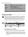
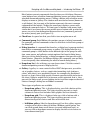
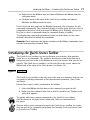
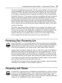
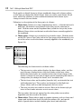
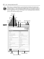
Part 1
AL
Getting to Know
Excel 2007
CO
PY
RI
GH
TE
D
MA
TE
RI
With Microsoft’s popular Excel 2007 spreadsheet program, you can enter, manipulate, and analyze data in ways that would be impossible, cumbersome, or error
prone for you to do manually. This part gives you the basics you need to get up
and running quickly in Excel.
In this part . . .
Familiarizing Yourself with the Excel 2007 Window
Navigating with the Mouse and Keyboard
Introducing the Ribbon, Quick Access Toolbar, and Office Menu
Formatting with Themes and Previewing Your Formatting Live
2
Part 1: Getting to Know Excel 2007
Excel Basics
Excel documents are known as workbooks. A single workbook can store as many
sheets as will fit into memory, and these sheets are stacked like the pages in a
notebook. Sheets can be either worksheets (a normal spreadsheet-type sheet with
rows and columns) or chart sheets (a special sheet that holds a single chart).
Most of the time, you perform tasks in worksheets. In older versions of Excel
(well, except for really old versions), each worksheet used a grid with 65,536
rows and 256 columns. Excel numbers rows starting with 1 and assigns letters to
columns starting with A. After Excel exhausts the letters of the alphabet, column
lettering continues with AA, AB, and so on. So column 1 is A, column 26 is Z,
column 27 is AA, column 52 is AZ, column 53 is BA, and so on. Prior to Excel
2007, row numbers ranged from 1 to 65,536 and column labels ranged from A
(column 1) to IV (column 256).
Excel 2007 increases the number of rows and columns in a single worksheet significantly. A worksheet now has 1,048,576 rows (no, that’s not a typo) and 16,384
columns (no, that’s not a typo either). Rows are numbered from 1 to 1048576
and columns are labeled from A to XFD.
The intersection of a row and a column is called a cell. A quick calculation using
Excel tells me that this works out to 17,179,869,184 cells — more than enough
for just about any use. Cells have addresses, which are based on their row and
column. The upper-left cell in a worksheet is called A1, and the cell down at
the bottom right is called XFD1048576. Cell K9 (also known as the dog cell) is the
intersection of the eleventh column and the ninth row.
You might be wondering about the amount of system memory (known as random
access memory, or RAM) you need to accommodate all those rows and columns.
The actual memory you need depends on the amount of data you store in the
workbook and the number of open workbooks. The good news is that Excel 2007
allows you to work with more memory than previous versions. Excel 2003, for
example, will utilize up to only 1 GB (gigabyte) of memory, even if your system has
more memory available. In Excel 2007, the memory available is limited by the maximum amount of memory that your version of Windows (XP or Vista) can use.
Formulas
A cell in Excel can hold a number, some text, a formula, or nothing at all. You
already know what numbers and text are, but you may be a bit fuzzy on the concept of a formula. A formula tells Excel to perform a calculation using information stored in other cells. For example, you can insert a formula that tells Excel
to add the values in the first 10 cells in column A and to display the result in the
cell that contains the formula.
Excel Basics — Familiarizing Yourself with the Excel 2007 Window
3
Formulas can use normal arithmetic operators such as + (plus), — (minus),
* (multiply), and / (divide). They can also use special built-in functions that
let you do powerful things without much effort on your part. For example,
Excel has functions that add a range of values, calculate square roots, compute
loan payments, and even tell you the time of day. Part 5 covers how to use the
various functions in Excel.
Active cell and ranges
In Excel, one of the cells in a worksheet is always the active cell. The active cell
is the one that’s selected, and it’s displayed with a thicker border than the
others. Its contents appear in the formula bar. You can select a group, or range,
of cells by clicking and dragging the mouse pointer over them. You can then
issue a command that does something to the active cell or to the range.
The selected range is usually a group of contiguous cells, but it doesn’t have to
be. To select a noncontiguous group of cells, select the first cell or group of
cells, hold down the Ctrl key while you drag the mouse, and select the next cell
or group of cells.
Familiarizing Yourself with the Excel 2007 Window
Figure 1-1 shows a typical Excel 2007 window, with the important parts labeled.
This terminology rears its ugly head throughout the book, so look at the figure
carefully.
Moving, resizing, and closing windows
When Excel and workbook windows are in a restored state (between a maximized
and minimized state, that is) you can use the resize handles to adjust the window
size to your liking. Move the mouse pointer to the area of the resize handle until
the pointer changes to a double-headed arrow, and then drag with the mouse.
You can move the window around the screen by dragging the title bars. See also
“Using the Mouse and Keyboard,” later in this part.
When the active workbook window is maximized, it shares a single Close button
with the Excel window. After you click the shared Close button, Excel closes the
active workbook.
Exiting Excel
Use any one of the following methods to close the Excel application:
Click the Close button on the Excel title bar if one or no workbook is open.
Click the Office button and then click the Exit Excel button.
4
Part 1: Getting to Know Excel 2007
Double-click the Office button. See “Introducing the Office Menu,” later in
this part.
Press the Alt key, then press F, and then press X.
Select all button
Control button
Mouse pointer
Office button
Split box
Formula bar
Name box
Excel title bar
Quick Access toolbar
Active
cell
pointer
Help
Close
Workbook title bar
Column
header
Maximize/Restore
Workbook window
Minimize
Figure 1-1
Sheet tabs
Row header
Status bar
New sheet tab
Tab scrolling controls
Tab split
Zoom controls
Scroll bar
Split box
Normal view Page break preview
Page layout view
Window resize handles
Familiarizing Yourself with the Excel 2007 Window — Navigating with the Mouse and Keyboard
5
Navigating with the Mouse and Keyboard
The mouse is the primary tool that you use in Excel for executing commands,
making selections, and navigating in the worksheet. Following are the mouse
conventions that we use in this book:
Click: Click the left mouse button once.
Double-click: Click the left mouse button twice in quick succession. It may
take you some time to get the hang of this action.
Right-click: Click the right mouse button once.
Drag: Hold down the left mouse button and move the mouse. Release the
mouse button to complete the drag operation.
Hover: Place the mouse pointer over an element without clicking a mouse
button.
Select: Place the mouse pointer over an element and click the left mouse
button.
Mousing around
Every mouse action is associated with some element in the Excel window. An
element can be a slider, button, cell, chart object, and so on. You select or hover
over the element using the mouse pointer.
Navigating through a worksheet with a mouse works just as you’d expect. Just
click a cell, and it becomes the active cell. If the cell that you want to activate
isn’t visible in the workbook window, you can use the scroll bars to scroll the
window in any direction, as follows:
To scroll one cell, click one of the arrows on the scroll bar.
To scroll by a complete screen, click either side of the scroll bar’s slider
button (the large center button).
To scroll faster, drag the slider.
To scroll a long distance vertically, press and hold the Shift key while drag-
ging the slider button.
Note that only the active workbook window displays scroll bars. If you activate a
different window, its scroll bars appear.
After you right-click a cell, a range of cells, or another object in the worksheet
area, Excel displays a contextual menu, so-called because the menu includes
commands specific to working with the cell, range, or object.
6
Part 1: Getting to Know Excel 2007
For your convenience, Excel 2007 adds a mini-toolbar above the contextual
menu with useful commands drawn from the Ribbon, as shown in Figure 1-2. See
also “Introducing the Ribbon,” later in this part.
Figure 1-2
Using the keyboard
Most users will be comfortable using the mouse to do all their work in Excel. For
users who prefer to use the keyboard exclusively when working in Windows
applications or for users who prefer to split the use of the mouse and keyboard
among various tasks, Excel provides the following solutions.
Keyboard shortcuts
Keyboard navigation
KeyTips
The first two functions are described next. For more on the last function,
KeyTips, see “Tipping off your keyboard,” later in this part.
You can access commands in Excel using keyboard shortcuts, which are individual keystrokes or a combination of keys pressed simultaneously. To access the
Print command using a shortcut, for example, you press and hold down the Ctrl
key and press the P key, represented in this book as Ctrl+P. The following table
lists some common keyboard shortcuts in Excel.
Shortcut
Action
Ctrl+A
Select all
Ctrl+B
Apply or remove bold formatting
Ctrl+C
Copy selection
Navigating with the Mouse and Keyboard
Shortcut
Action
Ctrl+F
Find
Ctrl+G or F5
Go To
Ctrl+H
Replace
Ctrl+I
Apply or remove italic formatting
Ctrl+O or Ctrl+F12
Open a document
Ctrl+P
Print
Ctrl+S or Shift+F12
Save
Ctrl+U
Apply or remove underlining
Ctrl+V
Paste
Ctrl+W or Ctrl+F4
Close the active workbook
Crtl+X
Cut
Ctrl+Y or F4
Repeat the last action
Ctrl+Z
Undo the last action
F1
Display the help viewer
Ctrl+F1
Hide or display the Ribbon commands
F2
Enable editing within the active cell
7
With more than 17 billion cells in a worksheet, you need ways to move to specific cells. Fortunately, Excel provides you with many techniques to move
around a worksheet. As always, you can use either your mouse or the keyboard
on your navigational journeys. The following table lists the keystrokes that
enable you to move through a worksheet.
Keys
Action
Up arrow
Moves the active cell one row up
Down arrow
Moves the active cell one row down
Left arrow
Moves the active cell one column to the left
Right arrow
Moves the active cell one column to the right
PgUp
Moves the active cell one screen up
PgDn
Moves the active cell one screen down
Alt+PgDn
Moves the active cell one screen right
Alt+PgUp
Moves the active cell one screen left
Home
Moves the active cell to the first column of the row that the active cell
is currently in
cont.
8
Part 1: Getting to Know Excel 2007
Keys
Action
Ctrl+Home
Moves the active cell to the beginning of worksheet (A1)
F5
Displays the Go To dialog box
Ctrl+Backspace
Scrolls the screen to display the active cell
Up arrow*
Scrolls the screen one row up (active cell doesn’t change)
Down arrow*
Scrolls the screen one row down (active cell doesn’t change)
Left arrow*
Scrolls the screen one column left (active cell doesn’t change)
Right arrow*
Scrolls the screen one column right (active cell doesn’t change)
* With Scroll Lock on
Introducing the Ribbon
Excel 2007 comes with a new user interface that replaces the standard menus
and toolbars found at the top of the window in previous versions of Excel. The
new interface is called the Ribbon and consists of a series of tabs, each containing a variety of commands grouped according to function (see Figure 1-3).
Virtually all the features in Excel 2007 are available through the commands in
the Ribbon tabs. This arrangement allows you to discover features in the program far more easily than if you had to drill down several layers into menus.
Home tab
Contextual tab header
Figure 1-3
Split button
Dialog launcher
Contextual tabs
Dissecting the parts of the Ribbon
The commands in the Ribbon are accessed through a variety of controls. Here’s a
list of the various types of controls and other parts that make up the Ribbon:
Button: This is the most common type of control. Most buttons in the
Ribbon (except the formatting ones) have descriptive text associated with
them, so you don’t need to be a Mensa expert to figure out what a button
represents. The most frequently used commands in each Ribbon tab have
larger buttons.
Navigating with the Mouse and Keyboard — Introducing the Ribbon
9
Most buttons execute commands directly when you click them. However,
some buttons have a built-in downward-pointing arrow, and others have an
attached downward-pointing arrow. Clicking a button with a built-in arrow
displays a menu or gallery. For a button with an attached arrow (known as
a split button), the icon part of the button represents the most common
command for the button. Clicking the arrow part displays a menu with
additional command choices. The two types of buttons with arrows look
similar but if you hover the mouse pointer over a button with an attached
arrow, you see a clear delineation between the icon (command) part and
the arrow (menu) part (see Figure 1-3).
Check box: A square box that you click to turn an option on or off.
Command group: Each Ribbon tab contains groups of related commands.
For example, you find commands related to text fonts in the Fonts group of
the Home tab.
Dialog launcher: A command that launches a dialog box (a pop-up window)
from within a command group, menu, or gallery. The dialog launcher in a
command group is a little button in the bottom right of the group. In addition, some menus and galleries contain options that launch dialog boxes.
After you click a dialog launcher, a dialog box appears that presents additional choices. (However, the Ribbon displays the commands you are likely
to use frequently, thus minimizing the need to launch dialog boxes.)
Drop-down list: A list of things you can choose from. Click the control’s
downward-pointing arrow to display the list.
Gallery: A gallery is a new control in Excel 2007 that presents you with a
set of graphic choices, such as a particular formatting style (patterns,
colors, and effects) or a predefined layout. An example of a predefined
layout is a chart choice with specific elements preselected for inclusion in
the chart. Galleries enable Excel to be more results oriented; that is, they
present the likely result you are looking for first and then expose advanced
choices through a dialog box or Ribbon command.
Three types of galleries are available:
• Drop-down gallery: This is displayed after you click a button with a
downward-pointing arrow. This type of gallery presents a single
column of choices and includes both graphic and text elements.
• Drop-down grid: This is displayed after you click a button with a
downward-pointing arrow. This type of gallery presents a twodimensional grid of choices and does not include text.
• In-Ribbon gallery: Like the drop-down grid, but this gallery exposes
a single row of choices directly within a Ribbon control group. You
can click up and down scroll arrows to reveal additional rows, or
you can click a drop-down arrow to display the full set of choices in
a two-dimensional grid.
10
Part 1: Getting to Know Excel 2007
Help button: On the far right of the Ribbon is the help button (the question
mark). Click this button for general Excel help.
Menu, rich: Rich menus are new in Excel 2007. Each menu choice has an
illustrative graphic, the command name, and in some cases a short
description of what the command does.
Don’t confuse rich menus with drop-down galleries, although they look
similar. Menus contain related commands. Galleries allow you to choose
from among a set of formats or layouts.
Menu, standard: Most users are already familiar with this form of menu —
a drop-down list of choices with command names (such as Paste or Insert
Cells). Some command names have small associated icons. If you click a
command name that ends with an ellipsis (...), Excel displays a dialog box
that presents further choices.
Spinner: A control with two arrows (one pointing up, the other pointing
down) used with an input box to specify a number (height or width, for
example.) Clicking an arrow increases or decreases the number in the
input box. You can also enter a number in the box directly. The spinner
control allows you to use only valid numbers.
Tab, contextual: Contextual tabs give the Ribbon the power to expose all
features in Excel. One or more contextual tabs appear after you insert or
select an object, such as a chart, shape, table, or picture. For example,
after you insert a chart, three contextual tabs related to chart functionality
appear on the Ribbon and a header labeled Chart Tools appears on the
Excel title bar above the contextual tabs. Contextual tabs contain all the
commands you need for working with the particular object. After you
deselect an object, the contextual tabs (and the header) disappear.
The general rules that govern the display of contextual tabs follow:
• After you select an object (such as a chart, shape, or table), one or
more contextual tabs for the object appear on the Ribbon. You must
select a tab to display the associated commands.
• After you insert an object, Excel displays the commands for the first
tab of the contextual tab set for that object.
• After you double-click an object, Excel displays the commands for the
first tab of the contextual tab set for that object. Note that not all
objects have this double-click capability.
• After you select, deselect, and then reselect the object without using
any other commands in-between, Excel displays the commands for the
first tab of the contextual tab set for that object.
Introducing the Ribbon
11
Tab, standard: The Ribbon comes with a set of standard tabs, each
organized according to the functions of the commands that it contains.
For example, the Insert tab contains command groups to insert shapes,
charts, tables, pictures, and so on. An exception is the Home tab, which
is so-named because this is where you do most of your work in Excel.
If your mouse has a scroll wheel, you can navigate quickly among the
Ribbon tabs by hovering the mouse pointer over the Ribbon area and
scrolling the wheel back and forth.
Text box: A box in which you enter a number or text. In general, the Ribbon
associates a text box with another control, such as a spinner or a dropdown box.
Sizing up the Ribbon
The layout of the Ribbon controls is not static. Depending on your screen resolution, or the Excel window size, or both, the Ribbon provides one of four layout
options for command groups. If sufficient space is available, the Ribbon presents
a layout that labels commands, displays more commands individually, and eliminates extra clicks. As you resize the Ribbon downwards (by reducing the screen
resolution or shrinking the size of the Excel window), the Ribbon rearranges the
layout of some of the command groups by first resizing command buttons (larger
buttons become smaller), then removing labels from commands, and finally reducing the groups to single large buttons (see Figure 1-4). To access the commands in
a command group that the Ribbon resizes to a single button, you must first click
the button to display a flyout menu and then select the command.
Figure 1-4
It is important to note that at each stage of downward resizing, no command
groups or commands disappear entirely from the Ribbon. The multiple layout
options for the command groups ensure that nothing is lost as space becomes
more limited. If you reduce the size of the Excel window sufficiently, however,
the Ribbon disappears altogether.
12
Part 1: Getting to Know Excel 2007
Tipping off your keyboard
Excel provides a feature called KeyTips that allow you to access every command
on the Ribbon using the keyboard, without having to memorize keystroke combinations! So, what are KeyTips? KeyTips are little alphanumerical indicators
containing a single letter, a combination of two letters, or a number, indicating
what to type to activate the command under them, as shown in Figure 1-5.
Figure 1-5
Follow these steps to access a command in a Ribbon tab using a KeyTip:
1. Press the Alt key. The KeyTips appear over the Ribbon tabs (Ignore the
KeyTips that appear in the other areas of the interface for this exercise.)
2. Press the key that represents the KeyTip for the Ribbon tab you want to
access. For example, press N to select the Insert tab. Note that you do not
have to hold down the Alt key. If you need to select a different tab after
you select the KeyTip for a tab, press the Esc key.
3. Press the key or key combination that represents the KeyTip for the com-
mand you want to use.
If the command you select is a drop-down gallery or drop-down grid, you can
use an arrow key or the Tab key to highlight your choice and then press the
Enter key to select your choice.
Remember: KeyTips are associated with in-Ribbon galleries, so you have to press
the key that represents the KeyTip for the gallery before you can choose an
option in the gallery.
Remember: If the command you want to use requires a number key, you must use
the number keys on the main keyboard. The KeyTip feature does not work with
the numeric keypad.
Hiding the Ribbon commands
If you find that the Ribbon commands take up too much of your screen area, you
can hide them using any of the following methods:
Press Ctrl+F1
Double-click any Ribbon tab
Introducing the Ribbon — Introducing the Quick Access Toolbar
13
Right-click in the Ribbon area and choose Minimize the Ribbon from the
contextual menu
Click the arrow to the right of the Quick Access toolbar and choose
Minimize the Ribbon from the menu
If you click a tab after you hide the Ribbon commands, Excel displays the tab
commands temporarily. The command display is hidden again after you select a
command in the tab or click away from the Ribbon area. Similarly, you can use
KeyTips to select a command when the command display is hidden.
To redisplay the commands permanently after you hide them, use the same
methods described for hiding the commands.
Remember: Excel maintains the hidden condition of the Ribbon commands if you
exit and subsequently re-launch Excel.
Introducing the Quick Access Toolbar
The Quick Access toolbar is an area of the new user interface that provides
quick access to commands. The toolbar is designed to reduce the amount of
navigation you have to do in the Ribbon to access the features that you use frequently. The Quick Access toolbar is on the left side of the screen, above the
Ribbon and to the right of the Office button (see Figure 1-6).
Figure 1-6
The Quick Access toolbar is the only area of the new user interface that you can
customize by adding commands to the three default commands (Save, Undo,
and Redo).
Follow these steps to add a command to the toolbar:
1. Select the Ribbon tab that houses the command you want to add.
2. Right-click the command and choose Add to Quick Access Toolbar in the
menu that appears.
To quickly add some common commands to the Quick Access toolbar,
click the arrow to the right of the toolbar and choose a command from
the menu.
You can add an entire command group to the Quick Access toolbar. Just rightclick an area in the command group name (for example, Font) and choose Add
to Quick Access Toolbar.
14
Part 1: Getting to Know Excel 2007
Follow these steps to remove a command (including the default commands)
from the toolbar:
1. Right-click the command you want to remove from the toolbar.
2. Choose Remove from Quick Access Toolbar in the menu that appears.
If you think you’ll be adding a lot of commands to the Quick Access toolbar, it’s a
good idea to move the toolbar from the title bar to a separate location below the
Ribbon. Right-click anywhere on the toolbar and choose Place Quick Access
Toolbar below the Ribbon in the menu that appears. You can regain screen area
for working in the worksheet by double-clicking a Ribbon tab (or pressing
Ctrl+F1) to hide the Ribbon controls temporarily.
You can access commands on the Quick Access toolbar using the keyboard. Press
the Alt key and then a number key that represents the KeyTip for the command
you want to access. See also “Tipping off your keyboard,” earlier in this part.
Introducing the Office Menu
Excel 2007 introduces a new menu for working with documents and accessing
special Excel options. The menu is accessed by clicking the Office button (the
large round button with the Office logo), located at the top-left corner of the
Excel screen. See Figure 1-7.
Figure 1-7
Introducing the Quick Access Toolbar — Formatting with Themes
15
The menu is divided into two sections. The left section contains a list of documentrelated commands. By default, the right section displays a list of recently used
documents. Click a document name in the list to open the file. Click a pushpin
to the right of a document name to keep the document on the list permanently.
By default, Excel lists 17 documents, which get overridden with new documents
unless you use the pushpin control. Some file commands on the left section
include a built-in or attached arrow. If you hover the mouse pointer over a command with an attached arrow, you will see a clear demarcation between the
button and the arrow. Clicking a button with a built-in arrow or the arrow portion of a button with an attached arrow displays additional choices in the right
section of the menu.
The Office menu also includes a button to access various Excel options and a
button to exit Excel. We encourage you to visit the options from time to time,
because you may find useful application, workbook, or worksheet options that
you want to turn on or off. An option in the Advanced section of the Excel
Options dialog box, for example, allows you to increase the number of documents displayed in the Recent Documents list to a maximum of 50.
Previewing Your Formatting Live
New in Excel 2007 is a Live Preview feature. When you hover over a formatting
option with the mouse pointer, Excel lets you see the effect that the formatting
option will have on your selection before you commit to applying the option.
Your selection might be a cell, range of cells, chart, table, shape, and more.
Suppose that you want to change the font of some text in a cell. In the Ribbon, a
drop-down box called the font picker presents a list of available fonts. As you
hover over each choice in the font picker, your cell updates to show you what
the text would look like if you chose that font. Live Preview avoids the normal
tedium of committing to an option, then undoing the option because the result
is not what you wanted, and then committing to another option, only to realize
that you don’t like the new result either, and so on.
You will find Live Preview options throughout Excel in places where formatting
alternatives are available — most notably in galleries.
Formatting with Themes
In Excel 2007, you can now use a formatting concept known as a theme. A theme
consists of a combination of fonts, colors, and effects that provide a consistent
look among your workbook’s elements, including cells, charts, tables, and
PivotTables. You apply the theme’s fonts, colors, and effects through individual
options or the style galleries of the various elements.
16
Part 1: Getting to Know Excel 2007
Excel applies a default theme to all new workbooks along with a theme gallery
so that you can change the default theme. After you select a new theme, all galleries and all the elements in your workbook formatted with theme styles
change to match the new theme.
Following is a description of the three parts of a theme:
Theme font: A theme uses two complementary fonts — a header font and a
body font. All elements using themed styles thus use the same font or
fonts. Click the arrow on the drop-down box (called the font picker) in the
Ribbon’s Home tab to see the fonts used in the theme currently applied to
the workbook.
Theme color: A theme uses a matched set of twelve colors. Click the arrow
on the Fill Color or Font Color tool in the Font group of the Home tab to see
ten of the colors used in the theme currently applied to the workbook (see
Figure 1-8).
Figure 1-8
The following are characteristics of theme colors:
• The top row in a color picker displays the base theme colors, and the
next five rows display various tints and shades of the base colors.
Below the theme colors are standard colors that do not change if the
theme is changed. If you want to apply specific formatting that doesn’t
change after you change the theme, use a standard color.
• The first four colors on the picker (from the left), are intended for text
and background use. These colors are designed so that light text
always shows well on a dark background, and vice versa.
• The next six colors are used for accents. Most of the theme-style galleries in Excel make extensive use of accent colors.
The two colors that are not exposed on the color pickers are used for
hyperlinks (not discussed in this book).
Theme effect: Theme effects apply to graphic elements such as charts and
shapes and include three levels of styles for outlines, fills, and special
effects. Special effects include shadow, glow, bevel, and reflection.
Formatting with Themes — Soliciting Help
17
You can change the theme in a workbook by clicking the Themes button in the
Ribbon’s Page Layout tab and selecting a new theme from the gallery that appears.
Remember: The three Microsoft Office applications — Excel 2007, Word 2007, and
PowerPoint 2007 — share the same themes. If you create reports that combine
elements from each application, your reports will have a consistent look if you
use a common theme.
Soliciting Help
With so many features and options available in Excel, it isn’t unusual to get
stuck once in a while. Fortunately, Excel provides the following methods for getting help easily:
Enhanced ScreenTips: Standard ScreenTips (also called ToolTips) have
been available in Excel for some time and provide textual context to
commands. After you hover your mouse pointer over a command in earlier
versions of Excel, Excel displays the action of the command using either a
single word (such as Paste) or a brief phrase (such as Increase Font Size).
A standard ScreenTip helps to decipher the meaning of a command button,
for example, when the button has no associated text and the command
meaning is unclear from the button icon.
Enhanced ScreenTips take the concept a step further by adding a short
description explaining the purpose of the command (hence the prefix
Enhanced). Some Enhanced ScreenTips include an explanatory graphic
when a text description is insufficient to explain the meaning of the command. Enhanced ScreenTips are available for all commands on the Ribbon.
In many cases, the ScreenTip explanation provides enough information, so
you don’t have to seek additional help. By default, Excel 2007 uses
Enhanced ScreenTips for all commands.
Contextual help: If the Enhanced ScreenTip doesn’t offer enough for you
to understand the use of a specific command, you can get more detailed
help. After you hover the mouse pointer over the command, the Enhanced
ScreenTip that pops up lets you know whether additional help for the command is available by indicating that you can press F1 for more help.
If you are in a dialog box and need help for the dialog box options, press
the help button (the question mark) to get contextual help.
General help: Click the help button (the question mark) on the right side
of the Ribbon or press F1 when you are not in a specific context (for example, the mouse pointer is not hovering over a command in the Ribbon) to
display a list of general help topics.
18
Part 1: Getting to Know Excel 2007
When you use contextual help or general help, Excel displays the help viewer,
shown in Figure 1-9. The viewer sports Internet browser-style controls. In fact, it
was built using the same technology that Microsoft uses in its Internet Explorer
browser application. Of course, the viewer is not a full-fledged browser because
you can view only Excel help content.
Search box
Home
Print
Refresh
Text size
Stop
TOC
Forward
Go (search)
Back
Pin
Maximize/Restore
Search scope Minimize
Figure 1-9
Status bar
Search result window
Connection status
Close
Soliciting Help
19
The major features of the help viewer follow:
Search box: You can enter specific search text in this box. The viewer
stores a list of your text searches for the current help session. Click the
drop-down arrow on the side of the box to view and select an item from the
list if you want to review a previous search result.
Search button: Click the Search button (or press Enter) to initiate a search
after you enter the search text in the search box. Click the arrow next to
the search button to define the search scope. By default, if your computer
is connected to the Internet, Excel will display help content from an online
source. If possible, you should use this source as your first choice because
Microsoft updates the contents of online help regularly.
If you are offline when you initiate a search, Excel uses help content internal to your system. You can force Excel to use internal help content always
by clicking the arrow next to the Search button and choosing Offline Excel
Help from the menu.
Whether online or offline, you can narrow you search scope further by
selecting an appropriate option from the Search button menu.
Search result window: This window displays the results of your search
request. If you use contextual help or enter text in the search box, the
window displays help information specific to the context of the search. If
you use general help, the window displays a list of general help topics in
the form of titled links. Clicking a link displays a new set of links with more
specific titles. Click the specific link title that best matches your search criterion to display detailed information on the topic.
Status bar: The left side of the status bar (located at the bottom of the help
viewer) displays the current search scope. The right side of the status bar
displays the connection status. You can click in the connection status area
to switch quickly between viewing online and offline help content.
Maximize/Restore button: Click this button for a full-screen view of the
help window. Click again to restore the window to its previous size.
Minimize button: Click this button to hide the help viewer window. Click
the Help button on the Windows taskbar (normally located below the Excel
window) to redisplay the viewer.
Close button: Click this button to close the help viewer.
Pin button: By default, Excel keeps the help viewer window on top when
you are working in the application. Use the Pin button to control this
behavior. If you “unpin” the viewer, Excel hides the window automatically if
you click anywhere inside the Excel window.
20
Part 1: Getting to Know Excel 2007
TOC (Table of Contents) button: Click this button to display a Table of
Contents pane on the left side of the help viewer. The pane displays the
same list of topics that the main windows displays after you select general
help or click the Home button. Clicking a main topic in the pane displays a
list of subtopics, similar to the subtopics that the main windows displays
after you click a general help topic link. The Table of Contents pane is convenient if you want to view the details of multiple subtopics in succession.
Text size button: Click this button to select a size for the text in the search
result window.
Print button: Click this button to print the help topic that the search result
window displays.
Home button: After browsing multiple helps topics in the search result
window, you might want to return to the list of main help topics to choose
another general topic link. Click the Home button to return to the list of
main help topics.
Refresh button: Click this button to refresh the help topic list after you
connect or disconnect from the Internet while the help viewer is open.
Stop button: Click this button to cancel a search request if the help viewer
is experiencing difficulties connecting to the online help source.
Back and Forward buttons: After browsing multiple helps topics in the
search result window, you might want to navigate among results and various
levels of detail. Click the Back or Forward button to perform your navigation.
If you want to resize the help viewer window, move the mouse pointer to any
edge of the window until the pointer changes to a double-headed arrow, and
then drag the mouse.