Download Agilent Technologies 54622D Specifications

An Introduction to Using the Agilent 54622D Digital Oscilloscope,
E3631A DC Power Supply, 34401A Digital Multimeter, and 33220A Arbitrary
Waveform Generator
By:
Walter Banzhaf
University of Hartford
Ward College of Technology
USA
Equipment Required
• Agilent 54622D Mixed-Signal Oscilloscope with two 10X attenuating probes and digital probe kit
• Agilent E3631A DC Power Supply
• Agilent 34401A Digital Multimeter with two test leads (one red, one black)
• Agilent 33220A Function/Arbitrary Waveform Generator
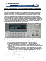
Introduction:
This is a basic introduction to four pieces of equipment listed above; be sure to consult the
Agilent manuals for each piece of equipment for information on safety, operational details,
specifications and other information.
Basic electronic laboratory equipment allows us to supply DC power to a circuit (using the DC
power supply, if the equipment doesn't have its own power supply), measure voltages, currents
and resistances in the circuit (with the digital multimeter), apply time-varying signals (e.g. sine
waves and square waves) to the circuit (with the function/arbitrary waveform generator), and
observe displays of voltage versus time (using the oscilloscope). The mixed-signal oscilloscope
allows us to look at analog signals and up to 16 digital signals simultaneously.
This experiment is based on the 90/10 philosophy: 90% of the time, one uses 10% of the
features of a product, be it a computer, software (such as a word processor), a car, or electronic
test and measurement equipment. After completing this experiment you will have a solid
understanding of how to make use of these four basic laboratory instruments.
1
Page
1
2
Procedure
Equipment Required, Introduction
Table of Contents
3
4
5
7
8
9
10
11
12
13
14
Part One – The Agilent 54622D Mixed-Signal Oscilloscope- Analog Inputs
Basic Start-Up Procedure
Quick Performance Check
Probe Compensation
Features to Try - Vectors
Features to Try - Averaging
Features to Try - Using Cursors to Measure Time & Voltage
Features to Try - Using "Quick Meas" to Measure Time & Voltage
Features to Try - Saving Waveforms to a Floppy Disk
Importing Saved Waveform Displays Into a Word Document
Handy Hints
15
15
Part Two – The Agilent 54622D Mixed-Signal Oscilloscope- Digital Inputs
Features to Try - Turning On the Digital Channels
19
20
21
Part Three - The Agilent E3631A Power Supply
Setting the Output Voltage
Setting the Current Limit
22
23
24
25
Part Four - The Agilent 34401A Digital Multimeter
Measuring DC and AC Voltage
Measuring Resistance
Measuring Current
26
Part Five - The Agilent 33220A 20 MHz Function/Arbitrary Waveform
Generator (AWG)
The Front Panel Controls
Step One - Creating a Sinewave With No DC Offset Voltage, High Z Load
Resistance
Step Two - Creating a Sinewave With DC Offset Voltage, High Z Load Resistance
Step Three - Creating a Squarewave With DC Offset Voltage, High Z Load
Resistance
Step Four - Creating a Triangle or Ramp Waveform, High Z Load Resistance
Other Waveforms and Features to Try
Other Useful Information and Review
27
28
28
29
30
30
31
2
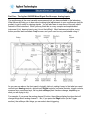
Part One – The Agilent 54622D Mixed-Signal Oscilloscope- Analog Inputs
The oscilloscope is the most versatile measurement tool you have available in the laboratory.
What follows will help you to learn about making initial adjustments to your oscilloscope (and its
probes), to get it ready for viewing signals. You will also learn to use some of the very useful
features of this instrument. While you may think this is a very complex and sophisticated
instrument (it is), learning how to use it is not that difficult. Most features are intuitive, every
button provides and immediate "help" screen, and you'll soon be very comfortable using it.
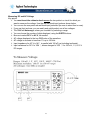
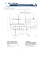
As you can see above, the front panel is logically laid out, making it easy to find what you need:
vertical input Analog controls, vertical input Digital controls, horizontal controls, trigger controls,
measure keys, waveform keys, file key and softkeys (their functions change, depending on
what you are trying to do).
For example, if you press the analog channel 1 button, the softkeys display functions that will
change things about analog channel 1. But, if you press the Edge button (in the Trigger
section), the softkeys offer things you can select about triggering.
3
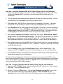
Basic Start-Up Procedure: (Refer to the picture of the oscilloscope front panel as you go
through this procedure).
1) Turn the oscilloscope ON by pressing the white button at the lower right corner of the CRT
screen (the graticule of the cathode-ray tube). You should see the “Startup Menu”, which
includes Softkeys (buttons directly under the CRT screen) labeled Getting Started, Using
Quick Help, About Oscilloscope, and Language. Try them all.
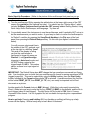
2) You probably weren’t the last person to use the oscilloscope, and it’s probably NOT set up to
do the measurements you want to make. A good way to start is to return the oscilloscope to
its “Default” condition by pressing the Save/Recall Hardkey in the File area of the front
panel, then pressing the Default Setup softkey. Do this now (see Agilent’s information
below).
You will now see a horizontal line in
the middle of the CRT graticule, and
at the top right is a blinking “Level”.
This area of the display is telling
you that the oscilloscope is
configured to trigger its sweep on
Channel 1, using positive edge
triggering in Auto Level mode, and
it’s NOT finding a signal at the
trigger Level of 0.00 V. This makes
sense, as there is no input signal at
this time.
IMPORTANT: The Default Setup does NOT change the how waveforms are saved to a floppy
disk. You should be sure to check that your oscilloscope file format for saving waveforms is TIF
(tagged image file). This can be selected by using the Utility hardkey, then the Print Confg
softkey followed by the Format softkey where TIF is selected. A saved waveform (the first one
will be called PRINT_00.TIF, then PRINT_01.TIF, etc.) can easily be imported into a Word
document as a picture.
Another graphic file Format choice is BMP (bitmap). While this is also easily imported into
Word, it takes twice as long to write the file (e.g. PRINT_01.BMP) to the diskette, and the file is
much bigger (about 6 times bigger!). The last choice for file format is CSV; this is CommaSeparated Value format. It is not a graphic file, but is suitable for importing into a spreadsheet
program.
How to get help: Pressing and holding ANY key (hardkey or softkey) will bring up a help
screen on the display. What a handy way to learn about its features!
4
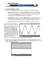
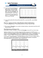
3) QUICK PERFORMANCE CHECK:
Connect a 10X attenuating probe to Channel 1. Change three (3) settings as follows:
a) Vertical Section: Channel 1, change Probe Factor (a softkey that says Probe) to
10:1. You can do this by pressing the oval button labeled “1”, and then turning the
control called the “Entry Knob”, located just to the right of the CRT, below the
horizontal section, with an illuminated curved arrow above it.
b) Vertical Section: Channel 1, change to 500 mV/div scale. You can do this by
pressing the oval button labeled “1”, and then turning the control right above the oval
button and observing the vertical scale (at the top left side of the CRT screen).
c) Horizontal Section: change time/division to 5 ms/div, using the larger control.
Now, touch the probe tip with your
finger. If you see a few cycles of a
sine wave with several cm of vertical
deflection (like the display to the
right), both your oscilloscope and
your probe are functioning. Note:
you may need to use 200 mV/div or
1V/div, depending on where you are.
It turns out the “signal” you are
observing is 60 Hz. power line noise,
and your finger (which is most likely
connected to your body, a crude
antenna) is providing a very
convenient “test” signal picked up from the power wiring in the building.
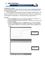
4) Connect the Channel 1probe tip to the Probe Comp output (near the right edge of the front
panel). The display should look like the display below: not very satisfactory, but you can see
there’s some kind of waveform.
5
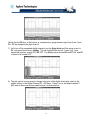
5) Three controls need to be adjusted to give a satisfactory display: the Vertical Section
volts/div and position, and the Horizontal Section time/div. These controls can be
adjusted two ways: by YOU, or by the oscilloscope.
For now, let’s have the oscilloscope do the adjustment. Press the Autoscale hardkey, a
white button just above the Vertical Section. You should see a display very similar to the
one below with about 2_ cycles of the squarewave (although the corners may not look quite
so square as they do below).
Note that a softkey called Undo Autoscale has appeared at the lower left of the display.
This can be a very valuable and time-saving button to use, under certain circumstances. Try
“undoing autoscale” by pressing this softkey button. Then, press the Autoscale hardkey
again, and you should see about 2_ cycles of the squarewave.
The next step (number 6, Probe Compensation) is so important it has an entire
page devoted to it.
6
6) PROBE COMPENSATION: This step is a “MUST DO” procedure, each and every time you
turn on an oscilloscope. In fact, you must do it if you move a probe from one channel to
another, and especially from one ‘scope to another ‘scope (for example, from the analog to
the digital ‘scope).
If you don’t make sure that each probe is compensated properly, you can wind up with
incorrect waveforms and major measurement errors. The error can be seen immediately
with pulse waveforms (like the squarewave shown below), but does NOT show up at all for
sinusoidal waveforms (AC signals). All measurements of AC signal amplitude and phase
can have big errors if compensation is not done!
In fact, performing probe compensation is so important that oscilloscope manufacturers put a
“Probe Adjust” or “Probe Comp(ensation)” output voltage on the front panel of most
oscilloscopes.
PROBE COMPENSATION PROCEDURE:
a. Turn on the oscilloscope.
b. Connect a 10X probe to the Vertical
Channel 1 BNC input connector, and
connect the probe tip to the Probe
Comp output on the lower right side
of the front panel.
c. Press the Save/Recall key, then
press the Default Setup softkey
under the display.
d. Press the Autoscale key on the front
panel. You should now see a square
wave, with 5 divisions peak-to-peak
vertically.
e. Check the waveform presentation for overshoot and rolloff (see Figure above). If necessary,
adjust the probe compensation screw on the probe assembly for flat tops on the
waveforms.
f. Disconnect the probe connected to Channel 1, and set it aside. Connect the other 10X
probe to the Vertical Channel 2 BNC input connector.
g. Press the Autoscale key on the front panel. You should now see a square wave, with 5
divisions peak-to-peak vertically.
h. Check the waveform presentation for overshoot and rolloff (see Figure above). If necessary,
adjust the probe compensation screw for flat tops on the waveforms.
Make sure that both probes, for Channel 1 and Channel 2, are properly compensated
before proceeding.
7
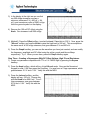
Features to Try - Vectors:
The 54622D oscilloscope is a digital instrument that makes a graph of voltage versus time by
putting individual dots on the screen. By contrast, an analog ‘scope creates a graph which is
continuous (no dots are used).
Each dot represents an (x,y) pair (time, voltage) in a Cartesian coordinate system. If the
dots are close together, your eyes are fooled and you see a continuous line; if the dots are too
far apart, you’ll see individual dots. To overcome the problem of seeing dots, a Vectors mode
can be used which “connects the dots”. This can be seen very clearly as follows.
YOU DO IT:
1) Press the Run/Stop button, so that it changes from green (Run) to red (stop). The
waveform displayed, and its dots, are now frozen in memory.
2) Change the Time/Div from 200 us/div to 20 ns/div. You should see the display below
(Vectors turned ON).
3) Now press the Display hardkey (in the Waveform section), and press the Vectors
softkey. Now the display (Vectors turned OFF) should appear. The individual dots
are very apparent, and this is not as “pleasing” a display. Normally, Vectors can be
left ON.
Vectors turned
ON
Vectors turned
OFF
8
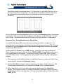
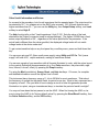
Features to Try - Averaging:
Our building, and most laboratories, are “dirty” in the electromagnetic sense. This is due to the
power line noise, computer systems, lighting, and RF (radio-frequency) signals that create
unwanted voltages on top of the voltages we do want to measure.
One way to minimize the problem (clean up the “dirt”) is to use the Averaging feature of
a digital ‘scope. Look closely at the waveform below, on the left. It is the Probe Comp
squarewave, and shows a “fat” line for the upper and lower parts of the square wave. This is
caused by the noise voltage superimposed on top of the signal voltage.
In the waveform below on the right, Averaging has been turned on, using 8 averages. Note
that the tops and bottoms of the square wave are much “thinner” (i.e. less noise is present),
because the noise has been averaged out of the display.
Probe Comp Signal, With Averaging
Probe Comp Signal, No Averaging
YOU DO IT: Now try it yourself, using the probe compensation signal on the front panel.
1) Get back to the basic factory default settings, use Autoscale and look at the Probe Comp
waveform. You should see the display shown above on the left (averaging is OFF now).
2) Press the Acquire hardkey in the Waveform section of the front panel, and turn on
averaging by pressing the Averaging softkey. You should now see the display shown above
on the right (averaging is ON).
Note that the number of averages (# of Avgs) can be changed, as needed, over a wide range of
values (the default number is 8). This feature may create problems. To see the effect of a
large number of averages, do the following:
3) Turn averaging OFF (by pressing the NORMAL softkey). Remove the probe tip from the
Probe Comp output, then reconnect it. Note the nearly instantaneous change in the display
(from squarewave to flat line).
4) Now turn averaging ON and set the # of Avgs to 8. Remove the probe tip from the Probe
Comp output, then reconnect it. Note that the change in the display (from squarewave to flat
line) is rapid, but gradual (i.e. it is not instantaneous). Leave the probe disconnected.
9
5) Leave averaging ON and set the # of Avgs to 4,096. Connect the probe tip to the Probe
Comp output. Note that the change in the display (from flat line to squarewave) is very slow
indeed. QUESTION TO PONDER: If time base is set to 200 µs/div, and there are 10
divisions on the graticule, how long does it take before 4,096 complete “sweeps” have
occurred? This is the time needed for the display, with squarewave removed, to become a
flat line, if one sweep begins right after the prior one ends. Turn averaging OFF (by
pressing the NORMAL softkey) when done with this step.
Features to Try - Using Cursors to Measure Time & Voltage:
In the “good old days”, the user of an analog ‘scope spent a lot of time measuring key
parameters of a waveform by counting divisions. The number of horizontal divisions gave
information about time (the period of a waveform, or pulse width, or time difference between two
waveforms). The number of vertical divisions told the user how big the voltage was (peakpeak, maximum, minimum, average value, etc.).
Let’s do some measurements by manually positioning the cursors on our Probe Comp
waveform.
1) Connect Channel 1 probe to the Probe Comp output terminal, and press the Autoscale
hardkey.
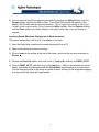
2) Press the Cursors hardkey, and you will see the waveform and softkey labels as shown
below in the left picture:
In this picture note that the (X Y) softkey
has X checked, and both the X1 and X2
cursors (dashed vertical lines) are at 0.000s
(this is the horizontal center of the display).
3) Press the X2 softkey, and turn the Entry Knob to move the X2 cursor to the rising edge
nearest the right side of the display.
Now the X1 cursor is at 0.000s, the X2
cursor is at 836.0us, and ∆X = 836 – 0.00 =
836 us. Frequency = 1/∆X = 1.1962 kHz.
10
4) Now press the (X Y) softkey, which will make the Y checked, and both the Y1 and Y2
cursors (dashed horizontal lines) are at 0.00V (this is the bottom of the waveform).
5) Press the Y2 softkey, and move the Y2
cursor line to the top of the waveform by
using the Entry Knob. Now Y2 is about
4.94 V, and the ∆Y = 4.94V. Your display
should look like the one on the right.
Features to Try - Using “Quick Meas” to Measure Time & Voltage:
As you just found, manually positioning the cursors on a waveform can give you important
information about a waveform. Since these kinds of measurements need to be done all the
time, your oscilloscope is designed to make many common measurements automatically.
These include:
Frequency, period and peak-peak voltage
Maximum, minimum, rise time, fall time and duty cycle
RMS (root-mean-square or effective value), +width, -width, average and amplitude
Top, base, overshoot, preshoot, and X at Max
Phase shift (Ch. 1 compared to Ch. 2), time delay (Ch. 1 compared to Ch. 2)
Let’s do some measurements now using the “Quick Meas” feature.
1) Connect Channel 1 probe to the Probe Comp output terminal, and press the Autoscale
hardkey.
2) Press the Press the Quick Meas hardkey. You will see the display below. The ‘scope has
determined that the frequency is 1.199 kHz, and the peak-peak amplitude is 5.19 Vpp.
11
What is wrong with the amplitude value of 5.19 Vpp is that it is a bit wrong (too big), due to
the noise on the Probe Comp signal. You can see that the dashed horizontal cursor lines
are positioned above and below where they should be (on the top and bottom of the
waveform).
Get rid of the noise by pressing Acquire hardkey, and then the Averaging softkey (and average
8 waveforms). We can see that with averaging on, the amplitude is now 4.979 Vpp, 4 % lower
than 5.19Vpp. The dashed cursor lines now lie right on the top and bottom of the waveform.
Features to Try – Saving Waveforms to a Floppy Disk:
The Default Setup does NOT change the how waveforms are saved to a floppy disk. You
should be sure to check that your oscilloscope file format for saving waveforms is TIF. This can
be selected by using the Utility hardkey, then the Print Confg softkey followed by the Format
softkey where TIF is selected.
Another graphic file Format choice is BMP (bitmap). While this is also easily imported into
Word, it takes twice as long to write the file (e.g. PRINT_01.BMP) to the diskette, and the file is
much bigger (about 6 times bigger!). The last choice for file format is CSV; this is CommaSeparated Value format. It is not a graphic file, but is suitable for importing into a spreadsheet
program.
1) Get a waveform on the display, perhaps by connecting Channel 1 probe to the Probe Comp
output terminal, and press the Autoscale hardkey.
2) Use the Quick Meas hardkey to measure frequency, peak-peak voltage, and period. The
first two happen automatically; you must press the Period softkey to measure period.
3) With a floppy disk in the 3.5-inch disk drive under the display, press the Quick Print
hardkey. The displayed waveform, including the frequency, peak-peak voltage, and period,
will be written to a file on the floppy disk. If it’s the first waveform saved, the file will be called
PRINT_00.TIF.
12
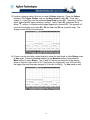
4) You can see that the file was saved successfully by pressing the Utility hardkey, then the
Floppy softkey, and then the File: softkey. A list of the file(s) saved will appear on the
display, with the date and time they were written. This is a good opportunity to see if your
‘scope’s clock is set correctly; if it isn’t, press the Utility hardkey, then the Options softkey
and the Clock softkey and make changes to the year, month, day, hour and minute as
needed.
Importing Saved Waveform Displays into a Word document:
This can be done either in lab (if a PC is available) or at home.
1) Insert the floppy disk containing the stored waveform(s) into a PC.
2) Open a Word document (new or existing).
3) Click on Insert in the toolbar at the top of the screen, and move the cursor arrow down to
Picture.
4) Choose the From File option, and Look In the 3_ Floppy (A:) directory for PRINT_00.TIF
5) Click on PRINT_00.TIF, and then click on the Insert icon. Within a few seconds the saved
display (waveform and data measured with Quick Meas) should appear in your document.
You can change the size of the image a number of ways: clicking on the image and dragging
a corner inward will make the image smaller.
13
HANDY HINTS:
Pressing and holding ANY key (hardkey or softkey) will bring up a help screen on the display.
This is a great way to learn about oscilloscope features.
Softkeys are at the bottom of the display. They will appear when a Hardkey is pressed.
DON’T use the oscilloscope to delete files on your floppy disk, except files that IT created.
Autoscale may not give a desirable result; use Undo Autoscale if this happens.
When you use Autoscale, the ‘scope looks for repetitive waveforms 10 mVpp or larger, a duty
cycle greater than 0.5%, at no less than 50 Hz, and will turn off any channel not meeting those
criteria. It will choose as its trigger source whichever of these has a valid signal on it, in the
order listed: External Trigger, Channel 2, then Channel 1.
If you have signals on channels 1 and 2, when you use Autoscale the ‘scope automatically
chooses channel 2 as the trigger source. You may need to manually change the trigger source
to channel 1.
Measurements made with Quick Meas may give incorrect results, particularly on noisy signals.
Look carefully at the cursor lines to see if you agree that the cursor lines are showing what you
want to measure. If your displayed signal is noisy for any reason, try using Averaging to clean
it up. If the noise is too big to eliminate with Averaging, using manual cursors to make your
measurements.
The Entry Knob (at the right side of the display) is used to change many settings, depending on
which Softkeys are showing.
Be sure the Probe value (attenuation factor) for both channels is set correctly for your probes.
Every time you return the oscilloscope to Default Setup, the probe attenuation factor is set to
1.0:1. You must change it back to 10:1 (assuming you are using 10X probes).
You can move the trigger point, which is the center of the graticule by default, using the
Main/Delayed hardkey and the Time Ref softkey.
The intensity of the grid on the graticule may be changed by pressing the Display hardkey and
using the Grid softkey.
You can save a “setup”, which stores the waveforms, cursors, math measurements, horizontal,
vertical and trigger settings to a floppy disk or to an internal oscilloscope memory. When you
recall that information, you can elect to restore the setup, or the waveform trace, or both.
14
Part Two – The Agilent 54622D Mixed-Signal Oscilloscope- Digital Inputs
Features to Try - Turning On the Digital Channels
1) OK, now that we are familiar with the mixed-signal oscilloscope using its analog inputs, now
let's get acquainted with the digital inputs and their controls.
2) First, return the oscilloscope to its “Default” condition by pressing the Save/Recall Hardkey
in the File area of the front panel, then pressing the Default Setup softkey.
3) Next, connect a (compensated) 10X analog probe from channel 1 input to the Probe
Compensator output (probe tip to "Probe Comp", probe ground the the ground connection
immediately above.
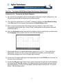
4) Press the Autoscale hardkey, and adjust the display so that it looks like the one below (note
that Averaging is being used to remove noise from the waveform):
What we see above is a unipolar squarewave, going from 0 V to 5 V. This sounds like a
digital signal, and we can use it to try out the digital input capability of the mixed-signal
oscilloscope (using just one of the 16 digital input channels).
5) Connect the 16-channel cable (part of the digital probe kit) to the D15-D0 input connector on
the front of the oscilloscope.
6) Connect the D0 lead to the "Probe Comp" output (where the 10X probe tip is still connected).
Now press the D7 Thru D0 hardkey in the digital section of the front panel, and you should
see analog channel 1 on the top of the display, and eight digital channels (D0 - D7) on the
bottom. See the display below:
15
Notice that the D0 line, at the bottom, is a squarewave, going between logic level 0 and 1,and
D1 - D7 are straight lines (logic level 0).
7) Let's turn off the unneeded digital channels: turn the Entry Knob until the arrow is next to
D1, and press the left-most softkey. This will toggle D1 on and off. Leave it off. Now,
repeat this process, turning OFF D2 - D7. The display below shows D0 and D7 ON, and D7
is about to be turned OFF.
8) The last control we may want to change is the size of the digital channel(s), which is the
middle softkey in the Digital Channel D7 - D0 Menu. Press it once, and digital channel 1
(D1) now is about one division peak-to-peak, as shown below.
16
Note that using the Digital Channel Position control (directly under the D7 Thru D0
hardkey) we can move the D0 display up and down on the screen, as needed. Also look at
the top of the graticule in the display above; the D7 _ _ _ _ _ _ _ ¤ D0 box shows that D7 D1 are turned OFF, and that D0 is going between logic 1 and 0.
9) If you have a 4-bit counter available (e.g. a TTl 7493 IC or CMOS CD40161 or CD4024use 4 of the 7 bits), connect the input to a suitable oscillator. Then, connect digital
channels D0 - D3 to the counter output, with D3 going to the MSB (most significant bit).
10) Press the AutoScale button, and you should see a display somewhat like the one below:
11) Triggering can be a bit tricky at first, and AutoScale doesn't always make a triggering
choice that will give a "good" display. For example, in the display above of D0 - D3, the
trigger source chosen is D2 (with positive edge triggering), and the D3 waveform is
jumping around.
12) Press the Edge hardkey in the Trigger section, and rotate the Entry Knob to select D3
as the trigger source (as shown below). Since D3, the MSB, is the lowest frequency of
the four digital channels, a stable display will result.
17
13) Another triggering method that can be used is Pattern triggering. Press the Pattern
hardkey in the Trigger Section, and use the Entry Knob to select D0. Press the L
softkey (L = logic Low), and the rotate the Entry Knob to select D1. Press the L softkey
again, and select D2; again press the L softkey. Lastly, Select D3, and press the up
arrow ( ↑ ) softkey, to choose positive-edge triggering on channel D3. This process will
now make the trigger occur when D2 - D0 are Low, and D3 has a positive edge. The
display should look like the one below.
14) Cursors can be used with a digital display to show the logic levels in either Binary mode
or Hex mode. Press the Cursors hardkey (in the Measure section), then press the
Mode softkey to select Binary. The X1 and X2 cursors are positioned in the display
below to show the logic values of 0111 just before the trigger point, and 1000 just after
the trigger (the time base was changed to 10 ms/div for clarity). Try Hex mode as well.
18
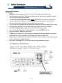
Part Three – The Agilent E3631A Power Supply
A power supply is used to provide DC voltage(s) needed by a circuit that doesn't supply its own
power. The Agilent E3631A is actually three power supplies:0 to 6 V, 0 to 25 V, and 0 to -25 V.
In this section you will see how to set the voltage of each supply and how to use "current
limiting" on each supply to protect your circuit.
19
Setting the voltage limit is quite simple to do, and to understand. Refer to the front panel picture
on the previous page, and the instructions below.
Setting the Output Voltage:
Let's say you have built a circuit that needs +5 V. So, you follow the process above to set the +6
V supply to +5.000 V. Do this now, and verify that the output voltage is 5.000 V.
Or, your circuit needs +/- 15 V, in which case you follow the process above to set the +25 V
supply to +15.00 V, and the -25 V supply to -15.00 V. Do this now, and verify that the voltages
are +15 V and -15 V (both measured with respect to the black COM terminal).
However, taking the time to also set the current limit can be a really smart precaution, in case a
wiring error, defective component, or accidental connection (e.g. bridging two pins on an IC)
during testing would cause excessive current to flow and damage your circuit. The +6 V supply
can source 5 amperes, and the +/- 25 V supplies can source 1 amp; this is a substantial amount
of current, and can create a lot of smoke and damage to components in your circuit.
20
Setting the Current Limit:
1) Let's assume you have set the +6 V supply to 5.000V, and the display indicates you have the
+6 V supply selected. To set the current limit, press the Display Limit button, then the
Voltage/Current button. Use the control knob and the "Resolution Selection Keys" (the <
and > keys underneath the control knob) to adjust the current limit to 0.020 A.
2) This setting of 0.020 A means that no matter what you do, the current from the +6 V supply
(which is now set to 5.000 V) will never exceed 20 mA. Let's verify that two ways: with a
short circuit, and with an LED.
3) First, note the voltage and current displays: the voltage is very close to 5.000 V, and the
current is 0.000A (since nothing is connected to the + and - terminals of the 6 V supply).
Also, at the right side of the display a "CV" is showing; this means the supply is in "Constant
Voltage" mode, and will maintain 5.000 V unless the current reaches 20 mA, in which case
the output voltage will drop to whatever value is needed to keep the current at 20 mA.
4) Connect a jumper wire (or alligator lead) between the + and - terminals of the 6 V supply.
Note the voltage is 0.000 V, the current is close to 20 mA, and the "CV" has been replaced
by "CC" ("Constant Current").
5) Now let's try this with an inexpensive LED. Connect an LED with the anode to the plus
terminal, and the cathode to the minus terminal, of the 6 V supply (which is set to 5.000 V).
Normally, without current limiting, an LED will be quickly destroyed by this procedure. What
happens to your LED?
What is the output voltage (it should be around 2.0 V, depending on the color of the LED)?
What is the current (it should be near 20 mA). Your LED is emitting light, and will live to see
another day, because the current limiting circuit protected it by lowering the voltage.
6) If you don't mind destroying an LED, you can see the effects of not using current limiting.
Turn the power supply off, then turn it on again. Set the +6 V supply to 5.000 V, and again
connect the LED to the + and - terminals. What happened? LEDs will either burn out, or will
get really hot (don't burn yourself on the leads of the LED).
This power supply has many useful features, including remote control and the ability to store
and recall three setups from nonvolatile memory. Look in the Agilent manual for this instrument
for complete information.
21
Part Four – The Agilent 34401A Digital Multimeter
The DMM (digital multimeter) is a very important laboratory instrument. This section will show
you how to make three of the basic measurements: voltage, resistance and current. The
34401A has many capabilities beyond measuring V, R and I; consult the Agilent User's Guide
for information on measuring frequency, period, continuity & diodes, and using the many
features and functions of this DMM.
When you turn the DMM on, it will be in the "Power-On and Reset State":
Function
= DC volts
Input resistance
= 10M Ω (may be changed to 10G Ω ! for 100 mV, 1 V, & 10 V DC ranges)
Range
= Autorange
Resolution
= 5_ digits
22
Measuring DC and AC Voltage
Key points:
You must insert the voltmeter leads across the two points in a circuit for which you
want to measure the voltage. Use the red and black input jacks as shown below.
You can use the rear panel red and black input jacks also (be sure to select front or rear).
If you use front and rear, you can easily and quickly select one of two voltages.
The DMM will Autorange, unless you override it by selecting a range.
You can choose the number of digits displayed, using the DIGITS buttons.
Be sure to select DC V or AC V, as needed.
AC voltage displayed is the true RMS value of the waveform.
AC voltage is accurate to less than 1% up to 100 kHz.
Input impedance for AC V is 1M Ω in parallel with 100 pF (not including test leads).
Input resistance for DC V is 10M Ω, unless changed to 10G Ω ! for 100 mV, 1 V, & 10 V
DC ranges
23
Measuring Resistance
Key points:
NEVER measure resistance in a "live" circuit. Turn off all power to the circuit.
If an ohmmeter is used in a "live" circuit, at best you will get incorrect readings; at worst
you can seriously damage the DMM.
You must insert the ohmmeter leads across the two points in a circuit for which you
want to measure the resistance. Use the red and black input jacks as shown below.
Use the red and black input jacks (on the right) as shown below.
You can use the rear panel red and black input jacks also (be sure to select front or rear).
If you use front and rear, you can easily and quickly select one of two voltages.
The DMM will Autorange, unless you override it by selecting a range.
You can choose the number of digits displayed, using the DIGITS buttons.
Be sure to select Ω 2W (ohms, two-wire).
Ω 4W (ohms, four-wire) is a more complex measurement that gives greater accuracy by
eliminating the contact resistance (of the leads to the device under test).
Make sure your hands don't contact both test leads; if they do, then you're measuring the
device under test in parallel with you.
See User's Guide page 216 for the test current for each resistance range.
Use these two red
and black terminals.
24
Measuring Current
Key points:
You must insert the ammeter leads in series to measure current in a circuit.
Use the red and black input jacks (on the right) as shown below.
You can use the rear panel red and black input jacks also (be sure to select front or rear).
If you use front and rear, you can easily and quickly select one of two currents.
The DMM will Autorange, unless you override it by selecting a range.
You can choose the number of digits displayed, using the DIGITS buttons.
Be sure to select DC I or AC I to measure DC and AC current.
See User's Guide page 216 for the "Burden Voltage" for each current range.
25
Part Five – The Agilent 33220A 20 MHz Function/Arbitrary Waveform Generator (AWG)
Introduction
The Function Generator is the instrument that creates input signals used to test circuits and
systems in the laboratory. This section will show you how to create some basic waveforms
commonly used in the lab: sine, square, triangle and pulse waveforms, including DC offset.
The 33220A has a large number of capabilities beyond measuring these basic waveforms;
consult the Agilent User's Guide for information on capturing and using "arbitrary" waveforms,
noise, signals with AM, FM and FSK modulation, sweeping signals over a range of frequencies.
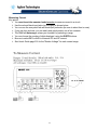
Operation of this "AWG" is easily learned, and fairly intuitive, as each front panel "hardkey" and
"softkey" (the buttons right under the display window in the picture below) when pressed for 2
seconds will provide context-senstive "help" on the display.
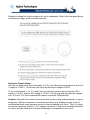
Output Voltage and the Load Resistance
Since this is a very important consideration, let's address it right now. Basic concepts:
You can easily set the amplitude and DC offset of the output waveform.
The output resistance of the AWG is always 50 Ω - this can't be changed.
If the AWG output connector is connected to a load (device under test) with a 50 Ω
resistance, then the amplitude and DC offset voltage values you set will be the values
across the load.
If the AWG output connector is connected to a load (device under test) with a high
resistance, then the amplitude and DC offset voltage values you set will NOT be the
values across the load. The output voltage will be twice what you set. This may
damage certain circuits (i.e. logic gate inputs).
You can tell the AWG that the load resistance is not 50 Ω. This will make the
displayed voltage (the one you set) and the open-circuit voltage the same.
We will practice using 50 Ω and "high Z" load resistances very soon.
26
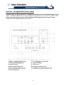
The Front Panel Controls
Refer to the diagram below as you perform the procedures that follow.
27
Step One - Creating a Sinewave With No DC Offset Voltage, High Z Load Resistance
1. A basic waveform you will now produce is a 1 kHz, 100 mVpp sine wave with no DC offset.
Connect the Output (a BNC connector on the front panel) to the vertical input of an
oscilloscope.
2. Turn the power on by pressing the white button at the lower left of the front panel. You are
reminded that you can get Help for any key by holding it down.
3. The display says 1.000,000,0 kHz, with a picture of a sinewave on the right. It also says
"Output Off", so the first thing we need to do is press the Output button. Press it now.
4. Press AutoScale on the mixed-signal oscilloscope (MSO) (or adjust its controls manually) to
display the sinewave. Press QuickMeas on the MSO to measure the frequency and peakto-peak voltage (should be very close to 1.000 kHz and 200 mVpp). You may want to turn
on Averaging on the MSO to minimize noise and get more accurate readings.
5. Now, press the Softkey labeled Ampl; it should say 100.0 mVpp. Wait a minute! What's
going on here - we just measured 200 mVpp? The reason for this discrepancy is that the
oscilloscope input resistance is 1M Ω (High Z), not the 50 Ω the AWG assumed was the
load resistance connected to the AWG output connector. How do we fix this discrepancy?
6. Since we are going to be using the MSO as our "Device Under Test" (i.e. the load connected
to the AWG), and the MSO resistance is 1M Ω, not the 50 Ω the MSO "expected", we will tell
the AWG what its load is.
7. Press the Utility hardkey, then the Output Setup softkey, and the Load softkey. This
changes the AWG to "High Z" mode, and it will now display the correct output amplitude.
8. Press the Sine hardkey; the amplitude now displayed is 200.0 mVpp, which agrees with the
amplitude as measured on the oscilloscope.
Be aware of the load resistance of the circuit or instrument you connect to the AWG. If you
were connecting the AWG output to a logic circuit (which could be damaged by an input voltage
that is too big) and did not change the AWG to "High Z" mode, the actual AWG output voltage
can be twice what the AWG display indicates.
Step Two - Creating a Sinewave With DC Offset Voltage, High Z Load Resistance
1) Leave the AWG in "High Z" mode. Now we will add some DC offset to our 1 kHz sinewave,
200 mVpp. This can be done two ways.
2) Method 1: Press the Offset softkey. Use the right "Navigation Arrow Key" to move the
cursor one place to the right on the amplitude display. Rotate the Knob one click
clockwise; this will add +100 mVDC to the 200 mVpp sinewave. See the display below.
28
3) In the display to the right we can see that
our 200 mVpp sinewave now has a
minimum value near 0 V (-400 uV = -0.4
mV), and a maximum value of 200.3 mVpp.
Note the ground symbol on the display.
4) Remove the 100 mV DC offset using the
Knob. Our sinewave is still 200 mVpp.
5) Method 2: Press the Offset softkey, to select LoLevel. Raise this to 0.00 V. Now, press the
"HiLevel" softkey, and use the Knob to raise the high level to 200 mV. This accomplishes
the same result: a 200 mVpp sinewave, that goes between 0 V and 200 mV.
6) Press the Graph hardkey; you can see the waveform you have just created, and can modify
the frequency, amplitude and DC offset using the yellow, purple and blue softkeys
respectively. Try it. When you are done, press the Graph hardkey again.
Step Three - Creating a Squarewave With DC Offset Voltage, High Z Load Resistance
1) Create a squarewave compatible with TTL or 5 V CMOS logic by pressing the Square
hardkey.
2) Press the Ampl softkey, which will turn it into HiLevel mode. Now use the Numerical
Keypad to enter: 5.00, then press the V softkey. You now have a 5 Vpp squarewave, which
goes between -2.5 V and + 2.5V. Verify this with the MSO.
3) Press the LoLevel softkey, and the
display will say -100 mV. Change this
with the Knob to be 000.0 mV. Your 5
Vpp squarewave, now goes between
0.0 V and + 5.0V. Verify this with the
MSO.
29
4) You can turn the squarewave into a
pulse train by pressing the Duty
Cycle softkey. Change the duty
cycle to 20% (the range is 20% to
80%), either using the Knob or the
Numerical Keypad. Your 5 Vpp, 1
kHz pulse train, goes between 0 V
and +5 V. Verify that yours looks
like the one to the right.
5) If you need a pulse with a duty cycle less than 20% or more than 80%, use the Pulse
hardkey
Step Four - Creating a Triangle or Ramp Waveform, High Z Load Resistance
1) Press the Ramp hardkey. The resulting waveform is a classic sawtooth shape.
2) By varying the Symmetry, you can make a triangle waveform, and sawtooth waveforms with
different shapes. Try it.
Other Waveforms and Features to Try
Noise (white, not pink) is available. Be sure that Averaging is turned off if you look at noise.
Arbitrary waveforms are non-standard voltages that either are stored in the AWG memory
("Built-In" waveforms) or that you capture and load into the AWG memory. Try pressing the Arb
hardkey, then the Select Wform softkey, then the Built-In softkey, and finally the Cardiac
softkey. To make it realistic, a human cardiac waveform should vary between approximately
0.33 Hz and 1 Hz (corresponding to 180 and 60 beats per minute). For now, to make it easy to
observe on your MSO, set the frequency to 20 Hz (representing, perhaps, a tachycardic
hummingbird after a double espresso); see the display below.
30
Other Useful Information and Review
As covered in the procedure, but of such importance that its repeated again: The output must be
terminated by 50 Ω for voltages set on the AWG to be accurate. OR, for loads that are much
higher resistance than 50 Ω, you can use the Utility key, then Output Setup softkey, and Load
softkey to select High Z.
The Help function tells us that "Load Impedance / High Z / 50Ω Sets the value of the load
attached to the [Output] connector (used for voltage settings). The Agilent 33220A has a fixed
series output impedance of 50Ω, regardless of the value specified for the parameter. If the
actual load is different than the value specified, the displayed voltage levels will not match
voltage levels at the device under test."
To get context-sensitive help on any front panel key or softkey menu, press and hold down that
key.
You can even get pure DC (like a small power supply) using Utility and DC On. This "power
supply" will have a 50Ω output resistance, making its usefulness limited.
You can see a graph of your waveform with all its parts illustrated, in color, with the colors keyed
to the controls that adjust those parameters (e.g. for a Pulse waveform, the pulse width, edge
time, HiLevel, LoLevel, offset), by pressing the Graph hardkey.
Try using the Mod (modulation), Sweep, Burst, and Help hardkeys. Of course, for complete
and detailed information consult the Agilent User's Guide.
This instrument has a frequency range of 1 µHz to 20 MHz for most waveforms. Think about
the frequency of sunlight on the planet Earth: its period is one day. What is that, expressed as a
frequency in hertz? Can you think of how to design a circuit to have this generator provide
illumination to a plant, using an incandescent lamp, to simulate the period of earth's sunlight?
You may not have been the last person to use the AWG. When first turning the AWG on, be
sure to return the AWG to its "factory default values" by pressing the Store/Recall hardkey, then
the Set to Defaults softkey, and the YES softkey.
31