Download Meade Image Processing Specifications

AutoStar
CCD Photometry
A Step-By-Step Guide
by
Jeffrey L. Hopkins
Hopkins Phoenix Observatory
Phoenix, Arizona
and
Gene A. Lucas
NiteOwl Astrophysical Observatory
Fountain Hills, Arizona
Modified DSI™ Pro CCD Camera with BVRI Photometric filters
On Meade 12-inch LX200 GPS Telescope
Copyright © 2007 Jeffrey L. Hopkins and Gene A. Lucas
All Rights Reserved
Reproduction or translation of any part of this work [except where
specifically noted] beyond that permitted by sections 107 or 108 of
the 1976 United States Copyright Act, without permission of the
Copyright Owner, is unlawful. Requests for permission or further
information should be addressed to: HOPKINS PHOENIX
OBSERVATORY, 7812 West Clayton Drive, Phoenix, Arizona
85033-2439 U.S.A.
First Edition – First Printing May 2007
Published in the United States of America
by Hopkins Phoenix Observatory
7812 West Clayton Drive
Phoenix, Arizona 85033-2439 U.S.A.
http://www.hposoft.com
__________
Adirondack Astro Video, All Electronics, and Scope Stuff are copyrighted©
trademarks® of their respective businesses. Astrodon and Schuler Photometric Filters are
copyrighted© trademarks® of Astrodon, Inc. ATIK is a copyrighted© trademark® of
ATIK, Inc. FileMaker Pro and FileMaker Developer are copyrighted© trademarks® of
FileMaker, Inc. Autostar Suite, Deep Sky Imager, DSI, DSI Pro, Envisage, LX200 GPS,
and the Meade logo are copyrighted© trademarks® of Meade Instruments Corporation.
Microsoft Office, Word, Excel, PowerPoint, and NotePad are copyrighted© trademarks®
of Microsoft Corporation. Sony HAD Ex-View is a copyrighted trademark of Sony
Corporation.
AUTOSTAR CCD PHOTOMETRY
i
Preface
There are at least two avenues to CCD photometry. First is for
someone who knows precisely what they want and digs into
learning how to achieve their goal. If they have previous
experience with single-channel photometry, the learning curve is
much easier. Another avenue to CCD photometry is for the
astronomer who starts with visual observing, moves to
astrophotography and then to CCD imaging. After taking many
“pretty pictures” this person decides there must be something more
that can be done with the equipment. Since the basis of CCD
photometry requires images being taken, this person has a “jumpstart” on learning CCD photometry. There is still a great deal to
learn in order to produce usable photometric data from the images,
however.
Many people are under the impression that a very expensive CCD
camera is needed. Certainly some of the upper-end CCD cameras
designed specifically for CCD photometry are excellent for the
purpose; however, the cost can be well out of sight for most
astronomers. Many people think you need a high-altitude, dark-sky
location to do useful photometry. This is not true. Unlike imaging
of faint deep-sky objects, most CCD photometry can be done
within an urban, light-polluted area. While it is true the darker the
location the fainter the stars you will be able to image, there are
many lifetimes’ worth of brighter objects just begging to be
observed.
Having worked with single-channel photometry for many years,
we decided to try CCD photometry, but without having to
mortgage our houses in order to buy high-end equipment. When
Meade Instruments came out with the monochrome Deep Sky
Imager DSI™ Pro for under $400, we decided that would be an
ideal CCD camera to work with. The price is well within the
budget of most astronomers, and the specifications for the camera
looked more than sufficient to experiment with CCD photometry.
In order to do filter photometry, we added a filter wheel and
standard BVRI photometric filters.
ii
AUTOSTAR CCD PHOTOMETRY
When purchasing a DSI Pro camera, the AutoStar Suite™
telescope control and imaging software is included at no additional
cost. While there are other CCD software packages on the market,
we decided to see just how useful the AutoStar software would be.
Although the Autostar documentation serves to get started in astro
imaging, it lacks detail in explaining what is needed to perform
photometry; and our first impressions were that we should
probably look to other programs. But since the AutoStar Suite
required no further investment, we decided to go ahead and
experiment with the included software. It turns out that the
AutoStar Suite is excellent and will do most everything required,
and has many additional features over some other CCD software.
Because the Phoenix, Arizona area tends to be very warm to
extremely hot (even at midnight) during the warmer months, the
ambient air-cooled DSI Pro camera produced higher dark counts
than desired. A simple and inexpensive modification to add a
thermoelectric cooler was developed, that has proved excellent in
not only reducing the dark noise, but also increased the camera
sensitivity.
After mentioning our success with the camera modifications and
AutoStar software to other astronomers, we received many
requests for more information. A web site was created with some
of the basics of what we had learned. This included step-by-step
Autostar procedures for performing astronomical photometry.
Then we decided to combine our skills and expand and share the
information – this book is the first result.
We hope this book will help to inspire others to try CCD
photometry. While the primary focus is on the Meade DSI Pro
cameras and AutoStar software, much of the information applies to
any CCD camera and associated computer programs. Once you
have set up your equipment and gained some experience, the
observations can be very rewarding. Indeed, you may even see
your name and data published in professional journals.
JLH and GAL, Phoenix, Arizona April 2007.
AUTOSTAR CCD PHOTOMETRY
iii
TABLE OF CONTENTS
Page
PREFACE
1. Introduction
1.1 Learning Stages
2. Data Acquisition
2.1 Telescope and Camera Setup
2.2 Software Setup
2.3 Setting Directories
2.4 Taking Dark Frames
2.5 Taking Stellar Images
2.5.1 Imaging Procedure
2.5.2 Flat Fields
3. Raw Data Reduction
3.1 Arranging the Files
3.2 Calibrating the Images
3.3 Differential Magnitude
3.3.1 Setting the Reference Magnitude
3.3.2 Aperture Diameter, Annulus, and Centering
Box Size Settings
3.3.3 Magnitude Determination
3.4 ImageInfo File
4. Additional Data Reduction
4.1 Database Program
4.2 Data List
5. Advanced Data Reduction
5.1 Reducing the Magnitudes to Standard Magnitudes
5.2 Transformation Coefficient Equations
APPENDIXES
REFERENCES
INDEX
i
1
1
3
3
3
5
6
8
8
15
17
17
18
21
21
24
24
26
27
27
28
29
29
29
31
103
107
iv
AUTOSTAR CCD PHOTOMETRY
TABLE OF CONTENTS – APPENDIXES
Page
A. Modifying a DSI Pro Camera
Introduction
The Affordable Meade Deep Sky Imager (DSI)
Monochrorme Deep Sky Imager Pro (DSI Pro)
Adding a Filter Wheel – Installing The Nose Piece Adapter
Filter Wheel
CCD Photometric Filters
Cooling the DSI Pro
TEC Cooler Mods
Parts List
DSI Pro TEC Cooler Modifications
Wiring and Schematics
Conclusion
List of Suppliers for Filters and Cooler Mods
B. Calculating the Air Mass
Introduction
Getting Started
Star's Declination (δ)
Determining a Star's Hour Angle (HA)
Determining Local Sidereal Time (LST)
Creating an LST Table Using MICA Software
LST Example
Determining the Hour Angle (HA)
Determining the Air Mass
C. Determining Standard Star Data
Observing Standard Stars in M67 (NGC 2682)
BVRI Standard Magnitudes in M67
D. Determining BVRI Extinction Coefficients
Introduction
Air Mass
Terms and Definitions
Equations
Instrumental Magnitude Calculations
Determining the Extinction Coefficients
Determination of Instrumental Magnitudes
33
33
34
34
35
36
37
39
40
41
41
43
44
44
45
45
46
47
48
49
50
52
52
53
55
55
58
59
59
59
60
60
60
61
62
AUTOSTAR CCD PHOTOMETRY
v
TABLE OF CONTENTS – APPENDIXES (Contd.)
Page
E. Determining BVRI Color Coefficients
Introduction
Air Mass
Terms and Definitions
Observational Data
Instrumental Magnitude Calculation
Extra-Atmospheric Calculations
Standard Star Magnitudes
Color Transformation And Zero Point Calculations
Coefficient Determination
Summary
F. Least Squares Method
Introduction
Equations
Plotting a Graph and Drawing the Straight Line
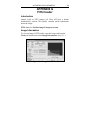
G. FITS Header
Image Information
Header Details
H. Light Box Design and Construction
Flat Fields
Light Box Construction Notes
Plans and Further Details
HPO Light Box
I. Suggested Projects
Introduction
Lunar Photometry
Solar Photometry
Planetary Photometry
Planetary Satellite Photometry
Comet Photometry
Stellar Photometry
Intrinsic Variables
Eruptive Variables
Extrinsic Variables
Nova and Supernova Photometry
Asteroid Photometry
J. References
INDEX
67
67
67
68
68
71
71
72
72
75
84
85
85
85
87
89
89
90
91
91
92
95
95
99
99
99
100
100
100
101
101
101
102
102
102
102
103
109
vi
AUTOSTAR CCD PHOTOMETRY
LIST OF FIGURES
Page
2-1. Meade AutoStar Suite Planetarium Screen -- Selecting
DSI Imaging.
2-2. AutoStar Envisage Screen -- Selecting Settings.
(Camera Not Connected or Inoperative).
2-3. Settings Window.
2-4. Selecting "Take Darks".
2-5. Take Darks Window.
2-6. Dark Frames Complete Window.
2-7. Envisage Screen With CCD Camera Operating.
2-8. Exposure Setting Window.
2-9. Deep Sky Image Process Window.
2-10. Save Process Window.
2-11. Quality and Evaluation Count Window.
2-12. Save Procedure Window.
2-13. DSI1 Folder Tab.
2-14. Tracking Star Selection Box.
2-15. Stats Area – (May Be Ignored for Photometry).
2-16. Long Exp and Live Selections. (Note Dark Sub is
Checked.)
2-17. Start Button
2-18. Sample I Filter Sky Flat.
3-1. Selecting a New Group of Images.
3-2. Selecting Filter Files to Calibrate with Flat Field.
3-3. Calibrate Selection.
3-4. Calibrate Window.
3-5. New Calibrated Image Files.
3-6. Photometry Cursor.
3-7. Select Set Reference Magnitude.
3-8. Set Reference Magnitude Window.
3-9 . Select Determine Magnitude.
3-10. Magnitude Determination Window.
4-1. FileMaker Pro Data Summation Program.
4-2. Database List of Data Records.
A-1. Modified DSI Pro CCD Camera and Filter Turret on
Meade 12 inch (30.5 cm) LX200 GPS Telescope at HPO.
A-2. DSI Pro Camera with Filter Slide (left) and Low-Profile
and Original Nosepiece Adapters (Right).
A-3. Disassembled ATIK Filter Wheel.
A-4. Filter Wheel Disk with BVRI Photometric Filters.
3
4
5
6
7
7
9
10
10
11
12
12
12
12
13
13
14
16
18
19
19
20
21
22
23
23
24
25
27
28
33
36
37
38
AUTOSTAR CCD PHOTOMETRY
vii
LIST OF FIGURES (Contd.)
Page
A-5. Standard UBVRI Johnson-Cousins Photometry Filter
Passbands.
39
A-6. Views Inside the DSI Pro with Cold Finger (White
Square) and Nylon Mounting Screws Shown.
41
A-7. Modified DSI Pro with Focal Reducer, Filter Wheel,
TEC/HeatSink/Fan Assembly and Foam Insulation.
42
A-8. Mechanical Modification Drawing and Electrical Schematic.43
B-1. Illustration of a Star's Air Mass (Accounting for Curvature
of the Earth’s Atmosphere).
46
B-2. Illustration of a Star's Declination.
48
B-3. Illustration of Star's Hour Angle for Northern Hemisphere
Observers Facing The Southern Horizon.
49
B-4. HPO FileMaker Pro Program for Calculating Air Mass.
54
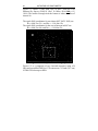
C-1. M67 Open Cluster Photograph.
56
C-2. M67 CCD Image Taken at HPO.
57
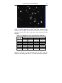
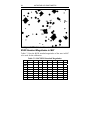
C-3. M67 Finder Chart for Star Identifications.
58
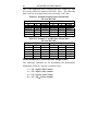
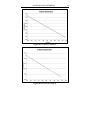
D-1. Plot of i versus X.
64
D-2. Plot of r versus X.
64
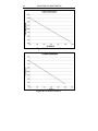
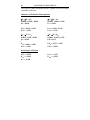
D-3. Plot of v versus X.
65
D-4. Plot of b versus X.
65
E-1 Example FileMaker Pro Observational Data Calculations. 69
E-2. Example FileMaker Pro Transformation Coefficient
Calculation.
70
E-3. ((V – I) – (v – i)o) versus (V– I) Plot.
76
E-4. ((V – R) – (v – r)o) versus (V – R) Plot.
78
E-5. ((R – I) – (r – i)o) versus (R–I) Plot.
78
E-6. (V – vo) versus ε * (B – V) Plot.
81
E-7. ((B – V) – (b – v)o) versus (B – V) Plot.
83
F-1. Manual Data Plot.
87
G-1. Image Information.
89
G-2. FITS Header.
90
H-1. Interior Construction of HPO Light Box.
95
H-2. Outside of Plywood Bulkhead with Aperture.
96
H-3. Inside of Plywood Bulkhead.
97
H-4. Typical Light Box Flat Field (V Filter).
98
H-5. Typical Twilight Sky Flat.
98
viii
AUTOSTAR CCD PHOTOMETRY
LIST OF TABLES
Page
3-1. ImageInfo Log Text File Example.
B-1. Part of a MICA Table Created for LST at HPO (Phoenix,
Arizona) for the Month of October 2005.
C-1. Sample Raw ADU Total Flux Data from M67.
C-2. M67 BVRI Standard Magnitudes.
D-1. Example I and R Observational Data for Star M67-081.
D-2. Example V and B Observational Data for Star M67-081.
D-3. Calculated Instrumental Magnitudes.
E-1. Observational Star Counts.
E-2. Instrumental Magnitude Calculations Summary.
E-3. Extra-Atmospheric Calculations (X=1.0809).
E-4. Equations and Extinction Values.
E-5. Standard Star Magnitude Data.
E-6(a). R-I Color Transformation Plot Calculations.
E-6(b). V-I and V-R Color Transformation Plot Calculations.
E-6(c). B-V Color Transformation Plot Calculations.
E-7. ((V – I) – (v– i)o) versus (V – I) Data.
E-8. ((V – R) – (v – r)o) versus (V – R) Data.
E-9. ((R - I) - (r - i)o) versus (R - I) Data.
E-10. (V – vo) versus ε * (B – V) Data.
E-11. ((B – V) – (b – v)o) versus (B – V) Data.
E-12. BVRI Color Transformation Coefficients.
E-13. BVRI Zero Points.
F-1. Sample Data.
26
51
57
58
62
62
63
68
70
71
72
72
73
73
73
75
77
79
80
82
84
84
86
AUTOSTAR CCD PHOTOMETRY
1
1. Introduction
Astronomical photometry performed with Charge Coupled Devices
(CCDs) has the big advantage of being able to acquire
simultaneous data on multiple stars. The sensitivity of the CCD
allows short exposures on the brighter stars, and also the ability to
work with very faint stars. One disadvantage is the low dynamic
range of the CCD camera, compared to single-channel photometry
such as using photon counting methods. For accurate CCD
photometry, the comparison and program stars must be within one
or two magnitudes of each other. Photometric imaging is very
similar to regular astro imaging, except the images are taken
through special photometric filters.
1.1 Learning Stages
1. Learning the equipment – telescope, mount, camera, and
software. While most any telescope can be used, reflectors are
favored. For the telescope mounting, a fork mount will be superior
to a German Equatorial Mount (GEM). This is because the best
photometry is performed near the meridian (straight overhead) and
that is where the GEMs are weakest, as they must do a “meridian
flip” to continue tracking past the meridian. A fork mount has no
such problem. A polar/equatorial mounted telescope is preferred to
an altitude/azimuth (Alt/Az) mount, although it is certainly
possible to do photometry with an Alt/Az mounted telescope. A
permanent setup is preferred. If the telescope and camera/filter
equipment is removed each night, setting up and aligning can take
a fair amount of time. Some protection against wind and stray light
is useful. But horizon-to-horizon visibility is not needed. At the
most, plus and minus 60 degrees (a cone of 120 degrees with the
telescope at the vertex) from the zenith would be fine. In fact, plus
and minus 30 degrees will work well most of the time, as that is
the best region for photometry.
2. Learning to take good images of star fields involves taking
Dark and Flat Fields and using them to calibrate the images.
2
AUTOSTAR CCD PHOTOMETRY
3. Practicing Photometry – Once you have mastered the imaging
steps, you are ready to practice photometry. Pick some stars that
are high in the sky when they cross the meridian. The closer to the
zenith, the better. The further from the meridian the poorer quality
the images will be and thus poorer photometry. Try to plan your
observing so that the star is to the East of the meridian and will
cross during the observing session.
4. Take multiple sets of images of a star field with a Program
and a Comparison star. Be sure to save the images as FITS. If you
save the images as a JPG or GIF or other than a FITS format, you
cannot do photometry on the image.
5. Practice getting data from a single image until you get
consistent magnitude values. The values should repeat exactly for
the same image. This may require investigation into the profile of
the star image and adjusting the Aperture and Annulus settings.
(These settings are discussed in later sections.)
6. Practice getting data from several images of the same star
field taken near the same time and with the same filter. The
magnitude data on the individual stars should be the same between
images. Most likely, the data will not be the same at first. Work to
find out why and how to minimize the differences.
7. Once you have repeatable data and are confident in knowing
what you are doing, start some serious photometry.
The following chapters describe suggested procedures for using a
Meade® Deep Sky Imager (DSI)™ Pro or DSI Pro-II monochrome
CCD camera with the AutoStar Suite™ and Envisage software.
Note: Aside from the specific steps involved in taking images with
the DSI camera, once images have been acquired with most any
CCD camera and stored as standard FITS files, the AutoStar Suite
Image Processing software can be used, and the rest of the
instructions for photometry also apply.
AUTOSTAR CCD PHOTOMETRY
3
2. Data Acquisition
Before any photometry can be done on the star, you must first take
suitable images. The following steps describe the procedures
developed at Hopkins Phoenix Observatory (HPO) using the
Meade® AutoStar Suite™ software and a DSI™ Pro or DSI Pro-II
monochrome CCD cameras to acquire photometric images.
2.1 Telescope and Camera Setup
Set up the telescope and DSI camera, and connect the cables to
your PC. Power up the telescope and align it for tracking. Be sure
to uncover the optics. Turn on the PC. (The following instructions
assume the Meade Autostar Suite Software has been installed.)
2.2 Software Setup
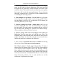
Click on the Autostar shortcut icon and Open the Meade AutoStar
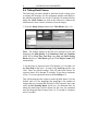
Suite software. The first window shown (Figure 2-1) is the
Planetarium (star map display) program. From the Image pulldown menu tab, select DSI Imaging.
Figure 2-1. Meade AutoStar Suite Planetarium Screen
– Selecting DSI Imaging.
4
AUTOSTAR CCD PHOTOMETRY
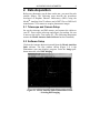
The AutoStar Envisage window will then open (Fig. 2-2). After a
few moments, if there are problems and the camera image doesn't
show up, check the USB connection to the DSI camera. You
should use a powered USB 2.0 interface, even though the DSI
camera will work marginally with USB 1.0. If problems persist, try
another USB cable. Note: A maximum length of 12 to 16 feet (3.5
to 5 meters) is recommended for the USB 2.0 cable connection to
the DSI camera.
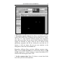
Figure 2-2. AutoStar Envisage Screen -- Selecting Settings.
(Camera Not Connected or Inoperative).
Figure 2-2 shows the AutoStar Envisage default window, the one
that displays when the camera is not recognized (not connected or
has a problem). This is easily identified by the "Add" and
"Remove" buttons at the upper left. When the camera is connected
and all is working, those are replaced by the "Gain" and "Offset"
sliders. (Also note that the window showing the camera image is
blank.) It may be necessary to re-connect the USB cable and
camera to a specific USB port, in order for the device to be
recognized.
AUTOSTAR CCD PHOTOMETRY
5
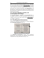
2.3 Setting Directories
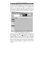
Before going further, you may wish to set the Settings for the
image acquisition program (Envisage) for your setup. Select the
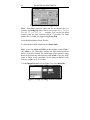
Settings pull-down menu (Figure 2-3).
Figure 2-3. Settings Window.
For the Image Directory and Dark Frames Directory, use the
default settings or create new ones. (To avoid confusion until you
have gained experience, it is suggested to use the default
directories.) Note: The Temperature boxes are merely a
Fahrenheit-to-Celsius conversion and do not do anything else.
Click OK when done.
Open the observatory, and set up the telescope and tracking. Turn
on the camera and start cool-down/stabilization. Allow 15 minutes
or more before proceeding.
6
AUTOSTAR CCD PHOTOMETRY
2.4 Taking Dark Frames
The following procedure should be performed each evening, prior
to starting the imaging. Let the equipment stabilize and adjust to
the ambient temperature for at least 15 (ideally 30) minutes before
doing this. Dark Frames are used in the software to subtract the
inherent noise in the camera electronics from the images.
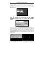
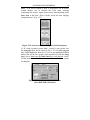
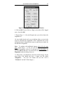
1. From the Image Process menu select Take Darks. (Fig. 2-4.)
Figure 2-4. Selecting "Take Darks".
Note: The default display in the blue area changes for the one
displaying the Min Quality %, Evaluation Count and Combine
check box to First Exp, Last Exp, Avg Exp and Del Existing
Darks check box. Take Darks gets put in the Object Name field
automatically.
2. Set the range of exposure times. The shortest is 1.0 seconds. Set
the First Exp (in this case 1.0), and set the Last Exp (in this case
30.0). These are default settings. This will take Dark Frames for
exposure times of1.0 through 30 seconds. If you plan a maximum
of say, 15-second exposures, then set the Last Exp to 15.
This will shorten the time it takes to make the dark frames. Use the
default value of 5 for Avg Exp (the Avg Exp is the number of
images that are averaged and stacked for each exposure time) and
select the Del Existing Darks check box. An estimated time for
taking the dark frames will be shown (for this case, the estimated
time for taking the Dark Frames from 1 to 30 seconds is 8 minutes
and 32 seconds).
AUTOSTAR CCD PHOTOMETRY
7
Note: There will be one Master Dark Frame for each exposure 1.0
second or greater (for the times used). You cannot take Dark
Frames for exposure times less than 1.0 second; and indeed they
normally are not needed for such short exposures. Filters do not
enter in for Dark Frames. Since Bias data is part of the Dark
Frame, there is no need to take separate Bias Frames. The filter
selected does not matter. There may be some light leakage through
the filter wheel (or slider), so it is best to do this after it is
completely dark. (If necessary, say if the Moon is very bright,
cover the filters with a dark cloth.)
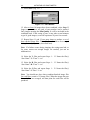
3. Click the Start button. A Take Darks window will pop up,
telling you to cover the telescope objective. (Fig. 2-5.)
Figure 2-5. Take Darks Window.
4. Cover the front of the telescope and click the OK button.
5. The computer will take the Dark Frames automatically. When
completed, a Dark Frames Complete window will pop up,
reminding you to uncover the telescope. (Fig. 2-6.)
Figure 2-6. Dark Frames Complete Window.
6. Uncover the telescope and click the OK button.
8
AUTOSTAR CCD PHOTOMETRY
You now have a set of Master Dark Frames for the desired
exposure times. These are stored in a folder called Darks located
in the Meade Images folder (unless you designated a different
folder).
2.5 Taking Star Images
When taking stellar images for photometry, one of the great
features of CCD imaging with the Autostar Suite software is the
ability to automatically take multiple short exposure images and
stack them. The images can also be automatically aligned with the
software. While a single, long-exposure (say, 60 seconds) might be
considered to be better than 10 each 6-second exposures, the
shorter exposures have advantages. One big advantage of stacking
multiple images is that the signal-to-noise (S/N) ratio is improved,
while also minimizing any tracking errors.
2.5.1 Imaging Procedure
1. Find the star field to be imaged and center the telescope on the
first star. Position the B filter in the optical path. If you are using
an SCT telescope equipped with a mirror lock and an external
electric focuser, set the fine electric focus so that the range of
movement is about midway between the extremes. Now do a
(normal) coarse focus with the telescope manual focuser (the knob
that moves the primary mirror). Turn (or drive) the knob CCW
past the focus and then CW back to the focus. (Always finish by
moving the focus in the same direction.)
Now Lock the mirror (if the telescope has a Mirror Lock). Final
focus using the fine motion electric focuser for the sharpest images
with the CCD camera.
Figure 2-7 shows a screen shot with the DSI Pro CCD camera
connected and working. Check the focus in each of the filters. At
HPO, we have found that imaging with the I filter seems to be the
most critical. If that is focused well, the other filters are usually
acceptable also.
AUTOSTAR CCD PHOTOMETRY
9
Figure 2-7. Envisage Screen With CCD Camera Operating.
2. Determine exposure time(s) that allows reasonable maximum
count values for the stars of interest, but less than 65,535 counts.
(See Fig. 2-7.) This includes both the program and comparison
stars, and in each filter. Do not worry if some of the other field star
images are saturated. As long as they are not of interest (in the
photometry program) and do not overlap the stars that are of
interest, it will not matter. Do not pay any attention to the
histogram or other items in the Stats area.
Remember, different filters can have different exposure times.
Make sure the Gain and Offset are at the default settings of 100
and 50, respectively. At these settings, a count of less than 65,535
will be in the linear region of the CCD.
3. Set the exposure time. Figure 2-8 shows a screen shot of the
area where you can set the exposures.
10
AUTOSTAR CCD PHOTOMETRY
Figure 2-8. Exposure Setting Window.
Note: Live Exp exposure times can be set shorter than 1.0
seconds; and Long Exp times can be set to steps of 1.0, 1.4, 2.0,
2,8, 4.0, 5.7, 8.1, 11.3, 15, .... seconds. You can use the Live
exposure time for short exposures (up to 15 seconds). For times
greater than 1 second, we suggest using Long Exp.
Leave the Live button clicked for now.
4. Check the dark field subtraction box (Dark Sub).
Note: Leave the Gain and Offset at their default values (Gain =
100, Offset = 50). With these settings, the DSI camera produces
about 1.43 ADUs/electron. The linear range of the camera is up to
about 45,000 electrons; which means with a Gain of 100, the ADU
count is linear to the maximum 16-bit analog-to-digital (A-D)
converter output, or 65,535 counts.
5. In the Image Process box (see Figure 2-9) select Deep Sky.
Figure 2-9. Deep Sky Image Process Window.
AUTOSTAR CCD PHOTOMETRY
11
6. File Naming -- Note: CCD photometry imaging creates an
enormous amount of data very quickly. Each image will be over
1.2 MB. It is very important to develop a systematic approach to
handling the data and naming of the files. The following
procedures is what is used at HPO and is just a suggestion. You
can develop your own technique as long as it works for you.
In the Object Name field (Fig. 2-7), change the name from “Deep
Sky” to the name of the image file for the exposure, e.g., “Star
Name”-I-“exposure time”-“Set No.”-, e.g., “TO-I-4-3-”.
Note: The software will automatically add a sequential number to
the end of the file name (e.g., TO-I-4-1-1, TO-I-4-1-2, TO-I-4-1-3,
etc. The next set would be TO-I-4-2-1, ...). You cannot use a
period in the file name. So for exposure times with a decimal
value, just specify the exposure time without the period; i.e., 28
stands for 2.8, 40 for 4.0, 57 for 5.7, or just use 4 for 4 seconds
etc., dropping the zero where appropriate.
7. Click the Save Proc... button. The Save Process window will be
shown as seen in Figure 2-10. Make sure for File Type that "Fits"
is selected. For Save Options make sure "Normal Operation" is
selected. Leave the Single Shot and Web Mode buttons
unchecked. Click OK.
Figure 2-10. Save Process Window.
12
AUTOSTAR CCD PHOTOMETRY
8. Unless the sky is exceptionally steady, leave the image quality
(Min Quality %) at 30 and evaluation frames (Evaluation Count)
at 5. These default values seem to work well. Check the Combine
box. (Fig. 2-11.)
Figure 2-11. Quality and Evaluation Count Window.
Make sure the images are saved as FITS files and Normal
Operation is selected (see Fig. 2-12). Click the Save Procedure
button.
Figure 2-12. Save Procedure Window.
9. Now we will set up a Tracking Reference Star that will be
used to align the images in the stack of images that are combined.
While viewing the real-time image (with the DSI1 folder tab
selected and Live box checked; see Figure 2-13), draw a small box
around an isolated star to be used as a Reference Guide Star (see
Figure 2-14).
Figure 2-13.
DSI1 Folder Tab.
Figure 2-14.
Tracking Star Selection Box.
AUTOSTAR CCD PHOTOMETRY
13
Note: If an Alt/Az mount is used, a second box can be drawn
around another star to derotate the field when stacking
(combining) the images. Again, do not worry about anything in the
Stats Area at this time. That is mostly useful for astro imaging
(not photometry). (Fig. 2-15.)
Figure 2-15. Stats Area – (May Be Ignored for Photometry).
10. If a long exposure (greater than 1 second) is used, make sure
the Long exp check box is selected. (Fig. 2-16.) Set the Long exp
time, and Unselect the Live box. If you do not uncheck the Live
button, that will be the exposure time regardless of what the Long
exp is set at. Make sure the Dark Sub box is still checked. (Note:
For the monochrome DSI Pro camera, the Mono check box cannot
be changed.)
Figure 2-16. Long Exp and Live Selections.
(Note Dark Sub is Checked.)
14
AUTOSTAR CCD PHOTOMETRY
11. Select Start. (Fig. 2-17.)
Figure 2-17. Start Button.
12. After at least 10 images have been combined, select Stop. If
longer exposure times are used, a lesser number can be stacked.
Only images meeting the Min Quality % will be included in the
combined stack. If the seeing is poor, it may take several minutes
to get 10 good images, even with exposures of just a few seconds.
13. Repeat Steps 11 and 12 two more times to produce a set of
three stacked image files. This will allow the data to be averaged
during the analysis process (described later).
Note: If a failure occurs during imaging, the seeing turns bad, or
for some reason not enough images are stacked, just run an
additional set.
14. Select the V filter and repeat Steps 1 - 13. Name the file(s)
“Star Name”-V-“Time”-1- etc.
15. Select the R filter and repeat Steps 1 - 13. Name the file(s)
“Star Name”-R-“Time”-1- etc.
16. Select the I filter and repeat Steps 1 - 13. Name the file(s)
“Star Name”-I-“Time”-1- etc.
Note: You should now have three combined/stacked image files
for each filter (a total of 12 image files). When the image data sets
for each filter are averaged, one data point for each filter will be
produced.
AUTOSTAR CCD PHOTOMETRY
15
17. Repeat Steps 1 - 16 for each additional set of data points
desired (for a time sequence, for instance).
Note: Unless changed, the image files will be stored in a folder
called Meade Images. Find it and make a shortcut to it and put the
shortcut folder icon on the desktop for easy use later.
2.5.2 Flat Frames
Flat Frames/Fields provide a calibration for the pixels of the CCD
chip, and are used to remove defects (bad pixels), uneveness in the
chip response, and shadows from dust particles on the optics. Flat
Field images are taken just like regular star images; except the
telescope front end is evenly illuminated with white light. There
are several ways to do this. See Appendix G for information on the
suggested design and construction of a Light Box for taking Flat
fields. A simple light box seems to work best. One set of flat fields
(stacked/combined) must be obtained through each filter.
Sky Flats can be used if taken at the right time, just after or before
sunset/sunrise. Aim the telescope near the zenith and turn off the
clock drive (otherwise you may have star images even when the
sky is still fairly bright). Because the sky brightness changes
rapidly during twilight, sky flats must be taken as quickly as
possible. Dome Flats are a second method, pointing the telescope
at an evenly illuminated panel on the inside of the telescope
enclosure.
Take as many Flat Field images per filter as practical (10 to 100 is
ideal). The brightness of the illumination and/or exposure time
may need to be adjusted to get good flats. Adjust the exposure time
and/or brightness for at least 10,000 counts on the Histogram but
less than 65,000 counts (for each filter).
16
AUTOSTAR CCD PHOTOMETRY
Note: It is very important that the optical train is not changed
between imaging and taking the Flat Fields. This means no moving
or adjusting of the camera relative to the telescope and only minor
focusing. This is why it is usually best to take flats at the end of a
session. If the optical path is not identical for the Flat Field images
and the star images, the flat fields will be of no value, as they will
calibrate against the wrong pixels.
Take a stacked Flat Field image for each filter. Take at least 10
exposures (the more the better) and combine them for each filter.
Name these stacked images “FB”, “FV”, “FR”, and “FI”, for the B,
V, R, and I filter Flats, respectively. (The names are needed to
ensure the right Flat Fields are used to calibrate the particular filter
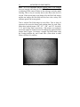
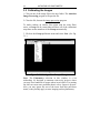
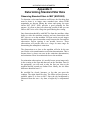
images later.) Figure 2-18 shows a sample Flat Field taken using
the evening twilight sky and I band filter. (Flats taken in other
filters will look very similar.)
Figure 2-18. Sample I Filter Sky Flat.
AUTOSTAR CCD PHOTOMETRY
17
3. Raw Data Reduction
This is the stage where the photometric data is extracted from the
images. When getting the data from an image, the data will be
automatically logged into a text file called ImageInfo.txt. The
software does a great deal of the work automatically.
3.1 Arranging the Files
The following procedure steps are just suggestions, and you can
develop your own scheme, as long as it makes sense and works for
you. (Windows software is notorious for putting files in places you
do not expect, and thus losing them for you. Experiment to make
sure the files are stored where you want them.)
Create a folder with the star name and observation double date in
the title, (e.g., TOri 22-23 Jan 07). Create separate folders for the
data from each filter (e.g., B Raw Data, V Raw Data, R Raw Data,
and I Raw Data). Put the stacked Flat Field image file for each
filter in the corresponding filter data folder. Do not worry about
the Dark Fields. These have already been subtracted on the fly
during imaging.
To simplify finding the proper image files, you can first open an
image file directly -- this will open the AutoStar Image
Processing application, then the image file. You should then close
the image file, but not the image processing program. This is done
to make sure the ImageInfo.txt file is created in the correct folder
by the software. Then you may open the specific image file you
wish to start with.
Note: You can open the ImageInfo.txt file at any time, to check
the log, using the NotePad program included with Windows. You
can also edit the log at any time and save changes. However, do
not change the name or location of the file until all the data has
been logged in. Experiment some with the following procedures,
until you are familiar with the process and how it works. It is very
important to know where the ImageInfo.txt file is stored, as this is
where your photometric data is located.
18
AUTOSTAR CCD PHOTOMETRY
3.2 Calibrating the Images
1. Click on one of the image files in the new folder. The AutoStar
Image Processing program will open the file.
2. Close the file, but not the image processing program.
To make working on similar files (taken with the same filter)
easier, a Group can be created that will have all of the calibration
steps done on the members of the Group automatically.
3. Click on the Group pull-down menu and select New. (See Fig.
3-1.)
Figure 3-1. Selecting a New Group of Images.
Note: The Photometry selection in this window is a bit
misleading. It's designed to automate time-series projects where
you may have hundreds of images taken in each filter. For starting
out, this can cause more problems than it solves. Ignore it for now.
Also, you may ignore the rest of the items from this pull-down
menu, as they mainly apply to astro imaging and not photometry.
AUTOSTAR CCD PHOTOMETRY
19
4. Select all the images of a given filter (e.g., the V filter images in
the V Raw Data folder). (See Fig. 3-2.)
Figure 3-2. Selecting Filter Files to Calibrate with Flat Field.
Note: This will create a new text file called ImageGroup.lst. Do
not move or rename this file. This is not a text file and cannot be
opened. Just let it be, as it defines the files in the Group.
5. From the Group pull-down menu, select Calibrate. (Fig. 3-3.)
Figure 3-3. Calibrate Selection.
20
AUTOSTAR CCD PHOTOMETRY
6. A Calibrate window will be displayed (Fig. 3-4) where you can
select and include a Bias, Dark Frame, and a Flat field image. If
you have used the Auto Dark Subtraction option while taking
images, or if the exposure time is less than 1 second, you do not
need to use another dark frame. If you have used a dark frame
when taking the images, the Bias image is not needed.
Figure 3-4. Calibrate Window.
Note: This will create a new file called NewImageGroup.lst. Do
not move or rename this file. This is not a text file and cannot be
opened. Just let it be, as it defines the Calibration for the files in
the Group.
7. Select the Flat Field you wish to use to calibrate with (e.g.,
click on Select Flat Field and find the flat field for the filter used
for the images to be calibrated – for instance, FV for the V filter
images). Click the Include Flat Field box, and if desired the
Include Bias button (after selecting the Bias image). Remember
that the Dark Frames have already been used on the fly when the
images were exposed (if the Auto Dark Subtract option was
selected). Also, the Bias Frame data is included as part of the
Dark Frame. Click on OK.
8. The program will now automatically calibrate all the images and
save the newly-calibrated images with new names (e.g.,
Calibrated_"file name"). The original (uncalibrated) images will
be left untouched. (See Fig. 3-5.)
AUTOSTAR CCD PHOTOMETRY
21
Figure 3-5. New Calibrated Image Files.
9. To organize the calibrated files, make a new folder within the
current folder. Call this folder “Cal Filter Name Data” (or “Cal
V” for the V filter calibrated images).
10. Repeat steps 3 through 9 for each of the other filters. You now
have sets of calibrated data ready to have the star magnitudes
determined.
3.3 Differential Magnitudes
The best and most accurate way to do photometry is to use
differential photometry, in which Program star magnitudes are
compared against known Comparison star magnitudes and then
normalized to produce a differential magnitude. This means you
must know the Comparison star Reference magnitude accurately
for each filter band.
3.3.1 Setting the Reference Magnitude
1. From within the Autostar Image Processing program, select File
and Open.
2. From within the Cal V folder (e.g., the Calibrated V filter
images) select the first image to be processed. Make sure the file
name has “Calibrated” in front of it.
22
AUTOSTAR CCD PHOTOMETRY
Note: AutoStar automatically adjusts the monitor display contrast;
so even if the images look faint, the data should be okay. If the star
image is too faint to be easily seen, you can adjust the contrast
manually. The adjustment only affects the display. You can also
expand the image to full screen if it helps.
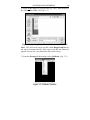
3. Start by drawing a small box around the Comparison star. There
will be a diagonal line across the (inner) box. The box should be
placed so that the line is approximately across the middle of the
star image. This is not very critical, as the software will find the
center of the star (the “centroid”). (See Fig. 3-6.) The direction
used to draw the box is up to you.
Figure 3-6. Photometry Cursor.
Note: The Photometry region cursor has three main components
(Fig. 3-6):
(a) Magnitude/Centroid Area
(b) Pixel List Area
(c) Profile Line
The Magnitude/Centroid rectangle bounds the entire area used in
the magnitude and/or centroiding calculations. This is a bit
confusing – to properly determine the magnitude of a star, only
draw the small box (shown to the lower left – the Pixel List Area)
around the star of interest. The Profile line delineates the pixels
that will be displayed when the Draw Profile function is selected.
AUTOSTAR CCD PHOTOMETRY
23
You will see the term “centroid” appear many times when reading
about CCD photometry. This is a bit of software “magic”. The
centroid of a star image is essentially its center of gravity or center
of brightness. The CCD software can find this center very
precisely. This is important, because when selecting the star for
processing, you do not need to select it exactly. Just as long as you
are close, the software will find the center (centroid) of the star and
reference everything about the star relative to that center. This is
also important when using the CCD camera for tracking, as the star
image center can be determined precisely.
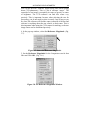
4. In the pop-up window, select Set Reference Magnitude. (Fig.
3-7).
Figure 3-7. Select Set Reference Magnitude.
5. Set the Reference Magnitude for the Comparison star for that
filter and Click OK.. (Fig. 3-8.)
Figure 3-8. Set Reference Magnitude Window.
24
AUTOSTAR CCD PHOTOMETRY
Note: This will set the Reference magnitude for the Comparison
star. This action must be performed with each image. The other
star measurements will now produce magnitude values referenced
to the Comparison star Reference magnitude that was entered. This
will create a new text file in the folder called ImageInfo.txt. All
the data that is acquired from the images will be logged into that
file. Do not move or rename the file until all of the data (for all the
filters) has been entered.
3.3.2 Aperture Diameter, Annulus, and
Centering Box Size Settings
The Aperture Diameter, Annulus, and Centering Box Size can
be changed, but unless you want to experiment or know what you
re doing, it is best to leave these values at their default settings of
8, 15, and 15, respectively.
3.3.3 Raw Magnitude Determination
6. Draw a box around the first Program star. A widow will pop up.
Select Determine Magnitude. (Fig. 3-9.)
Figure 3-9 . Select Determine Magnitude.
7. A Magnitude Determination window will be displayed,
indicating the selected Program star magnitude referenced to the
Comparison star, along with other data. (Fig. 3-10.)
AUTOSTAR CCD PHOTOMETRY
25
Figure 3-10. Magnitude Determination Window.
8. Click on OK. Do not click on “Log”, as the data will be logged
twice. Just click OK.
9. Repeat Steps 1 - 8 for each Program star you wish to know the
magnitude of.
10. As a double-check and a way to indicate where you are in the
Log file, determine the magnitude of the Comparison star as the
last measurement. It should be the same as what was set earlier for
the Reference magnitude.
Note: To continue with additional images taken with the same
filter, repeat Steps 1 - 8; but you will not need to re-enter the
Reference magnitude value as it is already set (for that filter), so
just click OK for that step. You will need to use the Set Reference
Magnitude with each image, however.
11. When done, you should have data from all the images for the
given filter. You should also have a single text file called
“ImageInfo.” You now can rename the text file. Call it
“V Data.txt” (for the V filter images.)
26
AUTOSTAR CCD PHOTOMETRY
12. Repeat Steps 1 - 11 for the other filter images. A text log file
called ImageInfo.txt will be created.
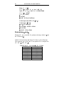
3.4 ImageInfo File
The ImageInfo.txt file is a text file that is automatically created
when determining the magnitudes of the stars. Table 3-1 shows a
screen shot of a sample file.
Table 3-1. ImageInfo Log Text File Example.
The X and Y Center data helps identify which star the data applies
to. Regarding the rest of the data: the Magnitude, which is
relative to the Reference Magnitude, Flux, and Max are the data of
most interest. The FWHM (Full Width Half Maximum) number
gives an idea of the shape of the star image. If this gets too far
away from approximately 6, there may be a problem with the data.
The rest of the data may be of interest for determining the quality
of the data.
AUTOSTAR CCD PHOTOMETRY
27
4. Additional Data Reduction
The raw magnitude data now must be used to calculate the average
magnitudes and data spread or standard deviations, in addition to
calculating the Air Mass and Heliocentric Julian Date (HJD). A
Mean time for the set of exposures is also calculated. There are
various ways to do this, but since it is time-consuming, it is best to
use a computer program. A spreadsheet program can be used (such
as Microsoft Excel™), but a much better way is to use a database
program such as FileMaker Pro™. Since you will be dealing with
a vast amount of data, it is worthwhile learning to use a program
like FileMaker Pro so you can develop and customize your
database programs as needed.
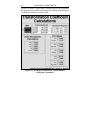
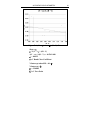
4.1 DATABASE PROGRAM
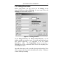
The following example database was developed with FileMaker
Pro at HPO. Figure 4-1 shows a screen shot of one of the layouts
of the FileMaker Pro program. This one is designed specifically for
Theta 1 Orionis data (an interesting eclipsing binary star in the
Trapezium in Orion). The white data fields are data entry fields
and the colored (shaded) fields are auto entry and calculated data.
Figure 4-1. FileMaker Pro Data Summation Program.
28
AUTOSTAR CCD PHOTOMETRY
This program was created quickly and saves a great deal of work
when summarizing the data. The white data fields are data entry
fields and the green and black shaded entries are calculated data
fields. Data fields have been created for up to 4 program stars.
Data fields shaded in blue are global fields used for all the records.
The RA and Dec star position values are used in determining the
Air Mass and HJD (Heliocentric Julian Date). Since the stars in
this project are all located close together in the image, only one
star’s RA and Dec need be used.
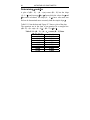
4.2 DATA LIST
A summary list of the data can be easily generated and displayed
or printed. Data can be found by any field or combination and
sorted in various ways. Figure 4-2 is a screen shot of a report
layout in the FileMaker Pro program.
Figure 4-2. Database List of Data Records.
AUTOSTAR CCD PHOTOMETRY
29
5. Advanced Data Reduction
5.1 Reducing the Raw Magnitudes to Standard
Magnitudes
So far all or our work has produced raw (instrumental) magnitudes
that are unique to the equipment used to produce them. Raw
magnitudes are fine, if you are only interested in changes. Many
times, data may be desired to be combined with data taken with
other equipment. Calibrating the data to a standard will allow it to
be useful. Once calibrated, your data will represent true
magnitudes. To do this, the raw magnitudes must be corrected with
color transformation coefficients. See Appendixes C and D for the
details on determining these coefficients.
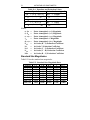
5.2 Transformation Coefficient Equations
(R – I) = γ *(r – i) – k'ri * X + ζri
(V – I) = α *(v – i) – k'vi * X + ζvi
(V –R) = β *(v – r) – k'vr * X+ ζvr
V = v +ε * (B – V) – k'v * X + ζv
(B – V) = μ * (b – v) – k'bv * X + ζbv
Where:
Instrumental Magnitudes
Instrumental Magnitude = –2.5 * log10 (Star Counts)
i
v
r
b
Corrected Magnitudes
I
V
R
B
(V – I)
(R – I)
(V – R)
(B – V)
Transformation Coefficients (Must be determined)
α for (V – I)
ε for V
β for (V – R)
μ for (B – V)
γ for (R – I)
30
AUTOSTAR CCD PHOTOMETRY
Extinction Coefficients
(Not needed for differential photometry)
k'vi for (v – i)
k'v for v
k'vr for (v – r)
k'bv for (b – v)
k'ri for (r – i)
Zero Points
(Not needed for differential photometry)
ζvi for (V – I)
ζv for V
ζri for (R – I)
ζbv for (B – V)
Note: While Extinction and Zero Points are not needed for
differential photometry, they are needed to determine the color
transformation coefficients.
The equations for CCD Differential Photometry then simplify to
the following:
(R – I) = γ * (r – i)
V = v + ε * (B – V)
(V – I) = α * (v – i)
(B – V) = μ * (b – v)
(V – R) = β * (v – r)
Once the color transformation coefficients have been determined,
they can be used along with the raw magnitudes to produce
corrected magnitudes.
AUTOSTAR CCD PHOTOMETRY
31
APPENDIXES
A. Modifying the DSI Pro Camera
33
B. Calculating the Air Mass
45
C. Determining Standard Star Data
55
D. Determining BVRI Extinction Coefficients
59
E. Determining BVRI Color Coefficients
67
F. Least Squares Method
85
G. FITS Header
89
H. Light Box Design and Construction
91
I. Suggested Projects
99
J. References
103
INDEX
107
32
NOTES
AUTOSTAR CCD PHOTOMETRY
AUTOSTAR CCD PHOTOMETRY
33
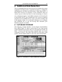
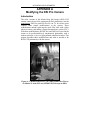
APPENDIX A
Modifying the DSI Pro Camera
Introduction
The color versions of the Meade Deep Sky Imager (DSI) CCD
camera cannot be used for astronomical filter photometry, but the
monochrome DSI Pro (and DSI Pro-II) can. To do serious work
requires some simple modifications to the camera. These
modifications include replacing the stock filter slide with a filter
wheel (or turret), and adding a simple thermoelectric cooler (TEC).
With these modifications, the DSI Pro (and DSI Pro-II) provide the
means to do professional-level astronomical photometry with a
modest telescope, even in a light-polluted suburban location. This
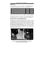
chapter describes these modifications and what is needed to do
BVRI CCD photometry with the camera.
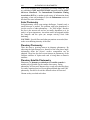
Figure A-1. Modified DSI Pro CCD Camera and Filter Turret
on Meade 12 inch (30.5 cm) LX200 GPS Telescope at HPO.
34
AUTOSTAR CCD PHOTOMETRY
The Affordable Meade Deep Sky Imager (DSI)
While CCD cameras for astronomical use have been around for
more than a decade, it has only been recently that affordable and
easy-to-use CCD devices have been made available to the amateur
market. Some of the first of these were digital web cams. Some
folks figured them out and made modifications that produced
surprisingly high-quality results. But web cams work best on the
brighter objects such as the planets, the Moon, and solar imaging.
For deep-sky imaging, the web cams need to be modified, but
these modifications are beyond the capability of many amateurs.
When Meade introduced the color Deep Sky Imager (DSI), that
changed. Now one could do deep-sky imaging of faint objects
without needing to make complicated modifications to the camera.
In addition, the AutoStar Suite software that comes with the DSI
series is excellent. It’s worth the price of the camera alone.
Learning the software requires some dedication, as the quality of
the software far exceeds the documentation (thus, this book!)
However, two technical issues prevent use of the color versions of
the DSI camera for effective astronomical filter photometry.
Because the Sony HAD EX-View® color CCD chip used in the
DSI color version has built-in microlens red-green-blue (RGB)
filters on the photosites, it would be hard or impossible to find
proper filters to match the camera to the standard photometric
system. The other issue, while mainly a problem only during the
warmer months, is that the DSI camera is electrically uncooled and
operates at ambient temperature.
Monochrome Deep Sky Imager Pro (DSI Pro)
Shortly after the color DSI was released, Meade introduced a
monochrome version, the DSI Pro. The monochrome DSI Pro and
the newer DSI Pro-II cameras provide a good starting point for
serious CCD photometry at moderate expense. Because these
cameras use a monochrome version of the Sony CCD chips, a fourposition filter slide for RGB filters is included, for tri-color
imaging (plus a “clear” or IR blocking filter).
AUTOSTAR CCD PHOTOMETRY
35
The set of standard RGB astro imaging filters is provided at extra
charge. The advantages of using the DSI Pro with the external
filters are that the monochrome camera is more sensitive, and
provides better resolution, as well as allowing use of different
filters.
While the included filter slide could be used to hold photometric
filters, it quickly becomes apparent that is not a good idea. The
specialized BVRI photometric filters are expensive, and the filter
slide is of open construction, exposing the filters to dust, dew,
fingerprints, and scratches. A filter wheel (turret) is a much better
way to hold and protect the filters.
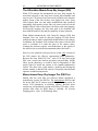
Adding a Filter Wheel – Installing the Nose Piece
Adapter
The first step in readying the DSI Pro for photometry is to replace
the stock filter slide holder with a low-profile adapter plate similar
to that used on the color DSI (see Figure A-2). This gets rid of the
large openings where the slide goes and also reduces the distance
from the filters to the CCD chip. The adapter is threaded for
standard TEE thread accessories. In the U.S. this adapter plate can
be purchased for about $40 from ScopeStuff. (See the list of
suppliers at the end of this Appendix.)
Note: The original standard TEE threaded to 1.25 inch (31.7 mm)
nose piece can also be used with the new adapter, but it's better to
mount the filter wheel closer to the camera than allowed by the
nose piece. The filter wheel we describe comes with TEE thread
couplers for the purpose.
Replacing the original filter slide holder adapter with the lowprofile adapter plate is very simple. There are four small Phillipshead screws that hold the adapter in place. Those screws and the
original adapter are removed and replaced with the low-profile
adapter using new shorter screws (provided).
36
AUTOSTAR CCD PHOTOMETRY
Note: There are four hex-head screws at the corners of the camera.
The hex-head screws hold the camera together. Do not remove
those screws for this modification.
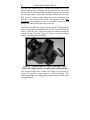
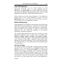
Figure A-2. DSI Pro Camera with Filter Slide (left)
and Low-Profile and Original Nosepiece Adapters (Right).
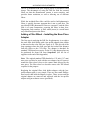
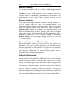
Filter Wheel
With the low-profile nosepiece adapter installed on the DSI Pro,
the next step is to add a filter wheel. There are several available on
the market, ranging from under $100 to over $1,000. An excellent
and inexpensive choice is the ATIK Manual Filter Wheel. This can
also be purchased from ScopeStuff or from Adirondack Astro
Video (the U.S. importer) for about $200. The ATIK filter wheel is
well-made and can hold up to five standard 1.25 inch (31.7 mm)
screw-in filters. Figure A-3 shows the ATIK Filter Wheel
disassembled and the filter carrier disk with photometric filters
installed. The ATIK wheel uses standard TEE threaded adapters
(provided) to attach it to the low-profile nose piece on the camera.
It also comes with a removable standard 1-1/4 inch (31.7 mm) to
TEE thread nose piece.
Since the U band filter is not used with the DSI CCD camera, an
optional filter such as Hydrogen Alpha could be placed in the fifth
position, or the “Clear” (IR Block) filter that comes with the DSI
camera can be installed, for occasional regular deep-sky imaging
or “white light” photometry.
AUTOSTAR CCD PHOTOMETRY
37
Figure A-3. Disassembled ATIK Filter Wheel.
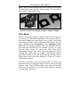
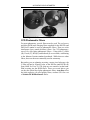
CCD Photometric Filters
For most photometry, special filters must be used. The red, green,
and blue (RGB) astro imaging filters supplied for the DSI Pro and
DSI Pro-II cannot be used as photometric filters. These are color
interference layer coated (dichroic) filters. For CCD photometry,
sets of five dyed glass photometric filters – Ultraviolet (U), Blue
(B), Visual (V), Red (R), and Infrared (I) are available, conforming
to the Johnson-Cousins standard passbands.. While there are other
filters, these are the most commonly used in astronomy.
But unless you are planning on using a meter-sized telescope, the
U filter will not be of much value, as the DSI Pro (and DSI Pro-II)
Sony HAD Ex-View™ CCD chips are not sensitive in that band.
Plan on using just the BVRI filters. There are several places you
can buy the special dyed glass photometric filters. Astrodon offers
the least expensive yet good quality filters, at about $310 for a set
of Schuler BVRI Photometric filters.
38
AUTOSTAR CCD PHOTOMETRY
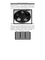
Figure A-4 shows the ATIK filter wheel disk with BVRI filters
installed in positions 1, 2, 3, and 4, respectively. Position 5 could
be used for a U filter, but because the CCD camera chip is
insensitive in that band, the Meade IR blocking (“Clear”) filter is
used, for deep sky imaging or “white light” photometry.
Figure A-4. Filter Wheel Disk with BVRI Photometric Filters.
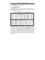
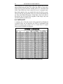
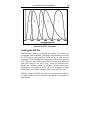
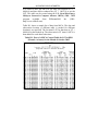
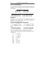
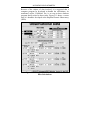
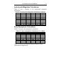
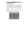
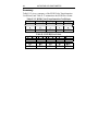
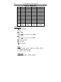
Table A-1 lists the standard UBVRI Johnson-Cousins system filter
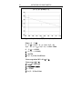
bandwidths, measured at the half-height point. Figure A-5 shows
the standard UBVRI filter passbands, plotted in Ångstroms. (10
Ångstroms = 1 nanometer.) Note: U band work is not practical
with most amateur CCDs and is only noted for reference here.
Table A-1. UBVRI Filter Bandwidths.
Band
Center
Width
367 nm
66 nm
U
436 nm
94 nm
B
545 nm
88 nm
V
638 nm
138 nm
R
797 nm
149 nm
I
Bandwidths measured at half-height point.
AUTOSTAR CCD PHOTOMETRY
39
Figure A-5. Standard UBVRI Johnson-Cousins
Photometry Filter Passbands.
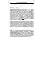
Cooling the DSI Pro
The DSI series cameras use ambient air cooling. The camera case
is equipped with an internal “cold finger” that transmits heat from
the CCD chip to the backplate, which acts as an efficient heat
exchanger. With cool night time temperatures, these units perform
well. However, Dark Frames must still be created and subtracted
from each image to get rid of “hot” pixels and thermal noise.
During the summer months in Phoenix, Arizona observatory
temperatures can approach 100°F (38°C) at midnight. At those
temperatures, even subtracting dark frames does not work well.
Adding cooling to the DSI Pro started as an experiment at HPO to
see what could be done at minimum cost and the least amount of
modification.
40
AUTOSTAR CCD PHOTOMETRY
This cooling modification can be used on all the DSI series
cameras. In addition to reducing dark current, electronic cooling
increases the camera's sensitivity.
TEC Cooler Mods
Perhaps the most effective way to cool the CCD is by using a
Peltier Junction Thermoelectric Cooler (TEC). Peltier Junction
TECs are fascinating devices. They consist of a sandwich of
semiconductors connected in parallel, between two metallic plates.
By applying a DC voltage across the device, one plate gets hot
while the other one is cooled. The amount of heat and cooling
produced can actually be surprising! Care must be taken when
experimenting so that the unit doesn’t overheat. Attaching a finned
heatsink and a fan is very important on the hot side. Thermal
grease needs to be applied on both plate surfaces to provide
effective transfer of the heat (and cooling).
Some will note that there is no temperature regulation or sensor
included in our mod. These features could be added, but would
increase the complexity. The lack of temperature regulation has
not been a problem at HPO. If the camera is allowed to run with
power and cooling ON for 15 to 30 minutes, the temperature will
stabilize. The exact temperature is not important. Once the unit has
stabilized, new dark frames for that evening should be taken. This
procedure works well.
Note: The modifications described here involve opening the
camera case to install the equipment, and probably will void the
camera warranty. Some experience with electronics or kit
building is highly recommended. A bolt-on TEC cooler backplate
assembly is available commercially. A simple clip-on 12VDC
electric fan is also available as a standard accessory from Meade,
which will lower the camera temperature about 9°F (5°C).
AUTOSTAR CCD PHOTOMETRY
41
Parts List
The following List of Parts, available from All Electronics is
recommended. (Catalog prices listed are as of Spring 2007):
Part Name
40 mm 12VDC Thermo Electric Cooler
Heat Sink with 12 VDC Fan
12 VDC, 3.5A Power Supply
Tube of Thermal Grease
P/N
PJT-7
CF-215
PS-1231
TG-20
Price
$14.75
$7.50
$15.85
$4.25
You will also need several 6-32 x 1 inch nylon (non-conducting)
screws, some wire, and a power connector. You can get the
miscellaneous parts at a local store such as Radio Shack for a
couple of dollars. Total cost for the electronic parts is under $50.
DSI Pro TEC Cooler Modifications
Modifications to the DSI Pro camera require opening the camera
and drilling holes through the back of the case for two 6-32 screws
(for added stability, 4 screws could be used) to hold the TEC/Heat
Sink and Fan assembly against the back of the DSI case. Note:
This will void the camera warranty. Use a 2.5 mm Allen wrench
and carefully open the camera from the front by removing the hexhead screws in the corners. Be careful not to tear or stretch the
rubber gasket (see Figure A-6).
Figure A-6. Views Inside the DSI Pro with Cold Finger
(White Square) and Nylon Mounting Screws Shown.
Circuit Board and Gasket Below.
42
AUTOSTAR CCD PHOTOMETRY
Now place the center of the TEC (against the camera back) so it is
directly opposite the cold finger (on the inside of the case). Drill
and tap 2 (or 4) matching holes through the camera case and into
the heat sink. Make sure the hole spacing is sufficient to clear the
TEC. Use two nylon (or non-conductive) screws to hold the heat
sink/TEC to the back of the camera. The purpose of the nonconducting nylon (plastic) screws is to reduce or prevent heat
transfer from the hot heat sink back to the case.
Carefully reassemble the camera, without tearing or damaging the
rubber sealing gasket, and tighten the four hex head screws on the
front to close the case. Add some foam for insulation around the
camera to keep it cool. See Figure A-7 for a view of the modified
camera with foam insulation added.
Figure A-7. Modified DSI Pro with Focal Reducer, Filter
Wheel, TEC/Heat Sink/Fan Assembly and Foam Insulation.
The optional Meade Series 4000 Focal Reducer lens shown in
Figure A-7 provides a larger field of view for the imager. This
makes finding the stars and getting comparison stars in the same
view much easier.
AUTOSTAR CCD PHOTOMETRY
43
Wiring and Schematics
The polarity of the TEC is a bit ambiguous, but you can’t damage
it by reversing the connections. After connecting the power supply,
check to verify which side gets “hot” and place that side against
the finned heat sink (away from the camera back). Don't forget to
apply ample thermal grease between the TEC plates and the
camera back, and also to the finned heatsink.
A 12VDC fan is installed on the back of the heatsink, to draw
additional cooling air through the fins. At HPO, a 3.5 A 12VDC
supply was used, separate from the telescope power, operating
from 110VAC. For a portable setup, a 12VDC battery supply
could be used. A power indicator light, an ON-OFF switch, and a
fuse could be added, or the power supply can simply be unplugged
when the camera is not in use (as shown in the illustrations).
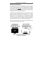
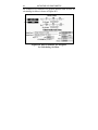
Figure A-8 shows drawings of the mechanical modification and an
electrical wiring schematic, respectively.
Figure A-8. Mechanical Modification Drawing
and Electrical Schematic.
44
AUTOSTAR CCD PHOTOMETRY
Conclusion
With the addition of BVRI photometric filters and a few simple
modifications, the monochrome DSI Pro and DSI Pro-II CCD
cameras can be used for serious astronomical photometry. Beware,
photometry can be addictive, but very rewarding.
List Of Suppliers for Filters and Cooler Mods
(Note: This list is provided for information only.)
Low-Profile Nose Piece TEE Thread Adapter, from Scope Stuff:
http://www.scopestuff.com/ss_dsif.htm
ATIK Filter Wheel, from Adirondack Astro Video:
http://www.astrovid.com/prod_details.php?pid=2680
ATIK Products web pages:
http://www.telescope-service.com/atik/start/atikstart.html
Schuler BVRI Photometric Filters from Astrodon:
http://www.astrodon.com/products/product.cfm?CatID=4
(Note: The U band filter is not needed for CCD work.)
TEC Cooler, Heat Sink, and Fan, and other electronic parts from
ALL Electronics: http://www.allelectronics.com/
Optional Accessories
Outback TEC Cooler (Bolt-on replacement back plate assembly
with TEC cooler, heatsink./fan, and temperature controller) from
Steven Mogg (Australia): http://webcaddy.com.au/Outback
Clip-On 12VDC Fan Accessory Part No. 04531 from
Meade Instruments (See Meade dealers):
http://www.meade.com/dsi/dsi_accessories.html
Series 4000 Focal Reducer Lens from Meade Instruments
(See Meade dealers).
_____________
Note: All of the modifications described in this Appendix are
performed at the sole risk of the owner. No fitness or suitability of
use is implied, and may void the camera warranty. All
consequences are at the sole risk of the owner/installer.
AUTOSTAR CCD PHOTOMETRY
45
APPENDIX B
Calculating the Air Mass
Introduction
The listed corrected magnitudes of stars are given as they would be
seen outside the Earth's atmosphere. These values are the values
found in books and tables that list a star's extraterrestrial
magnitude.
When starlight passes through the Earth's atmosphere, it is
diminished by a variable factor. This attenuation, known as
atmospheric extinction, is caused by absorption of some of the
starlight by the atmosphere. The greater the thickness of the
atmosphere the starlight passes through, the greater the extinction.
Observations made at observatories located at high altitude have
less extinction than those at a lower altitude. This is one reason
why most major observatories are located on mountain tops.
Observations made directly overhead at the Zenith have the least
extinction for a given location. The extinction increases as a star is
viewed further from the Zenith, and is at a maximum at (or below)
the horizon. The section of atmosphere that the starlight travels
through is known as the Air Mass.
One of the first steps in determining a star's magnitude from
measurements taken at the Earth's surface is to know the
extinction. The key factor in knowing the extinction is in knowing
the star's air mass at the time of the observation.
The following is an explanation of how to determine air mass for a
given location, time, and star position. While seemingly simple,
there are many pitfalls in determining the air mass.
46
AUTOSTAR CCD PHOTOMETRY
Getting Started
A star's Air Mass, X, is the effective path length of air through
which starlight has passed to reach the observer. By definition,
X = 1.00 at the Zenith (straight overhead) and increases as one
observes stars closer to the horizon. Letting Z be the angular
distance of a star from the Zenith (0° ≤ Z ≤ 90°), then the simplest
relationship is:
X = sec Z
This would be correct if the Earth and its atmosphere were flat.
However, the Earth's curvature causes the relationship to
overestimate the air mass for large zenith distances. The correct
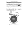
configuration is illustrated in Figure B-1.
Atmospheric
Distances
c>b>a
a
+
Air Mass c
is much greater
than Air Mass a
Zenith
b
c
+
a
b
c
Horizon
+
Earth
Atmosphere
Figure B-1. Illustration of a Star's Air Mass
(Accounting for Curvature of the Earth’s Atmosphere).
AUTOSTAR CCD PHOTOMETRY
47
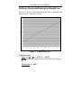
Two equations are in common use that take into account not only
the curvature, but also the refraction, of the Earth’s atmosphere:
X = secZ (1 – 0.0012 (sec2Z – 1))
X = secZ – 0.0018167 (secZ – 1 ) - 0.002875 (secZ – 1)2
– 0.0008083 (secZ - 1)3
Where: The value of secZ depends only on the location of the
observer and the position of the star in the sky and can be
determined by:
secZ = (sinLAT sinδ + cos LAT cosδ cosHA)-1
In this equation , LAT is the observer's latitude while δ and HA
are the star's Declination and Hour Angle, respectively. All values
are given in decimal degrees.
Note: Z in the first equation above refers to the apparent zenith
distance of a star (i.e., taking into account atmospheric refraction).
In physical terms, this distance is equivalent to the angle between
the optical axis of a telescope and a plumb bob hanging from the
mounting. However, direct determination of this angle is both
cumbersome and inherently inaccurate. In contrast, Z in more
complex equations refers to the true Zenith Distance, which
assumes that no atmospheric refraction is present. Use of the latter
value is preferred, as it can be readily calculated from available
parameters.
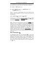
Star's Declination (δ)
As illustrated in Figure B-2, the Declination, δ, of a star is the
angular distance above or below the celestial equator (which is the
projection of the Earth's equator on the celestial sphere). The
declination of a star on the celestial equator is 0°, while that of a
star at the North Celestial Pole (NCP) would be +90°. Stars
between the celestial equator and the NCP have declinations of
0° ≤ δ ≤ +90°.
48
AUTOSTAR CCD PHOTOMETRY
Similarly, a star situated at the South Celestial Pole (SCP) would
have δ = –90°, while those between that pole and the celestial
equator have declinations of –90° ≤ δ ≤ 0°.
NCP
+
o
+30
o
o
Eq
ua
to
r
+90
0
-30
o+
o
-90
C
0
el
es
tri
a
l
Earth
o
SCP
Figure B-2. Illustration of a Star's Declination.
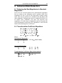
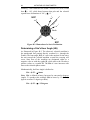
Determining a Star's Hour Angle (HA)
As illustrated in Figure B-3, The observer's celestial meridian is
the north-south line passing directly overhead (i.e., through the
Zenith). The hour angle, HA, of a star is the amount of time since
the star crossed the celestial meridian or until the crossing will
occur. Stars East of the meridian are designated either as a
negative value or with the symbol E, while stars to the West have
positive values or a symbol W. The HA of a star increases with
time as the celestial sphere rotates.
Mathematically, the Hour Angle is defined as:
HA = (LST – α) hours
Note: HA is defined in hours, but must be converted to degrees
(angle). To produce this, multiply HA in hours by 15 (the sky
appears to rotate 15 degrees per hour).
HA = (LST – α) * 15 degrees
AUTOSTAR CCD PHOTOMETRY
49
Where: LST is the local sidereal time and α is the star's Right
Ascension. The LST is simply the Right Ascension of a star on the
observer's celestial meridian at the time of the observation.
+
0 hr
+
East
Observer's Meridian
(North -South Line)
1.5 hr
+
West
3 hr
Observer's Southern Horizon
Figure B-3. Illustration of Star's Hour Angle for Northern
Hemisphere Observers Facing The Southern Horizon.
Note: The star on the meridian may or may not be the star being
observed, and is referred to only to define LST.
Determining Local Sidereal Time (LST)
The LST can be calculated; however high accuracy is needed to
determine an accurate LST. Most computers and computer
programs have a difficulty in providing sufficient accuracy.
Another approach is to look up the Greenwich Mean Sidereal Time
(GMST) from an Astronomical Almanac for UT = 00:00:00
(GMS0hUT), subtract (if West of Greenwich) or add (if East of
Greenwich) the observation longitude (in hours) and then add the
UT of the observation times the factor 1.00274:
LST = (GMS0hUT – Long + 1.00274 * UT)
50
AUTOSTAR CCD PHOTOMETRY
Where:
GMS0hUT is Greenwich Mean Sidereal Time at UT = 00:00:00.
Long is the Longitude of the observer’s site converted from
degrees to time from GMT.
UT is the Universal Time of the observation.
The factor 1.00274 is to convert UT solar time to UT sidereal time.
Note: Convert all times to decimal hours:
(Hours + minutes/60 + seconds/3600).
For example:
Kitt Peak National Observatory has a (geodetic) longitude of:
–111° 35m 52s or –111.59777778 degrees. This is equivalent to:
–7h 26m 23s or 7.423555556 hours West from Greenwich.
Long. (degrees) = 111.597777778 (degrees) * 24/360 (hrs/degree)
Long. (time) = 7.423555556 hours
If an observation was made at 4h 24m 16s (4.406154 hours) UT on
09 September 1990,
GMS0hUT = 23h 11m 52s or 23.18555556 hours
UT = 4.406154 hours
Thus:
LST = 23.18555556 – 7.423555556 + (1.00274 * 4.406154)
LST = 20.180227 hours
Creating an LST Table Using MICA Software
If one is to use a computer program to calculate this, it may be
desirable to create a look-up table of all values of LST at UT =
00:00:00 for a ranges of dates. While individual observation UTs
can be entered and LST determined, it is not practical to create a
table of such times.
AUTOSTAR CCD PHOTOMETRY
51
It is better to have just one LST per date and location at UT =
00:00:00 and then add or subtract the (UT * 1.00274) to get the
LST. This table can be created using the U.S. Naval Observatory
Multiyear Interactive Computer Almanac (MICA) 1800 - 2050
program
available
from
Willmann-Bell,
Inc.
(URL:
http://www.willbell.com).
Table B-1 shows a sample list of data from MICA. The date and
observation location (a different table is needed for different
locations) are specified. The location's LST for that date at UT =
00:00:00 is then looked up. The observation's UT times 1.00274 is
then added for each observation time.
Table B-1. Part of a MICA Created Table for LST at HPO
(Phoenix, Arizona) for the Month of October 2005.
52
AUTOSTAR CCD PHOTOMETRY
LST Example
For 21 October 2005 at UT = 07h 10m 00s or 7.166667 hours.
Using the MICA printout shown in Table B-1, the Local Mean
Sidereal Time for 21 October 2005 for HPO (Phoenix , Arizona) at
Longitude = 112° 13m 22.0s West and Latitude 33° 30m 06.0s
North is 18h 29m 16.1843s or 18.487829 hours.
LST = 18.4897829 + 1.00274 * 7.1666667
LST = 25.674132 hours
Note: To test and adjust LST:
If (LST Lookup + UT * 1.00274) ≥ 24,
Use: (LST Lookup + UT * 1.00274) - 24
Otherwise, use: LST Lookup + UT * 1.00274.
Since the above value is greater than 24, 24 hours must be
subtracted from it to give:
LST = 1.674132 hours
Determining the Hour Angle (HA)
HA = LST – α
To determine the Observation's Hour Angle (HA), the observed
star's Right Ascension (α) is subtracted from the Local Sidereal
Time (LST).
For example:
Assume star α Aur:
RA = α = 5h 16m 41.3s or 5.278139 hours
Dec = δ = 45° 59m 53.0s or 45.998056 degrees
For LST = 1.674132 hours:
HA= 1.674132 – 5.278139
HA = –3.604007 hours
To convert HA from hours to degrees:
HA = –3.604007 * 15 degrees
HA = –54.060105 degrees
AUTOSTAR CCD PHOTOMETRY
53
Alternatively, the hour angle of a star can be determined directly
from the telescope's right ascension setting circle (if so equipped)
by noting the difference in right ascension between the star and the
meridian.
Because the celestial equator intersects the observer's horizon at
the due east and west points, a star with δ = 0° (on the celestial
equator) is above the horizon for exactly 12 hours; the star rises
with HA = –6 hour and sets with HA = +6 hours. For observers in
the Earth's northern hemisphere, a star with δ < 0° spends less than
12 hours above the horizon each day, while a star with δ > 0° is
visible more than 12 hours per day. As a final comment, note that
circumpolar stars never rise nor set, so that their hour angle can
range from –12 hours (12 hours East) to +12 hours (12 hours
West). The hour angle is zero for stars at upper culmination.
Determining the Air Mass
Now that we know the HA for the observation, the value of secZ
and thus the Air Mass, X, can be calculated:
secZ = (sinLat sinδ + cos Lat cosδ cosHA)
-1
Latitude for HPO (Phoenix, Arizona):
Lat = 33° 30m 06.0s North or +33.50166667 degrees
Declination and Right Ascension for α Aur:
δ = +45.998056 degrees
HA = –54.060105 degrees
Thus:
secZ = 1.4061942273781
To determine Air Mass, X:
X = secZ – 0.0018167 (secZ – 1) – 0.002875 (secZ – 1)2
– 0.0008083 (secZ – 1)3
X = 1.404928
54
AUTOSTAR CCD PHOTOMETRY
An example of a FileMaker Pro program printout used at HPO for
calculating Air Mass is shown in Figure B-4.
Figure B-4. HPO FileMaker Pro Program
for Calculating Air Mass.
AUTOSTAR CCD PHOTOMETRY
55
Appendix C
Determining Standard Star Data
Observing Standard Stars in M67 (NGC2682)
To determine color transformation coefficients, the first thing that
must be done is to image some standard stars whose BVRI
magnitudes are known. During the winter and spring, the open
cluster M67 (NGC 2682) provides a good grouping for this
purpose. It is best to plan your observing session so that you can
observe M67 twice over a long time period during the evening.
One observation should be with M67 far from the meridian, either
before or after the meridian crossing; and one observation with
M67 close to or on the meridian. For best results several images
should be taken spaced somewhat evenly between the first and last
observation. Precise spacing is not needed, however. These
observations will provide data over a large air mass range for
determining the atmospheric extinction.
The observation at or close to the meridian will also be the one
used for the color transformation coefficient determination. This is
because there is always an error in the extinction determination,
and extinction effects are minimized close to the meridian.
For wintertime observations, it is usually best to get an image early
in the evening to the East and then one on the meridian. Later in
the springtime, you will need to take the first one close to the
meridian and the second one further West. Ideally, the Air Mass
difference should at least 1.5.
Be watchful for clouds, hazeness, or fog that can upset the
readings. The night should be clear. The Moon will not present a
problem, unless it is close to M67. Since the sky background is
subtracted from the star + sky data, a bright sky is compensated
for.
56
AUTOSTAR CCD PHOTOMETRY
Figure C-1 shows a wide field view of M67, from the First
Palomar Sky Survey (POSS I). (Ref: R. Miles, JBAA 108 p. 65,
1998.) The smaller rectangle near the bottom is where the stars of
interest lie.
The epoch 2000 coordinates for star cluster M67 (NGC 2682) are:
RA = 08h 51m 21s , and Dec = +11d 46m 18s.
The epoch 2000 coordinates for the area of interest in M67 are:
RA = 08h 51m 44s, and Dec = +11d 46m 32s.
Figure C-1. M67 Open Cluster Photograph.
Figure C-2 is a composite of ten 4-second exposures using a B
filter and a modified DSI Pro CCD camera on a 12 inch (30.5 cm)
LX200 GPS telescope at HPO.
AUTOSTAR CCD PHOTOMETRY
57
Figure C-2. M67 CCD Image Taken at HPO.
Table C-1 shows sample raw ADU Total Flux counts for the
standard stars in M67. These data were taken with 15-second
exposures in each filter (sky counts have been subtracted by the
software).
Table C-1. Sample Raw ADU Total Flux Data from M67.
Star ID
B
M67-081 418581.7
M67-108 162246.7
M67-117 16926.3
M67-124 32157.9
M67-127
7160.0
M67-130 16492.3
M67-134 27774.8
M67-135 38165.5
Filter
V
R
672151.8
550120.0
816575.1 1321557.5
816575.1
66663.2
80115.8
83593.1
43625.1
50523.8
42037.1
44009.5
73617.1
84096.3
154767.1
212966.4
I
183962.9
839716.2
33397.6
35806.7
22592.5
18563.3
39921.9
117236.9
Figure C-3 shows the star locations used in M67. Use the
identified stars along with Table C-2 for their standard magnitudes.
58
AUTOSTAR CCD PHOTOMETRY
Figure C-3. M67 Finder Chart for Star Identifications.
BVRI Standard Magnitudes in M67
Table C-2 lists the BVRI standard magnitudes of the stars in M67
to be used for the calibration.
Table C-2. M67 BVRI Standard Magnitudes.
Star
081
108
117
124
127
130
134
135
B
V
B–V
R
V–R
I
R–I
V–I
9.944
10.024 –0.080 10.064 –0.040
10.092
–0.028
–0.068
11.081
9.711
1.370 10.064
0.707
8.360
0.644
1.351
13.409
12.625
0.784 12.159
0.466
11.721
0.438
0.904
12.576
12.119
0.457 11.839
0.280
11.561
0.278
0.558
13.328
12.776
0.552 12.454
0.322
12.126
0.328
0.650
13.342
12.894
0.448 12.611
0.283
12.319
0.292
0.575
12.842
12.262
0.580 11.928
0.334
11.603
0.325
0.659
12.505
11.445
1.060 10.889
0.556
10.390
0.499
1.055
AUTOSTAR CCD PHOTOMETRY
59
APPENDIX D
Determining BVRI Extinction Coefficients
Introduction
Different photometric equipment and telescope combinations can
produce different responses to the same star. For accurate data and
data that can be combined with that taken by other observers with
other equipment, it is important to use a calibrated photometric
system. This means knowing the color transformation
coefficients of the system for the equipment. Since most CCD
photometry utilizes images of the Program and Comparison star
taken in the same field, and thus close together, the extinction
cancels when doing differential photometry. However, to
determine color transformation coefficients the extinction
coefficients must be known exactly, even for CCD photometry of
the same field. Determination of the atmospheric extinction
coefficients can be done during the same night that the color
transformation coefficients are determined. The secret is to make
several observations over a fairly wide range of air masses.
Appendix C gives information on observing the star cluster M67
for standard star data. For the extinction determination, only one
star's data needs to be used. In this case, the star labeled 081 in
M67 is used. The reason is that the color magnitudes for this star
(B–V), (I–R), and (V–I) are close to zero, and thus will minimize
any errors.
Air Mass
As explained in Appendix B, the Air Mass is the amount of
atmosphere that the star light has traveled through. Air Mass is a
function of the angle between the star and the Zenith (straight
overhead). Computing the air mass value is a complex process, as
described in detail in Appendix B. The Air Mass must be known
when determining both the extinction and color transformation
coefficients.
60
AUTOSTAR CCD PHOTOMETRY
Terms and Definitions
It is very important to define terms and keep them straight. The
following is a list of definitions used in the equations for extinction
determination.
Measured Data (Standard Star)
I Star Counts
V Star Counts
R Star Counts
B Star Counts
Calculated Data (Corrected for 1.0 second integration time)
I Star Counts Corrected
V Star Counts Corrected
R Star Counts Corrected
B Star Counts Corrected
Equations
Magnitudes are first calculated on the instrumental scale, then
converted to the natural system, and finally transformed to
magnitudes on the standard system.
Instrumental Magnitude Calculations
i = –2.5 * log10 (I Star Counts)
r = –2.5 * log10 (R Star Counts)
v = –2.5 * log10 (V Star Counts)
b = –2.5 * log10 (B Star Counts)
Where:
i = Instrumental I Magnitude
r = instrumental R Magnitude
v = Instrumental V Magnitude
b = Instrumental B Magnitude
The I, R, V, and B Star Counts are normalized to counts per
second. The basic equations for removing the atmospheric effects
on the data are:
io
= i – k'i * X
vo
= v – k'v * X
ro
= r – k'r * X
bo
= b – k'b * X
k'vi = k'v – k'i
k'v = k'v
k'vr = k'v – k'i
k'bv = k'b – k'v
k'ri = k'r – k'i
AUTOSTAR CCD PHOTOMETRY
61
Where:
io, ro, vo, and io are magnitudes corrected for extinction
k'vi = (v–i) Extinction Coefficient
k'v = (v) Extinction Coefficient
k'vr = (v–r) Extinction Coefficient
k'bv = (b–v) Extinction Coefficient
k'ri = (r–i) Extinction Coefficient
X
= Air Mass for the observation
The BVRI system defined here uses one simple magnitude, V, and
four simple color indices, (V – I), (V – R), (R – I), and (B – V). In
some texts, the system is defined not only in these terms but also
by an alternative set consisting of the four simple magnitudes, B,
V, R, and I.
Note: (V – I) is used in the following equations, but actually is
not necessary as final values for (V – I) can be determined from
the (V – R) and (R – I) values.
Determining the Extinction Coefficients
There are three cases for determining extinction coefficients: data
used for differential photometry; data when color transformation
coefficients are not known; and data when they are known. In each
case, the equations are of the form for a straight line:
Y = MX + B
Where: M is the slope and is equal to the filter band's extinction
coefficient. Because we are only interested in extinction for use in
determining the color coefficients, we will just use the first case as
it is simpler:
Slope = Δ Magnitude / Δ Air Mass
For this case, a single standard star is used. The star should be
observed at varying air masses (X = 1.0 to 1.5 or greater). A
minimum of four and if possible a dozen or more data point are
suggested. We have chosen to use the M67 star cluster to obtain
data on stars that have well-determined magnitudes.
62
AUTOSTAR CCD PHOTOMETRY
One of the suggested stars is labeled M67-081. Tables D-1 and
D-2 list the observed counts for M67-081. Note: The following
data is used as an example and is not necessarily “real” data.
Table D-1. Example I and R Observational Data
for Star M67-081.
UT
04:55:15
04:58:36
06:15:33
07:21:39
08:15:45
I Filter
X
1.0768
1.1055
1.1266
1.2781
1.5278
i Counts
183962
177526
172358
149238
113238
UT
04:50:57
05:11:16
06:10:23
07:16:35
08:10:40
R Filter
X
r Counts
1.0775 550120
1.0771 548349
1.1195 545120
1.2617 535115
1.4971 523145
Table D-2. Example V and B Observational Data
for Star M67-081.
UT
04:46:24
05:29:26
06:06:26
07:12:15
08:05:45
V Filter
X
v Counts
1.0786
672152
1.0830
668065
1.1145
612053
1.2484
552542
1.4691
412892
UT
04:40:02
05:33:32
05:36:29
07:02:17
07:59:43
B Filter
X
b Counts
1.0809 448582
1.0852 446448
1.0869 445945
1.2203 420435
1.4369 385359
Determination of Instrumental Magnitudes
The following equations are for determining the Instrumental
Magnitudes. Table D-3 lists the calculated values.
i = –2.5 * log10 (i Star Counts)
v = –2.5 * log10 (v Star Counts)
r = –2.5 * log10 (r Star Counts)
b = –2.5 * log10 (b Star Counts)
AUTOSTAR CCD PHOTOMETRY
63
Table D-3. Calculated Instrumental Magnitudes.
UT
04:55:15
04:58:36
06:15:33
07:21:39
08:15:45
I Filter
X
1.0768
1.1055
1.1266
1.2781
1.5278
i
–10.2216
–10.1829
–10.1509
–9.9945
–9.6948
UT
04:50:57
05:11:16
06:10:23
07:16:35
08:10:40
R Filter
X
1.0775
1.0771
1.1195
1.2617
1.4971
r
–11.4109
–11.4074
–11.4010
–11.3809
–11.3563
UT
04:46:24
05:29:26
06:06:26
07:12:15
08:05:45
V Filter
X
1.0786
1.0830
1.1145
1.2484
1.4691
v
–11.6284
–11.6218
–11.5267
–11.4157
–11.0994
UT
04:40:02
05:33:32
05:36:29
07:02:17
07:59:43
B Filter
X
1.0809
1.0852
1.0869
1.2203
1.4369
B
–11.1894
–11.1842
–11.1830
–11.1190
–11.0244
io ,ro ,vo, and bo are magnitudes corrected for extinction, or the
magnitudes as they would be without extinction (i.e., measured
outside the Earth's atmosphere).
io = i – k'i * X
ro = r – k'r * X
bo = b – k'b * X
vo = v – k'v * X
Or to put the equations in the form of Y = MX +B:
i = k'i * X + io
r = k'r * X + ro
b = k'b * X + bo
v = k'v * X + vo
The data are then plotted for each filter versus the air mass, X, as
shown in Figures D-1 through D-4.
64
AUTOSTAR CCD PHOTOMETRY
Figure D-1. Plot of i versus X.
Figure D-2. Plot of r versus X.
AUTOSTAR CCD PHOTOMETRY
Figure D-3. Plot of v versus X.
Figure D-4. Plot of b versus X.
65
66
AUTOSTAR CCD PHOTOMETRY
The slopes are then determined and are equated to the filter band's
extinction coefficient.
Summary of Extinction Determination
Δ i / Δ X = k'i
0.9000 / 1.5250 = 0.590
k'i = 0.590
Δ v / Δ X = k'v
0.6400 / 1.4690 = 0.436
k'v = 0.436
k'vi = 0.436 – 0.590
k'vi = –0.154
k'vr = 0.436 – 0.549
k'vr = –0.113
Δ r / Δ X = k'r
0.0615 / 1.500 = 0.041
k'r = 0.041
Δ b / Δ X = k'b
0.1880 / 1.1439 = 0.131
k'b = 0.131
k'ri = 0.041 – 0.590
k'ri = –0.549
k'bv = 0.131 – 0.436
k'bv = –0.305
Extinction Coefficients
k'vi = –0.154
k'ri = –0.5.49
k'v = –0.436
k'vr = –0.113
k'bv = –0.305
AUTOSTAR CCD PHOTOMETRY
67
APPENDIX E
Determining BVRI Color Coefficients
Introduction
Different photometric equipment and telescope combinations can
produce different responses to the same star. For accurate data and
data that can be combined with that taken by other observers with
other equipment, it is important to use a calibrated photometric
system. This means knowing the color transformation coefficients
of the system and at least an average set of extinction coefficients
for the observatory. In fact, to determine the color transformation
coefficients, the extinction coefficients must be known.
Determination of the extinction coefficients can be done during the
same night that the data for the color transformation coefficients
are determined (see Appendix D).
Air Mass
Air Mass is the thickness of the Earth’s atmosphere that star light
has passed through. The Air Mass value increases as a function of
the angle of the star downward from the Zenith (straight overhead).
Computing the Air Mass value is complex; this is described in
detail in Appendix B. The Air Mass must be known when
determining both the atmospheric extinction and color
transformation coefficients. To standardize your data, you must
determine your system’s color transformation coefficients and use
those coefficient when reducing the data.
Having determined the extinction coefficients that account for
atmospheric effects, the next step is to transform the data to the
standard UBVRI system. This is done by observing a set of
standard stars with a wide range of known colors, applying the
extinction corrections, and then determining the coefficients using
the following equations.
68
AUTOSTAR CCD PHOTOMETRY
Terms and Definitions
Note: (V – I) is used in the following equations, but is actually
not necessary, as final values for (V – I) can be determined from
the (V – R) and (R – I) values.
Observational Data
I Star Counts = i counts
R Star Counts = r counts
V Star Counts = v counts
B Star Counts = b counts
Calculated Data
(Corrected for 1.0-second integration time)
I Star Count Corrected = i counts
R Star Count Corrected = r counts
V Star Count Corrected = v counts
B Star Count Corrected = b counts
Observational Data
The following data has been modified slightly, but is based on
actual data taken at the Hopkins Phoenix Observatory (HPO) with
a modified DSI Pro CCD camera, imaging the M67 star cluster (an
object with well-determined comparison values). Star counts have
been normalized for a 1-second integration time. X is the Air Mass
for the observation. Table E-1 lists the raw count data.
Table E-1. Observational Star Counts.
Star ID
M67-081
M67-108
M67-117
M67-124
M67-127
M67-130
M67-134
M67-135
X
1.0678
1.0678
1.0678
1.0678
1.0678
1.0678
1.0678
1.0678
i counts
183962.9
839716.2
33397.6
35806.7
22592.5
18563.3
39921.9
117236.9
r counts
550120.0
1321557.5
66663.2
83593.1
50523.8
44009.5
84096.3
212966.4
v counts
672151.8
816575.1
52113.7
80115.8
43625.1
42037.1
73617.1
154767.1
b counts
418581.7
162246.7
16926.3
32157.9
7160.0
16492.3
27774.8
38165.5
AUTOSTAR CCD PHOTOMETRY
69
Because of the volume of data involved, it is suggested that a
computer program be developed to handle the calculations. As
mentioned earlier, FileMaker Pro is an easy-to-learn database
program ideally suited to these tasks. Figure E-1 shows a screen
shot of a database developed at the Hopkins Phoenix Observatory
(HPO).
Figure E-1. Example FileMaker Pro Observational
Data Calculations.
70
AUTOSTAR CCD PHOTOMETRY
Figure E-2 shows a screen shot of another part of the FileMaker
Pro program used at HPO, illustrating the resulting Transformation
Coefficient Calculations, ready to plot.
Figure E-2. Example FileMaker Pro Transformation
Coefficient Calculation.
AUTOSTAR CCD PHOTOMETRY
71
Instrumental Magnitude Calculations
Table E-2 lists a summary of the instrumental magnitude
calculations.
Table E-2. Instrumental Magnitude Calculations Summary.
Star ID
X
i
r
v
b
M67-081
1.0809 –10.2216 –11.4109 –11.6284 –11.1142
M67-108
1.0809 –11.8701 –12.3625 –11.8398 –10.0852
M67-117
1.0809
–8.3691
–9.1195
–8.8522
–7.6312
M67-124
1.0809
–8.4447
–9.3652
–9.3191
–8.3280
M67-127
1.0809
–7.9447
–8.8185
–8.6591
–7.6461
M67-130
1.0809
–7.7314
–8.6686
–8.6189
–7.6030
M67-134
1.0809
–8.5628
–9.3717
–9.2272
–8.1689
M67-135
1.0809
–9.7324 –10.3805 –10.0340
–8.5139
Note: Filter = –2.5 * log10 (Counts) e.g., i = –2.5 log10 (i counts)
Extra-Atmospheric Calculations
Table E-3 lists the extra-atmospheric calculations.
Table E-3. Extra-Atmospheric Calculations (X = 1.0809).
Star ID
M67-081
M67-108
M67-117
M67-124
M67-127
M67-130
M67-134
M67-135
(r–i)0
–0.5978
0.0991
–0.1589
–0.3290
–0.2823
–0.3456
–0.2174
–0.0566
(v–i)0
–1.2407
0.1964
–0.3170
–0.7083
–0.5483
–0.7214
–0.4983
–0.1355
v0
–12.0987
–12.3100
–9.3225
–9.7894
–9.1294
–9.0892
–9.6975
–10.5043
(v–r)0
–0.0956
0.6446
0.3892
0.1680
0.2813
0.1716
0.2664
0.4683
(b–v)0
0.8439
2.0843
1.5507
1.3208
1.3427
1.3456
1.3880
1.8498
Table E-4 lists the basic equations and the extinction values
(determined in Appendix D).
72
AUTOSTAR CCD PHOTOMETRY
Table E-4. Equations and Extinction Values.
Equation
Extinction from Appx. D
(r–i)o = (r–i) – k'ri * X
k'ri = –0.5490
(v–i)o = (v– i) – k'vi * X
k'vi = –0.154
(v–r)o = (v – r) – k'vr * X k'vr = –0.113
Vo
= v – k'v * X
k'v = 0.436
(b–v)o = (b – v) – k'bv * X k'bv = –0.305
Where:
(r–i)o
(v–i)o
(v–r)o
vo
(b–v)o
k'ri
k'v
k'vi
k'vr
k'bv
=
=
=
=
=
=
=
=
=
=
Extra–Atmospheric (r–i) Magnitude
Extra–Atmospheric (v–i) Magnitude
Extra–Atmospheric (v–r) Magnitude
Extra–Atmospheric v Magnitude
Extra–Atmospheric (b–v) Magnitude
1st Order (R – I) Extinction Coefficient
1st Order V Extinction Coefficient
1st Order (V – I) Extinction Coefficient
1st Order (V – R) Extinction Coefficient
1st Order (B – V) Extinction Coefficient
Standard Star Magnitudes
Table E-5 lists the standard star magnitudes.
Table E-5. Standard Star Magnitude Data.
Star ID
V–I
V–R
R–I
V
B–V
M67-081 –0.068 –0.040 –0.028 10.024 –0.080
M67-108
1.351
0.707
0.644
9.711
1.370
M67-117
0.904
0.466
0.438 12.625
0.784
M67-124
0.558
0.280
0.278 12.119
0.457
M67-127
0.650
0.322
0.328 12.776
0.552
M67-130
0.575
0.283
0.282 12.894
0.448
M67-134
0.659
0.334
0.325 12.262
0.580
M67-135
1.055
0.556
0.499 11.445
1.060
AUTOSTAR CCD PHOTOMETRY
73
Color Transform and Zero Point Calculations
Tables E-6(a), (b), and (c) list the Color Transformation and Zero
Point Calculations. These Tables are from a FileMaker Pro
database program developed at HPO.
Table E-6(a). (R-I) Color Transformation Plot Calculations.
Star ID
M67-081
M67-108
M67-117
M67-124
M67-127
M67-130
M67-134
M67-135
(R – I) – (r – i)0
0.5698
0.5449
0.5969
0.6070
0.6103
0.6377
0.5424
0.5556
(R – I)
–0.0280
0.6440
0.4380
0.2780
0.3280
0.2920
0.3250
0.4990
Table E-6(b). (V-I) and (V-R) Color Transformation Plot
Calculations.
Star ID (V – I) – (v – i)0
M67-081
1.1727
M67-108
1.1546
M67-117
1.2210
M67-124
1.2663
M67-127
1.1983
M67-130
1.2964
M67-134
1.1573
M67-135
1.1905
(V – I) (V – R) – (v – r)0
–0.0680
0.0556
1.3510
0.0624
0.9040
0.0768
0.5580
0.1120
0.6500
0.0407
0.5750
0.1114
0.6590
0.0676
1.0550
0.0876
(V – R)
–0.0400
0.7070
0.4660
0.2800
0.3220
0.2830
0.3340
0.5560
Table E-6(c). (V) and (B-V) Color Transformation Plot
Calculations.
Star ID
M67-081
M67-108
M67-117
M67-124
M67-127
M67-130
M67-134
M67-135
(V – v0)
22.1227
22.0211
21.9475
21.9084
21.9054
21.9832
21.9595
21.9493
(B – V) (B – V) – (b – v)0
–0.0800
–0.9239
1.3700
–0.7143
0.7840
–0.7667
0.4570
–0.8638
0.5520
–0.7907
0.5480
–0.8976
0.5800
–0.8080
1.0600
–0.7898
(B – V)
–0.0800
1.3700
0.7840
0.4570
0.5520
0.5480
0.5800
1.0600
74
AUTOSTAR CCD PHOTOMETRY
Color Transform Coefficient Equations
((V – I) – (v – i)o)
((V – R) – (v – r)o)
((R – I) – (r – i)o)
(V – vo)
((B – V) – (b – v)o)
=
=
=
=
=
(1 – 1 / α) * (V– I) + ζvi / α
(1 – 1 / β) * (V – R) + ζvr / β
(1 – 1 / γ) * (R – I) + ζri / γ
ε * (B – V) + ζv
(1 – 1 / μ) * (B – V) + ζbv / μ
Where:
α is (V–I) Transformation Coefficient
β is (V–R) transformation Coefficient
γ is (R–I) transformation Coefficient
ε is V Transformation Coefficient
μ is (B–V) Transformation Coefficient
ζvi is (V–I) Zero Point
ζv is V Zero Point
ζri is (R–I) Zero Point
ζbv is (B–V) Zero Point
ζvr is (V–R) Zero Point
Note: While the color transformation coefficients for V and (B–
V) are generally denoted by ε and μ , respectively, there does not
seem to be any standard for the R and I color transformation
coefficients. In this Appendix, the Greek letters α, β, and γ have
been assigned for the (V–I), (V–R), and (R–I) color
transformation coefficients, respectively. These equations are in
the form of the equation for a straight line: Y = MX + B, where M
is the slope and B is the Y intercept.
AUTOSTAR CCD PHOTOMETRY
75
Coefficient Determination
Determining α and ζvi
A plot of ((V – I) – (v– i)o) versus (V– I) has the slope (1 – 1 / α)
and intercept ζvi / α, from which the values for α and ζvi can be
calculated. This may seem like a strange technique to find the
coefficients, but it maximizes accuracy and makes the independent
variable a known standard value. The slope (1 – 1 / α) has a value
near zero and can be determined more accurately than the simple
slope α.
Table E-7 lists the data and Figure E-3 shows a plot of the data.
The equations are in the form of an equation for a straight line:
((V – I) – (v– i)o) = (1 – 1 / α) * (V – I) + ζvi / α
Table E-7. ((V – I) – (v– i)o) versus (V– I) Data.
(V – I)
(V–I) – (v – i)0
1.1727
-0.0680
1.1546
1.3510
1.2210
0.9040
1.2663
0.5580
1.1983
0.6500
1.2964
0.5750
1.1573
0.6590
1.1905
1.0550
76
AUTOSTAR CCD PHOTOMETRY
Figure E-3. ((V – I) – (v– i)o) versus (V– I) Plot.
Slope = (1 – 1 / α)
(1 – 1 / α) = [Δ((V – I) – (v– i)o)) / Δ(V – I)]
Δ((V – I) – (v – i)o)) / Δ(V – I) = –0.260 / 1.800
(1 – 1 / α) = –0.1444
α = 1 / (1 – (– 0.1444))
α = 0.8738
α is (V – I) Color Coefficient
Y-Intercept when MX = 0 is ζvi / α.
Y-Intercept = ζvi / α
ζvi = α ∗ Y-Intercept
ζvi = 1.3400 ∗ 0.8838
ζvi = 1.1843
ζvi is (V – I) Zero Point
AUTOSTAR CCD PHOTOMETRY
77
Determining β and ζvr
A plot of ((V – R) – (v – r)o) versus (V – R) has the slope
(1 – 1 / β) and intercept ζvr / β, from which the values for β and
ζvr can be calculated. The slope (1 – 1 / β) has a value near zero
and can be determined more accurately than the simple slope β.
Table E-8 lists the data and Figure E-4 shows a plot of the data.
The equations are in the form of an equation for a straight line:
((V–R) – (v–r)o) = (1–1/β) * (V – R) + ζvr /β
Table E-8. ((V – R) – (v – r)o) versus (V – R) Data.
(V–R) – (v – r)0
0.0556
0.0624
0.0768
0.1120
0.0407
0.1114
0.0676
0.0876
(V – R)
-0.0400
0.7070
0.4660
0.2800
0.3220
0.2830
0.3340
0.5560
78
AUTOSTAR CCD PHOTOMETRY
Figure E-4. ((V – R) – (v – r)o) versus (V – R) Plot.
Slope = (1 – 1 / β)
(1 – 1 / β) = [Δ((V – R) – (v – r)o)) / Δ(V – R)]
Δ ((V – R) – (v – r)o)) / Δ (V – R) = –
0.1400/1.200
(1 – 1 / β) = –0.1167
β = 1 / (1 – (–0.1167))
β = 0.8955
β is (V – R) Color Coefficient
Y-Intercept when MX = 0 is ζvr / β
Y-Intercept = ζvr / β
ζvr = β * Y-Intercept
ζvr = 0.1375 * 0.8955
ζvr = 0.1231
ζvr is (V– R) Zero Point
AUTOSTAR CCD PHOTOMETRY
79
Determining γ and ζri
A plot of ((R – I) – (r – i)o) versus (R – I) has the slope (1 – 1 / γ)
and intercept ζri / γ, from which the values for γ and ζri can be
calculated. The slope (1 – 1 / γ) has a value near zero and can be
determined more accurately than the simple slope γ.
Table E-9 lists the data and Figure E-5 shows a plot of the data.
The equations are in the form of an equation for a straight line:
((R – I) – (r – i)o) = (1 – 1 / γ) * (R – I) + ζri / γ.
Table E-9. ((R - I) - (r - i)o) versus (R - I) Data.
(R–I) – (r – i)0
0.5698
0.5449
0.5969
0.6070
0.6103
0.6377
0.5424
0.5556
(R – I)
–0.0280
0.6440
0.4380
0.2780
0.3280
0.2920
0.3250
0.4990
Figure E-5. ((R–I) – (r–i)o) versus (R–I) Plot.
80
AUTOSTAR CCD PHOTOMETRY
Slope = 1 – 1 / γ)
(1 – 1 / γ) = [Δ((R – I) – (r– i)o)) / Δ(R – I)]
Δ((R – I) – (r– i)o)) / Δ(R – I) = –0.3200/1.2000
(1 – 1 / γ) = –0.2667
γ = 1 / (1 – 0.2667)
γ = 0.7895
γ is (R – I) Color Coefficient
Y-Intercept when MX = 0 is ζri / γ
Y-Intercept = ζri / γ
ζri = γ ∗ Y–Intercept
ζri = 0.6860 * 0.7895 = 0.5416
ζri = 0.5416
ζri is (R – I) Zero Point
Determining ε and ζv
Plotting (V – vo) versus (B – V) produces the slope which is ε and
the Y–intercept ζv.
Table E-10 lists the data and Figure E-6 shows a plot of the data.
The equations are in the form of an equation for a straight line:
(V – vo) = ε * (B – V) + ζv
Table E-10. (V – vo) versus ε * (B – V) Data.
(V – vo)
22.1227
22.0211
21.9475
21.9084
21.9054
21.9832
21.9595
21.9493
(B – V)
–0.0800
1.3700
0.7840
0.4570
0.5520
0.4480
0.5800
1.0600
AUTOSTAR CCD PHOTOMETRY
Figure E-6. (V – vo) versus ε * (B – V) Plot.
Slope = ε
ε = Δ(V – v)o / Δ(B – V)
Δ(V – v)o / Δ(B – V) = –0.076/1.800
ε = –0.0422
ε is V Band Color Coefficient
Y-Intercept when MX = 0 is ζv
Y-Intercept = ζv
ζv = 22.0085
ζv is V Zero Point
81
82
AUTOSTAR CCD PHOTOMETRY
Determining μ and ζbv
A plot of ((B – V) – (b – v)o) versus (B – V) has the slope
(1 – 1 / μ) and intercept ζbv / μ, from which the values for μ and
ζbv can be calculated. The slope (1 – 1 / μ) has a value near zero
and can be determined more accurately than the simple slope μ.
Table E-11 lists the data and Figure E-7 shows a plot of the data.
The equations are in the form of an equation for a straight line:
((B – V) – (b – v)o) = (1 – 1/μ) * (B – V) + ζbv /μ
Table E-11. ((B – V) – (b – v)o) versus (B – V) Data.
(B – V) – (b – v)o
-0.9239
-0.7143
-0.7667
-0.8638
-0.7907
-0.8976
-0.8080
-0.7898
(B – V)
-0.0800
1.3700
0.7840
0.4570
0.5520
0.4480
0.5800
1.0600
AUTOSTAR CCD PHOTOMETRY
Figure E-7. ((B – V) – (b – v)o) versus (B – V) Plot.
Slope = (1 – 1 / μ)
(1 – 1 / μ) = [Δ((B – V) – (b – v)o)) / Δ(B – V)]
Δ((B – V) – (b – v)o)) / Δ(B – V) = 0.275/1.800 = 0.1528
(1 – 1 / μ) = 0.1528
μ = 1 / (1 – 0.1528)
μ = 1.1803
μ is (B – V) Color Coefficient
Y-Intercept when MX = 0 is ζbv / μ
Y-Intercept = ζbv / μ
ζbv = μ ∗ Y – Intercept
ζbv = –0.9210 * 1.0871
ζbv = –1.0012
ζbv is (B – V) Zero Point
83
84
AUTOSTAR CCD PHOTOMETRY
Summary
Table E-12 gives a summary of the BVRI Color Transformation
Coefficients, and Table E-13 summarizes the BVRI Zero Points.
Table E-12. BVRI Color Transformation Coefficients.
(1 – 1 / α) (1 – 1 / β) (1 – 1 / γ)
ε
(1 – 1 / μ)
-0.1444
-0.1167
-0.2667
0.0422
0.1528
α
0.8738
ζvi / α
1.2400
ζvi
1.21843
β
0.8955
γ
0.7895
ε
0.0422
Table E-13. BVRI Zero Points.
ζvr / β
ζri / γ
ζv
1.3750
0.6860
22.0085
ζvr
0.1231
ζri
0.5416
ζv
22.0085
μ
1.8030
ζbv / μ
-0.09210
ζ bv
-1.0012
AUTOSTAR CCD PHOTOMETRY
85
APPENDIX F
Least Squares Method
Introduction
While it is possible to graphically plot data for extinction and color
transformation coefficient determination, sometimes it is difficult
to decide exactly where to draw the straight line plot. By using the
method of least squares or linear regression analysis, one can
mathematically determine the slope and Y-intercept of data that are
in the form of a straight line without having to make a graph and
physically draw a line between points.
While the results can be calculated by hand, a calculator or
computer program can speed the calculations and provide more
accurate results.
Equations
There are basically two equations used, one for the Slope, b and
one for the Y-intercept, a.
Slope b = N * Σ (xi * yi) – Σ xi * Σ yi
N * Σ xi2 – (Σ xi )2
Y-Intercept a = yiavg – b * xiavg
Where:
Data points are xi and yi.
The variables xiavg and yiavg are the average vales for the
xi and yi data, respectively.
The sigma (Σ) symbol means the sum.
Table F-1 lists sample data to demonstrate a least squares fit.
86
AUTOSTAR CCD PHOTOMETRY
Table F-1. Sample Data.
N
1
2
3
4
5
6
7
8
9
10
11
Data xi
1.0
1.1
1.2
1.3
1.4
1.5
1.6
1.7
1.8
1.9
2.0
xi2
1.00
1.21
1.44
1.69
1.96
2.25
2.56
2.89
3.24
3.61
4.00
Data yi
0.47
0.43
0.39
0.36
0.33
0.29
0.25
0.21
0.16
0.15
0.12
(xi * yi)
0.470
0.473
0.468
0.468
0.462
0.435
0.400
0.357
0.288
0.285
0.240
N=
11
Σ xi =
16.5
Σ xi2 =
25.85
Σ yi =
3.16
Σ (xi * yi) =
4.346
Calculations:
(Σ xi )2 = 272.25
N = 11
Σ xi = 16.5
xiavg = Σ xi / N = 16.5 / 11 = 1.5000
Σ yi = 3.16
yiavg = Σ yi / N = 3.16 / 11 = 0.2873
Σ (xi * yi ) = 4.346
Σ xi2 = 25.85
(Σ xi)2 = 272.25
Slope:
b = [(11 * 4.346) – (16.5 * 3.16)] / [(11 * 25.85) – 272.25]
b = (47.806 – 52.140) / 12.10
b = –4.334 / 12.10 = –0.3582
Y-Intercept:
a = 0.2873 + (0.3582 * 1.5000) = 0.8246
AUTOSTAR CCD PHOTOMETRY
87
Plotting a Graph and Drawing the Straight Line
Figure F–1 shows a manually-plotted line used to determine the
slope (b) and Y–intercept (a) values.
Figure F–1. Manual Data Plot.
From the Graph:
Slope: b = ΔY / ΔX = –0.725 / 2 = –0.3625
ΔY / ΔX means the change (delta) in Y divided by the change
in X.
Y-Intercept: a = 0.825
88
NOTES
AUTOSTAR CCD PHOTOMETRY
AUTOSTAR CCD PHOTOMETRY
89
APPENDIX G
FITS Header
Introduction
Images saved as FITS images (.fts files) will have a header
automatically created. This header contains useful information
about the image.
FITS stands for Flexible Image Transport System.
Image Information
To view an image’s FITS header, open the image and from the
Tools pull–down menu select Image Information. (Fig. G-1.)
Figure G–1. Image Information.
90
AUTOSTAR CCD PHOTOMETRY
Header Details
From the Autostar Image Processing menu, at the lower right of
the Image Information window, select View FITS Header to see
the information for the selected .fts image. (Fig. G-2.)
Figure G–2. FITS Header.
AUTOSTAR CCD PHOTOMETRY
91
APPENDIX H
Lightbox Design and Construction
This section briefly discusses the need for flat fields, alternate
methods of imaging flat fields, and the design and construction of
a light box.
Flat Fields
The purpose of taking images of a uniformly illuminated field is to
permit calibration of the photometry images, by eliminating
artifacts due to uneven response across the CCD chip, pixel
defects, and shadows caused by out–of–focus dust particles and
other debris ("dust doughnuts") in the optical train. Examination of
an image taken of an evenly–illuminated field readily shows up
these inevitable problems. The so–called "flat field image(s) are
algebraically subtracted from the data images during calibration
through the software. The technical challenge is in achieving a
uniformly illuminated field, and a proper exposure. The exposure
issues are discussed elsewhere.
There are several methods used in obtaining flat fields, in
increasing order of uniformity and consistency:
(4) Sky Flats – Flat Field images may be made during twilight, as
the sky either grows darker or lighter. Difficulties to be overcome
include gradients in sky brightness, presence of star images, and
the short time period during which the sky illumination is useful,
and remains relatively constant.
(3) Dome Flats – Images may be taken of a suitably placed flat
white surface, illuminated indirectly. This is frequently used by
professionals with large telescopes, enclosed in a dome (or other
enclosure). A flat panel is mounted on the inside of the dome. A
white panel could be used for portable use, provided the
illumination is even, and directed from the side. Care must be
taken not to allow extraneous light to enter the telescope directly.
92
AUTOSTAR CCD PHOTOMETRY
(2) "Tee Shirt" Flats – A variant technique employing a white
cloth stretched over the front of the telescope, to diffuse the light
source. As with dome flats, the light source must not be allowed to
shine directly into the telescope. A second stretched cloth diffuser
might also be placed over the light source. One advantage is the
method may be used during daytime, provided that no light is
allowed directly into the optical train.
(1) Light Box Flats – This is probably the best and most
consistent method. A lightweight box or enclosure is fabricated
and placed over the entrance to the telescope optics. The box
typically contains one or more diffuser sheets, and small lamps or
light–emitting diodes (LEDs) which are arranged to shine upward
onto the inside of the box, which is constructed of white diffusing
material. If used outdoors with other observers and telescopes in
the vicinity, the box should be sealed against possible light leaks.
Light Box Construction Notes
At HPO, we researched a dozen or more web pages detailing
construction of light boxes, including several offering commercial
products for sale. The consensus on size, construction materials,
and suggested light sources was as follows:
Box Size – Up to about a 12 inch (30 cm) telescope aperture, the
preferred box size was approximately 14 inches (35.6 cm) square,
with the length about the same or a little shorter. In other words, a
cube. a little larger than the maximum telescope tube end size (or
corrector cell OD on SCTs). The box size could be reduced for
telescopes 8 inches (20cm) or smaller, and an even smaller size
could be made for telephoto lenses.
Construction Material – The preferred material seems to be
“Foamcore” sheeting, which is a styrene plastic foam sheet (the
core) covered in white matte paper. It is stiff and lightweight,
typically 1/4 inch (6 mm) thick, and readily available in 30 x 40
inch (.75 x 1 m) (and larger) sheets in arts and craft supply stores.
It is inexpensive, easily cut to size, and also comes in black.
AUTOSTAR CCD PHOTOMETRY
93
The joints may be attached together using a hot glue gun, or tape
(fabric duct tape or packing tape). RTV or silicon adhesive
(bathtub caulk) could be used, but the advantage of hot glue is that
it dries rapidly, thus the panels don't need to be supported in
position for very long. Some attention should be paid to access to
the interior, for adjustment of the lights or cleaning. Perhaps a side
panel or the top should be arranged for easy removal.
A layout should be planned for sheet cutting. A few web pages
discussed round or tubular designs; some were constructed in sheet
metal; and one web page described a box made of thin plywood
(door skin material comes to mind); but that would need to be
either lined in white material or painted to be reflective inside, and
would necessarily be heavier.
Attachment – To attach the lightweight box to the end of the
telescope, a soft plastic foam ring or collar is usually shaped or cut,
to fit around the end of the tube, and placed inside the end of the
box. But construction grade Styrofoam "bead board" is to be
avoided, as it tends to shed particles which will stick by static
electricity to the diffuser panel inside the box. Flexible
polyethylene foam blocks or sheets used in packing material may
be readily salvaged and put to use. Sometimes large thick sheets
can be obtained, from which a complete ring or collar can be cut.
Diffuser Panels – Most light box designs employ one or two
diffuser panels mounted across a ring or bulkhead with an opening
of at least the full size of the telescope aperture, cut from the same
foamcore material as the walls of the box. Frosted translucent
drafting mylar sheet or vellum is usually recommended, although
this material is rapidly becoming difficult to obtain, as draftings
are now created and stored electronically. Thin milk–white opaque
plastic sheet may be obtained from sign shops or plastics dealers.
But the thickness must be selected so as to pass adequate light.
94
AUTOSTAR CCD PHOTOMETRY
Light Sources – Small incandescent battery–operated lamps or
LEDs are typically preferred, although some heavy–duty designs
for larger telescopes in observatories have employed AC lamps
and/or fluorescent tubes.
Wiring and Electrical Supply – Batteries or low–voltage AC
transformer adapters may be used, with the lamps or LEDs wired
either in series or parallel. Some designs feature adjustable voltage
to control the illumination. Some designs have experimented with
both incandescent lamps and LEDs, selectable with switches.
Flashlight bulbs do not seem to be very useful, as the molded bulbs
project disturbing dark and light patterns. LEDs present several
concerns: they may only be adjusted through a short range with a
conventional potentiometer (voltage adjustment) circuit; a series
resistor must be employed, to limit the current; and the proper
polarity of the DC voltage must be observed.
The color temperature of the lamps or LEDs (typically the bright
white type) has been discussed in detail by some workers, but this
is less of a factor in photometry, as the exposure is adjusted
separately for each filter. A simple battery box with an On–Off
switch can be constructed, and attached to the outside of the box
with hook–and–loop fasteners. The switch may even be dispensed
with, and the battery or power supply simply disconnected when
not in use.
Light Arrangement – The lights are carefully arranged to shine
upward against the inside of the top of the box, so that the light is
evenly diffused. It is important that the lights not be permitted to
shine directly into the diffuser panel(s). Some constructions use
small baffles, made of the same foamcore material as the box and
light mountings, typically placed in the corners of the box. A small
piece of translucent frosted material, perhaps mylar tape, placed
over the individual bulbs or LEDs may help to soften and diffuse
the light pattern.
AUTOSTAR CCD PHOTOMETRY
95
Plans and Further Details
Details of light box construction are shown in the photographs
following, and a suggested layout plan may be seen on the HPO
web pages. (URL: http://www.hposoft.com/Astro/astro.html ) A
web search on “CCD light box flats” will yield a number of
examples of light boxes successfully used in CCD imaging that
will be useful for photometry. The details of setting exposures in
each filter band, imaging flats, and using the flat field files for
calibration are given in other sections of this book.
HPO Light Box
The following photographs and description illustrates the
construction of a flat field light box in use at the Hopkins Phoenix
Observatory (HPO), installed on a 12 inch (30.5 cm) aperture
Meade LX200 GPS telescope.
Construction material was ordinary thick cardboard, cut and taped
into a simple box painted white on the inside to reflect and diffuse
the light, and black on the outside, to waterproof it against dew.
(Fig. H-1.)
Figure H-1. Interior Construction of HPO Light Box.
96
AUTOSTAR CCD PHOTOMETRY
Joins in the cardboard material have not given any problem in the
flat field images. The box is just large enough in width to
accommodate the 13.25 inch (33.65 cm) outside diameter front cell
of the LX200 telescope corrector lens. The inside length is
approximately the same as the width (a cube). Three small spring
wire feet slide into the cell to hold the light box in place when
taking flat field exposures. The telescope is pointed straight
upward with the light box attached during flat field imaging,
typically conducted at the conclusion of each night’s imaging
session.
A 1/4 inch (6.5 mm) thick plywood bulkhead is installed slightly
inside the open end of the white-painted box, which rests upon the
end of the telescope corrector cell when in use. (Fig. H-2.) The
plywood bulkhead is secured in place with self-tapping screws
through the sides of the box. A 12 inch (30.5 cm) diameter hole in
the bulkhead lets the light into the telescope aperture. On the inside
of the bulkhead, white paper covers the hole, serving as a light
diffuser.
Figure H-2. Outside of Plywood Bulkhead with Aperture.
(This Side Goes Against the Corrector Cell).
AUTOSTAR CCD PHOTOMETRY
97
Attached on the inside corners of the bulkhead are four small
incandescent lamps with attached power wires. (Fig. H-3.) Small
pieces of white paper in the corners serve to block the light from
impinging directly upon the diffuser sheet, and help direct the light
upward, inside the box. The wiring for the four lamps is soldered
together and connected to a 9VDC battery, which is simply hung
on the outside of the box, and unplugged when not in use. No
voltage regulation is used.
Figure H-3. Inside of Plywood Bulkhead.
Wired Lamps Are Mounted in Four Corners,
with Light Baffles.
Flats taken with the light box have shown to be more consistent
than other methods, including “sky” flats taken during twilight.
(See Figures H-4 and H-5.) While these two flats look very
different, that is because of the contrast settings. Both flat field
images are actually very close, and work fine.
98
AUTOSTAR CCD PHOTOMETRY
Figure H-4. Typical Light Box Flat Field (V Filter),
Showing Artifacts Due to Dust Particles on the Optical Train.
Figure H-5. Typical Twilight Sky Flat, Showing Mostly
Uneven Illumination, But Some Artifacts Are Also Present.
AUTOSTAR CCD PHOTOMETRY
99
APPENDIX I
Suggested Projects
Introduction
There are many types of astronomical photoelectric photometry
projects. Some of the projects an amateur might consider are Lunar
photometry, solar photometry, planetary photometry, planetary
satellite occultation photometry, asteroid photometry, comet
photometry, deep sky photometry (including Novae, Supernovae,
and galactic photometry), and several varieties of stellar
photometry.
Lunar Photometry
Lunar photometry is an area in which few astronomers are
performing photometric observations. Lunar photometry of
transient events such as the brightening or fading of certain areas
and discolorations of the crater floors can be done.
Perhaps one of the most interesting types of Lunar photometry is
the measurement of lunar occultations of stars. The darkened
limb of the moon provides a “knife edge”, rapidly cutting off the
star light. Much can be learned from the data obtained. High–speed
photometry is used and data points may be logged into a computer
at 1-millisecond intervals. The resulting light curve and diffraction
pattern of the light from the star as it is sliced by the darkened edge
of the moon can reveal unseen multiple stars (such as previously
undetected spectroscopic binaries) and information about their
configurations. This is a very exciting project because you only get
one chance and everything must be just right. These measurements
can be made with either a waxing or waning moon. Measurements
can be made from stars disappearing or re–appearing on the
darkened Lunar limb. Unless you have an exceptionally fine
telescope setup and very accurate clock drive, projects involving
the disappearance of a star are the best ones to tackle.
100
AUTOSTAR CCD PHOTOMETRY
Lists of the brighter lunar occultations occurring during the year
are published in SKY and TELESCOPE magazine and the RASC
Observers Handbook. The International Occultation Timing
Association (IOTA) is another good source of information about
upcoming events and techniques. (See the References section of
this book for more information.)
Solar Photometry
Solar photometry offers some unique challenges. Certainly only a
small telescope is needed. The problem with solar photometry is
just the reverse of other photometry – It's TOO bright! Because
the Sun is the nearest star and we are totally dependent on it, its
study is of great importance. Areas that can be investigated include
the sunspots and the quiet (no sunspot activity) Sun's limb
darkening.
CAUTION: Special filters and other precautions are needed, due
to the overwhelming intensity of the Sun!
Planetary Photometry
There has been a growing interest in planetary photometry. By
observing the light changes as a function of the solar phase angle,
information about the object’s surface composition can be
obtained. There has also been recent interest in photometry of the
Galilean satellites of Jupiter and work is being done on Saturn's
satellites.
Planetary Satellite Photometry
Photometry of planetary occultations and satellite transits is
another project suitable for the smaller observatory. Doing
photometry of Pluto and Charon as they occult each other has been
a recently organized project. Recent data published that used UBV
photometry was able to reveal the different colors of Pluto and
Charon as they occulted each other.
AUTOSTAR CCD PHOTOMETRY
101
Comet Photometry
With each appearance of a new comet, interest in comet
photometry is revived. This is a very specialized form of
photometry, and special filters are usually needed to acquire data
on the gaseous emissions. The photometrist with a UBV or BVRI
photometer can still make valuable observations, however.
Before getting too far into comet photometry, it is advisable to
contact some of the comet photometry experts. (See the
References section.) Also, keep an eye out for any new comets.
You may be the first to do photometry on them.
Stellar Photometry
Stellar photometry is probably the most popular and useful project
undertaken by amateur astronomers. A great many stars have light
that is not constant. These form the class known as variable stars.
Projects ranging from just timing of eclipses to detailed filter
photometry are well within the capability of the amateur
astronomer with modest equipment.
The variable light output from stars can be caused by several
phenomena. Basically, there are three types of variable stars:
intrinsic variables, eruptive variables, and extrinsic variables.
With some variable star projects, only timing of the period of the
cyclic variation in white light is important. Others require filter
photometry and careful calibration of the system and comparison
stars. The following is a list of characteristics of the different types
of variable stars:
Intrinsic Variables
The intrinsic variables exhibit light variations caused by internal
phenomena. The star may pulsate (e.g., Cepheid variables). This
pulsation may be of a long period (Miras) or a short-period
pulsation, semi–regular, or irregular. Also, a relatively new group
of stars, known as RS CVn variables are believed to have large
star spots (similar to sun spots only much larger) that travel around
on the surface of the star. These spots are cooler than the rest of
the surface, so as they migrate they cause the star's brightness to
change.
102
AUTOSTAR CCD PHOTOMETRY
Eruptive Variables
The eruptive variables tend to produce sudden, unpredictable
outbursts of energy. Examples are Flare stars (Cataclysmic
Variables), Novae, and Supernova types. Amateurs have done
yeoman duty in coordinating ground-based observations with
professionals, as sort of an “early warning” network to help
schedule space satellite observatories.
Extrinsic Variables
These stars exhibit light variations caused by external reasons, e.g.,
such as another object (a star, an extrasolar planet, or a
protoplanetary disk) passing in front of them. These are typically
noted as eclipsing binaries. But while they may be studied as
eclipsing binary stars, the systems may actually contain more
than two stars and may also have intrinsic and eruptive variables
within the system. Using standard UBVRI photometric filters,
additional information can be obtained. HPO is monitoring
Epsilon Aurigae, an interesting eclipsing star with a very long
(27.1 years) period.
Nova and Supernova Photometry
While photometric studies of Novae (in our own galaxy) and
Supernovae (SNe) are certainly important, it is rare that amateurs
have the opportunity to follow them. Faint SNe occur frequently in
other galaxies, but detecting them is usually beyond the means of
most amateurs. Photometry of active Seyfert galaxies may be
within the limits of amateur equipment.
Asteroid Photometry
Asteroid photometry is challenging, as they are usually fast
moving and relatively faint, but white light curves can be acquired
without specialized filters. Asteroid light curves are of strong
interest, as rotation rates, sizes, and surface colors (compositions)
can be investigated. The light curves also aid in modeling radar
observations to map the shapes. Amateurs can perform important
work by quickly responding with observations of fast-moving
Earth-crossing objects. Information can be obtained to confirm the
size and trajectory of potentially hazardous asteroids. Some of
these are being confirmed as binary objects, some with satellites.
AUTOSTAR CCD PHOTOMETRY
103
APPENDIX J
References
Reference
Miles, R., “UBVRI photometry using CCD cameras,” JBAA 108
2, 1998, pp. 65-74. (Reference magnitudes and finding charts for
M67.)
Books and Software
Beginning to Intermediate Level
Note: The following books and software listed are available from
Willmann-Bell, Inc. URL: http://www.willbell.com.
Astronomical Photometry - Arne Henden and Ron Kaitchuck.
A classic, comprehensive text. (Recently out of print.)
CCD Astronomy, Construction and Use of an Astronomical CCD
Camera, - C. Buil, 1991.
AIP4WIN - Astronomical Image Processing for Windows.
Version 2, 2007. Richard Berry and Jim Burnell. Comprehensive
text book and CD-ROM software for CCD image processing,
including photometry and astrometry. Full tutorials and sample
images on disk.
Solar System Photometry Workbook. R. Genet, 1983.
USNO-MICA - U.S. Naval Observatory Multiyear Inter-active
Computer Almanac (MICA) 1800 - 2050 software.
Current College-Level Textbooks
Introduction to Astronomical Photometry Using CCDs.
Dr. Bill Romanishin, Oklahoma U. (167 pgs, PDF)
http://www.observatory.ou.edu/book2513.html
On-line textbook, classroom notes.
Introduction To Astronomical Photometry, Edwin Budding,
Cambridge U. Press, 2007.
Handbook of CCD Astronomy (2nd Ed.) -- Steve B. Howell,
Cambridge U. Press, 2000.
104
AUTOSTAR CCD PHOTOMETRY
Web Resources
AAVSO Julian Day Calculator - On-line JD conversion.
http://www.aavso.org/observing/aids/jdcalendar.shtml
Eclipsing Binary Star Predictions - On-line elements generator.
(J.M. Kreiner, 2004, Acta Astronomica, 54, 207-210)
http://www.as.ap.krakow.pl/ephem/ORI.HTM
SIMBAD - On-line astrophysical object reference data source.
http://simbad.u-strasbg.fr/simbad/
Smithsonian/NASA-ADS Astrophysical Data Service On-line library of abstracts and scanned journal articles.
http://adsabs.harvard.edu/bib_abs.html
Organizations
AAVSO - American Association of Variable Star Observers
http://www.aavso.org
On-line variable star charts, observing programs and aids, JD
calculator, CCD manuals, Journal. Data base of light curves and
data archiving.
ALPO - Association of Lunar and Planetary Observers
http://www.lpl.arizona.edu/alpo
Solar system observing programs. Lunar transients/impacts
observing programs.
BAA-VSS - British Astronomical Association - Variable Star
Section. http://www.britastro.org/vss
Variable star observing programs.
CBA - Center for Backyard Astronomy http://cba.phys.columbia.edu
Cooperative worldwide network of observers for cataclysmic
variable stars, headed by Dr. Joe Patterson at Columbia U. NYC.
AUTOSTAR CCD PHOTOMETRY
105
HPO - Hopkins Phoenix Observatory Epsilon Aurigae 2009 Campaign
http://www.HPOSoft.com/Astro/astro.html
Newsletter and coordination of observations of Epsilon Aurigae
during upcoming 2009-11 eclipse season, headed by Dr. Robert
Stencel, U. of Denver and Jeff Hopkins, Hopkins Phoenix
Observatory.
IOTA - International Occultation Timing Association
http://www.occultations.org
On-line lunar and asteroid occultation predictions, maps,
expedition/observing coordination. Has separate European Section
(IOTA-ES).
IAU-MPC - International Astronomical Union Minor Planets
Center. http://cfa-www.harvard.edu/iau/mpc.html
Official reporting center for asteroid discovery observations and
announcements, database, statistics, Minor Planet Circulars.
Meade 4M Community
http://www.meade4m.com
News about Meade products. Software updates and downloads.
MPML - Minor Planets Mailing List
http://tech.groups.yahoo.com/group/mpml
E-mail discussion list for asteroid and comet observers. New
objects announcements, coordination of light curve photometry
with radar observations.
MPO - Minor Planet Observer
http://www.MinorPlanetObserver.com
Journal and collaborative asteroid observing programs,
coordinated by Brian Warner. Canopus photometry software, and
Collaborative Asteroid Light Curve (CALL) program.
106
AUTOSTAR CCD PHOTOMETRY
RASC - Royal Astronomical Society of Canada http://www.rasc.ca
Publishers of annual Observers Handbook with occultation
predictions. Variable star section observing programs, charts.
RASNZ-VSS - Royal Astronomical Society of New Zealand Variable Star Section. http://www.rasnz.org.nz/vss/vss.html
Active coordination of variable star observations in southern
hemisphere.
SAS - Society for Astronomical Sciences.
http:www.socastrosci.org
Sponsor of annual amateur-professional conference held in Big
Bear Lake, California.
AUTOSTAR CCD PHOTOMETRY
107
INDEX
Page(s)
A
B
C
a, Y-Intercept Value
85
α (alpha) – see Right Ascension
48
α (alpha) – see Transformation Coefficients
29
AAVSO (American Association of Variable Star
Observers)
103
Adirondack Astro Video
36, 44
Adapter, threaded, low profile nose piece
35
ADUs (analog-to-digital units)
10
Advanced Data Reduction
29
Air Mass, X
45, 53, 59, 67
All Electronics (parts supplier)
41, 44
Alt/Az (Altitude/Azimuth) Mounting
1, 13
Annulus, Setting
24
Aperture, Setting
24
Arranging Files
17
Artifacts, in Optical Train, (Need for Flats)
15, 98
Asteroid Photometry
102
Astrodon – see BVRI Filters
37, 44
ATIK – see Filter Wheel
36, 38, 44
AutoStar Image Processing
17
AutoStar Suite Software
3
Avg Exposure
6
b, Slope Value
β (beta) – see Transformation Coefficients
Bandpass, Filter
Bias Frame
BVRI Extinction Coefficients
BVRI Filters
Calibrate
Calibration of Images
CCD (Charge Coupled Device)
Centering Box
85
29
38, 39
20
30
37, 38, 44
19, 20
18
1, 34
24
108
AUTOSTAR CCD PHOTOMETRY
INDEX (Contd.)
Page(s)
Centroid
Charge Coupled Device – see CCD
Coefficients
Cold Finger
Color CCD
Color Coefficients
Combine Operation
Comet Photometry
Cooler, TEC Mod for
Cooling, Need for
Corrected Magnitudes
D
δ (delta) – see Declination
Dark Frames
Dark Frame Directory
Dark Subtraction (Dark Sub operation)
Data Acquisition
Database Program
Data List
Data Reduction
Declination (δ)
Deep Sky Process
Delete Existing Darks
Determining BVRI Color Coefficients
Differential Magnitudes
Diffuser, Light Box
Directories, Setting
Dome Flats
Draw Profile Operation
DSI Imaging
DSI Pro
Dust Doughnuts
22, 23
1, 34
30, 75
41
34
67, 73
12
101
40, 41
39
29
47
6, 20
5
10, 13
3
27
28
27
47
10
6
67, 73
21, 24
93
5
15, 92
22
3
2, 33, 34
98
AUTOSTAR CCD PHOTOMETRY
109
INDEX (Contd.)
Page(s)
E
F
G
ε (epsilon) – see Transformation Coefficients
29, 80
Envisage – see Autostar Suite Software
4, 9
Epsilon Aurigae Observing Campaign
101, 104
Eruptive Variables
102
Evaluation Count
12
Exposure Time
9
Extra-Atmospheric Calculations
71
Extinction
30, 45, 59, 61
Extrinsic Variables
102
Failure, During Imaging (What to Do About)
14
Fan, Clip On, for Cooling
40, 44
Fan, and Heatsink, on TEC
43
File Naming
11
FileMaker Pro (Database Program)
27
Filters, Photometric
37, 38,39
Filter Bandpass
38, 39
Filter Wheel
35, 36
First Exp
6
FITS (Flexible Image Transport Standard)
2, 11, 89
FITS Header
89
Flat Fields
15, 20, 91, 98
.fts files – see FITS
2, 11, 89
Focal Reducer
42, 44
Fork Mounting (Preferred Over GEM)
1
FWHM (Full Width to Half Maximum)
26
γ (gamma) – see Transformation Coefficients
Gasket, Camera Sealing
Gain, Setting
GEM (German Equatorial Mounting)
Graph, Plotting Intercept and Slope from
Group Operation
29, 82
41, 42
9, 10
1
87
18, 19
110
AUTOSTAR CCD PHOTOMETRY
INDEX (Contd.)
Page(s)
H
I
J
K
L
HA (Hour Angle)
47, 48, 52
HAD (Hole Accumulation Diode) CCD
34
HJD (Heliocentric Julian Date)
27, 28
Histogram
15
HPO (Hopkins Phoenix Observatory) 3, 68, 69, 95, 104
Image Directories
5
Image Files
17, 89
ImageGroup.lst file
19
ImageInfo.txt file
17, 25, 26
Image Process
6, 10
Image Processing Program, Envisage
17
Imaging Procedure
8
Instrumental Magnitude
29, 60, 62, 71
Insulation, on Camera After TEC Mod
42
Intrinsic Variables
101
IOTA (International Occultation Timing Association) 100
IR Blocking Filter
38
Johnson-Cousins – see UBVRI Filters
37, 38, 39, 44
Last Exp
6
Learning Stages, of Astronomical Photometry
1
Least Squares Method
85
Light Box
91 - 98
Light Box Flats
91, 92, 98
Light Sources
94, 97
Live Operation Mode
12, 13
Log
25
Long Exp Operation Mode
13
LST (Local Sidereal Time)
49, 52
Lunar Photometry
99
Lunar Occultations
99, 100, 104
AUTOSTAR CCD PHOTOMETRY
111
INDEX (Contd.)
Page(s)
M
N
O
P
μ (mu)– see Transformation Coefficients
M67 (NGC2268)
Magnitudes Determination
Magnitude/Centroid Area
Meade Images Folder
Meade Instruments Corporation
MICA Software
Min Quality
Modifications, to DSI Camera
Mogg
Mono Checkbox
Monochrome CCD
29, 82
55, 58
24
22
15
44
50, 51
12, 14
33
44
13
33, 34
NCP (North Celestial Pole)
New Group – see Group Operation
NGC 2268 – see M67 Star Cluster
Normal Operation
Notepad Text Editor for Log File
Nova
47
18
55, 58
11, 12
17
102
Object Name
Observational Data
Offset
Outback TEC Cooler
Parts List
Parts Suppliers
Peltier Junction – see TEC
Photometry
Photometry Cursor
Pixel List
Planetary Photometry
Planetary Satellites
POSS-I (Palomar Sky Survey I)
11
68
9, 10
44
41
44
33, 40, 41, 43, 44
18
22
22
100
100
56
112
AUTOSTAR CCD PHOTOMETRY
INDEX (Contd.)
Page(s)
Profile Line
Projects
Q
R
S
RASC Observers Handbook
Raw Data Reduction
Raw Magnitudes
References
Reference Magnitude
22
99
100
17, 29
24
103
21, 23
SAS (Society for Astronomical Sciences)
103
Save Options
11
Save Procedure
12
Save Process
11
Schematics, Camera Mod
43
Schuler BVRI Photometric Filters
37, 44
ScopeStuff
35, 44
SCP (South Celestial Pole)
47
SecZ (Zenith Angle), Air Mass Calculation
46, 47, 53
Set Reference Magnitude
23, 25
Sets, of Stacked Images
14
Settings
5
Single Shot
11
Sky and Telescope Magazine
100
Sky Flats
15, 16, 97, 98
Slope, b
85
Solar Photometry
100
Sony CCDs
34
Standard Magnitudes
29
Standard Stars
55, 58, 72
Star Cluster – See M67 (NGC2268)
55, 58
Star Images, Taking
8
Start Command Checkbox
14
Stats Area (Ignore for Photometry)
13
Stellar Photometry
101
AUTOSTAR CCD PHOTOMETRY
113
INDEX (Contd.)
Page(s)
Stop Command Checkbox
Supernova (SNe)
Suppliers, List of
T
U
V
W
X
Y
Z
14
102
44
Table of Contents
iii
Take Darks Command
6, 7
Taking Stellar Images
8
TEC (Thermoelectric Cooler)
33, 40, 41, 44
Tee Shirt Flats
92
TEE Thread Adapter, Camera Nosepiece
35, 44
Temperature Conversion Box
5
Tracking Box
12
Tracking Reference Star
12
Transformation Coefficients
29
Twilight Sky Flats
91, 98
U Band, Filter Not Needed with CCDs
USB 2.0, Maximum Recommended Cable Length
Variable Stars, Photometry of
Variable Stars, Types of
37
4
101
101-102
Warranty, Mods Will Void
Web Mode
Wiring, TEC Cooler
Wiring, Light Box
40
11
43
94, 97
X, Air Mass
45, 53
Y-Intercept
85
Zero Points
ζ (zeta) – see Transformation Coefficients
30
29, 82
114
NOTES
AUTOSTAR CCD PHOTOMETRY
AUTOSTAR CCD PHOTOMETRY
NOTES
115
116
NOTES
AUTOSTAR CCD PHOTOMETRY
AUTOSTAR CCD PHOTOMETRY
NOTES
117
118
NOTES
AUTOSTAR CCD PHOTOMETRY