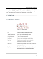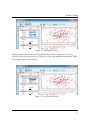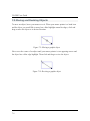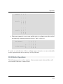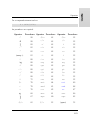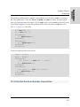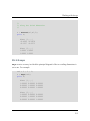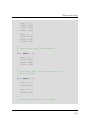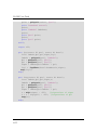
Download AEG FN 6.19 E User guide

 ™
GAUSS
User Guide
Information in this document is subject to change without notice and does not represent a commitment on the part of Aptech Systems, Inc. The software described in thisdocument is furnished under a license agreement or nondisclosure agreement. The software may be used or copied only in accordance with the terms of the agreement.The purchaser may make one copy of the software for backup purposes. No part ofthis manual may be reproduced or transmitted in any form or by any means, electronic or mechanical, including photocopying and recording, for any purpose other than thepurchaser’s personal use without the written permission of Aptech Systems, Inc.
©Copyright Aptech Systems, Inc. Black Diamond, WA 1984-2013
All Rights Reserved Worldwide.
SuperLU. ©Copyright 2003, The Regents of the University of California, through Lawrence Berkeley National Laboratory (subject to receipt of any required approvals from U.S. Dept. of Energy). All Rights Reserved. See GAUSS Software Product License for additional terms and conditions.
TAUCS Version 2.0, November 29, 2001. ©Copyright 2001, 2002, 2003 by Sivan Toledo, Tel-Aviv University, [email protected]. All Rights Reserved. See GAUSS Software License for additional terms and conditions.
Econotron Software, Inc. beta, polygamma, zeta, gammacplx, lngammacplx, erfcplx,
erfccplx, psi, gradcp, hesscp Functions: ©Copyright 2009 by Econotron Software,Inc. All Rights Reserved Worldwide.
GAUSS, GAUSS Engine and GAUSS Light are trademarks of Aptech Systems, Inc.
GEM is a trademark of Digital Research, Inc.
Lotus is a trademark of Lotus Development Corp.
HP LaserJet and HP-GL are trademarks of Hewlett-Packard Corp.
PostScript is a trademark of Adobe Systems Inc.IBM is a trademark of International Business Machines Corporation
Hercules is a trademark of Hercules Computer Technology, Inc.
GraphiC is a trademark of Scientific Endeavors Corporation
i
Tektronix is a trademark of Tektronix, Inc.
Windows is a registered trademark of Microsoft Corporation.
Other trademarks are the property of their respective owners.
The Java API for the GAUSS Engine uses the JNA library. The JNA library is covered under the LGPL license version 3.0 or later at the discretion of the user. A full copy of this license and the JNA source code have been included with the distribution.
Part Number: 008471
Version 13
Documentation Revision: 1781
6/14/2013
ii
Contents
Contents
1 Introduction
1-1
1.1 Product Overview
1-1
1.2 Documentation Conventions
1-1
2 Getting Started
2-1
2.1 Installation Under Linux
2-1
2.2 Installation Under Windows
2-2
2.2.1 Machine Requirements
2-2
2.2.2 Installation from Download
2-3
2.2.3 Installation from CD
2-3
3 Introduction to the GAUSS Graphical User Interface
3-1
3.1 Page Organization Concept
3-1
3.2 Command Page
3-3
3.2.1 Menus and Toolbars
3-4
3.2.2 Command Page Toolbar
3-6
3.2.3 Working Directory Toolbar
3-7
3.2.4 Command History Toolbar
3-7
3.2.5 The Action List Toolbar
3-8
3.3 Layout
3.3.1 Command History Window
3-9
3-10
iii
GAUSS User Guide
3.4 Command Line History and Command Line Editing
3.4.1 Error Output Window
3.5 Source Page: Editing Programs
3-12
3-13
3.5.1 Menus and Toolbars
3-13
3.5.2 Layout and Usage
3-14
3.5.3 Find and Replace
3-22
3.5.4 Changing Editor Properties
3-24
3.5.5 Error Output Window
3-26
3.5.6 The Source Browser: Advanced Search and Replace
3-26
3.6 Data Page
3-29
3.6.1 Menu Bar
3-30
3.6.2 Layout
3-32
3.6.3 Symbol Editor
3-35
3.7 Debug Page
3-37
3.7.1 Menus and Toolbars
3-37
3.7.2 Using Breakpoints
3-40
3.7.3 Stepping Through a Program
3-41
3.7.4 Viewing Variables
3-43
3.8 Help Page
4 Navigating the GAUSS Graphical User Interface
4.1 Hot Keys and Shortcuts
iv
3-12
3-45
4-1
4-1
Contents
4.2 Navigating Between Pages
4-2
4.3 Focus Program Output on I/O
4-3
4.4 F1 Help
4-3
4.5 CTRL+F1 Source Browsing
4-4
5 Using the GAUSS Debugger
5-1
5.1 Starting the Debugger
5-1
5.2 Examining Variables
5-3
5.3 The Call Stack Window
5-5
5.4 Ending Your Debug Session
5-6
6 GAUSS Graphics
6-1
6.1 Overview
6-1
6.2 Basic Plotting
6-2
6.2.1 Plotting multiple curves
6.3 Plot Customization
6.3.1 Using the Graphics Preferences Settings Window
6.4 PlotControl Structures
6-3
6-4
6-4
6-7
6.5 Adding Data to Existing Plots
6-11
6.6 Creating Subplots
6-13
6.6.1 Creating Mixed Layouts
6-16
6.6.2 Creating Custom Regions
6-17
6.7 Time Series Plots in GAUSS
6-18
v
GAUSS User Guide
Understanding the dstart parameter
6-20
6.7.1 Quarterly Example
6-21
6.7.2 Controlling Tic Label Locations
6-22
6.7.3 Tic Label Formatting
6-24
6.8 Interacting with Plots in GAUSS
6-27
6.8.1 Interacting with 2-D Plots
6-28
Hide/Restore Curves
6-28
Relocating Graphic Items
6-29
6.8.2 3-D Plots
Zoom
6-31
Panning and Scrolling
6-31
Rotate/Viewpoint Change
6-31
6.8.3 File Export
6-32
6.8.4 Saving Graphs
6-34
7 Graphics Editing
7-1
7.1 Changing Appearance
7-1
7.2 Adding Items
7-3
7.3 Adding Text to a Text Box
7-4
7.4 Which Object Will Be Edited?
7-4
7.5 Moving and Resizing Objects
7-6
8 Using the Command Line Interface
vi
6-31
8-1
Contents
8.1 Viewing Graphics
8-2
8.2 Command Line History and Command Line Editing
8-2
8.2.1 Movement
8-3
8.2.2 Editing
8-4
8.2.3 History Retrieval
8-5
8.3 Interactive Commands
8-6
8.3.1 quit
8-7
8.3.2 ed
8-8
8.3.3 browse
8-9
8.3.4 config
8-10
8.4 Debugging
8-11
8.4.1 General Functions
8-12
8.4.2 Listing Functions
8-13
8.4.3 Execution Functions
8-14
8.4.4 View Commands
8-16
8.4.5 Breakpoint Commands
8-17
8.5 Using the Source Browser in TGAUSS
9 Language Fundamentals
8-18
9-1
9.1 Expressions
9-1
9.2 Statements
9-1
9.2.1 Executable Statements
9-2
vii
GAUSS User Guide
9.2.2 Nonexecutable Statements
9.3 Programs
viii
9-3
9-4
9.3.1 Main Section
9-4
9.3.2 Secondary Sections
9-4
9.4 Compiler Directives
9-5
9.5 Procedures
9-8
9.6 Data Types
9-8
9.6.1 Constants
9-8
9.6.2 Matrices
9-9
9.6.3 Sparse Matrices
9-17
9.6.4 N-dimensional Arrays
9-17
9.6.5 Strings
9-18
9.6.6 String Arrays
9-23
9.6.7 Character Matrices
9-25
9.6.8 Date and Time Formats
9-26
9.6.9 Special Data Types
9-27
9.7 Operator Precedence
9-29
9.8 Flow Control
9-31
9.8.1 Looping
9-31
9.8.2 Conditional Branching
9-34
9.8.3 Unconditional Branching
9-35
Contents
9.9 Functions
9-36
9.10 Rules of Syntax
9-37
9.10.1 Statements
9-38
9.10.2 Case
9-39
9.10.3 Comments
9-40
9.10.4 Extraneous Spaces
9-41
9.10.5 Symbol Names
9-42
9.10.6 Labels
9-43
9.10.7 Assignment Statements
9-44
9.10.8 Function Arguments
9-45
9.10.9 Indexing Matrices
9-46
9.10.10 Arrays of Matrices and Strings
9-48
9.10.11 Arrays of Procedures
9-49
10 Operators
10-1
10.1 Element-by-Element Operators
10-1
10.2 Matrix Operators
10-3
10.2.1 Numeric Operators
10-4
10.2.2 Other Matrix Operators
10-8
10.3 Relational Operators
10-9
10.4 Logical Operators
10-12
10.5 Other Operators
10-14
ix
GAUSS User Guide
10.6 Using Dot Operators with Constants
10-19
10.7 Operator Precedence
10-20
11 Procedures and Keywords
11.1 Defining a Procedure
11-2
11.1.1 Procedure Declaration
11-3
11.1.2 Local Variable Declarations
11-4
11.1.3 Body of Procedure
11-6
11.1.4 Returning from the Procedure
11-7
11.1.5 End of Procedure Definition
11-8
11.2 Calling a Procedure
11-8
11.3 Keywords
11-9
11.3.1 Defining a Keyword
11-10
11.3.2 Calling a Keyword
11-12
11.4 Passing Procedures to Procedures
11-12
11.5 Indexing Procedures
11-14
11.6 Multiple Returns from Procedures
11-14
11.7 Saving Compiled Procedures
11-16
12 Random Number Generation in GAUSS
12-1
12.1 Available Random Number Generators
12-1
12.1.1 Choosing a Random Number Generator
12.2 Thread-safe Random Number Generators
x
11-1
12-3
12-4
Contents
12.3 Parallel Random Number Generation
12-5
12.3.1 Multiple Stream Generators
12-6
12.3.2 Block-skipping
12-7
13 Sparse Matrices
13-1
13.1 Defining Sparse Matrices
13-1
13.2 Creating and Using Sparse Matrices
13-2
13.3 Sparse Support in Matrix Functions and Operators
13-4
13.3.1 Return Types for Dyadic Operators
13-5
14 N-Dimensional Arrays
14-1
14.1 Bracketed Indexing
14-3
14.2 ExE Conformability
14-4
14.3 Glossary of Terms
14-5
15 Working with Arrays
15-1
15.1 Initializing Arrays
15-1
15.1.1 areshape
15-2
15.1.2 aconcat
15-4
15.1.3 aeye
15-5
15.1.4 arrayinit
15-6
15.1.5 arrayalloc
15-6
15.2 Assigning to Arrays
15-7
15.2.1 index operator
15-8
xi
GAUSS User Guide
15.2.2 getarray
15-10
15.2.3 getmatrix
15-11
15.2.4 getmatrix4D
15-11
15.2.5 getscalar3D, getscalar4D
15-12
15.2.6 putarray
15-14
15.2.7 setarray
15-14
15.3 Looping with Arrays
15-15
15.3.1 loopnextindex
15-17
15.4 Miscellaneous Array Functions
15.4.1 atranspose
15-19
15.4.2 amult
15-21
15.4.3 amean, amin, amax
15-22
15.4.4 getdims
15-24
15.4.5 getorders
15-24
15.4.6 arraytomat
15-25
15.4.7 mattoarray
15-25
15.5 Using Arrays with GAUSS functions
15-26
15.6 A Panel Data Model
15-29
15.7 Appendix
15-31
16 Structures
16.1 Basic Structures
xii
15-19
16-1
16-1
Contents
16.1.1 Structure Definition
16-1
16.1.2 Declaring an Instance
16-3
16.1.3 Initializing an Instance
16-3
16.1.4 Arrays of Structures
16-5
16.1.5 Structure Indexing
16-5
16.1.6 Saving an Instance to the Disk
16-8
16.1.7 Loading an Instance from the Disk
16-8
16.1.8 Passing Structures to Procedures
16-9
16.2 Structure Pointers
16-10
16.2.1 Creating and Assigning Structure Pointers
16-10
16.2.2 Structure Pointer References
16-11
16.2.3 Using Structure Pointers in Procedures
16-12
16.3 Special Structures
16-14
16.3.1 The DS Structure
16-14
16.3.2 The PV Structure
16-15
16.3.3 Miscellaneous PV Procedures
16-19
16.3.4 Control Structures
16-21
16.4 sqpSolveMT
16-22
16.4.1 Input Arguments
16-22
16.4.2 Output Argument
16-27
16.4.3 Example
16-29
xiii
GAUSS User Guide
16.4.4 The Command File
16-29
17 Run-Time Library Structures
17-1
17.1 The PV Parameter Structure
17-1
17.2 Fast Pack Functions
17-5
17.3 The DS Data Structure
17-6
18 Multi-Threaded Programming in GAUSS
18.1 The Functions
18-1
18.2 GAUSS Threading Concepts
18-3
18.3 Coding With Threads
18-4
18.4 Coding Restrictions
18-6
19 Libraries
19.1 Autoloader
19-1
19-1
19.1.1 Forward References
19-1
19.1.2 The Autoloader Search Path
19-2
19.2 Global Declaration Files
19.3 Troubleshooting
19.3.1 Using .dec Files
20 The Library Tool
xiv
18-1
19-8
19-12
19-13
20-1
20.1 Creating New Libraries
20-1
20.2 Loading a Library
20-4
20.3 Viewing Procedures
20-5
Contents
20.4 Refreshing a Library
21 Compiler
20-5
21-1
21.1 Compiling Programs
21-1
21.1.1 Compiling a File
21-2
21.2 Saving the Current Workspace
21-2
21.3 Debugging
21-3
22 File I/O
22.1 ASCII Files
22-1
22-3
22.1.1 Matrix Data
22-3
22.1.2 General File I/O
22-6
22.2 Data Sets
22-7
22.2.1 Layout
22-7
22.2.2 Creating Data Sets
22-8
22.2.3 Reading and Writing
22-8
22.2.4 Distinguishing Character and Numeric Data
22.3 GAUSS Data Archives
22-10
22-11
22.3.1 Creating and Writing Variables to GDA's
22-11
22.3.2 Reading Variables from GDA's
22-12
22.3.3 Updating Variables in GDA's
22-13
22.4 Matrix Files
22-14
22.5 File Formats
22-15
xv
GAUSS User Guide
22.5.1 Small Matrix v89 (Obsolete)
22-16
22.5.2 Extended Matrix v89 (Obsolete)
22-17
22.5.3 Small String v89 (Obsolete)
22-18
22.5.4 Extended String v89 (Obsolete)
22-19
22.5.5 Small Data Set v89 (Obsolete)
22-19
22.5.6 Extended Data Set v89 (Obsolete)
22-21
22.5.7 Matrix v92 (Obsolete)
22-22
22.5.8 String v92 (Obsolete)
22-23
22.5.9 Data Set v92 (Obsolete)
22-24
22.5.10 Matrix v96
22-25
22.5.11 Data Set v96
22-27
22.5.12 GAUSS Data Archives
22-29
23 Foreign Language Interface
23.1 Writing FLI Functions
23-1
23.2 Creating Dynamic Libraries
23-2
24 Data Transformations
xvi
23-1
24-1
24.1 Data Loop Statements
24-1
24.2 Using Other Statements
24-2
24.3 Debugging Data Loops
24-3
24.3.1 Translation Phase
24-3
24.3.2 Compilation Phase
24-3
Contents
24.3.3 Execution Phase
24.4 Reserved Variables
25 The GAUSS Profiler
25.1 Using the GAUSSProfiler
24-4
24-4
25-1
25-1
25.1.1 Collection
25-1
25.1.2 Analysis
25-2
26 Time and Date
26-1
26.1 Time and Date Formats
26-2
26.2 Time and Date Functions
26-4
26.2.1 Timed Iterations
27 ATOG
26-7
27-1
27.1 Command Summary
27-1
27.2 Commands
27-3
27.3 Examples
27-13
27.4 Error Messages
27-16
28 Error Messages
28-1
29 Maximizing Performance
29-1
29.1 Library System
29-1
29.2 Loops
29-2
29.3 Memory Usage
29-2
29.3.1 Hard Disk Maintenance
29-4
xvii
GAUSS User Guide
29.3.2 CPU Cache
29-4
30 GAUSS Graphics Colors
30-1
31 Reserved Words
31-1
32 Singularity Tolerance
32-1
32.1 Reading and Setting the Tolerance
32-2
32.2 Determining Singularity
32-2
33 Publication Quality Graphics
33-1
33.1 General Design
33-1
33.2 Using Publication Quality Graphics
33-2
33.2.1 Getting Started
33-3
33.2.2 Graphics Coordinate System
33-7
33.3 Graphic Panels
33.3.1 Tiled Graphic Panels
33-8
33.3.2 Overlapping Graphic Panels
33-9
33.3.3 Nontransparent Graphic Panels
33-10
33.3.4 Transparent Graphic Panels
33-11
33.3.5 Using Graphic Panel Functions
33-12
33.3.6 Inch Units in Graphic Panels
33-14
33.3.7 Saving Graphic Panel Configurations
33-15
33.4 Graphics Text Elements
33.4.1 Selecting Fonts
xviii
33-7
33-15
33-17
Contents
33.4.2 Greek and Mathematical Symbols
33-18
33.5 Colors
33-19
33.6 Global Control Variables
33-19
34 PQG Fonts
34-1
34.1 Simplex
34-1
34.2 Simgrma
34-2
34.3 Microb
34-3
34.4 Complex
34-4
35 PQG Graphics Colors
35-1
xix
1 Introduction
1.1 Product Overview
GAUSSTM is a complete analysis environment suitable for performing quick calculations, complex analysis of millions of data points, or anything in between. Whether you are new to computerized analysis or a seasoned programmer, the GAUSS family of products combine to offer you an easy to learn environment that is powerful and versatile enough for virtually any numerical task. Since its introduction in 1984, GAUSS has been the standard for serious number crunching and complex modeling of large-scale data. Worldwide acceptance and use in government, industry, and the academic community is a firm testament to its power and versatility. The GAUSS System can be described several ways: It is an exceptionally efficient number cruncher, a comprehensive programming language, and an interactive analysis environment. GAUSS may be the only numerical tool you will ever need. 1.2 Documentation Conventions
The following table describes how text formatting is used to identify GAUSS programming elements: Text Style
regular text
Use
Example
narrative
"... text formatting is 1-1
GAUSS User Guide
used ..."
1-2
bold text
emphasis
"...not supported
under UNIX."
italics
variables "... If vnames is a string or has fewer elements than x has columns, it will be ..."
monospace
code example if scalerr(cm);
cm = inv(x);
endif;
monospace
filename, path, etc. "...is located in the examples subdirectory..."
monospace
bold
reference to a GAUSS command or other programming element within a narrative paragraph
"...as explained under plotScatter..."
Bold Text
reference to section of the manual "...see Operator
Precedence, Section 10.7 ..." 2 Getting Started
2.1 Installation Under Linux
1. Make a directory to install GAUSS in. NOTE: If you choose to install GAUSS in a directory which does not have write permissions for normal user accounts such as /opt or /usr/local, then you must choose the Advanced Installation and Multi-User Installation options during installation.
2. cd to that directory. 3. Gunzip the .gz file. 4. Untar the .tar file. 5. Run the executable script ginstall. The script will give you the option of a default or advanced install. The default option will install everything under the current directory. The advanced installation allows you to choose a single-user or multi-user installation and also allows you to place the shared libraries that GAUSS depends on in another location. If you choose a multi-user installation, the binaries and most of the rest of the installation will reside in the current directory. Each time a new 2-1
GAUSS User Guide
user (a user that has never started GAUSS on this machine ) starts GAUSS on this machine, GAUSS will create a local working directory for that user under the user's home directory. This local working directory will contain the files and folders that which may be customized by the user. This allows the admin to install GAUSS in a location without universal write privileges. No files will be placed under the home directory of any user who does not start GAUSS.
6. Put the installation directory in the executable path. 7. Install the license. To receive a license and license installation instructions, email [email protected] and include your serial number and hostid. The hostid information of your machine is usually generated automatically during installation and stored in the main GAUSS directory in a file called myhostid.txt. For last-minute information, see README.term. 2.2 Installation Under Windows
Following are the minimum recommended machine requirements and information on how to install GAUSS under Windows. 2.2.1 Machine Requirements
l Operating System and Memory (RAM) requirements: Aptech strongly recommends Windows 7 for greatest performance and reliability. l Windows XP, 256 MB minimum, 2 GB recommended. l Windows Vista 32-bit, 512 MB minimum, 2 GB recommended. l Windows Vista 64-bit, 1 GB minimum, 2 GB or more recommended. l Windows 7 32-bit, 1 GB minimum, 2 GB or more recommended. l Windows 7 64-bit, 2 GB minimum, 4 GB or more recommended. 2-2
Getting Started
l Windows 8 32-bit, 1 GB minimum, 2 GB or more recommended. l Windows 8 64-bit, 2 GB minimum, 4 GB or more recommended. l Minimum of 200 MB free hard disk space, more may be needed depending on the size of matrices and the complexity of the program. l Minimum of 128 MB of RAM for video is required to run 3-D graphics. A dedicated graphics card is not required.
l Monthly defragmenting is recommended for traditional hard drives. Solid-state drives should not be defragmented. 2.2.2 Installation from Download
For information on downloading and download instructions, email [email protected] .
2.2.3 Installation from CD
Insert the G
AUSS c ompact disc into the CD-ROM drive, and setup should s tart automatically. If setup does not start automatically, browse to the CD-ROM d rive, and double-click on the * .msi f ile to launch the i nstaller.
You can use this procedure for the initial installation of G
AUSS, and for a dditions or modifications to G
AUSS c omponents.
Obtaining a license
To receive a license and license installation instructions, email l [email protected] a nd include your serial number and hostid. The h ostid information of your machine is usually generated automatically during installation and stored in the main G
AUSS d irectory in a file called myhostid.txt.
2-3
3 Introduction to the GAUSS Graphical
User Interface
3.1 Page Organization Concept
The G
AUSS g raphical user interface is organized into separate ''pages.'' Pages are separate, customizable, m
ain windows with their own set of widgets. Each page is designed to facilitate the performance of one of the c ommon tasks performed in G
AUSS: entering commands interactively, editing a program, examining data, viewing graphs, d ebugging a program, and accessing the help system. Each page is a tab on the main application, allowing you t o instantly access a window custom configured for the task you wish to perform. The G
AUSS g raphical user i nterface is composed of six different pages.
3-1
GAUSS User Guide
Figure 3.1: GAUSS page organization
3-2
Command Page
For executing interactive commands.
Source Page
For editing program files.
Data Page
For examining and editing GAUSS matrices and other data.
Debug Page
For interactively debugging your programs.
Graphics Page
For viewing and interacting with graphs.
Help Page
For accessing the GAUSS help system.
Introduction to the GAUSS GUI
Each page may be undocked from the main application and redocked by toggling the Dock button on the right s ide of the status bar. Navigation between an undocked page and the main application may be accomplished with ALT+TAB and A
LT+SHIFT+TAB. To navigate between pages, use CTRL+TAB to cycle forward and C
TRL+SHIFT+TAB to cycle backwards between pages.
Each page has its own toolbars and menus. The menus and toolbars facilitate intuitive navigation through the GUI a s well as performing desired functions. For example, clicking the N
ew t oolbar button from any page in the GUI will b ring the Source Page to the top of the window stack with a new file opened ready for editing. More d etails on navigating the GUI are in NAVIGATING THE GAUSS GRAPHICAL USER INTERFACE, CHAPTER 4 .
3.2 Command Page
The Command Page is for entering interactive commands to G
AUSS . 3-3
GAUSS User Guide
Figure 3.2: Command Page
3.2.1 Menus and Toolbars
Command Page
File Menu
3-4
New
Creates a new, untitled file in a programming editor on the Source Page. Open File
Opens an existing file in a programming editor on the Source Page. Introduction to the GAUSS GUI
Open Graph
Opens a previously created GAUSS graph (.plot file).
Print
Prints selected text. Recent Files
Holds a selectable dropdown list of recently edited files. Exit
Exits a GAUSS session. Edit Menu
Undo
Restores your last unsaved change. Redo
Re-inserts changes removed with undo. Cut
Removes selected text and copies it to the clipboard. Copy
Copies selected text to the clipboard. Paste
Copies the clipboard contents to the cursor position. Tools Menu
Preferences
Allows you to configure the GAUSS user environment. Install Application
Opens an installation wizard to install a GAUSS application package. Change Font
Allows you to specify a new font. Aptech recommends using a monospaced font such as Courier. Clear Action List
Clears the recent files from the action list menus.
Change Working Allows you to browse for a new working directory. 3-5
GAUSS User Guide
Directory
Clear Working Directory History
Deletes the contents of your working directory history. Recent Working Directories
Contains a dropdown list of your most recent working directories. View Menu
The View menu lets you toggle on or off the windows on the current page.
Help Menu
Goto Help
Takes you to the Help Page. About GAUSS
Provides information regarding your version of GAUSS .
3.2.2 Command Page Toolbar
Figure 3.3: Command Page Toolbar
New
3-6
Opens a new, untitled document in a programming editor on the Source Page and brings you to the Source Page. Open
Opens an existing file for editing. Cut
Removes selected text and places it on the clipboard. Introduction to the GAUSS GUI
Copy
Copies selected text to the clipboard. Paste
Copies the clipboard contents to the cursor position. Print
Prints selected text. Run
Runs the file at the top of the Action List. Debug
Debugs the file at the top of the Action List. Edit
Opens the file at the top of the Action List. Stop Program
Stops a running GAUSS program. 3.2.3 Working Directory Toolbar
The Working Directory Toolbar contains a dropdown list that shows your current working directory a nd a history of recent directories. The Change Working Directory button allows you to browse for and s elect a new working directory.
Figure 3.4: Working Directory Toolbar
3.2.4 Command History Toolbar
3-7
GAUSS User Guide
Figure 3.5: Command History Toolbar
Run
Executes the highlighted command from the command history. Paste
Pastes the highlighted command to the Program Input/Output Window for further editing. Search Previous
Searches the Command Output Window for previous executions of a command and its output. Search Next
Searches the Command Output Window for the next execution of a command and its output. 3.2.5 The Action List Toolbar
Immediately to the right of the Run, Debug, and Edit buttons is a downward pointing triangle. Clicking on this triangle reveals the Action List. The Action List is a selectable drop down list of your most recently acted upon files. The Run, Debug, and Edit buttons share the same Action List. You may add a file to the Action List by running it from the command line or while editing a file, click on the drop down menu from Run, Debug, or Edit, and select Current File. Clicking on the Run button will run the file on the top of the Action List. Placing your mouse over the Run Button produces a tooltip indicating which file will be run. To run one of the other files in the list, access the Action List by clicking on the triangle next to the Run button and select the name of the file you wish to run. The Debug and Edit buttons work in the same manner. 3-8
Introduction to the GAUSS GUI
Figure 3.6: Action List Toolbar
3.3 Layout
The Command Page contains three main widgets: the Program Input/Output Window, the Command History Window, and the Error Output Window, which appears when GAUSS encounters an error. Figure 3.7: Command Page Widgets
3-9
GAUSS User Guide
The Program Input/Output Window allows the user to enter interactive commands as well as displaying any output from a program run. It is also the location for user input requested by the GAUSS functions keyw and cons. 3.3.1 Command History Window
The Command History Window contains a list of recently executed commands. Commands in the command history can be executed by double clicking them or highlighting a command and clicking the Run button from the Command History toolbar. Figure 3.8: Command History Window
Commands can be sent to the Program Input/Output Window for further editing before executing by highlighting a command and clicking the Paste button. The Search Next and Search Previous buttons will search the window forward or backwards for previous executions of that command so that you may inspect its output. Context Menu
3-10
Introduction to the GAUSS GUI
Figure 3.9: Command History
Right-click in the Command History Window to bring up the context menu with the following options: Copy
Copies the highlighted entry to the clipboard.
Delete
Deletes the highlighted entry.
Clear Window
Deletes all Command History entries.
Send to File
Creates a new source file containing the highlighted commands. Toggle View Mode
Toggles between session mode and date mode. 3-11
GAUSS User Guide
3.4 Command Line History and Command Line Editing
When you run a command at the G
AUSS p rompt, it is added to your command line history. The last 1,000 commands e xecuted at the G
AUSS c ommand line are stored. T
he following keystrokes are supported for m
ovement and editing at the command line and for retrieving the command line history:
Left Arrow
Moves cursor left one character.
Right Arrow
Moves cursor right one character.
HOME
Moves cursor to beginning of line.
END
Moves cursor to end of line.
CTRL+Left Arrow
Moves cursor left one word.
CTRL+Right Arrow
Moves cursor right one word.
Up Arrow
Search up through command history.
Down Arrow
Search down through command history.
NOTE: Use CTRL+PAGE-UP or CTRL+PAGE-DOWN to scroll through your program output in the program input/output window.
3.4.1 Error Output Window
The Error Output Window shows errors messages from program runs or interactive commands. It may be viewed from any page by clicking the Error Output button on the right side of the status bar. The Error Window will automatically open when an error occurs. It will close and empty its contents on the next program run or interactive command. 3-12
Introduction to the GAUSS GUI
Double-clicking on the first line of the error will bring you to the file and line on which the error occurred. Figure 3.10: Error Window
3.5 Source Page: Editing Programs
The Source Page is for creating and editing programs and procedures. 3.5.1 Menus and Toolbars
Section 3.2 provides details of the main menus and toolbars. The Source Page contains the following additional menu options. File Menu
Save
Saves the active file.
Save As
Saves the active file with a new or different file or path name.
Close
Closes the selected file.
Close All
Closes all open files.
Window Menu
3-13
GAUSS User Guide
Split File Buffer Horizontally
Horizontally splits the active file into two views.
Split File Buffer Vertically
Vertically splits the active file into two views.
Split Tab Stack Horizontally
Tiles any open programming editors horizontally.
Split Tab Stack Vertically
Tiles any open programming editors vertically.
Remove Tab Split
Removes any editor window tiling.
Remove Buffer Split
Removes a buffer split in the active file.
3.5.2 Layout and Usage
The Source Page contains four separate window components, Program Input/Output, Bookmarks, Active Libraries, and Programming Editor.
3-14
Introduction to the GAUSS GUI
Figure 3.11: Source Page
Programming Editor
Individual programming editors are opened in the editor docking area. The editor docking area allows tabbing of multiple open files, with the option to tile editors with a horizontal or vertical split. Select W
indow->Split Horizontally or Window->Split Vertically to tile open editor windows.
3-15
GAUSS User Guide
Figure 3.12: Programming Editor
Programming editor features:
1. Syntax highlighting:The GAUSS programming editor will provide syntax highlighting for G
AUSS, C/C++, Java, Fortran, R and many other languages. 2. Autocompletion:Autocompletion is available in the G
AUSS p rogramming editor for G
AUSS f unctions and for structure members of any structure in an active GAUSS library. 3-16
Introduction to the GAUSS GUI
Figure 3.13: Autocomplete
Using autocomplete: if the characters you enter match items in the autocomplete list, a dropdown box will a ppear containing those functions. To navigate the dropdown list, press the down arrow or continue typing u ntil only one selection remains. Once the desired command is highlighted, press the ENTER key to insert the remainder of the word. The editor will provide autocomplete for the members of any structures that are in a GAUSS library if: the library is loaded, the file contains a statement to load the library, or the structure definition is in the current file.
3. Function Call Tooltips:After a GAUSS command and an opening parenthesis has been entered, a tooltip will appear w
ith the argument list for the function. Figure 3.14: Tooltips
4. Function Browser:Dropdown list lists all procedures defined in your file and lists their arguments. Select a procedure from the list to navigate to its definition. 3-17
GAUSS User Guide
Figure 3.15: Function Browser
5. Code folding:At the start of code blocks (e.g., procedure definitions, do and f
or loops, and if s tatements), the left margin of the programming editor will contain a +. Clicking t he + will hide the block of code from view and place a horizontal line across the editor indicating folded c ode and changing the + to a -. Clicking on the - will reveal the hidden code. Figure 3.16: Code folding of 'if' block
3-18
Introduction to the GAUSS GUI
6. Autoindenting: T
he GAUSS programming editor provides automatic code indenting and deindenting. Autoindenting n ot only simplifies the process of writing code but also encourages the creation of readable code. 7. Variable highlighting:Click on a variable name and all instances of that variable will be highlighted. Figure 3.17: Variable highlighting
8. Find usages: Right click on a variable or procedure and select 'Find Usages' from the context menu to create an organized clickable list of all usages in your file. 3-19
GAUSS User Guide
Figure 3.18: Find usages
9. Bookmarks:Bookmarks allow quick navigation to often visited lines of code. To insert a bookmark, hold down the SHIFT key and left click in the left margin of the file on the line where you would like to set the bookmark. If a file contains more than one bookmark, you may use F2 to navigate to the next bookmark in the file. To navigate between bookmarks in multiple files, use the bookmark window. The bookmark window contains a list of all of your bookmarks.
Double-click on a listed bookmark and G
AUSS w
ill bring you to the file and line of your bookmark regardless of whether the file is already open for editing or not.
10. Source code formatting: T
he GAUSS editor will correctly format a source file with incorrect formatting. This is available f rom the context menu or with the hot 3-20
Introduction to the GAUSS GUI
key CTRL+I.
Programming Editor Hot Keys
CTRL+A
Select All.
CTRL+C
Copy.
CTRL+D
Debug current file.
CTRL+F
Find and replace.
CTRL+G
Go to line.
CTRL+I
Formats the current file.
CTRL+L
Delete line.
CTRL+N
Open new file.
CTRL+O
Open existing file.
CTRL+P
Print file.
CTRL+/
Used for block commenting.
CTRL+R
Run current file.
CTRL+S
Save current file.
CTRL+T
Switches current line with the line above.
CTRL+V
Paste.
CTRL+W
Closes the current file.
3-21
GAUSS User Guide
CTRL+Z
Undo.
CTRL+Y
Redo.
CTRL+~
Cycles through open editor windows.
CTRL+F1
Go to definition of function under cursor.
F1
Go to Help Page for function under cursor.
SHIFT+F1
Open inline help for function under cursor.
3.5.3 Find and Replace
From the Edit Menu, selecting Find and Replace or pressing CTRL+F will bring up the find and replace widget at the bottom of your open programming editor. If a word is highlighted when you access find and replace, it will automatically be present in the find box when the find and replace widget is opened. Press the ENTER key or > to search forward. Press the < button to search backwards. To close the find and replace widget, press ESC or click the button on the left. 3-22
Introduction to the GAUSS GUI
Figure 3.19: Find and Replace
The Replace Box has three buttons: > means replace the highlighted expression and search forwards, < means replace the highlighted expression and search backwards and replace means replace the highlighted text and do not change the cursor position. Regular Expressions
Find and Replace in GAUSS supports regular expression searching. Regular expression searching gives users tremendous power allowing quick and precise search and replace throughout an entire file. For example, let us start with a file containing the following commands: r
c
x
y
z
=
=
=
=
=
100;
50;
rndn(r,c);
rndu(r,c);
x.*rndn(r,c);
3-23
GAUSS User Guide
Regular expressions allow you to perform very specific find and replace commands. Suppose that we want to find all usages of rndu and rndn and replace them with rndKMu. Figure 3.20: Find and Replace Regular Expression
To open Find and Replace, we enter CTRL+F in out open text editor. In the Find and Replace widget, select the check box next to Regex to enable regular expression searching. One of the most simple regular expression options is to a dd a '.'. The '.' means any character. So, if we search for "rnd." that will find any string that contains rnd followed by any character, such as rnda, rndb, rndc, rndn, rndu, etc. Now enter "rndKMu" in the replace box and click Replace All. Now all instances of rndu and rndn should be replaced with rndKMu. 3.5.4 Changing Editor Properties
Programming editor preferences can be accessed by selecting: Tools->Preferences from the menu bar. From the Preferences window, select Source from the tree on the 3-24
Introduction to the GAUSS GUI
left. Here you can customize the programming editor's behavior. Figure 3.21: Editor Preferences
The editor preferences has three main sections:
General Settings
The general settings are located on the top left. Colors
This section is located along the bottom half of the preferences dialog window. Click one of the color buttons to change an element in the color scheme used in the editor.
Autocomplete Settings
On the top right of the Source Preferences, under the heading "Autocompletion Source" , are the controls for autocompletion settings. This allows you to choose the contents of your dropdown autocomplete suggestions. The options are:
3-25
GAUSS User Guide
GAUSS Library Provides autocomplete suggestions for GAUSS intrinsic functions.
Current Document Provides autocomplete suggestions for all variables, procedures, GAUSS functions and keywords that are used in the file.
Both
Provides autocomplete suggestions for both above.
None Turns off autocomplete suggestions in the editor.
3.5.5 Error Output Window
The Error Output Window can be accessed by toggling the Error Output button on the right side of the status bar. For details regarding the features and usage of the Error Output Window, see Section 3.4.1 . Figure 3.22: Error Output Window
3.5.6 The Source Browser: Advanced Search and Replace
The Source Browser is a powerful search and replace tool that makes it much easier to work with your code--especially larger projects. You may open the source browser by selecting View->Source Browser from the Source Page, or entering the hot-key SHIFT+CTRL+F.
3-26
Introduction to the GAUSS GUI
Figure 3.23: Source Browser
The source browser is made up of two main sections. On the left are the control tabs and on the right is the results display. The first of the control tabs is the Search tab. In this tab you enter your search query. You can specify a specific file pattern or filename to search and also the directory within which to search. The button with three dots [...] to the right of the directory dropdown menu is a browse button that will open a dialog window that will allow you to browse to locate the desired directory.
Figure 3.24: Search and Replace
3-27
GAUSS User Guide
The Advanced tab allows you to refine your search criteria. Checking the References check box will limit your search to only locations where a variable is referenced. Alternatively, checking the Assignments box would limit your search to only those places where the variable was assigned to. For example, if you were searching for the variable 'nobs', this is an assignment:
nobs = 300;
whereas this is a reference:
myVar = nobs - 1;
Figure 3.25: Advanced Search and Replace
You may also select to limit your search to whole words, match case or use regular expressions. This tab also allows you to control whether your search extends to subdirectories and if you would like to exclude files larger than a certain size. It is recommended that you always select Ignore Binaries.
Executing a search
Once you have a search string in the Find box and have your desired parameters set, press the 'search' button to execute your search. In the results display window, you will see a list of files that contain matches to your search. To the left of each file in the list you will see a check box which can be used to include or exclude the matches in a file from any Replace actions. To the right of the file name you will see a number in parentheses which indicates how many matches were found in the file.
3-28
Introduction to the GAUSS GUI
Figure 3.26: Executing a search
Expand the node of a file to examine its list of matches, or right-click and select 'Expand All' from the context menu. Once you expand the node for a file, you will see the line number of the match followed by a colon and then the line of code with the match highlighted in yellow. Double-click on a line to edit that file.
Executing a replace
After you have completed your search and unchecked any matches that you do not want replaced, click the Replace tab. Enter your replacement term and press the Replace button. GAUSS will warn you that any changes in unsaved files cannot be undone. If you are certain of your replacement, click OK.
If you are making a change across a large number of files, particularly if you are not using a version control system like Subversion or Git, it is a good idea to select the 'Backup Original' check box. With this selected, before GAUSS makes the replacements to your file it will save a copy of the original with a .bak extension. For example if your original file was myfile.gss, the backup file will be called myfile.gss.bak.
If you select the 'Overwrite Backup' checkbox, the next time that you make a change to this file, the file myfile.gss.bak will be overwritten. If you do NOT check the 'Overwrite Backup' check box, GAUSS will make incremented backup files: myfile.gss.bak(1), myfile.gss.bak(2), etc.
3.6 Data Page
Section 3.2.1 provides details of the main menus and toolbars. The Data Page contains the following changes to the toolbar and menu options. 3-29
GAUSS User Guide
Figure 3.27: Data Page
l Menu Bar
l Layout
l Symbol Editor
3.6.1 Menu Bar
Symbol Editor Menu
3-30
Edit Symbol
Opens an active symbol from your current GAUSS workspace in a symbol editor.
Save Symbol
Saves changes to the symbol in the active symbol editor.
Introduction to the GAUSS GUI
Reload Symbol
Reloads a symbol that is out-of-sync with the GAUSS symbol table. Note: This only applies if auto-reload mode is turned off. Toggle Auto-reload
Turns on/off autoreload for the active symbol editor. Preferences
Brings up preference dialog for changing the settings of open symbol editors.
Window Menu
Split Horizontally
Tiles open symbol editors horizontally. Split Vertically
Tiles open symbol editors vertically.
Toolbar
Figure 3.28: Data Page Toolbar
New
Opens an active symbol from your current GAUSS workspace in a symbol editor.
Save
Saves changes to the symbol in the active symbol editor.
Reload
Reloads an out-of-sync symbol editor. Note: This applies only if autoreload is disabled.
3-31
GAUSS User Guide
3.6.2 Layout
The Data Page has two main widgets: the symbol tree and the source editor docking area. The Program Input/Output and Error Windows are also accessible from the toggle buttons on the right side of the status bar. The Symbol Tree window lists all of your active symbols, organized by type. To view your active symbols, c lick on the node expander or right click and select Symbol View from the context menu. Hovering over a symbol in the Symbol Tree will produce a tooltip with a preview of the symbol's contents. To view the entire contents of a symbol, double-click the symbol or right-click the symbol and select Edit. The symbol will now appear in a symbol editor (see Symbol Editor, Section 3.6.3 ). 3-32
Introduction to the GAUSS GUI
Figure 3.29: Symbol View
Double-clicking an already open symbol will bring that symbol to the top of the stack of open symbol editors. If you would like to open a second copy of a symbol, right-click on the symbol in the symbol tree and select Edit Another Copy. GAUSS allows you to open more than one copy of each symbol so that you can examine different portions of a large matrix at the same time. Special Case: Structures
3-33
GAUSS User Guide
To view a structure in the GAUSS Symbol Editor, expand the Structures node on the Symbol Tree. From here you will see a full list of all structures in your current GAUSS workspace. Expanding the node of a structure will reveal its members. To view the contents of any member of a GAUSS structure, first open the structure in a Struct Viewer, by either double-clicking or right-clicking and selecting Edit over the name of the structure in the Symbol Tree. Once open in the Struct Viewer, individual members of the structure can be accessed for viewing and editing from the Struct Tree. The Struct Editor
When opened from the Symbol Tree, structures will be loaded into a special Struct Editor. The Struct Editor is composed of a Struct Tree Widget and a Struct Member Editor. The Struct Tree Widget displays the structure being edited and its members names, data types and dimensions. The Struct Member editor displays the contents of individual struct members. The Struct Editor is displayed in the Source Editor docking area like all other Source Editors. 3-34
Introduction to the GAUSS GUI
Figure 3.30: The Struct Editor
Individual structure members can be opened for editing or viewing from the Struct Tree Widget in the same manner as other data types, such as matrices, are opened from the Symbol Tree. Structure members will be opened in a Symbol Editor to the right of the Struct Tree Widget. Multi-dimensional Arrays
Expand the Arrays node and double-click on an array to open it in a symbol editor. Use CTRL+Up-Arrow and CTRL+Down-Arrow to cycle through views of the different dimensions.
3.6.3 Symbol Editor
Symbol editors are like spreadsheets that allow viewing and editing data in your workspace. Data may be viewed in decimal, scientific, hexadecimal, or character representation. Double-clicking in a cell allows you to change its contents. Navigation throughout the cells c an be accomplished with the arrow keys, tab, and the mouse. 3-35
GAUSS User Guide
Figure 3.31: Changing a value inside a symbol editor
To highlight multiple cells, click on the corresponding row or column header. To highlight the entire contents of a symbol editory, c lick in the empty header box that connects the first row header to the first column header. Autoreload
By default, open symbol editors will automatically update when the symbol has been changed programmatically. This behavior is referred to as autoreload. A symbol editor in autoreload mode will show (auto) on its header. The header will also display (sync), indicating that the symbol editor's contents are synchronized with the current value of the symbol in the GAUSS symbol table. If you would like the contents of a particular symbol editor to stay the same even if the value of the symbol is changed by running a program or an interactive command, you 3-36
Introduction to the GAUSS GUI
may disable autoreload for that symbol. If the value of a symbol with autoreload disabled is c hanged in the GAUSS symbol table, the symbol editor will display the message outof-sync. This indicates that the values in the symbol editor are not current. 3.7 Debug Page
3.7.1 Menus and Toolbars
Figure 3.32: Debug Toolbar
Go
Runs the program to the next breakpoint.
Toggle Breakpoint
Sets/Clears a breakpoint at the cursor.
Clear Breakpoints
Clears all breakpoints in a file.
Set Watch
Opens a watch variable in a symbol editor.
Step Into
Runs the next executable line of code in the application and steps into procedures.
Step Over
Runs the next executable line of code, but does not step into procedures.
Step Out
Runs the remainder of the current procedure and stops at the next line in the calling procedure.
3-37
GAUSS User Guide
Run to Cursor
Runs the program until it reaches the cursor position.
Stop
Terminates a debugging session.
Components and Usage
The Debug Page is composed of five main widgets: Breakpoint List
An interactive list of all breakpoints. Call Stack Window
An interactive display of the chain of procedure calls.
Local Variable Window
An interactive display of all variables that are in scope. Variable Dump Window
Displays the full contents of a variable. Watch Window
An interactive display of user specified variables. The Debug Window indicates which line it is on by the >>> located in the left margin. This is also the location where breakpoints are added. To add a breakpoint, click in the left margin of the Debug Window on the line you wish to add the breakpoint. Clicking an active breakpoint will remove it. 3-38
Introduction to the GAUSS GUI
Figure 3.33: Debug Window
Starting and Stopping the Debugger
You can start debugging of a file you are in by pressing CTRL+D. Click the Debug button to debug the file in the top of the Action List. Placing your mouse over the Debug button will reveal a tooltip with the name of this file, or click the downward pointing triangle next to the debug button and select a file from the list. 3-39
GAUSS User Guide
Figure 3.34: Debug Button
When the debugger is started, it will highlight the first line of code to be run. Any breakpoints are shown in the left margin of the window. You can stop debugging at any time by clicking the Stop button on the debug toolbar. 3.7.2 Using Breakpoints
Breakpoints stop code execution where you have inserted them. Breakpoints are normally set prior to running the debugger, but can also be set or cleared during debugging by clicking the Set/Clear Breakpoint option on the Debug menu. Setting and Clearing Breakpoints
To set breakpoints in any part of the file not currently being executed, just click in the left margin of the line on which you would like the breakpoint. Alternatively, you can highlight a line then click Toggle Breakpoint. 3-40
Introduction to the GAUSS GUI
Figure 3.35: Setting Breakpoints
To clear a breakpoint in the file, click on the breakpoint you would like to remove or click a line of code that has a breakpoint set and then click Set/Clear Breakpoint. You can clear all breakpoints from the active file by clicking Clear All Breakpoints. 3.7.3 Stepping Through a Program
GAUSS's debugger includes the ability to step into, step out of, and step over code during debugging. Use Step Into to execute the line of code currently highlighted by the debugger. Figure 3.36: Step In (F8)
3-41
GAUSS User Guide
Use Step Out to execute to the end of the current function without pause and return to the calling function. Figure 3.37: Step Out (F10)
Use Step Over to execute the line of code currently highlighted by the debugger without entering the functions that are called. Figure 3.38: Step Over (F9)
Use Stop to stop the debugger.
3-42
Introduction to the GAUSS GUI
Figure 3.39: Stop
3.7.4 Viewing Variables
GAUSS allows you several ways to view the values of variables during debugging. Hover Tool-tip View
Once the debugger is started, hovering your mouse over a variable name will open tooltip with a preview of the values in the variable. These tooltip views are only intended to give a quick view of the data, so they may not show all data held by the variable. If you need to view more data, click on the variable name and type CTRL+E or click the Set Watch Variable and enter the variable name. You may single-click on a variable in the local variable window, or double-click it to view the variable in a floating symbol editor. Entering CTRL+E will open the variable under your cursor in a floating symbol editor window. Editing Variable Values During Debugging
The debugger integrates the Matrix Editor to edit values of loaded variables, or to use as a watch window to view the changing values of variables as you step through a program.
To view a variable in a symbol editor, highlight the variable in the edit window, or the Program Input/Output Window and then open the Matrix Editor. You can use the menu or toolbar to start the Matrix Editor. Making a Watch Window
3-43
GAUSS User Guide
You can make the Matrix Editor a Watch Window, allowing you to watch the changing value of a variable as the lines of the program are executed. You can activate the Watch Window by clicking Set Watch on the Debug toolbar or by highlighting a variable name in the Debugger Window and pressing CTRL+E. Figure 3.40: Watch Window
You use a Watch Window to see how variables change in value during debugging. Watch variables can be specified prior to running the debugger or during a debugging session. The debugger searches for a watch variable using the following order: 1. A local variable within a currently active procedure. 2. A global variable. 3-44
Introduction to the GAUSS GUI
A watch variable can be the name of a matrix, a scalar, a string array, or a string. For a matrix or a string array, the first element is displayed. If a matrix element is clicked, the Matrix Editor is loaded with the matrix. The matrix elements can be changed during the debugging session. 3.8 Help Page
The Help Page gives you access to the entire GAUSS help system in HTML format. The table of contents tree is on the left. Click the + symbol to expand a particular section of the contents and double-click on the title to view the page. As on the other pages, the Program Input/Output Window and the Error Window are available via toggle buttons on the status bar. It can be helpful to enter an interactive command and/or view error output while simultaneously viewing the relevant documentation. Figure 3.41: Help Page
3-45
GAUSS User Guide
Hot Keys
3-46
F1
Opens the Command Reference section for the highlighted command.
CTRL+F1
Opens a programming editor with the function definition of a highlighted procedure.
SHIFT+F1
Opens a floating Help Window for the highlighted command.
4 Navigating the GAUSS Graphical
User Interface
Navigation of the GAUSS Graphical User Interface is designed to naturally follow your actions. For example, if the action you would like to perform is debugging the file that you are editing, you can either enter CTRL+D to debug or select the file from the Debug Toolbar Button's drop down Action List. Both of these options will begin your debugging session and take you to the Debug Page. Regardless of the method you choose to initiate the action, debugging in this case, the navigation is done for you. The same automatic and intuitive navigation is enabled for many common GAUSS actions, such as opening a new or existing file for editing or using the F1 help. 4.1 Hot Keys and Shortcuts
F2
Navigates to the next bookmark in the Active File.
F3
Find again.
F4
Runs highlighted text.
F5
Run file at top of Action List.
4-1
GAUSS User Guide
F6
Debug file at top of Action List. Inside a debug session, F6 will cause the debugger to run to the next breakpoint, or the end of the file if no breakpoint is set.
F7
Edit file at top of Action List.
F8
Step in (During a debug session).
F9
Step over (During a debug session).
F10
Step out (During a debug session).
The Control Keys operate on a file that is being edited or is open in a Programming Editor and has focus. This file is referred to as the Active File. CTRL+D
Debug the Active File.
CTRL+R
Run the Active File.
4.2 Navigating Between Pages
4-2
CTRL+1
Brings up the Command Page.
CTRL+2
Brings up the Source Page.
CTRL+3
Brings up the Data Page.
CTRL+4
Brings up the Debug Page.
CTRL+5
Brings up the Help Page.
CTRL+TAB
Brings up the next page. For example, CTRL+TAB Navigating the
GAUSS GUI
from the Command Page will bring up the Source Page. CTRL+TAB from the Help Page will wrap and bring up the Command Page.
ALT+TAB
Cycles between any pages that are undocked as well as other open programs.
WINDOW+TAB
Windows only: Cycles between any pages that are undocked as well as other open programs.
Mouse Scroll
Wheel
When floating over any set of tabs, the mouse scroll wheel will cycle through the open tabs. This will work for programming editor tabs, symbol editor tabs, and the main page tabs on the left of the main application.
4.3 Focus Program Output on I/O
Under the Tools->Preferences->Command is a check box entitled Focus Program
Output on I/O. Selecting this option will open up a Program Output Window if any program output is printed or if a ny input is requested by the GAUSS commands key, keyw, or cons. 4.4 F1 Help
If your cursor is on the name of a GAUSS command in an editor, you can press F1 and it will take you to the Command Reference listing for that command. Inside the Help system, highlight command names by double-clicking them to enable F1 help navigation. Shift+F1 Inline Help
Entering SHIFT+F1 when your cursor is on a GAUSS function will open an inline help window that floats above your editor window. 4-3
GAUSS User Guide
Figure 4.1: Inline help window opened with SHIFT+F1
4.5 CTRL+F1 Source Browsing
For procedures that reside in a GAUSS Library (.lcg file), you can browse to the procedure definition and to the initiation of any global variables with CTRL+F1. Like F1 help, set your cursor on the procedure or global variable name and enter CTRL+F1. If it resides in an a ctive library, the source file will be immediately opened in a Programming Editor. To learn more about creating a User Library for your procedures, see LIBRARIES , CHAPTER 19 . 4-4
5 Using the GAUSS Debugger
The GAUSS debugger is a powerful tool to speed up and simplify your program development. Debugging takes place on the Debug Page, which is a full-featured dashboard providing you a wealth of information about the status of your variables and your program every step of the way. 5.1 Starting the Debugger
Figure 5.1: Debug Button
You may start a debug session by selecting the Action List Debug button, by entering CTRL+D from the file that you would like to debug, or by entering debug filename from the command line. GAUSS will bring the Debug Page to the front, and the debug session will begin with the first line of code highlighted, waiting to be run. 5-1
GAUSS User Guide
Figure 5.2: Debug Window
From here you can step through your program line-by-line, or run to a line of interest. To tell the debugger to run to a particular line, you must first set a breakpoint. Setting a breakpoint on a line in your program tells the debugger to pause when it gets to that line. You may set a breakpoint in any source file by simply clicking in the margin to the left of the line numbers. You will see a red dot appear in the margin, and a new entry will be added to the breakpoint window, which can be viewed on both the Source and Debug Pages. New breakpoints can be added before or during a debug session. The Debug Page toolbar gives you the controls you need to navigate during debugging. Hover over any of the buttons to get a tooltip with a description of the button's function and its corresponding hot key. 5-2
Using the GAUSS Debugger
Figure 5.3: Debug Toolbar
Debug Run
Runs to the next breakpoint.
Debug Stop
Stops the debug session.
Toggle Breakpoint
Toggles a breakpoint on the current line.
Clear Breakpoints
Removes all breakpoints from all files.
Examine Variable
Opens a user-specified variable in a floating Symbol Editor window.
Step in
Steps to the next line. If the next line is a procedure, it will step inside this procedure.
Step over
Steps to the next line without stepping into other procedures.
Step out
Runs through the end of the current procedure and stops in the calling file.
Run to cursor
Runs to the location of your cursor as if it were a breakpoint.
5.2 Examining Variables
When the debugger is paused at a line in your program, you may view any of the variables in your GAUSS workspace. GAUSS offers several options for this. The first is through the Local Variable window. This window contains an alphabetical list of every variable that is currently in scope. It also lists the type of the variable (matrix, string, structure, etc.) and its first value. The contents of this window are immediately updated each time you step to a new line of your program. 5-3
GAUSS User Guide
Figure 5.4: >Local Variable Window
A single-click to one of these variables will display its full contents in the symbol dump window. The symbol dump window is a GAUSS symbol editor, similar in appearance to a spreadsheet. Double-clicking on a variable in the Local Variable window opens that variable in a floating symbol editor. Located just below the Local Variable window is the Watch window. The Watch window looks and acts much the same as the Local Variable window, but it holds only variables that you specifically add to it. This allows you to place variables of interest in a smaller list that is easier to scan. 5-4
Using the GAUSS Debugger
Figure 5.5: Symbol Dump Window
You may see a tooltip preview of any variable in your file by floating your cursor over the variable name. Placing your cursor on a variable and pressing CTRL-E will open that variable in a floating symbol editor. 5.3 The Call Stack Window
The Call Stack window is like a map into your program. The top entry in the Call Stack window is always your current location. It lists the name of the procedure you are in, the arguments that this procedure takes, the name of the file it is in, and the line number you are on. The next item in the list displays the same information for the location from which your current procedure was called. The item after that displays the location from which that procedure was called and so on. 5-5
GAUSS User Guide
Figure 5.6: Call Stack Window
This list is interactive. Single-clicking on any of the items in the Call Stack window will bring you to that particular line and file. For example, if you would like to examine the line from which your current procedure was called, click on the second item in the call stack list. Not only will this open that line and file in your Debug window, but it will also update the Local Variable window to display all the variables that exist at that location, as well as their current values. To return to your current location, click the top line in the Call Stack window. 5.4 Ending Your Debug Session
If you would like to terminate a debug session before the debugger has run through the entire program, click the Debug Stop button, located at the top left of the Debug Page. Figure 5.7: Debug stop button
5-6
6 GAUSS Graphics
6.1 Overview
The plotting functionality available in GAUSS is designed to provide intuitive methods for visualizing data using a variety of plot types. The main plot drawing functions are: plotBar
Creates a bar plot. plotBox
Creates a box plot using the box graph percentile method. plotContour
Creates a contour plot. plotHist
Calculates and creates a frequency histogram plot. plotHistF
Creates a histogram plot from a vector of frequencies.
plotHistP
Calculates and creates a percentage frequency histogram plot.
plotLogLog
Creates a 2-dimensional line plot with logarithmic scaling of the both the x and y axes.
plotLogX
Creates a 2-dimensional line plot with logarithmic scaling of the x axis.
plotLogY
Creates a 2-dimensional line plot with logarithmic scaling of the y axis.
plotPolar
Creates a polar plot.
6-1
GAUSS User Guide
plotScatter
Creates a 2-dimensional scatter plot.
plotSurface
Creates a 3-dimensional surface plot.
plotTS
Creates a graph of time series data.
plotXY
Creates a 2-dimensional line plot.
6.2 Basic Plotting
The simplest way to plot data in GAUSS is to use default values for the plot settings, such as line color, line size, legend text, etc. These settings may be changed by the user from the main menu bar: Tools-> Preferences-> Graphics. To create a plot using default plot settings, simply call one of the plotting functions with your data as inputs: //Create a sequential column vector from -5 to 5 with
//101 steps
x = seqa(-5, 0.1, 101);
//Set y to the normal probability density function
y = pdfn(x);
//Plot the data
plotXY(x, y);
6-2
GAUSS Graphics
Figure 6.1: One Curve Plot
6.2.1 Plotting multiple curves
Each column of the input matrices is treated as a separate curve or line on the graph. Below is an example that uses the variables created from the example above and adds an additional line: x = seqa(-5, 0.1, 101);
y1 = pdfn(x);
//Set y2 to the Cauchy probability density function
y2 = pdfCauchy(x, 1, 1);
//Plot the data using the ~ operator to horizontally
//concatenate y1 and y2
//Note that y1 and y2 will be plotted against the same
//x values
plotXY(x, y1~y2);
6-3
GAUSS User Guide
Figure 6.2: Two Curve Plot
6.3 Plot Customization
GAUSS offers two ways to customize your graphs. The first is through the graphics preferences dialog window. The second method for plot customization is using a plotControl structure. 6.3.1 Using the Graphics Preferences Settings Window
Main Graph Settings
The default settings for graphics can be opened from the main application menu bar Tools-> Preferences. Then select Graphics from the list on the top left of the preferences window. The Graphics Preferences are broken up into two categories. The first is the Graph Settings tab which controls the settings that apply to the entire graph, such as background color. 6-4
GAUSS Graphics
Figure 6.3: The Graph Settings Tab
2-D Curve Settings
The second section is the Group tabs. These specify the settings for each curve, set of bars, or set of points. Here you may specify line color, thickness, symbol type, bar fill type and the corresponding legend description. Note that you may specify separate preferences for each plot type: xy, scatter, polar, etc.
6-5
GAUSS User Guide
Figure 6.4: The Group Tab
Click the 'Apply' and 'OK' buttons after making your desired changes. GAUSS will use these preferences for all future graphs that are made without passing in a plotControl structure. As we will see in the next section, these settings will also be the starting point when you create a plotControl structure. These settings may be changed at any time.
Contour/Surface Plot Z-Level Color Settings
Surface/Contour Level Color Settings
If you select the 'Surface' radio button, you will see a 'Colors' tab instead of 'Groups' as shown above. This tab allows you to add and subtract default z-level colors and to also change their order.
Available Actions
Edit a color
Select a color
Delete a color
Change color order
6-6
Double-click the color
Single-click the color
Select a color and click the delete button
Click-and-drag color to desired position, or select a color and click the up or down button GAUSS Graphics
6.4 PlotControl Structures
The GAUSSplotControl structure provides a powerful and flexible method for programmatic control of your graphs in GAUSS. This structure is a c onvenient package that stores all of the information about how you would like a specific graph to be displayed. These structures may be saved to disk and reloaded during a future session or passed on to colleagues. Using a plotControl structure requires just two easy steps: 1. Declare the structure. 2. Initialize the structure. Once these steps are completed, you may change any of the plot settings in the structure. Once the plotControl structure is set how you would like, you can pass it in as the first argument to any of the GAUSS plot-creating functions. Below is an example that draws a graph using a plotControl structure set to default values: //Declare the structure
struct plotControl myPlot;
//Initialize the structure
myplot = plotGetDefaults("xy");
//Create a column vector from -3 to 3 with a step size of 0.1
x = seqa(-3, 0.1, 60);
y = sin(x);
//Plot the data using the plotControl structure
plotXY(myPlot, x, y);
6-7
GAUSS User Guide
Figure 6.5: Plot Using plotControl Structure
The available plotControl setting functions include: 6-8
plotGetDefaults
Applies the user defined default settings for a specified graph type to a plotControl structure.
plotSetBar
Sets the fill style and format of bars in a histogram or bar graph.
plotSetBkdColor
Sets background color of a graph.
plotSetGrid
Controls the settings for the background grid of a plot.
plotSetLegend
Adds a legend to a graph and optionally applies settings.
plotSetLineColor
Sets line colors for a graph.
plotSetLineStyle
Sets line styles for a graph.
plotSetLineSymbol
Sets line symbols displayed on the plotted points of a graph.
plotSetLineThickness
Sets line thickness for a graph.
GAUSS Graphics
plotSetNewWindow
Sets whether new graphs should be drawn in the same window or in a newly created window.
plotSetTitle
Controls the settings for the title for a graph.
plotSetXLabel
Controls the settings for the X-axis label on a graph.
plotSetXTicInterval
Controls the interval between X-axis tic labels and optionally at which X-value to place the first tic label.
plotSetXTicLabel
Controls the formatting and angle of Xaxis tic labels for 2-D graphs.
plotSetYLabel
Controls the settings for the Y-axis label on a graph.
plotSetZLabel
Controls the settings for the Z-axis label on a graph.
Most of these functions begin with plotSet. This has two main advantages. First, you may quickly and easily survey the plotSet options by typing plotSet in a GAUSS editor and scrolling through the auto-complete list without needing to consult the documentation. Second, this convention makes your GAUSS code easy to read and understand. Example
//Declare plotControl structure
struct plotControl myPlot;
//Initialize the structure with the "bar" default values from
//the main application menu Tools->Preferences->Graphics
6-9
GAUSS User Guide
myPlot = plotGetDefaults("bar");
//Create data to plot
x = seqa(1, 1, 10);
y = abs(rndn( 10, 1 ));
//Change plot settings
//Turn off the grid
plotSetGrid(&myPlot, "off");
// Make the background light-gray
plotSetBkdColor(&myPlot, "light gray");
//Set the title, title font and font size
plotSetTitle(&myPlot, "Example Bar Plot", "verdana", 16);
//Draw graph
plotBar(myPlot, x, y);
Figure 6.6: Example Bar Plot
6-10
GAUSS Graphics
Notice in the previous example that the first input to the plotSetTitle function is &myPlot and not just the variable name, myPlot. This is because all of the plotControl setting functions take a structure pointer. The ampersand (&) in front of the variable name makes the input argument a pointer to that structure. Passing structure pointers as arguments is much faster and more efficient than passing an entire structure. The rule for remembering when to use a plotControl structure pointer instead of plotControl structure is simple. If the function you are calling sets a value in the structure, you need to use a structure pointer. In all other cases, use the structure. Fortunately the function completion tooltip in the GAUSS editor will indicate which is required, in case you forget this simple rule. For more information on structures and structure pointers see STRUCTURES , CHAPTER 16 .
6.5 Adding Data to Existing Plots
You may add additional data to 2-D plots. This functionality is accessed through the following: plotAddBar
Adds a set of bars to an existing 2-D graph.
plotAddBox
Adds a box plot to an existing 2-D graph.
plotAddHist
Adds a histogram to an existing 2-D graph.
plotAddHistF
Adds a frequency histogram to an existing 2D graph.
plotAddHistP
Adds a percentage histogram to an existing 2-D graph.
plotAddPolar
Adds a polar plot to an existing polar graph.
plotAddScatter
Adds a scatter plot to an existing 2-D graph.
plotAddXY
Adds an XY line to an existing 2-D graph.
6-11
GAUSS User Guide
Any 2-D plot type may be added to any other 2-D plot type, with the exception of contour plots, polar plots and time series plots. You may add a polar plot to a previous polar plot or a time series plot to a time series plot. Example
//Create and plot multivariate random normal data
rndseed 19823434;
cov = { 1 0.9, 0.9 1 };
mu = { 2, 2 };
y = rndMVn(300, mu, cov);
plotScatter(y[.,1], y[.,2]);
//Create line coordinates and add to scatter plot
x = { -0.3, 4.8 };
y2 = { 0, 4.3 };
plotAddXY(x, y2);
Figure 6.7: Example Adding Data to a Plot
6-12
GAUSS Graphics
The plotAdd functions will not make any styling changes to the existing plot. They may, however, increase the scale of the view if needed to accommodate the new curve. Use the plotAdd functions only to add data to an existing graph. Do not attempt to use them to create a new graph. 6.6 Creating Subplots
GAUSS allows you to create two types of graphs within graphs. The first is called a subplot. In GAUSS a subplot divides the canvas up into tiles of equal size and shape. This functionality is controlled with the plotLayout function. The plotLayout function splits the canvas up into a specified number of rows and columns and also specifies into which cell to draw the next graph. //Divide the canvas into 3 rows and 2 columns
and
//set the next drawn graph to be placed into the
//last position (which is the sixth cell);
//plotLayouts use row major ordering
plotLayout(3, 2, 6);
Figure 6.8: plotLayouts use row major ordering
After calling plotLayout, all future graphs will be placed in the cell location specified by the plotLayout call until plotLayout is called again with new parameters or a call to plotClearLayout is made. A call to plotClearLayout will cause the next graph to be drawn to take up the entire canvas. 6-13
GAUSS User Guide
This next graph, after a call to plotClearLayout, will either draw over any existing
graphs or be drawn in a new window depending on your graphics preferences. This setting can be controlled from the "On graph load" setting, located under Tools-> Preferences-> Graphics. It may also be set with the plotSetNewWindow function. Example
//Divide the canvas into 2 rows and 2 columns
and
//place each successive graph in the next
//available cell
for i( 1, 4, 1);
plotLayout(2, 2, i);
//Plot a percentage histogram with 10*i bins
of
//random normal data
plotHistP(rndn(1e5, 1 ), 10*i);
endfor;
//Clear the layout so future graphs are not
drawn in
//this layout
plotClearLayout();
6-14
GAUSS Graphics
Figure 6.9: Example Subplot
6-15
GAUSS Graphics
GAUSS User Guide
6.6.1 Creating Mixed Layouts
In GAUSS, plotLayouts may not overlap. For this functionality use the plotCustomLayout function. However, you may divide the canvas into sections of different size as long as they do not overlap. Example
//Divide the canvas into a 2x2 grid and fill in the first
//row
plotLayout(2, 2, 1);
plotHistP(rndn(1e5,1), 20);
plotLayout(2, 2, 2);
plotHistP(rndn(1e5, 1), 40);
//Divide the canvas into a 2x1 grid and fill in the bottom
//half, leaving the top section alone
plotLayout(2, 1, 2);
plotHistP(rndu(1e5, 1 ), 80);
Figure 6.10: Example Mixed Layout
6-16
6.6.2 Creating Custom Regions
Custom regions in GAUSS are graphs inside of graphs. They may be placed in any location on the canvas and may be any size. This functionality is controlled by the plotCustomLayout function. It takes the location and size parameters for the custom region as a percentage of the entire canvas. As with plotLayout, these settings will be applied to the next drawn graph. //Draw a custom region that starts 25% of the
//distance from the left edge of the canvas, 10%
//from the bottom of the canvas with a width of 40%
//of the canvas and a height of 28% of the canvas
plotSetCustomRegion(0.25, 0.1, 0.4, 0.28);
Unlike with plotLayout, these custom regions will not delete any graphs below them and can thus be used to place a small graph over a portion of a larger graph. Example
//Draw a full size graph
rndseed 908734;
y = rndn(1e5, 1);
plotHistP(y, 30);
//Draw a custom region, close-up over the bottom left
// of the previously created graph
plotCustomLayout(0.1, 0.3, 0.2, 0.4);
//Set up plotControl struct with simple view
struct plotControl myPlot;
myPlot = plotGetDefaults("box");
plotSetLegend(&myPlot, "off");
plotSetGrid(&myPlot, "off");
plotSetXAxisShow(&myPlot, 0);
plotSetYAxisShow(&myPlot, 0);
6-17
GAUSS Graphics
GAUSS Graphics
GAUSS Graphics
GAUSS User Guide
//Create plot in custom region defined above
plotBox(myPlot, 0, y);
//Clear the layout, so future graphs will not be
//drawn in this custom region
plotClearLayout();
Figure 6.11: Example Custom Layout
6.7 Time Series Plots in GAUSS
GAUSS provides the following functions to simplify the process of creating time series graphics:
plotTS
Creates a graph of time series data. plotSetXTicLabel
Controls the formatting and angle of X-axis tic labels for 2-D time series graphs.
plotSetXTicInterval
Controls the interval between X-axis tic labels and also allows the user to specify the first tic to 6-18
be labeled for 2-D time series graphs.
To create a basic time series plot in GAUSS, you will use the plotTS function. In addition to the y data to plot, this function requires the following inputs:
dstart
Scalar, the starting date of the time series in DT scalar format.
frequency
Scalar, the frequency of the data per year. Valid options include:
12 Monthly
4 Quarterly
1 Yearly data
Example
//Data to plot
y = rndu(24, 1);
//Start the series in January of 1987
dstart = 1987;
//Specify the data as monthly
freq = 12;
//Plot the data
plotTS(dstart, freq, y);
The example program above will create a graph of monthly data from January of 1987 through December of 1988. It should look similar to the graph below:
6-19
GAUSS Graphics
GAUSS Graphics
GAUSS Graphics
GAUSS User Guide
Figure 6.12: Close-up of monthly data plot
Understanding the dstart parameter
The dstart parameter is specified to be a scalar value in DT scalar format. In DT scalar format the leading four digits are the year and the next two digits, if present, represent the month. If the month information is not present, as in the example above, GAUSS will assume the first month of the year. This means that this:
2008
and this:
200801
will both be treated as specifying January of 2008.
To specify a starting quarter in DT scalar format, set the final digits of your dstart to be the first month of the quarter. The following represent 2008 Q1, 2008 Q2, 2008 Q3 and 2008 Q4 respectively.
200801
200804
6-20
200807
200810
6.7.1 Quarterly Example
Using what we have just learned, we will create a quarterly graph that starts at 2007 Q4 and runs for 16 quarters.
//Create 16 random data points
y = rndu(16, 1);
//Start the series in 2007 Q4
dstart = 200710;
//Specify the data as quarterly
freq = 4;
//Plot the data
plotTS(dstart, freq, y);
This should produce a graph that looks similar to this:
6-21
GAUSS Graphics
GAUSS Graphics
GAUSS Graphics
GAUSS User Guide
Figure 6.13: Close-up of quarterly data plot
6.7.2 Controlling Tic Label Locations
The first tic label on the X-axis of the graph that ended the last section is located on the first data point, 2007 Q4. Let us suppose that we would prefer the graph to have tic labels only on the first quarter of each year. We can accomplish this by using the function plotSetXTicInterval.
plotSetXTicInterval has the following parameters:
interval
the number of data points between each X-tic that is labeled.
firstLabeled
the value of the first data point to be labeled.
Since we are working with quarterly data and would like to place X-tic labels on each year, we will set the interval parameter equal to four and we will set the first-
6-22
Labeled to be the first full year in our series, 2008. This will change our program to look like this:
//Declare and initialize plotControl structure
struct plotControl myPlot;
myPlot = plotGetDefaults(“xy”);
//Create 16 random data points
y = rndu(16, 1);
//Start the series in 2007 Q4 and specify
//quarterly data
dstart = 200710;
freq = 4;
//Start x-tic labels at 2008 and label every 4th
//data point
interval = 4;
firstLabeled = 2008;
plotSetXTicInterval(&myPlot, interval, firstLabeled);
//Plot the data
plotTS(myPlot, dstart, freq, y);
This code should create a graph with x-tic labels only on the first quarter of each year as you see below:
6-23
GAUSS Graphics
GAUSS Graphics
GAUSS Graphics
GAUSS User Guide
Figure 6.14: Quarterly data graph
We can see that the X-tics are in the correct location. However since we are only labeling each year, we may not want Q1 printed next to the year on each of the X-tic labels. 6.7.3 Tic Label Formatting
We can change the formatting of these labels and optionally the angle at which they are printed with the function plotSetXTicLabel. This function has the following arguments:
fmt
string, specifying the format with which to format the X-tic labels.
angle
scalar, the angle at which to print the labels
The fmt input can take many forms, see dttostr and strtodt for all options, but for this purpose we are only concerned with these three:
YYYY
6-24
print the four digit year.
QQ
print the quarter as Q1, Q2, Q3 or Q4.
MO
print the month as a two digit number.
These format specifiers can be placed in any order. You may place any characters in between them and they will be printed literally. For example if we start with 201204:
fmt = “YYYY-QQ”;
will tell GAUSS to print the date as:
2012-Q2
whereas:
fmt = “MO/YYYY”;
tells GAUSS to print the date as:
04/2012
Since we want to print only the four digit year on our x-tic labels, we will set:
fmt = “YYYY”;
Giving us the following program:
//Declare and initialize plotControl structure
struct plotControl myPlot;
myPlot = plotGetDefaults(“xy”);
//Create 16 random data points
y = rndu(16, 1);
//Start the series in 2007 Q4 and specify
//quarterly data
6-25
GAUSS Graphics
GAUSS Graphics
GAUSS Graphics
GAUSS User Guide
dstart = 200710;
freq = 4;
//Start x-tic labels at 2008 and label every 4th
//data point
interval = 4;
firstLabeled = 2008;
plotSetXTicInterval(&myPlot, interval, firstLabeled);
//Label X-tics with only the 4 digit year
plotSetXTicLabel(&myPlot, “YYYY”);
//Plot the data
plotTS(myPlot, dstart, freq, y);
This final program should yield a graph that looks similar to:
Figure 6.15: Quarterly data graph
6-26
6.8 Interacting with Plots in GAUSS
Once a graph has been created, GAUSS provides interactive zooming, panning, and the moving of legends and subplots as well as the ability to hide and restore individual curves on the graph. Plot rotation is also available for 3-dimensional plots. 6-27
GAUSS Graphics
GAUSS Graphics
GAUSS Graphics
GAUSS User Guide
6.8.1 Interacting with 2-D Plots
To interact with plots in GAUSS, first select the "Zoom/Pan Plot" button from the toolbar. With this button selected, you will be able to perform actions on the view of a particular plot. Zooming is controlled by the mouse scroll wheel. Scroll the mouse wheel forward to zoom in. Pan and scroll is accomplished by drag-and-drop with the mouse. Note that upon zooming or panning, the axes will be automatically updated to reflect the new view. Figure 6.16: Zoom/Pan Plot Toolbar
Hide/Restore Curves
Each legend item is also a button that hides and restores individual curves, bars, etc. Click on a legend item to hide the corresponding curve. Notice that the axes will automatically scale to the remaining curves. Click the legend item again to restore the curve to the graph. 6-28
Figure 6.17: The legend acts as a button to hide curves
Relocating Graphic Items
To relocate subplots or legends first select the "Revise Layout" button. You may then drag and drop the item to its desired location. Initially, legends will be grouped with their respective graph. This means that when you select and move a graph, its legend will also be selected and maintain its position relative to the graph. You may ungroup a legend from its parent graph by right-clicking the legend and selecting "Ungroup." This legend will no longer move along with its graph. You may regroup the legend to the graph by right-clicking the legend and selecting "Regroup." If you would like to change the z-order of an item in a layout, you may select it, rightclick to bring up the context menu and then choose, either "Send to Front" or "Send to Back." Individual plots and their respective legends will both be affected. 6-29
GAUSS Graphics
GAUSS Graphics
GAUSS Graphics
GAUSS User Guide
Figure 6.18: Drag and drop to relocate the legend
6-30
6.8.2 3-D Plots
Zoom
Zooming in and out on a 3-dimensional graph may be accomplished by use of the mouse scroll wheel. Panning and Scrolling
To move a 3-D image without rotating it, hold down the CTRL key and drag the image to its desired location with your mouse. Rotate/Viewpoint Change
To rotate 3-dimensional plots and examine the graph from different viewpoints, click and drag with the mouse. 6-31
GAUSS Graphics
GAUSS Graphics
GAUSS Graphics
GAUSS User Guide
6.8.3 File Export
GAUSS graphs may be exported to many popular file formats, including BMP, PNG, PS, SVG and PDF. Graphics may be exported programmatically or using the graphical controls. To export a graph programmatically, use the plotSave function, passing in the filename with extension and the dimensions in centimeters for the second argument: //Save the graph just created as mygraph.pdf with a width of
//30 cm and a height of 18 cm
size = { 30, 18 };
plotSave("mygraph.pdf", size);
To export a graph using the graphical controls, select the graph you would like to export and then select File->Export Graph from the main menu. Figure 6.19: Export Options
Once you have selected a filename and clicked the save button, a window with export sizing options will appear. This window has two sections. The first section sets the with and height of your exported image. The second section sets the font sizes. If "Auto size" is checked, GAUSS will automatically scale the fonts so that they will be the same size relative to the size of the graph as they appear when viewed in GAUSS. Otherwise you may specify individual font sizes to use for each text object. For convenience, the font sizes specified for your graph will be automatically entered in the respective field (title, axes and legend). 6-32
Figure 6.20: Export Dialog
6-33
GAUSS Graphics
GAUSS Graphics
GAUSS Graphics
GAUSS User Guide
6.8.4 Saving Graphs
Graphs may be saved and then reloaded later. To save a graph, select the graph you would like to save and then select File-> Save Graph from the main menu. GAUSS graphs are saved in an XML format with a .plot extension. Figure 6.21: Save Graph menu
Graphs may also be saved programmatically with the plotSave function. 6-34
7 Graphics Editing
GAUSS allows you to interactively change most all attributes of a created graph. First create a graph. For demonstration purposes you may run the example program randomwalk.e to create a graph. Next open the Graph Settings window if it is not open already, by selecting View->Graph Settings from the menu bar.
7.1 Changing Appearance
Figure 7.1: Changing Appearance
7-1
GAUSS User Guide
Click on the graph to populate the Graph Settings Window. To change one of the colors, single-click on the color button to bring up a color palette window.
Figure 7.2: Color Palette
To change text for a label or title, double-click the current text and edit the text.
Figure 7.3: Text Options
Double-click font names in the graph settings window to open a font dialog window.
7-2
Graphics Editing
Figure 7.4: Font Options
7.2 Adding Items
The Graphics Page toolbar has buttons for adding
l
l
l
l
Lines and arrows
Rectangles
Ellipses
Text boxes
To add an item, click the appropriate toolbar button and then click and drag to create the object in your graphic window.
7-3
GAUSS User Guide
Figure 7.5: Select the item to add
Figure 7.6: Click and drag to add the object
7.3 Adding Text to a Text Box
To add text to a text box, double-click in the text box. When you see a text cursor (which looks similar to a capital i), you may begin entering text.
7.4 Which Object Will Be Edited?
If a graph or graphics object is actively selected, its border will be highlighted red. Changes made in the Graph Settings window will apply to this selected object. If no object is actively selected, changes made in the Graph Settings window will apply to the last selected object.
7-4
Graphics Editing
Figure 7.7: Highlighted Object
When you place your mouse in the Graph Settings window, if no object is actively selected, the last selected object will be given a blue edge highlight to indicate to which object your changes will be made.
Figure 7.8: Last Selected Object
7-5
GAUSS User Guide
7.5 Moving and Resizing Objects
To move an object, hover your mouse over it. When your mouse pointer is a hand icon and the object you would like to move has a blue highlight around its edges, click and drag to move the object to its desired location.
Figure 7.9: Moving a graphic object
Hover over the corner of an object until your mouse pointer is two opposing arrows and the object has a blue edge highlight. Then click and drag to resize the object.
Figure 7.10: Resizing a graphic object
7-6
8 Using the Command Line Interface
TGAUSS is the command line version of GAUSS. The executable file, tgauss, is located in the GAUSS installation directory. The format for using TGAUSS is: tgauss
flag(s) program program...
-b
Execute file in batch mode and then exit. You can execute multiple files by separating file names with spaces. -l logfile
Set the name of the batch mode log file when using the -b argument. The default is tmp/gauss.log###, where ### is the process ID. -e expression
Execute a GAUSS expression. This command is not logged when GAUSS is in batch mode. -o
Suppress the sign-on banner (output only). -T
Turn the dataloop translator on. -t
Turn the dataloop translator off. 8-1
GAUSS User Guide
8.1 Viewing Graphics
NOTE: Graphics using plot* functions are only available from the graphical user interface. The deprecated Publication Quality Graphics graphics generated .tkf files for graphical output. The default output for these graphics is graphic.tkf. On Windows, you can use vwr.exe to view the graphics file; on UNIX/Linux/Mac, you can use vwrmp. Two functions are available to convert .tkf files to PostScript for printing and viewing with external viewers: the tkf2ps function will convert .tkf files to PostScript (.ps) files, and the tkf2eps function will convert .tkf files to encapsulated PostScript (.eps) files. For example, to convert the file graphic.tkf to a postscript file named graphic.ps use: ret = tkf2ps("filename.tkf", "filename.ps")
If the function is successful it returns 0. 8.2 Command Line History and Command Line Editing
When you run a command at the TGAUSS prompt, it is added to your command line history, which is stored in a file called .gauss_prompt_history in your $(HOME) directory on UNIX/Linux or in your $(HOMEDRIVE)\$(HOMEPATH) directory on Windows. A separate history for commands entered in the command line debugger is stored in a file called .gauss_debug_prompt_history in the same directory. By default, the last 500 commands executed at the TGAUSS and debugger command lines are stored in these files. You can change this number by c hanging prompt_hist_num in your gauss.cfg file. The following keystrokes are supported for movement and editing at the command line and for retrieving the command line history: 8-2
8.2.1 Movement
HOME or CTRL+A
Moves cursor to beginning of line
END or CTRL+E
Moves cursor to end of line
8-3
Using the Command
Line Interface
Using the Command
Line Interface
Using the Command
Line Interface
GAUSS User Guide
8.2.2 Editing
8-4
DELETE or CTRL+D
Deletes character at cursor
BACKSPACE or
CTRL+H
Deletes character left of cursor
CTRL+U
Cuts all characters left of cursor
CTRL+K
Cuts all characters right of cursor, including cursor
CTRL+X
Cuts whole line
ESC (Win only)
Deletes whole line
CTRL+V
Pastes text from buffer to left of cursor
CTRL+T
Transposes character at cursor and character left of cursor
8.2.3 History Retrieval
Up Arrow or
CTRL+P
Retrieves previous line in history
Down Arrow or
CTRL+P
Retrieves next line in history
PAGE UP or CTRL+W
Retrieves previous line in history that matches text to left of cursor
PAGE DOWN or
CTRL+S
Retrieves next line in history that matches text to left of cursor
ALT+H or OPTION+H
Prints prompt history to screen
(MAC only)
!!
Runs last line in history
! num
Runs the num line in history
!- num
Runs the line num before current line in history;
!-1 is equivalent to !!
! text
Runs last line in history beginning with text
ALT+/ or ALT+? or
OPTION+/ (MAC
Prints help screen
only)
Note that some of these keystrokes are mapped differently on different computers. For example, on some computers, SHIFT+RIGHT ARROW behaves the same as RIGHT
ARROW, while ALT+RIGHT ARROW moves the cursor right one word. Therefore, mul-
8-5
Using the Command
Line Interface
Using the Command
Line Interface
Using the Command
Line Interface
GAUSS User Guide
tiple keystroke mappings have been supported to maximize the availability of these commandson any given machine. 8.3 Interactive Commands
This section discusses interactive commands available in TGAUSS.
8-6
8.3.1 quit
The quit command will exit TGAUSS. The format for quit is: quit
You can also use the system command to exit TGAUSS from either the command line or a program (see system in the GAUSS LANGUAGE REFERENCE). The format for system is: system
8-7
Using the Command
Line Interface
Using the Command
Line Interface
Using the Command
Line Interface
GAUSS User Guide
8.3.2 ed
The ed command will open an input file in an external text editor (see ed in the GAUSS LANGUAGE REFERENCE). The format for ed is: ed filename
8-8
8.3.3 browse
The browse command allows you to search for specific symbols in a file and open the file in the default editor. You can use wildcards to extend search capabilities of the browse command. The format for browse is: browse symbol
8-9
Using the Command
Line Interface
Using the Command
Line Interface
Using the Command
Line Interface
GAUSS User Guide
8.3.4 config
The config command gives you access to the configuration menu allowing you to change the way GAUSS runs and compiles files. The format for config is: config
Run Menu
Translator Toggles on/off the translation of a file using dataloop. The translator is not necessary for GAUSS program files not using dataloop. Translator line number tracking Toggles on/off execution time line number tracking of the original file before translation. Line number tracking Toggles on/off the execution time line number tracking. If the translator is on, the line numbers refer to the translated file. Compile Menu
8-10
Autoload Toggles on/off the autoloader. Autodelete Toggles on/off autodelete. GAUSS Library
Toggles on/off the GAUSS library functions. User Library Toggles on/off the user library functions. Declare Warnings Toggles on/off the declare warning messages during compiling. Compiler Trace Includes the following options:
Off Turns off the compiler trace function. File Traces program file openings and closings. Line Traces compilation by line. Symbol Creates a report of procedures and the local and global symbols they reference. 8.4 Debugging
The debug command runs a program under the source level debugger. The format for debug is: debug filename
8-11
Using the Command
Line Interface
Using the Command
Line Interface
Using the Command
Line Interface
GAUSS User Guide
8.4.1 General Functions
8-12
?
Displays a list of available commands.
q/Esc
Exits the debugger and returns to the GAUSS command line.
+/-
Disables the last command repeat function. 8.4.2 Listing Functions
l number
Displays a specified number of lines of source code in the current file. lc
Displays source code in the current file starting with the current line. ll file line
Displays source code in the named file starting with the specified line. ll file
Displays source code in the named file starting with the first line. ll line
Displays source code starting with the specified line. File does not change. ll
Displays the next page of source code. lp
Displays the previous page of source code. 8-13
Using the Command
Line Interface
Using the Command
Line Interface
Using the Command
Line Interface
GAUSS User Guide
8.4.3 Execution Functions
8-14
s number
Executes the specified number of lines, stepping into procedures. n number
Executes the specified number of lines, stepping over procedures. x number
Executes code from the beginning of the program to the specified line count, or until a breakpoint is hit. g
Executes from the current line to the end of the program, stopping at breakpoints. The optional arguments specify other stopping points. The syntax for each optional argument is: filename
line
period
The debugger will stop every period times it reaches the specified line in the named file. filename
line
The debugger will stop when it reaches the specified line in the named file. filename
,, period
The debugger will stop every period times it reaches any line in the named file. line
period
The debugger will stop every period times it reaches the specified line in the current file. filename
The debugger will stop at every line in the named file. line
The debugger will stop when it reaches the specified line in the current file. procedure
period
The debugger will stop every period times it reaches the first line in a called procedure. procedure
The debugger will stop every time it reaches the first line in a called procedure.
j
Executes code to a specified line, procedure, or period in the file without stopping at breakpoints. The optional arguments are the same as g, listed above.
jx number
Executes code to the execution count specified (number) without stopping at breakpoints.
o
Executes the remainder of the current procedure (or to a breakpoint) and stops at the next line in the calling procedure. 8-15
Using the Command
Line Interface
Using the Command
Line Interface
Using the Command
Line Interface
GAUSS User Guide
8.4.4 View Commands
v [[vars]]
Searches for (a local variable, then a global variable) and displays the value of a specified variable. v$[[vars]]
Searches for (a local variable, then a global variable) and displays the specified character matrix. The display properties of matrices and string arrays can be set using the following commands. 8-16
r
Specifies the number of rows to be shown.
c
Specifies the number of columns to be shown.
num, num
Specifies the indices of the upper left corner of the block to be shown.
w
Specifies the width of the columns to be shown.
p
Specifies the precision shown.
f
Specifies the format of the numbers as decimal, scientific, or auto format.
q
Quits the matrix viewer. 8.4.5 Breakpoint Commands
lb
Shows all the breakpoints currently defined. b
Sets a breakpoint in the code. The syntax for each optional argument is: filename
line
period
The debugger will stop every period times it reaches the specified line in the named file. filename
line
The debugger will stop when it reaches the specified line in the named file. filename
,, period
The debugger will stop every period times it reaches any line in the named file. line
period
The debugger will stop every period times it reaches the specified line in the current file. filename
The debugger will stop at every line in the named file. line
The debugger will stop when it reaches the specified line in the current file. procedure
period
The debugger will stop every period times it reaches the first line in a called procedure. 8-17
Using the Command
Line Interface
Using the Command
Line Interface
Using the Command
Line Interface
GAUSS User Guide
procedure
The debugger will stop every time it reaches the first line in a called procedure.
d
Removes a previously specified breakpoint. The optional arguments are the same arguments as b, listed above. 8.5 Using the Source Browser in TGAUSS
To start the Source Browser in TGAUSS, type BROWSE followed by a symbol name. When the Source Browser is active, the prompt displays Browse:. GAUSS searches through all active libraries for the file in which the symbol is defined. If found, the file containing the source code is opened in the default editor. Wildcard (*) searches can also be used. When using wildcard searches, each symbol that the string matches will be displayed on-screen in a numbered list. To select a specific command to view in the default editor, select the number from the list. The Source Browser will remain active until you type CTRL+C to return to the GAUSS prompt. 8-18
9 Language Fundamentals
GAUSS is a compiled language. GAUSS is also an interpreter. A compiled language, because GAUSS scans the entire program once and translates it into a binary code before it starts to execute the program. An interpreter, because the binary code is not the native code of the CPU. When GAUSS executes the binary pseudocode it must "interpret" each instruction for the computer. How can GAUSS be so fast if it is an interpreter? Two reasons. First, GAUSS has a fast interpreter, and the binary compiled code is compact and efficient. Second, and most significantly, GAUSS is a matrix language. It is designed to tackle problems that can be solved in terms of matrix or vector equations. Much of the time lost in interpreting the pseudocode is made up in the matrix or vector operations. This chapter will enable you to understand the distinction between "compile time" and "execution time," two very different stages in the life of a GAUSS program. 9.1 Expressions
An expression is a matrix, string, constant, function reference, procedure reference, or any combination of these joined by operators. An expression returns a result that can be assigned to a variable with the assignment operator '='. 9.2 Statements
A statement is a complete expression or command. Statements end with a semicolon. 9-1
GAUSS User Guide
y = x*3;
If an expression has no assignment operator (=), it will be assumed to be an implicit print statement: print x*3;
or x*3;
Here is an example of a statement that is a command rather than an expression: output on;
Commands cannot be used as a part of an expression. There can be multiple statements on the same line as long as each statement is terminated with a semicolon. 9.2.1 Executable Statements
Executable statements are statements that can be "executed" over and over during the execution phase of a GAUSS program (execution time). As an executable statement is compiled, binary code is added to the program being compiled at the current location of the instruction pointer. This binary code will be executed whenever the interpreter passes through this section of the program. If this code is in a loop, it will be executed each iteration of the loop. Here are some examples of executable statements: y = 34.25;
print y;
9-2
Language
Fundamentals
x = 1 3 7 2 9 4 0 3 ;
9.2.2 Nonexecutable Statements
Nonexecutable statements are statements that have an effect only when the program is compiled (compile time). They generate no executable code at the current location of the instruction pointer. Here are two examples: declare matrix x = 1 2 3 4 ;
external matrix ybar;
Procedure definitions are nonexecutable. They do not generate executable code at the current location of the instruction pointer. Here is an example: zed = rndn(3,3);
proc sqrtinv(x);
local y;
y = sqrt(x);
retp(y+inv(x));
endp;
zsi = sqrtinv(zed);
There are two executable statements in the example above: the first line and the last line. In the binary code that is generated, the last line will follow immediately after the first line. The last line is the call to the procedure. This generates executable code. The procedure definition generates no code at the current location of the instruction pointer. 9-3
GAUSS User Guide
There is code generated in the procedure definition, but it is isolated from the rest of the program. It is executable only within the scope of the procedure and can be reached only by calling the procedure. 9.3 Programs
A program is any set of statements that are run together at one time. There are two sections within a program. 9.3.1 Main Section
The main section of the program is all of the code that is compiled together WITHOUT relying on the autoloader. This means code that is in the main file or is included in the compilation of the main file with an #include statement. ALL e xecutable code should be in the main section. There must always be a main section even if it consists only of a call to the one and only procedure called in the program. 9.3.2 Secondary Sections
Secondary sections of the program are files that are neither run directly nor included in the main section with #include statements. The secondary sections of the program can be left to the autoloader to locate and compile when they are needed. Secondary sections must have only procedure definitions and other nonexecutable statements. #include statements are allowed in secondary sections as long as the file being included does not violate the above criteria. Here is an example of a secondary section: declare matrix tol = 1.0e-15;
proc feq(a,b);
9-4
Language
Fundamentals
retp(abs(a-b) <= tol);
endp;
9.4 Compiler Directives
Compiler directives are commands that tell GAUSS how to process a program during compilation. Directives determine what the final compiled form of a program will be. They can affect part or all of the source code for a program. Directives are not executable statements and have no effect at run-time. They do not take a semicolon at the end of the line. The #include statement mentioned earlier is actually a compiler directive. It tells GAUSS to compile code from a separate file as though it were actually part of the file being compiled. This code is compiled in at the position of the #include statement. Here are the compiler directives available in GAUSS: #define
Define a case-insensitive text-replacement or flag variable. #definecs
Define a case-sensitive text-replacement or flag variable. #undef
Undefine a text-replacement or flag variable. #ifdef
Compile code block if a variable has been #define'd. #ifndef
Compile code block if a variable has not been #define'd. #iflight
Compile code block if running GAUSS Light. #ifunix
Compile code block if running UNIX. #else
Else clause for #if-#else-#endif code block. 9-5
GAUSS User Guide
#endif
End of #if-#else-#endif code block. #include
Include code from another file in program. #lineson
Compile program with line number and file name records. #linesoff
Compile program without line number and file name records. #srcfile
Insert source file name record at this point (currently used when doing data loop translation). #srcline
Insert source file line number record at this point (currently used when doing data loop translation). The #define statement can be used to define abstract constants. For example, you could define the default graphics page size as: #define hpage 9.0
#define vpage 6.855
and then write your program using hpage and vpage. GAUSS will replace them with 9.0 and 6.855 when it compiles the program. This makes a program much more readable.
The #ifdef-#else-#endif directives allow you to conditionally compile sections of a program, depending on whether a particular flag variable has been #define'd. For example: #ifdef log_10
y = log(x);
#else
y = ln(x);
#endif
9-6
Language
Fundamentals
This allows the same program to calculate answers using different base logarithms, depending on whether or not the program has a #define log_10 statement at the top. #undef allows you to undefine text-replacement or flag variables so they no longer affect a program, or so you can #define them again with a different value for a different section of the program. If you use #definecs to define a case-sensitive variable, you must use the right case when #undef'ing it. With #lineson, #linesoff, #srcline, and #srcfile you can include line number and file name records in your compiled code, so that run-time errors will be easier to track down. #srcline and #srcfile are currently used by GAUSS when doing data loop translation. For more information on line number tracking, see Debugging, Section 8.4 and see Debugging Data Loops, Section 24.3 . See also #lineson in the GAUSS LANGUAGE REFERENCE. The syntax for #srcfile and #srcline is different than for the other directives that take arguments. Typically, directives do not take arguments in parentheses; that is, they look like keywords: #define red 4
#srcfile and #srcline, however, do take their a rguments in parentheses (like procedures): #srcline(12)
This allows you to place #srcline statements in the middle of GAUSS commands, so that line numbers are reported precisely as you want them. For example: #srcline(1)
#srcline(2)
#srcline(3)
#srcline(4)
print "Here is a multi-line "
"sentence--if it contains a run-time error, "
"you will know exactly "
"which part of the sentence has the problem.";
The argument supplied to #srcfile does not need quotes: 9-7
GAUSS User Guide
#srcfile(/gauss/test.e)
9.5 Procedures
A procedure allows you to define a new function which you can then use as if it were an intrinsic function. It is called in the same way as an intrinsic function. y = myproc(a,b,c);
Procedures are isolated from the rest of your program and cannot be entered except by calling them. Some or all of the variables inside a procedure can be local variables. local variables exist only when the procedure is actually executing and then disappear. Local variables cannot get mixed up with other variables of the same name in your main program or in other procedures. For details on defining and calling procedures, see PROCEDURES
CHAPTER 11 .
AND
KEYWORDS , 9.6 Data Types
There are four basic data types in GAUSS, matrices, N-dimensional arrays, strings and string arrays. It is not necessary to declare the type of a variable, but it is good programming practice to respect the types of variables whenever possible. The data type and size can change in the course of a program. The declare statement, used for compile-time initialization, enforces type checking. Short strings of up to 8 bytes can be entered into elements of matrices, to form character matrices (For details, see Command Summary, Section 27.1 ). 9.6.1 Constants
The following constant types are supported: Decimal
9-8
Language
Fundamentals
Decimal constants can be either integer or floating point values: 1.34e-10
1.34e123
-1.34e+10
-1.34d-10
1.34d10
1.34d+10
123.456789345
Up to 18 consecutive digits before and after the decimal point(depending on the platform) are significant, but the final result will be rounded to double precision if necessary. The range is the same as for matrices (For details, see Matrices, Section 9.6.2 String
String constants are enclosed in quotation marks: "This is a string."
Hexadecimal Integer
Hexadecimal integer constants are prefixed with 0x: 0x0ab53def2
Hexadecimal Floating Point
Hexadecimal floating point constants are prefixed with 0v. This allows you to input a double precision value exactly as you want using 16 hexadecimal digits. The highest order byte is to the left: 0vfff8000000000000
9.6.2 Matrices
Matrices are 2-dimensional arrays of double precision numbers. All matrices are implicitly complex, although if it consists only of zeros, the imaginary part may take up no 9-9
GAUSS User Guide
space. Matrices are stored in row major order. A 2x3 real matrix will be stored in the following way from the lowest addressed element to the highest addressed element: [1,1] [1,2] [1,3] [2,1] [2,2] [2,3]
A 2x3 complex matrix will be stored in the following way from the lowest addressed element to the highest addressed element:
(real part)
(imaginary part)
[1,1] [1,2] [1,3] [2,1] [2,2] [2,3]
[1,1] [1,2] [1,3] [2,1] [2,2] [2,3]
Conversion between complex and real matrices occurs automatically and is transparent to the user in most cases. Functions are provided to provide explicit control when necessary. All elements of a GAUSS matrix are stored in double precision floating point format, and each takes up 8 bytes of memory. This is the IEEE 754 format:
Bytes
8
Data Type
Significant Digits
floating point
15-16
Range
4.19 x 10-307 <=|X|<=1.67 x 10+308
Matrices with only one element (1x1 matrices) are referred to as scalars, and matrices with only one row or column (1xN or Nx1 matrices) are referred to as vectors. Any matrix or vector can be indexed with two indices. Vectors can be indexed with one index. Scalars can be indexed with one or two indices also, because scalars, vectors, and matrices are the same data type to GAUSS. The majority of functions and operators in GAUSS take matrices as arguments. The following functions and operators are used for defining, saving, and loading matrices: 9-10
[ ]
Indexing matrices. =
Assignment operator.
Language
Fundamentals
|
Vertical concatenation. ~
Horizontal concatenation. con
Numeric input from keyboard. cons
Character input from keyboard. declare
Compile-time matrix or string initialization. let
Matrix definition statement. load
Load matrix (same as loadm). readr
Read from a GAUSS matrix or data set file. save
Save matrices, procedures and strings to disk. saved
Convert a matrix to a GAUSS data set. stof
Convert string to matrix. submat
Extract a submatrix. writer
Write data to a GAUSS data set. Following are some examples of matrix definition statements. An assignment statement followed by data enclosed in braces is an implicit let statement. Only constants are allowed in let statements; operators are illegal. When braces are used in let statements, commas are used to separate rows. The statement let x = 1 2 3, 4 5 6, 7 8 9 ;
or
x = 1 2 3, 4 5 6, 7 8 9 ;
will result in 9-11
GAUSS User Guide
1 2 3
x = 4 5 6
7 8 9
The statement let x[3,3] = 1 2 3 4 5 6 7 8 9;
will result in
1 2 3
x = 4 5 6
7 8 9
The statement let x[3,3] = 1;
will result in
1 1 1
x = 1 1 1
1 1 1
The statement
let x[3,3];
will result in
0 0 0
x = 0 0 0
0 0 0
The statement let x = 1 2 3 4 5 6 7 8 9;
9-12
Language
Fundamentals
will result in
1
2
3
4
x = 5
6
7
8
9
Complex constants can be entered in a let statement. In the following example, the + or - is not a mathematical operator, but connects the two parts of a complex number. There should be no spaces between the + or - and the parts of the number. If a number has both real and imaginary parts, the trailing 'i' is not necessary. If a number has no real part, you can indicate that it is imaginary by appending the 'i'. The statement
let x[2,2] = 1+2i 3-4 5 6i;
will result in
x = 1+2i 3-4i
5
0+6i
Complex constants can also be used with the declare, con and stof statements. An ''empty matrix'' is a matrix that contains no data. Empty matrices are created with the let statement and braces:
x = {};
Empty matrices are supported by several functions, including rows and cols and the concatenation (~, |) operators.
x = {};
hsec0 = hsec;
do until hsec-hsec0 > 6000;
9-13
GAUSS User Guide
x = x ~ data_in(hsec-hsec0);
endo;
You can test whether a matrix is empty by entering rows(x), cols(x) and scalerr
(x). If the matrix is empty rows and cols will return a 0, and scalerr will return 65535.
The ~ is the horizontal concatenation operator and the | is the vertical concatenation operator. The statement y = 1~2|3~4;
will be evaluated as
y = (1~2)|(3~4);
and will result in a 2x2 matrix because horizontal concatenation has precedence over vertical concatenation:
y = 1 2
3 4
The statement
y = 1+1~2*2|3-2~6/2;
will be evaluated as
y = ((1+1) ~ (2*2)) | ((3-2) ~ (6/2));
and will result in a 2x2 matrix because the arithmetic operators have precedence over concatenation: y = 2 4
1 3
For more information, see Operator Precedence, Section 10.7 . 9-14
Language
Fundamentals
The let command is used to initialize matrices with constant values: let x[2,2] = 1 2 3 4;
Unlike the concatenation operators, it cannot be used to define matrices in terms of expressions such as:
y = x1-x2~x2|x3*3~x4;
The statement
y = x[1:3,5:8];
will put the intersection of the first three rows and the fifth through eighth columns of x into the matrix y.
The statement
y = x[1 3 1,5 5 9];
will create a 3x3 matrix y with the intersection of the specified rows and columns pulled from x (in the indicated order).
The following code
let r = 1 3 1;
let c = 5 5 9;
y = x[r,c];
will have the same effect as the previous example, but is more general.
The statement y[2,4] = 3;
9-15
GAUSS User Guide
will set the 2,4 element of the existing matrix y to 3. This statement is illegal if y does not have at least 2 rows and 4 columns. The statement x = con(3,2);
will cause the following prompt to be printed in the window:
- (1,1)
indicating that the user should enter the [1,1] element of the matrix. Entering a number and then pressing ENTER will cause a prompt for the next element of the matrix to appear. Pressing ? will display a help screen, and pressing x will exit.
The statement
load x[] = b:mydata.asc
will load data contained in an ASCII file into an Nx1 vector x. (Use rows(x) to find out how many numbers were loaded, and use reshape(x,N,K) to reshape it to an NxK matrix).
The statement
load x;
will load the matrix x.fmt from disk (using the current load path) into the matrix x in memory.
The statement
open d1 = dat1;
x = readr(d1,100);
will read the first 100 rows of the GAUSS data set dat1.dat. 9-16
Language
Fundamentals
9.6.3 Sparse Matrices
Many GAUSS operators and commands support the sparse matrix data type. You may use any of the following commands to create a sparse matrix: denseToSp
Converts a dense matrix to a sparse matrix. denseToSpRE
Converts a dense matrix to a sparse matrix, using a relative epsilon. packedToSp
Creates a sparse matrix from a packed matrix of nonzero values and row and column indices. spCreate
Creates a sparse matrix from vectors of non-zero values, row indices, and column indices. spEye
Creates a sparse identity matrix. spOnes
Generates a sparse matrix containing only ones and zeros spZeros
Creates a sparse matrix containing no non-zero values. See SPARSE MATRICES , CHAPTER 13 , for more information. 9.6.4 N-dimensional Arrays
Many GAUSS commands support arrays of N dimensions. The following commands may be used to create and manipulate an N-dimensional array: aconcat
Concatenate conformable matrices and arrays in a user-specified dimension. aeye
Create an N-dimensional array in which the planes 9-17
GAUSS User Guide
described by the two trailing dimensions of the array are equal to the identity. areshape
Reshape a scalar, matrix, or array into an array of user-specified size. arrayalloc
Create an N-dimensional array with unspecified contents. arrayinit
Create an N-dimensional array with a specified fill value. mattoarray
Convert a matrix to a type array. See N-DIMENSIONAL ARRAYS , CHAPTER 14 , for a more detailed explanation. 9.6.5 Strings
Strings can be used to store the names of files to be opened, messages to be printed, entire files, or whatever else you might need. Any byte value is legal in a string from 0255. The buffer where a string is stored always contains a terminating byte of ASCII 0. This allows passing strings as arguments to C functions through the Foreign Language Interface. Here is a partial list of the functions for manipulating strings: 9-18
$+
Combine two strings into one long string. ^
Interpret following name as a variable, not a literal. chrs
Convert vector of ASCII codes to character string. dttostr
Convert a matrix containing dates in DT scalar format to a string array. ftocv
Character representation of numbers in NxK Language
Fundamentals
matrix. ftos
Character representation of numbers in 1x1 matrix. ftostrC
Convert a matrix to a string array using a C language format specification. getf
Load ASCII or binary file into string. indcv
Find index of element in character vector. lower
Convert to lowercase. stof
Convert string to floating point. strindx
Find index of a string within a second string. strlen
Length of a string. strsect
Extract substring of string. strsplit
Split an Nx1 string vector into an NxK string array of the individual tokens. strsplitPad
Split a string vector into a string array of the individual tokens. Pads on the right with null strings.
strtodt
Convert a string array of dates to a matrix in DT scalar format. strtof
Convert a string array to a numeric matrix. strtofcplx
Convert a string array to a complex numeric matrix. upper
Convert to uppercase. 9-19
GAUSS User Guide
vals
Convert from string to numeric vector of ASCII codes. Strings can be created like this: x = "example string";
or x = cons;
// keyboard input
or x = getf("myfile",0);
// read a file into a string
They can be printed like this: print x;
A character matrix must have a '$' prefixed to it in a print statement: print $x;
A string can be saved to disk with the save command in a file with a .fst extension and then loaded with the load command: save x;
loads x;
or loads x=x.fst;
The backslash is used as the escape character inside double quotes to enter special characters:
9-20
Language
Fundamentals
"\b"
backspace (ASCII 8)
"\e"
escape (ASCII 27)
"\f"
formfeed (ASCII 12)
"\g"
beep (ASCII 7)
"\l"
line feed (ASCII 10)
"\r"
carriage return (ASCII 13)
"\t"
tab (ASCII 9)
"\\"
a backslash
"\###"
the ASCII character whose decimal value is ''###''.
When entering DOS pathnames in double quotes, two backslashes must be used to insert one backslash: st = "c:\\gauss\\myprog.prg";
An important use of strings and character elements of matrices is with the substitution operator (^). I n the command
create f1 = olsdat with x,4,2;
by default, GAUSS will interpret the olsdat as a literal; that is, the literal name of the GAUSS data file you want to create. It will also interpret the x as the literal prefix string for the variable names: x1 x2 x3 x4. I f you want to get the data set name from a string variable, the substitution operator (^) could be used as: dataset="olsdat";
create f1=^dataset with x,4,2;
9-21
GAUSS User Guide
If you want to get the data set name from a string variable and the variable names from a character vector, use dataset="olsdat";
let vnames=age pay sex;
create f1=^dataset with ^vnames,0,2;
The substitution operator (^) works with load and save also: lpath="/gauss/procs";
name="mydata";
load path=^lpath x=^name;
command="dir *.fmt";
The general syntax is: ^variable_name
Expressions are not allowed. The following commands are supported with the substitution operator (^): create f1=^dataset with ^vnames,0,2;
create f1=^dataset using ^cmdfile;
open f1=^dataset;
output file=^outfile;
load x=^datafile;
load path=^lpath x,y,z,t,w;
loadexe buf=^exefile;
save ^name=x;
save path=^spath;
dos ^cmdstr;
run ^prog;
msym ^mstring;
9-22
Language
Fundamentals
9.6.6 String Arrays
String arrays a re NxK matrices of strings. Here is a partial l ist of the functions for manipulating string arrays:
$|
Vertical string array concatenation operator.
$~
Horizontal string array concatenation operator.
[ ]
Extract subarrays or individual strings from their corresponding array, or assign their values.
'
Transpose operator.
.'
Bookkeeping transpose operator.
declare
Initialize variables at compile time.
delete
Delete specified global symbols.
fgetsa
Read multiple lines of text from a file.
fgetsat
Reads multiple lines of text from a file, discarding newlines.
format
Define output format for matrices, string arrays, and strings.
fputs
Write strings to a file.
fputst
Write strings to a file, appending newlines.
let
Initialize matrices, strings, and string arrays.
loads
Load a string or string array file ( .fst file).
lprint
Print expressions to the printer.
9-23
GAUSS User Guide
lshow
Print global symbol table to the printer.
print
Print expressions on window and/or auxiliary output.
reshape
Reshape a matrix or string array to new dimensions.
save
Save matrix, string array, string, procedure, function or keyword to disk and gives the disk file either a
.fmt , .fst or .fcg extension.
show
Display global symbol table.
sortcc
Quick-sort rows of matrix or string array based on character column.
type
Indicate whether variable passed as argument is matrix, string, or string array.
typecv
Indicate whether variables named in argument are strings, string arrays, matrices, procedures, functions or keywords.
varget
Access the global variable named by a string array.
varput
Assign the global variable named by a string array.
vec
Stack columns of a matrix or string array to form a column vector.
vecr
Stack rows of a matrix or string array to form a column vector.
String arrays a re created through the use of the string array c oncatenation operators. Below is a contrast of the horizontal string and h orizontal string array concatenation operators. The statements:
9-24
Language
Fundamentals
x = "age";
y = "pay";
n = "sex";
s = x$+y$+n;
sa = x$~y$~n;
assign the values: s = agepaysex
s = age
pay
sex
9.6.7 Character Matrices
Matrices can have either numeric or character elements. For convenience, a matrix containing character elements is referred to as a character matrix. A character matrix is not a separate data type, but gives you the ability to store and manipulate data elements that are composed of ASCII characters as well as floating point numbers. For example, you may want to concatenate a column vector containing the names of the variables in an analysis onto a matrix containing the coefficients, standard errors, t-statistic, and p-value. You can then print out the entire matrix with a separate format for each column with one call to the function printfm. The logic of the programs will dictate the type of data a ssigned to a matrix, and the increased flexibility allowed by being able to bundle both types of data together in a single matrix can be very powerful. You could, for instance, create a moment matrix from your data, concatenate a new row onto it containing the names of the variables and save it to disk with the save command. Numeric matrices are double precision, which means that each element is stored in 8 bytes. A character matrix can thus have elements of up to 8 characters. GAUSS does not automatically keep track of whether a matrix contains character or numeric information. The ASCII to GAUSS conversion program ATOG will record the types of variables in a data set when it creates it. The create command will, also. The function vartypef gets a vector of variable type information from a data set. This 9-25
GAUSS User Guide
vector of ones and zeros can be used by printfm when printing your data. Since GAUSS does not know whether a matrix has character or numeric information, it is up to you to specify which type of data it contains when printing the contents of the matrix. (For details, see print and printfm in the GAUSS LANGUAGE REFERENCE.) Most functions that take a string argument will take an element of a character matrix also, interpreting it as a string of up to 8 characters. 9.6.8 Date and Time Formats
DT Scalar Format
The DT scalar format is a double precision representation of the date and time with up to 14 digits. Each group of digits represents a different aspect of the date and time such as the year or month. Using characters, to represent each digit in a DT scalar number would look like this:
YYYYMODDHHSS
Starting from the left: the first four digits represent the year; the fifth and sixth digits, if present, represent the month; the seventh and eight digits, if present, represent the day; the ninth and tenth digits represent the hour; the eleventh and twelfth digits, if present, represent the minutes and finally, the thirteenth and fourteenth digits represent the seconds.
For example, in DT scalar format, the number:
20120723143207
represents 14:32:07 or 2:32:07 PM on July 23, 2012. It is important to remember that the leading digits will always be the year. This becomes relevant if the DT scalar number contains fewer than 14 digits to the right of the decimal point. For example, the number: 201302
would represent February 2013, rather than the time 20:13:02 (or 8:13:02 PM).
9-26
Language
Fundamentals
DTV Vector Format
The DTV vector is a 1x8 vector. The format for the DTV vector is: [1]
Year
[2]
Month, 1-12
[3]
Day of month, 1-31
[4]
Hour of day, 0-23
[5]
Minute of hour, 0-59
[6]
Second of minute, 0-59
[7]
Day of week, 0-6 where 0 is Sunday
[8]
Day since beginning of year, 0-365
UTC Scalar Format
The UTC scalar format is the number of seconds since January 1, 1970, Greenwich Mean Time. 9.6.9 Special Data Types
The IEEE floating point format has many encodings that have special meaning. The print command will print them a ccurately so that you can tell if your calculation is producing meaningful results. NaN
There are many floating point encodings which do not correspond to a real number. These encodings are referred to as NaN's. NaN stands for Not A Number. 9-27
GAUSS User Guide
Certain numerical errors will cause the math coprocessor to create a NaN called an "indefinite." This will be printed a s a -NaN when using the print command. These values are created by the following operations: l +∞ plus -∞
l +∞ minus +∞
l -∞ minus -∞
l 0 * ∞
l ∞/∞
l 0 / 0 l Operations where one or both operands is a NaN
l Trigonometric functions involving ∞
INF
When the math coprocessor overflows, the result will be a properly signed infinity. Subsequent calculations will not deal well with an infinity; it usually signals an error in your
program. The result of an operation involving an infinity is most often a NaN. DEN, UNN
When some math coprocessors underflow, they may do so gradually by shifting the significand of the number as necessary to keep the exponent in range. The result of this is a denormal (DEN). When denormals are used in calculations, they are usually handled automatically in an appropriate way. The result will either be an unnormal (UNN), which like the denormal represents a number very close to zero, or a normal, depending on how significant the effect of the denormal was in the calculation. In some cases the result will be a NaN. Following are some procedures for dealing with these values. These procedures are not defined in the Run-Time Library. If you want to use them, you will need to define them yourself. 9-28
Language
Fundamentals
The procedure isindef will return 1 (true) if the matrix passed to it contains any NaN's that are the indefinite mentioned earlier. The GAUSS missing value code as well as GAUSS scalar error codes are NaN's, but this procedure tests only for indefinite: proc isindef(x);
retp(not x $/= __INDEFn);
endp;
Be sure to call gausset before calling isindef. gausset will initialize the value of the global __INDEFn to a platform-specific encoding. The procedure normal will return a matrix with all denormals and unnormals set to zero. proc normal(x);
retp(x .* (abs(x) .> 4.19e-307));
endp;
The procedure isinf, will return 1 (true) if the matrix passed to it contains any infinities: proc isinf(x);
local plus,minus;
plus = __INFp;
minus = __INFn;
retp(not x /= plus or not x /= minus);
endp;
Be sure to call gausset before calling isinf. gausset will initialize the values of the globals __INFn and __INFp to platform specific encodings. 9.7 Operator Precedence
The order in which an expression is evaluated is determined by the precedence of the operators involved and the order in which they are used. For example, the * and / operators have a higher precedence than the + and - operators. In expressions that contain 9-29
GAUSS User Guide
these operators, the operand pairs associated with the * or / operator are evaluated first. Whether * or / is evaluated first depends on which comes first in the particular expression. For a listing of the precedence of all operators, see Operator Precedence, Section 10.7 .
The expression -5+3/4+6*3
is evaluated as (-5)+(3/4)+(6*3)
Within a term, operators of equal precedence are evaluated from left to right.
The term
2^3^7
is evaluated
(23)7
In the expression
f1(x)*f2(y)
f1 is evaluated before f2. Here are some examples: Expression
9-30
Evaluation
a+b*c+d
(a + (b * c)) + d
-2+4-6*inv(8)/9
((-2) + 4) - ((6 * inv(8))/9)
Language
Fundamentals
3.14^5*6/(2+sqrt(3)/4) ((3.145) * 6)/(2 + (sqrt(3) / 4))
-a+b*c^2
(-a) + (b * (c2))
a+b-c+d-e
(((a + b) - c) + d) - e
a^b^c*d
((ab)c) * d
a*b/d*c
((a * b) / d) * c
a^b+c*d
(ab) + (c * d)
2^4!
2(4!)
2*3!
2 * (3!)
9.8 Flow Control
A computer language needs facilities for decision making and looping to control the order in which computations are done. GAUSS has several kinds of flow control statements. 9.8.1 Looping
do loop
The do statement can be used in GAUSS to control looping. do while scalar_expression; // loop if expression is true
.
.
statements
9-31
GAUSS User Guide
.
.
endo;
also do until scalar_expression; // loop if expression is false
.
.
statements
.
.
endo;
The scalar_expression is any expression that returns a scalar result. The expression will be evaluated as TRUE if its real part is nonzero and FALSE if it is zero. There is no counter variable that is automatically incremented in a do loop. If one is used, it must be set to its initial value before the loop is entered and explicitly incremented or decremented inside the loop. The following example illustrates nested do loops that use counter variables. format /rdn 1,0;
space = " ";
comma = ",";
i = 1;
do while i <= 4;
j = 1;
do while j <= 3;
print space i comma j;;
j = j+1;
endo;
i = i+1;
print;
endo;
This will print: 9-32
Language
Fundamentals
1,1
2,1
3,1
4,1
1,2
2,2
3,2
4,2
1,3
2,3
3,3
4,3
Use the relational and logical operators without the dot '.' in the expression that controls a do loop. These operators always return a scalar result. break and continue are used within do loops to control execution flow. When break is encountered, the program will jump to the statement following the endo. This terminates the loop. When continue is encountered, the program will jump up to the top of the loop and reevaluate the while or until expression. This allows you to reiterate the loop without executing any more of the statements inside the loop: do until eof(fp);
// continue jumps here
x = packr(readr(fp,100));
if scalmiss(x);
continue;
// iterate again
endif;
s = s + sumc(x);
count = count + rows(x);
if count >= 10000;
break;
// break out of loop
endif;
endo;
mean = s / count;
// break jumps here
for loop
The fastest looping construct in GAUSS is the for loop: for counter (
.
.
statements
.
start, stop, step );
9-33
GAUSS User Guide
.
endfor;
counter is the literal name of the counter variable. start, stop a nd step are scalar expressions. start is the initial value, stop is the final value and step is the increment. break and continue are also supported by for loops. (For more information, see for in the GAUSS LANGUAGE REFERENCE.) 9.8.2 Conditional Branching
The if statement controls c onditional branching: if scalar_expression;
.
.
statements
.
.
elseif scalar_expression;
.
.
statements
.
.
else;
.
.
statements
.
.
endif;
9-34
Language
Fundamentals
The scalar_expression is any expression that returns a scalar result. The expression will be evaluated as TRUE if its real part is nonzero and FALSE if it is zero. GAUSS will test the expression after the if statement. If it is TRUE, then the first list of statements is executed. If it is FALSE, then GAUSS will move to the expression after the first elseif statement, if there is one, and test it. It will keep testing expressions and will execute the first list of statements that corresponds to a TRUE expression. If no
expression is TRUE, then the list of statements following the else statement is executed. After the appropriate list of statements is executed, the program will go to the statement following the endif and continue on. Use the relational and logical operators without the dot '.' in the expression that controls an if or elseif statement. These operators always return a scalar result. if statements can be nested. One endif is required per if clause. If an else statement is used, there may be only one per if clause. There may be as many elseif's as are required. There need not be any elseif's or any else statement within an if clause. 9.8.3 Unconditional Branching
The goto and gosub statements control unconditional branching. The target of both a goto and a gosub is a label. goto
A goto is an unconditional jump to a label with no return: label:
.
.
goto label;
Parameters can be passed with a goto. The number of parameters is limited by available stack space. This is helpful for common exit routines: 9-35
GAUSS User Guide
.
.
goto errout("Matrix singular");
.
.
goto errout("File not found");
.
.
errout:
pop errmsg;
errorlog errmsg;
end;
gosub
With a gosub, the address of the gosub statement is remembered and when a return statement is encountered, the program will resume executing at the statement following the gosub. Parameters can be passed with a gosub in the same way as a goto. With a gosub it is also possible to return parameters with the return statement. Subroutines are not isolated from the rest of your program and the variables referred to between the label and the return statement can be accessed from other places in your program. Since a subroutine is only an address marked by a label, there can be subroutines inside of procedures. The variables used in these subroutines are the same variables that are known inside the procedure. They will not be unique to the subroutine, but they may be locals that are unique to the procedure that the subroutine is in. (For details, see gosub in the GAUSS LANGUAGE REFERENCE.) 9.9 Functions
Single line functions that return one item can be defined with the fn statement. fn area(r) = pi * r * r;
9-36
Language
Fundamentals
These functions can be called in the same way as intrinsic functions. The above function could be used in the following program sequence. diameter = 3;
radius = 3 / 2;
a = area(radius);
9.10 Rules of Syntax
This section lists the general rules of syntax for GAUSS programs. 9-37
Language
Fundamentals
GAUSS User Guide
9.10.1 Statements
A GAUSS program consists of a series of statements. A statement is a complete expression or command. Statements in GAUSS end with a semicolon with one exception: from the GAUSS command line, the final semicolon in an interactive program is implicit if it is not explicitly given: (gauss) x=5; z=rndn(3,3); y=x+z
Column position is not significant. Blank lines are allowed. Inside a statement and outside of double quotes, the carriage return/line feed at the end of a physical line will be converted to a space character as the program is compiled. A statement containing a quoted string c an be continued across several lines with a backslash as follows. s = "This is one really long string that would be "
"difficult to assign in just a single line.";
9-38
9.10.2 Case
GAUSS does not distinguish between uppercase and lowercase except inside double quotes. 9-39
Language
Fundamentals
Language
Fundamentals
Language
Fundamentals
GAUSS User Guide
9.10.3 Comments
// This comments out all text between the '//' and the end
// of the line
/* This kind of comment can be nested */
@ We consider this kind of comment to be obsolete, but it
is supported for backwards compatibility. We do, however,
recommend replacing them with one of the other types of
comments @
9-40
9.10.4 Extraneous Spaces
Extraneous spaces a re significant in print and lprint statements where the space is a delimiter between expressions: print x y z;
In print and lprint statements, spaces can be used in expressions that are in parentheses:
print (x * y) (x + y);
9-41
Language
Fundamentals
Language
Fundamentals
Language
Fundamentals
GAUSS User Guide
9.10.5 Symbol Names
The names of matrices, strings, procedures, and functions can be up to 32 characters long. The characters must be alphanumeric or an underscore. The first character must be alphabetic or an underscore. 9-42
9.10.6 Labels
A label is used as the target of a goto or a gosub. The rules for naming labels are the same as for matrices, strings, procedures, and functions. A label is followed immediately by a colon: here:
The reference to a label does not use a colon: goto here;
9-43
Language
Fundamentals
Language
Fundamentals
Language
Fundamentals
GAUSS User Guide
9.10.7 Assignment Statements
The assignment operator is the equal sign '=': y = x + z;
Multiple assignments must be enclosed in braces '{ }'. The statement: mant,pow = base10(x);
is incorrect. It should be: { mant, pow } = base10(x);
The comparison operator (equal to) is two equal signs '==': if x == y;
print "x is equal to y";
endif;
9-44
9.10.8 Function Arguments
The arguments to functions a re enclosed in parentheses '( )': y = sqrt(x);
9-45
Language
Fundamentals
Language
Fundamentals
Language
Fundamentals
GAUSS User Guide
9.10.9 Indexing Matrices
Brackets '[ ]' are used to index matrices: x = { 1 2 3,
3 7 5,
3 7 4,
8 9 5,
6 1 8 };
y = x[3,3];
z = x[1 2:4,1 3];
Vectors can be indexed with either one or two indices: v = 1 2 3 4 5 6 7 8 9 ;
k = v[3];
j = v[1,6:9];
x[2,3] returns the element in the second row and the third column of x. x[1 3 5,4 7] returns the submatrix that is the intersection of rows 1, 3, and 5 and columns 4 and 7. x[.,3] returns the third column of x. x[3:5,.] returns the submatrix containing the third through the fifth rows of x. The indexing operator will take vector arguments for submatrix extraction or submatrix assignments:
y = x[rv,cv];
y[rv,cv] = x;
rv and cv can be any expressions returning vectors or matrices. The elements of rv will be used as the row indices and the elements of cv will be used as the column 9-46
indices. If rv is a scalar 0, all rows will be used; if cv is a scalar 0, all columns will be used. If a vector is used in an index expression, it is illegal to use the space operator or the colon operator on the same side of the comma as the vector. 9-47
Language
Fundamentals
Language
Fundamentals
Language
Fundamentals
GAUSS User Guide
9.10.10 Arrays of Matrices and Strings
It is possible to index sets of matrices or strings using the varget function. In this example, a set of matrix names is assigned to mvec. The name y is indexed from mvec and passed to varget which will return the global matrix y. The returned matrix is inverted and assigned to g: mvec = { x y z a };
i = 2;
g = inv(varget(mvec[i]));
The following procedure can be used to index the matrices in mvec more directly: proc imvec(i);
retp(varget(mvec[i]));
endp;
Then imvec(i) will equal the matrix whose name is in the ith element of mvec. In the example above, the procedure imvec() was written so that it always operates on the vector mvec. The following procedure makes it possible to pass in the vector of names being used: proc get(array,i);
retp(varget(array[i]));
endp;
Then get(mvec,3) will return the 3rd matrix listed in mvec. proc put(x,array,i);
retp(varput(x,array[i]));
endp;
And put(x,mvec,3) will assign x to the 3rd matrix listed in mvec and return a 1 if successful or a 0 if it fails. 9-48
9.10.11 Arrays of Procedures
It is also possible to index procedures. The ampersand operator (&) is used to return a pointer to a procedure. Assume that f1, f2, and f3 are procedures that take a single argument. The following code defines a procedure fi that will return the value of the ith procedure, evaluated at x. nms = &f1 | &f2 | &f3;
proc fi(x,i);
local f;
f = nms[i];
local f:proc;
retp(f(x));
endp;
fi(x,2) will return f2(x). The ampersand is used to return the pointers to the procedures. nms is a numeric vector that contains a set of pointers. The local statement is used twice. The first tells the compiler that f is a local matrix. The ith pointer, which is just a number, is assigned to f. Then the second local statement tells the compiler to treat f as a procedure from this point on; thus the subsequent statement f(x) is interpreted as a procedure call. 9-49
Language
Fundamentals
Language
Fundamentals
10 Operators
10.1 Element-by-Element Operators
Element-by-element operators share common rules of conformability. Some functions that have two arguments also operate according to the same rules. Element-by-element operators handle those situations in which matrices are not conformable according to standard rules of matrix algebra. When a matrix is said to be ExE conformable, it refers to this element-by-element conformability. The following cases are supported: matrix
op
matrix
matrix
op
scalar
scalar
op
matrix
matrix
op
vector
vector
op
matrix
vector
op
vector
In a typical expression involving an element-by-element operator z = x + y;
conformability is defined as follows: l If x and y are the same size, the operations are carried out corresponding element by corresponding element: 10-1
GAUSS User Guide
1 3 2
x = 4 5 1
3 7 4
2 4 3
y = 3 1 4
6 1 2
3 7 6
z = 7 6 5
9 8 6
l If x is a matrix and y is a scalar, or vice versa, then the scalar is operated on with respect to every element in the matrix. For example, x + 2 will add 2 to every element of x: 1 3 2
x = 4 5 1
3 7 4
y = 2
3 5 4
z = 6 7 3
5 9 6
l If x is an Nx1 column vector and y is an NxK matrix, or vice versa, the vector is swept "across" the matrix: vector
1
→
4
→
3
→
matrix
2 4 3
3 1 4
6 1 2
=
result
3 5 4
7 5 8
9 4 5
l If x is an 1xK column vector and y is an NxK matrix, or vice versa, then the vector is swept "down" the matrix: 10-2
Operators
vector
matrix
result
2
4
3
↓
↓
↓
7
3
5
2
0
3
4
1
2
↓
↓
↓
9
5
7
6
4
7
7
4
5
l When one argument is a row vector and the other is a column vector, the result of an element-by-element operation will be the "table" of the two: row vector
3 →
column vector 2 →
5 →
2
↓
5
4
7
4
↓
7
6
9
3
↓
6
5
8
1
↓
4
3
6
If x and y are such that none of these conditions apply, the matrices are not conformable to these operations and an error message will be generated. 10.2 Matrix Operators
The following operators work on matrices. Some assume numeric data and others will work on either character or numeric data. 10-3
Operators
GAUSS User Guide
10.2.1 Numeric Operators
For details on how matrix conformability is defined for e lement-by-element operators, see Element-by-Element Operators, Section 10.1 . + Addition: y = x + z;
Performs element-by-element addition. - Subtraction or negation: y = x - z;
y = - k;
Performs element-by-element subtraction or the negation of all elements, depending on context. *Matrix multiplication or multiplication: y = x * z;
When z has the same number of rows as x has columns, this will perform matrix multiplication (inner product). If x or z are scalar, this performs standard element-by-element multiplication. /Division or linear equation solution: x = b / A;
If A and b are scalars, this performs standard division. If one of the operands is a matrix and the other is scalar, the result is a matrix the same size with the results of the divisions between the scalar and the corresponding elements of the matrix. Use ./ for element-by-element division of matrices. If b and A are conformable, this operator solves the linear matrix equation: 10-4
Ax = b
Linear equation solution is performed in the following cases: l If A is a square matrix and has the same number of rows as b, this statement will solve the system of linear equations using an LU decomposition. l If A is rectangular with the same number of rows as b, this statement will produce the least squares solutions by forming the normal equations and using the Cholesky decomposition to get the solution: x=
A′b
A′A
If trap 2 is set, missing values will be handled with pairwise deletion. %Modulo division y = x % z;
For integers, this returns the integer value that is the remainder of the integer division of x by z. If x or z is noninteger, it will first be rounded to the nearest integer. This is an element-by-element operator. !Factorial y = x!;
Computes the factorial of every element in the matrix x. Nonintegers are rounded to the nearest integer before the factorial operator is applied. This will not work with complex matrices. If x is complex, a fatal error will be generated. .* Element-by-element multiplication y = x .* z;
10-5
Operators
Operators
Operators
GAUSS User Guide
If x is a column vector, and z is a row vector (or vice versa), the ''outer product'' or ''table'' of the two will be computed. (For comformability rules, see Element-by-Element Operators, Section 10.1 .) ./ Element-by-element division y = x ./ z;
^ Element-by-element exponentiation y = x^z;
If x is negative, z must be an integer. .^ Same as ^
.*.Kronecker (tensor) product: y = x .*. z;
This results in a matrix in which every element in x has been multiplied (scalar multiplication) by the matrix z. For example: x = { 1 2,
3 4 };
z = { 4 5 6,
7 8 9 };
y = x .*. z;
y =
4 5 6 8
7 8 9 14
12 15 18 16
21 24 27 28
*~Horizontal direct product: 10-6
10
16
20
32
12
18
24
36
x =
1
3
2
4
y =
5
7
6
8
z = x *~ y;
z =
5 6 10 12
21 24 28 32
The input matrices x and y must have the same number of rows. The result will have cols(x) * cols(y) columns. 10-7
Operators
Operators
Operators
GAUSS User Guide
10.2.2 Other Matrix Operators
' Transpose operator: y = x';
The columns of y will contain the same values as the rows of x and the rows of y will contain the same values as the columns of x. For complex matrices this computes the complex conjugate transpose. If an operand immediately follows the transpose operator, the ' will be interpreted as '*. Thus y = x'x is equivalent to y = x'*x. .'Bookkeeping transpose operator: y = x.';
This is provided primarily as a matrix handling tool for complex matrices. For all matrices, the columns of y will contain the same values as the rows of x and the rows of y will contain the same values as the columns of x. The complex conjugate transpose is NOT computed when you use .'. If an operand immediately follows the bookkeeping transpose operator, the .' will be interpreted as .'*. Thus y = x.'x is equivalent to y = x.'*x. | Vertical concatenation:
z = x | y;
x =
1
4
2
5
3
6
y =
7
8
9
z = x | y;
10-8
z =
1
4
7
2
5
8
3
6
9
10.3 Relational Operators
For details on how matrix conformability is defined for e lement-by-element operators, see Element-by-Element Operators, Section 10.1 .
Each of these operators has two equivalent representations. Either can be used (for example, < or lt), depending only upon preference. The alphabetic form should be surrounded by spaces. A third form of these operators has a '$' and is used for comparisons between character data and for comparisons between strings or string arrays. The comparisons are done byte by byte starting with the lowest addressed byte of the elements being compared. The equality comparison operators (<=, ==, >=, /=, !=) and their dot equivalents can be used to test for missing values and the NaN that is created by floating point exceptions. Less than and greater than comparisons are not meaningful with missings or NaN's, but equal and not equal are valid. These operators are sign-insensitive for missings, NaN's, and zeros. The string '$' versions of these operators can also be used to test missings, NaN's and zeros. Because they do a strict byte-to-byte comparison, they are sensitive to the sign bit. Missings, NaN's, and zeros can all have the sign bit set to 0 or 1, depending on how they were generated and have been used in a program. If the relational operator is NOT preceded by a dot '.', then the result is always a scalar 1 or 0, based upon a comparison of all elements of x and y. All comparisons must be true for the relational operator to return TRUE. By this definition, then:
if x /= y;
10-9
Operators
Operators
Operators
GAUSS User Guide
is interpreted as: "if every element of x is not equal to the corresponding element of y". To check if two matrices are not identical, use if not x == y;
For complex matrices, the ==, /=, .== and ./= operators compare both the real and imaginary parts of the matrices; all other relational operators compare only the real parts.
l Less than z = x < y;
z = x lt y;
z = x $< y;
l Less than or equal to z = x <= y;
z = x le y;
z = x $<= y;
l Equal to z = x == y;
z = x eq y;
z = x $== y;
l Not equal z
z
z
z
z
10-10
=
=
=
=
=
x
x
x
x
x
/= y;
ne y;
!= y;
$/= y;
$!= y;
l Greater than or equal to z = x >= y;
z = x ge y;
z = x $>= y;
l Greater than z = x > y;
z = x gt y;
z = x $> y;
If the relational operator IS preceded by a dot '.', then the result will be a matrix of 1's and 0's, based upon an e lement-by-element comparison of x and y. l Element-by-element less than z = x .< y;
z = x .lt y;
z = x .$< y;
l Element-by-element less than or equal to z = x .<= y;
z = x .le y;
z = x .$<= y;
l Element-by-element equal to z = x .== y;
z = x .eq y;
z = x .$== y;
l Element-by-element not equal to z = x ./= y;
z = x .ne y;
10-11
Operators
Operators
Operators
GAUSS User Guide
z = x .!= y;
z = x .$/= y;
z = x .$!= y;
l Element-by-element greater than or equal to z = x .>= y;
z = x .ge y;
z = x .$>= y;
l Element-by-element greater than z = x .> y;
z = x .gt y;
z = x .$> y;
10.4 Logical Operators
The logical operators p erform logical or Boolean operations on numeric values. On input a nonzero value is considered TRUE and a zero value is considered FALSE. The logical operators return a 1 if TRUE and a 0 if FALSE. Decisions are based on the following truth tables: Complement
x
not x
T
F
F
T
Conjunction
x
10-12
y
x and y
T
T
T
T
F
F
F
T
F
F
F
F
Disjunction
x
y
x or y
T
T
T
T
F
T
F
T
T
F
F
F
Exclusive Or
x
y
x xor y
T
T
F
T
F
T
F
T
T
F
F
F
Equivalence
x
y
x eqv y
T
T
T
T
F
F
F
T
F
F
F
T
For complex matrices, the logical operators c onsider only the real part of the matrices. The following operators require scalar arguments. These are the ones to use in if and do statements: l Complement z = not x;
l Conjunction z = x and y;
10-13
Operators
Operators
Operators
GAUSS User Guide
l Disjunction z = x or y;
l Exclusive or z = x xor y;
l Equivalence z = x eqv y;
If the logical operator is preceded by a dot '.', the result will be a matrix of 1's and 0's based upon an element-by-element logical comparison of x and y: l Element-by-element logical complement z = .not x;
l Element-by-element conjunction z = x .and y;
l Element-by-element disjunction z = x .or y;
l Element-by-element exclusive or z = x .xor y;
l Element-by-element equivalence z = x .eqv y;
10.5 Other Operators
Assignment Operator
Assignments are done with one equal sign: 10-14
y = 3;
Comma
Commas are used to delimit lists: clear x,y,z;
to separate row indices from column indices within brackets: y = x[3,5];
and to separate arguments of functions within parentheses: y = momentd(x,d);
Period
Dots are used in brackets to signify ''all rows'' or ''all columns'': y = x[.,5];
Space
Spaces are used inside of index brackets to separate indices: y = x[1 3 5,3 5 9];
No extraneous spaces are allowed immediately before or after the comma, or immediately after the left bracket or before the right bracket. Spaces are also used in print and lprint statements to separate the separate expressions to be printed: print x/2 2*sqrt(x);
10-15
Operators
Operators
Operators
GAUSS User Guide
No extraneous spaces are allowed within expressions in print or lprint statements unless the expression is enclosed in parentheses: print (x / 2) (2 * sqrt(x));
Colon
A colon is used within brackets to create a continuous range of indices: y = x[1:5,.];
Ampersand
The (&) ampersand operator will return a pointer to a procedure (proc), function (fn), or structure (struct). It is used when passing procedures or functions to other functions, when indexing procedures, and when initializing structure pointers. (For more information, see Indexing Procedures, Section 11.5 or Structure Pointers, Section 16.2 .) String Concatenation
x = "dog";
y = "cat";
z = x $+ y;
print z;
dogcat
If the first argument is of type string, the result will be of type string. If the first argument is of type matrix, the result will be of type matrix. Here are some examples: y = 0 $+ "caterpillar";
The result will be a 1x1 matrix containing 'caterpil'. y = zeros(3,1) $+ "cat";
The result will be a 3x1 matrix, each element containing 'cat'. If we use the y created above in the following: 10-16
k = y $+ "fish";
The result will be a 3x1 matrix with each element containing 'catfish'. If we then use k created above: t = "" $+ k[1,1];
The result will be a string containing 'catfish'. If we used the same k to create z as follows: z = "dog" $+ k[1,1];
The resulting z will be a string containing 'dogcatfish'. String Array Concatenation
$| Vertical string array concatenation x = "dog";
y = "fish";
k = x $| y;
print k;
dog
fish
$~ Horizontal string array concatenation x = "dog";
y = "fish";
k = x $~ y;
print k;
dog fish
String Variable Substitution
In a command like the following: 10-17
Operators
Operators
Operators
GAUSS User Guide
create f1 = olsdat with x,4,2;
by default GAUSS will interpret olsdat as the literal name of the GAUSS data file you want to create. It will also interpret x as the literal prefix string for the variable names x1 x2 x3 x4. To get the data set name from a string variable, the substitution operator (^) could be used as follows: dataset = "olsdat";
create f1 = ^dataset with x,4,2;
To get the data set name from a string variable and the variable names from a character vector, use the following: dataset = "olsdat";
vnames = { age, pay, sex };
create f1 = ^dataset with ^vnames,0,2;
The general syntax is: ^variable_name
Expressions are not allowed. The following commands are currently supported with the substitution operator (^) in the current version. create f1 = ^dataset with ^vnames,0,2;
create f1 = ^dataset using ^cmdfile;
open f1 = ^dataset;
output file = ^outfile;
load x = ^datafile;
load path = ^lpath x,y,z,t,w;
loadexe buf = ^exefile;
save ^name = x;
save path = ^spath;
dos ^cmdstr;
10-18
run ^prog;
msym ^mstring;
10.6 Using Dot Operators with Constants
When you use those operators preceded by a '.' (dot operators) with a scalar integer constant, insert a space between the constant and any following dot operator. Otherwise, the dot will be interpreted as part of the scalar; that is, the decimal point. For example: let y = 1 2 3;
x = 2.<y;
will return x as a scalar 0, not a vector of 0's and 1's, because x = 2.<y;
is interpreted as x = 2. < y;
and not as x = 2 .< y;
Be careful when using the dot relational operators (.<, .<=, .==, ./=, .>, .>=). The same problem can occur with other dot operators, also. For example: let x = 1 1 1;
y = x./2./x;
will return y as a scalar .5 rather than a vector of .5's, because y = x./2./x;
is interpreted as 10-19
Operators
Operators
Operators
GAUSS User Guide
y =(x ./ 2.) / x;
not y =(x ./ 2) ./ x;
The second division, then, is handled as a matrix division rather than an element-by-element division. 10.7 Operator Precedence
The order in which an expression is evaluated is determined by the precedence of the operators involved and the order in which they are used. For example, the * and / operators have a higher precedence than the + and - operators. In expressions that contain the above operators, the operand pairs associated with the * or / operator are evaluated first. Whether * or / is evaluated first depends on which comes first in the particular expression. The expression -5+3/4+6*3
is evaluated as (-5)+(3/4)+(6*3)
Within a term, operators of equal precedence are evaluated from left to right. The precedence of all operators, from the highest to the lowest, is listed in the table below. PLEASE NOTE: The transpose operator is listed with a precedence of 90. This applies for the transpose operation only. It does NOT apply for the expression: X'X
Which is shorthand for:
X'*X
10-20
For a compound statement such as:
Z = (X'X)/(Y'X);
the parentheses are required.
Operator
Precedence Operator Precedence
Operator
Precedence
90
.$>=
65
$>=
55
90
./=
65
/=
55
89
.<
65
<
55
.^
85
.<=
65
<=
55
^
85
.==
65
==
55
(unary -) 83
.>
65
>
55
*
80
.>=
65
>=
55
*
.*
80
.eq
65
eq
55
80
.ge
65
ge
55
.*.
80
.gt
65
gt
55
./
80
.le
65
le
55
/
80
.lt
65
lt
55
%
75
.ne
65
ne
55
$+
70
.not
64
not
49
+
70
.and
63
and
48
-
70
.or
62
or
47
68
.xor
61
xor
46
67
.eqv
60
eqv
45
65
$/=
55
(space) 35
.'
.$/=
10-21
Operators
Operators
Operators
GAUSS User Guide
10-22
.$<
65
$<
55
:
35
.$<=
65
$<=
55
=
10
.$==
65
$==
55
.$>
65
$>
55
11 Procedures and Keywords
Procedures are multiple-line, recursive functions that can have either local or global variables. Procedures allow a large computing task to be written as a collection of smaller tasks. These smaller tasks are easier to work with and keep the details of their operation from the other parts of the program that do not need to know them. This makes programs easier to understand and easier to maintain. A procedure in GAUSS is basically a user-defined function that can be used as if it were an intrinsic part of the language. A procedure can be as small and simple or as large and complicated as necessary to perform a particular task. Procedures allow you to build on your previous work and on the work of others rather than starting over again and again to perform related tasks. Any intrinsic command or function may be used in a procedure, as well as any userdefined function or other procedure. Procedures can refer to any global variable; that is, any variable in the global symbol table that can be shown with the show command. It is also possible to declare local variables within a procedure. These variables are known only inside the procedure they are defined in and cannot be accessed from other procedures or from the main level program code. All labels and subroutines inside a procedure are local to that procedure and will not be confused with labels of the same name in other procedures. 11-1
GAUSS User Guide
11.1 Defining a Procedure
A procedure definition consists of five parts, four of which are denoted by explicit GAUSS commands: 1. Procedure declaration
proc statement
2. Local variable declaration
local statement
3. Body of procedure
4. Return from procedure
retp statement
5. End of procedure definition
endp statement
There is always one proc statement and one endp statement in a procedure definition. Any statements that come between these two statements are part of the procedure. Procedure definitions cannot be nested. local and retp statements are optional. There can be multiple local and retp statements in a procedure definition. Here is an example: proc (3) = regress(x, y);
local xxi,b,ymxb,sse,sd,t;
xxi = invpd(x'x);
b = xxi * (x'y);
ymxb = y-xb;
sse = ymxb'ymxb/(rows(x)-cols(x));
sd = sqrt(diag(sse*xxi));
t = b./sd;
retp(b,sd,t);
endp;
This could be used as a function that takes two matrix arguments and returns three matrices as a result. For example: is: { b,sd,t } = regress(x,y);
Following is a discussion of the five parts of a procedure definition. 11-2
11.1.1 Procedure Declaration
The proc statement is the procedure declaration statement. The format is: proc (rets) =
name(arg1, arg2,...argn);
rets
Optional constant, number of values returned by the procedure. Acceptable values here are 0-1023; the default is 1. name
Name of the procedure, up to 32 alphanumeric characters or an underscore, beginning with an alpha or an underscore. arg#
Names that will be used inside the procedure for the arguments that are passed to the procedure when it is called. There can be 01023 arguments. These names will be known only in the procedure being defined. Other procedures can use the same names, but they will be separate entities. 11-3
Procedures and
Keywords
Procedures and
Keywords
Procedures and
Keywords
GAUSS User Guide
11.1.2 Local Variable Declarations
The local statement is used to declare local variables. Local variables are variables known only to the procedure being defined. The names used in the argument list of the proc statement are always local. The format of the local statement is: local x, y, f:proc, g:fn, z, h:keyword;
Local variables can be matrices or strings. If :proc, :fn, or :keyword follows the variable name in the local statement, the compiler will treat the symbol as if it were a procedure, function, or keyword respectively. This allows passing procedures, functions, and keywords to other procedures. (For more information, see Passing Procedures to
Procedures, Section 11.4 .)
Variables that are global to the system (that is, variables listed in the global symbol table that can be shown with the show command) can be accessed by any procedure without any redundant declaration inside the procedure. If you want to create variables known only to the procedure being defined, the names of these local variables must be listed in a local statement. Once a variable name is encountered in a local statement, further references to that name inside the procedure will be to the local rather than to a global having the same name. (See clearg, varget, and varput in the GAUSS LANGUAGE REFERENCE for ways of accessing globals from within procedures that have locals with the same name.) The local statement does not initialize (set to a value) the local variables. If they are not passed in as parameters, they must be assigned some value before they are accessed or the program will terminate with a Variable not initialized error message.
All local and global variables are dynamically allocated and sized automatically during execution. Local variables, including those that were passed as parameters, can change in size during the execution of the procedure. Local variables exist only when the procedure is executing and then disappear. Local variables cannot be listed with the show command. 11-4
The maximum number of locals is limited by stack space and the size of workspace memory. The limiting factor applies to the total number of active local symbols at any one time during execution. If cat has 10 locals and it calls dog which has 20 locals, there are 30 active locals whenever cat is called. There can be multiple local statements in a procedure. They will affect only the code in the procedure that follows. Therefore, for example, it is possible to refer to a global x in a procedure and follow that with a local statement that declares a local x. All subsequent references to x would be to the local x. (This is not good programming practice, but it demonstrates the principle that the local statement affects only the code that is physically below it in the procedure definition.) Another example is a symbol that is declared as a local and then declared as a local procedure or function later in the same procedure definition. This allows doing arithmetic on local function pointers before calling them. (For more information, see Indexing Procedures, Section 11.5 .) 11-5
Procedures and
Keywords
Procedures and
Keywords
Procedures and
Keywords
GAUSS User Guide
11.1.3 Body of Procedure
The body of the procedure can have any GAUSS statements necessary to perform the task the procedure is being written for. Other user-defined functions and other procedures can be referenced as well as any global matrices and strings. GAUSS procedures are recursive, so the procedure can call itself as long as there is logic in the procedure to prevent an infinite recursion. The process would otherwise terminate with either an Insufficient workspace memory message or a Procedure calls too deep message, depending on the space necessary to store the locals for each separate invocation of the procedure. 11-6
11.1.4 Returning from the Procedure
The return from the procedure is accomplished with the retp statement: retp;
retp(expression1, expression2, arg1, arg2, argN,
expressionN);
The retp statement can have multiple arguments. The number of items returned must coincide with the number of rets in the proc statement. If the procedure was defined with no items returned, the retp statement is optional. The endp statement that ends the procedure will generate an implicit retp with no objects returned. If the procedure returns one or more objects, there must be an explicit retp statement. There can be multiple retp statements in a procedure, and they can be anywhere inside the body of the procedure. 11-7
Procedures and
Keywords
Procedures and
Keywords
Procedures and
Keywords
GAUSS User Guide
11.1.5 End of Procedure Definition
The endp statement marks the end of the procedure definition: endp;
An implicit retp statement that returns nothing is always generated here so it is impossible to run off the end of a procedure without returning. If the procedure was defined to return one or more objects, executing this implicit return will result in a Wrong
number of returns error message and the program will terminate. 11.2 Calling a Procedure
Procedures are called like this: dog(i, j, k);
// no returns
y = cat(i, j, k);
// one return
{ x, y, z } = bat(i, j, k); // multiple returns
call bat(i, j, k);
// ignore any returns
Procedures are called in the same way that intrinsic functions are called. The procedure name is followed by a list of arguments in parentheses. The arguments must be separated by commas. If there is to be no return value, use proc (0) = dog(x, y ,z);
when defining the procedure and use dog(ak, 4, 3);
or 11-8
call dog(ak, 4, 3);
when calling it. The arguments passed to procedures can be complicated expressions involving calls to other functions and procedures. This calling mechanism is completely general. For example, y = dog(cat(3*x,
bird(x, y))-2, 2, 1);
is legal. 11.3 Keywords
A keyword, like a procedure, is a subroutine that can be called interactively or from within a GAUSS program. A keyword differs from a procedure in that a keyword accepts exactly one string argument, and returns nothing. Keywords can perform many tasks not as easily accomplished with procedures. 11-9
Procedures and
Keywords
Procedures and
Keywords
Procedures and
Keywords
GAUSS User Guide
11.3.1 Defining a Keyword
A keyword definition is much like a procedure definition. Keywords always are defined with 0 returns and 1 argument. The beginning of a keyword definition is the keyword statement: keyword name(strarg);
name
Name of the keyword, up to 32 alphanumeric characters or an underscore, beginning with an alpha or an underscore.
strarg
Name that will be used inside of the keyword for the argument that is passed to the keyword when it is called. There is always one argument. The name is known only in the keyword being defined. Other keywords can use the same name, but they will be separate entities. This will always be a string. If the keyword is called with no characters following the name of the keyword, this will be a null string. The rest of the keyword definition is the same as a procedure definition. (For more information, see Defining a Procedure, Section 11.1 . Keywords always return nothing. Any retp statements, if used, should be empty. For example: keyword add(s);
local tok, sum;
if s $== "";
print "The argument is a null string";
retp;
endif;
print "The argument is: '" s "'";
sum = 0;
do until s $== "";
{ tok, s } = token(s);
11-10
sum = sum + stof(tok);
endo;
format /rd 1,2;
print "The sum is: " sum;
endp;
The keyword defined above will print the string argument passed to it. The argument will be printed enclosed in single quotes. 11-11
Procedures and
Keywords
Procedures and
Keywords
Procedures and
Keywords
GAUSS User Guide
11.3.2 Calling a Keyword
When a keyword is called, every character up to the end of the statement, excluding the leading spaces, is passed to the keyword as one string argument. For example, if you type add 1 2 3 4 5;
the keyword will respond The sum is: 15.00
Here is another example: add;
the keyword will respond The argument is a null string
11.4 Passing Procedures to Procedures
Procedures and functions can be passed to procedures in the following way: 11-12
proc max(x,y);
if x>y;
retp(x);
else;
retp(y);
endif;
endp;
// procedure to return maximum
proc min(x,y);
if x<y;
// procedure to return minimum
retp(x);
else;
retp(y);
endif;
endp;
fn lgsqrt(x) = ln(sqrt(x));
/* function to return
log of square root */
proc myproc(&f1, &f2, x, y);
local f1:proc, f2:fn, z;
z = f1(x, y);
retp(f2(z));
endp;
The procedure myproc takes four arguments. The first is a procedure f1 that has two arguments. The second is a function f2 that has one argument. It also has two other arguments that must be matrices or scalars. In the local statement, f1 is declared to be a procedure and f2 is declared to be a function. They can be used inside the procedure in the usual way. f1 will be interpreted as a procedure inside myproc, and f2 will be interpreted as a function. The call to myproc is made as follows: k = myproc(&max, &lgsqrt, 5, 7);
// log of square root of 7
k = myproc(&min, &lgsqrt, 5, 7);
// log of square root of 5
The ampersand (&) in front of the function or procedure name in the call to myproc causes a pointer to the function or procedure to be passed. No argument list should follow the name when it is preceded by the ampersand. Inside myproc, the symbol that is declared as a procedure in the local statement is assumed to contain a pointer to a procedure. It can be called exactly like a procedure is called. It cannot be save'd but it can be passed on to another procedure. If it is to be passed on to another procedure, use the ampersand in the same way. 11-13
Procedures and
Keywords
Procedures and
Keywords
Procedures and
Keywords
GAUSS User Guide
11.5 Indexing Procedures
This example assumes there are a set of procedures named f1-f5 that are already defined. A 1x5 vector procvec is defined by horizontally concatenating pointers to these procedures. A new procedure, g(x, i) is then defined to return the value of the ith procedure evaluated at x: procVec = &f1 ~ &f2 ~ &f3 ~ &f4 ~ &f5;
proc g(x, i);
local f;
f = procVec[i];
local f:proc;
retp( f(x));
endp;
The local statement is used twice. The first time, f is declared to be a local matrix. After f has been set equal to the ith pointer, f is declared to be a procedure and is called as a procedure in the retp statement. 11.6 Multiple Returns from Procedures
Procedures can return multiple items, up to 1023. The procedure is defined like this example of a complex inverse: proc (2) = cminv(xr,xi); /* (2) specifies number of
return values */
local ixy, zr, zi;
ixy = inv(xr)*xi;
zr = inv(xr+xi*ixy); //real part of inverse
zi = -ixy*zr;
//imaginary part of inverse
retp(zr, zi);
//return: real part, imaginary part
endp;
It can then be called like this: { zr, zi } = cminv(xr, xi);
11-14
To make the assignment, the list of targets must be enclosed in braces. Also, a procedure that returns more than one argument can be used as input to another procedure or function that takes more than one argument: proc (2) = cminv(xr, xi);
local ixy, zr, zi;
ixy = inv(xr)*xi;
zr = inv(xr+xi*ixy); //real part of inverse
zi = -ixy*zr;
//imaginary part of inverse
retp(zr, zi);
endp;
proc (2) = cmmult(xr, xi, yr, yi);
local zr,zi;
zr = xr*yr-xi*yi;
zi = xr*yi+xi*yr;
retp(zr, zi);
endp;
{ zr, zi } = cminv(cmmult(xr, xi, yr, yi));
The two returned matrices from cmmult() are passed directly to cminv() in the statement above. This is equivalent to the following statements: { tr, ti } = cmmult(xr, xi, yr, yi);
{ zr, zi } = cminv(tr, ti);
This is completely general so the following program is legal: proc (2) = cmcplx(x);
local r,c;
r = rows(x);
c = cols(x);
retp(x, zeros(r,c));
endp;
proc (2) = cminv(xr,xi);
11-15
Procedures and
Keywords
Procedures and
Keywords
Procedures and
Keywords
GAUSS User Guide
local ixy, zr, zi;
ixy = inv(xr)*xi;
zr = inv(xr+xi*ixy);
zi = -ixy*zr;
retp(zr,zi);
endp;
//real part of inverse
//imaginary part of inverse
proc (2) = cmmult(xr, xi, yr, yi);
local zr, zi;
zr = xr*yr-xi*yi;
zi = xr*yi+xi*yr;
retp(zr, zi);
endp;
{ xr, xi
{ yr, yi
{ zr, zi
{ qr, qi
{ wr, wi
yi)));
}
}
}
}
}
=
=
=
=
=
cmcplx(rndn(3,3));
cmcplx(rndn(3,3));
cmmult(cminv(xr, xi), cminv(yr, yi));
cmmult(yr, yi, cminv(yr, yi));
cmmult(yr, yi, cminv(cmmult(cminv(xr, xi), yr,
11.7 Saving Compiled Procedures
When a file containing a procedure definition is run, the procedure is compiled and is then resident in memory. The procedure can be called as if it were an intrinsic function. If the new command is executed or you quit GAUSS a nd exit to the operating system, the compiled image of the procedure disappears and the file containing the procedure definition will have to be compiled again. If a procedure contains no global references, that is, if it does not reference any global matrices or strings and it does not call a ny user-defined functions or procedures, it can be saved to disk in compiled form in a .fcg file with the save command, and loaded later with the loadp command whenever it is needed. This will usually be faster than recompiling. For example: 11-16
save path = c:\gauss\cp proc1,proc2,proc3;
loadp path = c:\gauss\cp proc1,proc2,proc3;
The name of the file will be the same as the name of the procedure, with a .fcg extension. (For details, see loadp and save in the GAUSS LANGUAGE REFERENCE.) All compiled procedures should be saved in the same subdirectory, so there is no question where they are located when it is necessary to reload them. The loadp path can be set in your startup file to reflect this. Then, to load in procedures, use loadp proc1,proc2,proc3;
Procedures that are saved in .fcg files will NOT be automatically loaded. It is necessary to e xplicitly load them with loadp. This feature should be used only when the time necessary for the autoloader to compile the source is too great. Also, unless these procedures have been compiled with #lineson, debugging will be more complicated. 11-17
Procedures and
Keywords
Procedures and
Keywords
12 Random Number Generation in
GAUSS
GAUSS provides a powerful suite of functionality for random number generation. The key features include: 1. Availability of several modern random number generators 2. Sampling of many distributions 3. Thread-safe random number generators 4. Parallel random number generation 12.1 Available Random Number Generators
1. KISS-Monster 2. MRG32k3a 3. MT19937: Mersenne-Twister 19937 4. MT2203: Mersenne-Twister 2203 12-1
GAUSS User Guide
5. SFMT19937: Optimized Mersenne-Twister 19937 6. WH: Wichmann-Hill 12-2
12.1.1 Choosing a Random Number Generator
Quality
What is a high quality random number generator? Pierre L'Ecuyer stated that "The difference between the good and bad random number generators, in a nutshell, is that the bad ones fail very simple tests whereas the good ones fail only very complicated tests that are hard to figure out or impractical to run." The most prominent testsuites for testing random number generators (RNGs) are Marsaglia's DIEHARD, DIEHARDER (an extended version of DIEHARD maintained by Brown), and L'Ecuyer's TestU01. These are all good testsuites, with BigCrush from TestU01 being the most expansive and stringent. Below is a summary of the performance of each of the RNGs included in GAUSS on the BigCrush test. RNG
KISS-Monster
MRG32k3a
MT19937
MT2203
Wichmann-Hill
Number of
streams
1
1
1
6024
273
Period
Length
10^8859
2^191
2^19937
2^2203
2^42.7
Diehard
PASS
PASS
PASS*
PASS*
PASS*
TestU01
BigCrush
PASS
PASS
2
4
22
*The column under Test U01 indicates the number of test failures. As we can see from the table above, all of the available RNGs (with the possible exception of Wichmann-Hill) provide very good to excellent performance. It is beyond the scope of this document to discuss the implications of particular test failures. Speed
All of the RNGs in GAUSS are very fast. However, some are faster than others. Below is a c hart of the relative speed of each random number generator in GAUSS. 1. SFMT19937 2. MT19937 12-3
Random Number
Generation
Random Number
Generation
Random Number
Generation
GAUSS User Guide
3. MRG32K3A 4. Wichmann-Hill 5. Kiss-Monster Beyond simply choosing the fastest available generators, two coding techniques can also cause your programs to run faster. The first is creating larger numbers of random deviates at a time. For e xample, creating one million random numbers in one call will be much faster than creating the same one million numbers through 100,000 calls that each create 10 numbers. Creating too many numbers at once can also slow down your program's performance if the resulting matrix takes up too much of your available RAM. The key point is to avoid creating large random matrices one or two numbers at a time. The second coding technique is incorporate multi-threading into your random number generation. This is covered in the next section of this chapter. 12.2 Thread-safe Random Number Generators
Each successive number in a pseudo-random sequence is computed based upon the generator's current state. The RNGs in GAUSS that take and return a state, such as rndKMu and rndGamma, are inherently thread-safe. These functions can be used independently in separate threads as long as the same state variable is not written to in more than one concurrent thread. Functions that do not take or return a state should not be used inside concurrent thread sets. For example, the following is not a legal program: ThreadBegin;
x = rndn(500, 1);
y = myFunction(x);
ThreadEnd;
ThreadBegin;
x2 = rndn(500, 1);
y2 = myFunction(x2);
ThreadEnd;
ThreadJoin;
12-4
The problem with the above example is that implicit in each call to rndn is a write to the same global state. Note that rndn, rndGam and rndu all share the same global state. So replacing one of the above calls to rndn with a call to rndu would still result in an illegal program. To solve this problem, either move the call to rndn above the first ThreadBegin, like this: x = rndn(500, 1);
x2 = rndn(500, 1);
ThreadBegin;
y = myFunction(x);
ThreadEnd;
ThreadBegin;
y2 = myFunction(x2);
ThreadEnd;
ThreadJoin;
Or pass in and return the state vector: seed1 = 723193;
seed2 = 94493;
ThreadBegin;
{ x1, state1 } = rndn(500, 1, seed1);
y1 = myFunction(x1);
ThreadEnd;
ThreadBegin;
{ x2, state2 } = rndn(500,1,seed2);
y2 = myFunction(x2);
ThreadEnd;
ThreadJoin;
12.3 Parallel Random Number Generation
12-5
Random Number
Generation
Random Number
Generation
Random Number
Generation
GAUSS User Guide
12.3.1 Multiple Stream Generators
Some of the RNGs in GAUSS are a collection of more than one independent stream of random numbers. A stream is an independent series of numbers with a length that is the period length of the generator. Each of these sequences or streams has the same statistical properties. However, not all of the RNGs in GAUSS offer this ability. The MT2203 and the Wichman-Hill are examples of RNGs with multiple streams. The MT2203 is a set of 6024 different streams; the Wichmann-Hill contains 273 streams. You can initialize any of these streams with the rndCreateState function, like this: // Initialize two Wichmann-Hill streams
seed = 192938;
whState3 = rndCreateState("wh-3", seed);
whState117 = rndCreateState("wh-117", seed);
// Initialize two MT2203 streams
seed = 192938;
mt2203State9 = rndCreateState("mt2203-3", seed);
mt2203State21 = rndCreateState("mt2203-21", seed);
Once created, these states can be passed into any of the new random number functions to create random numbers. To reiterate, from each of these newly created states you can create a full period length of random numbers. 12-6
12.3.2 Block-skipping
Creating random numbers from multiple streams provides multiple sets of independent random numbers with similar statistical properties that can be used in different threads. However, these separate streams do not form a contiguous set of random numbers. If you would like to process a contiguous stream of random numbers in multiple threads, you can use block-splitting. Block-splitting involves splitting a large chunk of random numbers into smaller contiguous blocks which can each be processed by different threads. This can be accomplished with the rndSkip function. Example
// Set seed and create new state vector
seed = 23423;
state1 = rndCreateState("mrg32k3a", seed);
// Advance state by 2
state2 = rndSkip(2, state1);
{ r, state1 } = rndn(4, 1, state1);
// Same sequence as after skipping 2
{ r2, state2 } = rndn(2, 1, state2);
r =
0.19971499
0.14053340
-0.53132702
0.48660530
r2 = -0.53132702
0.48660530
For example if your program required four hundred million random numbers, you could split it into four blocks of one hundred million numbers each. This can be accomplished in GAUSS using the function rndStateSkip. 12-7
Random Number
Generation
Random Number
Generation
Random Number
Generation
GAUSS User Guide
Each successive thread in the above program will process a different chunk of the sequence of random numbers. // Set seed and create initial state vector
seed = 2342343;
state1 = rndCreateState("mrg32k3a", seed);
// Create 3 additional state vectors each starting 1e8//
numbers forward from the state just above it
state2 = rndStateSkip(1e8, state1);
state3 = rndStateSkip(1e8, state2);
state4 = rndStateSkip(1e8, state3);
// Use each state vector in a separate, concurrent thread
ThreadBegin;
{ x, state1 } = rndGamma(1e8, 1, 2, 2, state1);
y = myfunc(x);
ThreadEnd;
ThreadBegin;
{ x2, state2 } = rndGamma(1e8, 1, 2, 2, state2);
y2 = myfunc(x2);
ThreadEnd;
ThreadBegin;
{ x, state3 } = rndGamma(1e8, 1, 2, 2, state3);
y3 = myfunc(x3);
ThreadEnd;
ThreadBegin;
{ x, state4 } = rndGamma(1e8, 1, 2, 2, state4);
y4 = myfunc(x);
ThreadEnd;
ThreadJoin;
References
12-8
1. (MRG32k3a) L'Ecuyer, P. "Good Parameter Sets for Combined Multiple Recursive Random Number Generators." Operations Research, 47, 1, 159-164, 1999. 2. (TestU01) L'Ecuyer, P. and Simard, R. "TestU01: A C Library for Empirical Testing of Random Number Generators." ACM Trans. Math. Softw. 33, 4, Article 22 , 2007. 3. (Wichmann-Hill) MacLaren, N.M. "The Generation of Multiple Independent Sequences of Pseudorandom Numbers." Applied Statistics, 38, 351-359, 1989. 12-9
Random Number
Generation
Random Number
Generation
13 Sparse Matrices
The sparse matrix data type stores only the non-zero values of a 2-dimensional sparse matrix, which makes working with sparse matrices use less memory. Sparse matrix calculations may be faster or slower than those on an equivalent dense matrix, depending upon several factors. Sparse matrix computations require extra complexity. This makes them slower than the same operation on an equivalent dense matrix. If the matrix is sufficiently sparse, the reduced element count can make up for this and provide better performance than dense operations. However, it is generally recommended to use dense matrices if your problem will fit into memory. 13.1 Defining Sparse Matrices
The sparse matrix data type is strongly typed in GAUSS, which means that a variable must be defined as a sparse matrix variable before it may be used as such. Once a variable has been defined as a sparse matrix, it may not be used as another data type. Similarly, once a variable has been used a s a matrix, array, or other non-sparse data type, it may not be redefined a s a sparse matrix. To define a global sparse matrix, you may use either the declare or the let command: 13-1
GAUSS User Guide
declare sparse matrix sm1;
let sparse matrix sm1;
or the following implicit let statement: sparse matrix sm1;
declare may be used to define multiple sparse matrices in a single statement: declare sparse matrix sm1, sm2, sm3;
To define a local sparse matrix inside of a procedure, use an implicit let statement: sparse matrix lsm1;
As neither let nor declare support the initialization of a sparse matrix at this time, you must initialize a sparse matrix with an assignment after defining it. 13.2 Creating and Using Sparse Matrices
Several new functions have been added to allow you to create and manipulate sparse matrices. These functions are: 13-2
denseToSp
Converts a dense matrix to a sparse matrix.
denseToSpRE
Converts a dense matrix to a sparse matrix, using a relative epsilon.
packedToSp
Creates a sparse matrix from a packed matrix of nonzero values and row and column indices. spBiconjGradSol
Solves the system of linear equations Ax=b using the biconjugate gradient method. spConjGradSol
Solves the system of linear equations Ax=b for symmetric matrices using the conjugate gradient Sparse Matrices
method. spCreate
Creates a sparse matrix from vectors of non-zero values, row indices, and column indices. spDenseSubmat
Returns a dense submatrix of sparse matrix. spDiagRvMat
Inserts submatrices along the diagonal of a sparse matrix. spEigv
Computes a specified number of eigenvalues and eigenvectors of a square, sparse matrix. spEye
Creates a sparse identity matrix. spGetNZE
Returns the non-zero values in a sparse matrix, as well as their corresponding row and column indices. spLDL
Computes the LDL decomposition of a symmetric sparse matrix. spLU
Computes the LU decomposition of a sparse matrix with partial pivoting. spNumNZE
Returns the number of non-zero elements in a sparse matrix. spOnes
Generates a sparse matrix containing only ones and zeros spSubmat
Returns a sparse submatrix of sparse matrix. spToDense
Converts a sparse matrix to a dense matrix. spTrTDense
Multiplies a sparse matrix transposed by a dense matrix. 13-3
GAUSS User Guide
spTScalar
Multiplies a sparse matrix by a scalar. spZeros
Creates a sparse matrix containing no non-zero values. See COMMAND REFERENCE for detailed information on each command. 13.3 Sparse Support in Matrix Functions and Operators
Support for the sparse matrix data type has also been added to many matrix functions and operators. The following is a complete list of the matrix functions a nd operators that currently support the new sparse matrix type: ... /=
.>=
minc
~ !=
<
print
|
./=
.<
rows
*
.!=
.<
scalerr
.*
==
<=
show
+
.==
.<=
type
-
>
abs
/
.>
cols
./
>=
maxc
Indexing is also supported for sparse matrices, using the same syntax as matrix indexing.
13-4
Sparse Matrices
Note that printing a sparse matrix results in a table of the non-zero values contained in the sparse matrix, followed by their corresponding row and column indices, respectively. 13.3.1 Return Types for Dyadic Operators
The types of the returns for the dyadic operators were decided on a c ase-by-case basis, using the following general principles: 1. The return type for dyadic operations on two dense arguments is always dense. 2. The return type for dyadic operations on two sparse arguments is always sparse unless the result is likely to be significantly less sparse than the sparse arguments.
3. The return type for dyadic operations on a dense argument and a sparse argument (regardless of order) is dense unless the return is likely to be at least as sparse as the sparse argument. These general principles have led to the following decisions regarding return types (note that only the cases that are displayed in these tables have been implemented at this point): Element-by-Element Numeric Operators
Element-by-Element Addition
Result
=
Left
Operator
Right
dense
=
sparse
+
dense
dense
=
dense
+
dense
sparse
=
sparse
+
sparse
dense
=
dense
+
sparse
Element-by-Element Subtraction
Result
=
Left
Operator
Right
13-5
GAUSS User Guide
dense
=
sparse
-
dense
dense
=
dense
-
dense
sparse
=
sparse
-
sparse
dense
=
dense
-
sparse
Element-by-Element Multiplication
Result
=
Left
Operator
Right
sparse
=
sparse
.*
dense
dense
=
dense
.*
dense
sparse
=
sparse
.*
sparse
sparse
=
dense
.*
sparse
Element-by-Element Division
Result
=
Left
Operator
Right
sparse
=
sparse
./
dense
dense
=
dense
./
dense
dense
=
sparse
./
sparse
dense
=
dense
./
sparse
Other Numeric Operators
Matrix Multiplication
Result
=
Left
Operator
Right
dense
=
sparse
*
dense
dense
=
dense
*
dense
sparse
=
sparse
*
sparse
Linear Solve
Result
13-6
=
Left
Operator
Right
Sparse Matrices
dense
=
dense
/
dense
dense
=
dense
/
sparse
Note that at this time, the dense = dense / sparse case is defined only for real data. When either of its arguments are sparse, the / operator uses a tolerance to determine the result, which may be read or set using the sysstate function, case 39. The default tolerance is 1e-14. Relational Operators
Since the results of element-by-element 'dot' comparison operators depend largely on the kind of data inputted, there are both both dense-returning and sparse-returning versions of the dot c omparison operators when one or both arguments is a sparse matrix. The regular dot comparison operators and their alphabetic counterparts always return dense matrices, and there is a new set of alphabetic dot comparison operators that all return sparse matrices: Element-by-Element Dot Comparison Operators
Operation
Dense-Returning
SparseReturning
Equal to
.==
.eq
.speq
Not equal to
./=
.ne
.spne
Less than
.<
.lt
.splt
Less than or equal to
.<=
.le
.sple
Greater than
.>
.gt
.spgt
Greater than or equal to
.>=
.ge
.spge
Since the element-by-element 'non-dot' comparison operators (==, /=, <, <=, >, >=) and their alphabetic counterparts (eq, ne, lt, le, gt, ge) a ll return scalars, there are no sparsereturning versions of them. Other Matrix Operators
13-7
GAUSS User Guide
Horizontal Concatenation
Result
=
Left
Operator
Right
dense
=
dense
dense
sparse
=
sparse
sparse
Vertical Concatenation
13-8
Result
=
Left
Operator
Right
dense
=
dense
dense
sparse
=
sparse
sparse
14 N-Dimensional Arrays
In GAUSS, internally, matrices and arrays are separate data types. Matrices, which are 2-dimensional objects, are stored in memory in row major order. Therefore, a 3x2 matrix is stored as follows: [1,1] [1,2] [2,1] [2,2] [3,1] [3,2]
The slowest moving dimension in memory is indexed on the right, and the fastest moving dimension is indexed on the left. This is true of N-dimensional arrays as well. A 4x3x2 array is stored in the following way: [1,1,1]
[2,1,1]
[3,1,1]
[4,1,1]
[1,1,2]
[2,1,2]
[3,1,2]
[4,1,2]
[1,2,1]
[2,2,1]
[3,2,1]
[4,2,1]
[1,2,2]
[2,2,2]
[3,2,2]
[4,2,2]
[1,3,1]
[2,3,1]
[3,3,1]
[4,3,1]
[1,3,2]
[2,3,2]
[3,3,2]
[4,3,2]
A complex N-dimensional array is stored in memory in the same way. Like complex matrices, complex arrays are stored with the entire real part first, followed by the entire imaginary part. Every N-dimensional array has a corresponding Nx1 vector of orders that contains the sizes of each dimension of the array. This is stored with the array and can be accessed with getorders. The first element of the vector of orders corresponds to the slowest moving dimension, and the last element corresponds to the fastest moving dimension (refer to the Glossary of Terms at the end of the chapter for clear definitions of these 14-1
GAUSS User Guide
terms). The vector of orders for a 6x5x4x3x2 array, which has 5 dimensions, is the following 5x1 vector: 6
5
4
3
2
Two terms that are important in working with N-dimensional arrays are "dimension index" and "dimension number." A dimension index specifies a dimension based on indexing the vector of orders. It is a scalar, 1-to-N, where 1 corresponds to the dimension indicated by the first element of the vector of orders of the array (the slowest moving dimension) and N corresponds to the dimension indicated by the last element of the vector of orders (the fastest moving dimension). A dimension number specifies dimensions by numbering them in the same order that one would add dimensions to an array. In other words, the dimensions of an N-dimensional array are numbered such that the fastest moving dimension has a dimension number of 1, and the slowest moving dimension has a dimension number of N. A 6x5x4x3x2 array has 5 dimensions, so the first element of the vector of orders (in this case, 6) refers to the size of dimension number 5. Since the index of this element in the vector of orders is 1, the dimension index of the corresponding dimension (dimension number 5) is also 1. You will find references to both dimension index and dimension number in the documentation for the functions that manipulate arrays. There are a number of functions that have been designed to manipulate arrays. These functions allow you to manipulate a subarray within the array by passing in a locator vector to index any subarray that comprises a contiguous block of memory within the larger block. A vector of indices of an N-dimensional array is a [1-to-N]x1 vector of base 1 indices into the array, where the first element corresponds to the first element in a vector of orders. An Nx1 vector of indices locates the scalar whose position is indicated by the indices. For a 4x3x2 array x, the 3x1 vector of indices: 14-2
N-Dimensional Arrays
3
2
1
indexes the [3,2,1] element of x. A 2x1 vector of indices for this 3-dimensional example, references the 1-dimensional array whose starting location is given by the indices. Because the elements of the vector of indices are always in the same order (the first element of the vector of indices corresponds to the slowest moving dimension of the array, the second element to the second slowest moving dimension, and so on), each unique vector of indices locates a unique subarray. In general, an [N-K]x1 vector of indices locates a K-dimensional subarray that begins at the position indicated by the indices. The sizes of the dimensions of the K-dimensional subarray correspond to the last K elements of the vector of orders of the N-dimensional array. For a 6x5x4x3x2 array y, the 2x1 vector of indices: 2
5
locates the 4x3x2 subarray in y that begins at [2,5,1,1,1] and ends at [2,5,4,3,2]. 14.1 Bracketed Indexing
Brackets '[ ]' can be used to index N-dimensional arrays in virtually the same way that they are used to index matrices. Bracketed indexing is slower than the convenience array functions, such as getarray and setarray; however, it can be used to index non-contiguous elements. In order to index an N-dimensional array with brackets, there must be N indices located within the brackets, where the first index corresponds to the slowest moving dimension of the array and the last index corresponds to the fastest moving dimension. For a 2x3x4 array x, such that: 14-3
GAUSS User Guide
[1,1,1] through [1,3,4] =
1 2 3 4
5 6 7 8
9 10 11 12
[2,1,1] through [2,3,4] =
13 14 15 16
17 18 19 20
21 22 23 24
x[1,2,3] returns a 1x1x1 array containing the [1,2,3] element of x. 7
x[.,3,2] returns a 2x1x1 array containing: 10
22
x[2,.,1 4] returns a 1x3x2 array containing 13
17
21
16
20
24
x[.,2,1:3] returns a 2x1x3 array containing 5 6 7
17 18 19
14.2 ExE Conformability
The following describes rules for ExE conformability of arrays for operators and functions with two or more arguments. 14-4
N-Dimensional Arrays
l Any N-dimensional array is conformable to a scalar. l An array is conformable to a matrix only if the array has fewer than 3 dimensions, and the array and matrix follow the standard rules of ExE conformability. l Two arrays are ExE conformable if they comply with one of the following requirements: l The two arrays have the same number of dimensions, and each dimension has the same size. l The two arrays have the same number of dimensions, and each of the N-2 slowest moving dimensions has the same size. In this case, the 2 fastest moving dimensions of the arrays must follow the ExE comformability rules that apply to matrices. l Both of the arrays have fewer than 3 dimensions, and they follow the ExE conformability rules that apply to matrices. 14.3 Glossary of Terms
dimensions
The number of dimensions of an object. vector of orders
Nx1 vector of the sizes of the dimensions of an object, where N is the number of dimensions, and the first element corresponds to the slowest moving dimension. vector of indices
[1-to-N]x1 vector of indices into an array, where the first element corresponds to the first element in a vector of orders. dimension number
Scalar [1-to-N], where 1 corresponds to the fastest moving dimension and N to the slowest moving dimension. 14-5
GAUSS User Guide
14-6
dimension index
Scalar [1-to-N], where 1 corresponds to the first element of the vector of orders or vector of indices. locator
[1-to-N]x1 vector of indices into an array used by array functions to locate a contiguous block of the array.
15 Working with Arrays
15.1 Initializing Arrays
The use of N-dimensional arrays in GAUSS is an additional tool for reducing development time and increasing execution speed of programs. There are multiple ways of handling N-dimensional arrays and using them to solve problems, and these ways sometimes have implications for a trade-off between speed of execution and development time. We will try to make this clear in this chapter. The term ''arrays'' specifically refers to N-dimensional arrays and must not be confused with matrices. Matrices and arrays are distinct types even if in fact they contain identical information. Functions for conversion from one to the other are described below. There are five basic ways of creating an array depending on how the contents are specified: areshape
Create array from specified matrix . aconcat
Create array from matrices and arrays. aeye
Create array of identity matrices. arrayinit
Allocate array filled with specified scalar value. arrayalloc
Allocate array with no specified contents. 15-1
GAUSS User Guide
15.1.1 areshape
areshape is a method for creating an array with specified contents. arrayinit creates an array filled with a selected scalar value: areshape will do the same, but with a matrix. For example, given a matrix, areshape will create an array containing multiple copies of that matrix: x = reshape(seqa(1, 1, 4), 2, 2);
ord = 3 | 2 | 2;
a = areshape(x, ord);
print a;
Plane [1,.,.]
1.0000 2.0000
3.0000 4.0000
Plane [2,.,.]
1.0000 2.0000
3.0000 4.0000
Plane [3,.,.]
1.0000 2.0000
3.0000 4.0000
Reading Data from the Disk into an Array
areshape is a fast way to re-dimension a matrix or array already in memory. For example, suppose we have a GAUSS data set containing panel data and that it's small enough to be read in all at once: panel = areshape(loadd("panel"),5|100|10);
mn = amean(panel,2); // 5x1x10 array of means of each panel
mm = moment(panel,0); // 5x10x10 array of moments of each
panel
/*
** vc is a 5x10x10 array of
** covariance matrices
*/
15-2
Working with Arrays
vc = mm / 100 - amult(atranspose(mn, 1|3|2), mn);
panel is a 5x100x10 array, and in this context is 5 panels of 100 cases measured on 10 variables. Inserting Random Numbers into Arrays
A random array of any dimension or size can be quickly created using areshape. Thus, for a 10x10x5x3 array: ord = { 10, 10, 5, 3 };
y = areshape(rndu(prodc(ord),1),ord);
Expanding a Matrix into an Array Vector of Matrices
For computing the log-likelihood of a variance components model of panel data, it is necessary to expand a TxT matrix into an NTxT array of these matrices. This is easily accomplished using areshape. For example: m = { 1.0 0.3 0.2,
0.3 1.0 0.1,
0.2 0.1 1.0 };
r = areshape(m, 3|3|3);
print r;
Plane [1,.,.]
1.0000 0.3000 0.2000
0.3000 1.0000 0.1000
0.2000 0.1000 1.0000
Plane [2,.,.]
1.0000 0.3000 0.2000
0.3000 1.0000 0.1000
0.2000 0.1000 1.0000
Plane [3,.,.]
15-3
GAUSS User Guide
1.0000 0.3000 0.2000
0.3000 1.0000 0.1000
0.2000 0.1000 1.0000
15.1.2 aconcat
aconcat creates arrays from conformable sets of matrices or arrays. With this function, contents are completely specified by the user. This example tries three concatenations, one along each dimension: rndseed 345678;
x1 = rndn(2,2);
x2 = arrayinit(2|2,1);
/*
** along the first dimension or rows
*/
a = aconcat(x1,x2,1);
print a;
-0.4300 -0.2878 1.0000 1.0000
-0.1327 -0.0573 1.0000 1.0000
/*
** along the second dimension or columns
*/
a = aconcat(x1,x2,2);
print a;
-0.4300 -0.2878
-0.1327 -0.0573
1.0000 1.0000
1.0000 1.0000
15-4
Working with Arrays
/*
** along the third dimension
*/
a = aconcat(x1,x2,3);
print a;
Plane [1,.,.]
-0.4300 -0.2878
-0.1327 -0.0573
Plane [2,.,.]
1.0000 1.0000
1.0000 1.0000
15.1.3 aeye
aeye creates an array in which the principal diagonal of the two trailing dimensions is set to one. For example: ord = 2 | 3 | 3;
a = aeye(ord);
print a;
Plane [1,.,.]
1.00000 0.00000 0.00000
0.00000 1.00000 0.00000
0.00000 0.00000 1.00000
Plane [2,.,.]
1.00000 0.00000 0.00000
0.00000 1.00000 0.00000
0.00000 0.00000 1.00000
15-5
GAUSS User Guide
15.1.4 arrayinit
arrayinit creates an array with all elements set to a specified value. For example: ord = 3 | 2 | 3;
a = arrayinit(ord,1);
print a;
Plane [1,.,.]
1.0000 1.0000 1.0000
1.0000 1.0000 1.0000
Plane [2,.,.]
1.0000 1.0000 1.0000
1.0000 1.0000 1.0000
Plane [3,.,.]
1.0000 1.0000 1.0000
1.0000 1.0000 1.0000
15.1.5 arrayalloc
arrayalloc creates an array with specified number and size of dimensions without setting elements to any values. This requires a vector specifying the order of the array. The length of the vector determines the number of dimensions, and each element determines the size of the corresponding dimensions. The array will then have to be filled using any of several methods described later in this chapter. For example, to allocate a 2x2x3 array: rndseed 345678;
ord = 3 | 2 | 2;
a = arrayalloc(ord, 0);
for i(1,ord[1],1);
15-6
Working with Arrays
a[i,.,.] = rndn(2, 3);
endfor;
print a;
Plane [1,.,.]
-0.4300 -0.2878 -0.1327
-0.0573 -1.2900 0.2467
Plane [2,.,.]
-1.4249 -0.0796 1.2693
-0.7530 -1.7906 -0.6103
Plane [3,.,.]
1.2586 -0.4773 0.7044
-1.2544 0.5002 0.3559
The second argument in the call to arrayalloc specifies whether the created array is real or complex. arrayinit creates only real arrays. 15.2 Assigning to Arrays
There are three methods used for assignment to an array: index operator
The same method as matrices, generalized to arrays. putarray
Put a subarray into an N-dimensional array and returns the result. setarray
Set a subarray of an N-dimensional array in place. And there are several ways to extract parts of arrays: index operator
The same method as matrices, generalized to arrays. getarray
Get a subarray from an array. 15-7
GAUSS User Guide
getmatrix
Get a matrix from an array. getmatrix4D
Get a matrix from a 4-dimensional array. getscalar4D
Get a scalar from a 4-dimensional array. The index operator is the slowest way to extract parts of arrays. The specialized functions are the fastest when the circumstances are appropriate for their use. 15.2.1 index operator
The index operator will put a subarray into an array in a manner analogous to the use of index operators on matrices: a = arrayinit(3|2|2, 0);
b = arrayinit(3|1|2, 1);
a[.,2,.] = b;
print a;
Plane [1,.,.]
0.0000 0.0000
1.0000 1.0000
Plane [2,.,.]
0.0000 0.0000
1.0000 1.0000
Plane [3,.,.]
0.0000 0.0000
1.0000 1.0000
As this example illustrates, the assignment doesn't have to be contiguous. putMatrix and setMatrix require a contiguous assignment, but for that reason they are faster. The right hand side of the assignment can also be a matrix: 15-8
Working with Arrays
a[1,.,.] = rndn(2, 2);
print a;
Plane [1,.,.]
-1.7906502 -0.61038103
1.2586160 -0.47736360
Plane [2,.,.]
0.00000 0.00000
1.00000 1.00000
Plane [3,.,.]
0.00000 0.00000
1.00000 1.00000
The index operator will extract an array from a subarray in a manner analogous to the use of index operators on matrices: a = areshape(seqa(1,1,12), 3|2|2);
b = a[.,1,.];
print a;
Plane [1,.,.]
1.0000 2.0000
3.0000 4.0000
Plane [2,.,.]
5.0000 6.0000
7.0000 8.0000
Plane [3,.,.]
9.0000 10.000
11.000 12.000
print b;
15-9
GAUSS User Guide
Plane [1,.,.]
1.0000 2.0000
Plane [2,.,.]
5.0000 6.0000
Plane [3,.,.]
9.0000 10.000
It is important to note that the result is always an array even if it's a scalar value: c = a[1,1,1];
print c;
Plane [1,.,.]
1.0000
If you require a matrix result, and if the result has one or two dimensions, use arraytomat to convert to a matrix, or use getmatrix, or getmatrix4D. Or, if the result is a scalar, use getscalar3D or getscalar4D. 15.2.2 getarray
getarray is an additional method for extracting arrays: a = areshape(seqa(1,1,12), 3|2|2);
b = getarray(a, 2|1);
print a;
Plane [1,.,.]
1.0000 2.0000
3.0000 4.0000
Plane [2,.,.]
5.0000 6.0000
7.0000 8.0000
15-10
Working with Arrays
Plane [3,.,.]
9.0000 10.000
11.000 12.000
print b;
5.0000 6.0000
getarray can only extract a contiguous part of an array. To get non-contiguous parts you must use the index operator. 15.2.3 getmatrix
If the result is one or two dimensions, getmatrix returns a portion of an array converted to a matrix. getmatrix is about 20 percent faster than the index operator: a = areshape(seqa(1,1,12), 3|2|2);
b = getmatrix(a, 2);
print b;
5.0000 6.0000
7.0000 8.0000
15.2.4 getmatrix4D
This is a specialized version of getmatrix for 4-dimensional arrays. It behaves just like getmatrix but is dramatically faster for that type of array. The following illustrates the difference in timing: a = arrayinit(100|100|10|10, 1);
t0 = date;
for i(1, 100, 1);
15-11
GAUSS User Guide
for j(1, 100, 1);
b = a[i,j,.,.];
endfor;
endfor;
t1 = date;
e1 = ethsec(t0, t1);
print e1;
print;
t2 = date;
for i(1,100,1);
for j(1,100,1);
b = getmatrix4d(a, i, j);
endfor;
endfor;
t3 = date;
e2 = ethsec(t2, t3);
print e2;
print;
print ftostrC(100*((e1-e2)/e1), "percent difference %6.2lf%%");
13.000000
5.0000000
percent difference - 61.54%
15.2.5 getscalar3D, getscalar4D
These are specialized versions of getmatrix for retrieving scalar elements of 3dimensional and 4-dimensional arrays, respectively. They behave just like getmatrix, with scalar results, but are much faster. For example: 15-12
Working with Arrays
a = arrayinit(100|10|10, 1);
t0 = date;
for i(1,100,1);
for j(1,10,1);
for k(1,10,1);
b = a[i,j,k];
endfor;
endfor;
endfor;
t1 = date;
e1 = ethsec(t0, t1);
print e1;
print;
t2=date;
for i(1,100,1);
for j(1,10,1);
for k(1,10,1);
b = getscalar3d(a, i, j, k);
endfor;
endfor;
endfor;
t3 = date;
e2 = ethsec(t2, t3);
print e2;
print;
print ftostrC(100*((e1-e2)/e1), "percent difference %6.2lf%%");
7.0000000
2.0000000
percent difference - 71.43%
15-13
GAUSS User Guide
15.2.6 putarray
putarray enters a subarray, matrix, or scalar into an N-dimensional array and returns the result in an array. This function is much faster than the index operator, but it requires the part of the array being assigned to be contiguous: a = arrayinit(3|2|2, 3);
b = putarray(a, 2, eye(2));
print b;
Plane [1,.,.]
3.0000 3.0000
3.0000 3.0000
Plane [2,.,.]
1.0000 0.00000
0.00000 1.0000
Plane [3,.,.]
3.0000 3.0000
3.0000 3.0000
15.2.7 setarray
setarray enters a subarray, matrix, or scalar into an N-dimensional array in place: a = arrayinit(3|2|2,3);
setarray a,2, eye(2);
print b;
Plane [1,.,.]
3.0000 3.0000
3.0000 3.0000
Plane [2,.,.]
15-14
Working with Arrays
1.0000 0.0000
0.0000 1.0000
Plane [3,.,.]
3.0000 3.0000
3.0000 3.0000
15.3 Looping with Arrays
When working with arrays, for loops and do loops may be used in the usual way. In the following, let Y be an Nx1xL array of L time series, X an Nx1xK array of K independent variables, b a KxL matrix of regression coefficients, phi a PxLxL array of garch coefficients, theta a QxLxL array of arch coefficients, and omega a LxL symmetric matrix of constants. The log-likelihood for a multivariate garch BEKK model can be computed using the index operator: yord = getorders(Y);
xord = getorders(X);
gord = getorders(phi);
aord = getorders(theta);
N = yord[1]; // No. of observations
L = yord[3]; // No. of time series
K = xord[3]; // No. of independent variables // in mean equation
P = gord[1]; // order of garch parameters
Q = aord[1]; // order of arch parameters
r = maxc(P|Q);
E = Y - amult(X, areshape(B, N|K|L));
sigma = areshape(omega,N|L|L);
for i(r+1, N, 1);
for j(1,Q,1);
W = amult(theta[j,.,.],
atranspose(E[i-j,.,.], 1|3|2));
15-15
GAUSS User Guide
sigma[i,.,.] = sigma[i,.,.] + amult(W, atranspose(W,
1|3|2));
endfor;
for j(1, P, 1);
sigma[i,.,.] = sigma[i,.,.] + amult(amult(phi[j,.,.],
sigma[i-j,.,.]),phi[j,.,.]);
endfor;
endfor;
sigmai = invpd(sigma);
lndet = ln(det(sigma));
lnl = -0.5*( L*(N-R)*asum(ln(det(sigmai)),1) + asum(amult
(amult(E, sigmai), atranspose(E,1|3|2)), 3);
Instead of index operators, the above computation can be done using getarray and setarray: yord = getorders(Y);
xord = getorders(X);
gord = getorders(phi);
aord = getorders(theta);
N = yord[1]; // No. of observations
L = yord[3]; // No. of time series
K = xord[3]; // No. of independent variables in mean equation
P = gord[1]; // order of garch parameters
Q = aord[1]; // order of arch parameters
r = maxc(P|Q);
E = Y - amult(X, areshape(B,N|K|L));
sigma = areshape(omega, N|L|L);
for i(r+1, N, 1);
for j(1,Q,1);
W = amult(getarray(theta, j),
atranspose(getarray(E, i-j), 2|1));
setarray sigma,i, getarray(sigma, i)+
15-16
Working with Arrays
amult(W, atranspose(W, 2|1));
endfor;
for j(1, P, 1);
setarray sigma,i, getarray(sigma,i)+
areshape(amult(amult(getarray(phi, j),
getarray(sigma, i-j)), getarray(phi, j)), 3|3);
endfor;
endfor;
sigmai = invpd(sigma);
lndet = ln(det(sigma));
lnl = -0.5*( L*(N-R)*asum(ln(det(sigmai)),1)+
asum(amult(amult(E,sigmai), atranspose(E,1|3|2)), 3)
Putting the two code fragments above into loops that called them a hundred times and measuring the time, produced the following results: index operator: 2.604 seconds getarray, setarray: 1.092 seconds Thus, the getarray and setarray methods are more than twice as fast. 15.3.1 loopnextindex
Several keyword functions are available in GAUSS for looping with arrays. The problem in the previous section, for example, can be written using these functions rather than with for loops: sigind = r + 1;
sigloop:
sig0ind = sigind[1];
thetaind = 1;
thetaloop:
15-17
GAUSS User Guide
sig0ind = sig0ind - 1;
W = amult(getarray(theta,thetaind),
atranspose(getarray(E, sig0ind), 2|1));
setarray sigma,sigind, getarray(sigma, sigind)+
amult(W, atranspose(W, 2|1));
loopnextindex thetaloop,thetaind,aord;
sig0ind = sigind;
phiind = 1;
philoop:
sig0ind[1] = sig0ind[1] - 1;
setarray sigma,sigind, getarray(sigma, sigind)+
areshape(amult(amult(getarray(phi, phiind),
getArray(sigma, sig0ind)),
getArray(phi, phiind)), 3|3);
loopnextindex philoop,phiind,gord;
loopnextindex sigloop,sigind,sigord;
The loopnextindex function in this example isn't faster than the for loop used in the previous section primarily because the code is looping only through the first dimension in each loop. The advantages of loopnextindex, previousindex, nextindex, and walkindex are when the code is looping through the higher dimensions of a highly dimensioned array. In this case, looping through an array can be very complicated and difficult to manage using for loops. loopnextindex can be faster and more useful. The next example compares two ways of extracting a subarray from a 5-dimensional array: ord = 3|3|3|3|3;
a = areshape(seqa(1, 1, prodc(ord)) ,ord);
b = eye(3);
for i(1, 3, 1);
15-18
Working with Arrays
for j(1, 3, 1);
for k(1, 3, 1);
setarray a,i|j|k,b;
endfor;
endfor;
endfor;
ind = { 1,1,1 };
loopi:
setarray a,ind,b;
loopnextindex loopi,ind,ord;
Calling each loop 10,000 times and measuring the time each takes, we get for loop: 1.171 seconds loopnextindex: .321 seconds In other words, loopnextindex is about four times faster, a very significant difference. 15.4 Miscellaneous Array Functions
This section discusses miscellaneous array functions.
15.4.1 atranspose
This function changes the order of the dimensions. For example: a = areshape(seqa(1, 1, 12), 2|3|2);
print a;
Plane [1,.,.]
1.0000 2.0000
15-19
GAUSS User Guide
3.0000 4.0000
5.0000 6.0000
Plane [2,.,.]
7.0000 8.0000
9.0000 10.000
11.000 12.000
/*
** swap 2nd and 3rd dimension
*/
print atranspose(a,1|3|2);
Plane [1,.,.]
1.0000 3.0000 5.0000
2.0000 4.0000 6.0000
Plane [2,.,.]
7.0000 9.0000 11.000
8.0000 10.000 12.000
/*
** swap 1st and 3rd dimension
*/
print atranspose(a,3|2|1);
Plane [1,.,.]
1.0000 7.0000
3.0000 9.0000
5.0000 11.000
Plane [2,.,.]
2.0000 8.0000
4.0000 10.000
6.0000 12.000
/*
15-20
Working with Arrays
** move 3rd into the front
*/
print atranspose(a,3|1|2);
Plane [1,.,.]
1.0000 3.0000 5.0000
7.0000 9.0000 11.000
Plane [2,.,.]
2.0000 4.0000 6.0000
8.0000 10.000 12.000
15.4.2 amult
This function performs a matrix multiplication on the last two trailing dimensions of an array. The leading dimensions must be strictly conformable, and the last two trailing dimensions must be conformable in the matrix product sense. For example: a = areshape(seqa(1, 1, 12), 2|3|2);
b = areshape(seqa(1, 1, 16), 2|2|4);
c = amult(a, b);
print a;
Plane [1,.,.]
1.0000 2.0000
3.0000 4.0000
5.0000 6.0000
Plane [2,.,.]
7.0000 8.0000
9.0000 10.000
11.000 12.000
print b;
15-21
GAUSS User Guide
Plane [1,.,.]
1.0000 2.0000 3.0000 4.0000
5.0000 6.0000 7.0000 8.0000
Plane [2,.,.]
9.0000 10.000 11.000 12.000
13.000 14.000 15.000 16.000
print c;
Plane [1,.,.]
11.000 14.000 17.000 20.000
23.000 30.000 37.000 44.000
35.000 46.000 57.000 68.000
Plane [2,.,.]
167.00 182.00 197.00 212.00
211.00 230.00 249.00 268.00
255.00 278.00 301.00 324.00
Suppose we have a matrix of data sets, a 2x2 matrix of 100x5 data sets that we've stored in a 2x2x100x5 array called x. The moment matrices of these data sets can easily and quickly be computed using atranspose and amult: vc = amult(atranspose(x, 1|2|4|3), x);
15.4.3 amean, amin, amax
These functions compute the means, minimums, and maximums, respectively, across a dimension of an array. The size of the selected dimension of the resulting array is shrunk to one and contains the means, minimums, or maximums depending on the function called. For example: a = areshape(seqa(1,1,12), 2|3|2);
print a;
15-22
Working with Arrays
Plane [1,.,.]
1.0000 2.0000
3.0000 4.0000
5.0000 6.0000
Plane [2,.,.]
7.0000 8.0000
9.0000 10.000
11.000 12.000
/*
** compute means along third dimension
*/
print amean(a, 3);
Plane [1,.,.]
4.0000 5.0000
6.0000 7.0000
8.0000 9.0000
/*
** print means along the second dimension, i.e.,
** down the columns
*/
print amean(a, 2);
Plane [1,.,.]
3.0000 4.0000
Plane [2,.,.]
9.0000 10.000
/*
** print the minimums down the columns
*/
15-23
GAUSS User Guide
print amin(a, 2);
Plane [1,.,.]
1.0000 2.0000
Plane [2,.,.]
7.0000 8.0000
/*
** print the maximums along the third dimension
*/
print amax(a, 3);
Plane [1,.,.]
7.0000 8.0000
9.0000 10.000
11.000 12.000
15.4.4 getdims
This function returns the number of dimensions of an array: a = arrayinit(4|4|5|2, 0);
print getdims(a);
4.00
15.4.5 getorders
This function returns the sizes of each dimension of an array. The length of the vector returned by getorders is the dimension of the array: a = arrayinit(4|4|5|2,0);
print getorders(a);
15-24
Working with Arrays
4.00
4.00
5.00
2.00
15.4.6 arraytomat
This function converts an array with two or fewer dimensions to a matrix: a = arrayinit(2|2, 0);
b = arraytomat(a);
type(a);
21.000
type(b);
6.0000
15.4.7 mattoarray
This function converts a matrix to an array: b = rndn(2,2);
a = mattoarray(b);
type(b);
6.0000
type(a);
21.000
15-25
GAUSS User Guide
15.5 Using Arrays with GAUSS functions
Many of the GAUSS functions have been re-designed to work with arrays. There are two general approaches to this implementation. There are exceptions, however, and you are urged to refer to the documention if you are not sure how a particular GAUSS function handles array input. In the first approach, the function returns an element-by-element result that is strictly conformable to the input. For example, cdfNc returns an array of identical size and shape to the input array: a = areshape(seqa(-2, .5, 12), 2|3|2);
b = cdfnc(a);
print b;
Plane [1,.,.]
0.9772 0.9331
0.8413 0.6914
0.5000 0.3085
Plane [2,.,.]
0.1586 0.0668
0.0227 0.0062
0.0013 0.0002
In the second approach, which applies generally to GAUSS matrix functions, the function operates on the matrix defined by the last two trailing dimensions of the array. Thus, given a 5x10x3 array, moment returns a 5x3x3 array of five moment matrices computed from the five 10x3 matrices in the input array. Only the last two trailing dimensions matter; i.e., given a 2x3x4x5x10x6 array, moment returns a 2x3x4x5x6x6 array of moment matrices. For example, in the following the result is a 2x3 array of 3x1 vectors of singular values of a 2x3 array of 6x3 matrices: 15-26
Working with Arrays
a = areshape(seqa(1,1,108), 2|3|6|3);
b=svds(a);
print b;
Plane [1,1,.,.]
45.894532
1.6407053
1.2063156e-015
Plane [1,2,.,.]
118.72909
0.63421188
5.8652600e-015
Plane [1,3,.,.]
194.29063
0.38756064
1.7162751e-014
Plane [2,1,.,.]
270.30524
0.27857175
1.9012118e-014
Plane [2,2,.,.]
346.47504
0.21732995
1.4501098e-014
Plane [2,3,.,.]
422.71618
0.17813229
1.6612287e-014
It might be tempting to conclude from this example that, in general, a GAUSS function's behavior on the last two trailing dimensions of an array is strictly analogous to the 15-27
GAUSS User Guide
GAUSS function's behavior on a matrix. This may be true with some of the functions, but not all. For example, the GAUSSmeanc function returns a column result for matrix input. However, the behavior for the GAUSSamean function is not analogous. This function takes a second argument that specifies on which dimension the mean is to be taken. That dimension is then collapsed to a size of 1. Thus: a = areshape(seqa(1, 1, 24), 2|3|4);
print a;
Plane
1.000
5.000
9.000
[1,.,.]
2.000 3.000 4.000
6.000 7.000 8.000
10.000 11.000 12.000
Plane [2,.,.]
13.000 14.000 15.000 16.000
17.000 18.000 19.000 20.000
21.000 22.000 23.000 24.000
/*
** means computed across rows
*/
b = amean(a,1);
print b;
Plane [1,.,.]
2.500
6.500
10.500
Plane [2,.,.]
14.500
18.500
22.500
/*
15-28
Working with Arrays
** means computed down columns
*/
c = amean(a,2);
print c;
Plane [1,.,.]
5.000 6.000 7.000 8.000
Plane [2,.,.]
17.000 18.000 19.000 20.000
/*
** means computed along 3rd dimension
*/
d = amean(a,3);
print d;
Plane [1,.,.]
7.000 8.000 9.000 10.000
11.000 12.000 13.000 14.000
15.000 16.000 17.000 18.000
15.6 A Panel Data Model
Suppose we have N cases observed at T times. Let yit be an observation on a dependent variable for the ith case at time t, Xit an observation of k independent variables for the ith case at time t, B, a Kx1 vector of coefficients. Then yit = ΧitΒ + μi + εit
is a variance components model where μi is a random error term uncorrelated with εit, but which is correlated within cases. This implies an NTxNT residual moment matrix that is block diagonal with N TxT moment matrices with the following form: 15-29
GAUSS User Guide
The log-likelihood for this model is lnL = -0.5(NT(ln(2π)) - ln|Ω| + (Y - ΧΒ)'Ω-1(Y - ΧΒ))
where Ω is the block-diagonal moment matrix of the residuals. Computing the Log-likelihood
Using GAUSS arrays, we can compute the log-likelihood of this model without resorting to do loops. Let Y be a 100x3x1 array of observations on the dependent variable, and X a 100x3x5 array of observations on the independent variables. Further let b be a 5x1 vector of coefficients, and sigu and sige be the residual variances of μ and ε respectively. Then, in explicit steps we compute N = 100;
T = 3;
K = 5;
sigma = sigu * ones(T, T) + sige * eye(T); // TxT sigma
sigmai = invpd(sigma); // sigma inverse
lndet = N*ln(detl);
E = Y - amult(X, areshape(B, N|K|1)); // residuals
Omegai = areshape(sigmai, N|T|T);
// diagonal blocks //
stacked in a vector array
R1 = amult(atranspose(E, 1|3|2), Omegai); // E'Omegai
R2 = amult(R1, E);
// R1*E
lnL = -0.5*(N*T*ln(2*pi) - lndet + asum(R2, 3)); // log-likelhood
15-30
Working with Arrays
All of this can be made more efficient by nesting statements, which eliminates copying of temporary intervening arrays to local arrays. It is also useful to add a check for the positive definiteness of sigma: N = 100;
T = 3;
K = 5;
const = -0.5*N*T*ln(2*pi);
oldt = trapchk(1);
trap 1,1;
sigmai = invpd(sigu*ones(T, T)+sige*eye(T));
trap oldt,1;
if not scalmiss(sigmai);
E = Y - amult(X, areshape(B,N|K|1));
lnl = const + 0.5*N*ln(detl)0.5*asum(amult(amult(atranspose(E,1|3|2),
areshape(sigmai,N|T|T)),E),3);
else;
lnl = error(0);
endif;
15.7 Appendix
This is an incomplete list of special functions for working with arrays. Many GAUSS functions have been modified to handle arrays and are not listed here. For example, cdfNc computes the complement of the Normal cdf for each element of an array just as it would for a matrix. See the documentation for these GAUSS functions for information about their behavior with arrays. aconcat
Concatenate conformable matrices and arrays in a user-specified dimension. aeye
Create an array of identity matrices. amax
Compute the maximum elements across a dimension 15-31
GAUSS User Guide
of an array. amean
Compute the mean along one dimension of an array. amin
Compute the minimum elements across a dimension of an array. amult
Perform a matrix multiplication on the last two trailing dimensions of an array. areshape
Reshape a scalar, matrix, or array into an array of user-specified size. arrayalloc
Create an N-dimensional array with unspecified contents. arrayinit
Create an N-dimensional array with a specified fill value. arraytomat
Change an array to type matrix. asum
Compute the sum across one dimension of an array. atranspose
Transpose an N-dimensional array. getarray
Get a contiguous subarray from an N-dimensional array. getdims
Get the number of dimensions in an array. getmatrix
Get a contiguous matrix from an N-dimensional array. getmatrix4D
Get a contiguous matrix from a 4-dimensional array. getorders
Get the vector of orders corresponding to an array. getscalar3D
Get a scalar from a 3-dimensional array. 15-32
Working with Arrays
getscalar4D
Get a scalar form a 4-dimensional array. loopnextindex
Increment an index vector to the next logical index and jump to the specified label if the index did not wrap to the beginning. mattoarray
Change a matrix to a type array. nextindex
Return the index of the next element or subarray in an array. previousindex
Return the index of the previous element or subarray in an array. putarray
Put a contiguous subarray into an N-dimensional array and return the resulting array. setarray
Set a contiguous subarray of an N-dimensional array.
walkindex
Walk the index of an array forward or backward through a specified dimension.
15-33
16 Structures
16.1 Basic Structures
16.1.1 Structure Definition
The syntax for a structure definition is struct A { /* list of members */ };
The list of members can include scalars, arrays, matrices, strings, and string arrays, as well as other structures. As a type, scalars are unique to structures and don't otherwise exist. For example, the following defines a structure containing the possible contents: struct generic_example {
scalar x;
matrix y;
string s1;
string array s2;
struct other_example t;
};
Defining a structure in a program
A useful convention is to save the structure definition into a file with a .sdf extension. After the structure definition has been created and saved in a file, the next step is to 16-1
GAUSS User Guide
make the structure definition available for your program. This may be accomplished by either executing the structure definition file or by adding the structure definition to a library. Executing a structure definition file
You can execute a structure definition just like any other GAUSS program file. However, any time that the new command is entered, the structure definition will be cleared from your workspace. To ensure that the structure definition is always available for your program, you can add an #include statement like this:
#include
filename.sdf
to the top of your program file. This will ensure that the structure definition is always available for your program.
Adding a structure definition to a library
Starting in GAUSS version 13.1, you can also add structure definition files to a GAUSS library. You can add structure definitions to any GAUSS library with the lib command or using the Library Tool in the user interface. If a structure definition is in a library file, you can make all procedures and structure definitions available with one statement. For example: library
mylibrary;
instead of: library mylibrary;
#include mystruct1.sdf
#include mystruct2.sdf
Also if a structure is defined in an active library, autocomplete will be available for the structure members.
The next section describes how to create an instance of a structure. 16-2
Structures
16.1.2 Declaring an Instance
To use a structure, it is necessary to declare an instance. The syntax for this is struct structure_type structure_name;
For example: #include example.sdf
struct generic_example p0;
16.1.3 Initializing an Instance
Members of structures are referenced using a "dot" syntax: p0.x = rndn(20,3);
The same syntax applies when referred to on the right-hand side: mn = meanc(p0.x);
Initialization of Global Structures
Global structures are initialized at compile time. Each member of the structure is initialized according to the following schedule: scalar
0, a scalar zero
matrix
{}, an empty matrix with zero rows and zero columns
array
0, a 1-dimensional array set to zero
string
"", a null string
16-3
GAUSS User Guide
string array
"", a 1x1 string array set to null
sparse matrix
{}, an empty sparse matrix with zero rows and zero columns
If a global already exists in memory, it will not be reinitialized. It may be the case in your program that when it is rerun, the global variables may need to be reset to default values. That is, your program may depend on certain members of a structure being set to default values that are set to some other value later in the program. When you rerun this program, you will want to reinitialize the global structure. To do this, make an a ssignment to at least one of the members. This can be made c onvenient by writing a procedure that declares a structure and initializes one of its members to a default value, and then returns it. For example: // ds.src
#include ds.sdf
proc dsCreate;
struct DS d0;
d0.dataMatrix = 0;
retp(d0);
endp;
Calling this function after declaring an instance of the structure will ensure initialization to default values each time your program is run: struct DS d0;
d0 = dsCreate;
Initializing Local Structures
Local structures, which are structures defined inside procedures, a re initialized at the first assignment. The procedure may have been written in such a way that a subset of structures are used a n any one call, and in that case time is saved by not initializing the 16-4
Structures
unused structures. They will be initialized to default values only when the first assignment is made to one of its members. 16.1.4 Arrays of Structures
To create a matrix of instances, use the reshape c ommand: #include ds.sdf
struct DS p0;
p0 = reshape(dsCreate,5,1);
This creates a 5x1 vector of instances of DS structures, with all of the members initialized to default values. When the instance members have been set to some other values, reshape will produce multiple copies of that instance set to those values. Matrices or vectors of instances can also be created by c oncatenation: #include trade.sdf
struct option p0,p1,p2;
p0 = optionCreate;
p1 = optionCreate;
p2 = p1 | p0;
16.1.5 Structure Indexing
Structure indexing may be used to reference a particular element in a structure a rray. The syntax follows that of matrix indexing. For example, given the following structure definition: struct example1 {
16-5
GAUSS User Guide
matrix x;
matrix y;
string str;
};
you could create an array of example1 structures and index it as follows: struct example1 e1a;
struct example1 e1b;
e1a = e1a | e1b;
e1a[2,1].y = rndn(25,10);
In this example, e1a and e1b are concatenated to create a 2x1 array of example1 structures that is assigned back to e1a. Then the y member of the [2,1] element of e1a is set to a random matrix. Indexing of structure arrays can occur on multiple levels. For example, let's define the following structures: struct example3 {
matrix w;
string array sa;
};
struct example2 {
matrix z;
struct example3 e3;
};
and let's redefine example1 to include an instance of an example2 structure: struct example1 {
matrix x;
matrix y;
string str;
16-6
Structures
struct example2 e2;
};
Figure 16.1: Structure tree for e1
Let's assume that we have an example1 structure e1 like the one displayed in the figure above. We could then index the structure as follows: r = e1.e2[3,1].e3[2,1].w
You can also use indexing to reference the structure itself, rather than a member of that structure: struct example3 e3tmp;
e3tmp = e1.e2[3,1].e3[2,1];
Or you can use indexing to reference a subarray of structures: 16-7
GAUSS User Guide
e3tmp = e1.e2[3,1].e3[.,1];
In this case, e3tmp would be an array of 3x1 example3 structures, since the [3,1] member of e1.e2 contains a 3x1 array of example3 structures. It is important to remember, however, that when indexing a structure array on multiple levels, only the final index may resolve to an array of structures. For example: e3tmp = e1.e2[.,1].e3[2,1];
would be invalid, since e1.e2 [.,1] resolves to a 3x1 array of example2 structures. 16.1.6 Saving an Instance to the Disk
Instances and vectors or matrices of instances of structures can be saved in a file on the disk, and later loaded from the file onto the disk. The syntax for saving an instance to the disk is ret = savestruct(instance, filename);
The file on the disk will have an .fsr extension. For example: #include ds.sdf
struct DS p0;
p0 = reshape(dsCreate,2,1);
retc = saveStruct(p2, "p2");
This saves the vector of instances in a file called p2.fsr. The variable retc will be zero if the save was successful; otherwise, nonzero. 16.1.7 Loading an Instance from the Disk
The syntax for loading a file containing an instance or matrix of instances is 16-8
Structures
{ instance, retc } = loadstruct(file_name, structure_name);
For example: #include ds.sdf;
struct DS p3;
{ p3, retc } = loadstruct("p2", "ds");
16.1.8 Passing Structures to Procedures
Structures or members of structures can be passed to procedures. When a structure is passed as an argument to a procedure, it is passed by value. The structure becomes a local copy of the structure that was passed. The data in the structure is not duplicated unless the local copy of the structure has a new value assigned to one of its members. Structure arguments must be declared in the procedure definition: struct rectangle {
matrix ulx;
matrix uly;
matrix lrx;
matrix lry;
};
proc area(struct rectangle rect);
retp((rect.lrx - rect.ulx).*(rect.uly - rect.lry));
endp;
Local structures are defined using a struct statement inside the procedure definition: proc center(struct rectangle rect);
struct rectangle cent;
cent.lrx =(rect.lrx - rect.ulx) / 2;
cent.ulx = -cent.lrx;
cent.uly =(rect.uly - rect.lry) / 2;
16-9
GAUSS User Guide
cent.lry = -cent.uly;
retp(cent);
endp;
16.2 Structure Pointers
A structure pointer is a separate data type that contains the address of a structure and is used to reference that structure. 16.2.1 Creating and Assigning Structure Pointers
Given the following structure type definition: struct example_struct {
matrix x;
matrix y;
};
a pointer to an example_struct structure can be created with the following syntax: struct example_struct *esp;
However, at this point, esp is not yet pointing at anything. It has only been defined to be the kind of pointer that points at example_struct structures. To set it to point at a particular structure instance, we must first create the structure instance: struct example_struct es;
and then we can set esp to point at es by setting esp to the address of es: esp = &es;
The following code: 16-10
Structures
struct example_struct es2;
es2 = *esp;
copies the contents of the structure that esp is pointing at (i.e., the contents of es) to es2. It is the same as struct example_struct es2;
es2 = es;
16.2.2 Structure Pointer References
To reference a member of a structure, we use a "dot" syntax. For example, we might use the following code to set the x member of es. es.x = rndn(3,3);
To reference a member of a structure using a pointer to that structure, we use an "arrow" syntax. For example, we might use the following code to set the x member of es using the pointer esp: esp->x = rndn(10,5);
This code will modify es, since esp is merely a pointer to es. Structure pointers cannot be members of a structure. The following is illegal: struct example_struct_2 {
matrix z;
struct example_struct *ep;
};
Therefore, since a structure pointer will never be a member of a structure, neither sp1->sp2->x;
nor 16-11
GAUSS User Guide
s.sp1->x;
will ever be valid (sp1 and sp2 are assumed to be structure pointers, s a structure instance, and x a matrix). The "arrow" (->) will only be valid if it is used for the first (or furthest left) dereference, as in: sp1->st.x;
At this point we do not support indexing of structure pointers. Thus, a structure pointer should point at a scalar structure instance, not a matrix of structures. However, you may index members of that scalar structure instance. So, for example, let us suppose that you defined the following structure types: struct sb
matrix
matrix
};
struct sa
matrix
struct
};
{
y;
z;
{
x;
structb s;
and then created an instance of an sa structure, a0, setting a0.s to a 3x2 matrix of sb structures. The following would be legal: struct sa *sap
sap = &a0;
sap->s[3,1].y = rndn(3,3);
16.2.3 Using Structure Pointers in Procedures
Structure pointers are especially useful in cases where structures are passed into and out of procedures. If a procedure takes a structure as an argument and modifies any 16-12
Structures
members of that structure, then it makes a local copy of the entire structure before modifying it. Thus if you want to have the modified copy of the structure after running the procedure, you need to pass the structure out of the procedure as one of its return arguments. For example: struct example_struct {
matrix x;
matrix y;
matrix z;
};
proc product(struct example_struct es);
es.z = (es.x).*(es.y);
retp(es);
endp;
struct example_struct es1;
es1.x = rndn(1000,100);
es1.y = rndn(1000,1);
es1 = product(es1);
In this example, the structure es1 is passed into the procedure, copied and modified. The modified structure is then passed out of the procedure and assigned back to es1. Structure pointers allow you to avoid such excessive data copying and e liminate the need to pass a structure back out of a procedure in cases like this. When you pass a structure pointer into a procedure and then modify a member of the structure that it references, the actual structure is modified rather than a local copy of it. Thus there is no need to pass the modifed structure back out of the procedure. For example, the above example could be accomplished using structure pointers as follows: struct example_struct {
matrix x;
matrix y;
matrix z;
};
16-13
GAUSS User Guide
proc(0) = product(struct example_struct *esp);
esp->z = (esp->x).*(esp->y);
endp;
struct example_struct es1;
struct example_struct *es1p;
es1p = &es1;
es1.x = rndn(1000,100);
es1.y = rndn(1000,1);
product(es1p);
In this case, the procedure modifies the structure es1, which es1p is pointing at, instead of a local copy of the structure. 16.3 Special Structures
There are three common types of structures that will be found in the GAUSS Run-Time
Library and applications. The DS and PV structures are defined in the GAUSS Run-Time Library. Their definitions are found in ds.sdf and pv.sdf, respectively, in the src source code subdirectory. Before structures, many procedures in the Run-Time Library and all a pplications had global variables serving a variety of purposes, such as setting and altering defaults. Currently, these variables a re being entered as members of "control" structures. 16.3.1 The DS Structure
The DS structure, or "data" structure, is a very simple structure. It contains a member for each GAUSS data type. The following is found in ds.sdf: 16-14
Structures
struct DS {
scalar type;
matrix dataMatrix;
array dataArray;
string dname;
string array vnames;
};
This structure was designed for use by the various optimization functions in GAUSS, in particular, sqpSolvemt, a s well as a set of gradient procedures, gradmt, hessmt, et al. These procedures all require that the user provide a procedure c omputing a function (to be optimized or take the derivative of, e tc.), which takes the DS structure as an argument. The Run-Time Library procedures such as sqpSolvemt take the DS structure as an argument and pass it on to the user-provided procedure without modification. Thus, the user can put into that structure whatever might be needed as data in the procedure. To initialize an instance of a DS structure, the procedure dsCreate is defined in ds.src: #include ds.sdf
struct DS d0;
d0 = dsCreate;
16.3.2 The PV Structure
The PV structure, or parameter vector structure, is used by various optimization, modeling, and gradient procedures, in particular sqpSolvemt, for handling the parameter vector. The GAUSS Run-Time Library contains special functions that work with this structure. They are prefixed by "pv" and defined in pv.src. These functions store matrices and arrays with parameters in the structure, and retrieve various kinds of information about the parameters and parameter vector from it. "Packing" into a PV Structure
16-15
GAUSS User Guide
The various procedures in the Run-Time Library and applications for optimization, modelling, derivatives, etc., all require a parameter vector. Parameters in complex models, however, often c ome in matrices of various types, and it has been the responsibility of the programmer to generate the parameter vector from the matrices and vice versa. The PV procedures make this problem much more convenient to solve. The typical situation involves two parts: first, "packing" the parameters into the PV structure, which is then passed to the Run-Time Library procedure or application; and second, "unpacking" the PV structure in the user-provided procedure for use in computing the objective function. For e xample, to pack parameters into a PV structure: #include sqpsolvemt.sdf
/* starting values */
b0 = 1;
//constant in mean equation
garch = { .1, .1 }; //garch parameters
arch = { .1, .1 }; //arch parameters
omega = .1;
//constant in variance equation
struct PV p0;
p0 = pvPack(pvCreate,b0, "b0");
p0 = pvPack(p0,garch, "garch");
p0 = pvPack(p0,arch, "arch");
p0 = pvPack(p0,omega, "omega");
/* data */
z = loadd("tseries");
struct DS d0;
d0.dataMatrix = z;
Next, in the user-provided procedure for computing the objective function, in this case minus the log-likelihood, the parameter vector is unpacked: proc ll(struct PV p0, struct DS d0);
local b0,garch,arch,omega,p,q,h,u,vc,w;
b0 = pvUnpack(p0, "b0");
16-16
Structures
garch = pvUnpack(p0, "garch");
arch = pvUnpack(p0, "arch");
omega = pvUnpack(p0, "omega");
p = rows(garch);
q = rows(arch);
u = d0.dataMatrix - b0;
vc = moment(u,0)/rows(u);
w = omega + (zeros(q,q) | shiftr((u.*ones(1,q))',
seqa(q-1,-1,q))) * arch;
h = recserar(w,vc*ones(p,1),garch);
logl = -0.5 * ((u.*u)./h + ln(2*pi) + ln(h));
retp(logl);
endp;
Masked Matrices
The pvUnpack function unpacks parameters into matrices or arrays for use in computations. The first argument is a PV structure containing the parameter vector. Sometimes the matrix or vector is partly parameters to be e stimated (that is, a parameter to be entered in the parameter vector) and partly fixed parameters. To distinguish between e stimated and fixed parameters, an additional argument is used in the packing function called a "mask", which is strictly c onformable to the input matrix. Its elements are set to 1 for an e stimated parameter and 0 for a fixed parameter. For example: p0 = pvPackm(p0,.1*eye(3), "theta", eye(3));
Here just the diagonal of a 3x3 matrix is added to the parameter vector. When this matrix is unpacked, the entire matrix is returned with c urrent values of the parameters on the diagonal: print pvUnpack(p0, "theta");
0.1000
0.0000
0.0000
0.0000
0.1000
0.0000
0.0000
0.0000
0.1000
Symmetric Matrices
16-17
GAUSS User Guide
Symmetric matrices are a special case because even if the entire matrix is to be estimated, only the nonredundant portion is to be put into the parameter vector. Thus, for them there are special procedures. For example: vc = { 1 .6 .4, .6 1 .2, .4 .2 1 };
p0 = pvPacks(p0,vc, "vc");
There is also a procedure for masking in case only a subset of the nonredundant elements are to be included in the parameter vector: vc = { 1 .6 .4, .6 1 .2, .4 .2 1 };
mask = { 1 1 0, 1 1 0, 0 0 1 };
p0 = pvPacksm(p0,vc, "vc",mask);
Fast Unpacking
When unpacking matrices using a matrix name, pvUnpack has to make a search through a list of names, which is relatively time-consuming. This can be alleviated by using an index rather than a name in unpacking. To do this, though, requires using a special pack procedure that establishes the index: p0
p0
p0
p0
=
=
=
=
pvPacki(p0,b0, "b0",1);
pvPacki(p0,garch, "garch",2);
pvPacki(p0,arch, "arch",3);
pvPacki(p0,omega, "omega",4);
//Now they may be unpacked using the index number:
b0 = pvUnpack(p0,1);
garch = pvUnpack(p0,2);
arch = pvUnpack(p0,3);
omega = pvUnpack(p0,4);
When packed with an index number, they may be unpacked either by index or by name, but unpacking by index is faster. 16-18
Structures
16.3.3 Miscellaneous PV Procedures
pvList
This procedure generates a list of the matrices or arrays packed into the structure: p0 = pvPack(p0,b0, "b0");
p0 = pvPack(p0,garch, "garch");
p0 = pvPack(p0,arch, "arch");
p0 = pvPack(p0,omega, "omega");
print pvList(p0);
b0
garch
arch
omega
pvLength This procedure returns the length of the parameter vector: print pvLength(p0);
6.0000
pvGetParNames
This procedure generates a list of parameter names: print pvGetParNames(p0);
b0[1,1]
garch[1,1]
garch[2,1]
arch[1,1]
arch[2,1]
omega[1,1]
pvGetParVector
This procedure returns the parameter vector itself: 16-19
GAUSS User Guide
print pvGetParVector(p0);
1.0000
0.1000
0.1000
0.1000
0.1000
1.0000
pvPutParVector
This procedure replaces the parameter vector with the one in the a rgument: newp = { 1.5, .2, .2, .3, .3, .8 };
p0 = pvPutParVector(newp,p0);
print pvGetParVector(p0);
1.5000
0.2000
0.2000
0.3000
0.3000
0.8000
pvGetIndex
This procedure returns the indices in the parameter vector of the parameters in a matrix. These indices are useful when setting linear constraints or bounds in sqpSolvemt. Bounds, for example, are set by specifying a Kx2 matrix where K is the length of the parameter vector a nd the first column are the lower bounds and the second the upper bounds. To set the bounds for a particular parameter, then, requires knowing where that parameter is in the parameter vector. This information can be found using pvGetIndex. For e xample: // get indices of lambda parameters in parameter vector
lind = pvGetIndex(par0, "lambda");
// set bounds constraint matrix to unconstrained default
16-20
Structures
c0.bounds = ones(pvLength(par0),1).*(-1e250~1e250);
// set bounds for lambda parameters to be positive
c0.bounds[lind,1] = zeros(rows(lind),1);
16.3.4 Control Structures
Another important class of structures is the "control" structure. Applications developed before structures were introduced into GAUSS typically handled some program specifications by the use of global variables which had some disadvantages, in particular, preventing the nesting of calls to procedures. Currently, the purposes served by global variables are now served by the use of a control structure. For example, for sqpSolvemt: struct sqpSolvemtControl {
matrix A;
matrix B;
matrix C;
matrix D;
scalar eqProc;
scalar ineqProc;
matrix bounds;
scalar gradProc;
scalar hessProc;
scalar maxIters;
scalar dirTol;
scalar CovType;
scalar feasibleTest;
scalar maxTries;
scalar randRadius;
scalar trustRadius;
scalar seed;
scalar output;
scalar printIters;
16-21
GAUSS User Guide
matrix weights;
};
The members of this structure determine optional behaviors of sqpSolvemt. 16.4 sqpSolveMT
sqpSolveMT is a procedure in the GAUSS Run-Time Library that solves the general nonlinear programming problem using a Sequential Quadratic Programming descent method, that is, it solves min ƒ(Θ)
subject to AΘ = B
CΘ >= D
H(Θ) = 0
G(Θ) >= 0
Θlb <= Θ <= Θub
linear equality
linear equality
nonlinear equality
nonlinear equality
bounds
The linear and bounds constraints are redundant with respect to the nonlinear constraints, but are treated separately for c omputational convenience. The call to sqpSolveMT has four input arguments and one output argument: out = sqpSolveMT(&fct, P, D, C);
16.4.1 Input Arguments
The first input argument is a pointer to the objective function to be minimized. The procedure computing this objective function has two arguments: a PV structure containing the start values, and a DS structure containing data, if any. For example: 16-22
Structures
proc fct(struct PV p0, struct DS d0);
local y, x, b0, b, e, s;
y = d0[1].dataMatrix;
x = d0[2].dataMatrix;
b0 = pvUnpack(p0, "constant");
b = pvUnpack(p0, "coefficients");
e = y - b0 - x * b;
s = sqrt(e'e/rows(e));
retp(-pdfn(e/s);
endp;
Note that this procedure returns a vector rather than a scalar. When the objective function is a properly defined log-likelihood, returning a vector of minus log-probabilities permits the c alculation of a QML covariance matrix of the parameters. The remaining input arguments are structures: P
a PV structure containing starting values of the parameters
D
a DS structure containing data, if any
C
an sqpSolvemtControl structure The DS structure is optional. sqpSolvemt passes this argument on to the user-provided procedure that &fct is pointing to without modification. If there is no data, a default structure can be passed to it. sqpSolvemtControl Structure A default sqpSolvemtControl structure can be passed in the fourth argument for an unconstrained problem. The members of this structure are as follows: A
MxK matrix, linear equality constraint coefficients: ΑΘ = Β, where p is a vector of the parameters. B
Mx1 vector, linear equality constraint constants: ΑΘ
16-23
GAUSS User Guide
= Β, where p is a vector of the parameters. C
MxK matrix, linear inequality constraint coefficients: CΘ = D, where p is a vector of the parameters. D
Mx1 vector, linear inequality constraint constants: CΘ = D, where p is a vector of the parameters. eqProc
scalar, pointer to a procedure that computes the nonlinear equality constraints. When such a procedure has been provided, it has two input arguments, instances of PV and DS structures, and one output argument, a vector of computed inequality constraints. Default = .; i.e., no inequality procedure.
IneqProc
scalar, pointer to a procedure that computes the nonlinear inequality constraints. When such a procedure has been provided, it has two input arguments, instances of PV and DS structures, and one output argument, a vector of computed inequality constraints. Default = .; i.e., no inequality procedure.
Bounds
1x2 or Kx2 matrix, bounds on parameters. If 1x2 all parameters have same bounds. Default = -1e256 1e256.
GradProc
16-24
scalar, pointer to a procedure that computes the gradient of the function with respect to the parameters. When such a procedure has been provided, it has two input arguments, instances of PV Structures
and DS structures, and one output argument, the derivatives. If the function procedure returns a scalar, the gradient procedure returns a 1xK row vector of derivatives. If function procedure turns an Nx1 vector, the gradient procedure returns an NxK matrix of derivatives. This procedure may compute a subset of the derivatives. sqpSolvemt will compute numerical derivatives for all those elements set to missing values in the return vector or matrix. Default = .; i.e., no gradient procedure has been provided.
HessProc
scalar, pointer to a procedure that computes the Hessian; i.e., the matrix of second order partial derivatives of the function with respect to the parameters. When such a procedure has been provided, it has two input arguments, instances of PV and DS structures, and one output argument, a vector of computed inequality constraints. Default = .; i.e., no Hessian procedure has been provided.
Whether the objective function procedure returns a scalar or vector, the Hessian procedure must return a KxK matrix. Elements set to missing values will be computed numerically by sqpSolvemt. MaxIters
scalar, maximum number of iterations. Default = 1e+5. MaxTries
scalar, maximum number of attemps in random search. Default = 100. 16-25
GAUSS User Guide
DirTol
scalar, convergence tolerance for gradient of estimated coefficients. Default = 1e-5. When this criterion has been satisifed, sqpSolvemt exits the iterations. CovType
scalar, if 2, QML covariance matrix, else if 0, no covariance matrix is computed, else ML covariance matrix is computed. For a QML covariance matrix, the objective function procedure must return an Nx1 vector of minus log-probabilities. FeasibleTest
scalar, if nonzero, parameters are tested for feasibility before computing function in line search. If function is defined outside inequality boundaries, then this test can be turned off. Default = 1. randRadius
scalar, if zero, no random search is attempted. If nonzero, it is the radius of the random search. Default = .001. seed
scalar, if nonzero, seeds random number generator for random search, otherwise time in seconds from midnight is used. trustRadius
scalar, radius of the trust region. If scalar missing, trust region not applied. The trust sets a maximum amount of the direction at each iteration. Default = .001.
output
scalar, if nonzero, results are printed. Default = 0.
16-26
Structures
PrintIters
scalar, if nonzero, prints iteration information. Default = 0.
weights
vector, weights for objective function returning a vector. Default = 1.
16.4.2 Output Argument
The single output argument is an sqpSolvemtOut structure. Its definition is: struct SQPsolveMTOut {
struct PV par;
scalar fct;
struct SQPsolveMTLagrange lagr;
scalar retcode;
matrix moment;
matrix hessian;
matrix xproduct;
};
The members of this structure are: par
instance of a PV structure containing the parameter estimates are placed in the matrix member par. fct
scalar, function evaluated at final parameter estimates.
lagr
an instance of an SQPLagrange structure containing the Lagrangeans for the constraints. For an instance named lagr, the members are: lagr.lineq
Mx1 vector, Lagrangeans of linear
16-27
GAUSS User Guide
equality constraints
lagr.nlineq
Nx1 vector, Lagrangeans of nonlinear equality constraints
lagr.linineq
Px1 vector, Lagrangeans of linear inequality constraints
lagr.nlinineq
Qx1 vector, Lagrangeans of nonlinear inequality constraints
lagr.bounds
Kx2 matrix, Lagrangeans of bounds
Whenever a constraint is active, its associated Lagrangean will be nonzero. For any constraint that is inactive throughout the iterations as well as at convergence, the corresponding Lagrangean matrix will be set to a scalar missing value.
retcode
return 0
normal convergence
1
forced exit
2
maximum number of iterations exceeded
3
function calculation failed 4
gradient calculation failed
5
Hessian calculation failed 6
line search failed 7
error with constraints 16-28
Structures
8
function complex
9
feasible direction couldn't be found
16.4.3 Example
Define Y = Λη + Θ
where Λ is a KxL matrix of loadings, η an Lx1 vector of unobserved "latent" variables, and Θ a Kx1 vector of unobserved errors. Then
Σ = ΛΦΛ'Ψ
where Φ is the LxL covariance matrix of the latent variables, and Ψ is the KxK covariance matrix of the e rrors. The log-likelihood of the ith observation is logP(i) = -½[Kln(2π) + ln| π | + Y(i)ΣY(i)']
Not all elements of Λ, Φ, and Ψ can be estimated. At least one element of each column of Λ must be fixed to 1, and Ψ is usually a diagonal matrix. Constraints
To ensure a well-defined log-likelihood, constraints on the parameters are required to guarantee positive definite covariance matrices. To do this, a procedure is written that returns the e igenvalues of Σ and Φ minus a small number. sqpSolvemt then finds parameters such that these e igenvalues are greater than or equal to that small number. 16.4.4 The Command File
This command file can be found in the file sqpfact.e in the examples subdirectory: 16-29
GAUSS User Guide
#include sqpsolvemt.sdf
lambda = { 1.0 0.0,
0.5 0.0,
0.0 1.0,
0.0 0.5 };
lmask = { 0 0,
1 0,
0 0,
0 1 };
phi = { 1.0 0.3,
0.3 1.0 };
psi = { 0.6 0.0 0.0 0.0,
0.0 0.6 0.0 0.0,
0.0 0.0 0.6 0.0,
0.0 0.0 0.0 0.6 };
tmask = { 1 0 0 0,
0 1 0 0,
0 0 1 0,
0 0 0 1 };
struct
par0 =
par0 =
par0 =
par0 =
PV par0;
pvCreate;
pvPackm(par0,lambda, "lambda",lmask);
pvPacks(par0,phi, "phi");
pvPacksm(par0,psi, "psi",tmask);
struct SQPsolveMTControl c0;
c0 = sqpSolveMTcontrolCreate;
//get indices of lambda; parameters in parameter vector
lind = pvGetIndex(par0, "lambda");
//get indices of psi; parameters in parameter vector
tind = pvGetIndex(par0, "psi");
c0.bounds = ones(pvLength(par0),1).*(-1e250~1e250);
c0.bounds[lind,1] = zeros(rows(lind),1);
16-30
Structures
c0.bounds[lind,2] = 10*ones(rows(lind),1);
c0.bounds[tind,1] = .001*ones(rows(tind),1);
c0.bounds[tind,2] = 100*ones(rows(tind),1);
c0.output = 1;
c0.printIters = 1;
c0.trustRadius = 1;
c0.ineqProc = &ineq;
c0.covType = 1;
struct DS d0;
d0 = dsCreate;
d0.dataMatrix = loadd("maxfact");
output file = sqpfact.out reset;
struct SQPsolveMTOut out0;
out0 = SQPsolveMT(&lpr,par0,d0,c0);
lambdahat = pvUnpack(out0.par, "lambda");
phihat = pvUnpack(out0.par, "phi");
psihat = pvUnpack(out0.par, "psi");
print "estimates";
print;
print "lambda" lambdahat;
print;
print "phi" phihat;
print;
print "psi" psihat;
struct PV stderr;
stderr = out0.par;
if not scalmiss(out0.moment);
stderr = pvPutParVector(stderr,sqrt(diag(out0.moment)));
lambdase = pvUnpack(stderr, "lambda");
phise = pvUnpack(stderr, "phi");
16-31
GAUSS User Guide
psise = pvUnpack(stderr, "psi");
print "standard errors";
print;
print "lambda" lambdase;
print;
print "phi" phise;
print;
print "psi" psise;
endif;
output off;
proc lpr(struct PV par1, struct DS data1);
local lambda,phi,psi,sigma,logl;
lambda = pvUnpack(par1, "lambda");
phi = pvUnpack(par1, "phi");
psi = pvUnpack(par1, "psi");
sigma = lambda*phi*lambda' + psi;
logl = -lnpdfmvn(data1.dataMatrix,sigma);
retp(logl);
endp;
proc ineq(struct PV par1, struct DS data1);
local lambda,phi,psi,sigma,e;
lambda = pvUnpack(par1, "lambda");
phi = pvUnpack(par1, "phi");
psi = pvUnpack(par1, "psi");
sigma = lambda*phi*lambda' + psi;
e = eigh(sigma) - .001;
//eigenvalues of sigma
e = e | eigh(phi) - .001; //eigenvalues of phi
retp(e);
endp;
16-32
17 Run-Time Library Structures
Two structures are used by several GAUSSRun-Time Library functions for handling parameter vectors and data: the PV parameter structure and the DS data structure. 17.1 The PV Parameter Structure
The members of an instance of structure of type PV are all "private," that is, not accessible directly to the user. It is designed to handle parameter vectors for thread-safe optimization functions. Entering and receiving parameter vectors, and accessing properties of this vector, are accomplished using special functions. Suppose you are optimizing a function containing a KxL matrix of coefficients. The optimization function requires a parameter vector but your function uses a KxL matrix. Your needs and the needs of the optimization function can be both satisfied by an instance of the structure of type PV. For example: struct PV p1;
p1 = pvCreate;
//on input contains start values
//on exit contains estimates
x = zeros(4,3);
p1 = pvPack(p1,x, "coefficients");
17-1
GAUSS User Guide
The pvCreate function initializes p1 to default values. pvPack enters the 4x3 matrix stored row-wise as a 12x1 parameter vector for the optimization function. The optimization program will pass the instance of the structure of type PV to your objective function. By calling pvUnpack your 4x3 coefficient matrix is retrieved from the parameter vector. For example, in your procedure you have x = pvUnpack(p1, "coefficients");
and now x is a 4x3 matrix of coefficients for your use in calculating the object function. Suppose that your objective function has parameters to be estimated in a covariance matrix. The covariance matrix is a symmetric matrix where only the lower left portion contains unique values for estimation. To handle this, use pvPacks. For example: struct PV p1;
p1 = pvCreate;
cov = { 1.0 0.1 0.1,
0.1 1.0 0.1,
0.1 0.1 1.0 };
p1 = pvPacks(p1,cov, "covariance");
Only the lower left portion of cov will be stored in the parameter vector. When the covariance matrix is unpacked, the parameters in the parameter vector will be entered into both the lower and upper portions of the matrix. There may be cases where only a portion of a matrix being used to compute the objective function are parameters to be estimated. In this case use pvPackm with a "mask" matrix that contains ones where parameters are to be estimated and zeros otherwise. For example, struct PV p1;
p1 = pvCreate;
cov = { 1.0 0.5,
0.5 1.0 };
mask = { 0 1,
17-2
Run-Time Library
Structures
1 0 };
p1 = pvPacksm(p1,cov, "correlation",mask);
Here only the one element in the lower left of cov is stored in the parameter vector. Suppose the optimization program sends a trial value for that parameter of, say, .45. When the matrix is unpacked in your procedure it will contain the fixed values associated with the zeros in the mask as well as the trial value in that part of the matrix associated with the ones. Thus, print unpack(p1, "correlation");
1.0000 .4500
.4500 1.0000
A mask may also be used with general matrices to store a portion of a matrix in the parameter vector. struct PV p1;
p1 = pvCreate;
m = { 0.0 0.5 1.0,
0.5 0.0 0.3 };
mask = { 0 1 1,
1 0 0};
p1 = pvPackm(p1,m, "coefficients",mask);
A PV instance can, of course, hold parameters from all these types of matrices: symmetric, masked symmetric, rectangular, and masked rectangular. For example: lambda = { 1.0
0.5
0.0
0.0
0.0,
0.0,
1.0,
0.5 };
lmask = { 0 0,
1 0,
0 0,
17-3
GAUSS User Guide
0 1 };
phi = { 1.0 0.3,
0.3 1.0 };
theta = { 0.6 0.0 0.0 0.0,
0.0 0.6 0.0 0.0,
0.0 0.0 0.6 0.0,
0.0 0.0 0.0 0.6 };
tmask = { 1 0 0 0,
0 1 0 0,
0 0 1 0,
0 0 0 1 };
struct PV par0;
par0 = pvCreate;
par0 = pvPackm(par0,lambda, "lambda",lmask);
par0 = pvPacks(par0,phi, "phi");
par0 = pvPacksm(par0,theta, "theta",tmask);
It isn't necessary to know where in the parameter vector the parameters are located in order to use them in your procedure calculating the objective function. Thus: lambda = pvUnpack(par1, "lambda");
phi = pvUnpack(par1, "phi");
theta = pvUnpack(par1, "theta");
sigma = lambda*phi*lambda' + theta;
Additional functions are available to retrieve information on the properties of the parameter vector. pvGetParVector and pvPutParVector get and put parameter vector from and into the PV instance, pvGetParNames retrieves names for the elements of the parameter vector, pvList returns the list of matrix names in the PV instance, pvLength the length of the parameter vector. struct PV p1;
p1 = pvCreate;
cov = { 0.1 0.5,
0.5 1.0 };
mask = { 0 1,
17-4
Run-Time Library
Structures
1 0 };
p1 = pvPacksm(p1,cov, "correlation",mask);
print pvGetParVector(p1);
0.5000
p1 = pvPutParVector(p1,.8);
print pvGetParVector(p1);
0.8000
print pvUnpack(p1, "correlation");
1.0000 .8000
0.8000 1.0000
print pvGetParNames(p1);
correlation[2,1]
print pvLength(p1);
1.0000
Also, pvTest tests an instance to make sure it is properly constructed. pvCreate generates an initialized instance, and pvGetIndex returns the indices of the parameters of an input matrix in the parameter vector. This last function is most useful when constructing linear constraint indices for the optimization programs. 17.2 Fast Pack Functions
Unpacking matrices using matrix names is slow because it requires a string search through a string array of names. A set of special packing functions are provided that avoid the search altogether. These functions use a "table" of indices that you specify to find the matrix in the PV instance. For example: struct PV p1;
p1 = pvCreate;
y = rndn(4,1);
17-5
GAUSS User Guide
x = rndn(4,4);
p1 = pvPacki(p1,y, "Y",1);
p1 = pvPacki(p1,x, "X",2);
print pvUnpack(p1,1);
.3422
.0407
.5611
.0953
print pvUnpack(p1, "Y");
.3422
.0407
.5611
.0953
The call to pvPacki puts an entry in the table associating the matrix in its second argument with the index 1. As indicated above the matrix can be unpacked either by index or by name. Unpacking by index, however, is much faster than by name. Note that the matrix can be unpacked using either the index or the matrix name. There are index versions of all four of the packing functions, pvPacki, pvPackmi, pvPacksi, and pvPacksmi. 17.3 The DS Data Structure
An instance of the DS data structure contains the following members: struct DS d0;
17-6
d0.dataMatrix
MxK matrix, data
d0.dataArray
N-dimensional array, data
Run-Time Library
Structures
d0.type
scalar
d0.dname
string
d0.vnames
string array
The definition and use of the elements of d0 are determined by the particular application and are mostly up to the user. A typical use might use a vector of structures. For example, suppose the objective function requires a vector of observations on a dependent variable as well as on K independent variables. Then: struct DS d0;
d0 = dsCreate;
y = rndn(20,1);
x = rndn(20,5);
d0 = reshape(d0,2,1);
d0[1].dataMatrix = y;
d0[2].dataMatrix = X;
The d0 instance would be passed to the optimization program which then passes it to your procedure computing the objective function. For example: proc lpr(struct PV p1, struct DS d1);
local u;
u = d0[1].dataMatrix - d0[2].dataMatrix * pvUnpack(p1,
"beta");
retp(u'u);
endp;
A particular application may require setting other members of the DS instance for particular purposes, but in general you may use them for your own purposes. For example, d0.dname could be set to a GAUSS dataset name from which you read the data in the objective function procedure, or d0.vnames could be set to the variable names of the col-
17-7
GAUSS User Guide
umns of the data stored in d0.dataMatrix, or d0.type could be an indicator variable for the elements of a vector of DS instances. The following are complete examples of the use of the PV and DS structures. The first example fits a set of data to the Micherlitz model. It illustrates packing and unpacking by index. #include sqpsolvemt.sdf
struct DS Y;
Y = dsCreate;
Y.dataMatrix = 3.183|
3.059|
2.871|
2.622|
2.541|
2.184|
2.110|
2.075|
2.018|
1.903|
1.770|
1.762|
1.550;
struct DS X;
X = dsCreate;
X.dataMatrix = seqa(1,1,13);
struct DS Z;
Z = reshape(Z,2,1);
Z[1] = Y;
Z[2] = X;
struct SQPsolveMTControl c1;
c1 = sqpSolveMTcontrolCreate; // initializes to default
values
17-8
Run-Time Library
Structures
c1.bounds = 0~100;
positive
c1.CovType = 1;
c1.output = 1;
c1.printIters = 0;
c1.gradProc = &grad;
// constrains parameters to be
struct PV par1;
par1 = pvCreate;
start = { 2, 4, 2 };
par1 = pvPacki(par1,start, "Parameters",1);
struct SQPsolveMTout out1;
out1 = SQPsolveMT(&Micherlitz,par1,Z,c1);
estimates = pvGetParVector(out1.par);
print " parameter estimates ";
print estimates;
print;
print " standard errors ";
print sqrt(diag(out1.moment));
proc Micherlitz(struct PV par1,struct DS Z);
local p0,e,s2;
p0 = pvUnpack(par1,1);
e = Z[1].dataMatrix - p0[1] - p0[2]*exp(-p0[3]
*Z[2].dataMatrix);
s2 = moment(e,0)/(rows(e)-1);
retp( (2/rows(e))*(e.*e/s2 + ln(2*pi*s2)));
endp;
proc grad(struct PV par1, struct DS Z);
local p0,e,e1,e2,e3,w,g,s2;
p0 = pvUnpack(par1,1);
w = exp(-p0[3]*Z[2].dataMatrix);
e = z[1].dataMatrix - p0[1] - p0[2] * w;
17-9
GAUSS User Guide
s2 = moment(e,0) / rows(e);
e1 = -ones(rows(e),1);
e2 = -w;
e3 = p0[2]*Z[2].dataMatrix.*w;
w =(1 - e.*e / s2) / rows(e);
g = e.*e1 + w*(e'e1);
g = g ~ (e.*e2 + w*(e'e2));
g = g ~ (e.*e3 + w*(e'e3));
retp(4*g/(rows(e)*s2));
endp;
This example estimates parameters of a "confirmatory factor analysis" model. #include sqpsolvemt.sdf
lambda = { 1.0 0.0,
0.5 0.0,
0.0 1.0,
0.0 0.5 };
lmask = { 0 0,
1 0,
0 0,
0 1 };
phi = { 1.0 0.3,
0.3 1.0 };
theta = { 0.6 0.0 0.0 0.0,
0.0 0.6 0.0 0.0,
0.0 0.0 0.6 0.0,
0.0 0.0 0.0 0.6 };
tmask = { 1 0 0 0,
0 1 0 0,
0 0 1 0,
0 0 0 1 };
struct PV par0;
par0 = pvCreate;
par0 = pvPackm(par0,lambda, "lambda",lmask);
17-10
Run-Time Library
Structures
par0 = pvPacks(par0,phi, "phi");
par0 = pvPacksm(par0,theta, "theta",tmask);
struct SQPsolveMTControl c0;
c0 = sqpSolveMTcontrolCreate;
lind = pvGetIndex(par0, "lambda"); // get indices of lambda
parameters // in parameter vector
tind = pvGetIndex(par0, "theta"); // get indices of theta
parameters // in parameter vector
c0.bounds = ones(pvLength(par0),1).*(-1e250~1e250);
c0.bounds[lind,1] = zeros(rows(lind),1);
c0.bounds[lind,2] = 10*ones(rows(lind),1);
c0.bounds[tind,1] = .001*ones(rows(tind),1);
c0.bounds[tind,2] = 100*ones(rows(tind),1);
c0.ineqProc = &ineq;
c0.covType = 1;
struct DS d0;
d0 = dsCreate;
d0.dataMatrix = loadd("maxfact");
struct SQPsolveMTOut out0;
out0 = SQPsolveMT(&lpr,par0,d0,c0);
lambdahat = pvUnpack(out0.par, "lambda");
phihat = pvUnpack(out0.par, "phi");
thetahat = pvUnpack(out0.par, "theta");
print "estimates";
print;
print "lambda" lambdahat;
print;
print "phi" phihat;
print;
17-11
GAUSS User Guide
print "theta" thetahat;
struct PV stderr;
stderr = out0.par;
if not scalmiss(out0.moment);
stderr = pvPutParVector(stderr,sqrt(diag(out0.moment)));
lambdase = pvUnpack(stderr, "lambda");
phise = pvUnpack(stderr, "phi");
thetase = pvUnpack(stderr, "theta");
print"standard errors";
print;
print"lambda" lambdase;
print;
print"phi" phise;
print;
print"theta" thetase;
endif;
proc lpr(struct PV par1, struct DS data1);
local lambda,phi,theta,sigma,logl;
lambda = pvUnpack(par1, "lambda");
phi = pvUnpack(par1, "phi");
theta = pvUnpack(par1, "theta");
sigma = lambda*phi*lambda' + theta;
logl = -lnpdfmvn(data1.dataMatrix,sigma);
retp(logl);
endp;
proc ineq(struct PV par1, struct DS data1);
local lambda,phi,theta,sigma,e;
lambda = pvUnpack(par1, "lambda");
phi = pvUnpack(par1, "phi");
theta = pvUnpack(par1, "theta");
sigma = lambda*phi*lambda' + theta;
e = eigh(sigma) - .001;
// eigenvalues of sigma
17-12
Run-Time Library
Structures
e = e | eigh(phi) - .001; // eigenvalues of phi
retp(e);
endp;
17-13
18 Multi-Threaded
Programming in GAUSS
The term thread comes from the phrase "thread of execution"--simply, it denotes a section of code that you want to execute. A single-threaded program has only one thread of execution, i.e., the program itself. A multi-threaded program is one that can have multiple threads--sections of code--executing simultaneously. Since these threads are part of the same program, they share the same workspace, and see and operate on the same symbols. Threads allow you to take full advantage of the hardware processing resources available on hyper-threaded, multi-core, and multi-processor systems, executing independent calculations simultaneously, combining and using the results of their work when done. 18.1 The Functions
GAUSS includes four keywords for multi-threading your programs: ThreadStat
Marks a single statement to be executed as a thread. ThreadBegin
Marks the beginning of a block of code to be executed as a thread. 18-1
GAUSS User Guide
ThreadEnd
Marks the end of a block of code to be executed as a thread. ThreadJoin
Completes the definition of a set of threads, waits until they are done. ThreadStat defines a single statement to be executed as a thread: ThreadStat n = m'm;
ThreadBegin and ThreadEnd define a multi-line block of code to be executed as a thread: ThreadBegin;
y = x'x;
z = y'y;
ThreadEnd;
Together these define sets of threads to be executed concurrently: ThreadStat n = m'm;
ThreadBegin;
y = x'x;
z = y'y;
ThreadEnd;
ThreadBegin;
q = r'r;
r = q'q;
ThreadEnd;
ThreadStat p = o'o;
// Thread 1
// Thread 2
// Thread 3
// Thread 4
Finally, ThreadJoin completes the definition of a set of threads. It waits for the threads in a set to finish and rejoin the creating (the parent) thread, which can then continue, making use of their individual calculations: 18-2
Multi-Threaded
Programming
ThreadBegin;
y = x'x;
z = y'y;
ThreadEnd;
ThreadBegin;
q = r'r;
r = q'q;
ThreadEnd;
ThreadStat n = m'm;
ThreadStat p = o'o;
ThreadJoin;
b = z + r + n'p;
// Thread 1
// Thread 2
//
//
//
//
Thread 3
Thread 4
waits for Threads 1-4 to finish
Using the results
18.2 GAUSS Threading Concepts
This is really the one and only thing you need to know about threads: threads are separate sections of the same program, executing simultaneously, operating on the same data. In fact, it's so fundamental it's worth saying again: threads are separate sections of code in a program, running at the same time, using the same workspace, referencing and operating on the same symbols. This raises basic issues of workflow and data integrity. How do you manage the creation and execution of threads, and make use of the work they do? And how do you maintain data integrity? (You do not want two threads assigning to the same symbol at the same time.) To handle thread workflow, GAUSS employs a split-and-join approach. At various points in your program (as many as you like), you define a set of threads that will be created and run as a group. When created, the threads in the set execute simultaneously, each doing useful work. The parent thread waits for the created threads to complete, then continues, the results of their work now available for further use. To maintain data integrity, we introduce the writer-must-isolate (informally, the anythread-can-read-unless-some-thread-writes) programming rule. That is to say, symbols that are read from but not assigned to can be referenced by as many threads in a set as you like. Symbols that are assigned to, however, must be wholly owned by a single 18-3
GAUSS User Guide
thread. No other thread in the set can reference that symbol. They cannot assign to it, nor can they read from it. They cannot refer to it at all. Note: the writer-must-isolate rule only applies to the threads within a given set (including any child thread sets they may create). It does not apply between thread sets that have no chance of running simultaneously. For threads defined in the main code, the writer-must-isolate rule applies to the global symbols. For threads defined in procedures or keywords, it applies to the global symbols, local symbols, and the procedure/keyword arguments. 18.3 Coding With Threads
There are two main points to coding with threads.
1. You can define threads anywhere.
You can define them in the main code, you can define them in proc's and keyword's, and yes, you can define them inside other threads. 2. You can call proc's and keyword's from threads.
This is what really ties everything together. You can call a proc from a thread, and that proc can create threads, and any of those threads can call proc's, and any of those proc's can create threads, and ... you get the picture. So--you can do things like this: q = chol(b);
ThreadBegin;
x = q + m;
ThreadBegin;
y = x'x;
z = q'm;
ThreadEnd;
ThreadBegin;
a = b + x;
c = a + m;
18-4
Multi-Threaded
Programming
ThreadEnd;
ThreadJoin;
q = m'c;
ThreadEnd;
ThreadBegin;
ThreadStat r = m'm;
ThreadStat s = m + inv(b);
ThreadJoin;
t = r's;
ThreadEnd;
ThreadJoin;
x = r+s+q+z-t;
More importantly, you can do things like this: proc bef(x);
local y,t;
ThreadStat y = nof(x);
ThreadStat t = dof(x'x);
ThreadJoin;
t = t+y;
retp(t);
endp;
proc abr(m);
local x,y,z,a,b;
a = m'm;
ThreadStat x = inv(m);
ThreadStat y = bef(m);
ThreadStat z = dne(a);
ThreadJoin;
b = chut(x,y,z,a);
retp(inv(b));
endp;
s = rndn(500,500);
ThreadStat t = abr(s);
18-5
GAUSS User Guide
ThreadStat q = abr(s^2);
ThreadStat r = che(s);
ThreadJoin;
w = del(t,q,r);
print w[1:10,1:10];
This means you can multi-thread anything you want, and call it from anywhere. You can multi-thread all the proc's and keyword's in your libraries, and call them freely anywhere in your multi-threaded programs. 18.4 Coding Restrictions
A few points on coding restrictions. First, you can't interlace thread definition statements and regular statements. You can't do this: ThreadStat a = b'b;
n = q;
ThreadStat c = d'd;
ThreadJoin;
Or this: if k == 1;
ThreadStat a
elseif k == 2;
ThreadStat a
endif;
if j == 1;
ThreadStat d
elseif j == 2;
ThreadStat d
endif;
ThreadJoin;
18-6
= b'b;
= c'c;
= e'e;
= f'f;
Multi-Threaded
Programming
Each set of threads is defined as a group, and always completed by a ThreadJoin, like this: n = q;
ThreadStat a = b'b;
ThreadStat c = d'd;
ThreadJoin;
And this: ThreadBegin;
if k == 1;
a = b'b;
elseif k == 2;
a = c'c;
endif;
ThreadEnd;
ThreadBegin;
if j == 1;
d = e'e;
elseif j == 2;
d = f'f;
endif;
ThreadEnd;
ThreadJoin;
Second--as stated above, you can reference read-only symbols in as many threads within a set as you like, but any symbols that are assigned to must be wholly owned by a single thread. A symbol that is assigned to by a thread cannot be written or read by any other thread in that set. This is the writer-must-isolate rule. So, you can do this: ThreadStat x = y'y;
ThreadStat z = y+y;
ThreadStat a = b-y;
18-7
GAUSS User Guide
ThreadJoin;
You cannot do this: ThreadStat x = y'y;
Threadstat z = x'x;
ThreadStat a = b-y;
ThreadJoin;
This is because the threads within a set run simultaneously. Thus, there is no way of knowing when an assignment to a symbol has taken place, no way of knowing in one thread the "state" of a symbol in another. Let's revisit the nested thread example for a minute and see how the writer-must-isolate rule applies to it: q = chol(b);
ThreadBegin;
Th2
x = q + m;
ThreadBegin;
y = x'x;
z = q'm;
ThreadEnd;
ThreadBegin;
a = b + x;
c = a + m;
ThreadEnd;
ThreadJoin;
q = m'c;
ThreadEnd;
ThreadBegin;
ThreadStat r = m'm;
ThreadStat
s = m + inv(b);
ThreadJoin;
t = r's;
ThreadEnd;
18-8
// main code, no threads yet
// Th1: isolates x,y,z,a,c,q from
// Th1.1: isolates y,z from 1.2
// Th1.2: isolates a,c from 1.1
// Joins 1.1, 1.2
// Th2: isolates r,s,t from Th1
// Th2.1: isolates r from 2.2
// Th2.2: isolates s from 2.1
// Joins 2.1, 2.1
Multi-Threaded
Programming
ThreadJoin;
x = r+s+q+z-t;
// Joins Th1, Th2
The main point here is that any symbols a thread or its children assign to must be isolated from all the other threads (and their children) of the same nesting level in that set. On the other hand, the children of a thread can freely read/write symbols that are read/written by their parent, because there is no risk of simultaneity; they must only isolate written symbols from their siblings and siblings' offspring. If you break the writer-must-isolate rule, your program (and probably GAUSS) will crash. Worse, until it crashes, it will be happily producing indeterminate results. Finally--the ThreadEnd command is what tells a thread to terminate, so you mustn't write code that keeps a thread from reaching it. For example, don't retp from the middle of a thread: ThreadStat m = imt(9);
ThreadBegin;
x = q[1];
if x = 1;
retp(z);
else;
r = z + 2;
endif;
ThreadEnd;
ThreadJoin;
And don't use goto to jump into or out of the middle of a thread: retry:
ThreadBegin;
{ err, x } = fna(q);
if err;
goto badidea;
endif;
x = fnb(x);
ThreadEnd;
ThreadStat y = fnb(y);
18-9
GAUSS User Guide
ThreadJoin;
z = fnc(x,y);
save z;
end;
badidea:
errorlog "Error computing fna(q)";
q = fnd(q);
goto retry;
Basically, don't do anything that will keep a thread from reaching its ThreadEnd command. That's the only way it knows its work is done. end and stop are okay to call, though--they will bring the program to an end as usual, and terminate all running threads in the process. (You can use goto and labels to jump around within a thread--that is, within the confines of a ThreadBegin/ThreadEnd pair.) 18-10
19 Libraries
The GAUSS library system allows for the creation and maintenance of modular programs. The user can create "libraries" of frequently used functions that the GAUSS system will automatically find and compile whenever they are referenced in a program. 19.1 Autoloader
The autoloader resolves references to procedures, keywords, matrices, and strings that are not defined in the program from which they are referenced. The autoloader automatically locates and compiles the files containing the symbol definitions that are not resolved during the c ompilation of the main file. The search path used by the autoloader is first the current directory, and then the paths listed in the src_path configuration variable in the order they appear. src_path can be defined in the GAUSS configuration file. 19.1.1 Forward References
When the compiler encounters a symbol that has not previously been defined, that is called a "forward reference." GAUSS handles forward references in two ways, depending on whether they are "left-hand side" or "right-hand side" references. Left-Hand Side
19-1
GAUSS User Guide
A left-hand side reference is usually a reference to a symbol on the left-hand side of the equal sign in an expression. x = 5;
Left-hand side references, since they are assignments, are assumed to be matrices. In the statement above, x is assumed to be a matrix and the code is compiled accordingly. If, at execution time, the expression actually returns a string, the assignment is made and the type of the symbol x is forced to string. Some commands are implicit left-hand side assignments. There is an implicit left-hand side reference to x in each statement below: clear x;
load x;
open x = myfile;
Right-Hand Side
A right-hand side reference is usually a reference to a symbol on the right-hand side of the equal sign in an expression such as: z = 6;
y = z + dog;
print y;
In the program above, since dog is not previously known to the compiler, the autoloader will search for it in the active libraries. If it is found, the file containing it will be compiled. If it is not found in a library, the autoload/autodelete state will determine how it is handled. 19.1.2 The Autoloader Search Path
If the autoloader is OFF, no forward references are allowed. Every procedure, matrix, and string referenced by your program must be defined before it is referenced. An external statement can be used above the first reference to a symbol, but the 19-2
Libraries
definition of the symbol must be in the main file or in one of the files that are #include'd. No global symbols are deleted automatically. If the autoloader is ON, GAUSS searches for unresolved symbol references during compilation using a specific search path as outlined below. If the autoloader is OFF, an Undefined symbol error message will result for right-hand side references to unknown symbols. When autoload is ON, the autodelete state controls the handling of references to unknown symbols. The following search path will be followed to locate any symbols not previously defined:
Autodelete ON
1. 2. 3. 4. user library user-specified libraries. gauss library current directory, then src_path for files with a .g extension. Forward references are allowed and .g files need not be in a library. If there are symbols that cannot be found in any of the places listed above, an Undefined symbol error message will be generated and all uninitialized variables and all procedures with global references will be deleted from the global symbol table. This autodeletion process is transparent to the user, since the symbols are automatically located by the autoloader the next time the program is run. This process results in more compile time, which may or may not be significant, depending on the speed of the computer and the size of the program. Autodelete OFF
1. user library 2. user-specified libraries. 3. gauss library All .g files must be listed in a library. Forward references to symbols that are not listed in an active library are not allowed. For example: 19-3
GAUSS User Guide
x = rndn(10,10);
y = sym(x);
// Forward reference to sym
proc sym(x);
retp(x+x');
endp;
Use an external statement for anything referenced above its definition if autodelete is OFF: external proc sym;
x = rndn(10,10);
y = sym(x);
proc sym(x);
retp(x+x');
endp;
When autodelete is OFF, symbols not found in an active library will not be added to the symbol table. This prevents the creation of uninitialized procedures in the global symbol table. No deletion of symbols from the global symbol table will take place. Libraries
The first place GAUSS looks for a symbol definition is in the ''active'' libraries. A GAUSS library is a text file that serves as a dictionary to the source files that contain the symbol definitions. When a library is active, GAUSS will look in it whenever it is looking for a symbol it is trying to resolve. The library statement is used to make a library active. Library files should be located in the subdirectory listed in the lib_
path configuration variable. Library files have an .lcg extension. Suppose you have several procedures that are all related and you want them all defined in the same file. You can create such a file, and, with the help of a library, the autoloader will be able to find the procedures defined in that file whenever they are called. 19-4
Libraries
First, create the file that is to contain your desired procedure definitions. By convention, this file is usually named with a .src extension, but you may use any name and any file extension. In this file, put all the definitions of related procedures you wish to use. Here is an example of such a file. It is called norm.src: /*
**
**
**
**
**
**
*/
norm.src
This is a file containing the definitions of three
procedures which return the norm of a matrix x.
The three norms calculated are the 1-norm, the
inf-norm and the E-norm.
proc onenorm(x);
retp(maxc(sumc(abs(x))));
endp;
proc infnorm(x);
retp(maxc(sumc(abs(x'))));
endp;
proc Enorm(x);
retp(sumc(sumc(x.*x)));
endp;
Next, create a library file that contains the name of the file you want access to, and the list of symbols defined in it. This can be done with the lib command. (For details, see lib in the GAUSS LANGUAGE REFERENCE.) A library file entry has a filename that is flush left. The drive and path can be included to speed up the autoloader. Indented below the filename are the symbols included in the file. There can be multiple symbols listed on a line, with spaces between. The symbol type follows the symbol name, with a colon delimiting it from the symbol name. The valid symbol types are: 19-5
GAUSS User Guide
fn
user-defined single line function.
keyword
keyword.
proc
procedure. matrix
matrix, numeric or character. array
N-dimensional array. string
string. sparse matrix
sparse matrix. struct
structure. A structure is always denoted by struct followed by the structure type name. If the symbol type is missing, the colon must not be present and the symbol type is assumed to be proc. Both library files below are valid: Example 1
/*
** math
**
** This library lists files and procedures for mathematical
routines.
*/
norm.src
onenorm:proc infnorm:proc Enorm:proc
complex.src
cmmult:proc cmdiv:proc cmadd:proc cmsoln:proc
poly.src
polychar:proc polyroot:proc polymult:proc
Example 2
19-6
Libraries
/*
** math
**
** This library lists files and procedures for mathematical
routines.
*/
c:\gauss\src\norm.src
onenorm : proc
infnorm : proc
Enorm : proc
c:\gauss\src\complex.src
cmmult : proc
cmdiv : proc
cmadd : proc
cmsoln : proc
c:\gauss\src\fcomp.src
feq : proc
fne : proc
flt : proc
fgt : proc
fle : proc
fge : proc
c:\gauss\src\fcomp.dec
_fcmptol : matrix
Once the autoloader finds, via the library, the file containing your procedure definition, everything in that file will be compiled. For this reason, you should combine related procedures in the same file in order to minimize the compiling of procedures not needed by your program. In other words, you should not combine unrelated functions in one .src file because if one function in a .src file is needed, the whole file will be compiled. User Library
This is a library for user-created procedures. If the autoloader is ON, the user library is the first place GAUSS looks when trying to resolve symbol references. You can update the user library with the lib command as follows: 19-7
GAUSS User Guide
lib user myfile.src
This will update the user library by adding a reference to myfile.src. No user library is shipped with GAUSS. It will be created the first time you use the lib command to update it. For details on the parameters available with the lib command, see the GAUSS LANGUAGE REFERENCE. .g Files
If autoload and autodelete are ON and a symbol is not found in a library, the autoloader will assume it is a procedure and look for a file that has the same name as the symbol and a .g extension. For example, if you have defined a procedure called square, you could put the definition in a file called square.g in one of the subdirectories listed in your src_path. If autodelete is OFF, the .g file must be listed in an active library; for example, in the user library. 19.2 Global Declaration Files
If your application makes use of several global variables, c reate a file containing declare statements. Use files with the extension .dec to assign default values to global matrices and strings with declare statements and to declare global N-dimensional arrays, sparse matrices, and structures, which will be initialized as follows: Variable Type
N-dimensional array
19-8
Initializes To
1-dimensional array of 1 containing 0
Libraries
sparse matrix
empty sparse matrix
structure
1x1 structure containing empty and/or zeroed out members
In order to declare structures in a .dec file, you must #include the file(s) containing the definitions of the types of structures that you wish to declare at the top of your .dec file. For example, if you have the following structure type definition in a file called mystruct.sdf: struct mystruct {
matrix m;
array a;
scalar scal;
string array sa;
};
You could declare an instance of that structure type, called ms, in a .dec file as follows: #include mystruct.sdf
declare struct mystruct ms;
See declare in the COMMAND REFERENCE for more information. A file with a .ext extension containing the same symbols in external statements can also be created and #include'd at the top of any file that references these global variables. An appropriate library file should contain the name of the .dec files and the names of the globals they declare. This allows you to reference global variables across source files in an application. Here is an example that illustrates the way in which .dec, .ext, .lcg and .src files work together. Always begin the names of global matrices or strings with '_' to distinguish them from procedures. .src File: 19-9
GAUSS User Guide
/*
** fcomp.src
**
** These functions use _fcmptol to fuzz the comparison operations
** to allow for roundoff error.
**
** The statement: y = feq(a,b);
**
** is equivalent to: y = a eq b;
**
** Returns a scalar result, 1 (true) or 0 (false)
**
** y = feq(a,b);
** y = fne(a,b);
*/
#include fcomp.ext
proc feq(a,b);
retp(abs(a-b) <= _fcmptol);
endp;
proc fne(a,b);
retp(abs(a-b) > _fcmptol);
endp;
.dec File: /*
** fcomp.dec - global declaration file for fuzzy
comparisons.
*/
declare matrix _fcmptol != 1e-14;
.ext File: /*
** fcomp.ext - external declaration file for fuzzy
comparisons.
19-10
Libraries
*/
external matrix _fcmptol;
.lcg File: /*
** fcomp.lcg - fuzzy compare library
*/
fcomp.dec
_fcmptol:matrix
fcomp.src
feq:proc
fne:proc
With the exception of the library (.lcg) files, these files must be located along your src_path. The library files must be on your lib_path. With these files in place, the autoloader will be able to find everything needed to run the following programs: library fcomp;
x = rndn(3,3);
xi = inv(x);
xix = xi*x;
if feq(xix, eye(3));
print "Inverse within tolerance.";
else;
print "Inverse not within tolerance.";
endif;
If the default tolerance of 1e-14 is too tight, the tolerance can be relaxed: library fcomp;
x = rndn(3,3);
xi = inv(x);
xix = xi*x;
_fcmptol = 1e-12;
if feq(xix, eye(3));
// reset tolerance
19-11
GAUSS User Guide
print "Inverse within tolerance.";
else;
print "Inverse not within tolerance.";
endif;
19.3 Troubleshooting
Below is a partial list of errors you may encounter in using the library system, followed by the most probable cause. (4) : error G0290 : '/gauss/lib/prt.lcg' : Library not found
The autoloader is looking for a library file called prt.lcg, because it has been activated in a library statement. Check the subdirectory listed in your lib_
path configuration variable for a file called prt.lcg. (0) : error G0292 : 'prt.dec' : File listed in library not found
The autoloader cannot find a file called prt.dec. Check for this file. It should exist somewhere along your src_path, if you have it listed in prt.lcg
Undefined symbols:
PRTVEC /gauss/src/tstprt.g(2)
The symbol prtvec could not be found. Check if the file containing prtvec is in the src_path. You may have not activated the library that contains your symbol definition. Do so in a library statement. /gauss/src/prt.dec(3) : Redefinition of '__vnames'
(proc)__vnames being declared external matrix
You are trying to illegally force a symbol to another type. You probably have a name conflict that needs to be resolved by renaming one of the symbols. 19-12
Libraries
/gauss/lib/prt.lcg(5) : error G0301 : 'prt.dec' :
Syntax error in library
Undefined symbols:
__VNAMES /gauss/src/prt.src(6)
Check your library to see that all filenames are flush left and that all the symbols defined in that file are indented by at least one space. 19.3.1 Using .dec Files
Below is some advice you are encouraged to follow when constructing your own library system: l Whenever possible, declare variables in a file that contains only declare statements. When your program is run again without clearing the workspace, the file containing the variable declarations will not be compiled and declare warnings will be prevented. l Provide a function containing regular assignment statements to reinitialize the global variables in your program if they ever need to be reinitialized during or between runs. Put this in a separate file from the declarations: proc (0) = globset;
_vname = "X";
_con = 1;
_row = 0;
_title = "";
endp;
l Never declare any global in more than one file.
l To avoid meaningless redefinition errors and declare warnings, never declare a global more than once in any one file. Redefinition error messages and declare warnings are meant to help you prevent name conflicts, and will be useless to you if your code generates them normally. 19-13
GAUSS User Guide
By following these guidelines, any declare warnings and redefinition errors you get will be meaningful. By knowing that such warnings and errors are significant, you will be able to debug your programs more efficiently. 19-14
20 The Library Tool
Libraries are collections of GAUSS procedures that are grouped together. The GAUSS
Library Tool makes it easy for users to create and manage GAUSS libraries. The Library Tool is available on the Source Page and may be opened from the application menu View->Library Tool.
20.1 Creating New Libraries
20-1
GAUSS User Guide
Figure 20.1: Create new library
At the top right corner of the Library Tool is a plus icon (+). Click this icon to create a new library. A file system window will open and ask you to enter a name for the library. Do not add a file extension as GAUSS will automatically add the correct file extension (.lcg).
20-2
The Library Tool
Figure 20.2: File browser
Once you have create a new empty library, you need to add some files. Click the wrench icon next to the library to which you would like to add a file and select 'Add Files' from the menu. This will open up a file browser window. Locate and select the file or files that you would like to add to the library.
20-3
GAUSS User Guide
Figure 20.3: Add Files
20.2 Loading a Library
Loading a library makes all of its procedures available in GAUSS. It also allows you to navigate to the definition of a procedure by clicking on the name of a procedure and using the hotkey CTRL+F1, or selecting 'Open function definition' from the source editor's context menu.
To load the library, click the wrench icon and select 'Load Library' from the menu. The newly loaded library's name will be moved towards the top of the list of libraries and it will be bolded.
The library may be unloaded from the same menu accessible from the wrench icon.
20-4
The Library Tool
20.3 Viewing Procedures
Expanding the node of any library in the tree will reveal a list of the included files. Double-clicking on one of the file names will open that file a source editor. Loaded libraries have an additional expandable node for each file. Expand this node to view each procedure stored in that file. Double-click the procedure name to open the file at the location of that procedure.
Figure 20.4: Library Tool Tree
20.4 Refreshing a Library
Changes made to files in a library such as adding procedures will be made available to GAUSS. However, to view and navigate correctly to new and changed library files 20-5
GAUSS User Guide
requires a library refresh. To perform this action, click on the corresponding wrench icon and select 'Refresh'.
20-6
21 Compiler
GAUSS allows you to compile your large, frequently used programs to a file that can be run over and over with no compile time. The compiled image is usually smaller than the uncompiled source. GAUSS is not a native code compiler; rather, it compiles to a form of pseudocode. The file will have a .gcg extension. The compile command will compile an entire program to a compiled file. An attempt to edit a compiled file will cause the source code to be loaded into the editor if it is available to the system. The run command assumes a compiled file if no extension is given, and that a file with a .gcg extension is in the src_path. A saveall command is available to save the current contents of memory in a compiled file for instant recall later. The use command will instantly load a compiled program or set of procedures at the beginning of an ASCII program before compiling the rest of the ASCII program file. Since the compiled files are encoded binary files, the compiler is useful for developers who do not want to distribute their source code. 21.1 Compiling Programs
Programs are compiled with the compile command. 21-1
GAUSS User Guide
21.1.1 Compiling a File
Source code program files that can be run with the run command can be compiled to
.gcg files with the compile command: compile qxy.e;
All procedures, global matrices, arrays, strings and string arrays, and the main program segment will be saved in the compiled file. The compiled file can be run later using the run command. Any libraries used in the program must be present and active during the compile, but not when the program is run. If the program uses the dlibrary command, the .dll files must be present when the program is run and the dlibrary path must be set to the correct subdirectory. This will be handled automatically in your configuration file. If the program is run on a different c omputer than it was compiled on, the
.dll files must be present in the correct location. sysstate (case 24) can be used to set the dlibrary path at run-time. 21.2 Saving the Current Workspace
The simplest way to create a compiled file containing a set of frequently used procedures is to use saveall and an external statement: library pgraph;
external proc xy,logx,logy,loglog,hist;
saveall pgraph;
Just list the procedures you will be using in an external statement and follow it with a saveall statement. It is not necessary to list procedures that you do not explicitly call, but are called from another procedure, because the autoloader will automatically find them before the saveall command is executed. Nor is it necessary to list every procedure you will be calling, unless the source will not be available when the compiled file is use'd. Remember, the list of active libraries is NOT saved in the compiled file, so you may still need a library statement in a program that is use'ing a compiled file. 21-2
Compiler
21.3 Debugging
If you are using compiled code in a development situation in which debugging is important, compile the file with line number records. After the development is over, you can recompile without line number records if the maximum possible execution speed is important. If you want to guarantee that all procedures contain line number records, put a new statement at the top of your program and turn line number tracking on. 21-3
22 File I/O
The following is a partial list of the I/O commands in the GAUSS programming language: close
Close a file. closeall
Close all open files. colsf
Number of columns in a file. create
Create GAUSS data set. eof
Test for end of file. fcheckerr
Check error status of a file. fclearerr
Check error status of a file and clear error flag. fflush
Flush a file's output buffer. fgets
Read a line of text from a file. fgetsa
Read multiple lines of text from a file. fgetsat
Read multiple lines of text from a file, discarding newlines. 22-1
GAUSS User Guide
22-2
fgetst
Read a line of text from a file, discarding newline. fileinfo
Return names and information of files matching a specification. files
Return a directory listing as a character matrix. filesa
Return a list of files matching a specification. fopen
Open a file. fputs
Write strings to a file. fputst
Write strings to a file, appending newlines. fseek
Reposition file pointer. fstrerror
Get explanation of last file I/O error. ftell
Get position of file pointer. getf
Load a file into a string. getname
Get variable names from data set. iscplxf
Return whether a data set is real or complex. load
Load matrix file or small ASCII file (same as loadm). loadd
Load a small GAUSS data set into a matrix. loadm
Load matrix file or small ASCII file. loads
Load string file. open
Open a GAUSS data set. output
Control printing to an auxiliary output file or device. File I/O
readr
Read a specified number of rows from a file. rowsf
Number of rows in file. save
Save matrices, strings, procedures. saved
Save a matrix in a GAUSS data set. seekr
Reset read/write pointer in a data set. sortd
Sort a data set. typef
Return type of data set (bytes per element). writer
Write data to a data set. 22.1 ASCII Files
GAUSS has facilities for reading and writing ASCII files. Since most software can also read and write ASCII files, this provides one method of sharing data between GAUSS and many other kinds of programs. 22.1.1 Matrix Data
Reading
Files containing numeric data that are delimited with spaces or commas and are small enough to fit into a single matrix or string can be read with load. Larger ASCII data files can be converted to GAUSS data sets with the ATOG utility program (see ATOG, CHAPTER 27 ). ATOG can convert packed ASCII files as well as delimited files. For small delimited data files, the load statement can be used to load the data directly into a GAUSS matrix. The resulting GAUSS matrix must be no larger than the limit for a single matrix. For example, 22-3
GAUSS User Guide
load x[] = dat1.asc;
will load the data in the file dat1.asc into an Nx1 matrix x. This method is preferred because rows(x) can be used to determine how many elements were actually loaded, and the matrix can be reshape'd to the desired form: load x[] = dat1.asc;
if rows(x) eq 500;
x = reshape(x,100,5);
else;
errorlog "Read Error";
end;
endif;
For quick interactive loading without error checking, use load x[100,5] = dat1.asc;
This will load the data into a 100x5 matrix. If there are more or fewer than 500 numbers in the data set, the matrix will a utomatically be reshaped to 100x5. Writing
To write data to an ASCII file the print or printfm command is used to print to the auxiliary output. The resulting files are standard ASCII files and can be edited with GAUSS's editor or another text editor. The output and outwidth commands are used to control the auxiliary output. The print or printfm command is used to control what is sent to the output file. The window can be turned on and off using screen. When printing a large amount of data to the auxiliary output, the window can be turned off using the command screen off;
This will make the process much faster, especially if the auxiliary output is a disk file. 22-4
File I/O
It is easy to forget to turn the window on again. Use the end statement to terminate your programs; end will automatically perform screen on and output off. The following commands can be used to control printing to the auxiliary output: format
Specify format for printing a matrix. output
Open, close, rename auxiliary output file or device. outwidth
Set auxiliary output width. printfm
Formatted matrix print. print
Print matrix or string. screen
Turn printing to the window on and off. This example illustrates printing a matrix to a file: format /rd 8,2;
outwidth 132;
output file = myfile.asc reset;
screen off;
print x;
output off;
screen on;
The numbers in the matrix x will be printed with a field width of 8 spaces per number, and with 2 places beyond the decimal point. The resulting file will be an ASCII data file. It will have 132 column lines maximum. A more extended example follows. This program will write the contents of the GAUSS file mydata.dat into an ASCII file called mydata.asc. If there is an existing file by the name of mydata.asc, it will be overwritten: output file = mydata.asc reset;
screen off;
format /rd 1,8;
22-5
GAUSS User Guide
open fp = mydata;
do until eof(fp);
print readr(fp,200);;
endo;
fp = close(fp);
end;
The output ... reset command will create an auxiliary output file called mydata.asc to receive the output. The window is turned off to speed up the process. The GAUSS data file mydata.dat is opened for reading and 200 rows are read per iteration until the end of the file is reached. The data read are printed to the auxiliary output mydata.asc only, because the window is off. 22.1.2 General File I/O
getf will read a file and return it in a string variable. Any kind of file can be read in this way as long as it will fit into a single string variable.
To read files sequentially, use fopen to open the file and use fgets, fputs, and associated functions to read and write the file. The current position in a file can be determined with ftell. The following example uses these functions to copy an ASCII text file: proc copy(src, dest);
local fin, fout, str;
fin = fopen(src, "rb");
if not fin;
retp(1);
endif;
fout = fopen(dest, "wb");
if not fin;
call close(fin);
retp(2);
22-6
File I/O
endif;
do until eof(fin);
str = fgets(fin, 1024);
if fputs(fout, str) /= 1;
call close(fin);
call close(fout);
retp(3);
endif;
endo;
call close(fin);
call close(fout);
retp(0);
endp;
22.2 Data Sets
GAUSS data sets are the preferred method of storing data contained in a single matrix for use within GAUSS. Use of these data sets allows extremely fast reading and writing of data. Many library functions are designed to read data from these data sets. If you want to store multiple variables of various types in a single file, see GAUSS Data
Archives, Section 22.5.12 . 22.2.1 Layout
GAUSSdata sets are arranged as matrices; that is, they are organized in terms of rows and columns. The columns in a data file are assigned names, and these names are stored in the header, or, in the case of the v89 format, in a separate header file. The limit on the number of rows in a GAUSS data set is determined by disk size. The limit on the number of columns is limited by RAM. Data can be stored in 2, 4, or 8 bytes per number, rather than just 8 bytes as in the case of GAUSS matrix files. The ranges of the different formats are: 22-7
GAUSS User Guide
Bytes
Type
Significant Digits
2
integer
4
4
single
6-7
8
double
15-16
Range
−32768 <= X <= 32767
8.43E − 37 <= X <= 3.37E + 38
4.193E − 307 <= X <= 1.67E + 308
22.2.2 Creating Data Sets
Data sets can be created with the create or datacreate command. The names of the columns, the type of data, etc., can be specified. (For details, see create in the GAUSS LANGUAGE REFERENCE.) Data sets, unlike matrices, cannot change from real to complex, or vice-versa. Data sets are always stored a row at a time. The rows of a complex data set, then, have the real and imaginary parts interleaved, element by element. For this reason, you cannot write rows from a complex matrix to a real data set--there is no way to interleave the data without rewriting the entire data set. If you must, explicitly convert the rows of data first, using thereal and imag functions (see the GAUSS LANGUAGE REFERENCE), and then write them to the data set. Rows from a real matrix CAN be written to a complex data set; GAUSS simply supplies 0's for the imaginary part. To create a complex data set, include the complex flag in your create command. 22.2.3 Reading and Writing
The basic functions in GAUSS for reading data files are openand readr: open f1 = dat1;
x = readr(f1,100);
The call to readr in this example will read in 100 rows from dat1.dat. The data will be assigned to a matrix x. loadd and saved can be used for loading and saving small data sets. 22-8
File I/O
The following example illustrates the creation of a GAUSS data file by merging (horizontally concatenating) two existing data sets: file1 = "dat1";
file2 = "dat2";
outfile = "daty";
open fin1 = ^file1 for read;
open fin2 = ^file2 for read;
varnames = getname(file1)|getname(file2);
otyp = maxc(typef(fin1)|typef(fin2));
create fout = ^outfile with ^varnames,0,otyp;
nr = 400;
do until eof(fin1) or eof(fin2);
y1 = readr(fin1,nr);
y2 = readr(fin2,nr);
r = maxc(rows(y1)|rows(y2));
y = y1[1:r,.] ~ y2[1:r,.];
call writer(fout,y);
endo;
closeall fin1,fin2,fout;
In this example, data sets dat1.dat and dat2.dat are opened for reading. The variable names from each data set are read using getname, and combined in a single vector called varnames. A variable called otyp is created, which will be equal to the larger of the two data types of the input files. This will insure that the output is not rounded to less precision than the input files. A new data set daty.dat is created using the create ... with ... command. Then, on every iteration of the loop, 400 rows are read in from each of the two input data sets, horizontally concatenated, and written out to daty.dat. When the end of one of the input files is reached, reading and writing will stop. The closeall command is used to close all files. 22-9
GAUSS User Guide
22.2.4 Distinguishing Character and Numeric Data
Although GAUSS itself does not distinguish between numeric and character columns in a matrix or data set, some of the GAUSS Application programs do. When creating a data set, it is important to indicate the type of data in the various columns. The following
discusses two ways of doing this. Using Type Vectors
The v89 data set format distinguished between character and numeric data in data sets by the case of the variable names associated with the columns. The v96 data set format, however, stores this type information separately, resulting in a much cleaner and more robust method of tracking variable types, and greater freedom in the naming of data set variables. When you create a data set, you can supply a vector indicating the type of data in each column of the data set. For example: data = { M
F
F
M
vnames = {
vtypes = {
32 21500,
27 36000,
28 19500,
25 32000 };
"Sex" "Age" "Pay" };
0 1 1 };
create f = mydata with ^vnames, 3, 8, vtypes;
call writer(f,data);
f = close(f);
To retrieve the type vector, use vartypef. open f = mydata for read;
vn = getnamef(f);
vt = vartypef(f);
print vn';
print vt';
22-10
File I/O
Sex Age Pay
0 1 1
The call to getnamef in this example returns a string array rather than a character vector, so you can print it without the '$' prefix. Using the Uppercase/Lowercase Convention (v89 Data Sets)
Historically, some GAUSS Application programs recognized an "uppercase/lowercase" convention: if the variable name was uppercase, the variable was assumed to be numeric, and if it was lowercase, the variable was assumed to be character. However, this is now obsolete; use vartypef and v96 data sets to be compatible with future versions. 22.3 GAUSS Data Archives
The GAUSS Data Archive (GDA) is extremely powerful and flexible, giving you much greater control over how you store your data. There is no limitation on the number of variables that can be stored in a GDA, and the only size limitation is the amount of available disk space. Moreover, GDA's are designed to hold whatever type of data you want to store in them. You may write matrices, a rrays, strings, string arrays, sparse matrices, and structures to a GDA, and the GDA will keep track of the type, size and location of each of the variables c ontained in it. Since GAUSS now supports reading and writing to GDA's that were created on other platforms, GDA's provide a simple solution to the problem of sharing data across platforms. See GAUSS Data Archives, Section 22.5.12 , for information on the layout of a GDA. 22.3.1 Creating and Writing Variables to GDA's
To create a GAUSS Data Archive, call gdaCreate, which creates a GDA containing only header information. It is recommended that file names passed into gdaCreate have a .gda extension; however, gdaCreate will not force an extension. 22-11
GAUSS User Guide
To write variables to the GDA, you must call gdaWrite. A single call to gdaWrite writes only one variable to the GDA. Writing multiple variables requires multiple calls to gdaWrite. For example, the following code: ret
ret
ret
ret
=
=
=
=
gdaCreate("myfile.gda",1);
gdaWrite("myfile.gda",rndn(100,50), "x1");
gdaWrite("myfile.gda", "This is a string", "str1");
gdaWrite("myfile.gda",394, "x2");
produces a GDA containing the following variables: Index
Name
Type
Size
1
x1
matrix
100 x 50
2
str1
string
16 chars
3
x2
matrix
1 x 1
22.3.2 Reading Variables from GDA's
The following table details the commands that you may use to read various types of variables from a GAUSS Data Archive: Variable Type
Read Command(s)
matrix array string string array
gdaRead
gdaReadByIndex
22-12
File I/O
sparse matrix
gdaReadSparse
structure
gdaReadStruct
gdaRead, gdaReadSparse, and gdaReadStruct take a variable name and return the variable data. gdaReadByIndex returns the variable data for a specified variable index. For example, to get the variable x1 out of myfile.gda, you could call: y = gdaRead("myfile.gda", "x1");
or y = gdaReadByIndex("myfile.gda",1);
If you want to read only a part of a matrix, array, string, or string array from a GDA, call gdaReadSome. Sparse matrices and structures may not be read in parts. 22.3.3 Updating Variables in GDA's
To overwrite an entire variable in a GDA, you may call gdaUpdate or gdaUpdateAndPack. If the new variable is not the same size as the variable that it is replacing, gdaUpdate will leave empty bytes in the file, while gdaUpdateAndPack will pack the file (from the location of the variable that is being replaced to the end of the file) to remove those empty bytes. gdaUpdate is usually faster, since it does not move data in the file unnecessarily. However, calling gdaUpdate several times for one file may result in a file with a large number of empty bytes. 22-13
GAUSS User Guide
On the other hand, gdaUpdateAndPack uses disk space efficiently, but it may be slow for large files (especially if the variable to be updated is one of the first variables in the file). If speed and disk space are both concerns and you are going to update several variables, it will be most efficient to use gdaUpdate to update the variables and then call gdaPack once at the end to pack the file. The syntax is the same for both gdaUpdate and gdaUpdateAndPack: ret = gdaUpdate("myfile.gda",rndn(1000,100), "x1");
ret = gdaUpdateAndPack("myfile.gda",rndn(1000,100), "x1");
To overwrite part of a variable in a GDA, call gdaWriteSome. 22.4 Matrix Files
GAUSS matrix files are files created by the save command. The save command takes a matrix in memory, adds a header that contains information on the number of rows and columns in the matrix, and stores it on disk. Numbers are stored in double precision just as they are in matrices in memory. These files have the extension .fmt. Matrix files can be no larger than a single matrix. No variable names are associated with matrix files. GAUSS matrix files can be load'ed into memory using the load or loadm command or they can be opened with the open command and read with the readr command. With the readr command, a subset of the rows can be read. With the load command, the entire matrix is load'ed. GAUSS matrix files can be open'ed for read, but not for append, or for
update. If a matrix file has been opened and assigned a file handle, rowsf and colsf can be used to determine how many rows and columns it has without actually reading it into 22-14
File I/O
memory. seekr and readr can be used to jump to particular rows and to read them into memory. This is useful when only a subset of rows is needed at any time. This procedure will save memory and be much faster than load'ing the entire matrix into memory. 22.5 File Formats
This section discusses the GAUSS binary file formats. There are four currently supported matrix file formats: Version
Extension
Support
Small Matrix v89
.fmt
Obsolete, use v96.
Extended Matrix v89
.fmt
Obsolete, use v96.
Matrix v92
.fmt
Obsolete, use v96.
Universal Matrix v96
.fmt
Supported for read/write.
There are four currently supported string file formats: Version
Extension
Support
Small String v89
.fst
Obsolete, use v96.
Extended String v89
.fst
Obsolete, use v96.
String v92
.fst
Obsolete, use v96.
Universal String v96
.fst
Supported for read/write.
There are four currently supported data set formats: 22-15
GAUSS User Guide
Version
Extension
Support
Small Data Set v89
.dat, .dht
Obsolete, use v96. Extended Data Set v89
.dat, .dht
Obsolete, use v96. Data Set v92
.dat
Obsolete, use v96.
Universal Data Set v96
.dat
Supported for read/write.
22.5.1 Small Matrix v89 (Obsolete)
Matrix files are binary files, and cannot be read with a text editor. They are created with save. Matrix files with up to 8190 elements have a .fmt extension and a 16-byte header formatted as follows: Offset
Description
0-1
DDDD hex, identification flag
2-3
rows, unsigned 2-byte integer
4-5
columns, unsigned 2-byte integer
6-7
size of file minus 16-byte header, unsigned 2-byte integer
8-9
type of file, 0086 hex for real matrices, 8086 hex for complex matrices
10-15
reserved, all 0's
22-16
File I/O
The body of the file starts at offset 16 and consists of IEEE format double precision floating point numbers or character elements of up to 8 characters. Character elements take up 8 bytes and are padded on the right with zeros. The size of the body of the file is 8*rows*cols rounded up to the next 16-byte paragraph boundary. Numbers are stored row by row. A 2x3 real matrix will be stored on disk in the following way, from the lowest addressed element to the highest addressed element: [1, 1] [1, 2] [1, 3] [2, 1] [2, 2] [2, 3]
For complex matrices, the size of the body of the file is 16*rows*cols. The entire real part of the matrix is stored first, then the entire imaginary part. A 2x3 complex matrix will be stored on disk in the following way, from the lowest addressed element to the highest addressed element: (real part )
[1, 1] [1, 2] [1, 3] [2, 1] [2, 2] [2, 3]
(imaginary part ) [1, 1] [1, 2] [1, 3] [2, 1] [2, 2] [2, 3]
22.5.2 Extended Matrix v89 (Obsolete)
Matrices with more than 8190 elements are saved in an extended format. These files have a 16-byte header formatted as follows: Offset
Description
0-1
EEDD hex, identification flag
2-3
type of file, 0086 hex for real matrices, 8086 hex for complex matrices
4-7
rows, unsigned 4-byte integer
22-17
GAUSS User Guide
8-11
columns, unsigned 4-byte integer
12-15
size of file minus 16-byte header, unsigned 4-byte integer
The size of the body of an extended matrix file is 8*rows*cols (not rounded up to a paragraph boundary). Aside from this, the body is the same as the small matrix v89 file. 22.5.3 Small String v89 (Obsolete)
String files are created with save. String files with up to 65519 characters have a 16byte header formatted as follows: Offset
Description
0-1
DFDF hex, identification flag
2-3
1, unsigned 2-byte integer
4-5
length of string plus null byte, unsigned 2-byte integer
6-7
size of file minus 16-byte header, unsigned 2-byte integer
8-9
001D hex, type of file
10-15
reserved, all 0's
The body of the file starts at offset 16. It consists of the string terminated with a null byte. The size of the file is the 16-byte header plus the length of the string and null byte rounded up to the next 16-byte paragraph boundary. 22-18
File I/O
22.5.4 Extended String v89 (Obsolete)
Strings with more than 65519 characters are saved in an extended format. These files have a 16-byte header formatted as follows: Offset
Description
0-1
EEDF hex, identification flag
2-3
001D hex, type of file
4-7
1, unsigned 4-byte integer
8-11
length of string plus null byte, unsigned 4-byte integer
12-15
size of file minus 16-byte header, unsigned 4-byte integer
The body of the file starts at offset 16. It consists of the string terminated with a null byte. The size of the file is the 16-byte header plus the length of the string and null byte rounded up to the next 8-byte boundary. 22.5.5 Small Data Set v89 (Obsolete)
All data sets are created with create. v89 data sets consist of two files; one .dht contains the header information; the second (.dat) contains the binary data. The data will be one of three types: 8-byte IEEE floating point 4-byte IEEE floating point 2-byte signed binary integer, twos complement Numbers are stored row by row. 22-19
GAUSS User Guide
The .dht file is used in conjunction with the .dat file as a descriptor file and as a place to store names for the columns in the .dat file. Data sets with up to 8175 columns have a .dht file formatted as follows: Offset
Description
0-1
DADA hex, identification flag
2-5
reserved, all 0's
6-7
columns, unsigned 2-byte integer
8-9
row size in bytes, unsigned 2-byte integer
10-11
header size in bytes, unsigned 2-byte integer
12-13
data type in .dat file (2 4 8), unsigned 2-byte integer
14-17
reserved, all 0's
18-21
reserved, all 0's
22-23
control flags, unsigned 2-byte integer
24-127
reserved, all 0's
Column names begin at offset 128 and are stored 8 bytes each in ASCII format. Names with less than 8 characters are padded on the right with bytes of 0. The number of rows in the .dat file is calculated in GAUSS using the file size, columns, and data type. This means that users can modify the .dat file by adding or deleting rows with other software without updating the header information. Names for the columns should be lowercase for character data, to be able to distinguish them from numeric data with vartype. 22-20
File I/O
GAUSS currently examines only the 4's bit of the control flags. This bit is set to 0 for real data sets, 1 for complex data sets. All other bits are 0. Data sets are always stored a row at a time. A real data set with 2 rows and 3 columns will be stored on disk in the following way, from the lowest addressed element to the highest addressed element: [1, 1] [1, 2] [1, 3]
[2, 1] [2, 2] [2, 3]
The rows of a complex data set are stored with the real and imaginary parts interleaved, element by element. A 2x3 complex data set, then, will be stored on disk in the following way, from the lowest addressed element to the highest addressed element: [1, 1]r [1, 1]i [1, 2]r [1, 2]i [1, 3]r [1, 3]i
[2, 1]r [2, 1]i [2, 2]r [2, 2]i [2, 3]r [2, 3]i
22.5.6 Extended Data Set v89 (Obsolete)
Data sets with more than 8175 columns are saved in an extended format that cannot be read by the 16-bit version. These files have a .dht descriptor file formatted as follows:
Offset
Description
0-1
EEDA hex, identification flag
2-3
data type in .dat file (2 4 8), unsigned 2-byte integer
4-7
reserved, all 0's
8-11
columns, unsigned 4-byte integer
22-21
GAUSS User Guide
12-15
row size in bytes, unsigned 4-byte integer
16-19
header size in bytes, unsigned 4-byte integer
20-23
reserved, all 0's
24-27
reserved, all 0's
28-29
control flags, unsigned 2-byte integer
30-127
reserved, all 0's
Aside from the differences in the descriptor file and the number of columns allowed in the data file, extended data sets conform to the v89 data set description specified above. 22.5.7 Matrix v92 (Obsolete)
Offset
Description
0-3
always 0
4-7
always 0xEECDCDCD
8-11
reserved
12-15
reserved
16-19
reserved
20-23
0 - real matrix, 1 - complex matrix
24-27 number of dimensions 22-22
File I/O
0 - scalar 1 - row vector 2 - column vector, matrix
28-31
header size, 128 + number of dimensions * 4, padded to 8-byte boundary
32-127
reserved
If the data is a scalar, the data will directly follow the header. If the data is a row vector, an unsigned integer equaling the number of columns in the vector will precede the data, along with 4 padding bytes. If the data is a column vector or a matrix, there will be two unsigned integers preceding the data. The first will represent the number of rows in the matrix and the second will represent the number of columns. The data area always begins on an even 8-byte boundary. Numbers are stored in double precision (8 bytes per element, 16 if complex). For complex matrices, all of the real parts are stored first, followed by all the imaginary parts. 22.5.8 String v92 (Obsolete)
Offset
Description
0-3
always 0
4-7
always 0xEECFCFCF
8-11
reserved
12-15
reserved
22-23
GAUSS User Guide
16-19
reserved
20-23
size of string in units of 8 bytes
24-27
length of string plus null terminator in bytes
28-127
reserved
The size of the data area is always divisible by 8, and is padded with nulls if the length of the string is not evenly divisible by 8. If the length of the string is evenly divisible by 8, the data area will be the length of the string plus 8. The data area follows immediately after the 128-byte header. 22.5.9 Data Set v92 (Obsolete)
Offset
Description
0-3
always 0
4-7
always 0xEECACACA
8-11
reserved
12-15
reserved
16-19
reserved
20-23
rows in data set
24-27
columns in data set
28-31
0 - real data set, 1 - complex data set
22-24
File I/O
32-35
type of data in data set, 2, 4, or 8
36-39
header size in bytes is 128 + columns * 9
40-127
reserved
The variable names begin at offset 128 and are stored 8 bytes each in ASCII format. Each name corresponds to one column of data. Names less than 8 characters a re padded on the right with bytes of zero. The variable type flags immediately follow the variable names. They are 1-byte binary integers, one per column, padded to an even 8-byte boundary. A 1 indicates a numeric variable and a 0 indicates a character variable. The contents of the data set follow the header and start on an 8-byte boundary. Data is either 2-byte signed integer, 4-byte single precision floating point or 8-byte double precision floating point. 22.5.10 Matrix v96
Offset
Description
0-3
always 0xFFFFFFFF
4-7
always 0
8-11
always 0xFFFFFFFF
12-15
always 0
16-19
always 0xFFFFFFFF
20-23
0xFFFFFFFF for forward byte order, 0 for backward byte order
22-25
GAUSS User Guide
24-27
0xFFFFFFFF for forward bit order, 0 for backward bit order
28-31
always 0xABCDEF01
32-35
currently 1
36-39
reserved
40-43
floating point type, 1 for IEEE 754
44-47
1008 (double precision data)
48-51
8, the size in bytes of a double matrix
52-55
0 - real matrix, 1 - complex matrix
56-59 1 - imaginary part of matrix follows real part (standard GAUSS style) 2 - imaginary part of each element immediately follows real part (FORTRAN style)
60-63 number of dimensions 0 - scalar 1 - row vector 2 - column vector or matrix
64-67
1 - row major ordering of elements, 2 - column major
68-71
always 0
72-75
header size, 128 + dimensions * 4, padded to 8-byte boundary
76-127
reserved
22-26
File I/O
If the data is a scalar, the data will directly follow the header. If the data is a row vector, an unsigned integer equaling the number of columns in the vector will precede the data, along with 4 padding bytes. If the data is a column vector or a matrix, there will be two unsigned integers preceding the data. The first will represent the number of rows in the matrix a nd the second will represent the number of columns. The data area always begins on an even 8-byte boundary. Numbers are stored in double precision (8 bytes per element, 16 if complex). For complex matrices, a ll of the real parts are stored first, followed by all the imaginary parts. 22.5.11 Data Set v96
Offset
Description
0-3
always 0xFFFFFFFF
4-7
always 0
8-11
always 0xFFFFFFFF
12-15
always 0
16-19
always 0xFFFFFFFF
20-23
0xFFFFFFFF for forward byte order, 0 for backward byte order
24-27
0xFFFFFFFF for forward bit order, 0 for backward bit order
28-31
0xABCDEF02
32-35
version, currently 1
22-27
GAUSS User Guide
36-39
reserved
40-43
floating point type, 1 for IEEE 754
44-47 12 - signed 2-byte integer 1004 - single precision floating point 1008 - double precision float
48-51
2, 4, or 8, the size of an element in bytes
52-55
0 - real matrix, 1 - complex matrix
56-59 1 - imaginary part of matrix follows real part (standard GAUSS style) 2 - imaginary part of each element immediately follows real part (FORTRAN style)
60-63
always 2
64-67
1 for row major ordering of elements, 2 for column major
68-71
always 0
72-75
header size, 128 + columns * 33, padded to 8-byte boundary
76-79
reserved
80-83
rows in data set
84-87
columns in data set
88-127
reserved
22-28
File I/O
The variable names begin at offset 128 and are stored 32 bytes each in ASCII format. Each name corresponds to one column of data. Names less than 32 characters a re padded on the right with bytes of zero. The variable type flags immediately follow the variable names. They are 1-byte binary integers, one per column, padded to an even 8-byte boundary. A 1 indicates a numeric variable and a 0 indicates a character variable. Contents of the data set follow the header and start on an 8-byte boundary. Data is either 2-byte signed integer, 4-byte single precision floating point or 8-byte double precision floating point. 22.5.12 GAUSS Data Archives
A GAUSS Data Archive consists of a header, followed by the variable data and, finally, an array of variable descriptors containing information about each variable. Header
The header for a GAUSS Data Archive is laid out as follows: Offset
Type
Description
0-3
32-bit unsigned integer
always 0xFFFFFFFF
4-7
32-bit unsigned integer
always 0
8-11
32-bit unsigned integer
always 0xFFFFFFFF
16-19
32-bit unsigned integer
always 0xFFFFFFFF
20-23 32-bit unsigned integer 0xFFFFFFFF for forward byte order, 0 for backward byte order
22-29
GAUSS User Guide
24-27
32-bit unsigned integer
always 0
28-31
32-bit unsigned integer
always 0xABCDEF08
32-35
32-bit unsigned integer
version, currently 1
36-39
32-bit unsigned integer
reserved
40-43
32-bit unsigned integer
floating point type, 1 for IEEE 754
44-55
32-bit unsigned integers
reserved
56-63
64-bit unsigned integer
number of variables
64-67
32-bit unsigned integer
header size, 128
68-95
32-bit unsigned integers
reserved
96-103
64-bit unsigned integer
offset of variable descriptor table from end of header
104-127
64-bit unsigned integers
reserved
Variable Data
After the header comes the variable data. Matrices are laid out in row-major order, and strings are written with a null-terminating byte. For string arrays, an array of rowsx columns struct satable's is written out first, followed by the string array data in row-major order with each element null terminated. A struct satable c onsists of two members: Member
Type
Description
off
size_t
offset of element data from beginning of string array 22-30
File I/O
data
len
size_t
length of element data, including null-terminating byte
On a 32-bit machine, a size_t is 4 bytes. On a 64-bit machine, it is 8 bytes. Arrays are written with the orders (sizes) of each dimension followed by the array data. For example, the following 2x3x4 array: [1,1,1] through [1,3,4] = 1 2 3 4
5 6 7 8
9 10 11 12
[2,1,1] through [2,3,4] = 13 14 15 16
17 18 19 20
21 22 23 24
would be written out like this: 1 2 3 4 5 6 7 8 9 10 11 12 13 14 15 16 17 18 19 20 21 22 23 24 Variable Structures
The variable data is followed by an array of variable descriptors. For each variable in the GDA, there is a corresponding variable descriptor in this array. A variable descriptor is laid out as follows: 22-31
GAUSS User Guide
Offset
Type
Description
0-3
32-bit unsigned integer
variable type
4-7
32-bit unsigned integer
data type, 10 for 8 byte floating point
8-11
32-bit unsigned integer
dimensions, used only for arrays
12-15
32-bit unsigned integer
complex flag, 1 for real data, 0 for complex
16-19
32-bit unsigned integer
size of pointer, indicates whether the variable was written on a 32-bit or 64-bit platform
20-23
32-bit unsigned integer
huge flag, indicates whether the variable is larger than INT_MAX
24-31
64-bit unsigned integer
rows for matrices and string arrays
32-39
64-bit unsigned integer
columns for matrices and string arrays, length for strings, including null-terminating byte
40-47
64-bit unsigned integer
index of the variable in the GDA
48-55
64-bit unsigned integer
offset of variable data from end of header
56-63
64-bit unsigned integer
length of variable data in bytes
64-143
string
name of variable, null-terminated
22-32
File I/O
The variable type (bytes 0-3) may be any of the following: 20 array
30 matrix
40 string
50 string array
The size of pointer element (bytes 16-19) is the size of a pointer on the machine on which the variable was written to the GDA. It will be set to 4 on 32-bit machines and 8 on 64-bit machines. This element is used only for string array variables. If a GDA containing string arrays is created on a 32-bit machine and then read on a 64-bit machine, or vice versa, then the size of pointer element indicates how the members of the struct satable's must be converted in order to be read on the current machine. The huge flag (bytes 20-23) is set to 1 if the variable size is greater than INT_MAX, which is defined as 2147483647. A variable for which the huge flag is set to 1 may not be read into GAUSS on a 32-bit machine. The variable index element (bytes 40-47) contains the index of the variable in the GDA. Although the variable data is not necessarily ordered by index (see gdaUpdate), the variable descriptors are. Therefore, the indices are always in ascending order. 22-33
23 Foreign Language Interface
The Foreign Language Interface (FLI) allows users to create functions written in C, FORTRAN, or other languages, and call them from a GAUSS program. The functions are placed in dynamic libraries (DLLs, also known as shared libraries or shared objects) and linked in at run-time as needed. The FLI functions are: dlibrary
Link and unlink dynamic libraries at run-time.
dllcall
Call functions located in dynamic libraries.
GAUSS recognizes a default dynamic library directory, a directory where it will look for your dynamic-link libraries when you call dlibrary. You can specify the default directory in gauss.cfg by setting dlib_path. As it is shipped, gauss.cfg specifies $(GAUSSDIR)/dlib as the default directory. 23.1 Writing FLI Functions
Your FLI functions should be written to the following specifications: 1. Take 0 or more pointers to doubles as arguments.
This does not mean you cannot pass strings to an FLI
function. Just recast
23-1
GAUSS User Guide
the double pointer to a char pointer inside the function.
2. Take those arguments either in a list or a vector.
3. Return an integer.
In C syntax, then, your functions would take one of the following forms: 1. int func(void);
2. int func(double *arg1 [, double *arg2,...]);
3. int func(double *arg[]);
Functions can be written to take a list of up to 100 arguments, or a vector (in C terms, a 1-dimensional array) of up to 1000 arguments. This does not affect how the function is called from GAUSS; the dllcall statement will always appear to pass the arguments in a list. That is, the dllcall statement will always look as follows: dllcall func(a,b,c,d[,e...]);
For details on calling your function, passing arguments to it, getting data back, and what the return value means, see dllcall in the GAUSS LANGUAGE REFERENCE. 23.2 Creating Dynamic Libraries
The following describes how to build a dynamic library called hyp.dll (on Windows) or libhyp.so (on UNIX/Linux) from the source file hyp.c. As mentioned in the previous section, your FLI functions may take only pointers to doubles as arguments. Therefore, you should define your FLI functions to be merely wrapper functions that cast their arguments as necessary and then c all the functions that actually do the work. This is demonstrated in the source file hyp.c: #include <stdio.h>
#include <stdlib.h>
#include <math.h>
// This code is not meant to be efficient. It is meant
// to demonstrate the use of the FLI.
// This does all the work, not exported
23-2
Foreign Language
Interface
static int hypo(double *x, double *y, double *h, int r,
int c)
{
double *wx;
double *wy;
double *dp;
double *sp1;
double *sp2;
int i, elems;
elems = r*c;
// malloc work arrays
if ((wx =(double *)malloc(elems*sizeof(double))) ==
NULL)
return 30;
// out of memory
if ((wy =(double *)malloc(elems*sizeof(double))) ==
NULL)
{
free(wx);
return 30;
// out of memory
}
dp = wx;
sp1 = x;
// square x into work area wx
for (i=0; i<elems; i++)
{
*dp = *sp1 * *sp1;
++sp1;
++dp;
}
dp = wy;
23-3
GAUSS User Guide
sp2 = y;
// square y into work area wy
for (i=0; i<elems; i++)
{
*dp = *sp2 * *sp2;
++sp2;
++dp;
}
dp = h;
sp1 = wx;
sp2 = wy;
// compute hypotenuse into h which was allocated by GAUSS
for (i=0; i<elems; i++)
{
*dp = sqrt(*sp1 + *sp2);
++sp1;
++sp2;
++dp;
}
// free whatever you malloc
free(wx);
free(wy);
return 0;
}
/* exported wrapper, all double * arguments, calls the real
** function with whatever data types it expects
*/
int hypotenuse(double *x, double *y, double *h, double *r,
double *c)
{
23-4
Foreign Language
Interface
return hypo( x, y, h, (int)*r, (int)*c);
}
The following Makefiles contain the compile and link commands you would use to build the dynamic library on various platforms. For e xplanations of the various flags used, see the documentation for your compiler and linker. Windows
hyp.dll: hyp.obj
link /dll /out:hyp.dll hyp.obj
hyp.obj: hyp.c
cl -c -MD -GX hyp.c
Solaris
$(CCOPTS) indicates any optional compilation flags you might add. CCOPTIONS = -g -xsb -xarch=v9 -KPIC
CC = cc
libhyp.so: hyp.c
$(CC) -G $(CCOPTIONS) -o $@ hyp.c -lm
Linux
$(CCOPTS) indicates any optional compilation flags you might add. CCOPTIONS = -g -O2 -fpic -lm -lc -shared
CC = gcc
libhyp.so: hyp.cpp
$(CC) $(CCOPTIONS) -o $@ hyp.c
For details on linking your dynamic library, see dlibrary in the GAUSS LANGUAGE REFERENCE. 23-5
24 Data Transformations
GAUSS allows expressions that directly reference variables (columns) of a data set. This is done within the context of a data loop: dataloop infile outfile;
drop wagefac wqlec shordelt foobly;
csed = ln(sqrt(csed));
select csed > 0.35 and married $=\,= "y";
make chfac = hcfac + wcfac;
keep csed chfac stid recsum voom;
endata;
GAUSS translates the data loop into a procedure that performs the required operations, and then calls the procedure automatically at the location (in your program) of the data loop. It does this by translating your main program file into a temporary file and then executing the temporary file. A data loop may be placed only in the main program file. Data loops in files that are #include'd or autoloaded are not recognized. 24.1 Data Loop Statements
A data loop begins with a dataloop statement and ends with an endata statement. Inside a data loop, the following statements are supported: 24-1
GAUSS User Guide
code
Create variable based on a set of logical expressions. delete
Delete rows (observations) based on a logical expression. drop
Specify variables NOT to be written to data set. extern
Allow access to matrices and strings in memory. keep
Specify variables to be written to output data set. lag
Lag variables a number of periods. listwise
Control deletion of missing values. make
Create new variable. outtyp
Specify output file precision. recode
Change variable based on a set of logical expressions. select
Select rows (observations) based on a logical expression. vector
Create new variable from a scalar returning expression. In any expression inside a data loop, all text symbols not immediately followed by a left parenthesis '(' are assumed to be data set variable (column) names. Text symbols followed by a left parenthesis are a ssumed to be procedure names. Any symbol listed in an extern statement is assumed to be a matrix or string already in memory. 24.2 Using Other Statements
All program statements in the main file and not inside a data loop are passed through to the temporary file without modification. Program statements within a data loop that are 24-2
Data Transformations
preceded by a '#' are passed through to the temporary file without modification. The user familiar with the code generated in the temporary file can use this to do out-of-the-ordinary operations inside the data loop. 24.3 Debugging Data Loops
The translator that processes data loops can be turned on and off. When the translator is on, there are three distinct phases in running a program: Translation
Translation of main program file to temporary file. Compilation
Compilation of temporary file. Execution
Execution of compiled code. 24.3.1 Translation Phase
In the translation phase, the main program file is translated into a temporary file. Each data loop is translated into a procedure and a call to this procedure is placed in the temporary file at the same location as the original data loop. The data loop itself is commented out in the temporary file. All the data loop procedures are placed at the end of the temporary file. Depending upon the status of line number tracking, error messages encountered in this phase will be printed with the file name and line numbers corresponding to the main file.
24.3.2 Compilation Phase
In the compilation phase, the temporary file is compiled. Depending upon the status of line number tracking, error messages encountered in this phase will be printed with the file name and line numbers corresponding to both the main file and the temporary file. 24-3
GAUSS User Guide
24.3.3 Execution Phase
In the execution phase, the compiled program is executed. Depending on the status of line number tracking, error messages will include line number references from both the main file and the temporary file. 24.4 Reserved Variables
The following local variables are created by the translator and used in the produced code: x_cv
x_iptr
x_ncol
x_plag
x_drop
x_keep
x_nlag
x_ptrim
x_fpin
x_lval
x_nrow
x_shft
x_fpout
x_lvar
x_ntrim
x_tname
x_i
x_n
x_out
x_vname
x_in
x_name
x_outtyp
x_x
These variables are reserved, and should not be used within a dataloop... endata section. 24-4
25 The GAUSS Profiler
GAUSS includes a profiler, which enables you to determine exactly how much time your programs are spending on each line and in each called procedure, thereby providing you with the information you need to increase the efficiency of your programs. The GAUSS Profiler (gaussprof)and t
collect are both run from a command prompt window, not at a GAUSS prompt. 25.1 Using the GAUSSProfiler
There are two steps to using the GAUSS Profiler: collection and analysis. 25.1.1 Collection
To collect profiling information, you must run your GAUSS program in tcollect, an executable shipped with GAUSS that is identical to tgauss except that it generates a file containing profiling information each time it is run: tcollect -b myfile.e
The output displayed by tcollect includes the name of the output file containing the profiling information. tcollect output files have a gaussprof prefix and a .gco extension.
25-1
GAUSS User Guide
Note that running tcollect on long programs may generate a very large .gco output file. Thus you may want to delete the .gco files on your machine regularly. 25.1.2 Analysis
To analyze the information stored in the tcollect output file, you must run the gaussprof executable, which is also shipped with GAUSS, on that file. gaussprof produces an organized report, displaying the time usage by procedure and by line. Assuming that running myfile.e in tcollect produced an output file called gaussprof_001.gco, you could analyze the results in that file as follows: gaussprof gaussprof_001.gco
The syntax for gaussprof is: gaussprof [flags] profile_data_file ...
where [flags] may be any of the following: -p
profile procedure calls
-l
profile line numbers
-h
suppress headers
-sp
25-2
order
procedure call sort order where order contains one or more of the following:
e
exclusive time
t
total time
c
number of times called
p
procedure name
The GAUSS Profiler
a
ascending order
d
descending order (default)
Columns are sorted all ascending or all descending.
-sl
order
line number sort order where order contains one or more of the following:
t
time spent on line
c
number of times line was executed
f
file name
l
line number
a
ascending order
d
descending order (default)
Columns are sorted all ascending or all descending. The default, with no flags, is: -pl -sp dep -sl dtf. 25-3
26 Time and Date
GAUSS offers a comprehensive set of time and date functions. These functions afford the user the ability to return the current time and date, to carry out most related calculations and format the results for output. GAUSS also allows the user to perform timed iterations. In the year 1 AD the calendar in general use was the Julian calendar. The Gregorian calendar that we use today was not invented until the late 1500's. This new calendar changed the method of calculating leap years on century marks. With the Julian system simply every fourth year was a leap year. The Gregorian system made every fourth year a leap year with the exception of century marks which are only leap years if divisible by 400. The British adoption of this c alendar, which the GAUSS date functions are based on, did not happen until the year 1752. In that year eleven days were removed; September 2, 1752 was followed by September 14, 1752. dtvnormal and utctodtv are accurate back to 1 AD. The rest of the GAUSS date functions assume a normal Gregorian system regardless of year. Thus, they will not account for the days taken out in September of 1752, nor will they account for all century marks being leap years before the adoption of the Gregorian system in 1752. The time is given by your operating system, daylight savings time is not a utomatically accounted for by GAUSS in calculations. 26-1
GAUSS User Guide
26.1 Time and Date Formats
The Time and Date formats in GAUSS fall into one of two major categories, matrix/vector and string. The matrix/vector formats can be used for either c alculations or if desired for output. The string formats are, however, mostly for use as ouput. Some manipulation of strings is possible with the use of the stof function. A 4x1 vector is returned by both the date and time functions. d = date;
d;
1997.00
5.00000
29.0000
56.4700
t = time;
t;
10.00
//
17.00
//
33.00
//
13.81
//
//
//
//
//
Year
Month
Day
Hundredths of a second since midnight
Hours since midnight
Minutes
Seconds
Hundredths of a second
These vectors can be written to a string of the desired form by passing them through the corresponding function. d = { 1997, 5, 29, 56.47 };
datestr(d);
5/29/97
datestrymd(d);
19970529
t = { 10, 17, 33, 13.81 };
timestr(t);
10:17:33
26-2
Time and Date
A list and brief description of these, and other related functions is provided in the table in Section 24.2 . Another major matrix/vector format is the dtv, or date and time vector. The dtv vector is a 1x8 vector used with the dtvnormal and utctodtv functions. The format for the dtv vector is: Year Month Day Hour Min Sec DoW DiY
1955
4
21
4
16
0
4
110
Where: Year
Year, four digit integer.
Month
1-12, Month in year.
Day
1-31, Day of month.
Hour
0-23, Hours since midnight.
Min
0-59, Minutes.
Sec
0-59, Seconds.
DoW
0-6, Day of week, 0=Sunday.
DiY
0-365, Days since Jan 1 of current year.
dtvnormal normalizes a date. The last two elements are ignored for input, as shown in the following example. They a re set to the correct values on output. The input can be 1x8 or Nx8. dtv = { 1954 3 17 4 16 0 0 0 };
dtv = dtvnormal(dtv);
26-3
GAUSS User Guide
1954 3 17 4 16 0 3 75
dtv[3] = dtv[3] + 400;
print dtv;
1954 3 417 4 16 0 3 75
dtv = dtvnormal(dtv);
print dtv;
1955 4 21 4 16 0 4 110
26.2 Time and Date Functions
Following is a partial listing of the time and date functions available in GAUSS. 26-4
datestr
Formats a Date vector to a string (mo/dy/yr). datestrymd
Formats a Date vector to an eight character string of the type yyyymmdd. dayinyr
Returns day number in the year of a given date. _daypryr
Returns the number of days in the years given as input. dtvnormal
Normalizes a 1x8 dtv vector. etdays
Computes the difference in days between two dates. Time and Date
ethsec
Computes the difference between two times in hundredths of a second. etstr
Formats a time difference measured in hundreths of a second to a string. _isleap
Returns a vector of ones and zeros, 1 if leap year 0 if not. timestr
Formats a Time vector to a string hr:mn:sc. timeutc
Universal time coordinate, number of seconds since January 1, 1970 Greenwich Mean Time. utctodtv
Converts a scalar, number of seconds since, or before, Jan 1 1970 Greenwich mean time, to a dtv vector. Below is an example of two ways to calculate a time difference. d1 = { 1996, 12, 19, 82 };
d2 = { 1997, 4, 28, 4248879.3 };
dif = ethsec(d1,d2);
ds = etstr(dif);
dif = 1.1274488e + 09
ds = 130 days 11 hours 48 minutes 7.97 seconds
If only the number of days is needed use etdays. d1 = { 1996, 12, 19, 82 };
26-5
GAUSS User Guide
d2 = { 1997, 4, 28, 4248879.3 };
dif = etdays(d1,d2);
dif = 130.00000
T
he last element of d1 is optional when used as an input for etdays. _
isleap returns a matrix of ones and zeros, ones when the corresponding year is a leap year. x = seqa(1970,1,20);
y = _isleap(x);
delif(x,abs(y-1));
1972.0000
// Vector containing all leap years
1976.0000
// between 1970 - 1989
1980.0000
1984.0000
1988.0000
To calculate the days of a number of consecutive years: x = seqa(1983,1,3);
y = _daypryr(x);
sumc(y);
1096.0000
To add a portion of the following year: g = { 1986, 2, 23, 0 };
dy = dayinyr(g);
sumc(y)+dy;
1150.0000
For more information on any of these functions see their respective pages in the command reference. 26-6
Time and Date
26.2.1 Timed Iterations
Iterations of a program can be timed with the use of the hsec function in the following manner. et = hsec;
// Start timer
/* Segment of code to be timed */
et =(hsec-et)/100; // Stop timer, convert to seconds
In the case of a program running from one day into the next you would need to replace the hsec function with the date function. The ethsec function should be used to compute the time difference; a straight subtraction as in the previous example will not give the desired result. dstart = date;
// Start timer
/* Segment of code to be timed */
dend = date;
// Stop timer
// Convert time difference to seconds
dif = ethsec(dstart,dend)/100;
26-7
27 ATOG
ATOG is a stand-alone conversion utility that converts ASCII files into GAUSS data sets. ATOG can convert delimited and packed ASCII files into GAUSS data sets. ATOG can be run from a batch file or the command line; it is not run from a GAUSS prompt but rather from a command prompt window. The syntax is: atog cmdfile
where cmdfile is the name of the command file. If no extension is given, .cmd will be assumed. If no command file is specified, a command summary will be displayed. 27.1 Command Summary
The following commands are supported in ATOG: append
Append data to an existing file. complex
Treat data as complex variables. input
The name of the ASCII input file. invar
Input file variables (column names). 27-1
GAUSS User Guide
msym
Specify missing value character. nocheck
Don't check data type or record length. output
The name of the GAUSS data set to be created. outtyp
Output data type. outvar
List of variables to be included in output file. preservecase
Preserve case of variable names in output file. The principle commands for converting an ASCII file that is delimited with spaces or commas are given in the following example: input agex.asc;
output agex;
invar $ race # age pay $ sex region;
outvar region age sex pay;
outtyp d;
In this example, a delimited ASCII file agex.asc is converted to a double precision GAUSS data file agex.dat. The input file has five variables. The file will be interpreted as having five columns: 27-2
column
name
data type
1
race
character
2
AGE
numeric
3
PAY
numeric
4
sex
character
5
region
character
ATOG
The output file will have four columns since the first column of the input file (race) is not included in the output variables. The columns of the output file are: column
name
data type
1
region
character
2
AGE
numeric
3
sex
character
4
PAY
numeric
The variable names are saved in the file header. Unless preservecase has been specified, the names of character variables will be saved in lowercase, and the names of numeric variables will be saved in uppercase. The $ in the invar statement specifies that the variables that follow are character type. The # specifies numeric. If $ and # are not used in an invar statement, the default is numeric. Comments in command files must be enclosed between '@' characters. 27.2 Commands
A detailed explanation of each command follows. append
Instructs ATOG to append the converted data to an existing data set: append;
No assumptions are made regarding the format of the existing file. Make certain that the number, order, and type of data converted match the existing file. ATOG creates v96 format data files, so will only append to v96 format data files. complex
Instructs ATOG to convert the ASCII file into a complex GAUSS data set: 27-3
GAUSS User Guide
complex;
Complex GAUSS data sets are stored by rows, with the real and imaginary parts interleaved, element by element. ATOG assumes the same structure for the ASCII input file, and will thus read TWO numbers out for EACH variable specified. complex cannot be used with packed ASCII files. input
Specifies the file name of the ASCII file to be converted. The full path name can be used in the file specification. For example, the command: input data.raw;
will expect an ASCII data file in the current working directory. The command: input /research/data/myfile.asc;
specifies a file to be located in the /research/data subdirectory. invar
Soft Delimited ASCII Files Soft delimited files may have spaces, commas, or cr/lf as delimiters between elements. Two or more consecutive delimiters with no data between them are treated as one delimiter. For example: invar age $ name sex # pay var[1:10] x[005];
The invar c ommand above specifies the following variables: 27-4
ATOG
column
name
data type
1
AGE
numeric
2
name
character
3
sex
character
4
PAY
numeric
5
VAR01
numeric
6
VAR02
numeric
7
VAR03
numeric
8
VAR04
numeric
9
VAR05
numeric
10
VAR06
numeric
11
VAR07
numeric
12
VAR08
numeric
13
VAR09
numeric
14
VAR10
numeric
15
X001
numeric
16
X002
numeric
27-5
GAUSS User Guide
17
X003
numeric
18
X004
numeric
19
X005
numeric
As the input file is translated, the first 19 elements will be interpreted as the first row (observation), the next 19 will be interpreted as the second row, and so on. If the number of elements in the file is not evenly divisible by 19, the final incomplete row will be dropped and a warning message will be given. Hard Delimited ASCII Files Hard delimited files have a printable character as a delimiter between elements. Two delimiters without intervening data between them will be interpreted as a missing. If \n is specified as a delimiter, the file should have one element per line and blank lines will be considered missings. Otherwise, delimiters must be printable characters. The dot '.' is illegal and will always be interpreted as a missing value. To specify the backslash as a delimiter, use \\. If \r is specified as a delimiter, the file will be assumed to contain one case or record per line with commas between elements and no comma at the end of the line. For hard delimited files the delimit subcommand is used with the invar command. The delimit subcommand has two optional parameters. The first parameter is the delimiter. The default is a comma. The second parameter is an 'N'. If the second parameter is present, ATOG will expect N delimiters. If it is not present, ATOG will expect N-1 delimiters. This example: invar delimit(, N) $ name # var[5];
will expect a file like this: BILL , 222.3, 123.2, 456.4, 345.2, 533.2,
STEVE, 624.3, 340.3, , 624.3, 639.5,
TOM , 244.2, 834.3, 602.3, 333.4, 822.5,
while 27-6
ATOG
invar delimit(,) $ name # var[5];
or invar delimit $ name # var[5];
will expect a file like this: BILL , 222.3, 123.2, 456.4, 345.2, 533.2,
STEVE, 624.3, 340.3, , 624.3, 639.5,
TOM , 244.2, 834.3, 602.3, 333.4, 822.5
The difference between specifying N or N-1 delimiters can be seen here: 456.4, 345.2, 533.2,
, 624.3, 639.5,
602.3, 333.4,
If the invar statement specified three variables and N-1 delimiters, this file would be interpreted as having three rows containing a missing in the [2,1] element and the [3,3] element like this: 456.4 345.2 533.2
.
624.3 639.5
602.3 333.4
.
If N delimiters had been specified, this file would be interpreted as having two rows, and a final incomplete row that is dropped: 456.4 345.2 533.2
.
624.3 639.5
The spaces were shown only for clarity and are not significant in delimited files so: 27-7
GAUSS User Guide
BILL,222.3,123.2,456.4,345.2,533.2,
STEVE,624.3,340.3,,624.3,639.5,
TOM,244.2,834.3,602.3,333.4,822.5
would work just as well. Linefeeds are significant only if \n is specified as the delimiter, or when using \r. This example: invar delimit(\r) $ name # var[5];
will expect a file with no comma after the final element in each row: BILL , 222.3, 123.2, 456.4, 345.2, 533.2
STEVE, 624.3, 340.3, 245.3, 624.3, 639.5
TOM , 244.2, 834.3, 602.3, 333.4, 822.5
Packed ASCII Files Packed ASCII files must have fixed length records. The record subcommand is used to specify the record length, and variables are specified by giving their type, starting position, length, and the position of an implicit decimal point if necessary. outvar is not used with packed ASCII files. Instead, invar is used to specify only those variables to be included in the output file. For packed ASCII files the syntax of the invar command is as follows: invar record = reclen (format) variables (format)
variables; where, 27-8
reclen
the total record length in bytes, including the final carriage
return/line feed if applicable. Records must be fixed length. format
( start,length.prec ) where: ATOG
start starting position of the field in the record, 1 is the first position. The default is 1. length the length of the field in bytes. The default is 8. precoptional; a decimal point will be inserted automatically prec places in from the RIGHT edge of the field. If several variables are listed after a format definition, each succeeding field will be assumed to start immediately after the preceding field. If an asterisk is used to specify the starting position, the current logical default will be assumed. An asterisk in the length position will select the current default for both length and prec. This is illegal: (3,8.*). The type change characters $ and # are used to toggle between character and numeric data type. Any data in the record that is not defined in a format is ignored. The examples below assume a 32-byte record with a carriage return/line feed occupying the last 2 bytes of each record. The data below can be interpreted in different ways using different invar statements: position
ABCDEFGHIJ12345678901234567890<CR><LF>
|
|
|
| | |
1
10
20
30 31 32
This example: invar record=32 $(1,3) group dept #(11,4.2) x[3] (*,5)
y;
will result in: 27-9
GAUSS User Guide
variable
value
type
group
ABC character
dept
DEF character
X1
12.34
numeric
X2
56.78
numeric
X3
90.12
numeric
Y
34567
numeric
This example: invar record=32 $ dept (*,2) id # (*,5) wage (*,2) area
will result in: variable
value
type
dept
ABCDEFGH
character
id
IJ character
WAGE
12345
numeric
AREA
67
numeric
msym
Specifies the character in the input file that is to be interpreted as a missing value. This example: 27-10
ATOG
msym &;
defines the character '&' as the missing value character. The default '.' (dot) will always be interpreted as a missing value unless it is part of a numeric value. nocheck
Optional; suppresses automatic checking of packed ASCII record length and output data type. The default is to increase the record length by 2 bytes if the second record in a packed file starts with cr/lf, and any files that have explicitly defined character data will be output in double precision regardless of the type specified. output
The name of the GAUSS data set. A file will be created with the extension .dat. For example: output /gauss/dat/test;
creates the file test.dat on the /gauss/dat directory. outtyp
Selects the numerical accuracy of the output file. Use of this command should be dictated by the accuracy of the input data and storage space limitations. The format is: outtyp
fmt; where fmt is: D or 8 double precision
F or 4 single precision (default)
I or 2 integer
The ranges of the different formats are:
27-11
GAUSS User Guide
Bytes
Type
Significant Digits
Range
−32768 <= X <= 32767
2
integer
4
4
single
6-7
8
double
15-16
8.43E − 37 <= X <= 3.37E + 38
4.193E − 307 <= X <= 1.67E + 308
If the output type is integer, the input numbers will be truncated to integers. If your data has more than 6 or 7 significant digits, specify outtyp as double. Character data require outtyp d. ATOG automatically selects double precision when character data is specified in the invar statement, unless you have specified nocheck. The precision of the storage selected does not affect the accuracy of GAUSS calculations using the data. GAUSS converts all data to double precision when the file is read. outvar
Selects the variables to be placed in the GAUSS data set. The outvar command needs only the list of variables to be included in the output data set. They can be in any order. In this example: invar $name #age pay $sex #var[1:10] x[005];
outvar sex age x001 x003 var[1:8];
the outvar statement selects the following variables: column
27-12
name
data type
1
sex
character
2
AGE
numeric
3
X001
numeric
ATOG
4
X003
numeric
5
VAR01
numeric
6
VAR02
numeric
7
VAR03
numeric
8
VAR04
numeric
9
VAR05
numeric
10
VAR06
numeric
11
VAR07
numeric
12
VAR08
numeric
outvar is not used with packed ASCII files. preservecase
Optional; preserves the case of variable names. The default is nopreservcase, which will force variable names for numeric variables to upper case and character variables to lower case. 27.3 Examples
Example 1 The first example is a soft delimited ASCII file called agex1.asc. The file contains seven columns of ASCII data: Jan 167.3 822.4 6.34E06 yes 84.3 100.4
Feb 165.8 987.3 5.63E06 no 22.4 65.6
Mar 165.3 842.3 7.34E06 yes 65.4 78.3
The ATOG command file is agex1.cmd: 27-13
GAUSS User Guide
input /gauss/agex1.asc;
output agex1;
invar $month #temp pres vol $true var[02];
outvar month true temp pres vol;
The output data set will contain the following information: name
case 1
case 2
case 3
type
month
Jan Feb Mar char
true
yes no yes char
TEMP
167.3
165.8
165.3
numeric
PRES
822.4
987.3
842.3
numeric
VOL
6.34e+6
5.63e+6
7.34e+6
numeric
The data set is double precision since character data is explicitly specified. Example 2 The second example is a packed ASCII file xlod.asc The file contains 32-character records: AEGDRFCSTy02345678960631567890<CR><LF>
EDJTAJPSTn12395863998064839561<CR><LF>
GWDNADMSTy19827845659725234451<CR><LF>
|
|
|
| |
|
position 1
10
20
30 31 32
The ATOG command file is xlod.cmd: input /gauss/dat/xlod.asc;
output xlod2;
invar record=32 $(1,3) client[2] zone (*,1) reg #(20,5) zip;
The output data set will contain the following information: name
client1
client2
zone
reg
ZIP
case 1
AEG DRF CST y 60631
case 2
EDJ TAJ PST n 98064
27-14
ATOG
case 3
GWD NAD MST y 59725
type
char
char
char
char
numeric
The data set is double precision since character data is explicitly specified. Example 3 The third example is a hard delimited ASCII file called cplx.asc. The file contains six columns of ASCII data: 456.4, 345.2, 533.2, -345.5, 524.5, 935.3,
-257.6, 624.3, 639.5, 826.5, 331.4, 376.4,
602.3, -333.4, 342.1, 816.7, -452.6, -690.8
The ATOG command file is cplx.cmd: input /gauss/cplx.asc;
output cplx;
invar delimit #cvar[3];
complex;
The output data set will contain the following information: name
cvar1
cvar2
cvar3
case 1
456.4 + 345.2i 533.2 - 345.5i 524.5 + 935.3i case 2
-257.6 + 624.3i 639.5 + 826.5i 331.4 + 376.4i case 3
602.3 - 333.4i 342.1 + 816.7i -452.6 - 690.8i type
numeric
numeric
numeric
The data set defaults to single precision, since no character data is present, and no outtyp command is specified. 27-15
GAUSS User Guide
27.4 Error Messages
atog - Can't find input file
The ASCII input file could not be opened. atog - Can't open output file
The output file could not be opened. atog - Can't open temporary file
Notify Aptech Systems. atog - Can't read temporary file
Notify Aptech Systems. atog - Character data in output file
Setting output file to double precision
The output file contains character data. The type was set to double precision automatically. atog - Character data longer than 8 bytes were
truncated
The input file contained character elements longer than 8 bytes. The conversion continued and the character elements were truncated to 8 bytes. atog - Disk Full
The output disk is full. The output file is incomplete. atog - Found character data in numeric field
This is a warning that character data was found in a variable that was specified as numeric. The conversion will continue. 27-16
ATOG
atog - Illegal command
An unrecognizable command was found in a command file. atog - Internal error
Notify Aptech Systems. atog - Invalid delimiter
The delimiter following the backslash is not supported. atog - Invalid output type
Output type must be I, F, or D. atog - Missing value symbol not found
No missing value was specified in an msym statement. atog - No Input file
No ASCII input file was specified. The input command may be missing. atog - No input variables
No input variable names were specified. The invar statement may be missing. atog - No output file
No output file was specified. The output command may be missing. atog - output type d required for character data
Character data in output file will be lost
Output file contains character data and is not double precision. atog - Open comment
27-17
GAUSS User Guide
The command file has a comment that is not closed. Comments must be enclosed in @'s: @ comment @
atog - Out of memory
Notify Aptech Systems. atog - read error
A read error has occurred while converting a packed ASCII file. atog - Record length must be 1-16384 bytes
The record subcommand has an out of range record length. atog - Statement too long
Command file statements must be less than 16384 bytes. atog - Syntax error at:
There is unrecognizable syntax in a command file. atog - Too many input variables
More input variables were specified than available memory permitted. atog - Too many output variables
More output variables were specified than available memory permitted. atog - Too many variables
More variables were specified than available memory permitted. atog - Undefined variable
27-18
ATOG
A variable requested in an outvar statement was not listed in an invar statement. atog WARNING: missing ')' at:
The parentheses in the delimit subcommand were not closed. atog WARNING: some records begin with cr/lf
A packed ASCII file has some records that begin with a carriage return/linefeed. The record length may be wrong. atog - complex illegal for packed ASCII file.
A complex command was encountered following an invar command with record specified. atog - Cannot read packed ASCII. (complex specified)
An invar command with record specified was encountered following a complex command. 27-19
28 Error Messages
The following is a list of error messages intrinsic to the GAUSS programming language. Error messages generated by library functions are not included here. G0002 File too large
G0003 Indexing a matrix as a vector
A single index can be used only on vectors. Vectors have only one row or only one column. G0004 Compiler stack overflow - too complex
An expression is too complex. Break it into smaller pieces. Notify Aptech Systems.
G0005 File is already compiled
G0006 Statement too long
Statement longer than 4000 characters. G0007 End of file encountered
G0008 Syntax error
Compiler
Unrecognizable or incorrect syntax. Semicolon 28-1
GAUSS User Guide
missing on previous statement. create
Unrecognizable statement in command file, or numvar or outvar statement error. G0009 Compiler pass out of memory
Compiler pass has run out of memory. Notify Aptech Systems. G0010 Can't open output file
G0011 Compiled file must have correct extension
GAUSS requires a .gcg extension. G0012 Invalid drive specifier
G0013 Invalid filename
G0014 File not found
G0015 Directory full
G0016 Too many #include's
#include'd files are nested too deep. G0017 WARNING: local outside of procedure
A local statement has been found outside a procedure definition. The local statement will be ignored. G0018 Read error in program file
G0019 Can't edit .gcg file
G0020 Not implemented yet
Command not supported in this implementation. 28-2
Error Messages
G0021 use must be at the beginning of a program
G0022 User keyword cannot be used in expression
G0023 Illegal attempt to redefine symbol to an index variable
G0024 Invalid use of ->, probably should be .
G0025 Undefined symbol
A symbol has been referenced that has not been given a definition. G0026 Too many symbols
The global symbol table is full. (To set the limit, see new in the GAUSS LANGUAGE REFERENCE.) G0027 Invalid directory
G0028 Can't open configuration file
GAUSS cannot find the configuration file. G0029 Missing left parenthesis
G0030 Insufficient workspace memory
The space used to store and manipulate matrices and strings is not large enough for the operations attempted. (To make the main program space smaller and reclaim enough space to continue, see new in the GAUSS LANGUAGE REFERENCE.) G0031 Execution stack too deep - expression too complex
An expression is too complex. Break it into smaller pieces. Notify Aptech Systems.
G0032 fn function too large
G0033 Missing right index bracket
28-3
GAUSS User Guide
G0034 Missing arguments
G0035 Argument too large
G0036 Matrices are not conformable
For a description of the function or operator being used and conformability rules, see Matrix Operators, Section 10.2 , or the GAUSS LANGUAGE REFERENCE MANUAL. G0037 Result too large
The size of the result of an expression is greater than the limit for a single matrix. G0038 Not all the eigenvalues can be computed
G0039 Matrix must be square to invert
G0040 Not all the singular values can be computed
G0041 Argument must be scalar
A matrix argument was passed to a function that requires a scalar. G0042 Matrix must be square to compute determinant
G0043 Not implemented for complex matrices
G0044 Matrix must be real
G0045 Attempt to write complex data to real data set
Data sets, unlike matrices, cannot change from real to complex after they are created. Use create complex to create a complex data set. G0046 Columns don't match
The matrices must have the same number of columns. G0047 Rows don't match
The matrices must have the same number of rows. 28-4
Error Messages
G0048 Matrix singular
The matrix is singular using the current tolerance. G0049 Target matrix not complex
G0050 Out of memory for program
The main program area is full. (To increase the main program space, see new in the GAUSS LANGUAGE REFERENCE.) G0051 Program too large
The main program area is full. (To increase the main program space, see new in the GAUSS LANGUAGE REFERENCE.) G0052 No square root - negative element
G0053 Illegal index
An illegal value has been passed in as a matrix index. G0054 Index overflow
An illegal value has been passed in as a matrix index. G0055 retp outside of procedure
A retp statement has been encountered outside a procedure definition. G0056 Too many active locals
The execution stack is full. There are too many local variables active. Restructure your program. Notify Aptech Systems. G0057 Procedure stack overflow - expression too complex
The execution stack is full. There are too many nested levels of procedure calls. Restructure your program. Notify Aptech Systems. G0058 Index out of range
28-5
GAUSS User Guide
You have referenced a matrix element that is out of bounds for the matrix being referenced. G0059 exec command string too long
G0060 Nonscalar index
G0061 Cholesky downdate failed
G0062 Zero pivot encountered
crout
The Crout algorithm has encountered a diagonal element equal to 0. Use croutp instead. G0063 Operator missing
An expression contains two consecutive operands with no intervening operator. G0064 Operand missing
An expression contains two consecutive operators with no intervening operand. G0065 Division by zero!
G0066 Must be recompiled under current version
You are attempting to use compiled code from a previous version of GAUSS. Recompile the source code under the current version. G0068 Program compiled under GAUSS-386 real version
G0069 Program compiled under GAUSS-386i complex version
G0070 Procedure calls too deep
You may have a runaway recursive procedure. G0071 Type mismatch
28-6
Error Messages
You are using an argument of the wrong data type (e.g., inputting a matrix when a string is called for). G0072 Too many files open
The limit on simultaneously open files is 10. G0073 Redefinition of
declare
An attempt has been made to initialize a variable that is already initialized. This is an error when declare := is used. declare != or declare ?= may be a better choice for your application. declare
An attempt has been made to redefine a string as a matrix or procedure, or vice versa. delete the symbol and try again. If this happens in the context of a single program, you have a programming error. If this is a conflict between different programs, use a new statement before running the second program. let
A string is being forced to type matrix. Use an external matrix symbol; statement before the let statement. G0074 Can't run program compiled under GAUSS Light
G0075 gscroll input vector the wrong size
G0076 Call Aptech Systems Technical Support
G0077 New size cannot be zero
You cannot reshape a matrix to a size of zero. 28-7
GAUSS User Guide
G0078 vargetl outside of procedure
G0079 varputl outside of procedure
G0080 File handle must be an integer
G0081 Error renaming file
G0082 Error reading file
G0083 Error creating temporary file
G0084 Too many locals
A procedure has too many local variables. G0085 Invalid file type
You cannot use this kind of file in this way. G0086 Error deleting file
G0087 Couldn't open
The auxiliary output file could not be opened. Check the file name and make sure there is room on the disk. G0088 Not enough memory to convert the whole string
G0089 WARNING: duplicate definition of local
G0090 Label undefined
Label referenced has no definition. G0091 Symbol too long
Symbols can be no longer than 32 characters. G0092 Open comment
A comment was never closed. 28-8
Error Messages
G0093 Locate off screen
G0094 Argument out of range
G0095 Seed out of range
G0096 Error parsing string
parse encountered a token that was too long. G0097 String not closed
A string must have double quotes at both ends. G0098 Invalid character for imaginary part of complex
number
G0099 Illegal redefinition of user keyword
G0100 Internal E R R O R ###
Notify Aptech Systems. G0101 Argument cannot be zero
The argument to ln or log cannot be zero. G0102 Subroutine calls too deep
Too many levels of gosub. Restructure your program. G0103 return without gosub
You have encountered a subroutine without executing a gosub. G0104 Argument must be positive
G0105 Bad expression or missing arguments
Check the expression in question, or you forgot an argument. 28-9
GAUSS User Guide
G0106 Factorial overflow
G0107 Nesting too deep
Break the expression into smaller statements. G0108 Missing left bracket [
G0109 Not enough data items
You omitted data in a let statement. G0110 Found ) expected ] G0111 Found ] expected ) G0112 Matrix multiplication overflow
G0113 Unclosed (
G0114 Unclosed [
G0115 Illegal redefinition of function
You are attempting to turn a function into a matrix or string. If this is a name conflict, delete the function. G0116 sysstate: invalid case
G0117 Invalid argument
G0118 Argument must be integer
File handles must be integral. G0120 Illegal type for save
G0121 Matrix not positive definite
The matrix is either not positive definite, or singular using the current tolerance. 28-10
Error Messages
G0122 Bad file handle
The file handle does not refer to an open file or is not in the valid range for file handles. G0123 File handle not open
The file handle does not refer to an open file. G0124 readr call too large
You are attempting to read too much in one call. G0125 Read past end of file
You have already reached the end of the file. G0126 Error closing file
G0127 File not open for write
G0128 File already open
G0129 File not open for read
G0130 No output variables specified
G0131 Can't create file, too many variables
G0132 Can't write, disk probably full
G0133 Function too long
G0134 Can't seekr in this type of file
G0135 Can't seek to negative row
G0136 Too many arguments or misplaced assignment operator
28-11
GAUSS User Guide
You have an assignment operator (=) where you want a comparison operator (==), or you have too many arguments. G0137 Negative argument - erf or erfc
G0138 User keyword must have one argument
G0139 Negative parameter - Incomplete Beta
G0140 Invalid second parameter - Incomplete Beta
G0141 Invalid third parameter - Incomplete Beta
G0142 Nonpositive parameter - gamma
G0143 NaN or missing value - cdfchic
G0144 Negative parameter - cdfchic
G0145 Second parameter < 1.0 - cdfchic
G0146 Parameter too large - Incomplete Beta
G0147 Bad argument to trig function
G0148 Angle too large to trig function
G0149 Matrices not conformable
For a description of the function or operator being used and conformability rules, see Matrix Operators, Section 10.2 , or the GAUSS LANGUAGE REFERENCE. G0150 Matrix not square
G0151 Sort failure
G0152 Variable not initialized
You have referenced a variable that has not been initialized to any value. 28-12
Error Messages
G0153 Unsuccessful close on auxiliary output
The disk may be full. G0154 Illegal redefinition of string
G0155 Nested procedure definition
A proc statement was encountered inside a procedure definition. G0156 Illegal redefinition of procedure
You are attempting to turn a procedure into a matrix or string. If this is a name conflict, delete the procedure. G0157 Illegal redefinition of matrix
G0158 endp without proc
You are attempting to end a procedure that you never started. G0159 Wrong number of parameters
You called a procedure with the wrong number of arguments. G0160 Expected string variable
G0161 User keywords return nothing
G0162 Can't save proc/keyword/fn with global references
Remove the global references or leave this in source code form for the autoloader to handle. (See library in the GAUSS LANGUAGE REFERENCE.) G0163 Wrong size format matrix
G0164 Bad mask matrix
G0165 Type mismatch or missing arguments
G0166 Character element too long
28-13
GAUSS User Guide
The maximum length for character elements is 8 characters. G0167 Argument must be column vector
G0168 Wrong number of returns
The procedure was defined to return a different number of items. G0169 Invalid pointer
You are attempting to call a local procedure using an invalid procedure pointer. G0170 Invalid use of ampersand
G0171 Called symbol is wrong type
You are attempting to call a local procedure using a pointer to something else. G0172 Can't resize temporary file
G0173 varindx failed during open
The global symbol table is full. G0174 ''.'' and '' '' operators must be inside [ ] brackets
These operators are for indexing matrices. G0175 String too long to compare
G0176 Argument out of range
G0177 Invalid format string
G0178 Invalid mode for getf
G0179 Insufficient heap space
G0180 Trim too much
You are attempting to trim more rows than the matrix has. 28-14
Error Messages
G0181 Illegal assignment - type mismatch
G0182 2nd and 3rd arguments different order
G0274 Invalid parameter for conv
G0275 Parameter is NaN (Not A Number)
The argument is a NaN (see Special Data Types, Section 9.6.9 ). G0276 Illegal use of reserved word
G0277 Null string illegal here
G0278 proc without endp
You must terminate a procedure definition with an endp statement. G0286 Multiple assign out of memory
G0287 Seed not updated
The seed argument to rndns and rndus must be a simple local or global variable
reference. It cannot be an expression or constant. These functions are obsolete, please use rndlcn and rndlcu
G0288 Found break not in do loop
G0289 Found continue not in do loop
G0290 Library not found
The specified library cannot be found on the lib_path path. Make sure installation was correct. G0291 Compiler pass out of memory
Notify Aptech Systems. G0292 File listed in library not found
A file listed in a library could not be opened. 28-15
GAUSS User Guide
G0293 Procedure has no definition
The procedure was not initialized. Define it. G0294 Error opening temporary file
One of the temporary files could not be opened. The directory may be full. G0295 Error writing temporary file
One of the temporary files could not be written to. The disk may be full. G0296 Can't raise negative number to nonintegral power
G0300 File handle must be a scalar
G0301 Syntax error in library
G0302 File has been truncated or corrupted
getname
File header cannot be read. load
Cannot read input file, or file header cannot be read. open
File size does not match header specifications, or file header cannot be read.
G0317 Can't open temp file
G0336 Disk full
G0339 Can't debug compiled program
G0341 File too big
G0347 Can't allocate that many globals
G0351 Warning: Not reinitializing : declare ?=
The symbol is already initialized. It will be left as is. 28-16
Error Messages
G0352 Warning: Reinitializing : declare !=
The symbol is already initialized. It will be reset. G0355 Wrong size line matrix
G0360 Write error
G0364 Paging error
G0365 Unsupported executable file type
G0368 Unable to allocate translation space
G0369 Unable to allocate buffer
G0370 Syntax Error in code statement
G0371 Syntax Error in recode statement
G0372 Token verify error
Notify Aptech Systems. G0373 Procedure definition not allowed
A procedure name appears on the left side of an assignment operator. G0374 Invalid make statement
G0375 make Variable is a Number
G0376 make Variable is Procedure
G0377 Cannot make Existing Variable
G0378 Cannot make External Variable
G0379 Cannot make String Constant
G0380 Invalid vector statement
28-17
GAUSS User Guide
G0381 vector Variable is a Number
G0382 vector Variable is Procedure
G0383 Cannot vector Existing Variable
G0384 Cannot vector External Variable
G0385 Cannot vector String Constant
G0386 Invalid extern statement
G0387 Cannot extern number
G0388 Procedures always external
A procedure name has been declared in an extern statement. This is a warning only. G0389 extern variable already local
A variable declared in an extern statement has already been assigned local status. G0390 String constant cannot be external
G0391 Invalid code statement
G0392 code Variable is a Number
G0393 code Variable is Procedure
G0394 Cannot code Existing Variable
G0395 Cannot code External Variable
G0396 Cannot code String Constant
G0397 Invalid recode statement
28-18
Error Messages
G0398 recode Variable is a Number
G0399 recode Variable is Procedure
G0400 Cannot recode External Variable
G0401 Cannot recode String Constant
G0402 Invalid keep statement
G0403 Invalid drop statement
G0404 Cannot define Number
G0405 Cannot define String
G0406 Invalid select statement
G0407 Invalid delete statement
G0408 Invalid outtyp statement
G0409 outtyp already defaulted to 8
Character data has been found in the output data set before an outtyp 2 or outtyp 4 statement. This is a warning only. G0410 outtyp must equal 2, 4, or 8
G0411 outtyp override...precision set to 8
Character data has been found in the output data set after an outtyp 2 or outtyp 4 statement. This is a warning only. G0412 default not allowed in recode statement
default allowed only in code statement. G0413 Missing file name in dataloop statement
28-19
GAUSS User Guide
G0414 Invalid listwise statement
G0415 Invalid lag statement
G0416 lag variable is a number
G0417 lag variable is a procedure
G0418 Cannot lag External Variable
G0419 Cannot lag String Constant
G0421 Command not supported in Run-Time Module
G0428 Cannot use debug command inside program
G0429 Invalid number of subdiagonals
G0431 Error closing dynamic library
G0432 Error opening dynamic library
G0433 Cannot find DLL function
G0434 Error opening default dynamic library
G0435 Invalid mode
G0436 Matrix is empty
G0437 loadexe not supported; use dlibrary instead
G0438 callexe not supported; use dllcall instead
G0439 File has wrong bit order
G0440 File has wrong byte order
G0441 Type vector malloc failed
28-20
Error Messages
G0442 No type vector in gfblock
G0445 Illegal left-hand side reference in procedure
G0446 Argument is the wrong size
G0447 vfor called with illegal loop level
G0454 Failure opening printer for output
G0456 Failure buffering output for printer
G0457 Cannot take log of a negative number
G0458 Attempt to index proc/fn/keyword as a matrix
G0459 Missing right brace
G0460 Unexpected end of statement
G0461 Too many data items
G0462 Negative trim value
G0463 Failure generating graph
G0465 Redefinition of structure, number of elements
G0466 Redefinition of structure, type mismatch
G0467 Redefinition of structure, unrecognized member
G0468 Structure definition inside procedure definition
G0469 Cannot create translator temp file
G0470 Symbol not found
G0472 Invalid name
28-21
GAUSS User Guide
G0473 String not terminated with null byte
G0477 FOR loops nested too deep
G0486 Character argument too long
G0487 License expired
G0490 License manager initialization error
G0491 License manager error
G0492 Licensing failure
G0497 Missing right parenthesis
G0500 Cannot create temporary filename
G0503 Cannot assign matrix to scalar member
G0504 Invalid structure member
G0505 Invalid structure redefinition
G0506 Structure assignment mismatch
G0507 Undefined structure
G0508 Structure argument mismatch
G0509 Too many structure members
G0510 Duplicate name for structure member
G0514 Not supported for structures
G0515 Too many values in locator
G0516 Too many dimensions in result
28-22
Error Messages
G0517 Too many dimensions in argument
G0518 Not implemented for complex
G0519 Illegal dereference of structure array
G0520 Arguments not conformable
G0521 Argument must be real
G0522 Illegal indexing of dereferenced structure
G0523 Numeric argument must be integer
G0524 Found comma, expecting index
G0525 Argument contains NaNs
G0526 Argument must be compact format
G0529 Array orders must be >= 1
G0531 Two trailing dimensions of argument must be the
same size
G0532 Both dimensions of argument must be the same size
G0533 1-dimensional argument must contain only 1 element
G0534 Cannot create file
G0538 Zero illegal in for loop increment
G0541 Illegal assignment to FOR loop counter
G0542 Object too large for 32-bit version
G0543 Array has too many dimensions for matrix assign
G0547 Array not conformable for indexing
28-23
GAUSS User Guide
G0548 Array not conformable for boolean operation
G0549 Global structure pointer cannot point to local structure
G0550 Invalid use of *
G0551 Feature not authorized
G0553 Path too long
G0554 Unable to create sparse matrix
G0555 Cannot index uninitialized structure
G0556 #IF nesting limit exceeded
G0557 #ELSE without #IF
G0558 #ENDIF without #IF
G0559 Symbol not #DEFINE'd
G0560 Too many #DEFINE's
G0561 Duplicate #DEFINE
G0562 Open /* */comment
G0563 Open @ @ comment
G0564 Illegal redefinition of sparse matrix
G0565 Initializer too large, increase maxdeclet in config
(.cfg) file
G0566 Can't create profiler data file
G0567 Sparse matrix uninitialized
28-24
Error Messages
G0568 Operation not defined for triangular, symmetric, or
Hermitian sparse matrix
G0569 Argument must be complex
G0570 Diagonal must be real
G0571 Diagonal must not contain zeros
G0572 Argument must be triangular
G0573 Argument must be symmetric
G0574 Sparse type mismatch
G0575 Unable to load variable
G0576 Threading error
G0577 Expected THREADSTAT, THREADBEGIN, or THREADJOIN
G0578 A THREADJOIN failed
G0579 Cannot call RUN from inside thread
G0580 Unable to converge in allowed number of iterations
G0581 Incorrect Argument: Number of eigenvalues must be
positive
G0582 Incorrect Argument: Number of column vectors must
be >= number of eigenvalues +2 and < rows of input matrix
G0583 Could not apply shift during an Arnoldi iteration cycle.
Try increasing size of ncv
28-25
GAUSS User Guide
G0584 Invalid Input: 'which' must be 'LM' 'SM' 'LR' 'LI' 'SR'
or 'SI' and type string
G0585 Error Return from LAPACK eigenvalue calculation
G0586 dneupd error 1: contact Aptech Systems
G0587 Input matrix must be sparse
G0588 Incorrect Input: Number of eigenvalues must be scalar
G0589 Incorrect Input: Tolerance must be scalar
G0590 No eigenvalues found to specified tolerance in
allowed iterations
G0591 Incorrect Input: Max iterations must be scalar
G0592 Incorrect Input: Number of column vectors must be
scalar
G0593 Incorrect Input: Third input, probability, must be > 0
and < 1
G0594 Incorrect Input: Number of successes (input 1) must
be less than number of trials (input 2)
G0595 Incorrect Input: State vector cannot have more than
1 column
G0596 Incorrect Input: Inputs 1 and 2 (cols and rows) must
be scalar or 1x1 matrix
G0597 Incorrect Input: Input must be dense matrix
G0598 Incorrect Input: First input may have 1 column only
28-26
Error Messages
G0599 Incorrect Input: Input 2 may not have more columns
that input 1 has rows
G0600 Incorrect Input: Input 1 must be square
G0601 Incorrect Input: Input 2 must be square
G0602 Incorrect Input: 1 <= il < iu and iu <= rows of x
G0603 Failure to converge
28-27
29 Maximizing Performance
These hints will help you maximize the performance of your new GAUSS System. 29.1 Library System
Some temporary files are created during the autoloading process. If you have a tmp_
path configuration variable or a tmp environment string that defines a path on a RAM disk, the temporary files will be placed on the RAM disk. For example: set tmp=f:\tmp
tmp_path takes precedence over the tmp environment variable. A disk cache will also help, as well as having your frequently used files in the first path in the src_path. You can optimize your library .lcg files by putting the correct drive and path on each file name listed in the library. The lib command will do this for you. Use the compile command to precompile your large frequently used programs. This will completely eliminate compile time when the programs are rerun. 29-1
GAUSS User Guide
29.2 Loops
The use of the built-in matrix operators and functions rather than do loops will ensure that you are utilizing the potential of GAUSS. Here is an example: Given the vector x with 8000 normal random numbers, x = rndn(8000,1);
you could get a count of the elements with an absolute value greater than 1 with a do loop, like this: c = 0;
i = 1;
do while i <= rows(x);
if abs(x[i]) > 1;
c = c+1;
endif;
i = i+1;
endo;
print c;
Or, you could use: c = sumc(abs(x) .> 1);
print c;
The do loop takes over 40 times longer. 29.3 Memory Usage
Computers today can have large amounts of RAM. This doesn't mean that large data sets should be read entirely into memory. Many GAUSS procedures and applications are written to allow for data sets to be read in sections rather than all at once. Even if you have enough RAM to store the data set completely, you should consider taking 29-2
Maximizing Performance
advantage of this feature. The speed-ups using this feature can be significant. For example, ols is called using a data set stored in a matrix versus stored on the disk in a GAUSS data set. The c omputer is a 2.8 Megahertz computer with Windows XP. y = rndn(250000,1);
x = rndn(250000,100);
xlbl = 0$+"X"+ftocv(seqa(1,1,100),1,0);
lbl = "Y" | xlbl;
call saved(y~x,"test",lbl);
__output = 0;
t0 = date;
call ols("",y,x);
t1 = date;
t2 = date;
call ols("test", "Y",xlbl);
t3 = date;
print ethsec(t2,t3)/100 " seconds";
print;
print ethsec(t0,t1)/100 " seconds";
25.750000 seconds
9.6720000 seconds
This represents more than a 50% speedup by leaving the data on the disk. maxvec, maxbytes
maxvec is a GAUSS procedure that returns the value of the global variable __maxvec that determines the amount of data to be read in at a time from a GAUSS data set. This value can be modified for a particular run by setting __maxvec in your command file to some other value. The value returned by a call to maxvec can be permanently modified by editing system.dec and changing the value of __maxvec. The value returned when running GAUSS Light is always 8192. 29-3
GAUSS User Guide
maxbytes is a GAUSS procedure that returns the value of a scalar global __maxbytes that sets the amount of available RAM. This value can b e modified for a particular run by setting __maxbytes in your command file to some other value. The value returned by a call to maxbytes can be permanently modified by editing system.dec and changing the value of __maxbytes. If you wish to force GAUSS procedures and applications to read a GAUSS data set in its entirety, set __maxvec and __maxbytes to very large values. 29.3.1 Hard Disk Maintenance
The hard disk used for the swap file should be optimized occasionally with a disk optimizer. Use a disk maintenance program to ensure that the disk media is in good shape. 29.3.2 CPU Cache
There is a line for cache size in the gauss.cfg file. Set it to the size of the CPU data cache for your computer. This affects the choice of algorithms used for matrix multiply functions. This will not change the results you get, but it can radically affect performance for large matrices. 29-4
30 GAUSS Graphics Colors
The following is a chart and list of colors available for use in GAUSS graphics with both the name and RGB value listed.
30-1
GAUSS User Guide
30-2
GAUSS Graphics Colors
30-3
31 Reserved Words
The following words are used for GAUSS functions. You cannot use these names for variables or procedures in your programs: A
abs
acf
aconcat
acos
aeye
amax
amean
AmericanBinomCall
AmericanBinomCall_Greeks
AmericanBinomCall_ImpVol
AmericanBinomPut
AmericanBinomPut_Greeks
31-1
GAUSS User Guide
AmericanBinomPut_ImpVol
AmericanBSCall
AmericanBSCall_Greeks
AmericanBSCall_ImpVol
AmericanBSPut
AmericanBSPut_Greeks
AmericanBSPut_ImpVol
amin
amult
and
annualTradingDays
arccos
arcsin
arctan
arctan2
areshape
arrayalloc
arrayindex
arrayinit
arraytomat
asclabel
asin
31-2
Reserved Words
asum
atan
atan2
atranspose
axmargin
B
balance
band
bandchol
bandcholsol
bandltsol
bandrv
bandsolpd
bar
base10
begwind
besselj
bessely
box
boxcox
break
C
31-3
GAUSS User Guide
calcbox
call
callexe
cdfbeta
cdfbvn
cdfbvn2
cdfbvn2e
cdfchic
cdfchii
cdfchinc
cdffc
cdffnc
cdfgam
cdfmvn
cdfn
cdfn2
cdfnc
cdfni
cdftc
cdftci
cdftnc
cdftvn
31-4
Reserved Words
cdir
ceil
cfft
cffti
changedir
chdir
checkinterrupt
chol
choldn
cholsol
cholup
chrs
cint
clear
clearg
close
closeall
cls
cmsplit
cmsplit2
code
color
31-5
GAUSS User Guide
cols
colsf
combinate
combinated
comlog
commandeerm
commandeersa
compile
complex
con
cond
conformed
conj
cons
continue
contour
conv
convertsatostr
convertstrtosa
coreleft
corrm
corrms
31-6
Reserved Words
corrvc
corrx
corrxs
cos
cosh
counts
countwts
create
crossprd
crout
croutp
csrcol
csrlin
csrtype
cumprodc
cumsumc
curve
cvtos
cvtosa
D
datacreate
datacreatecomplex
31-7
GAUSS User Guide
datalist
dataload
dataopen
datasave
date
datestr
datestring
datestrymd
dayinyr
dayOfWeek
debug
declare
delete
deletefile
delif
denseSubmat
design
det
detl
dfft
dffti
dfree
31-8
Reserved Words
diag
diagrv
digamma
disable
dlibrary
dllcall
do
dos
doswincloseall
doswinopen
dotfeq
dotfeqmt
dotfge
dotfgemt
dotfgt
dotfgtmt
dotfle
dotflemt
dotflt
dotfltmt
dotfne
dotfnemt
31-9
GAUSS User Guide
draw
dsCreate
dstat
dstatmt
dstatmtControlCreate
dtdate
dtday
dttime
dttodtv
dttostr
dttoutc
dtvnormal
dtvtodt
dtvtoutc
dummy
dummybr
dummydn
E
ed
edit
editm
eig
31-10
Reserved Words
eigcg
eigcg2
eigch
eigch2
eigh
eighv
eigrg
eigrg2
eigrs
eigrs2
eigv
elapsedTradingDays
else
elseif
enable
end
endfor
endif
endo
endp
endwind
envget
31-11
GAUSS User Guide
eof
eq
eqSolve
eqSolvemt
eqSolvemtControlCreate
eqSolvemtOutCreate
eqSolveSet
eqv
erf
erfc
error
errorlog
etdays
ethsec
etstr
EuropeanBinomCall
EuropeanBinomCall_Greeks
EuropeanBinomCall_ImpVol
EuropeanBinomPut
EuropeanBinomPut_Greeks
EuropeanBinomPut_ImpVol
EuropeanBSCall
31-12
Reserved Words
EuropeanBSCall_Greeks
EuropeanBSCall_ImpVol
EuropeanBSPut
EuropeanBSPut_Greeks
EuropeanBSPut_ImpVol
exctsmpl
exec
execbg
exp
expr
external
eye
F
fcheckerr
fclearerr
feq
feqmt
fflush
fft
ffti
fftm
fftmi
31-13
GAUSS User Guide
fftn
fge
fgemt
fgets
fgetsa
fgetsat
fgetst
fgt
fgtmt
fileinfo
files
filesa
fix
fle
flemt
floor
flt
fltmt
fmod
fn
fne
fnemt
31-14
Reserved Words
font
fontload
fonts
fontunload
fontunloadall
fopen
for
format
formatcv
formatnv
fputs
fputst
fseek
fstrerror
ftell
ftocv
ftos
ftostrc
G
gamma
gammaii
gausset
31-15
GAUSS User Guide
gdaappend
gdacreate
gdadstat
gdadstatmat
gdagetindex
gdagetname
gdagetnames
gdagetorders
gdagettype
gdagettypes
gdagetvarinfo
gdaiscplx
gdapack
gdaread
gdareadbyindex
gdareadsome
gdareportvarinfo
gdaupdate
gdaupdateandpack
gdawrite
gdawritesome
gdtfastcat
31-16
Reserved Words
ge
getarray
getdims
getf
getmatrix
getmatrix4d
getname
getnamef
getNextTradingDay
getNextWeekDay
getnr
getnrmt
getorders
getpath
getPreviousTradingDay
getPreviousWeekDay
getscalar3d
getscalar4d
getwind
gosub
goto
gradMT
31-17
GAUSS User Guide
gradMTm
gradp
graph
graphgpg
graphinit
graphprt
graphset
graphsev3
gt
H
hardcopy
hasimag
header
headermt
hess
hessMT
hessMTg
hessMTgw
hessMTm
hessMTmw
hessMTw
hessp
31-18
Reserved Words
hist
histf
histp
hsec
I
if
imag
indcv
indexcat
indices
indices2
indicesf
indicesfn
indnv
indsav
int
intgrat2
intgrat3
inthp
intHP1
intHP2
intHP3
31-19
GAUSS User Guide
intHP4
inthpControlCreate
intquad1
intquad2
intquad3
intrleav
intrleavsa
intrsect
intrsectsa
intsimp
inv
invpd
invswp
iscplx
iscplxf
isinfnanmiss
scalmiss
isSparse
K
key
keyav
keymatchmc
31-20
Reserved Words
keyw
keyword
L
lag
lag1
lagn
lapeighb
lapeighi
lapeighvb
lapeighvi
lapgeig
lapgeigh
lapgeighv
lapgeigv
lapgschur
lapgsvdcst
lapgsvds
lapgsvdst
lapsvdcusv
lapsvds
lapsvdusv
le
31-21
GAUSS User Guide
let
lib
library
license_id
line
linsolve
ln
lncdfbvn
lncdfbvn2
lncdfmvn
lncdfn
lncdfn2
lncdfnc
lnfact
lngamma
lnpdfmvn
lnpdfmvt
lnpdfn
lnpdft
load
loadarray
loadd
31-22
Reserved Words
loadexe
loadf
loadk
loadm
loadp
loads
loadstruct
loadwind
local
locate
loess
loessmt
loessmtControlCreate
log
loglog
logx
logy
loopnextindex
lower
lowmat
lowmat1
lpos
31-23
GAUSS User Guide
lprint
lpwidth
lshow
lt
ltrisol
lu
lusol
M
machEpsilon
makevars
makewind
margin
matalloc
matinit
matrix
mattoarray
maxbytes
maxc
maxindc
maxvec
mbesselei
mbesselei0
31-24
Reserved Words
mbesselei1
mbesseli
mbesseli0
mbesseli1
meanc
median
mergeby
mergebysa
mergevar
minc
minindc
miss
missex
missrv
moment
momentd
movingave
movingaveExpwgt
movingaveWgt
msym
N
31-25
GAUSS User Guide
nametype
ndpchk
ndpclex
ndpcntrl
ne
new
nextindex
nextn
nextnevn
nextwind
not
null
null1
numCombinations
O
oldfft
oldffti
ols
olsmt
olsmtControlCreate
olsqr
olsqr2
31-26
Reserved Words
olsqrmt
ones
open
openpqg
optn
optnevn
or
orth
output
outwidth
P
pacf
packr
parse
pause
pdfn
pi
pinv
pinvmt
plot
plotsym
polar
31-27
GAUSS User Guide
polychar
polyeval
polyint
polymake
polymat
polymroot
polymult
polyroot
pop
pqgwin
prcsn
previousindex
princomp
print
printdos
printfm
printfmt
proc
prodc
push
putarray
putf
31-28
Reserved Words
pvCreate
pvgetindex
pvgetparnames
pvgetparvector
pvLength
pvList
pvnumoffsets
pvoffsets
pvPack
pvPacki
pvPackm
pvPackmi
pvPacks
pvPacksi
pvPacksm
pvPacksmi
pvputparvector
pvtest
pvunpack
Q
QNewton
QNewtonmt
31-29
GAUSS User Guide
QNewtonmtControlCreate
QNewtonmtOutCreate
QNewtonSet
QProg
QProgmt
QProgmtInCreate
qqr
qqre
qqrep
qr
qre
qrep
qrsol
qrtsol
qtyr
qtyre
qtyrep
quantile
quantiled
quantilem
quantilemd
qyr
31-30
Reserved Words
qyre
qyrep
R
rank
rankindx
readr
real
recode
recserar
recsercp
recserrc
register_off
register_on
register_reset
register_show
renamefile
replay
rerun
reshape
retp
return
rev
31-31
GAUSS User Guide
rfft
rffti
rfftip
rfftn
rfftnp
rfftp
rndbeta
rndcon
rndgam
rndi
rndKMbeta
rndKMgam
rndkmi
rndkmn
rndKMnb
rndKMp
rndkmu
rndKMvm
rndLCbeta
rndLCgam
rndlci
rndlcn
31-32
Reserved Words
rndLCnb
rndLCp
rndlcu
rndLCvm
rndmod
rndmult
rndn
rndnb
rndns
rndp
rndseed
rndu
rndus
rndvm
rotater
round
rows
rowsf
rref
run
S
31-33
GAUSS User Guide
satocv
satostrC
save
saveall
saved
savestruct
savewind
scale
scale3d
scalerr
scalinfnanmiss
scalmiss
schtoc
schur
screen
scroll
searchsourcepath
seekr
selif
seqa
seqm
setarray
31-34
Reserved Words
setcnvrt
setdif
setdifsa
setvars
setvmode
setvwrmode
setwind
shell
shiftr
show
showpqg
sin
singleindex
sinh
sleep
solpd
sortc
sortcc
sortd
sorthc
sorthcc
sortind
31-35
GAUSS User Guide
sortindc
sortindmc
sortmc
sortr
sortrc
sparseCols
sparseEye
sparseFD
sparseFP
sparseHConcat
sparseNZE
sparseOnes
sparseRows
sparseScale
sparseSet
sparseSolve
sparseSubmat
sparseTD
sparseTranspose
sparseTrTD
sparseTscalar
sparseVConcat
31-36
Reserved Words
spline
spline1D
spline2D
sqpmt_feasible
sqpmt_meritFunct
sqpSolve
SQPsolveMT
sqpSolveMTcontrolCreate
sqpSolveMTlagrangeCreate
sqpSolveMToutCreate
sqpSolveset
sqrt
stdc
stocv
stof
stop
strcombine
strindx
string
strlen
strput
strrindx
31-37
GAUSS User Guide
strsect
strsplit
strsplitpad
strtodt
strtodtd
strtof
strtofcplx
strtriml
strtrimr
strtrunc
strtruncl
strtruncpad
strtruncr
struct
submat
subscat
substute
subvec
sumc
sumr
surface
svd
31-38
Reserved Words
svd1
svd2
svdcusv
svds
svdusv
sysstate
system
T
tab
tan
tanh
tempname
ThreadBegin
ThreadEnd
ThreadJoin
ThreadStat
time
timedt
timestr
timeutc
title
tkf2eps
31-39
GAUSS User Guide
tkf2ps
tkf2ps_margin
tocart
todaydt
toeplitz
token
topolar
trace
trap
trapchk
trigamma
trim
trimr
trunc
type
typecv
typef
U
union
unionsa
uniqindmc
uniqindx
31-40
Reserved Words
uniqindxsa
unique
uniquemc
uniquesa
until
upmat
upmat1
upper
use
utctodt
utctodtv
utrisol
V
vals
varget
vargetl
varmall
varmares
varput
varputl
vartype
vartypef
31-41
GAUSS User Guide
vcm
vcms
vcx
vcxs
vec
vech
vecr
vfor
vget
view
viewxyz
vlist
vnamecv
volume
vput
vread
vtypecv
W
wait
waitc
walkindex
while
31-42
Reserved Words
winclear
wincleararea
winclearttylog
winclose
wincloseall
winconvertpqg
window
wingetactive
wingetattributes
wingetcolorcells
wingetcursor
winmove
winopenpqg
winopentext
winopentty
winpan
winprint
winprintpqg
winrefresh
winrefresharea
winresize
winsetactive
31-43
GAUSS User Guide
winsetbackground
winsetcolor
winsetcolorcells
winsetcolormap
winsetcursor
winsetforeground
winsetrefresh
winsettextwrap
winwrite
winzoompqg
writer
X
x_indcv
xlabel
xor
xpnd
xtics
xy
xyz
Y
ylabel
ytics
31-44
Reserved Words
Z
zeros
zlabel
ztics
31-45
32 Singularity Tolerance
The tolerance used to determine whether or not a matrix is singular can be changed. The default value is 1.0e-14 for both the LU and the Cholesky decompositions. The tolerance for each decomposition can be changed separately. The following operators are affected by a change in the tolerance: Crout LU Decomposition
crout(x)
croutp(x)
inv(x)
det(x)
y/x
when neither x nor y is scalar and x is square.
Cholesky Decomposition
chol(x)
invpd(x)
32-1
GAUSS User Guide
solpd(y, x)
y/x
when neither x nor y is scalar and x is not square.
32.1 Reading and Setting the Tolerance
The tolerance value may be read or set using the sysstate function, cases 13 and 14. 32.2 Determining Singularity
There is no perfect tolerance for determining singularity. The default is 1.0e-14. You can adjust this as necessary. A numerically better method of determining singularity is to use cond to determine the condition number of the matrix. If the equation 1 / cond(x) + 1 eq 1
is true, then the matrix is usually considered singular to machine precision. (See LAPACK for a detailed discussion on the relationship between the matrix condition and the number of significant figures of accuracy to be expected in the result.) 32-2
33 Publication Quality Graphics
GAUSS Publication Quality Graphics (PQG) is a set of routines built on the graphics functions in GraphiC by Scientific Endeavors Corporation. These routines are deprecated but included for backward compatibility. The main graphics routines include xy, xyz, surface, polar and log plots, as well as histograms, bar, and box graphs. Users can enhance their graphs by adding legends, changing fonts, and adding extra lines, arrows, symbols and messages. The user can create a single full size graph, inset a smaller graph into a larger one, tile a window with several equally sized graphs or place several overlapping graphs in the window. Graphic panel size and location are all completely under the user's control. 33.1 General Design
GAUSS PQG consists of a set of main graphing procedures and several additional procedures and global variables for customizing the output. All of the actual output to the window happens during the call to these main routines: bar
Bar graphs. box
Box plots. contour
Contour plots. draw
Draw graphs using only global variables. hist
Histogram. histp
Percentage histogram. 33-1
GAUSS User Guide
histf
Histogram from a vector of frequencies. loglog
Log scaling on both axes. logx
Log scaling on X axis. logy
Log scaling on Y axis. polar
Polar plots. surface
3-D surface with hidden line removal. xy
Cartesian graph. xyz
3-D Cartesian graph. 33.2 Using Publication Quality Graphics
33-2
33.2.1 Getting Started
There are four basic parts to a graphics program. These elements should be in any program that uses graphics routines. The four parts are the header, data setup, graphics format setup, and graphics call. Header
In order to use the graphics procedures, the pgraph library must be activated. This is done in the library statement at the top of your program or command file. The next line in your program will typically be a command to reset the graphics global variables to their default state. For example: library mylib, pgraph;
graphset;
Data Setup
The data to be graphed must be in matrices. For example: x = seqa(1,1,50);
y = sin(x);
Graphics Format Setup
Most of the graphics elements contain defaults that allow the user to generate a plot without modification. These defaults, however, may be overridden by the user through the use of global variables and graphics procedures. Some of the elements that may be configured by the user are axes numbering, labeling, cropping, scaling, line and symbol sizes and types, legends, and colors. Calling Graphics Routines
The graphics routines take as input the user data and global variables that have previously been set. It is in these routines where the graphics file is created and displayed. 33-3
Publication Quality
Graphics
Publication Quality
Graphics
Publication Quality
Graphics
GAUSS User Guide
Following are three PQG examples. The first two programs are different versions of the same graph. The variables that begin with _p are the global control variables used by the graphics routines. (For a detailed description of these variables, see Global Control
Variables, Section 33.6 .) Example 1 The routine being called here is a simple XY plot. The entire window will be used. Four sets of data will be plotted with the line and symbol attributes automatically selected. This graph will include a legend, title, and a time/date stamp (time stamp is on by default): library pgraph;
graphset;
x = seqa(.1,.1,100);
y = sin(x);
y = y ~ y*.8 ~ y*.6 ~ y*.4;
*/
_plegctl = 1;
title("Example xy Graph");
xy(x,y);
/* activate PGRAPH library */
/* reset global variables */
/* generate data */
/* 4 curves plotted against x
/* legend on */
/* Main title */
/* Call to main routine */
Example 2 Here is the same graph with more of the graphics format controlled by the user. The first two data sets will be plotted using symbols at data points only (observed data); the data points in the second two sets will be connected with lines (predicted results): library pgraph;
*/
graphset;
*/
x = seqa(.1,.1,100);
y = sin(x);
y = y ~ y*.8 ~ y*.6 ~ y*.4;
against x */
_pdate = "";
_plctrl = { 1, 1, 0, 0 };
without */
33-4
/* activate PGRAPH library
/* reset global variables
/* generate data */
/* 4 curves plotted
/* date is not printed */
/* 2 curves w/symbols, 2
_pltype = { 1, 2, 6, 6 };
lines */
_pstype = { 1, 2, 0, 0 };
squares */
_plegctl= { 2, 3, 1.7, 4.5 };
tions */
_plegstr= "Sin wave 1.\0"\
"Sin wave .8\0"\
"Sin wave .6\0"\
"Sin wave .4";
ylabel("Amplitude");
xlabel("X Axis");
title("Example xy Graph");
xy(x,y);
/* dashed, dotted, solid
/* symbol types circles,
/* legend size and loca/* 4 lines legend text */
/*
/*
/*
/*
Y axis label */
X axis label */
main title */
call to main routine */
Example 3 In this example, two graphics panels are drawn. The first is a full-sized surface representation, and the second is a half-sized inset containing a contour of the same data located in the lower left corner of the window: library pgraph;
/* activate pgraph library
*/
/* Generate data for surface and contour plots */
x = seqa(-10,0.1,71)';
/* note x is a row vector
*/
y = seqa(-10,0.1,71);
/* note y is a column vector */
z = cos(5*sin(x) - y);
/* z is a 71x71 matrix */
begwind;
/* initialize graphics windows */
makewind(9,6.855,0,0,0);
/* first window full size
*/
makewind(9/2,6.855/2,1,1,0);
/* second window inset to
first */
setwind(1);
/* activate first window
*/
graphset;
/* reset global variables
33-5
Publication Quality
Graphics
Publication Quality
Graphics
Publication Quality
Graphics
GAUSS User Guide
*/
_pzclr = { 1, 2, 3, 4 };
title("cos(5*sin(x) - y)");
xlabel("X Axis");
ylabel("Y Axis");
scale3d(miss(0,0),miss(0,0),-5|5);
surface(x,y,z);
nextwind;
*/
graphset;
*/
_pzclr = { 1, 2, 3, 4 };
_pbox = 15;
contour(x,y,z);
endwind;
/*
/*
/*
/*
/*
/*
/*
set Z level colors */
set main title */
set X axis label */
set Y axis label */
scale Z axis */
call surface routine */
activate second window.
/* reset global variables
/*
/*
/*
/*
set Z level colors */
white border */
call contour routine */
Display windows */
While the structure has changed somewhat, the four basic elements of the graphics program are all here. The additional routines begwind, endwind, makewind, nextwind, and setwind are all used to control the graphic panels. As Example 3 illustrates, the code between graphic panel functions (that is, setwind or nextwind) may include assignments to global variables, a call to graphset, or may set up new data to be passed to the main graphics routines. You are encouraged to run the example programs supplied with GAUSS. Analyzing these programs is perhaps the best way to learn how to use the PQG system. The example programs are located on the examples subdirectory. 33-6
33.2.2 Graphics Coordinate System
PQG uses a 4190x3120 pixel resolution grid on a 9.0x6.855-inch printable area. There are three units of measure supported with most of the graphics global elements: Inch Coordinates
Inch coordinates are based on the dimensions of the full-size 9.0x6.855-inch output page. The origin is (0,0) at the lower left corner of the page. If the picture is rotated, the origin
is at the upper left. (For more information, see Inch Units in Graphic Panels, Section 33.3.6 .) Plot Coordinates
Plot coordinates refer to the coordinate system of the graph in the units of the user's X, Y and Z axes. Pixel Coordinates
Pixel coordinates refer to the 4096x3120 pixel coordinates of the full-size output page. The origin is (0,0) at the lower left corner of the page. If the picture is rotated, the origin
is at the upper left. 33.3 Graphic Panels
Multiple graphic panels for graphics are supported. These graphic panels allow the user to display multiple graphs on one window or page. A graphic panel is any rectangular subsection of the window or page. Graphc panels may be any size and position on the window and may be tiled or overlapping, transparent or nontransparent. 33-7
Publication Quality
Graphics
Publication Quality
Graphics
Publication Quality
Graphics
GAUSS User Guide
33.3.1 Tiled Graphic Panels
Tiled graphic panels do not overlap. The window can easily be divided into any number of tiled graphic panels with the window command. window takes three parameters: number of rows, number of columns, and graphic panel attribute (1=transparent, 0=nontransparent). This example will divide the window into six equally sized graphic panels. There will be two rows of three graphic panels-three graphic panels in the upper half of the window and three in the lower half. The attribute value of 0 is arbitrary since there are no other graphic panels beneath them. window(nrows,ncols,attr);
window(2,3,0);
33-8
33.3.2 Overlapping Graphic Panels
Overlapping graphic panels are laid on top of one another as they are created, much as if you were using the cut and paste method to place several graphs together on one page. An overlapping graphic panel is created with the makewind command. In this example, makewind will create an overlapping graphic panel that is 4 inches wide by 2.5 inches tall, positioned 1 inch from the left edge of the page and 1.5 inches from the bottom of the page. It will be nontransparent: makewind(hsize,vsize,hpos,vpos,attr);
window(2,3,0);
makewind(4,2.5,1,1.5,0);
33-9
Publication Quality
Graphics
Publication Quality
Graphics
Publication Quality
Graphics
GAUSS User Guide
33.3.3 Nontransparent Graphic Panels
A nontransparent graphic panel is one that is blanked before graphics information is written to it. Therefore, information in any previously drawn graphic panels that lie under it will not be visible. 33-10
33.3.4 Transparent Graphic Panels
A transparent graphic panel is one that is not blanked, allowing the graphic panel beneath it to "show through". Lines, symbols, a rrows, error bars, and other graphics objects may extend from one graphic panel to the next by using transparent graphic panels. First, create the desired graphic panel configuration. Then create a full-window, transparent graphic panel using the makewind or window command. Set the appropriate global variables to position the desired object on the transparent graphic panel. Use the draw procedure to draw it. This graphic panel will act as a transparent "overlay" on top of the other graphic panels. Transparent graphic panels can be used to add text or to superimpose one graphic panel on top of another. 33-11
Publication Quality
Graphics
Publication Quality
Graphics
Publication Quality
Graphics
GAUSS User Guide
33.3.5 Using Graphic Panel Functions
The following is a summary of the graphic panel functions: begwind
Graphic panel initialization procedure. endwind
End graphic panel manipulations, display graphs. window
Partition window into tiled graphic panels. makewind
Create graphic panel with specified size and position.
setwind
Set to specified graphic panel number. nextwind
Set to next available graphic panel number. getwind
Get current graphic panel number. savewind
Save graphic panel configuration to a file. loadwind
Load graphic panel configuration from a file. This example creates four tiled graphic panels and one graphic panel that overlaps the other four: library pgraph;
graphset;
begwind;
window(2,2,0);
xsize = 9/2;
/* Create four tiled graphic
panels (2 rows, 2 columns) */
/* Create graphic panel that
overlaps the tiled graphic
panels */
ysize = 6.855/2;
makewind(xsize,ysize,xsize/2,ysize/2,0);
33-12
x = seqa(1,1,1000);
y =(sin(x) + 1) * 10.;
setwind(1);
xy(x,y);
nextwind;
logx(x,y);
nextwind;
logy(x,y);
nextwind;
loglog(x,y);
nextwind;
bar(x,y);
endwind;
/* Create X data */
/* Create Y data */
/* Graph 1, upper left corner */
/* Graph 2, upper rt. corner */
/* Graph 3, lower left corner */
/* Graph 4, lower rt. corner */
/* Graph 5, center, overlayed */
/* End graphic panel processing,
display graph */
33-13
Publication Quality
Graphics
Publication Quality
Graphics
Publication Quality
Graphics
GAUSS User Guide
33.3.6 Inch Units in Graphic Panels
Some global variables allow coordinates to be input in inches. If a coordinate value is in inches and is being used in a graphic panel, that value will be scaled to "graphic panel inches" and positioned relative to the lower left corner of the graphic panel. A "graphic panel inch" is a true inch in size only if the graphic panel is scaled to the full window, otherwise X coordinates will be scaled relative to the horizontal graphic panel size and Y coordinates will be scaled relative to the vertical graphic panel size. 33-14
33.3.7 Saving Graphic Panel Configurations
The functions savewind and loadwind allow the user to save graphic panel configurations. Once graphic panels are created (using makewind and window), savewind may be called. This will save to disk the global variables containing information about the current graphic panel configuration. To load this configuration again, call loadwind. (See loadwind in the GAUSS LANGUAGE REFERENCE. 33.4 Graphics Text Elements
Graphics text elements, such as titles, messages, axes labels, axes numbering, and legends, can be modified and enhanced by changing fonts and by adding superscripting, subscripting, and special mathematical symbols. To make these modifications and enhancements, the user can embed "escape codes" in the text strings that are passed to title, xlabel, ylabel and asclabel or assigned to _pmsgstr and _plegstr. The escape codes used for graphics text are: exttt\ 000
String termination character (null byte).
[ Enter superscript mode, leave subscript mode.
] Enter subscript mode, leave superscript mode.
@
Interpret next character as literal.
exttt\ 20 n
Select font number n. (see SELECTING FONTS, following).
The escape code \L (or \l) c an be embedded into title strings to create a multiple line title: 33-15
Publication Quality
Graphics
Publication Quality
Graphics
Publication Quality
Graphics
GAUSS User Guide
title("This is the first line\lthis is the second line");
A null byte \000 is used to separate strings in _plegstr and _pmsgstr: _pmsgstr = "First string\000Second string\000Third string";
or _plegstr = "Curve 1\000Curve 2";
()
( )
M t = E e tz
Use [..] to create the expression : _pmsgstr = "M(t) = E(e[tx])";
Use @ to generate [ and ] in an X axis label: xlabel("Data used for x is: data@[.,1 2 3@]");
33-16
33.4.1 Selecting Fonts
Four fonts are supplied with the Publication Quality Graphics system. They are Simplex, Complex, Simgrma, and Microb. (For a list of the characters available in each font, see PQG FONTS , CHAPTER 34 .) Fonts are loaded by passing to the fonts procedure a string containing the names of all fonts to be loaded. For example, this statement will load all four fonts: fonts("simplex complex microb simgrma");
The fonts command must be called before any of the fonts can be used in text strings. A font can then be selected by embedding an escape code of the form "\20 n" in the string that is to be written in the new font. The n will be 1, 2, 3 or 4, depending on the order in which the fonts were loaded in fonts. If the fonts were loaded as in the previous example, the escape characters for each would be: \201
Simplex
\202
Complex
\203
Microb
\204
Simgrma
The following example demonstrates how to select a font for use in a string: title("\201This is the title using Simplex font");
xlabel("\202This is the label for X using Complex font");
ylabel("\203This is the label for Y using Microb font");
Once a font is selected, all succeeding text will use that font until another font is selected. If no fonts are selected by the user, a default font (Simplex) is loaded and selected automatically for all text work. 33-17
Publication Quality
Graphics
Publication Quality
Graphics
Publication Quality
Graphics
GAUSS User Guide
33.4.2 Greek and Mathematical Symbols
The following examples illustrate the use of the Simgrma font; they assume that Simgrma was the fourth font loaded. (For the available Simgrma characters and their numbers, see PQG FONTS , CHAPTER 34 .) The Simgrma characters are specified by either: 1. The character number, preceeded by a "\". 2. The regular text character with the same number. For example, to get an integral sign " ∫ " in Simgrma, embed either a "\044" or a "," in a string that has been set to use the Simgrma font. To produce the title ()
( ), the following title string should be used: f x = sin 2 πx
title("\201f(x) = sin[2](\204p\201x)");
The "p" (character 112) corresponds to " π " in Simgrma. To number the major X axis tick marks with multiples of π / 4 , the following could be passed to asclabel: lab = "\2010 \204p\201/4 \204p\201/2 3\204p\201/4 \204p";
asclabel(lab,0);
xtics(0,pi,pi/4,1);
xtics is used to make sure that major tick marks are placed in the appropriate places. −2
−1
2
This example will number the X axis tick marks with the labels µ , µ , 1, µ , and µ : lab = "\204m\201[-2] \204m\201[-1] 1 \204m m\201[2]";
asclabel(lab,0);
This example illustrates the use of several of the special Simgrma symbols: 33-18
_pmsgstr = "\2041\2011/2\204p ,\201e[-\204m[\2012]\201/2]
d\204m";
This produces: √ 1 / 2π ∫ e−µ
2 /2
dµ
33.5 Colors
0
Black 8
Dark Grey
1
Blue
9
Light Blue
2
Green
10
Light Green
3
Cyan
11
Light Cyan
4
Red
12
Light Red
5
Magenta
13
Light Magenta
6
Brown
14
Yellow
7
Grey
15
White
33.6 Global Control Variables
The following global variables are used to control various graphics elements. Default values are provided. Any or all of these variables can be set before calling one of the main graphing routines. The default values can be modified by changing the declarations in pgraph.dec and the statements in the procedure graphset in pgraph.src. 33-19
Publication Quality
Graphics
Publication Quality
Graphics
Publication Quality
Graphics
GAUSS User Guide
graphset can be called whenever the user wants to reset these variables to their default values.
_pageshf
2x1 vector, the graph will be shifted to the right and up if this is not 0. If this is 0, the graph will be centered on the output page. Default is 0. Note: Used internally. (For the same functionality, see makewind in the GAUSS LANGUAGE REFERENCE.) This is used by the graphic panel routines. The user must not set this when using the graphic panel procedures. _pagesiz
2x1 vector, size of the graph in inches on the printer output. Maximum size is 9.0x6.855 inches (unrotated) or 6.855x9.0 inches (rotated). If this is 0, the maximum size will be used. Default is 0. Note: Used internally. (For the same functionality, see makewind in the GAUSS LANGUAGE REFERENCE). This is used by the graphic panel routines. The user must not set this when using the graphic panel procedures. _parrow
33-20
Mx11 matrix, draws one arrow per row of the input matrix (for total of M arrows). If scalar zero, no arrows will be drawn. [M,
1]
x starting point.
[M,
2]
y starting point.
[M,
3]
x ending point.
[M,
4]
y ending point.
[M,
5]
ratio of the length of the arrow head to half its width.
[M,
6]
size of arrow head in inches.
[M,
7]
type and location of arrow heads. This integer number will be interpreted as a decimal expansion mn, for example: if 10, then m = 1, n= 0.
m, type of arrow head: 0
solid 1
empty 2
open 3
closed n, location of arrow head: 0
none 1
at the final end 2
at both ends [M,
8]
color of arrow, see PQG GRAPHICS
COLORS, CHAPTER 35 . [M,
9]
coordinate units for location: 33-21
Publication Quality
Graphics
Publication Quality
Graphics
Publication Quality
Graphics
GAUSS User Guide
1
x,y starting and ending locations in plot coordinates 2
x,y starting and ending locations in inches 3
x,y starting and ending locations in pixels [M,
10]
line type: 1
dashed 2
dotted 3
short dashes 4
closely spaced dots 5
dots and dashes 6
solid [M,
11]
controls thickness of lines used to draw arrow. This value may be zero or greater. A value of zero is normal line width. To create two single-headed arrows, located using inches, use _parrow = { 1 1 2 2 3 0.2 11 10
2 6 0,
3 4 2 2 3 0.2 11 10
2 6 0 };
_parrow3
33-22
Mx12 matrix, draws one 3-D arrow per row of the input matrix (for a total of M arrows). If scalar zero, no arrows will be drawn. [M,
1]
x starting point in 3-D plot coordinates. [M,
2]
y starting point in 3-D plot coordinates. [M,
3]
z starting point in 3-D plot coordinates. [M,
4]
x ending point in 3-D plot coordinates. [M,
5]
y ending point in 3-D plot coordinates. [M,
6]
z ending point in 3-D plot coordinates. [M,
7]
ratio of the length of the arrow head to half its width. [M,
8]
size of arrow head in inches. [M,
9]
type and location of arrow heads. This integer number will be interpreted as a decimal expansion mn. For example: if 10, then m = 1, n = 0. m, type of arrow head: 0
solid 33-23
Publication Quality
Graphics
Publication Quality
Graphics
Publication Quality
Graphics
GAUSS User Guide
1
empty 2
open 3
closed n, location of arrow head: 0
none 1
at the final end 2
at both ends [M,
10]
color of arrow, see PQG GRAPHICS
COLORS, CHAPTER 35 . [M,
11]
line type: 1
dashed 2
dotted 3
short dashes 4
closely spaced dots 5
dots and dashes 6
solid [M,
12]
controls thickness of lines used to draw arrow. This value may be zero or greater. A value of zero is normal line width. To create two single-headed arrows, located using plot coordinates, use 33-24
_parrow3 = { 1 1 1 2 2 2 3 0.2 11 10 6
0,
3 4 5 2 2 2 3 0.2 11 10 6 0
};
_paxes
scalar, 2x1, or 3x1 vector for independent control for each axis. The first element controls the X axis, the second controls the Y axis, and the third (if set) controls the Z axis. If 0 the axis will not be drawn. Default is 1. If this is a scalar, it will be expanded to that value.
For example:
/* turn X axis on, Y axis off */
_paxes = { 1, 0 };
/* turn all axes off */
_paxes = 0;
/* turn all axes on */
_paxes = 1;
_paxht
scalar, size of axes labels in inches. If 0, a default size will be computed. Default is 0. _pbartyp
1x2 or Kx2 matrix. Controls bar shading and colors in bar graphs and histograms. The first column controls the bar shading:
0
no shading 1
dots 2
vertical cross-hatch 3
diagonal lines with positive slope 33-25
Publication Quality
Graphics
Publication Quality
Graphics
Publication Quality
Graphics
GAUSS User Guide
4
diagonal lines with negative slope 5
diagonal cross-hatch 6
solid The second column controls the bar color, see PQG
GRAPHICS COLORS, CHAPTER 35 . _pbarwid
scalar, width of bars in bar graphs and histograms. The valid range is 0-1. If 0, the bars will be a single pixel wide. If 1, the bars will touch each other. Default is 0.5, so the bars take up about half the space open to them. _pbox
scalar, draws a box (border) around the entire graph. Set to desired color of box to be drawn. Use 0 if no box is desired. Default is 0. _pboxctl
5x1 vector, controls box plot style, width, and color. Used by procedure box only. 33-26
[1]
box width between 0 and 1. If 0, the box plot is drawn as two vertical lines representing the quartile ranges with a filled circle representing the 50th percentile. [2]
box color, PQG GRAPHICS COLORS, CHAPTER 35 . If 0, the colors may be individually controlled using global variable _pcolor. [3]
min/max style for the box symbol. One of the following: 1
minimum and maximum taken from the actual limits of the data. Elements 4 and 5 are ignored. _pboxlim
2
statistical standard with the minimum and maximum calculated according to interquartile range as follows: intqrange = 75th - 25th min = 25th - 1.5 intqrange
max = 75th + 1.5 intqrange
Elements 4 and 5 are ignored. 3
[4]
minimum percentile value (0-100) if _
pboxctl[3] = 3. [5]
maximum percentile value (0-100) if _
pboxctl[3] = 3. minimum and maximum percentiles taken from elements 4 and 5. 5xM output matrix containing computed percentile results from procedure box. M corresponds to each column of input y data. [1,
M]
minimum whisker limit according to _
pboxctl[3]. [2,
M]
25th percentile (bottom of box). [3,
M]
50th percentile (median). 33-27
Publication Quality
Graphics
Publication Quality
Graphics
Publication Quality
Graphics
GAUSS User Guide
_pcolor
[4,
M]
75th percentile (top of box). [5,
M]
maximum whisker limit according to _
pboxctl[3]. scalar or Kx1 vector, colors for main curves in xy, xyz and log graphs. To use a single color set for all curves set this to a scalar color value. If 0, use default colors. Default is 0. The default colors come from a global vector called _
pcsel. This vector can be changed by editing pgraph.dec to change the default colors, see PQG
GRAPHICS COLORS, CHAPTER 35 (_pcsel is not documented elsewhere). _pcrop
scalar or 1x5 vector, allows plot cropping for different graphic elements to be individually controlled. Valid values are 0 (disabled) or 1 (enabled). If cropping is enabled, any graphical data sent outside the axes area will not be drawn. If this is a scalar, it is expanded to a 1x5 vector using the given value for all elements. All cropping is enabled by default. [1]
crop main curves/symbols. [2]
crop lines generated using _pline. [3]
crop arrows generated using _parrow. [4]
crop circles/arcs generated using _pline. [5]
crop symbols generated using _psym. This example will crop main curves, and lines and circles 33-28
drawn by _pline. _pcrop = { 1 1 0 1 0 };
_pcross
scalar. If 1, the axes will intersect at the (0,0) X-Y location if it is visible. Default is 0, meaning the axes will be at the lowest end of the X-Y coordinates. _pdate
date string. If this contains characters, the date will be appended and printed. The default is set as follows (the first character is a font selection escape code): _pdate = "\201GAUSS ";
If this is set to a null string, no date will be printed. (For more information on using fonts within strings, see Graphics Text Elements, Section 33.4 . _perrbar
Mx9 matrix, draws one error bar per row of the input matrix. If scalar 0, no error bars will be drawn. Location values are in plot coordinates. [M,
1]
x location. [M,
2]
left end of error bar. [M,
3]
right end of error bar. [M,
4]
y location. 33-29
Publication Quality
Graphics
Publication Quality
Graphics
Publication Quality
Graphics
GAUSS User Guide
[M,
5]
bottom of error bar. [M,
6]
top of error bar. [M,
7]
line type: 1
dashed 2
dotted 3
short dashes 4
closely spaced dots 5
dots and dashes 6
solid [M,
8]
color, see PQG GRAPHICS COLORS, CHAPTER 35 . [M,
9]
line thickness. This value may be 0 or greater. A value of 0 is normal line width. To create one error bar using solid lines, use _perrbar = { 1 0 2 2 1 3 6 2 0
};
_pframe
2x1 vector, controls frame around axes area. On 3-D plots this is a cube surrounding the 3-D workspace. [1]
33-30
1
frame on 0
frame off 1
tick marks on frame 0
no tick marks [2]
The default is a frame with tick marks. _pgrid
2x1 vector to control grid. [1]
grid through tick marks: 0
no grid 1
dotted grid 2
fine dotted grid 3
solid grid [2]
grid subdivisions between major tick marks: 0
no subdivisions 1
dotted lines at subdivisions 2
tick marks only at subdivisions The default is no grid and tick marks at subdivisions. _plctrl
scalar or Kx1 vector to control whether lines and/or symbols will be displayed for the main curves. This also controls the frequency of symbols on main curves. The number of rows (K) is equal to the number of individual curves to be plotted in the graph. Default is 0. 33-31
Publication Quality
Graphics
Publication Quality
Graphics
Publication Quality
Graphics
GAUSS User Guide
0
draw line only. >0
draw line and symbols every _plctrl points. <0
draw symbols only every _plctrl points. -1
all of the data points will be plotted with no connecting lines. This example draws a line for the first curve, draws a line and plots a symbol every 10 data points for the second curve, and plots symbols only every 5 data points for the third curve: _plctrl = { 0, 10, -5 };
_plegctl
scalar or 1x4 vector, legend control variable. If scalar 0, no legend is drawn (default). If nonzero scalar, create legend in the default location in the lower r ight of the page. If 1x4 vector, set as follows: 33-32
[1]
legend position coordinate units: 1
coordinates are in plot coordinates 2
coordinates are in inches 3
coordinates are in pixel [2]
legend text font size, where 1 <= size <= 9. Default is 5. [3]
x coordinate of lower left corner of legend box. [4]
y coordinate of lower left corner of legend box. This example puts a legend in the lower right corner: _plegctl = 1;
This example creates a smaller legend and positions it 2.5 inches from the left and 1 inch from the bottom. _plegctl = { 2 3 2.5 1 };
_plegstr
string, legend entry text. Text for multiple curves is separated by a null byte (''\000''). For example: _plegstr = "Curve 1\000Curve
2\000Curve 3";
_plev
Mx1 vector, user-defined contour levels for contour. Default is 0. (See contour in the GAUSS LANGUAGE REFERENCE.) _pline
Mx9 matrix, to draw lines, circles, or radii. Each row controls one item to be drawn. If this is a scalar zero, nothing will be drawn. Default is 0. [M,
1]
item type and coordinate system: 1
line in plot coordinates 2
line in inch coordinates 3
line in pixel coordinates 33-33
Publication Quality
Graphics
Publication Quality
Graphics
Publication Quality
Graphics
GAUSS User Guide
33-34
4
circle in plot coordinates 5
circle in inch coordinates 6
radius in plot coordinates 7
radius in inch coordinates [M,
2]
line type: 1
dashed 2
dotted 3
short dashes 4
closely spaced dots 5
dots and dashes 6
solid [M,
3-7]
coordinates and dimensions: [M,
3]
x starting point. [M,
4]
y starting point. [M,
5]
x ending point. [M,
6]
y ending point. if item type is line (1<=_pline[M,1]<=3): [M,
7]
0 if this is a continuation of a curve, 1 if this begins a new curve. if item type is circle (_pline[M,1] = 4 or _pline[M,1] = 5): [M,
3]
x center of circle. [M,
4]
y center of circle. [M,
5]
radius. [M,
6]
starting point of arc in radians. [M,
7]
ending point of arc in radians. if item type is radius (_pline[M,1] = 6 or _pline
[M,1] = 7): [M,
3]
x center of circle. [M,
4]
y center of circle. [M,
5]
beginning point of radius, 0 is the center of the circle. [M,
6]
ending point of radius. 33-35
Publication Quality
Graphics
Publication Quality
Graphics
Publication Quality
Graphics
GAUSS User Guide
_pline3d
33-36
[M,
7]
angle in radians. [M,
8]
color, see PQG GRAPHICS
COLORS, CHAPTER 35 . [M,
9]
controls line thickness. This value may be zero or greater. A value of zero is normal line width. Mx9 matrix. Allows extra lines to be added to an xyz or surface graph in 3-D plot coordinates. [M,
1]
x starting point. [M,
2]
y starting point. [M,
3]
z starting point. [M,
4]
x ending point. [M,
5]
y ending point. [M,
6]
z ending point. [M,
7]
color. [M,
8]
line type: _plotshf
1
dashed 2
dotted 3
short dashes 4
closely spaced dots 5
dots and dashes 6
solid [M,
9]
line thickness, 0 = normal width. [M,
10]
hidden line flag, 1 = obscured by surface, 0 = not obscured. 2x1 vector, distance of plot from lower left corner of output page in inches. [1]
x distance. [2]
y distance. If scalar 0, there will be no shift. Default is 0. Note: Used internally. (For the same functionality, see axmargin in the G
AUSS LANGUAGE REFERENCE.) This is used by the graphic panel routines. The user must n ot set this when using the graphic panel procedures. _plotsiz
2x1 vector, size of the axes area in inches. If scalar 0, the maximum size will be used. Note: Used internally. (For the same functionality, see axmargin in the GAUSS L
ANGUAGE REFERENCE.) This is used by the graphic panel routines. The user must not set t his 33-37
Publication Quality
Graphics
Publication Quality
Graphics
Publication Quality
Graphics
GAUSS User Guide
when using the graphic panel procedures. _pltype
scalar or Kx1 vector, line type for the main curves. If this is a nonzero scalar, all lines will be this type. If scalar 0, line types will be default styles. Default is 0. 1
dashed 2
dotted 3
short dashes 4
closely spaced dots 5
dots and dashes 6
solid The default line types come from a global vector called _
plsel. This vector can be changed by editing pgraph.dec to change the default line types (_
plsel is not documented elsewhere.) _plwidth
scalar or Kx1 vector, line thickness for main curves. This value may be zero or greater. A value of zero is normal (single pixel) line width. Default is 0. _pmcolor
9x1 vector, color values to use for plot, see PQG
GRAPHICS COLORS, CHAPTER 35 . 33-38
[1]
axes. [2]
axes numbers. [3]
X axis label. [4]
Y axis label. [5]
Z axis label. [6]
title. [7]
box. [8]
date. [9]
background. If this is scalar, it will be expanded to a 9x1 vector. _pmsgctl
Lx7 matrix of control information for printing the strings contained in _pmsgstr. [L,
1]
horizontal location of lower left corner of string. [L,
2]
vertical location of lower left corner of string.
[L,
3]
character height in inches. [L,
4]
angle in degrees to print string. This may be 180 to 180 relative to the positive X axis. [L,
5]
location coordinate system. 1
location of string in plot coordinates 2
location of string in inches [L,
6]
color. 33-39
Publication Quality
Graphics
Publication Quality
Graphics
Publication Quality
Graphics
GAUSS User Guide
[L,
7]
_pmsgstr
font thickness, may be 0 or greater. If 0 use normal line width. string, contains a set of messages to be printed on the plot.
Each message is separated from the next by a null byte (\000). The number of messages must correspond to the number of rows in the _pmsgctl control matrix. This can be created as follows: _pmsgstr = "Message
one.\000Message two.";
_pnotify
_pnum
scalar, controls window output during the creation of the graph. Default is 1. 0
no activity to the window while writing
.tkf file. 1
display progress as fonts are loaded, and
.tkf file is being generated. scalar, 2x1 or 3x1 vector for independent control for axes numbering. The first element controls the X axis numbers, the second controls the Y axis numbers, and the third (if set) controls the Z axis numbers. Default is 1. If this value is scalar, it will be expanded to a vector. 33-40
0
no axes numbers displayed 1
axes numbers displayed, vertically oriented on axis 2
axes numbers displayed, horizontally oriented on axis For example: _pnum = { 0, 2 }; /* no X axis numbers,
*//* horizontal on Y axis */
_pnumht
scalar, size of axes numbers in inches. If 0, a size of .13 will be used. Default is 0. _protate
scalar. If 0, no rotation, if 1, plot will be rotated 90 degrees. Default is 0. _pscreen
scalar. If 1, display graph in window, if 0, do not display graph in window. Default is 1. _psilent
scalar. If 0, a beep will sound when the graph is finished drawing to the window. Default is 1 (no beep). _pstype
scalar or Kx1 vector, controls symbol used at data points. To use a single symbol type for all points, set this to one of the following scalar values: 1
circle
2
square 3
triangle 4
plus 5
diamond 6
inverted triangle 7
star 33-41
Publication Quality
Graphics
Publication Quality
Graphics
Publication Quality
Graphics
GAUSS User Guide
8
solid circle 9
solid square 10
solid triangle 11
solid plus 12
solid diamond 13
solid inverted triangle 14
solid star If this is a vector, each line will have a different symbol. Symbols will repeat if there are more lines than symbol types. Default is 0 (no symbols are shown). _psurf
_psym
2x1 vector, controls 3-D surface characteristics. [1]
if 1, show hidden lines. Default is 0. [2]
color for base, see PQG GRAPHICS
COLORS, CHAPTER 35 . The base is an outline of the X-Y plane with a line connecting each corner to the surface. If 0, no base is drawn. Default is 7. Mx7 matrix, M extra symbols will be plotted. [M,
1]
33-42
x location. _psym3d
[M,
2]
y location. [M,
3]
symbol type, see _pstype earlier. [M,
4]
symbol height. If this is 0, a default height of 5.0 will be used. [M,
5]
symbol color, see PQG GRAPHICS
COLORS, CHAPTER 35 . [M,
6]
type of coordinates: 1
plot coordinates 2
inch coordinates [M,
7]
line thickness. A value of zero is normal line width. Mx7 matrix for plotting extra symbols on a 3-D (surface or xyz) graph. [M,
1]
x location in plot coordinates. [M,
2]
y location in plot coordinates. [M,
3]
z location in plot coordinates. [M,
4]
symbol type, see _pstype earlier. 33-43
Publication Quality
Graphics
Publication Quality
Graphics
Publication Quality
Graphics
GAUSS User Guide
[M,
5]
symbol height. If this is 0, a default height of 5.0 will be used. [M,
6]
symbol color, see PQG GRAPHICS
COLORS, CHAPTER 35 . [M,
7]
line thickness. A value of 0 is normal line width. Use _psym for plotting extra symbols in inch coordinates. _psymsiz
scalar or Kx1 vector, symbol size for the symbols on the main curves. This is NOT related to _psym. If 0, a default size of 5.0 is used. _ptek
string, name of Tektronix format graphics file. This must have a .tkf extension. If this is set to a null string, the graphics file will be suppressed. The default is graphic.tkf. _pticout
scalar. If 1, tick marks point outward on graphs. Default is 0. _ptitlht
scalar, the height of the title characters in inches. If this is 0, a default height of approx. 0.13 inch will be used. _pversno
string, the graphics version number. _pxpmax
scalar, the maximum number of places to the right of the decimal point for the X axis numbers. Default is 12. _pxsci
scalar, the threshold in digits above which the data for the X axis will be scaled and a power of 10 scaling factor displayed. Default is 4. 33-44
_pypmax
scalar, the maximum number of places to the right of the decimal point for the Y axis numbers. Default is 12. _pysci
scalar, the threshold in digits above which the data for the Y axis will be scaled and a power of 10 scaling factor displayed. Default is 4. _pzclr
scalar, row vector, or Kx2 matrix, Z level color control for procedures surface and contour. (See surface in the GAUSS LANGUAGE REFERENCE.) _pzoom
1x3 row vector, magnifies the graphics display for zooming in on detailed areas of the graph. If scalar 0, no magnification is performed. Default is 0. [1]
magnification value. 1 is normal size. [2]
horizontal center of zoomed plot (0-100). [3]
vertical center of zoomed plot (0-100). To see the upper left quarter of the screen magnified 2 times use: _pzoom = { 2 25 75 };
_pzpmax
scalar, the maximum number of places to the right of the decimal point for the Z axis numbers. Default is 3. _pzsci
scalar, the threshold in digits above which the data for the Z axis will be scaled and a power of 10 scaling factor displayed. Default is 4. 33-45
Publication Quality
Graphics
Publication Quality
Graphics
34 PQG Fonts
There are four fonts available in the Publication Quality Graphics System: Simplex
standard sans serif font
Simgrma
Simplex greek, math
Microb
bold and boxy
complex
standard font with serif
The following tables show the characters available in each font and their ASCII values. (For details on selecting fonts for your graph, see Selecting Fonts, Section 33.4.1 .) 34.1 Simplex
34-1
GAUSS User Guide
34.2 Simgrma
34-2
PQG Fonts
34.3 Microb
34-3
GAUSS User Guide
34.4 Complex
34-4
PQG Fonts
34-5
35 PQG Graphics Colors
0
Black 8
Dark Grey
1
Blue
9
Light Blue
2
Green
10
Light Green
3
Cyan
11
Light Cyan
4
Red
12
Light Red
5
Magenta
13
Light Magenta
6
Brown
14
Yellow
7
Grey
15
White
35-1
Index
' 10-8
- 10-4, 10-21, 10-21, 13-4
! 10-5
!= 10-9, 10-10, 13-4
# 27-3, 27-3, 27-9
$ 10-9, 10-9, 27-3, 27-3, 27-9
$!= 10-10
$/= 10-10, 10-21
$| 10-17
$~ 10-17
$+ 10-21
$< 10-10, 10-22
$<= 10-10, 10-22
$== 10-10, 10-22
$> 10-11, 10-22
$>= 10-11, 10-21
% 10-5, 10-21
& 10-16, 27-11
* 10-21, 10-21, 13-4
*~ 10-6, 10-21
, (comma) 10-15
. (dot) 10-9, 10-11, 10-14, 10-15, 27-6, 27-11
.' 10-8, 10-21
.!= 10-12, 13-4
.$!= 10-12
.$/= 10-12, 10-21
.$< 10-11, 10-22
.$<= 10-11, 10-22
.$== 10-11, 10-22
.$> 10-12, 10-22
.$>= 10-12, 10-21
.* 10-5, 10-21, 13-4
.*. 10-21
... 13-4
./ 10-6, 10-21, 13-4
./= 10-10, 10-11, 10-21, 13-4
.^ 10-21
.< 10-11, 10-21, 13-4, 13-4
.<= 10-11, 10-21, 13-4
.== 10-10, 10-11, 10-21, 13-4
.> 10-12, 10-21, 13-4
.>= 10-12, 10-21, 13-4
/ 10-4, 10-21, 10-21, 13-4
/= 10-9, 10-10, 10-10, 10-21, 13-4
Index-1
Index
@ 27-3, 27-18
.and 10-14, 10-21
: (colon) 10-16
append, ATOG command 27-1
^ 10-6, 10-21
Application Installer 3-5
| 10-8, 10-21, 13-4
areshape 15-2
~ 10-21, 13-4
arguments 9-45, 11-3, 11-8
+ 10-4, 10-21, 13-4
array indexing 9-48
< 10-9, 10-10, 10-21, 13-4
arrayalloc 15-6
<= 10-9, 10-10, 10-21, 13-4
arrayinit 15-6
= 10-22
arrays 15-1, 15-1, 15-19, 15-26
== 10-9, 10-10, 10-10, 10-21, 13-4
arrays of structures 16-5
> 10-11, 10-21, 13-4
arraytomat 15-25
>= 10-9, 10-11, 10-21, 13-4
arrows 7-3, 33-20
abs 13-4
ASCII files 22-3, 27-1
aconcat 15-4
ASCII files, packed 27-8
action list 3-8
ASCII files, reading 22-3
aeye 15-5
ASCII files, writing 22-3, 22-4
amax 15-22
assigning to arrays 15-7
amean 15-22
assignment operator 9-44, 10-14
amin 15-22
ATOG 22-3, 27-1, 27-1, 27-3, 27-16
ampersand 10-16
atranspose 15-19
amult 15-21
autocompletion 3-16, 3-25
and 10-13, 10-21
autoindenting 3-19
Index-2
Index
autoloader 19-1, 19-2, 19-2
change working directory 3-5
autoreload 3-36
Cholesky decomposition 10-5, 32-1
auxiliary output 22-4
circles 7-3, 33-33
background color 6-8
clear action list 3-5
backslash 10-4
clear breakpoints 3-37, 3-41
bar shading 6-8, 33-25
clear working directory history 3-6
bar width 33-26
close 3-13
basic plotting 6-2
close all 3-13
batch mode 8-1
code (dataloop) 24-2
binary files 22-16
code folding 3-18
blank lines 9-38
colon 10-16
block-skipping 12-7
(semicolon) 9-1
bookmark 3-20
(colon) 10-22
Boolean operators 10-12
color 33-28, 33-38
breakpoint list 3-38
cols 13-4
breakpoints 3-40, 5-2
colsf 22-14
browse 8-9
comma 10-15
call stack window 3-38, 5-5
command 9-1
calling a procedure 11-8
command history toolbar 3-7
caret 10-6, 10-21
command history window 3-10
case 9-39
command line 8-1
change font 3-5
command line editing 3-12
Index-3
Index
command line history 3-12
control flow 9-31
command page 3-3, 3-4
control structures 16-21
command page layout 3-9
coordinates 33-7
command page toolbar 3-6
copy 3-5, 3-7
comments 9-40
create 22-8
comparison operator 9-44
cropping 33-28
compilation phase 24-3
Crout LU decomposition 32-1
compile time 9-3
custom regions 6-17
compiled language 9-1
cut 3-5, 3-6
compiler 21-1
data loop 24-1, 24-2, 24-3, 24-3, 24-4
compiler directives 9-5
data page 3-29, 3-32
compiling programs 21-1
data sets 22-7, 22-7, 22-8, 22-8, 22-10, 22-19, 22-21, 22-24, 22-27
complex 22-8, 27-1, 27-4
complex constants 9-13
components and usage 3-38
concatenation, string 10-16, 10-16
conditional branching 9-34
config 8-10
conformability 14-4
data transformations 24-1
data types 9-8
data types, special 9-27
data, writing 22-8
datacreate 22-8
dataloop 24-1
constants 9-8
dataloop translator 24-3, 24-3, 24-4, 244
constants, complex 9-13
date and time formats 9-26
contour levels 33-33
debug button 3-7, 3-40, 5-1
Index-4
Index
debug page 3-37, 3-38, 5-1, 5-1
editor properties 3-24
debug stop 5-6
element-by-element conformability 10-1
debugger 3-39, 5-1, 5-1, 5-3, 5-6
element-by-element operators 10-1
delete (dataloop) 24-2
empty matrix 9-13
delimit, ATOG command 27-6, 27-6
endp 11-8
delimited 27-1
eq 10-10, 10-21
delimited files 22-3
.eq 10-11, 10-21
delimited, hard 27-6
eqv 10-14, 10-21
delimited, soft 27-4
.eqv 10-14, 10-21
DEN 9-28
error bar 33-29
dimension index 14-6
error messages 28-1
dimension number 14-2
error output window 3-12, 3-26
division 10-4
escape character 9-20
documentation conventions 1-1
executable code 9-2
dot relational operator 10-11, 10-19
executable statement 9-2
drop (dataloop) 24-2
execution phase 24-4
DS structure 16-14, 17-6
execution time 9-1
dstart 6-20
exit 3-5
dynamic libraries 23-1, 23-2
exponentiation 10-6
E×E conformable 10-1
expression 9-1
edit button 3-7
expression, evaluation order 10-20
edit symbol 3-30, 3-35
expression, scalar 9-32
Index-5
Index
extern (dataloop) 24-2, 24-2
functions 9-36
extraneous spaces 9-41, 10-15, 10-16
gauss colors 30-1
factorial 10-5
GAUSS Data Archives 22-11, 22-11, 22-12, 22-13, 22-29
FALSE 9-35
fgets 22-6
file export, graphics 6-32
file formats 22-15
file input/output 22-1
files 22-6
files, binary 22-16
files, matrix 22-3
files, string 22-18, 22-19, 22-23
find and replace 3-22
flow control 9-31
fopen 22-6
Foreign Language Interface 23-1, 23-1, 23-2
GAUSS Graphics Colors 30-1
gaussprof 25-2
gdaCreate 22-11
gdaRead 22-12
gdaReadByIndex 22-12
gdaReadSparse 22-13
gdaReadStruct 22-13
gdaUpdate 22-13
gdaUpdateAndPack 22-13
ge 10-11, 10-21
.ge 10-12, 10-21
getarray 15-7, 15-10
getdims 15-24
format 22-5
getf 22-6
forward reference 19-1
getmatrix 15-8, 15-11
fputs 22-6
getmatrix4D 15-8, 15-11
ftell 22-6
getorders 15-15, 15-24
function 9-45
getscalar3D 15-12
function browser 3-17
getscalar4D 15-8, 15-12
Index-6
Index
global control variables 33-19
.gt 10-12, 10-21
global variable 19-8
hard delimited 27-6
go 3-37
hat operator 10-6, 10-21
goto help 3-6
help page 3-45
graph settings 7-1
help, F1 4-3
graphic panels 33-7, 33-12, 33-15
hidden lines 33-42
graphic panels, nontransparent 33-10
hide curves 6-28
graphic panels, overlapping 33-9
horizontal direct product 10-6
graphic panels, tiled 33-8
hot keys 3-21, 4-1
graphic panels, transparent 33-11
hot keys, programming editor 3-21
graphical user interface 3-1
imag 22-8
Graphics 6-1
inch coordinates 33-7, 33-14
graphics editing 7-1, 7-1, 7-3, 7-4, 7-4, 7-6
indefinite 9-28
graphics overview 6-1
graphics page 7-3
graphics text elements 33-15
graphics, publication quality 33-1, 33-2
graphics, relocate 6-29
graphs, saving 6-34
grid 6-8, 33-31
grid subdivisions 33-31
index operator 15-7, 15-8
indexing matrices 9-46, 10-15
indexing, array 14-3
indexing, structure 16-5
infinity 9-28
initialize 16-3
inner product 10-4
input, ATOG command 27-1
installation 2-3, 2-3
gt 10-11, 10-21
Index-7
Index
installation, Linux 2-1
libraries, creating new 20-1
installation, Windows 2-2
libraries, loading 20-4
instruction pointer 9-3
library 29-1
interactive commands 8-6
library tool 20-1
interpreter 9-1
library, user 19-7, 19-13
intrinsic function 9-8
line colors 6-8
invar, ATOG command 27-1, 27-3, 273, 27-4, 27-6, 27-7, 27-8, 27-8, 279
line styles 6-8
keep (dataloop) 24-2
line thickness 33-30, 33-36, 33-37, 3338, 33-43, 33-44
keyword, calling 11-12
keyword, defining 11-10
keywords 11-1, 11-9
Kronecker 10-6
label 9-43
lag (dataloop) 24-2
layout 22-7
layout and usage 3-14
le 10-10, 10-21
.le 10-11, 10-21
least squares 10-5
left-hand side 19-1
libraries 19-1, 19-4
Index-8
line symbols 6-8
linear equation solution 10-4
lines 7-3
listwise (dataloop) 24-2
literal 9-21, 10-18
load 22-3, 22-14
loadd 22-8
loadm 22-14
local variable declaration 11-4
local variable window 3-38
local variables 24-4
locator 14-6
logical operators 10-12
looping 9-31, 29-2
Index
looping with arrays 15-15, 15-17
menu, file 3-4, 3-13
loopnextindex 15-17
menu, help 3-6
lt 10-10, 10-21
menu, symbol editor 3-30
.lt 10-11, 10-21
menu, tools 3-5
LU decomposition 10-5
menu, view 3-6
machine requirements 2-2
menu, window 3-13, 3-31
magnification 33-45
menus 3-4, 3-13, 3-37
make (dataloop) 24-2
minc 13-4
matrices 9-9
missing values 10-5
matrices, indexing 9-46
mixed layouts 6-16
matrix conformability 10-1
modulo division 10-5
matrix files 22-14, 22-16, 22-17, 22-22, 22-25
msym, ATOG command 27-2, 27-10
matrix operators 10-3
multi-threading 18-1, 18-1, 18-3, 18-4, 18-6
matrix, character 9-25
multiplication 10-5
matrix, empty 9-14
N-dimensional arrays 9-17, 14-1
mattoarray 15-25
NaN 9-27
maxc 13-4
NaN, testing for 10-9
maximizing performance 29-1, 29-2, 292, 29-4, 29-4
navigating 4-1, 4-2
memory 29-2
menu bar 3-30
menu, edit 3-5
ne 10-10, 10-21
.ne 10-11, 10-21
new 3-4, 3-6, 3-31
nocheck 27-2
Index-9
Index
not 10-13, 10-21
.not 10-14, 10-21
numeric operators 10-4
open 3-6, 22-8, 22-14
open file 3-4
open graph 3-5
operator precedence 9-29, 10-20
operators 9-29, 10-1
operators, dyadic 13-5
operators, element-by-element 10-1
operators, logical 10-12
operators, matrix 10-3
operators, numeric 10-4
operators, relational 10-9
or 10-14, 10-21
.or 10-14, 10-21
outer product 10-6
output 22-5
output, ATOG command 27-2
outtyp (dataloop) 24-2
outtyp, ATOG command 27-2, 27-11, 27-15
outvar, ATOG command 27-2, 27-12, 27-13
outwidth 22-5
overview 1-1
packed ASCII 27-8
page organization 3-1
_pageshf 33-20
_pagesiz 33-20
pairwise deletion 10-5
panel data 15-2
panning, 3-D plots 6-31
_parrow 33-20
_parrow3 33-22
paste 3-5, 3-7, 3-8
_paxes 33-25
_paxht 33-25
_pbartyp 33-25
_pbarwid 33-26
_pbox 33-26
_pboxctl 33-26
_pboxlim 33-27
_pcolor 33-28
_pcrop 33-28
Index-10
Index
_pcross 33-29
plotAddXY 6-11
_pctrl 33-31
plotBar 6-1
_pdate 33-29
plotBox 6-1
period 10-15
plotClearLayout 6-14
_perrbar 33-29
plotContour 6-1
_pframe 33-30
plotCustomLayout 6-16, 6-17
_pgrid 33-31
plotGetDefaults 6-8
pixel coordinates 33-7
plotHist 6-1
_plegctl 33-32
plotHistF 6-1
_plegstr 33-33
plotHistP 6-1
_plev 33-33
plotLayout 6-13
_pline 33-33
plotLogLog 6-1
_pline3d 33-36
plotLogX 6-1
plot control structures 6-7
plotLogY 6-1
plot coordinate 33-7
plotPolar 6-1
plot customization 6-4
plots 6-1, 6-2, 6-27, 6-28, 6-31
plotAddBar 6-11
plotSave 6-32
plotAddBox 6-11
plotScatter 6-2
plotAddHist 6-11
plotSetBar 6-8
plotAddHistF 6-11, 6-11
plotSetBkdColor 6-8
plotAddPolar 6-11
plotSetGrid 6-8
plotAddScatter 6-11
plotSetLegend 6-8
Index-11
Index
plotSetLineColor 6-8
_pnum 33-40
plotSetLineStyle 6-8
_pnumht 33-41
plotSetLineSymbol 6-8
pointer 9-49, 11-13, 11-14
plotSetLineThickness 6-8
pointer, instruction 9-2, 9-3
plotSetNewWindow 6-9, 6-14
pointers, structure 16-10, 16-10, 16-11, 16-12
plotSetTitle 6-9
plotSetXLabel 6-9
plotSetXTicInterval 6-9, 6-18, 6-22
plotSetXTicLabel 6-9, 6-18
plotSetYLabel 6-9
plotSetZLabel 6-9
_plotshf 33-37
_plotsiz 33-37
plotSurface 6-2
plotTS 6-2, 6-18
plotXY 6-2
_pltype 33-38
PQG fonts 33-17, 34-1
PQG Graphics Colors 33-19, 35-1
precedence 10-20
preferences 3-5, 3-31
preservecase 27-2, 27-3, 27-13
print 3-7, 13-4, 22-5
printfm 22-5
procedure, definitions 9-3, 11-2
procedures 9-8, 11-1, 11-3, 16-12
procedures, indexing 9-49, 11-14
procedures, multiple returns 11-14
_plwidth 33-38
procedures, passing to other procedures 11-12
_pmcolor 33-38
procedures, saving compiled 11-16
_pmsgctl 33-39
Profiler 25-1, 25-1
_pmsgstr 33-40
program 9-4
_pnotify 33-40
programming editor 3-16
Index-12
Index
_protate 33-41
_pxsci 33-44
_pscreen 33-41
_pypmax 33-45
_psilent 33-41
_pysci 33-45
_pstype 33-41
_pzclr 33-45
_psurf 33-42
_pzoom 33-45
_psym 33-42
_pzpmax 33-45
_psym3d 33-43
_pzsci 33-45
_psymsiz 33-44
radii 33-33
_ptek 33-44
random number generation, parallel 125
_pticout 33-44
_ptitlht 33-44
Publication Quality Graphics 33-1, 33-1, 33-2
random number generators 12-1, 12-4
random numbers 12-1, 12-3
readr 22-8, 22-14
putarray 15-7, 15-14
real 22-8
PV structure 16-15, 17-1
recent files 3-5
_pversno 33-44
recent working directories 3-6
pvGetIndex 16-20
recode (dataloop) 24-2
pvGetParNames 16-19
record, ATOG command 27-8, 27-18
pvGetParVector 16-19
recursion 11-6
pvLength 16-19
redo 3-5
pvList 16-19
regular expressions 3-28
pvPutParVector 16-20
relational operator, dot 10-11, 10-19
_pxpmax 33-44
relational operators 10-9
Index-13
Index
reload 3-31
scalerr 13-4
reload symbol 3-31
screen 22-5
remove buffer split 3-14
scrolling, 3-D plots 6-31
remove tab split 3-14
search and replace, advanced 3-26
reserved words 31-1
search next 3-8
restore curves 6-28
search previous 3-8
retp 11-7
secondary section 9-4
right-hand side 19-2
seekr 22-15
rotate, 3-D plots 6-31
select (dataloop) 24-2
rows 13-4
semicolon 9-1
rowsf 22-14
set watch 3-37
rules of syntax 9-37
setarray 15-7, 15-14
run 3-8
shortcuts 4-1
Run-Time Library structures 17-1
show 13-4
run button 3-7
singularity tolerance 32-1, 32-2
run to cursor 3-38
soft delimited 27-4
save 3-13, 3-31, 22-14
Source Browser 3-26
save as 3-13
source browsing 4-4
save symbol 3-30
source editor 3-32
saved 22-8
source page 3-13
saving graphs 6-34
space 10-21
saving the workspace 21-2
spaces 10-15
Index-14
Index
spaces, extraneous 9-41, 10-15, 10-16
string concatenation 10-16
sparse matrices 9-17, 13-1, 13-2
string files 22-18, 22-19, 22-23
split file buffer horizontally 3-14
string variable substitution 10-17
split file buffer vertically 3-14
string, long 9-18
split horizontally 3-31
strings 9-18
split tab stack horizontally 3-14
strings, graphics 33-39
split tab stack vertically 3-14
struct editor 3-34
split vertically 3-31
structure definition 16-1
sqpSolveMT 16-22
structure indexing 16-5
sqpSolveMTControl structure 16-23
structure instance 16-3
src_path 19-1
structure pointers 16-10, 16-10, 16-11, 16-12
statement 9-1, 9-38
statement, executable 9-2
statement, nonexecutable 9-3
step into 3-37, 3-41
step out 3-37, 3-42
step over 3-37, 3-42
stepping through 3-41
stop 3-38, 3-42
stop program 3-7
string array concatenation 10-17
string arrays 9-23
structures 3-33, 16-1, 16-1, 16-14
structures, arrays of 16-5
structures, control 16-21
structures, loading 16-8
structures, passing to procedures 16-9
structures, saving an instance 16-8
subplots 6-13
symbol editor 3-35
symbol names 9-42
symbol tree 3-32
syntax 9-37
Index-15
Index
syntax highlighting 3-16
transpose, bookkeeping 10-8
table 10-6
troubleshooting, libraries 19-12
tcollect 25-1, 25-2
TRUE 9-35
tensor 10-6
type 13-4
text boxes 7-3
unconditional branching 9-35
TGAUSS 8-1, 8-6
undo 3-5
thickness, line 33-30, 33-36, 33-37, 3338, 33-43, 33-44
UNN 9-28
threads 18-1, 18-4
tick marks 33-44
tilde 10-21, 13-4
time and date formats 26-2
time and date functions 26-1, 26-4
time series 6-18
time series plots 6-18
timed iterations 26-7
toggle auto-reload 3-31
toggle breakpoint 3-37
tolerance 32-2
toolbar 3-31
toolbars 3-4, 3-13, 3-37
tooltips 3-17
translation phase 24-3
Index-16
variable dump window 3-38
variable highlighting 3-19
variables, debugging 3-43, 5-3
variables, editing 3-43
variables, viewing 3-43
vector (dataloop) 24-2
vector of indices 14-5
vector of orders 14-5
viewing graphics 8-2
viewpoint change, 3-D plots 6-31
watch window 3-38
working directory toolbar 3-7
X-axis 6-22
xor 10-14, 10-21
.xor 10-14, 10-21
Index
zoom, 3-D plots 6-31
zooming graphs 33-45
Index-17