Download Zeiss LSM 510 Meta - Durham University

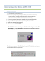
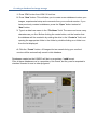
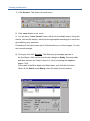
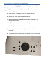
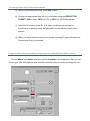
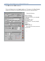
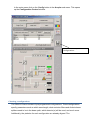
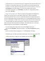
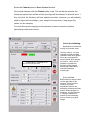
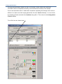
Zeiss LSM 510 Meta
Durham University
School of Biological &Biomedical Science
Centre for Molecular Imaging
[Type text]
Table of Contents
Turning on the system ................................................................................................................................ 3
Creating a database for image storage....................................................................................................... 4
Turning on the lasers .................................................................................................................................. 5
To view specimen in the transmitted mode, e.g. bright field .................................................................... 6
To view specimen in the fluorescence mode . ........................................................................................... 7
Using the Zeiss software to safely change objectives and reflectors (Filter cubes). .................................. 7
Acquiring a confocal image of your sample with the Lasers ...................................................................... 8
Choosing a configuration: ........................................................................................................................... 9
Single Track vs. Multi Track ...................................................................................................................... 10
Image optimisation ................................................................................................................................... 13
Acquiring your final image ........................................................................................................................ 15
Notes on image optimisation ................................................................................................................... 16
Zooming .................................................................................................................................................... 18
Z Sectioning............................................................................................................................................... 20
Time series ................................................................................................................................................ 22
Finishing up / Shutting down .................................................................................................................... 24
Opening your images offline .................................................................................................................... 26
Image Processing & Analysis .................................................................................................................... 27
Scalebars & Measurements .............................................................................................................. 27
3-D stack display options .................................................................................................................. 28
3-D Projection ................................................................................................................................... 29
Exporting Files to .tif Format ............................................................................................................ 29
Image formats................................................................................................................................... 30
Image window menu ................................................................................................................................ 31
Colocalization measurements .............................................................................................................. 35
Meta detector ........................................................................................................................................... 38
Lambda mode ................................................................................................................................... 38
Linear unmixing ................................................................................................................................ 38
Online fingerprinting........................................................................................................................ 39
Operating the Zeiss LSM 510
Turning on the system
1. Press Remote Control switch to on.
2. Turn mercury lamp on by pressing the black power switch on the Lamp
Control housing. The lamp should ignite within a few seconds allow
a five minute warm up. Make note of lamp hours in user log.
3. Turn on the computer as normal, Windows 2000 will load automatically.
4. Log on to Windows by simultaneously clicking Ctrl, Alt, and Del.
5. Enter your Username and Password.
6. Double click the LSM 510 META icon.
The LSM 510 switchboards will appear. Click Scan New Images and then Start
Expert Mode. If Scan New Images is not pressed, the software will start but
will not initialize the hardware.
The Main menu opens up. The LSM will go through a CP initialization and open a
tool bar labeled LSM 510 expert mode.
Creating a database for image storage
1. Press “File” button from LSM 510 tool bar.
2. Press “New” button. This will allow you to create a new database to store your
images, experimental setup and comments from your confocal session. If you
have previously created a database, press the “Open” button instead of
“New” button.
3. Type in a data base name in the “File Name” field. The name can be as many
characters as you like. Before clicking the create button, set the location that
the database will be created in by setting the drive in the “Create in” field, and
opening the appropriate folder in the folder by double-clicking on a folder icon
from the list displayed.
4. Click the “Create” button. All images that are saved during your confocal
session will be automatically saved in this database.
Databases created on the LSM510 will be in a proprietary *.mdb format.
Files in these databases are in a proprietary .lsm format, but they can be exported to
standard formats for use in other programs.
.
Turning on the lasers
1. Click Acquire. This opens up a sub menu.
2. Click Laser button in sub menu.
3. You will see a “Laser Control” menu with a list of available lasers. Using the
mouse, click on the laser(s), which has the appropriate wavelength to excite the
dyes labeling your specimen.
Preferably let the lasers warm up for 30mins before you collect images, 15 mins
are normally enough.
4. For Argon, first click Standby. The Warming up message appears in
the line Status. After a short time this will change to Ready. Now press On
and then increase the Tube Current to 6.1A by increasing the output to
approx 50%.
In the case of the Blue diode and HeNe lasers, just click the On button.
When all the Status reads Ready, close the Laser Control window.
To view specimen in the transmitted mode, e.g. bright field
Change the microscope-light path to direct the emitted fluorescence is sent to the
eyepieces by clicking on the ACQUIRE on the main menu then VIS in submenu. To
change the specimen raise the head, load your slide, cover slip down, add oil to your slide
before loading, lower the head. Then change to the desired objective, then raise the
stage, in that order. It is best to start with the 10x objective raise the stage and find focus
, this will prevent damaging very expensive oil lenses.
a) Set the Reflector Turret position to 1.(No filter set in the light path)
b) Press the HAL button( on left hand side of microscope).
c) Place your specimen on the stage, with oil if necessary, it should go on the
stage coverslip side down.
d) For Phase contrast match the condenser with the objective.
e) Adjust the light intensity as needed.
f) Focus using the course and fine focusing knobs on either side of the
microscope.
g) The motorised specimen stage is moved with either the joystick or round wheel
for fine movement
To view specimen in the fluorescence mode .
a) Switch of the transmitted light, press HAL button.
b) Choose the appropriate filter set for your sample using the REFLECTOR
TURRET. FS2 for Dapi, FS10 for FITC or FS15 for TRITC/Rhodamine.
c) Open the UV source, press FL. If all these conditions are met and no
fluorescence is present check the light path from the Mercury lamp to the
sample.
d) When you have finished viewing your sample pressing FL again will block the
fluorescence from your sample.
Using the Zeiss software to safely change objectives and reflectors (Filter cubes).
Choose Micro from Aquire submenu and the Axioplan Control appears, then you can
choose your filter and objective and have the computer raise and lower the stage for you.
Acquiring a confocal image of your sample with the Lasers
For LSM mode click LSM in submenu
Click on the Scan button in the Acquire sub menu. This opens up the Scan Control
window this will allow you to specify parameters and execute image acquisition.
Check the following:
Mode is selected
Frame is selected
Frame size X=512 Y=512 (CAN BE
LARGER)
Scan Speed = 6 or 7
Data depth = 8 Bit
Scan Direction = one way (straight
arrow)
Zoom = 1
Rotation = 0
Offset = centered
More details about these parameters
are given later
[
In the main menu click on the Config button in the Acquire sub menu. This opens
up the Configuration Control window.
Click here to open Track
Configurations
[
Choosing a configuration:
The LSM 510 has a number of pre-programmed configurations. These configurations
specify parameters such as which wavelength, what emission filters and dichroic beam
splitters need to be in the beam path, which detector(s) will be used, and much more.
Additionally, the pinholes for each configuration are already aligned. The
configurations are very convenient shortcuts. Configurations are selected based on the
fluorophore or fluorophors being used. If the excitation and emission spectra for the
fluorophore is known, chose the configuration that most closely matches it. (There is a
dye database in the LSM software. For a list of the excitation and emission
wavelengths of the fluors, go to OPTIONS on the LSM 510 - Expert Mode window,
then click on DYE DB .)
Single Track vs. Multi Track: There are 2 types of pre-programmed configurations:
Single Track and Multi Track. In most cases, Single Track is used for single-label
experiments and Multi Track is used for multiple-label experiments. Single Track can be
used for multiple labels as well as single labels, but it is recommended that Multi Track be
used for multiple labels. In Single Track, the system excites both channels simultaneously,
i.e., the wavelengths are scanned concurrently. In Multi Track, the system collects the
data sequentially, switching between wavelengths. This means that you can eliminate
bleed through from a second channel in multiple labelling.
For multi tracking with multiple labels choose Multi Track in the top row.
Now click the Config Box. (See previous figure) The Track Configuration window
appears.
Scroll to select the desired configuration, i.e. Fitc/Rhodamine. Click Apply.
Alternatively, you can open a previously stored image. In the main menu, select FILE
/ OPEN, then open an image from your database and click REUSE
.
Select the Channel panel in Scan Control window.
Set pinhole diameter with the Pinhole slider scale. The smaller the pinhole, the
thinner the optical slice will be and the less light will be collected. A pinhole set to 1
Airy unit (click the 1 button) will have optimal resolution. However, you will probably
need to adjust this according to your sample’s fluorescence, using larger Airy
values for dim samples.
For multi-fluorophore imaging set the pinholes for each channel to produce
equivalently thick optical slices.
Check the following:
Remember to select and
modify all channels used.
Pinhole adjust, remember to do
this for all channels used.
Set Airy units to 1 on one
channel and with multiple
channels make sure optical
slices are equivalent for
each channel while staying
as close to 1 Airy unit as
possible. Increase the
pinholes of the longest
wavelength channels to
match the shortest
wavelength.
Press the Fast
XY(Continuous scan) button
on the right side of the
window. This will start a
continuous image
acquisition that can be
halted by selecting the Stop
button. While the laser is
scanning, use the Remote
XY Stage Controller to
search for an interesting
area or frame up a good
image
Click on the New then Find button the right side of the Scan Control window. An XY-image
automatically adjusted for brightness and contrast is produced in the Image window. The
image will act a starting point for determining optimal settings
A specimen with 2 or more channels maybe easier to view with a split screen where each channel is
arranged side by side and the combined channel placed last.
Click the Split xy button located on the right side of the image window.
To enlarge the image window click the Zoom button then the In button in the right hand
column. The image will then fill one monitor screen completely. So pull the image over to the
Right hand monitor then zoom in.
Image optimisation
The pre-scanned image, whether too dim or too bright, usually needs to be optimized.
The PMTs need to be adjusted according to the fluorescence intensity of the sample.
Due to the sequential nature of „Multi-track‟ acquisition optimizing the settings in this mode is
difficult. It is easier to set the imaging parameters for each Track individually. You can do this
by switching off each track with the checkbox along side it. This is done in the Configuration
Control window.
Turn off all but one channel now.
You need to set the detector range to match the dimmest and brightest signal
from the specimen (set the full dynamic range of the image). Setting the detectors
incorrectly results in the loss of information from the specimen.
In the image window press the Palette button and highlight Range Indicator. This will
produce a monochrome image in the different channels for which the pixels with
intensity of 0 are blue and pixels with intensity of 255 are displayed red and assist you
in making the adjustments described below.
Start Fast XY and focus to the area of interest. The sample can be centred in the field
of view while the laser is scanning, use the Remote XY Stage Controller to search for
an interesting area or frame up a good image. When preparing for a Z stack it is
important to manually focus through the specimen's region of interest to find the
brightest focal planes and make the final adjustments to the detector based on them. It
will also be better to remove any averaging at this point.
Clicking Stop in the Scan Control window will turn off the Fast XY continuous
scanning.
Now start scanning again using Continous scanning.
Set Detector Gain and Excitation power –
The „max‟ signal is set by adjusting the detector gain and laser transmission
simultaneously. Adjust % laser transmission(s) in the Excitation Of Track panel at the
bottom of the window to the following guidelines. Doing so sets the % laser power let
through by the AOTF. 405 ~20%, 488 ~ 10-25% 514 >50%, 543 100%, 633 100%.
You need to empirically work out the best laser power settings – low laser power
causes less bleaching but requires the detector gain to be set high; which introduces
noise and may, if set to above 900, introduce background autofluorescence in that
channel. Set the Detector Gain until about 10% or less of your the brightest stained
areas have red pixel. In the case of a z stack it is better to have only a very few red
pixels.
Next move the Amplitude Offset until the background is no more than 50% speckled
with blue pixels. Clicking the arrows instead of the slider will make it easier to adjust.
If you are viewing multichannels remember do this for all channels used by switching
tracks on and off.
Reset the Palette to No Palette.
Acquiring your final image
Once you are satisfied that each channels detector is set optimally to the range of
the image, you can create your final image. Ensure that all Tracks are checked
when acquiring the final image.
Go to the Scan control window and click the Mode button.
Under Objective Lens & Image Size, choose a Frame size using the buttons
provided or you could choose the Optimal button
Noise can be reduced by averaging your final image, choose between line (default) or
frame averaging, using the mean (default) or summed intensity of 1,2,4,8, or 16 scans.
The amount of averaging necessary to obtain a good image depends on the signal to
noise ratio of your sample image. Low contrast images will require more averaging but
be aware that this could cause photobleaching. You can determine the amount of
averaging necessary to yield the best image of your sample empirically. As a rough
guide, averaging should be set to 100th the gain value, so meaning most samples will
require averaging of 4 or 8.
Scan speed: 6
The default scan speed (when not zoomed in) is 9. Reducing the scan speed can
improve a noisy image; faster scan speeds are used to find
regions of interest (like during the Fast XY function) or when photobleaching of
the sample is a concern.
The zoom and scan field rotation can be set in the Zoom, Rotation, & Offset
panel. You may find it more convenient to use the crop function in the Image
window - see the section titled Crop your image for details. Offset here refers to
fine XY movement of the laser.
When you’re “lost” with regards to magnification and offset, you’ll want to reset the field
view parameters. Go to the Zoom, Rotation, & Offset area at the bottom of the Mode
panel. Clicking the Reset button at the bottom right will take things back out to the original
magnification and offset settings
When image optimization has been achieved click on the 1/1 start scan button to
generate a single image of the specimen.
To save your image click the “Save” or Save As” button on the right side of the image.
This should default to our folder and to the database you have set up. In the Name
field, type a name for your image. Further information can be appended to this
database entry in the Description and/or Notes fields.
Notes on image optimisation
To reduce photobleaching attenuate the laser illumination by clicking the Channels
button in the Scan Control window. Under Excitation of Track you can reduce the
percentage of laser power (Transmission %) for each excitation wavelength. If this is
necessary you may need to compensate by readjusting the sensitivity of the detector
as described above.
To further improve image quality you can slow down the scan rate or apply averaging
to remove random noise, sum to increase signal, or choose a combination of these.
Also, you may increase frame size to higher than 512 x 512 by selecting Mode on the
Scan Control and changing the resolution.
512X512 is good for large stacks 50um + or for high n statistical requirements. Fast
scanning of stacks, 3.9 seconds a slice, line average of 2 required to remove
pixelation.
1024X1024 is good for small stacks 25um and lower or for low n statistical
requirements. Average scanning 15 seconds a slice, optional line average of 2
required to remove noise. May not need to be averaged at all. Good for zooming in
and cropping
2048X2048 is great for publication quality covers, slow scanning 15seconds to 1minute
a slice averaging not required but may be applied.
To change the frame size click the button with the desired frame size. Going to larger
frame size will concomitantly increase both the size of the file and time to acquire the
stack.
You can adjust the area to be scanned by using the options found in: Zoom, Rotation &
Offset under Mode or by using the crop tool.
Changing the scan resolution or scan speed will change the image histogram so the
Channels settings should be readjusted.
Line Switching vs. Frame Switching: In Multi Track, there is a choice between Line
switching or Frame switching. In other words, you may select whether you want the
system to switch tracks after each line or each frame. In Line switching mode, the
system scans line by line, switching tracks sequentially. For example, if the first line is
A®B and the second line is C®D, the system will scan A®B with Laser 1, then scan
the same line with Laser 2, then scan C®D with Laser 1, etc. [Note: This is if the
system is set for unidirectional scanning (see page 10). In bi-directional scanning, the
system would scan A®B with Laser 1, then B®A with Laser 2, then C®D with Laser 1,
etc.]
In Frame switching, the system scans the entire X-Y plane with Laser 1, then goes
back to the start and scans the X-Y plane with Laser 2.
Line switching vs. Frame switching: In Line mode, you cannot change dichroic
filters between scans, because there is not enough time at the end of the row. In
Frame switching, you can change dichroic filters between scans, so there may be
occasions when you need to use frame switching to acquire a difficult image. Frame
switching is not a good choice for kinetics, however, as there is such a time lag
between the 2 collections (i.e., before the same pixel is scanned the second time).
Zooming
This function is a true zoom performed upon image acquisition - the laser will scan a
user-defined region of interest and display the scan data in a user-defined frame size
(512x512, etc).
1. Select Crop from the image window‟s Display toolbar. A crop box appears in the
current image window. Move the mouse over the crop box to change the zoom, offset,
and rotation of the cropped scan.
2. To set the offset, position the mouse inside the crop box. The cursor will change
to an icon of perpendicular arrows indicating direction in the X and Y dimensions.
Use the left mouse button to drag and drop the crop box to the desired offset
position.
3. To set the zoom of the scan, position the mouse over a corner of the crop box.
The cursor will change to an icon indicating zoom in/out relative to a centerpoint.
Left-click and drag until the desired zoom has been achieved. Release the
mouse button at this time.
4. To rotate the scan, left-click on an end of the crosshairs and drag to set your
desired rotation. The cursor will change to a circular icon indicating rotation
around a centerpoint. The blue side of the crop box indicates the top of the new
cropped scan that will be acquired. Release the mouse button once you‟ve
achieved the desired rotation.
5. To make your image frame rectangular, left-click on any of the intersections
between the crosshair and sides of the square. The cursor will change to
up/down or side-to-side arrowheads, depending on the dimension you want to
change. That side can then be dragged and dropped to the desired frame size.
Z Sectioning
Once you have set up your image as defined in the above section, you can
collect a series of confocal images through all or any of the focal planes of your
specimen. To collect a series of images at different points along the z-axis the settings
can be inputted in two ways: Z Sectioning or Mark First/Last.
Z-sectioning – takes x slices at a particular z interval and assumes the user has prior
knowledge of the specimen’s thickness and/or is willing to guesstimate thickness.
Mark first/last – the operator sets the top and bottom of the sample and selects either
the interval or number of slices (the other is calculated for you).
Details for Mark First /Mark last
You may set the number of slices or the interval depth. Start by first determining the
total volume to scan.
.
1. Press the “Z Stack” button on the “Scan Control” menu this activates the Z Settings
panel.
2. If you have slowed the scan rate or have set image averaging, it is a good idea to
temporarily resume fast scanning to find the lowest and highest points of focus. Do this
by clicking on “Fast XY” Also you will find it easier when multi-tracking to uncheck all
but one of the channels, as you did when setting channel parameters.
3. Click on Mark first /Mark last slice.
4. Click the “XY cont” button to start scanning and determine the start and end points
of the Z stack. Z sectioning is usually performed moving into the specimen; away from
the coverslip. However starting deep reduces photo bleaching at the dimmest point. To
find the starting point for the Z stack focus toward the coverslip (rotate fine focus knob
toward you) until you reach the point at which you‟d like to begin the Z stack.
5. Click “Mark First” button to set upper position of Z-stack
6. Focus through specimen until you find the last image of your Z-stack
7. Click “Mark Last” button
8. Click Stop button to end continuous scanning
9. Assuming you have already adjusted your pinholes as described on page 9 look up
the optimal z interval thickness by clicking Z Slice at the top of the Z Settings box.
This will open the Optimal Slice window. Optimal z interval thickness for the objective
currently in use will be displayed in this window. Clicking Optimal Interval in the lower
left corner of the window will set the z interval of your z stack to the recommended
thickness. (note: optimal interval will most likely change the number of slices you are
taking. Be sure to check this and take smaller number of slices if appropriate.)
10. For 3D reconstructions press x:y:z=1:1:1 this ensures cubic pixels and no
stretching or squashing of the image will occur.
11. Remember to check all Tracks again and reset any averaging.
12. Press 1/1 and the Z stack will be collected.
13. The collected z stack is temporarily stored in the computer‟s memory. To
permanently store the stack, use Save or Save As in the image display window
to save it to your database.
Time series
The Time Series is a versatile software function that is useful in a variety of
situations – from collecting single confocal images or entire z stacks over time to more
sophisticated applications such as FRAP. If desired, a delay between the beginning of
one scan process to the beginning of the next can be set. It is important to note that
Time Series works at only one location on the slide. To apply the Time Series function
to multiple stage locations, you will have to use the Multitime macro.
The following instructions are for applying a basic Time Series. It is assumed that
the user has optimized and set all imaging parameters beforehand (pinhole size,
detector gain/offset, scan time, averaging, and if desired, z stack).
1. Select the Acquire_ Time Series submenu.
2. In the Start Series panel, choose between a Manual start or a timed start via
Time. Most users want a manual start. If a timed start is desired, enter a start
time in the Time (h:m:s) field. The time series will start when the set time is
reached according to the computer‟s clock.
3. In the End Series panel, enter the number of time points desired in the Number
field if a Manual end is selected. For a timed end point, depress Time and enter
the end time in the Time (h:m:s) field.
In determining an experiment’s length and the number of time points needed it is
important to consider the scan time and averaging settings (see the Speed section of
the Mode panel in “Scan Control”). Both parameters influence how long it takes the
laser to clear the scan field and thereby define the minimum time between time points.
4. The next panel you encounter will be either Time Interval or Time Delay,
depending on the settings of your Time Series register (see Options_
Settings). Time Delay is defined as the end of one scan process to the
beginning of the next, while Time Interval is the time between the beginning of
one scan process to the beginning of the next. Either panel, Time Interval or
Time Delay, permits time series scan parameters to be activated or changed
from experiment to experiment.
You may load & Apply previously saved time series settings using the
pulldown menu in either of these panels. Or you may choose to manually enter
scan parameters into the Time and Unit fields. If you foresee performing other
experiments with identical time scan settings, you should Store your manually
entered settings to the dropdown list for easy reference in the future.
5. Click Start T in the right-hand side of the Time Series window to start your time
series.
6. The collected time series is temporarily stored in the computer‟s memory. To
permanently store the series, use Save or Save As in the image display window
to save it to a database.
Finishing up / Shutting down
If another user is following you in then all you need to do is to log off the computer and
clean up as outlined below.
Select Argon/2 laser unit
Set Argon/2 laser Output (%) to minimum (25%)
Switch to stand by
If another user is arriving within the next two hours (see booking page) the lasers
may be left running
If another user is not arriving ensure that all lasers are powered Off
The last user of the day who is booked is responsible for ensuring that system is
shutdown. If you have cancelled on the same day then:
Contact previous user, or
Call the facility to ensure system has been shut down, or
Come over to facility to ensure system is shut down yourself.
Laser fans will run for about 5 minutes then turn off automatically (a reduction in
noise will be heard)
Clean up immersion lenses used with lens tissue only
o
Blot glass lens element
o
Rub metal barrel
Clean up oil and fluids from stage
Exit Zeiss software
Transfer data to e.g. burn CD, etc.
Once laser fans have become quiet (automatically powered down) turn Remote
Control switch off. Switching of before the lasers are cool will seriously damage
them.
Switch off Mercury Arc lamp and sign the daily usage record sheet.
Log off from the computer and shut it down.
Replace microscope dust cover.
Put all used disposable paper products, cans, wrappers, etc. into trash can
It is your responsibility to back up your files and then delete them from the hard
drive. It is assumed that all images are backed up and if disc space is required I will
delete images to make space!!!!
Opening your images offline
Zeiss image browser
http://www.zeiss.de/lsm
Follow link in lower right hand corner:
“Free LSM Image Browser”
Requires a registration form to be completed and also the download and
installation of an extra DAO file if you have Microsoft Office 2000.
ImageJ
http://rsb.info.nih.gov/ij/
Plus Zeiss plugin
http://rsb.info.nih.gov/ij/plugins/lsm-reader.html
Requires LSM images to be saved “uncompressed”.
WCIF ImageJ is a bundle of plugins along with the core ImageJ files. This can be
freelydownloaded from the WCIF website downloads section
http://www.uhnresearch.ca/wcif.
It is highly recommended that you copy your entire database ( Complete folder)
and keep this raw data as it carries with it all of the acquisition data which is lost
when images are exported.!
Image Processing & Analysis
Scalebars & Measurements
A scale bar, measurements (e.g. angle, area, line) and/or text can easily be drawn
onto an image that has already been collected using the Overlay option in the image
display window. You are encouraged to explore the drawing buttons in the Overlay
toolbar – creating a scalebar on your image is described here.
1. Click Overlay in the Select toolbar of an open image window.
2. Select the desired scalebar thickness from the line width option buttons
appearing half way down the Overlay image window submenu.
3. Click on the desired color of your scale bar from the color selection at the bottom
of the Overlay submenu.
4. Click 1μm in the Overlay submenu, then click in the vicinity of the image where
you wish the scalebar to be drawn.
5. Drag the mouse over some distance on the image until the resulting scalebar
registers your desired value. Release the mouse button to draw this scalebar
overlay on the image.
6. Use Save or Save As in the image window to save it to a database.
3-D stack display options
Animate
Some users will find it helpful to assess their time or z-stack data by animating it.
1. Select Anim from the Select toolbar of a stack‟s image window. The Animate
window will open and the stack will immediately be animated.
2. Speed 1 and Speed 2 in the bottom section of the Animate window allow the
user to control the speed of the animation.
3. To further control the animation, use the function buttons in the top section of this
window to animate forward and/or in reverse, stop, fast forward, and fast back
through a stack. + and - will animate the stack in forward or reverse by
whatever increment you choose in the Increment slider in the bottom section of
this window.
4. The Increment slider reduces the number of slices included in the animation to
every nth slice as selected.
Gallery
Stack slices are organized in rows and presented in the order in which they were
generated inside the image window. A 2-dimensional gallery of z-stacks over time can
also be generated. Each slice‟s z-data (μm) and/or temporal interval can easily be
displayed in every tile of the gallery. Z- or t-galleries can be saved as an image in a
database for quick future reference. Additionally, a subset of images within a stack can
be selected and stored for later use (e.g. to create a 3-D projection).
1. Click Gallery in the Display toolbar of the image window. A gallery of the entire
stack is automatically generated and the Gallery toolbar becomes available in the
image window. Click Save if you want to save the gallery to your database for
quick future reference. Otherwise, a gallery view can always be generated from
the stack at a later time.
2. For z-stacks taken over a time series, refer to the Gallery menu to select the
format in which you‟d like the gallery be displayed – Z , Time , or entire z-stacks
over time, Z + Time .
3. To have the stack data (z distance or time interval) displayed in every tile of the
gallery, click Data in the Gallery toolbar. Use the color selection button (located
below Data ) to ascribe a color of your choice to the gallery data display.
4. To separate a subset of images from the full image gallery, select Subset in the
Gallery toolbar. Here, define new start and end points of the series using the
Start Slice and End Slice sliders/data fields, or enter a value in the Every n-th
Slice field if you would rather create a subset of every n-th slice of your
choosing.
3-D Projection
The Projection function can render a single projection or a series of calculated
projections at set angle increments around the X, Y, or Z axis. The user can choose
between manipulating aspects of the projection‟s transparency or creating a projection
that has maximum intensity.
The “Transparent” projection method decreases the brightness of each file in the
projected stack to reveal structure in subsequent layers that would otherwise be
hidden.
The “Maximum” projection method takes the intensity values of individual pixels in all
sections and collapses them into one single illuminated image. The “Maximum”
method is chosen when the maximum pixel intensity is desired to be represented in the
projection.
Creating a maximum projection is described here. These instructions assume that
an image stack is open and therefore available for projection
1. Select 3D View_ Projection from the main menu. The Projection window will
open.
2. Select the stack to be projected in the Source panel of this window.
Only stacks and images that are currently open are available for selection in the
Source pulldown list.
3. To create an en face (straight-on) projection of all slices in the z-axis, select the
Y radio button in the Projection panel. Leave the First Angle set to 0°, enter 1 in
the Number Projections field, and set the Difference Angle field to 0°.
4. In the Transparency tab, select the Maximum radio button.
5. Generate the projection by clicking Apply located in the upper right corner of the
Projection window.
The projection calculation can be monitored via the progress toolbar at the bottom of
the image window.
6. If a sequence of projections at set angles has been created, it may be animated
or viewed in a gallery via the Select and Display toolbars of the image window.
Exporting Files to .tif Format
Files can be exported in a couple of different ways – via the batch export macro,
which allows the simultaneous export of multiple database items or the Export of
Images function, which allows the export of individual database items – be they single
confocal sections or a stack. The Export of Images method is described here.
1. Open your database and load (open) the file you would like to export.
2. Select File_ Export from the main menu. The Export Images and Data window
will open.
3. In the Save In field, designate to which drive or directory the exported data
should be saved.
4. Enter a name for the exported image or series of images in the File name field.
5. In the Save as type field, select the image format into which the file should be
Exported.
When selecting an image format, pay heed to whether you are exporting a single
confocal
image or a series (stack) of confocal images. Various image formats are supported
(e.g. .bmp,
.jpg), we recommend TIF (.tif) format as it is lossless and widely usable.
For multi-channel images, you have the option of exporting individual color channels of
data in monochrome (grayscale) if Raw data single or Raw data series image type is
chosen.
6. Click Save. When a z- or time stack file is exported, each stack slice is stored as an
individual TIF image
with a 3-digit numbered suffix appended to the designated file name.
Image formats
In the Export Images and Data window, you have several options how to export your
images (Single option is for a single image, Series is for a Zstack):
Raw Data Single/Series: Use if you want to control the separation of labels into
different RGB channels (e.g. if you want to have green channel as an own image file).
Exports only the original scanned data, i.e. brightness/contrast or pseudocolor
changes are not applied to the exported image. Also, no overlay information is shown
in a raw data image. This is the choice if you are going to analyze your image. Note
that an image can only have three different channels (RGB), so if you have taken an
image with four fluorochromes, you will have to export two images (one with three
channels and another with one channel).
Contents of Image Window Single/Series: Image resolution is not determined by the
frame size selected for scanning but by the image window size on the screen. Because
the resolution may change when this option is used, it is not recommended.
Full Resolution Image Window Single/Series: Exports a full resolution
image as determined by the frame size before scan (in contrast to the “Contents of
Image Window single” option). No control over channels as in “Raw data single/series“.
Will include scale bars and other overlays. Changes made in the image after scanning
e.g. brightness/contrast or pseudocolor changes) are also included so be aware that
even if you took care not to have any saturated pixels in your original scanned
image,you can still create saturated pixels by making post-acquisition changes. Those
changes will remain in the image, if you use this exporting option.
Image window menu
All image window tools can be closed by pressing the corresponding button again.
Depending on your current image (single/multichannel/Z stack etc.), some tools may
not be active.
CHAN
Clicking on the CHAN shows the Channels toolbar. When you click on a channel
button in this toolbar, you can then either turn off the selected channel by clicking the
OFF button, or change the pseudocolor used for that channel by clicking on another
color.
More color selection buttons can be created by pressing COLORS button. First define
the hue of the new color in the larger window, and then select the saturation of the
color by moving the arrow along the smaller window. Clicking the ADD button adds
the new color button in the color selection window.
ZOOM
Zooms the image (does not affect scanning); after clicking on the ZOOM button,
ZOOM toolbar becomes visible. ZOOMAUTO:
Automatically fits the image to the
size of the Image window. ZOOMRESIZE
and ZOOM 1:1: both restore the image
into its original size. ZOOM+:
Enlarges the image 200%. ZOOM:
Reduces the
image into half of its original size. ZOOMMOUSE:
After selecting this button, the
left mouse button can be used for enlarging the image, the right button for reducing
the size (cursor has to be over the image). The underlined functions can only be used
when ZOOMAUTO
is inactive. The zoom factor can also be adjusted by using the
slider. The display box shows the zoom factor.
SLICE
Used for viewing individual images of a Z stack or time series. By dragging the slider,
you can view the images one by one. The display box shows the number of the current
image and the total number of images.
OVERLAY
By pressing OVERLAY, overlay toolbar becomes visible. SCALE button (1
micrometer scale bar shown in the button) allows you to draw a scale bar in your
image. You can change the color of the selected scale bar by clicking on one of the
color boxes. The length of the selected scale bar is adjusted by dragging.
You can measure area and lengths of objects drawn in the image: first draw an object
using the drawing tools. Then select the object by clicking on it, and also click on the
MEASURE tool (yellow ruler in the button). Depending on the object, either its
lenght or area will be shown.
OFF removes the selected object; the button becomes ON, and clicking it again will
show the object again. RECYCLE BIN tool deletes the selected object. Is is also
possible to drag objects into the RECYCLE BIN if you want to delete them.
CONTR
Changes the contrast and/or brightness either for each channel separately or all
channels simultaneously. Usually not a very useful feature, as the settings are
automatically optimized by the software. By clicking MORE, you can also adjust
gamma; just remember that this adjustment should be described in your manuscript.
PALETTE
Pseudocolor palettes can be selected: RANGE INDICATOR is useful for determining
the settings for DETECTOR GAIN and AMPLIFIER OFFSET. RAINBOW can be
used for indicating intensity values using a color scale instead of a brightness scale.
GLOW SCALE is a combination of color and intensity scales.
ANIM
Animation of frames of a Z stack or time series.
Speed 1: very fast; speed 2: slower.
REUSE
Allows you to load acquisition parameters of the selected image, provided that the
image is in LSM format in an MDB database.
CROP
Defines the zoom area for scanning (see chapter 6.1.4).
COPY
Copies the current image into the clipboard.
SAVE
Saves the current image into an MDB database without showing the dialog window.
SAVE AS
Saves the current image, shows a dialog window in which you can select the database
and name the image.
XY
Displays a single image; multiple channels are in superimposed mode.
SPLIT XY
Shows channels in separate windows; the last window shows the superimposed mode.
ORTHO
Shows an orthogonal view (= xy, xz, and yz planes of Z stacks). XY plane is in blue,
XZ in green, and YZ in red. The section plane can be positioned at any XYZ
coordinate of the Z stack by moving the sliders in the Orthogonal toolbar.
Alternatively, the number of the slice can be entered in the input box.
By clicking on the DIST button it is possible to measure distance in 3D: Click on
MARK button to define the first XYZ point. Set the second point by either moving
the X,Y,and Zslidersor the green, red, and blue lines in the image. The distance
between the two points is shown in micrometers at the bottom of the Orthogonal
toolbar. The projections of the spatial distances are shown in yellow in the image.
2D DVC button can be used for 2D deconvolution, which improves the axial (Z)
resolution.
CUT
From a Z stack volume, you can select a section plane, which can be of any
orientation, and the CUT function will create the corresponding Z stack. Clicking on
CUT will show the Cut toolbar. The cut plane is determined by adjusting the X,Y,Z,
Pitch,and Yaw sliders.
The selected cut plane is shown in red at the bottom of the Cut toolbar, as well as in
the image window.RESET ALL restores the original settings. TRILINEAR
INTERPOLATION improves the image quality by applying 3D interpolation.
GALLERY
Displays all images of a Z stack, lambda stack, time series, or their combination side
by side. In the Gallery toolbar, clicking on the DATA button shows either the Z slice
distance, wavelength, time, or their combination, whichever is relevant. COLOR
button allows you to change the pseudocolor for all images at the same time. Clicking
on SUBSET, the Subset window opens, enabling you to select only a subset of the
images: select the START SLICE and END SLICE for the new subset by dragging
the sliders. Be aware that when you click on the OK button, the slices not included in
the new subset will be permanently lost.
HISTO
Displays a histogram (distribution of pixel intensities) of an image, gives size and
intensity measurements for a given area, as well as analyzes colocalization between
two channels.
Histogram
In the histogram toolbar, the following functions are for the histogram display:
SKIP BLACK: Pixels that have the gray (intensity) value of zero are not shown in
the histogram
SKIP 4%: Pixels that have the lowest 4% of the gray (intensity) values are not
shown in the histogram
SKIP WHITE: Pixels that have the highest gray (intensity) value (255 for an 8bit
image and 4095 for a 12bit
image) are not shown in the histogram
STEP: Determines the number of intensity levels shown in the histogram. Step 1
corresponds to 256 intensity levels for an 8bit
image, step 64 to 256/64 = 4
intensity levels
SHOW IMAGE: Shows the image window next to the histogram
SHOW TABLE: Shows the numerical values of the histogram in a table
COPY TABLE: Copies the histogram table into the clipboard
SAVE TABLE: Saves the histogram table as a text file (.txt)
Area measurements
In the histogram toolbar, the following functions are for the area measurements:
AREA: Used for defining the area for size and intensity measurements by using
the Area tools at the bottom of the histogram toolbar. First, define the area using
the drawing tools. Then, make the necessary adjustments for the area histogram
using the following tools:
STEP: Determines the number of intensity levels shown in the area histogram.
Step 1 corresponds to 256 intensity levels for an 8bit image, step 64 to 256/64 = 4
intensity levels
LOW: Sets the threshold intensity level; pixels with lower gray values than the
threshold value are masked with the color selected using the COLOR selection
button below the low threshold value box.
HIGH: Pixels with higher gray values than the threshold value are masked
with the color selected using the COLOR selection button below the
high threshold value box
Mean intensity value, standard deviation of the intensity, and the size of the
nonmasked area are shown below the COLOR selection buttons.
Instead of defining the range of intensity values for area measurements, you can
also use the Mask tools for masking areas masked pixels are not included in
measurements:
MASK: Enables the Mask mode, in which masked areas can be defined by ink
FLOOD FILL: Fills the defined area with the color selected under MASK
COLOR SELECTION: Defines the color of a mask
CLEAR MASK: Removes the mask color
Colocalization measurements
In the histogram toolbar, the following functions are for the colocalization
measurements:
COLOCALIZATION: Shows a scatter plot in which the X coordinate of the pixel
Px presents the intensity value of that pixel in channel 1, and the Y coordinate
presents the intensity value of Px in channel 2. If there is complete colocalization
between the channels, the scatter plot should show a diagonal line from the bottom
left corner to the top right corner.
SHOW TABLE: Shows the numerical values of the scatter plot in a table
AREA: Shows the image window next to the scatter plot
CROSSHAIR: Displays movable crosshair that, when correctly adjusted, divides
the scatter plot into four regions: bottom left region: background intensities;
bottom right region: pixels that have intensity values above threshold only in
channel 1; top left region: pixels that have intensity values above threshold only in
channel 2; top right region: pixels that have intensity values above threshold both
in channel 1 and 2.
Note that because there are no stringent criteria how to set the crosshair (threshold
values for each channel), this is always a somewhat arbitrary method.
THRESHOLD: SET FROM IMAGE ROIS: Sets background threshold from ROI
(region of interest) drawn in the image
INVERT MASK: Inverts the mask or scatter plot
SOURCE 1: Selection of channel 1 and its color via the Color box
SOURCE 2: Selection of channel 2 and its color via the Color box
MASK: Select either RGB or OVERLAY for the mask; selection of mask color
via the Color box
Drawing tools can be used for making ROIs in the scatter plot and image, which
are interactively linked (selecting a ROI in the image shows a scatter plot for those
pixels; selecting a ROI in scatter plot shows the corresponding pixels in the
image).
In the table, the following measurements are shown:
Number of pixels (in the whole image or ROI)
Area (in the whole image or ROI)
Mean intensities and SD (in the whole image or ROI)
Colocalization coefficients
Weighted colocalization coefficients
Manders' overlap coefficient
Pearson's correlation coefficient
Remember that overlap in distribution patterns does not indicate that the labeled
molecules interact with each other, or that their distribution patterns correlate with
each other.
PROFILE
Displays the intensity distribution for each channel along a line drawn on the image.
Also shows the numerical intensity values that can be saved. By using markers (red
and blue), you can measure intensity difference and distance between two points
along the line.
In the Profile toolbar, the following functions are available:
The drawing tools can be used for drawing either a straight or curved line along which
the intensity values will be shown. You can also select the thickness and color of the
line; these will not affect the measurements.
DIAGR. IN IMAGE: Shows the intensity diagram as an overlay on the image
MARKER 1 (red): Shows a red circle marker in the image, and a red line marker in
the intensity diagram
MARKER 2 (blue): Shows a blue circle marker in the image, and a blue line marker
in the intensity diagram
ZOOM: Zooms on the intensity diagram; click and drag a rectangle on the graph and
that area will be enlarged. Can be applied several times. Rightclick
will reset the original size
RESET ZOOM: Resets the zoomed intensity diagram into the original size
SHOW TABLE: Shows the numerical intensity values in a table
COPY TABLE: Copies the table into the clipboard
SAVE TABLE: Saves the table as a text file (.txt)
2.5D
Shows pseudo3D
intensity distribution for each channel. Handy for presentations.
For Z stacks, the slice selected using SLICE in the Image Window menu is displayed.
Scrollbars around the image are used for rotating the image around the horizontal and
vertical axes. The right scrollbar on the right side of the image controls the intensity
scale of the image.
In the Pseudo 3D toolbar, the following functions are available:
PROFILE: Vertical polygon display
GRID: Horizontal grid display
FILLED: Color display, in which MONO, RAINBOW, and SIX STEP options
CHANNEL: selection of the channel displayed in case of a multichannel image.
Prev
Composition of images, diagrams, tables, and text for printing. However, there is no
printer connected to the Meta computer.
Info
Displays the parameters that were used when the image was acquired. This
information will be stored together with the image in the MDB database. If you save
your image in TIFF format, none of this information will be stored, just the image.
Meta detector
META detector (ChS) is a spectral detector which means that you can freely select the
range of emission wavelengths that you want to use for detection. It consists of 32
photomultipliers, each of which covers a spectral range of 10.7 nm (total range about
340 nm)
Lambda mode
You may want to use META detector in case the emission filters available are not
optimal for your fluorochrome. Additionally, you will get the spectral emission
(intensity for each wavelenght within your selected range). When you scan in this so
called lambda mode, the result will be a lambda stack that shows the signal over the
spectral range selected. It is also possible to combine lambda mode with Z mode
and/or time series.
However, META detector is less sensitive compared to the other detectors, so you
should have a strong signal if you want to use the META detector. Also, you may
need to open the pinhole more than usually (try using e.g. 3 Airy units).
To use lambda mode, select LAMBDA MODE in the configuration control window.
Set the excitation and main dichroic beam splitter (HFT n) as in the CHANNEL
MODE. For selecting the detected wavelenghts, either use the slider or write the
starting/ending wavelengths in the proper input boxes. When you click on the
CONFIG button, you can save and load lambda configuration. NUMBER OF
PASSES will tell you how many scan are needed to cover the required spectral range.
Proceed to SCAN as usual.
For separation of spectral signals, you have two options: either LINEAR UNMIXING
or ONLINE FINGERPRINTING.
Linear unmixing
META detector and linear unmixing can be used to separate signals from two or more
fluorochromes with overlapping emission spectra. Also, autofluorescence can be
separated from the true signal.
In linear unmixing, the software will calculate for each pixel how much of the signal
is derived from each spectral component that needs to be separated from the others,
based on the reference spectrum for each component. In order to make a reference
spectrum, you need to have control specimen that are each stained with only one of
the fluorochromes whose spectra need to be separated. In case of autofluorescence,
the control is simply an unstained specimen.
LINEAR UNMIXING is used after you have acquired a Lambda stack (using META
detector). In the MAIN menu, select PROCESS, and then UNMIX. Insert in the stage
the specimen from which you want to acquire a reference spectrum. It is essential that
the specimen is only stained with the fluorochrome for which you want to get a
reference spectrum. Select the channel for the reference spectrum and name it. Press
the LOAD FROM IMAGE button. Continue until you have acquired reference spectra
for all the fluorochromes whose spectra you want to separate from each other.
In the Source panel of the UNMIX window, click on the arrow button and select the
image you want to use for unmixing by clicking on it. In the Parameters panel of the
UNMIX window, select all options. The RESIDUALS channel will show you the
amount of signal that could not be assigned for any of the unmix channels. ASK FOR
THE BACKGROUND ROI option will ask you to mark an area in the image that
represents background. This background channel should be defined for optimal linear
unmixing.
After clicking on APPLY, a new window that shows the result of the unmixing will
open.
Online fingerprinting
ONLINE FINGERPRINTING does the unmixing during scanning, and the lambda
stack will not be shown or stored. If you want to use this option, you must have saved
the reference spectra in the PROCESS/UNMIX window in advance (see previous
chapter). Select ONLINE FINGERPRINTING in CONFIGURATION CONTROL
window. Load the reference spectra using the RS1 ... 8 control buttons. Set the
excitation and main dichroic beam splitter (HFT n) as in the CHANNEL MODE. For
selecting the detected wavelenghts, either use the slider or write the starting/ending
wavelengths in the proper input boxes. When you click on the CONFIG button, you
can save and load configurations. NUMBER OF PASSES will tell you how many scan
are needed to cover the required spectral range. Proceed to SCAN as usual.