Download Agilent Technologies PN 8510-16 User`s guide

Agilent PN 8510-16
Controlling Test Port Output
Power Flatness
Product Note
UNCORR
ECTED P
OWER
CORREC
TED POW
ER
OUTPUT
Agilent 8510C Network Analyzer
POWER
Introduction
Designers and manufacturers of active devices
often need to control the power level at the test
port1 of their power-sensitive devices, but find difficulty in overcoming insertion losses. The insertion
losses occur as a result of connecting components
in the measurement path between the source and
the DUT. The Agilent Technologies 8510C is a
microwave network analyzer2 capable of setting
and controlling the power level at the test port.
This product note reviews the implementation
and operational considerations of the 8510C’s
test port power flatness-correction feature.
The 8510C performs a flatness-correction calibration by measuring the test port power level
using an Agilent power meter and creates a table
of power corrections versus frequency. The
power meter then stores the table into an Agilent
8360 series synthesized sweeper.3 When the test
port flatness correction is enabled, the source
will adjust its output power to compensate for
path losses at each measurement point in the
frequency span.
1. In this document, “test port” will refer to the point in the system where the test
device is connected. This may be port 1 or port 2 of any 8510 coaxial-based test
set or the end of a cable or adapter that is attached to the DUT.
2. 8510B network analyzers with revision B.06 or later may also be used to achieve
constant test port power levels. To obtain the latest firmware revision order the
11575F upgrade kit.
3. Any 8360 synthesized sweeper with firmware revision of September 25, 1990 or
earlier must be upgraded. To upgrade your 8360 to the latest firmware revision,
order part number 08360-60167.
2
Power flatness correction is useful for characterizing active devices by allowing measurements of
absolute power, gain versus input power, and
swept-frequency gain compression. Swept-power
gain compression measurements are possible in
the power domain with the flatness correction
enabled.
The 8510XF measurement system is capable of leveling and controlling the test port power between
45 MHz and 110 GHz without requiring a power
calibration for each measurement. When power leveling is enabled, the test port power variation is
typically less than ±1 dB over the full frequency
sweep, with 20 dB of adjustable power. For more
information regarding power leveling in the Agilent
8510XF, refer to product note 8510XF-1, literature
number 5968-5270E.
System Configuration
The basic 8510C measurement system configuration needed for test port flatness correction is
shown in Figure 1. A single channel power meter
such as the Agilent 437B, E4418A, or E4418B is
required, along with a compatible sensor, for performing the power flatness calibration. Power
meters with the 437B command set must be used
for the power level flatness correction.
The Agilent 8511B frequency converter test
set may be used with the test port power flatnesscorrection feature. The range of the test port
power is determined by the available power of
the 8360 source and the insertion loss of the components added to the measurement system.
85107B Measurement System
8510C network analyzer
8510 system bus
8517B test set
8485A
power sensor
E4418B
power meter
83651B
synthesized sweeper
Figure 1. Basic Agilent 85107B measurement system configuration for test port flatness correction
3
Flatness-Correction Operation
The basic setup procedure to obtain flat test port
output power is illustrated in Table 1. To simplify
the execution of the procedure, the front panel
hardkeys are enclosed in [brackets]. The softkeys
are enclosed in {braces}. Table 2 provides the procedure for setting up the power meter. The network analyzer should be reset before performing
any procedures. The flatness-correction calibration
can be performed in step, ramp, or frequency list
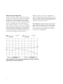
sweep mode. Figure 2 illustrates test port power
versus frequency with and without flatness correction using an 85107B measurement system.
When the flatness correction is enabled in an
8510C measurement system the analyzer’s Power
Source 1 softkey controls the test port power level.
The source and test set used will determine the
available test port power range.
The maximum leveled power the source can output at different frequency spans is indicated in
Table 3. Once the flatness correction is enabled,
the test port power level must be set within the
power range presented in Table 4 for common
source/test set combinations.
Figure 2. Comparison of test port power without flatness correction (channel 1)
and with flatness correction (channel 2)
4
Table 1. Flatness-correction calibration procedure
8510C Keystrokes
Description
Set up the power meter (see Table 2)
For proper operation, the E4418B must be set up before initiating the flatness-correction routine.
See Table 2 for specific instructions.
Verify the power meter's address on the 8510 system
[LOCAL]
When shipped from the factory, the address of the power meter is 13. If this conflicts with another instrument on the system bus,
{POWERMETER}
change the address of the conflicting instrument. The power meter must be set to address 13 in order for the firmware to function properly. Press [SYSTEM/INPUTS], {REMOTE INTERFACE} and {INTERFACE OVERVIEW} on the E4418B to ensure the
power meter’s address is set to 13. Verify that the power meter is connected to the system bus.
Set up the analyzer and measurement
Set up the start/stop frequencies and the measurement type (for example, S11, S12).
Adjust the number of analyzer trace points (if needed)
STIMULUS [MENU]
When the flatness calibration is initiated, the analyzer sends the source a list of flatness-correction frequencies equal to the
{NUMBER OF POINTS} number of trace points set on the analyzer.
{POINTS}
Set the source to the maximum leveled power
STIMULUS [MENU]
Set the 8360 for maximum specified power (P1) at the highest frequency in the span; see Table 3. At higher power levels, the
{POWER MENU}
power meter will take less time to settle between measurement points during the calibration process.
{POWER SOURCE 1}
P1 [x1]
Connect the power sensor to the active test port and begin the flatness calibration
Initiate flatness calibration
{POWER FLATNESS}
Do not cycle the power on the analyzer or the source during the calibration process. The calibration may be aborted at any time by
{CALIBRATE FLATNESS} pressing any key on the analyzer’s front panel. Aborting the calibration is not recommended, since the command may cause the
system to freeze. By pressing {CALIBRATE FLATNESS} the analyzer will remind the user to zero the power meter and connect the
power sensor to the source. Press {CALIBRATE FLATNESS} again on the analyzer to initiate the calibration. Once initiated, the
analyzer retrieves the power meter measurement data and transfers it to the 8360 where it is processed and stored with the
appropriate correction frequency. During the flatness-correction calibration, the analyzer will display MEASURING DATA, xx%
DONE, PRESS ANY KEY TO ABORT. The xx% DONE indicates the percentage of the total number of correction points that have
been measured; it is not an indication of elapsed measurement time. When the flatness-correction calibration is completed, the
analyzer will automatically store the correction table into register 1 of the source. Any new calibration of the source will overwrite
the flatness-correction table.
Activate the flatness-correction
{FLATNESS ON}
The source output power will now be unleveled as it attempts to output the test port power level (Power Source 1) plus the flatness correction for each measurement point in the frequency span. IF Overload or Source 1 Warning—RF Unleveled may be displayed on the analyzer until the test power level is reduced.
Set the test port power level
STIMULUS [MENU]
Set the test port power level (P2) equal to or below the maximum allowed test port power (see Table 3) for the highest frequency
{POWER MENU}
in the measurement span. A constant power level equivalent to P2 will now be available at the test port. The flatness-correction
{POWER SOURCE 1}
calibration can be varified using the E4418B to measure the power at certain CW frequencies in the frequency range.
P2 [x1]
Perform the measurement calibration
Compensate for systematic errors by performing a measurement calibration (if desired). Although a measurement calibration can
be performed before or after the flatness-correction calibration with or without correction enabled, it is recommended that the calibration be performed after the flatness correction is enabled. The calibration is no longer valid if the source power is changed
after performing the calibration.
Connect the DUT to the test port
5
Table 2. Agilent E4418B power meter setup
E4418B Keystrokes
Description
Preset and zero the power meter
[PRESET/LOCAL]
Return the power meter to a known state.
{CONFIRM}
[ZERO/CAL]
{ZERO}
Set up the 437B emulation on the power meter
[SYSTEM/INPUTS]
The 437B command set must be activated in order to perform the power flatness calibration. Power meters that can be used in
{REMOTE INTERFACE}
place of the E4418B are the E4418A and 437B. The E4419B dual channel power meter does not have the 437B command set and
{COMMAND SET}
cannot be used to perform the calibration.
{437B}
Connect the sensor to the power reference output on the power meter and calibrate the power sensor
[ZERO/CAL]
Choose a power sensor that can perform within the desired frequency span. To determine which power sensors are compatible
POWER REF {ON}
with the E4418B, consult the user’s guide. Agilent E-Series power sensors cannot be used for calibration because they are incom{CAL}
patible with the 437B command set. Additional configuration may be needed to connect the sensor to the power reference;
POWER REF {OFF}
this information can also be found in the E4418B user’s guide, part number E4418-90032. After calibrating the sensor, the
power meter should display a reading of 0.0 dBm (or 1 mW) when the sensor is connected to the reference and the power
reference is activated.
Select or create the calibration factor table that applies to the power sensor in use (if needed)
[SYSTEM/INPUTS]
The factory enters nine tables of typical calibration factors for nine different sensors in the E4418B. Use the up and down
{TABLES}
arrows on the display to highlight the desired table. If tables 2 through 9 are cleared, the data previously stored in those tables
{SENSOR CAL TABLES} cannot be restored. See the E4418B user’s guide, part number E4418-90032, for information on entering custom calibration
HIGHLIGHT TABLE
factor tables.
TABLE {ON}
{DONE}
Table 3. Agilent 8360 series synthesized sweeper maximum leveled power (in dBm)
Maximum Frequency
83620B
83621B
83623B
83623L
83631B
83651B
20 GHz
13
10
17
15
10
10
26.5 GHz
N/A
N/A
N/A
N/A
4
4
40 GHz
N/A
N/A
N/A
N/A
N/A
3
50 GHz
N/A
N/A
N/A
N/A
N/A
0
Table 4. Settable test port power ranges (assuming no test set step attenuation)
RF Source
8510 Test Set
83620B/83621B
with 8514B
with 8515A
Frequency
83631B
with 8515A
83651B
with 8517B
with 8517B, Option 007
Test Port Power Levels [Pmax to Pmin] (in dBm)
0.05 GHz
2.5 to –20.5
–3.5 to –26
–3.5 to –26
–1.5 to –21.5
5 to –21
2 GHz
1 to –22
–6 to –29
–6 to –29
0.5 to –23.5
5 to –21
20 GHz
–7.5 to –27
–13.5 to –30
–13.5 to –30
–7.5 to –30
2 to –23
26.5 GHz
N/A
N/A
25 to –30
13.5 to –30
1 to –24
40 GHz
N/A
N/A
N/A
–20 to –30
– 3 to –21.5
50 GHz
N/A
N/A
N/A
–27 to –30
–13 to –29
6
Operational Considerations
Calibration time
The user may choose to speed up the calibration process by reducing the number of trace points on the
analyzer. Table 5 provides some typical calibration times for flatness correction over the full frequency
span of the source for different source/test set combinations. Calibration times may be slightly reduced by
increasing the stepped measurement speed with the quick step feature on the Agilent 8510C.
Table 5. Typical calibration times (in minutes) versus number of calibration points with maximum leveled source power
Number of Points
83620B/83621B
with 8514B
with 8515A
83631B
with 8515A
83651B
with 8517B
801
30
32
40
60
401
15
16
20
30
201
8
8
10
15
101
4
4
5
8
51
2
2
2
4
The following error messages may occur while
attempting to enable the flatness correction and/or
reducing the test port power level:
• If flatness correction is enabled before reducing
the test port power level, IF Overload or Source
1 Warning—RF Unleveled may be displayed on
the analyzer as the source becomes unleveled.
Unleveling occurs when the source attempts to
output its maximum specified power plus the
flatness correction.
• If the output power is reduced to a suitable test
port power level before turning flatness correction on, No IF Found may be displayed. There
may not be sufficient output power from the
source for the 8510C to phase lock to the signal.
These error messages should disappear when flatness correction is enabled with the appropriate
test port power level setting. If the test port power
level is not correctly reduced, the source will
become unleveled and try to output maximum
power. Although flatness correction will be applied
to the unleveled signal, the measurement for the
unleveled portion of the frequency span will not be
valid because the flatness-correction feature cannot compensate for the inconsistent power variations that occur.
Power control with flatness correction
The ability to compensate for power variations
across the entire measurement span of the source
will depend on the highest leveled output power
the source can produce and the amount of power
compensation required. The test port power may
be adjusted over the entire Pmax to Pmin range without degrading the flatness-correction calibration.
Table 4 shows test port power ranges for various
source/test set combinations. To determine the test
port power levels for a particular frequency span,
choose a power level between Pmax of the highest
frequency in the measurement span and Pmin of the
lowest frequency in the measurement span. For
example, the power range for a 50 MHz to 20 GHz
span with an 83621B/8515A system is –13.5 dBm
to –26 dBm. A high-power Agilent 83623B adds
7 dBm to Pmax of the 83621B. If a user sets up a
50 MHz to 20 GHz measurement with an 83623B
and an 8515A, the test port power range is
–6.5 dBm to –26 dBm.
7
Verifying a flatness-correction calibration
To verify the flatness-correction calibration, the
power sensor should be reconnected to the test
port to measure the test port power at individual
frequencies. Since the measurement system is
calibrated in 50W, inaccuracies will occur when
a device is not well matched. Since the flatnesscorrection calibration is not a real-time power
leveling feature, it cannot correct for mismatches
that occur between the test port and the DUT.
When to recalibrate
The flatness-correction calibration does not need
to be repeated unless: (1) the user wants to calibrate over a wider frequency range, (2) the measurement path between the source and the test
device changes, (3) the RF source power changes,
(4) the user wants to increase the number of measurement points, or (5) the environmental conditions under which the original calibration was performed changes dramatically.
Adjusting the frequency span after calibration
Once a flatness-correction calibration with the
maximum number of points (801 points) has been
completed, adjustments can be made to reduce the
number of trace points on the analyzer. The user
may also change the measurement frequency span
to a subset of the original calibration span without
invalidating the calibration. The source will output
corrected power at the appropriate measurement
points.
Keep in mind that the flatness-correction table
is automatically saved into register 1 of the RF
source. Any new calibration of the source will
overwrite the flatness-correction table. If multiple
flatness-correction calibrations are performed,
only the most recent calibration will be saved for
the DUT.
This capability is particularly useful for users who
are testing a number of devices with different
frequency spans at the same test station. In this
case, the user may choose to perform the flatnesscorrection calibration with the maximum number
of calibration points across the full frequency
range. Subsets of the original calibration frequency
range can then be used to meet the specific testing
requirements of the individual devices.
8
Using test set step attenuators with flatness correction
If lower test port power levels are desired, test
set step attenuators may be used. The frequency
response of the step attenuators can be eliminated
from the measurement by performing the flatnesscorrection calibration with the appropriate attenuation enabled. High sensitivity power sensors
(8485D to 26.5 GHz and 8487D to 50 GHz) are
available for power measurements from –20 dBm
to –70 dBm. The limitation of making power meter
measurements at these low power levels is that the
actual calibration process takes considerably more
time since the power meter takes much longer to
settle at each correction frequency.
Using test port 1 calibrations on test port 2
In most cases, port 1 will be the input port of the
DUT. When port 2 must be used as the input port
to the device, the user may choose to use a port 1
flatness-correction calibration on port 2 since the
port 1 and port 2 signal paths are symmetrical.1
Figure 3 illustrates the use of port 1 flatness correction on both ports 1 and 2. The port 2 measurement with port 1 flatness-correction calibration is
optimized for measurements below 30 GHz.
Flatness corrections in fixture or wafer-probing
environments
Test port flatness correction may be applied
with any other power function. Power slope may
be used to compensate for the path loss in noncoaxial environments such as microstrip and
coplanar waveguide measurement systems. The
maximum test port power for any particular frequency span cannot exceed the maximum test port
power level for the highest frequency in the span
(see Table 3) minus the maximum power slope
compensation required.
Figure 3. Corrected test port power using port 1 flatness correction on port 1
(channel 1) and port 2 (channel 2)
1. Test sets with option 003 (high forward dynamic range) cannot be used because
the reverse transmission dynamic range is degraded.
9
Practical Application Examples
Absolute output power measurements with
flatness correction
One benefit of the flatness-correction capability is
the ability to measure the absolute output power of
active devices. Since the input power level to the
DUT is kept constant, the magnitude offset feature
of the Agilent 8510 can be used to display absolute
output power across the entire frequency span of
the device. Table 6 shows the procedure for
absolute output power versus frequency measurements with test port flatness correction.
Table 6. Absolute output power measurements with flatness correction
8510C Keystrokes
Description
Set up the source and power meter as illustrated in Figure 2
Set up the measurement
PARAMETER [MENU]
{USER 2 b2}
Set up the analyzer for a b2 measurement.
Activate the test port power flatness-correction
Perform the flatness correction calibration. Set the test port power level and enable the flatness
correction as explained in Table 1.
Connect a thru
Perform a thru calibration with the flatness correction enabled
[CAL]
Perform a thru calibration to eliminate the frequency response errors of the port 2 path in the measurement. Be sure to
{CAL#…}
include any attenuators and/or adapters which are part of the measurement in the thru calibration. It may be necessary to
{CALIBRATE:RESPONSE}
swap adapters for the thru connection. Any cal set may be selected to access the response calibration in the calibration
{THRU}
menu structure
{DONE RESPONSE}
{CAL SET #}
Connect the DUT
Measure the absolute output power
RESPONSE [MENU]
When the device is reconnected, the gain will be displayed. Enter a magnitude offset equivalent to the test port power level
{MORE}
(P2). Measure the absolute output power at any point in the measurement span.
{MAGNITUDE OFFSET}
P2 [x1]
10
Amplifier measurement example
Step-by-step instructions for setting up and applying flatness corrections for the measurement of
an amplifier are shown in Table 7. Gain, absolute
output power, and gain compression measurements
procedures are covered. For more information on
measuring amplifiers, refer to Agilent product note
8510-18, literature number 5963-2352E.
Table 7. Absolute output power and 1 dB compression measurements of an amplifier
8510C Keystrokes
Description
Perform the flatness-correction calibration as presented in Table 1
Set up the test port power level
STIMULUS [MENU]
Set the test port power below the amplifier’s compression level (PA) and within the settable power range presented
{POWER MENU}
in Table 4.
{POWER SOURCE 1}
PA [x1]
Set up a b2 measurement and connect a thru
PARAMETER [MENU]
Set up the analyzer for a b2 measurement.
{USER 2 b2}
Perform a thru calibration
[CAL]
{CAL#…}
{CALIBRATE:RESPONSE}
{THRU}
{DONE RESPONSE}
{CAL SET #}
Perform a thru calibration to eliminate the frequency response errors of the port 2 path in the measurement. Be sure to
include any attenuators and/or adapters which are part of the measurement in the thru calibration. It may be necessary
to swap adapters for the thru calibration. Any cal set may be selected to access the response calibration in the calibration
menu structure.
Connect the amplifier and measure the absolute output power
RESPONSE [MENU]
Display the absolute power by entering a magnitude offset (PA) equivalent to the test port power level during the thru
{MORE}
calibration. Gain can be calculated for any measurement point by subtracting Pin from Pout (or Pmeasured/PA). The gain
{MAGNITUDE OFFSET}
can also be measured by performing an S21 measurement.
PA [x1]
[AUTO]
Set up a 1 dB compression measurement and normalize the trace
[DISPLAY]
By normalizing the measurement, the first frequency point to drop by 1 dB will be easy to identify.
{DATA AND MEMORIES}
{DISPLAY→ MEMORY 1}
{MATH(/)}
Adjust the display
[REF VALUE]
1 [x1]
[REF POSN]
USE DOWN ARROW
[SCALE]
1 [x1]
Move the reference line near the bottom of the grid to allow full use of the display.
Increase power to find the 1 dB gain compression point
STIMULUS [MENU]
Increase the test port power 1 dB at a time until the trace visibly drops. Then use the knob to adjust the power until
{POWER MENU}
a 1 dB drop in the trace occurs. Note the test port power and use a marker to measure the frequency.
{POWER SOURCE 1}
USE UP ARROW
[MARKER]
Measure the absolute output power at the 1 dB compression point
[REF POSN]
Move the reference level back to the center of the screen and display the absolute output power versus frequency.
[DISPLAY]
The marker will indicate the amplifier's absolute output power for the1 dB compression point.
{DATA AND MEMORIES}
{DISPLAY:DATA}
[AUTO]
11
Agilent Technologies’ Test and Measurement
Support, Services, and Assistance
Agilent Technologies aims to maximize the value you receive,
while minimizing your risk and problems. We strive to ensure
that you get the test and measurement capabilities you paid
for and obtain the support you need. Our extensive support
resources and services can help you choose the right Agilent
products for your applications and apply them successfully.
Every instrument and system we sell has a global warranty.
Support is available for at least five years beyond the production life of the product. Two concepts underlie Agilent’s
overall support policy: “Our Promise” and “Your Advantage.”
By internet, phone, or fax, get assistance with all your
test and measurement needs.
Our Promise
“Our Promise” means your Agilent test and measurement equipment will meet its advertised performance and functionality.
When you are choosing new equipment, we will help you with
product information, including realistic performance specifications and practical recommendations from experienced test
engineers. When you use Agilent equipment, we can verify that
it works properly, help with product operation, and provide
basic measurement assistance for the use of specified capabilities, at no extra cost upon request. Many self-help tools are
available.
Europe:
(tel) (31 20) 547 2323
(fax) (31 20) 547 2390
Your Advantage
“Your Advantage” means that Agilent offers a wide range of
additional expert test and measurement services, which you
can purchase according to your unique technical and business
needs. Solve problems efficiently and gain a competitive edge
by contracting with us for calibration, extra-cost upgrades, outof-warranty repairs, and on-site education and training, as well
as design, system integration, project management, and other
professional services. Experienced Agilent engineers and technicians worldwide can help you maximize your productivity,
optimize the return on investment of your Agilent instruments
and systems, and obtain dependable measurement accuracy
for the life of those products.
Online Assistance
www.agilent.com/find/assist
Phone or Fax
United States:
(tel) 1 800 452 4844
Canada:
(tel) 1 877 894 4414
(fax) (905) 206 4120
Japan:
(tel) (81) 426 56 7832
(fax) (81) 426 56 7840
Latin America:
(tel) (305) 269 7500
(fax) (305) 269 7599
Australia:
(tel) 1 800 629 485
(fax) (61 3) 9272 0749
New Zealand:
(tel) 0 800 738 378
(fax) (64 4) 495 8950
Asia Pacific:
(tel) (852) 3197 7777
(fax) (852) 2506 9284
Product specifications and descriptions in this
document subject to change without notice.
Copyright © 1999, 2000 Agilent Technologies
Printed in U.S.A. 9/00
5091-0467E