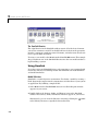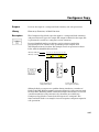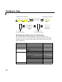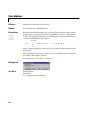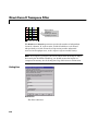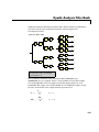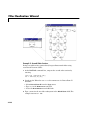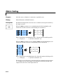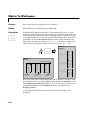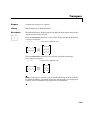
1
DSP Blockset For Use with SIMULINK S Modeling Simulation Implementation User’s Guide Version 3 How to Contact The MathWorks: ☎ ✉ 508-647-7000 Phone 508-647-7001 Fax The MathWorks, Inc. 24 Prime Park Way Natick, MA 01760-1500 Mail http://www.mathworks.com Web Anonymous FTP server Newsgroup ftp.mathworks.com comp.soft-sys.matlab @ [email protected] [email protected] [email protected] [email protected] [email protected] [email protected] [email protected] Technical support Product enhancement suggestions Bug reports Documentation error reports Subscribing user registration Order status, license renewals, passcodes Sales, pricing, and general information DSP Blockset User’s Guide COPYRIGHT 1995 - 1999 by The MathWorks, Inc. The software described in this document is furnished under a license agreement. The software may be used or copied only under the terms of the license agreement. No part of this manual may be photocopied or reproduced in any form without prior written consent from The MathWorks, Inc. U.S. GOVERNMENT: If Licensee is acquiring the Programs on behalf of any unit or agency of the U.S. Government, the following shall apply: (a) For units of the Department of Defense: the Government shall have only the rights specified in the license under which the commercial computer software or commercial software documentation was obtained, as set forth in subparagraph (a) of the Rights in Commercial Computer Software or Commercial Software Documentation Clause at DFARS 227.7202-3, therefore the rights set forth herein shall apply; and (b) For any other unit or agency: NOTICE: Notwithstanding any other lease or license agreement that may pertain to, or accompany the delivery of, the computer software and accompanying documentation, the rights of the Government regarding its use, reproduction, and disclosure are as set forth in Clause 52.227-19 (c)(2) of the FAR. MATLAB, Simulink, Stateflow, Handle Graphics, and Real-Time Workshop are registered trademarks, and Target Language Compiler is a trademark of The MathWorks, Inc. Other product or brand names are trademarks or registered trademarks of their respective holders. Printing History: April 1995 May 1997 January 1998 January 1999 First printing Second printing Third printing Fourth printing DSP Blockset 1.0 DSP Blockset 2.0 DSP Blockset 2.2 (R10) DSP Blockset 3.0 (R11) Contents Introduction 1 Welcome to the DSP Blockset . . . . . . . . . . . . . . . . . . . . . . . . . . 1-2 What Is the DSP Blockset? . . . . . . . . . . . . . . . . . . . . . . . . . . . . . Key Features . . . . . . . . . . . . . . . . . . . . . . . . . . . . . . . . . . . . . . . . Frame-Based Operations . . . . . . . . . . . . . . . . . . . . . . . . . . . . Matrix Support . . . . . . . . . . . . . . . . . . . . . . . . . . . . . . . . . . . . Adaptive and Multirate Filtering . . . . . . . . . . . . . . . . . . . . . . Statistical Operations . . . . . . . . . . . . . . . . . . . . . . . . . . . . . . . Linear Algebra . . . . . . . . . . . . . . . . . . . . . . . . . . . . . . . . . . . . . Parametric Estimation . . . . . . . . . . . . . . . . . . . . . . . . . . . . . . Real-Time Code Generation . . . . . . . . . . . . . . . . . . . . . . . . . . About the DSP Blockset Libraries . . . . . . . . . . . . . . . . . . . . . . . 1-3 1-3 1-3 1-4 1-4 1-5 1-5 1-5 1-5 1-5 What Is in the DSP Blockset? . . . . . . . . . . . . . . . . . . . . . . . . . . 1-7 DSP Sources Library . . . . . . . . . . . . . . . . . . . . . . . . . . . . . . . . . . 1-8 DSP Sinks Library . . . . . . . . . . . . . . . . . . . . . . . . . . . . . . . . . . . . 1-8 Math Functions Library . . . . . . . . . . . . . . . . . . . . . . . . . . . . . . . 1-8 Elementary Functions Library . . . . . . . . . . . . . . . . . . . . . . . . 1-9 Vector Functions Library . . . . . . . . . . . . . . . . . . . . . . . . . . . . 1-9 Matrix Functions Library . . . . . . . . . . . . . . . . . . . . . . . . . . . . 1-9 Linear Algebra Library . . . . . . . . . . . . . . . . . . . . . . . . . . . . . 1-10 Statistics Library . . . . . . . . . . . . . . . . . . . . . . . . . . . . . . . . . 1-10 General DSP Library . . . . . . . . . . . . . . . . . . . . . . . . . . . . . . . . . 1-11 Signal Operations Library . . . . . . . . . . . . . . . . . . . . . . . . . . 1-11 Transforms Library . . . . . . . . . . . . . . . . . . . . . . . . . . . . . . . . 1-11 Buffers Library . . . . . . . . . . . . . . . . . . . . . . . . . . . . . . . . . . . 1-12 Switches and Counters Library . . . . . . . . . . . . . . . . . . . . . . 1-12 Estimation Library . . . . . . . . . . . . . . . . . . . . . . . . . . . . . . . . . . 1-12 Parametric Estimation Library . . . . . . . . . . . . . . . . . . . . . . 1-13 Power Spectrum Estimation Library . . . . . . . . . . . . . . . . . . 1-13 i Filtering Library . . . . . . . . . . . . . . . . . . . . . . . . . . . . . . . . . . . . Filter Designs Library . . . . . . . . . . . . . . . . . . . . . . . . . . . . . . Filter Realizations Library . . . . . . . . . . . . . . . . . . . . . . . . . . Adaptive Filters Library . . . . . . . . . . . . . . . . . . . . . . . . . . . . Multirate Filters Library . . . . . . . . . . . . . . . . . . . . . . . . . . . Demos Library . . . . . . . . . . . . . . . . . . . . . . . . . . . . . . . . . . . . . . Installation . . . . . . . . . . . . . . . . . . . . . . . . . . . . . . . . . . . . . . . . . 1-13 1-13 1-14 1-14 1-15 1-15 1-15 Getting Started with the DSP Blockset . . . . . . . . . . . . . . . . . How to Get Help Online . . . . . . . . . . . . . . . . . . . . . . . . . . . . . . . How to Use This Guide . . . . . . . . . . . . . . . . . . . . . . . . . . . . . . . Technical Conventions . . . . . . . . . . . . . . . . . . . . . . . . . . . . . . Typographical Conventions . . . . . . . . . . . . . . . . . . . . . . . . . . Related Products and Documentation . . . . . . . . . . . . . . . . . . . What Is MATLAB? . . . . . . . . . . . . . . . . . . . . . . . . . . . . . . . . What Is Simulink? . . . . . . . . . . . . . . . . . . . . . . . . . . . . . . . . . What Is the Signal Processing Toolbox? . . . . . . . . . . . . . . . . What Is the Real-Time Workshop? . . . . . . . . . . . . . . . . . . . . 1-16 1-16 1-17 1-17 1-19 1-20 1-20 1-21 1-21 1-22 Simulink and the DSP Blockset 2 Overview . . . . . . . . . . . . . . . . . . . . . . . . . . . . . . . . . . . . . . . . . . . . . 2-2 Introduction to the Simulink Environment . . . . . . . . . . . . . . Starting Simulink . . . . . . . . . . . . . . . . . . . . . . . . . . . . . . . . . . . . Simulink on PC Platforms . . . . . . . . . . . . . . . . . . . . . . . . . . . . Simulink on UNIX Platforms . . . . . . . . . . . . . . . . . . . . . . . . . The Simulink Libraries . . . . . . . . . . . . . . . . . . . . . . . . . . . . . . Using Simulink . . . . . . . . . . . . . . . . . . . . . . . . . . . . . . . . . . . . . . Model Definition . . . . . . . . . . . . . . . . . . . . . . . . . . . . . . . . . . . Model Simulation . . . . . . . . . . . . . . . . . . . . . . . . . . . . . . . . . . . Learning More About Simulink . . . . . . . . . . . . . . . . . . . . . . . . . 2-3 2-3 2-3 2-3 2-4 2-4 2-4 2-6 2-7 Configuring Simulink for DSP Systems . . . . . . . . . . . . . . . . . 2-8 Using dspstartup.m . . . . . . . . . . . . . . . . . . . . . . . . . . . . . . . . . . . 2-8 Performance-Related Settings . . . . . . . . . . . . . . . . . . . . . . . . . . . 2-9 ii Contents Miscellaneous Settings . . . . . . . . . . . . . . . . . . . . . . . . . . . . . . . 2-12 Customizing dspstartup.m . . . . . . . . . . . . . . . . . . . . . . . . . . . . 2-12 Understanding Sample Rates . . . . . . . . . . . . . . . . . . . . . . . . . Discrete-Time Signals . . . . . . . . . . . . . . . . . . . . . . . . . . . . . . . . Time and Frequency Terminology . . . . . . . . . . . . . . . . . . . . Discrete-Time Signals in Simulink . . . . . . . . . . . . . . . . . . . . Inspecting Sample Rates . . . . . . . . . . . . . . . . . . . . . . . . . . . . . . Probe Block . . . . . . . . . . . . . . . . . . . . . . . . . . . . . . . . . . . . . . Sample Time Color Coding . . . . . . . . . . . . . . . . . . . . . . . . . . Types of Sampling . . . . . . . . . . . . . . . . . . . . . . . . . . . . . . . . . . . Source Blocks . . . . . . . . . . . . . . . . . . . . . . . . . . . . . . . . . . . . . Nonsource Blocks . . . . . . . . . . . . . . . . . . . . . . . . . . . . . . . . . . Rate Conversion . . . . . . . . . . . . . . . . . . . . . . . . . . . . . . . . . . . . . Direct Rate Conversion . . . . . . . . . . . . . . . . . . . . . . . . . . . . . Frame Rebuffering . . . . . . . . . . . . . . . . . . . . . . . . . . . . . . . . . Avoiding Unintended Rate Conversions . . . . . . . . . . . . . . . . 2-13 2-13 2-14 2-15 2-18 2-19 2-21 2-21 2-22 2-23 2-23 2-24 2-27 2-32 Understanding Matrices . . . . . . . . . . . . . . . . . . . . . . . . . . . . . . Sample-Based Matrices . . . . . . . . . . . . . . . . . . . . . . . . . . . . . . . Frame-Based Matrices . . . . . . . . . . . . . . . . . . . . . . . . . . . . . . . . Matrices and Signal-Oriented Blocks . . . . . . . . . . . . . . . . . . . . Matrices and Other Blocks . . . . . . . . . . . . . . . . . . . . . . . . . . . . Specifying Matrix Dimensions . . . . . . . . . . . . . . . . . . . . . . . . . Tracking Matrix Sizes . . . . . . . . . . . . . . . . . . . . . . . . . . . . . . Scalars and Vectors . . . . . . . . . . . . . . . . . . . . . . . . . . . . . . . . Using Matrices with Nonmatrix Blocks . . . . . . . . . . . . . . . . . . Passing Matrices to Element-Oriented Blocks . . . . . . . . . . Passing Matrices to Vector-Oriented Blocks . . . . . . . . . . . . Passing Matrices to Scalar-Oriented Blocks . . . . . . . . . . . . Matrix Input and Output . . . . . . . . . . . . . . . . . . . . . . . . . . . . . . 2-35 2-36 2-37 2-38 2-39 2-39 2-40 2-41 2-41 2-41 2-41 2-41 2-42 Understanding Samples and Frames . . . . . . . . . . . . . . . . . . . Sample Vectors and Sample Matrices . . . . . . . . . . . . . . . . . . . Working with Sample Vectors . . . . . . . . . . . . . . . . . . . . . . . . Working with Sample Matrices . . . . . . . . . . . . . . . . . . . . . . Frames and Frame Matrices . . . . . . . . . . . . . . . . . . . . . . . . . . . Working with Frame Vectors (Single-Channel Signals) . . . Working with Frame Matrices (Multichannel Signals) . . . . 2-43 2-44 2-44 2-47 2-50 2-50 2-53 iii Understanding Multichannel Signal Processing . . . . . . . . . . . Example 1: Sample-Based Operation with Vector Input . . Example 2: Sample-Based Operation with Vector Input . . Example 3: Frame-Based Operation with Vector Input . . . Example 4: Frame-Based Operation with Matrix Input . . . Benefits of Frame-Based Processing . . . . . . . . . . . . . . . . . . . . . Accelerating Real-Time Systems . . . . . . . . . . . . . . . . . . . . . Accelerating Simulations . . . . . . . . . . . . . . . . . . . . . . . . . . . 2-59 2-60 2-62 2-65 2-66 2-69 2-69 2-70 Increasing Performance . . . . . . . . . . . . . . . . . . . . . . . . . . . . . . 2-71 Using the DSP Blockset 3 Overview . . . . . . . . . . . . . . . . . . . . . . . . . . . . . . . . . . . . . . . . . . . . . 3-2 Working with Filter Designs . . . . . . . . . . . . . . . . . . . . . . . . . . . 3-3 Filter Designs Blocks . . . . . . . . . . . . . . . . . . . . . . . . . . . . . . . . . . 3-3 Frame-Based Processing . . . . . . . . . . . . . . . . . . . . . . . . . . . . . 3-4 Classical IIR and FIR Filters, Discrete Time . . . . . . . . . . . . . . . 3-5 Example: Chebyshev Type II Lowpass Filter . . . . . . . . . . . . 3-6 Classical IIR Filters, Continuous Time . . . . . . . . . . . . . . . . . . . 3-8 Special IIR and FIR Filters, Discrete-Time . . . . . . . . . . . . . . . 3-10 Filter Design Characteristics . . . . . . . . . . . . . . . . . . . . . . . . 3-10 Frequency and Magnitude Parameters . . . . . . . . . . . . . . . . 3-11 Weight Parameters . . . . . . . . . . . . . . . . . . . . . . . . . . . . . . . . 3-13 Example: Least Squares Multiband Filter . . . . . . . . . . . . . . 3-14 Working with Windows . . . . . . . . . . . . . . . . . . . . . . . . . . . . . . . Generating a Window . . . . . . . . . . . . . . . . . . . . . . . . . . . . . . . . Applying a Window . . . . . . . . . . . . . . . . . . . . . . . . . . . . . . . . . . Generating and Applying a Window . . . . . . . . . . . . . . . . . . . . . Window Specifications . . . . . . . . . . . . . . . . . . . . . . . . . . . . . . . . 3-17 3-18 3-18 3-18 3-19 Working with Buffers . . . . . . . . . . . . . . . . . . . . . . . . . . . . . . . . . 3-20 Buffering Sample-Based Signals . . . . . . . . . . . . . . . . . . . . . . . . 3-22 iv Contents Rebuffering Frame-Based Signals . . . . . . . . . . . . . . . . . . . . . . Example: Single-Channel Rebuffering . . . . . . . . . . . . . . . . . Example: Multichannel Rebuffering . . . . . . . . . . . . . . . . . . . Unbuffering Frame-Based Signals . . . . . . . . . . . . . . . . . . . . . . The Unbuffer Block . . . . . . . . . . . . . . . . . . . . . . . . . . . . . . . . The Partial Unbuffer Block . . . . . . . . . . . . . . . . . . . . . . . . . . Using Overlapping Buffers . . . . . . . . . . . . . . . . . . . . . . . . . . . . Initial State of Buffer Blocks . . . . . . . . . . . . . . . . . . . . . . . . . . . The Buffer and Rebuffer Blocks . . . . . . . . . . . . . . . . . . . . . . The Unbuffer and Partial Unbuffer Blocks . . . . . . . . . . . . . Example: Using Buffer and Unbuffer . . . . . . . . . . . . . . . . . . . . Example: Convolution . . . . . . . . . . . . . . . . . . . . . . . . . . . . . . . . 3-24 3-26 3-26 3-27 3-27 3-28 3-29 3-30 3-30 3-31 3-33 3-35 Working with Sources and Sinks . . . . . . . . . . . . . . . . . . . . . . Importing Data from the Workspace . . . . . . . . . . . . . . . . . . . . Signal From Workspace . . . . . . . . . . . . . . . . . . . . . . . . . . . . Triggered Signal From Workspace . . . . . . . . . . . . . . . . . . . . Matrix From Workspace . . . . . . . . . . . . . . . . . . . . . . . . . . . . Exporting Data to the Workspace . . . . . . . . . . . . . . . . . . . . . . . Signal To Workspace . . . . . . . . . . . . . . . . . . . . . . . . . . . . . . . Matrix To Workspace . . . . . . . . . . . . . . . . . . . . . . . . . . . . . . Viewing Data with Scopes . . . . . . . . . . . . . . . . . . . . . . . . . . . . . 3-37 3-37 3-38 3-40 3-40 3-41 3-41 3-42 3-43 Working with Statistical Operations . . . . . . . . . . . . . . . . . . . Basic Operations . . . . . . . . . . . . . . . . . . . . . . . . . . . . . . . . . . . . Running Operations . . . . . . . . . . . . . . . . . . . . . . . . . . . . . . . . . . Demonstration Model: Running Operation . . . . . . . . . . . . . Example: Sliding Windows . . . . . . . . . . . . . . . . . . . . . . . . . . 3-45 3-46 3-47 3-48 3-49 DSP Blockset Demos . . . . . . . . . . . . . . . . . . . . . . . . . . . . . . . . . 3-51 DSP Block Reference 4 Using the DSP Block Reference Chapter . . . . . . . . . . . . . . . . 4-2 What Each Block Reference Page Contains . . . . . . . . . . . . . . . . 4-2 About Tunable Parameters . . . . . . . . . . . . . . . . . . . . . . . . . . . 4-2 v Block Library Hierarchy . . . . . . . . . . . . . . . . . . . . . . . . . . . . . . . 4-3 Block Library Contents . . . . . . . . . . . . . . . . . . . . . . . . . . . . . . . . 4-3 Analog Filter Design . . . . . . . . . . . . . . . . . . . . . . . . . . . . . . . . 4-9 Analytic Signal . . . . . . . . . . . . . . . . . . . . . . . . . . . . . . . . . . . . 4-13 Autocorrelation . . . . . . . . . . . . . . . . . . . . . . . . . . . . . . . . . . . 4-15 Backward Substitution . . . . . . . . . . . . . . . . . . . . . . . . . . . . . 4-17 Biquadratic Filter . . . . . . . . . . . . . . . . . . . . . . . . . . . . . . . . . 4-18 Buffer . . . . . . . . . . . . . . . . . . . . . . . . . . . . . . . . . . . . . . . . . . . 4-21 Buffered FFT Frame Scope . . . . . . . . . . . . . . . . . . . . . . . . . . 4-25 Burg AR Estimator . . . . . . . . . . . . . . . . . . . . . . . . . . . . . . . . 4-29 Burg Method . . . . . . . . . . . . . . . . . . . . . . . . . . . . . . . . . . . . . 4-31 Chirp . . . . . . . . . . . . . . . . . . . . . . . . . . . . . . . . . . . . . . . . . . . . 4-34 Cholesky Factorization . . . . . . . . . . . . . . . . . . . . . . . . . . . . . 4-37 Cholesky Solver . . . . . . . . . . . . . . . . . . . . . . . . . . . . . . . . . . . 4-39 Commutator . . . . . . . . . . . . . . . . . . . . . . . . . . . . . . . . . . . . . . 4-41 Complex Cepstrum . . . . . . . . . . . . . . . . . . . . . . . . . . . . . . . . 4-42 Complex Exponential . . . . . . . . . . . . . . . . . . . . . . . . . . . . . . . 4-43 Constant Diagonal Matrix . . . . . . . . . . . . . . . . . . . . . . . . . . . 4-44 Contiguous Copy . . . . . . . . . . . . . . . . . . . . . . . . . . . . . . . . . . 4-45 Convert Complex DSP To Simulink . . . . . . . . . . . . . . . . . . . 4-49 Convert Complex Simulink To DSP . . . . . . . . . . . . . . . . . . . 4-51 Convolution . . . . . . . . . . . . . . . . . . . . . . . . . . . . . . . . . . . . . . 4-53 Correlation . . . . . . . . . . . . . . . . . . . . . . . . . . . . . . . . . . . . . . . 4-54 Counter . . . . . . . . . . . . . . . . . . . . . . . . . . . . . . . . . . . . . . . . . . 4-55 Covariance AR Estimator . . . . . . . . . . . . . . . . . . . . . . . . . . . 4-60 Covariance Method . . . . . . . . . . . . . . . . . . . . . . . . . . . . . . . . 4-62 Create Diagonal Matrix . . . . . . . . . . . . . . . . . . . . . . . . . . . . . 4-64 Cumulative Sum . . . . . . . . . . . . . . . . . . . . . . . . . . . . . . . . . . 4-65 dB . . . . . . . . . . . . . . . . . . . . . . . . . . . . . . . . . . . . . . . . . . . . . . 4-66 dB Gain . . . . . . . . . . . . . . . . . . . . . . . . . . . . . . . . . . . . . . . . . 4-67 DCT . . . . . . . . . . . . . . . . . . . . . . . . . . . . . . . . . . . . . . . . . . . . 4-68 Detrend . . . . . . . . . . . . . . . . . . . . . . . . . . . . . . . . . . . . . . . . . . 4-70 Difference . . . . . . . . . . . . . . . . . . . . . . . . . . . . . . . . . . . . . . . . 4-71 Digital FIR Filter Design . . . . . . . . . . . . . . . . . . . . . . . . . . . 4-72 Digital IIR Filter Design . . . . . . . . . . . . . . . . . . . . . . . . . . . . 4-79 Direct-Form II Transpose Filter . . . . . . . . . . . . . . . . . . . . . . 4-84 Discrete Constant . . . . . . . . . . . . . . . . . . . . . . . . . . . . . . . . . 4-88 Distributor . . . . . . . . . . . . . . . . . . . . . . . . . . . . . . . . . . . . . . . 4-89 Downsample . . . . . . . . . . . . . . . . . . . . . . . . . . . . . . . . . . . . . . 4-91 Dyadic Analysis Filter Bank . . . . . . . . . . . . . . . . . . . . . . . . . 4-96 vi Contents Dyadic Synthesis Filter Bank . . . . . . . . . . . . . . . . . . . . . . . Edge Detector . . . . . . . . . . . . . . . . . . . . . . . . . . . . . . . . . . . . Event-Count Comparator . . . . . . . . . . . . . . . . . . . . . . . . . . Extract Diagonal . . . . . . . . . . . . . . . . . . . . . . . . . . . . . . . . . Extract Triangular Matrix . . . . . . . . . . . . . . . . . . . . . . . . . FFT . . . . . . . . . . . . . . . . . . . . . . . . . . . . . . . . . . . . . . . . . . . . FFT Frame Scope . . . . . . . . . . . . . . . . . . . . . . . . . . . . . . . . . Filter Realization Wizard . . . . . . . . . . . . . . . . . . . . . . . . . . FIR Decimation . . . . . . . . . . . . . . . . . . . . . . . . . . . . . . . . . . FIR Interpolation . . . . . . . . . . . . . . . . . . . . . . . . . . . . . . . . . FIR Rate Conversion . . . . . . . . . . . . . . . . . . . . . . . . . . . . . . Flip . . . . . . . . . . . . . . . . . . . . . . . . . . . . . . . . . . . . . . . . . . . . Forward Substitution . . . . . . . . . . . . . . . . . . . . . . . . . . . . . Frequency Frame Scope . . . . . . . . . . . . . . . . . . . . . . . . . . . From Wave Device . . . . . . . . . . . . . . . . . . . . . . . . . . . . . . . . From Wave File . . . . . . . . . . . . . . . . . . . . . . . . . . . . . . . . . . Histogram . . . . . . . . . . . . . . . . . . . . . . . . . . . . . . . . . . . . . . . IDCT . . . . . . . . . . . . . . . . . . . . . . . . . . . . . . . . . . . . . . . . . . . IFFT . . . . . . . . . . . . . . . . . . . . . . . . . . . . . . . . . . . . . . . . . . . Inherit Complexity . . . . . . . . . . . . . . . . . . . . . . . . . . . . . . . . Integer Delay . . . . . . . . . . . . . . . . . . . . . . . . . . . . . . . . . . . . Kalman Adaptive Filter . . . . . . . . . . . . . . . . . . . . . . . . . . . . LDL Factorization . . . . . . . . . . . . . . . . . . . . . . . . . . . . . . . . LDL Solver . . . . . . . . . . . . . . . . . . . . . . . . . . . . . . . . . . . . . . Least Squares FIR Filter Design . . . . . . . . . . . . . . . . . . . . Levinson Solver . . . . . . . . . . . . . . . . . . . . . . . . . . . . . . . . . . LMS Adaptive Filter . . . . . . . . . . . . . . . . . . . . . . . . . . . . . . LPC . . . . . . . . . . . . . . . . . . . . . . . . . . . . . . . . . . . . . . . . . . . . LU Factorization . . . . . . . . . . . . . . . . . . . . . . . . . . . . . . . . . LU Solver . . . . . . . . . . . . . . . . . . . . . . . . . . . . . . . . . . . . . . . Magnitude FFT . . . . . . . . . . . . . . . . . . . . . . . . . . . . . . . . . . Matrix 1-Norm . . . . . . . . . . . . . . . . . . . . . . . . . . . . . . . . . . . Matrix Constant . . . . . . . . . . . . . . . . . . . . . . . . . . . . . . . . . . Matrix From Workspace . . . . . . . . . . . . . . . . . . . . . . . . . . . Matrix Multiplication . . . . . . . . . . . . . . . . . . . . . . . . . . . . . Matrix Product . . . . . . . . . . . . . . . . . . . . . . . . . . . . . . . . . . . Matrix Scaling . . . . . . . . . . . . . . . . . . . . . . . . . . . . . . . . . . . Matrix Sum . . . . . . . . . . . . . . . . . . . . . . . . . . . . . . . . . . . . . Matrix To Workspace . . . . . . . . . . . . . . . . . . . . . . . . . . . . . Matrix Viewer . . . . . . . . . . . . . . . . . . . . . . . . . . . . . . . . . . . 4-103 4-110 4-112 4-114 4-115 4-117 4-119 4-123 4-133 4-137 4-141 4-145 4-146 4-147 4-151 4-156 4-158 4-163 4-164 4-166 4-168 4-177 4-182 4-184 4-186 4-191 4-194 4-197 4-200 4-202 4-204 4-206 4-208 4-209 4-211 4-212 4-214 4-216 4-218 4-220 vii Maximum . . . . . . . . . . . . . . . . . . . . . . . . . . . . . . . . . . . . . . . Mean . . . . . . . . . . . . . . . . . . . . . . . . . . . . . . . . . . . . . . . . . . . Median . . . . . . . . . . . . . . . . . . . . . . . . . . . . . . . . . . . . . . . . . Minimum . . . . . . . . . . . . . . . . . . . . . . . . . . . . . . . . . . . . . . . Modified Covariance AR Estimator . . . . . . . . . . . . . . . . . . Modified Covariance Method . . . . . . . . . . . . . . . . . . . . . . . Multiphase Clock . . . . . . . . . . . . . . . . . . . . . . . . . . . . . . . . . N-Sample Enable . . . . . . . . . . . . . . . . . . . . . . . . . . . . . . . . . N-Sample Switch . . . . . . . . . . . . . . . . . . . . . . . . . . . . . . . . . Normalization . . . . . . . . . . . . . . . . . . . . . . . . . . . . . . . . . . . Overlap-Add FFT Filter . . . . . . . . . . . . . . . . . . . . . . . . . . . Overlap-Save FFT Filter . . . . . . . . . . . . . . . . . . . . . . . . . . . Partial Unbuffer . . . . . . . . . . . . . . . . . . . . . . . . . . . . . . . . . . Permute Matrix . . . . . . . . . . . . . . . . . . . . . . . . . . . . . . . . . . QR Factorization . . . . . . . . . . . . . . . . . . . . . . . . . . . . . . . . . QR Solver . . . . . . . . . . . . . . . . . . . . . . . . . . . . . . . . . . . . . . . Queue . . . . . . . . . . . . . . . . . . . . . . . . . . . . . . . . . . . . . . . . . . Real Cepstrum . . . . . . . . . . . . . . . . . . . . . . . . . . . . . . . . . . . Rebuffer . . . . . . . . . . . . . . . . . . . . . . . . . . . . . . . . . . . . . . . . Reciprocal Condition . . . . . . . . . . . . . . . . . . . . . . . . . . . . . . Remez FIR Filter Design . . . . . . . . . . . . . . . . . . . . . . . . . . . Repeat . . . . . . . . . . . . . . . . . . . . . . . . . . . . . . . . . . . . . . . . . . Reshape . . . . . . . . . . . . . . . . . . . . . . . . . . . . . . . . . . . . . . . . RLS Adaptive Filter . . . . . . . . . . . . . . . . . . . . . . . . . . . . . . . RMS . . . . . . . . . . . . . . . . . . . . . . . . . . . . . . . . . . . . . . . . . . . Sample and Hold . . . . . . . . . . . . . . . . . . . . . . . . . . . . . . . . . Shift Register . . . . . . . . . . . . . . . . . . . . . . . . . . . . . . . . . . . . Short-Time FFT . . . . . . . . . . . . . . . . . . . . . . . . . . . . . . . . . . Signal From Workspace . . . . . . . . . . . . . . . . . . . . . . . . . . . Signal To Workspace . . . . . . . . . . . . . . . . . . . . . . . . . . . . . . Sine Wave . . . . . . . . . . . . . . . . . . . . . . . . . . . . . . . . . . . . . . . Discrete Computational Methods . . . . . . . . . . . . . . . . . . . . Sort . . . . . . . . . . . . . . . . . . . . . . . . . . . . . . . . . . . . . . . . . . . . Stack . . . . . . . . . . . . . . . . . . . . . . . . . . . . . . . . . . . . . . . . . . . Standard Deviation . . . . . . . . . . . . . . . . . . . . . . . . . . . . . . . Submatrix . . . . . . . . . . . . . . . . . . . . . . . . . . . . . . . . . . . . . . . Time Frame Scope . . . . . . . . . . . . . . . . . . . . . . . . . . . . . . . . Time-Varying Direct-Form II Transpose Filter . . . . . . . . . Time-Varying Lattice Filter . . . . . . . . . . . . . . . . . . . . . . . . Toeplitz . . . . . . . . . . . . . . . . . . . . . . . . . . . . . . . . . . . . . . . . . viii Contents 4-226 4-230 4-234 4-235 4-239 4-241 4-243 4-246 4-248 4-250 4-252 4-254 4-256 4-261 4-264 4-266 4-268 4-273 4-274 4-282 4-284 4-289 4-293 4-294 4-297 4-301 4-303 4-306 4-309 4-311 4-314 4-315 4-320 4-322 4-327 4-331 4-333 4-345 4-350 4-354 To Wave Device . . . . . . . . . . . . . . . . . . . . . . . . . . . . . . . . . . To Wave File . . . . . . . . . . . . . . . . . . . . . . . . . . . . . . . . . . . . Transpose . . . . . . . . . . . . . . . . . . . . . . . . . . . . . . . . . . . . . . . Triggered Matrix To Workspace . . . . . . . . . . . . . . . . . . . . . Triggered Shift Register . . . . . . . . . . . . . . . . . . . . . . . . . . . Triggered Signal From Workspace . . . . . . . . . . . . . . . . . . . Triggered Signal To Workspace . . . . . . . . . . . . . . . . . . . . . Unbuffer . . . . . . . . . . . . . . . . . . . . . . . . . . . . . . . . . . . . . . . . Unwrap . . . . . . . . . . . . . . . . . . . . . . . . . . . . . . . . . . . . . . . . . Upsample . . . . . . . . . . . . . . . . . . . . . . . . . . . . . . . . . . . . . . . User-Defined Frame Scope . . . . . . . . . . . . . . . . . . . . . . . . . Variable Fractional Delay . . . . . . . . . . . . . . . . . . . . . . . . . . Variable Integer Delay . . . . . . . . . . . . . . . . . . . . . . . . . . . . Variable Selector . . . . . . . . . . . . . . . . . . . . . . . . . . . . . . . . . Variance . . . . . . . . . . . . . . . . . . . . . . . . . . . . . . . . . . . . . . . . Window Function . . . . . . . . . . . . . . . . . . . . . . . . . . . . . . . . . Yule-Walker AR Estimator . . . . . . . . . . . . . . . . . . . . . . . . . Yule-Walker IIR Filter Design . . . . . . . . . . . . . . . . . . . . . . Yule-Walker Method . . . . . . . . . . . . . . . . . . . . . . . . . . . . . . Zero Pad . . . . . . . . . . . . . . . . . . . . . . . . . . . . . . . . . . . . . . . . 4-356 4-361 4-363 4-365 4-368 4-372 4-375 4-377 4-380 4-381 4-385 4-390 4-396 4-406 4-408 4-412 4-416 4-418 4-421 4-423 DSP Function Reference 5 DSP Blockset Utility Functions . . . . . . . . . . . . . . . . . . . . . . . . . dsp_links . . . . . . . . . . . . . . . . . . . . . . . . . . . . . . . . . . . . . . . . . dsplib . . . . . . . . . . . . . . . . . . . . . . . . . . . . . . . . . . . . . . . . . . . . dspstartup . . . . . . . . . . . . . . . . . . . . . . . . . . . . . . . . . . . . . . . . liblinks . . . . . . . . . . . . . . . . . . . . . . . . . . . . . . . . . . . . . . . . . . rebuffer_delay . . . . . . . . . . . . . . . . . . . . . . . . . . . . . . . . . . . . 5-2 5-3 5-4 5-5 5-7 5-8 ix x Contents 1 Introduction Welcome to the DSP Blockset . . . . . . . . . . . . 1-2 What Is the DSP Blockset? . . . . . . . . . . . . . 1-3 Key Features . . . . . . . . . . . . . . . . . . . . 1-3 About the DSP Blockset Libraries . . . . . . . . . . . . 1-5 What Is in the DSP Blockset? DSP Sources Library . . . . . DSP Sinks Library . . . . . . Math Functions Library . . . . General DSP Library . . . . . Estimation Library . . . . . . Filtering Library . . . . . . . Demos Library . . . . . . . . Installation . . . . . . . . . . . . . . . . . . . . . . . . . . . . . . . . . . . . . . . . . . . . . . . . . . . . . . . . . . . . . . . . . . . . . . . . . . . . . . . . . . . . . . . . . . . . . . . . . . . . . . . . . . . . . . . . . . . . . 1-7 1-8 1-8 1-8 1-11 1-12 1-13 1-15 1-15 Getting Started with the DSP Blockset How to Get Help Online . . . . . . . . How to Use This Guide . . . . . . . . Related Products and Documentation . . . . . . . . . . . . . . . . . . . . . . . . . . . . . . . . . . 1-16 1-16 1-17 1-20 1 Introduction Welcome to the DSP Blockset Welcome to the DSP Blockset, the premier tool for digital signal processing (DSP) algorithm simulation and code generation. The DSP Blockset brings the full power of Simulink® to DSP system design and prototyping by providing key DSP algorithms and components in Simulink’s adaptable block format. From buffers to linear algebra solvers, from dyadic filter banks to parametric estimators, the blockset gives you all the core components to rapidly and efficiently assemble complex DSP systems. Use the DSP Blockset and Simulink to develop your DSP concepts, and to efficiently revise and test until the design is production-ready. Use the DSP Blockset together with the Real-Time Workshop® (RTW) to automatically generate code for real-time execution on DSP hardware. Above all, we hope you enjoy using the DSP Blockset, and we look forward to hearing your comments and suggestions. [email protected] [email protected] [email protected] [email protected] Technical support Product enhancement suggestions Bug reports Documentation error reports Visit the MathWorks Web site at www.mathworks.com for complete contact information. 1-2 What Is the DSP Blockset? What Is the DSP Blockset? The DSP Blockset is a collection of block libraries for use with the Simulink dynamic system simulation environment. The DSP Blockset libraries are designed specifically for digital signal processing (DSP) applications, and include key operations such as classical, multirate, and adaptive filtering, matrix manipulation and linear algebra, statistics, time-frequency transforms, and more. Key Features The DSP Blockset extends the Simulink environment by providing core components and algorithms for DSP systems. You can use blocks from the DSP Blockset in the same way that you would use any other Simulink blocks, combining them with blocks from other libraries to create sophisticated DSP systems. A few of the important features are: • Frame-based operations • Matrix support • Adaptive and multirate filtering • Statistical operations • Linear algebra • Parametric estimation • Real-time code generation capability Frame-Based Operations Most real-time DSP systems optimize throughput rates by processing data in “batch” or “frame-based” mode, where each batch or frame is a collection of consecutive signal samples that have been buffered into a single unit. By propagating these multisample frames instead of the individual signal samples, the DSP system can best take advantage of the speed of DSP algorithm execution, while simultaneously reducing the demands placed on the data acquisition (DAQ) hardware. The DSP Blockset delivers this same high level of performance for both simulation and code generation by incorporating frame-processing capability 1-3 1 Introduction into all of its blocks. A completely frame-based model can run several times faster than the same model processing sample-by-sample; even faster if the data source is frame based. See “Understanding Sample Rates” and “Understanding Samples and Frames” in Chapter 2 for complete information. Matrix Support The DSP Blockset supports two-dimensional matrices. Typical uses of the matrix format are: • General A matrix can be used in its traditional mathematical capacity, as a simple structured array of numbers. The matrix values might represent the pixel brightnesses from a charge-coupled device (CCD) camera, a collection of measurements from several tests, or any other group of values. Most blocks for general matrix operations are found in the Matrix Functions and Linear Algebra libraries. • To store factored submatrices A number of the matrix factorization blocks in the Linear Algebra library store the submatrix factors (i.e., lower and upper submatrices) in a single compound matrix. • To represent multichannel frame-based data The standard format for multichannel frame-based data is a matrix containing each channel’s data in a separate column. A matrix with three columns, for example, contains three channels of data, one frame per channel. The number of rows in such a matrix is the number of samples in each frame. See “Understanding Matrices” in Chapter 2 for complete information. Adaptive and Multirate Filtering The Adaptive Filters and Multirate Filters libraries provide key tools for the construction of advanced DSP systems. Adaptive filter blocks are parameterized to support the rapid tailoring of DSP algorithms to application-specific environments, and effortless “what if” experimentation. The multirate filtering algorithms employ polyphase implementations for efficient simulation and real-time code execution. 1-4 What Is the DSP Blockset? Statistical Operations Use the blocks in the Statistics library for basic statistical analysis. These blocks calculate measures of central tendency and spread (e.g., mean, standard deviation, and so on), as well as the frequency distribution of input values (histogram). Linear Algebra The Linear Algebra library provides a wide variety of matrix factorization methods, and equation solvers based on these methods. The popular Cholesky, LU, LDL, and QR factorizations are all available. Parametric Estimation The Parametric Estimation library provides a number of methods for modeling a signal as the output of an AR system. The methods include the Burg AR Estimator, Covariance AR Estimator, Modified Covariance AR Estimator, and Yule-Walker AR Estimator, which allow you to compute the AR system parameters based on forward error minimization, backward error minimization, or both. Real-Time Code Generation You can also use the separate Real-Time Workshop product to generate optimized, compact, C code for models containing blocks from the DSP Blockset. About the DSP Blockset Libraries Library Terms. The blocks in the DSP Blockset are organized into several libraries, whose contents and structure are shown on the following pages. The Blockset hierarchy has two levels of libraries. At the top level, some libraries (such as DSP Sources) contain DSP blocks, while others (such as Filtering) contain a second level of DSP libraries. This book uses the term “library” to refer to libraries at both levels in the hierarchy. So, for example, the Filtering library contains the Filter Designs library. True Libraries. The libraries in the DSP Blockset are true libraries. This means that when a block is copied from a DSP Blockset library to the model window, a reference to the source block (in the library) is created. Any updates made to 1-5 1 Introduction the source block will affect every model block that refers to it. For complete information about true libraries, see Using Simulink. 1-6 What Is in the DSP Blockset? What Is in the DSP Blockset? The organization of the DSP Blockset is shown in the figure below. Type dsplib in the command window to open the blockset. Each of the libraries in the DSP Blockset contains a collection of related DSP blocks or a group of more specialized libraries. Double-click on any library to display its contents. 1-7 1 Introduction DSP Sources Library The DSP Sources library provides blocks for acquiring data from devices, files, and the workspace, and for generating signals. DSP Sources Chirp Matrix From Workspace Constant Diagonal Matrix N-Sample Enable Discrete Constant Signal From Workspace From Wave Device Triggered Signal From Workspace From Wave File Sine Wave Matrix Constant DSP Sinks Library The DSP Sinks library provides blocks for sending data to devices, files, and the workspace, and for displaying signals on the screen in the time or frequency domain. DSP Sinks Buffered FFT Frame Scope Time Frame Scope FFT Frame Scope To Wave Device Frequency Frame Scope To Wave File Matrix To Workspace Triggered Matrix To Workspace Matrix Viewer Triggered Signal To Workspace Signal To Workspace User-Defined Frame Scope Math Functions Library The Math Functions library contains five sublibraries covering a wide variety of mathematical operations. 1-8 What Is in the DSP Blockset? Elementary Functions Library The Elementary Functions library provides an assortment of general conversion and utility blocks. Elementary Functions Complex Exponential dB Contiguous Copy dB Gain Convert Complex DSP To Simulink Inherit Complexity Convert Complex Simulink To DSP Variable Selector Vector Functions Library The Vector Functions library provides blocks for vector operations such as correlation and convolution. Vector Functions Autocorrelation Difference Convolution Flip Correlation Normalization Cumulative Sum Unwrap Matrix Functions Library The Matrix Functions library provides a variety of matrix-oriented operations, such as transposition, permutation, matrix arithmetic, and scaling. Matrix Functions Constant Diagonal Matrix Matrix Scaling Create Diagonal Matrix Matrix Sum Extract Diagonal Matrix To Workspace Extract Triangular Matrix Permute Matrix Matrix 1-Norm Reshape Matrix Constant Submatrix Matrix From Workspace Toeplitz 1-9 1 Introduction Matrix Functions (Continued) Matrix Multiplication Transpose Matrix Product Linear Algebra Library The Linear Algebra library provides blocks for matrix factorization and linear equation solution. Linear Algebra Backward Substitution Levinson Solver Cholesky Factorization LU Factorization Cholesky Solver LU Solver Forward Substitution QR Factorization LDL Factorization QR Solver LDL Solver Reciprocal Condition Statistics Library The Statistics library provides blocks for sorting data, and for computing static and cumulative statistical measures of central tendency, spread, and frequency distribution. Statistics Histogram RMS Maximum Sort Mean Standard Deviation Median Variance Minimum 1-10 What Is in the DSP Blockset? General DSP Library The General DSP library contains four sublibraries covering a wide variety of signal processing operations. Signal Operations Library The Signal Operations library provides blocks for common signal processing operations such as windowing, resampling, zero padding, and delay. Signal Operations Analytic Signal Upsample Detrend Variable Fractional Delay Downsample Variable Integer Delay Integer Delay Window Function LPC Zero Pad Repeat Transforms Library The Transforms library provides blocks for FFT, DCT, and cepstrum operations. Transforms Complex Cepstrum IDCT DCT IFFT FFT Real Cepstrum 1-11 1 Introduction Buffers Library The Buffers library provides blocks for rebuffering signals to different frame sizes, and for FIFO/LIFO storage. Buffers Buffer Shift Register Partial Unbuffer Stack Queue Triggered Shift Register Rebuffer Unbuffer Switches and Counters Library The Switches and Counters library provides blocks for switching signal sources, and for detecting and counting signal transitions. Switches and Counters Commutator Multiphase Clock Counter N-Sample Enable Distributor N-Sample Switch Edge Detector Sample and Hold Event-Count Comparator Estimation Library The Estimation library contains two sublibraries providing blocks for parametric estimation and power spectrum estimation. 1-12 What Is in the DSP Blockset? Parametric Estimation Library The Parametric Estimation library provides blocks for estimating the parameters of the autoregressive system generating the input. Parametric Estimation Burg AR Estimator Modified Covariance AR Estimator Covariance AR Estimator Yule-Walker AR Estimator Power Spectrum Estimation Library The Power Spectrum Estimation library provides blocks for estimating the power spectrum of the input by several different methods. Power Spectrum Estimation Burg Method Modified Covariance Method Covariance Method Short-Time FFT Magnitude FFT Yule-Walker Method Filtering Library The Filtering library contains four sublibraries providing blocks for a wide range of filtering applications. Filter Designs Library The Filter Designs library provides blocks for a variety of analog and digital FIR and IIR filter designs. Included are Butterworth, Chebyshev, elliptic, 1-13 1 Introduction differentiator, and Hilbert designs, in lowpass, highpass, bandpass, bandstop, and multiband configurations. Filter Designs Analog Filter Design Least Squares FIR Filter Design Digital FIR Filter Design Remez FIR Filter Design Digital IIR Filter Design Yule-Walker IIR Filter Design Filter Realizations Library The Filter Realizations library provides blocks and a Filter Realization Wizard for implementing a number of standard filter architectures, including timeand frequency-domain structures. Filter Realizations Biquadratic Filter Overlap-Save FFT Filter Direct-Form II Transpose Filter Time-Varying Direct-Form II Transpose Filter Filter Realization Wizard Time-Varying Lattice Filter Overlap-Add FFT Filter Adaptive Filters Library The Adaptive Filters library provides blocks for the adaptive determination of unknown filter coefficients, which is important in a wide variety of DSP operations, such as equalization and prediction. Adaptive Filters Kalman Adaptive Filter LMS Adaptive Filter 1-14 RLS Adaptive Filter What Is in the DSP Blockset? Multirate Filters Library The Multirate Filters library provides blocks for the efficient implementation of rate-conversion algorithms, as well as dyadic synthesis and analysis. Multirate Filters Dyadic Analysis Filter Bank FIR Interpolation Dyadic Synthesis Filter Bank FIR Rate Conversion FIR Decimation Demos Library The Demos library calls up the MATLAB® Demos window with the DSP Blockset demos selected. Double-click on a demo in the list to open that model, and select Start from the Simulation menu to run it. Installation The DSP Blockset follows the same installation procedure as the MATLAB toolboxes. See the MATLAB Installation Guide for PC or the MATLAB Installation Guide for UNIX. 1-15 1 Introduction Getting Started with the DSP Blockset To open the DSP Blockset, type dsplib at the MATLAB command line or right-click the DSP Blockset listing in the Simulink Library Browser. Double-click on any library in the DSP Blockset to view its contents, and double-click on a block to access its parameter dialog box. How to Get Help Online There are a number of easy ways to get help on the DSP Blockset while you’re working at the computer. • Block Help: Press the Help button in any block dialog box to view the online reference documentation for that block. • Simulink Library Browser: Right-click on a block name to access the help for that block. • Help Desk: Select Help Desk from the MATLAB Help menu, or type helpdesk or doc at the command line, to access the Help Desk facility. • Release Information: Type info dspblks at the MATLAB command line to view information related to the version of the DSP Blockset that you’re using, and to find out about recent changes to the blockset. 1-16 Getting Started with the DSP Blockset How to Use This Guide This book contains tutorial sections that are designed to help you become familiar with using Simulink and the DSP Blockset, as well as a reference section for finding detailed information on particular blocks in the blockset. • Read Chapter 2 of this guide, “Simulink and the DSP Blockset,” to get an overview of fundamental Simulink and DSP Blockset concepts. Also see Using Simulink for more information on the Simulink environment. • Read Chapter 3 of this guide, “Using the DSP Blockset,” for details on key operations common to many signal processing tasks, and a discussion of block applications. • Read Chapter 4, “DSP Block Reference,” for a description of each block’s operation, parameters, and characteristics. • Read the “DSP Blockset” sections of Release 11 New Features and Known Software and Documentation Problems to learn about enhancements made to the blockset in the current version. Use this guide in conjunction with the software to learn about the powerful features that the DSP Blockset provides. Technical Conventions Vectors. In this book, and in the block dialog boxes, the terms width and length are used interchangeably to describe the size of a vector, buffer, or frame: u = [1 2 3 4 5] u = 1:25 u = [1:64]' % a vector of length N=5 % a buffer of width 25 % a length-64 frame When a vector represents a frame of data (frame vector), it is usually shown as a column vector with the most recent sample in the last position, u(end). When a vector represents data from multiple channels (sample vector), it is usually shown as a row vector with the first channel in the leftmost position, u(1). 1-17 Introduction Length-8 frame vector 1 2 3 4 5 6 7 8 sample 1 sample 2 sample 3 sample 4 sample 5 sample 6 sample 7 sample 8 Length-8 sample vector 1 23 456 78 channel 1 channel 2 channel 3 channel 4 channel 5 channel 6 channel 7 channel 8 1 See “Understanding Matrices” and “Understanding Samples and Frames” in Chapter 2 for more information about these different representations. Matrices. Matrix dimensions are described in terms of the number of rows and the number of columns of the matrix: u = [1 2 3;4 5 6] % a 2-by-3 matrix The number of channels in a frame-based matrix is the number of columns. Arrays. The number of pages of a three-dimensional array (in the MATLAB workspace) refers to the size of its third dimension: A(:,:,1) = [1 2 3;4 5 6] A(:,:,2) = [7 8 9;0 1 2] A(:,:,3) = [3 4 5;6 7 8] % the first page of a 3-page array % the second page % the last page Important sampling-related notational conventions are listed in “Understanding Sample Rates” in Chapter 2. 1-18 Getting Started with the DSP Blockset Typographical Conventions To Indicate This Manual Uses Example Example code Monospace type To assign the value 5 to A, enter A = 5 MATLAB output Monospace type MATLAB responds with A = 5 Function names Monospace type The cos function finds the cosine of each array element. New terms Italics An array is an ordered collection of information. Keys Boldface with an initial capital letter Press the Return key. Menu names, items, and GUI controls Boldface with an initial capital letter Choose the File menu. Mathematical expressions Variables in italics. Functions, operators, and constants in standard type. This vector represents the polynomial p = x2 + 2x + 3 1-19 1 Introduction Related Products and Documentation The DSP Blockset requires: • MATLAB • Simulink • The Signal Processing Toolbox In addition to these requirements, the Real-Time Workshop is an optional software component that you can use to generate code from Simulink models. What Is MATLAB? MATLAB is a powerful collection of tools for algorithm expression, computation, and visualization. It provides much of the control and flexibility of a traditional high-level programming language. Unlike such languages, however, MATLAB is compact and easy to learn, letting you express algorithms in concise, readable code. In addition, MATLAB provides an extensive set of ready-to-use functions including mathematical and matrix operations, graphics, color and sound control, and low-level file I/O. MATLAB is readily extensible – you can use the MATLAB language to easily create functions that operate as part of the MATLAB environment. The DSP Blockset uses MATLAB as the computational engine for most of the block algorithms, and provides a number of blocks for exchanging data with the MATLAB workspace. Additionally, MATLAB offers powerful capabilities, such as advanced data manipulation and analysis, that you can use to complement and enhance the features in the DSP Blockset. Note The DSP Blockset requires version 5.3 or later of MATLAB. The Using MATLAB book describes the MATLAB language, including how to enter and manipulate data and how to use MATLAB’s extensive collection of functions. It also explains how to create your own functions and scripts. The online MATLAB Function Reference provides reference descriptions of the supplied MATLAB functions and commands. 1-20 Getting Started with the DSP Blockset What Is Simulink? Simulink is a dynamic system simulation environment. It allows you to represent systems as block diagrams that you build using your mouse to connect blocks and your keyboard to edit block parameters. The DSP Blockset is part of this environment – many blocks are actually masked Simulink block diagrams. Note The DSP Blockset requires version 3.0 or later of Simulink. The Using Simulink book describes how to work with Simulink. It explains how to manipulate Simulink blocks, access block parameters, and connect blocks to build models. It also provides reference descriptions of each block in the standard Simulink libraries. Chapter 2 of this book, “Simulink and the DSP Blockset,” gives a brief tutorial on working in the Simulink environment, and shows how to configure a simple DSP model for simulation. What Is the Signal Processing Toolbox? The Signal Processing Toolbox is a collection of tools built on the MATLAB numeric computing environment. The toolbox supports a wide range of signal processing operations, from waveform generation to filter design and implementation, parametric modeling, and spectral analysis. Many of the DSP block algorithms (for example, all of the filter design blocks) are implemented with functions from the Signal Processing Toolbox. You can find out which toolbox functions are used by a particular block by reading the description of the block in Chapter 4, “DSP Block Reference.” Note The DSP Blockset requires version 4.2 or later of the Signal Processing Toolbox. The Signal Processing Toolbox User’s Guide describes the toolbox in detail. It discusses how to use the toolbox functions to address a variety of signal processing tasks, and provides tutorial information, examples, and individual function reference pages. 1-21 1 Introduction What Is the Real-Time Workshop? The Real-Time Workshop, for use with MATLAB and Simulink, produces code directly from Simulink models and automatically builds programs that can be run in a variety of environments. With the Real-Time Workshop, you can run your Simulink model in real-time on a remote processor, or as a high-speed stand-alone simulation on your host machine or on an external computer. Features include support for multirate systems, as well as loop-rolling and S-function inlining, which allow you to optimize your code for size and efficiency. The Real-Time Workshop enables you to use the DSP Blockset for rapid prototyping of real-time DSP systems, which can substantially shorten development cycles and reduce costs. All of the blocks in the DSP Blockset are fully qualified for code generation with the Real-Time Workshop. See the Real-Time Workshop User’s Guide for complete details on code generation. 1-22 2 Simulink and the DSP Blockset Overview . . . . . . . . . . . . . . . . . . . . . 2-2 Introduction to the Simulink Environment . . . . . . 2-3 Configuring Simulink for DSP Systems . . . . . . . . 2-8 Understanding Sample Rates . . . . . . . . . . . . 2-13 Understanding Matrices . . . . . . . . . . . . . . 2-35 Understanding Samples and Frames . . . . . . . . . 2-43 Increasing Performance . . . . . . . . . . . . . . 2-71 2 Simulink and the DSP Blockset Overview This chapter will help you get started building DSP models with Simulink and the DSP Blockset. It first provides a brief overview of the Simulink environment, together with guidance on how to tailor Simulink for DSP system simulation. The chapter goes on to cover a number of topics that are especially important in DSP simulations, such as sample rates and frame-based processing. Finally, the last section offers a number of tips for increasing performance in both simulation and real-time code execution. 2-2 Introduction to the Simulink Environment Introduction to the Simulink Environment Simulink is a program for simulating dynamic systems. It provides a model-building and simulation “foundation” on which you can build digital signal processing applications. All of the blocks in the DSP Blockset are designed for use together with the blocks in the Simulink libraries. Starting Simulink To start Simulink, click the icon in the MATLAB toolbar, or type simulink at the command line. Simulink on PC Platforms On PC platforms, the Simulink Library Browser opens when you launch Simulink. The Library Browser contains a list of all of the blocksets that you currently have installed. The first item in the list is the Simulink blockset itself. Right-click the Simulink name to open the blockset window, or click the symbol to the left of the name to expand the hierarchical list and display the Simulink libraries within the browser. Simulink on UNIX Platforms On UNIX platforms, the Simulink window (below) opens immediately when you launch Simulink. 2-3 2 Simulink and the DSP Blockset The Simulink Libraries The eight libraries in the Simulink window contain all of the basic elements you need to construct a model. You should look here for basic math operations, switches, connectors, simulation control elements, and other items that do not have a specific DSP orientation. To create a new model, select New from the Simulink File menu. Then simply drag a block from one of the Simulink libraries into the new model window to begin building a system. Using Simulink If you have never used Simulink before, take some time to get acquainted with its features. The keys to building models with Simulink are model definition and model simulation. Model Definition Simulink is a model definition environment. You define a model by creating a block diagram that represents the computations and data flow of your system or application. Try building a simple model: 1 Select New from the Simulink File menu. A new block diagram window appears on your screen. 2 Double-click on the Sources, Sinks, and Discrete icons in the Simulink window. The Sources, Sinks, and Discrete libraries appear on your screen. Alternatively, you can view the libraries’ contents by clicking the in the Library Browser to expand the hierarchical list. 2-4 symbol Introduction to the Simulink Environment 3 Drag the Signal Generator block from the Sources library into the new block diagram window. 4 Drag the Discrete Filter block from the Discrete library into the new block diagram window. 5 Drag the Scope block from the Sinks library into the new block diagram window. 6 Connect the blocks. Position the cursor near the output port of the Signal Generator block. Hold down the mouse button (the left button for a multibutton mouse) and drag the line that appears until it touches the input port of the Discrete Filter block. Using the same technique, connect the output of the Discrete Filter block to the input port of the Scope block. Your model looks like this: 7 Set the block parameters: a Double-click on the Signal Generator block. A window appears that lets you set the block’s parameters. Parameters are defining values that tell the block how to operate. For this example, select sine from the Wave form pop-up menu. Set the Frequency to 2.5 by typing in the text field. Close the window by clicking on the OK button or by pressing Enter on the keyboard. 2-5 2 Simulink and the DSP Blockset b Double-click on the Discrete Filter block. Set the Denominator field to [1 -0.9], or enter the name of a MATLAB workspace variable that contains this vector. Set the Sample time parameter to 0.01. Close the dialog box by clicking on the OK button or by pressing Enter on the keyboard. c Double-click on the Scope block. Right-click on the vertical axis and select Axis properties from the pop-up menu. Set Y max to 7 and Y min to -7. Click OK. 8 In the model window, select Parameters from the Simulation menu. Set Stop time to 4 and click OK. Model Simulation Simulink is also a model simulation environment. You can run the simulation block diagram that you built to see how the system behaves. To do this: 1 Double-click on the Scope block if the Scope window is not already open on your screen. A scope window appears. 2 Select Start from the Simulation menu for the block diagram window. When you select Start, the simulation progresses according to an underlying integration routine for continuous blocks, or a sample rate for discrete blocks. For this model, and for most models constructed with the DSP Blockset, the blocks process their inputs at a discrete sample interval. 3 Experiment with the block parameters. To change block parameters during the simulation: a Select Parameters from the Simulation menu and change the Stop time to inf. The inf setting instructs Simulink to run the model for as long as the computer’s memory allows. b Double-click on the Signal Generator block to open it. c Select Start from the Simulation menu to start the simulation. d Change the frequency of the sine wave in the Signal Generator block. Try typing 1, 0.1, and 0.01 in the Frequency field, pressing Apply after entering each new value. Observe the changes on the scope. 2-6 Introduction to the Simulink Environment Many blocks have parameters that you cannot change while a simulation is running. There are some parameters, however, that you can tune without terminating the simulation. In Chapter 4, “DSP Block Reference,” these parameters are designated by a icon, indicating that they are tunable while the simulation runs. 4 Select Stop from the Simulation menu to stop the simulation. Running a Simulation from an M-File. You can also modify and run a Simulink simulation from within a MATLAB M-file. By doing this, you can automate the variation of model parameters to explore a large number of simulation conditions rapidly and efficiently. For information on how to do this, see “Increasing Performance” at the end of this chapter, and “Running a Simulation from the Command Line” in Chapter 4 of Using Simulink. Learning More About Simulink Here are a few more suggestions to help you get started with Simulink: • Look through Using Simulink to get complete exposure to all of Simulink’s capabilities. • Open the Simulink library as described at the beginning of this chapter. Build a few simple models using blocks from the Simulink Sources, Linear, Nonlinear, and Sinks libraries. (For example, add two sine waves with different frequencies and view the result on a Scope.) • Open some of the models in the DSP Blockset Demos library. Most of the advanced demos have blocks that you can double-click to get information about the application. The Demos library also contains easy-to-understand models that demonstrate some of the blockset’s elementary math and statistics blocks. In each case, just select Start from the Simulation menu to run the simulation. 2-7 2 Simulink and the DSP Blockset Configuring Simulink for DSP Systems When you create a new DSP model, you may want to adjust certain Simulink settings to suit your needs. A very typical change, for example, is to adjust the Stop time parameter (in the Simulation Parameters dialog box) to a different value. Another common change is to specify the Fixed-step option in the Solver options panel, to reflect the discrete nature of the DSP model. The DSP Blockset provides an M-file, dspstartup, that lets you automate this configuration process so that every new model you create is preconfigured for DSP simulation. The M-file executes the following commands: set_param(0, ... 'Solver', 'SolverMode', 'StartTime', 'StopTime', 'FixedStep', 'SaveTime', 'SaveOutput', 'AlgebraicLoopMsg', 'InvariantConstants', 'RTWOptions', 'fixedstepdiscrete', ... 'auto', ... '0.0', ... 'inf', ... 'auto', ... 'off', ... 'off', ... 'error', ... 'on', ... [get_param(0,'RTWOptions') ' -aRollThreshold=2']); Using dspstartup.m There are two ways to use the dspstartup M-file: • Run it from the MATLAB command line, by typing dspstartup, to preconfigure all of the models that you subsequently create. Existing models are not affected. • Place a call to dspstartup within the startup.m file. This is an efficient way to use dspstartup if you would like these settings to be in effect every time you start Simulink. If you do not have a startup.m file on your path, you can create one from the startupsav.m template in the toolbox/local directory. 2-8 Configuring Simulink for DSP Systems To edit startupsav.m, simply replace the load matlab.mat command with a call to dspstartup, and save the file as startup.m. The result should look like something like this: %STARTUP Startup file % This file is executed when MATLAB starts up, % if it exists anywhere on the path. dspstartup; The default settings in dspstartup will now be in effect every time you launch Simulink. For more information about performing automated tasks at startup, see the documentation for the startup command in the online MATLAB Function Reference. Performance-Related Settings A number of the settings in the dspstartup M-file are chosen to improve the performance of the simulation: • 'SaveTime' is set to 'off' When 'SaveTime' is set to 'off', Simulink does not save the tout time-step vector to the workspace. The time-step record is not usually needed for analyzing discrete-time simulations, and disabling it can save a considerable amount of memory, especially when the simulation runs for an extended period of time. To enable time recording for a particular model, select the Time check box in the Workspace I/O panel of the Simulation Parameters dialog box. 2-9 2 Simulink and the DSP Blockset • 'SaveOutput' is set to 'off' When 'SaveOutput' is set to 'off', Simulink Out blocks in the top level of a model do not generate an output (yout) in the workspace. To reenable output recording for a particular model, select the Output check box in the Workspace I/O panel of the Simulation Parameters dialog box (above). • 'InvariantConstants' is set to 'on' When 'InvariantConstants' is set to 'on', Simulink precomputes the values of all constant blocks (e.g., Discrete Constant, Constant Diagonal Matrix, Matrix Constant) at the start of the simulation, and does not update them again for the duration of the simulation. Simulink additionally precomputes the outputs of all downstream blocks driven exclusively by constant blocks. In the example below, the input to the top port (U) of the Matrix Multiplication block is computed only once, at the start of the simulation. 2-10 Configuring Simulink for DSP Systems precomputed This eliminates the computational overhead of continuously reevaluating these constant branches, which in turn results in faster simulation, and smaller and more efficient generated code. Note, however, that when 'InvariantConstants' is set to 'on', changes that you make to parameters in a constant block while the simulation is running are not registered by Simulink, and do not affect the simulation. If you would like to adjust the model constants while the simulation is running, you can turn off 'InvariantConstants' by deselecting the Inline Parameters check box in the Real-Time Workshop panel of the Simulation Parameters dialog box. • 'RTWOptions' sets loop-rolling threshold to 2 By default, the Real-Time Workshop “unrolls” a given loop into inline code when the number of loop iterations is less than five. This avoids the overhead of servicing the loop in cases when inline code can be used with only a modest increase in the file size. However, because typical DSP processors offer zero-overhead looping, code size is the primary optimization constraint in most designs. It is therefore more efficient to minimize code size by generating a loop for every instance of iteration, regardless of the number of repetitions. This is what the 'RTWOptions' loop-rolling setting in dspstartup accomplishes. 2-11 2 Simulink and the DSP Blockset Miscellaneous Settings The dspstartup M-file adjusts several other parameters to make it easier to run DSP simulations. Two of the important settings are: • 'StopTime' is set to 'inf', which allows the simulation to run until you manually stop it by selecting Stop from the Simulation menu or by pressing the Stop Simulation button on the toolbar. To set a finite stop time, enter a value for the Stop time parameter in the Simulation Parameters dialog box. • 'Solver' is set to 'fixedstepdiscrete', which selects the fixed-step solver option instead of Simulink’s default variable-step solver. See “Discrete-Time Signals in Simulink” in the next section for more information about the various solver settings. For complete information on any of these parameters, see Using Simulink. Customizing dspstartup.m You can edit the dspstartup M-file to change any of the settings above or to add your own custom settings. For example, you can change the 'StopTime' option to a value that is better suited to your particular simulation, or set the 'SaveTime' option to 'on' if you typically record the simulation sample times. 2-12 Understanding Sample Rates Understanding Sample Rates Sample rates are an important concern in most DSP models, especially in systems incorporating rate conversions. In most cases, when you build a Simulink model you only need to worry about setting sample rates in the source blocks, such as Signal From Workspace; Simulink automatically computes the appropriate sample rates for all downstream blocks. Nevertheless, if you are designing a DSP system with Simulink for the first time, you may have a number of questions about sampling, especially if your model incorporates frame-based or multirate components. For example: • What is the sample rate of a particular signal in the model? • Why do some blocks generate an error when the input is not discrete? • Which DSP blocks change the rate of the input? • How does sampling differ for sample-based and frame-based sequences? • How does sampling work for multirate blocks? The following sections will address these issues, and help you to confidently create sophisticated multirate DSP models. Discrete-Time Signals In theory, a discrete-time signal is defined by a sequence of values corresponding to particular instants in time. The time instants where the signal is defined are called the signal’s sample times; traditionally, a discrete signal is considered to be undefined at points in time between these instants. For a periodically sampled signal, the equal interval between any pair of sample times is the signal’s sample period, Ts. The sample rate, Fs, is the reciprocal of the sample period, or 1/Ts. For example, the 7.5-second triangle wave segment below has a sample period of 0.5 sec, and sample times of 0.0, 0.5, 1.0, 1.5, ...,7.5. The sample frequency of the sequence is therefore 1/0.5, or 2 Hz. 2-13 2 Simulink and the DSP Blockset Ts 0 1 2 3 4 5 6 7 time (s) Time and Frequency Terminology A number of different terms are used in this book to describe the characteristics of discrete-time signals found in Simulink models. These terms, which are listed in the table below, are frequently used in Chapter 4, “DSP Block Reference,” to describe the way that various blocks operate on sample-based and frame-based signals. For additional information on frame-based processing, see “Understanding Samples and Frames” in this chapter. 2-14 Term Symbol Units Notes Sample period Ts, Tsi, Tso, ∆t Seconds The time interval between consecutive samples in a sequence, as the input to a block (Tsi) or the output from a block (Tso). Tsi = Tfi if the input is sample based. Tso = Tfo if the output is sample-based. Frame period, Input period, Output period Tf, Tfi, Tfo Seconds The time interval between consecutive frames in a sequence, as the input to a block (Tfi) or the output from a block (Tfo). Tfi = Tsi if the input is sample based. Tfo = Tso if the output is sample based. Signal period T Seconds The time elapsed during a single repetition of a periodic signal. Sample rate, Sample frequency Fs Hz (samples per second) The number of samples per unit time, Fs = 1/Ts. Frequency f Hz (cycles per second) The number of repetitions per unit time of a periodic signal, f = 1/T. Understanding Sample Rates Term Symbol Units Notes Normalized frequency fn Two cycles per sample Frequency of a periodic signal normalized to the Nyquist frequency, fn = ωn/π = 2f/Fs. Angular frequency ω Rads per sec Frequency of a periodic signal in angular units, ω = 2πf. Digital (normalized angular) frequency ωn Rads per sample Frequency of a periodic signal normalized to the sample frequency, ωn = ω/Fs = πfn Discrete-Time Signals in Simulink Simulink allows you to select from among several different simulation solver algorithms through the Solver options panel in the Simulation Parameters dialog box. Recommended Simulation Settings for DSP. The recommended Solver options settings for DSP simulations are: • Type = Fixed-step discrete • Fixed step size = auto • Mode = Auto With these settings, discrete signals in Simulink most accurately model the prototypical discrete signal described in the previous section. In particular, 2-15 2 Simulink and the DSP Blockset when these settings are in effect, discrete signals are undefined between sample times. Simulink generates an error when operations attempt to reference the undefined region of a signal, for example, when signals with different sample rates are added. To perform cross-rate operations like the addition of two signals with different sample rates, you must explicitly convert the two signals to a common sample rate. There are several blocks provided for precisely this purpose in the Signal Operations and Multirate Filtering libraries. See “Rate Conversion,” later in this section, for more information. By requiring explicit rate conversions for cross-rate operations, Simulink helps you to identify sample rate conversion issues early in the design process. You can automatically set the above solver options for all new models by running the dspstartup M-file. See “Configuring Simulink for DSP Systems” earlier in this chapter for more information. Note In the block dialog boxes, the term sample time is often used to refer to the sample period, Ts. An example is the Sample time parameter in the Signal From Workspace block, which specifies the imported signal’s sample period. Other Simulation Settings. It is worthwhile to know how the other solver options available in Simulink affect discrete signals. In particular, you should be aware of the properties of discrete signals under the following options: • Variable-step (Simulink’s default solver) • Fixed-step, Mode = SingleTasking In both cases, discrete-time signals differ from the prototype described earlier by remaining defined between sample times. For example, the representation of the discrete-time triangle wave looks like this: Ts 0 2-16 1 2 3 4 5 6 7 time (s) Understanding Sample Rates Because Simulink blocks typically apply a zero-order hold (ZOH) to outputs, the value of the signal between two adjacent sample times is the value at the earlier sample time. As an example, the signal’s value at t=3.112 seconds is the same as the signal’s value at t=3 seconds. In these two modes, a signal’s sample times are the instants where the signal is allowed to change values, rather than where the signal is defined. Between the sample times, the signal is frozen at its last value. As a result, in the Variable step and Fixed-step SingleTasking modes, Simulink permits cross-rate operations such as the addition of two signals of different rates. The next section explains how this works. More About Variable-Step and Fixed-Step SingleTasking Modes. Because in these modes a discrete-time signal is defined between sample times, if you sample the signal with a rate or phase that is distinct from the signal’s own rate and phase, you still measure meaningful values. Consider the model below, which sums two signals having different sample periods. The fast signal (Ts=1) has sample times 1, 2, 3, ..., and the slow signal (Ts=2) has sample times 1, 3, 5, .... Ts = 1 Ts = 2 2-17 2 Simulink and the DSP Blockset The output, yout, is a matrix containing the fast signal (Ts=1) in the first column, the slow signal (Ts=2) in the second column, and the sum of the two in the third column. yout = 1 2 3 4 5 6 7 8 9 10 1 1 2 2 3 3 4 4 5 5 2 3 5 6 8 9 11 12 14 15 As expected, the slow signal (second column) changes once every two seconds, half as often as the fast signal. Nevertheless, it has a defined value at every moment in-between because of the zero-order hold that the Signal From Workspace block applies to the output. (Simulink implicitly auto-promotes the rate of the slower signal to match the rate of the faster signal before the addition operation is performed.) In general, for Variable-step and Fixed-step SingleTasking modes, when you measure the value of a discrete signal in-between sample times, you are observing the value of the signal at the most recent sample time. Sample Time Offsets. Simulink offers the ability to shift a signal’s sample times by an arbitrary value, which is equivalent to shifting the signal’s phase by a fractional sample period. However, sample-time offsets are rarely used in DSP systems, and blocks from the DSP Blockset do not support them. Inspecting Sample Rates When constructing a frame-based or multirate model, it is often helpful to check the sample rates that Simulink computes for different signals. There are two basic ways to inspect the sample rates in a model: • By using the Probe block • By turning on sample rate color coding 2-18 Understanding Sample Rates Probe Block Connect Simulink’s Probe block to any line to display the period of the signal on that line. The period is displayed in the block icon itself (together with the line width and data type, if desired), making it easy to verify that the sample rates in the model are what you expect them to be. When the line width and data type displays are suppressed (by deselecting the appropriate check boxes in the block dialog box), the Probe block looks like this: The block displays the label Ts, followed by a two-element vector. The first (left) element is the period of the signal being measured. The second (right) is the signal’s sample time offset, which is usually 0, as described in “Sample Time Offsets” above. For sample-based signals, the value shown in the Probe block icon is the actual sample period of the sequence, Ts. For frame-based signals, the value shown in the Probe block icon is the frame period, Tf. The next section explains the difference. Note The Probe block always displays the generic Ts label in the block icon along with the period of the signal. Be aware, however, that when measuring frame-based signals, the value displayed by the Probe block is the frame period, Tf, not the sequence sample period, Ts. Frame Period vs. Sample Period. It is important to distinguish between the frame period and the sample period of a frame-based signal. The input frame period (Tfi) of a frame-based signal is the time interval between consecutive vector or matrix inputs to a block. This interval is what the Probe block displays when you connect it to an input line. Similarly, the output frame period (Tfo) is the time interval at which the block updates the vector or matrix value at the output port. This interval is what the Probe block displays when you connect it to the output line. In contrast, the sample period, Ts, is the time interval between individual samples in a frame, which is always shorter than the frame period itself. The 2-19 2 Simulink and the DSP Blockset sample period of the sequence contained in consecutive frames is the quotient of the frame period and the frame size, M. Ts = Tf ⁄ M More specifically, the sample periods of inputs and outputs are related to their respective frame periods by T si = T fi ⁄ M i T so = T fo ⁄ M o where Mi and Mo are the input and output frame sizes, respectively. The illustration below shows a frame-based signal with a frame size (Mi) of 4 and a frame period (Tfi) of 1. The sample period, Tsi, is 1/4, or 0.25 seconds. A Probe block connected to this signal would display the frame period, Tfi = 1. Tfi = 1 Tsi = 0.25 first input frame 13 14 15 16 9 10 11 12 5 6 7 8 1 2 3 4 t=3 t=2 t=1 t=0 In most cases, the sequence sample rate, Tsi, is of primary interest, and the frame rate is simply a secondary result of the frame size that you choose for the signal. For a sequence with a particular sample period, a larger frame size corresponds to a slower frame rate, and vice versa. Probe Block Example. The three Probe blocks in the sample-based model below verify that the scalar signal’s sample period is halved with each upsample operation: The output from the Signal From Workspace block has a sample period of 16, the output from the first Upsample block has a sample period of 8, and the output from the second Upsample block has a sample period of 4. 2-20 Understanding Sample Rates Sample Time Color Coding Turn on Simulink’s sample time color coding option by selecting Sample time colors from the Format menu. Here’s the above model with the Probe blocks removed and sample time color coding turned on. Green = second fastest sample rate Blue = third fastest sample rate Red = fastest sample rate Types of Sampling Most signals in a DSP Simulink model are discrete-time signals, and all of the blocks in the DSP Blockset accept discrete-time inputs. However, many blocks can also operate on continuous-time signals, whose values vary continuously with time. Similarly, most blocks generate discrete-time outputs, but some generate continuous-time outputs. 2-21 2 Simulink and the DSP Blockset The sampling behavior of a particular block determines which other blocks you can connect as an input or output. The following sections describe the behavior of both source and nonsource blocks in the DSP Blockset. See Chapter 4, “DSP Block Reference,” for information about the particular sample characteristics of each block in the blockset. Source Blocks Source blocks are those blocks that generate or import data into a model. Many of these blocks have the term “from workspace” or “constant” in the block name (e.g., Signal From Workspace, Matrix Constant), and most appear in the DSP Sources library. See “Working with Sources and Sinks” in Chapter 3 to fully explore the features of these blocks. Continuous-Time Source Blocks. The sample period for continuous-time source blocks is set internally to zero (which indicates a continuous-time signal). Examples are Chirp and Constant. As shown below, when connecting such blocks to certain nonsource discrete-time blocks, you may need to interpose a Zero-Order Hold block to discretize the signal. Specify the desired sample period for the signal in the Sample time parameter of the Zero-Order Hold block. Wrong: Error: Continuous sample times not allowed for upsample blocks. Correct: The Triggered Signal From Workspace block is also considered to be a continuous-time block. Discrete-Time Source Blocks. Discrete-time source blocks, such as Matrix From Workspace, require a discrete (i.e., nonzero) sample period to specified in the block’s Sample time parameter. Simulink generates an error if a zero value is specified for the Sample time parameter of a discrete-time source block. 2-22 Understanding Sample Rates Nonsource Blocks All nonsource blocks in the DSP Blockset accept discrete signals, and inherit the sample period of the input. Others additionally accept continuous-time discrete signals. Discrete-Time Nonsource Blocks. Many blocks can accept only discrete-time inputs, and generate only discrete-time outputs. Examples are all of the resampling and delay blocks (e.g., Upsample, Integer Delay). These blocks inherit the sample period of the driving block (the block supplying the input). This means that the block automatically synchronizes its sampling rate with the driving block. For example, if the driving block’s sample period is 0.5 seconds, then the inheriting block that it drives also executes at 0.5 second intervals. Simulink generates an error if a continuous input is connected to a discrete-only block. Continuous/Discrete Non-Source Blocks. In the continuous/discrete blocks, continuous-time inputs generate continuous-time outputs, and discrete-time inputs generate discrete-time outputs. Examples are all of the blocks in the Vector Functions library (in Math Functions). The nonsource triggered blocks (e.g. Triggered Shift Register) are also in this category. Rate Conversion In a DSP Blockset model, there are two types of periods that you will commonly be concerned with: frame periods and sample periods. The sample periods of block inputs and outputs are related to their respective frame periods by T si = T fi ⁄ M i T so = T fo ⁄ M o where the subscripts i and o indicate input and output, respectively. The combined buffering and rate-conversion capabilities of the DSP Blockset generally allow you to independently vary any two of the three parameters (Tsi, Tfi, Mi). In most cases, the sample period and the frame size are the two parameters of primary interest; the frame period is decided by your choices for Tso and Mo. T fo = M o T so 2-23 2 Simulink and the DSP Blockset There are two common types of operations that impact the frame and sample rates of a signal: • Direct rate conversions Direct rate conversions, such as upsampling and downsampling, are a feature of most DSP systems, and can be implemented by altering either the frame rate or the frame size of a signal. • Frame rebuffering The principal purpose of frame rebuffering is to alter the frame size of a signal, usually to improve simulation throughput. By redistributing the signal samples to frames of a new size, rebuffering usually changes either the sample or frame rate of the signal. Both operations are discussed in the next sections, along with ways to avoid unintentional rate conversions. Note Technically, when a Simulink model contains signals with various frame periods (rates), the model is called multirate. You can find a discussion of multirate models in the “Discrete Time Systems” section in Chapter 9 of Using Simulink. Direct Rate Conversion Rate conversion blocks accept an input signal at one rate, and output the same signal at a new rate. Several of these blocks contain a Framing parameter offering two options for adjusting the rate of the signal: • Maintain input frame rate: Change the frame size (Mo ≠ Mi) but keep the frame rate constant (Tfo = Tfi) • Maintain input frame size: Change the output frame rate (Tfo ≠ Tfi), but keep the frame size constant (Mo = Mi) Framing parameter. 2-24 Understanding Sample Rates The examples following the list of rate conversion blocks below illustrate both modes. Rate Conversion Blocks. The following table lists the principal rate conversion blocks in the DSP Blockset. Blocks marked with an asterisk (*) offer the option of changing the rate by either adjusting the frame size or frame rate. Block Library Downsample * Signal Operations, in General DSP Dyadic Analysis Filter Bank Multirate Filters, in Filtering Dyadic Synthesis Filter Bank Multirate Filters, in Filtering FIR Decimation * Multirate Filters, in Filtering FIR Interpolation * Multirate Filters, in Filtering FIR Rate Conversion Multirate Filters, in Filtering Repeat * Signal Operations, in General DSP Upsample * Signal Operations, in General DSP Example: Rate Conversion by Frame-Rate Adjustment. A common example of direct rate conversion is shown below, where the signal is directly downsampled to half its original rate. The values next to input and output ports are the line widths, displayed by selecting Vector Line Widths from the model window’s Format menu. The sample period and frame size of the original signal are set to 0.125 seconds and 8 samples per frame, respectively, by the Sample time and Samples per frame parameters in the Signal From Workspace block. This results in a frame rate of 1 second (0.125∗8), as shown by the first Probe block. 2-25 2 Simulink and the DSP Blockset The Downsample block is configured to downsample the signal by changing the frame rate rather than the frame size. The dialog box with this setting is shown below. Downsample the signal by changing the frame rate. The second Probe block in the model verifies that the output from the Downsample block has a frame period of 2, twice that of the input (half the rate). As a result, the sequence sample period is doubled to 0.25 seconds without any change to the frame size. Example: Rate Conversion by Frame-Size Adjustment. The same model is shown again below, but this time with the rate conversion implemented by adjusting the frame size, rather than the frame rate. As before, the frame rate of the original signal is 1 second (0.125∗8), shown by the first Probe block. Now the Downsample block is configured to downsample the signal by changing the frame size rather than the frame rate. The dialog box with this setting is shown below. 2-26 Understanding Sample Rates Downsample the signal by changing the frame size. The line width display on the Downsample output port verifies that the downsampled output has a frame size of 4, half that of the input. As a result, the sequence sample period is doubled to 0.25 seconds without any change to the frame rate. Frame Rebuffering Buffering operations are another common cause of rate changes in DSP models. The purpose of many buffering operations is to adjust the frame size of the signal without altering the sequence sample rate, in essence changing M while holding Ts fixed. Usually, this type of buffering operation results in a change to the signal’s frame rate, Tf, according to the relation T f = MT s discussed earlier. However, this is only true when the original signal is preserved in the buffering operation, with no samples added or deleted. Buffering operations that generate overlapping frames, or that only partially unbuffer frames, alter the data sequence by adding or deleting samples. In this case the above relation is not valid. The sections following the list of buffering blocks below discuss both buffering with preservation of the signal and buffering with alteration of the signal. 2-27 2 Simulink and the DSP Blockset Buffering Blocks. The following table lists the principle buffering blocks in the DSP Blockset. Block Library Buffer Buffers, in General DSP Partial Unbuffer Buffers, in General DSP Rebuffer Buffers, in General DSP Shift Register Buffers, in General DSP Unbuffer Buffers, in General DSP Variable Selector Elementary Functions, in Math Functions Zero Pad Signal Operations, in General DSP Buffering with Preservation of the Signal. There are various reasons that you may need to rebuffer a signal to a new frame size at some point in a model. For example, your data acquisition hardware may internally buffer the sampled signal to a frame size that is not optimal for the DSP algorithm in the model. In this case, you would want to rebuffer the signal to a frame size more appropriate for the intended operations, but without introducing any change to the data or sample rate. There are three blocks in the Buffers library that can be used to change a signal’s frame size without altering the signal itself: • Buffer, to buffer scalar samples (frame size = 1) to an arbitrary frame size • Rebuffer, to redistribute signal samples to a larger or smaller frame size • Unbuffer, to unbuffer frames to a scalar sequence (frame size = 1) Rebuffer is the most general of the three blocks, allowing conversions between any two frame sizes. Buffer is specialized for buffering scalar samples. Both Buffer and Rebuffer preserve the signal’s data and sample period only when their Buffer overlap parameter is set to 0. The output frame periods, Tfo, of the two blocks are 2-28 Understanding Sample Rates Buffer block: T fo = M o T si Rebuffer block: M o T fi T fo = ---------------Mi where Tsi is the scalar input sample period to the Buffer block, Tfi is the input frame period to the Rebuffer block, Mi is the input frame size, and Mo is the output frame size, specified by the Buffer size parameter. The Unbuffer block is specialized for unbuffering scalar samples, and always preserves the signal’s data and sample period. T so = T fi ⁄ M i where Tfi and Mi are the period and size, respectively, of the frame-based input. In all three cases listed above, the sample period of the sequence is preserved in the conversion (Tso = Tsi). Example: Buffering with Preservation of the Signal. In the model below, a signal with a sample period of 0.125 seconds is rebuffered from a frame size of 8 to a frame size of 16. This doubles the frame period from 1 to 2 seconds, but does not change the sample period of the signal (Tsi = Tso = 0.125). Buffering with Alteration of the Signal. Other forms of buffering alter the signal’s data or sample period, in addition to adjusting the frame size. There are many instances when this type of buffering is desirable. Examples are creating sliding windows by overlapping consecutive frames of a signal, and selecting a subset of samples from each input frame for processing. 2-29 2 Simulink and the DSP Blockset The blocks that alter a signal while adjusting its frame size are listed below. In this list, Tsi is the input sequence sample period, and Tfi and Tfo are the input and output frame periods, respectively. • Buffer and Rebuffer add duplicate samples to a sequence when the Buffer overlap parameter, L, is set to a nonzero value. The output frame period is related to the input sample period by T fo = ( M o – L )T si where Mo is the output frame size specified by the Buffer size parameter. As a result, the new output sample period is ( M o – L )T si T so = ------------------------------Mo • Partial Unbuffer removes samples from the sequence whenever the First output index (M1) and Last output index (M2) parameters do not span the entire input frame. Samples (1:(M1-1)) are eliminated from the beginning of each frame, and samples ((M2+1):end) are eliminated from the end of each frame. The output sample period is related to the input sample period by M i T si T so = -------------------------------M2 – M1 + 1 where Mi is the input frame size. • Shift Register adds duplicate samples to the sequence when the Register size parameter, Mo, is greater than 1. The output and input frame periods are the same, Tfo = Tfi = Tsi, and the new output sample period is T si T so = -------Mo 2-30 Understanding Sample Rates • Variable Selector can remove, add, and/or rearrange samples in the input frame. The output and input frame periods are the same, Tfo = Tfi, and the new output sample period is M i T si T so = ---------------Mo where Mo is the length of the block’s output, determined by the indexing vector in the block dialog box. • Zero Pad adds samples to the sequence by appending zeros to each frame. The output and input frame periods are the same, Tfo = Tfi, and the new output sample period is M i T si T so = ---------------Mo where Mo is the length of the block’s output, determined by the Output frame size parameter in the block dialog box. In all of these cases, the sample period of the output sequence is not equal to the sample period of the input sequence. Example: Buffering with Alteration of the Signal. In the model below, a signal with a sample period of 0.125 seconds is rebuffered from a frame size of 8 to a frame size of 16 with an overlap of 4. The relation for the output frame period, T fo = ( M o – L )T si indicates that Tfo should be (16-4)∗0.125, or 1.5 seconds, which is confirmed by the second Probe block. The sample period of the signal at the output of the Rebuffer block is no longer 0.125 seconds, but rather 0.0938 seconds (1.5/16). 2-31 2 Simulink and the DSP Blockset Thus, both the signal’s data and the signal’s sample period have been altered by the rebuffering operation. Avoiding Unintended Rate Conversions The previous sections discussed a number of the blocks that are responsible for rate conversions. It is important to be aware of where in a model these rate conversions are taking place; in a few cases, unintentional rate conversions can produce misleading results. The models below provide an example. The model plots the periodogram of a signal composed of two sine waves, with frequencies of 1 Hz and 3 Hz. Both Sine Wave blocks have the following parameter settings: • Sample time = 0.1 • Samples per frame = 128 The Probe block confirms that the frame period is 12.8 seconds (128∗0.1). No Rate Conversion. In the first case, the Short-Time FFT block uses the default settings for all parameters except for the FFT length, which is set to -1. This setting instructs the block to use the input frame size (128) as the FFT length (which is also the output size). The plot generated by the Frequency Frame Scope is shown below. (The y-axis limits have been adjusted to better display the trace: Minimum Y-limit = -50 and Maximum Y-limit = 20). 2-32 Understanding Sample Rates The Frequency Frame Scope uses the input frame size (128) and period (12.8) to deduce the original signal’s sample period (0.1), which allows it to correctly display the peaks at 1 Hz and 3 Hz. Unintended Rate Conversion. In the next case, the Short-Time FFT block uses the default settings for all parameters, including the FFT length setting of 256. This setting instructs the block to zero-pad the length-128 input frame to a length of 256 before performing the FFT. The line-width display on the new version of the model shows that the output of the Short-Time FFT block is now a length-256 frame. The plot generated by the Frequency Frame Scope is shown below. 2-33 2 Simulink and the DSP Blockset In this case, based on the input frame size (256) and period (12.8), the Frequency Frame Scope calculates the original signal’s sample period to be 0.05 seconds (12.8/256), which is wrong. As a result, the spectral peaks appear at the incorrect frequencies, 2 Hz and 6 Hz rather than 1 Hz and 3 Hz. The problem is that the zero-pad operation performed by the Short-Time FFT block halves the sample period of the sequence by appending 128 zeros to each frame. The Frequency Frame Scope, however, needs to know the sample period of the original signal. The problem is easily solved by changing the Sample time of original time series setting in the Frequency Frame Scope block from -1 (auto-detect) to the actual sample period of 0.1. The plot generated with this setting is identical to the first Frequency Frame Scope plot above. In general, be aware that when you do zero-padding, overlapping buffering, or partial unbuffering, you are changing the sample period of the signal. As long as you keep this in mind, you should be able to anticipate and correct problems like the one above. 2-34 Understanding Matrices Understanding Matrices One of the most powerful features of the DSP Blockset is its full support of matrix data and matrix operations. Every block in the DSP Blockset that accepts vector inputs also accepts matrix inputs. Additionally, a large number of blocks, including all of those in the Matrix Functions and Linear Algebra libraries, are provided specifically to enable sophisticated matrix-based algorithms. A DSP Blockset matrix is the traditional rectangular array of M rows and N columns used by MATLAB, u 11 u 12 Lu 1N u 21 u 22 Lu 2N M M O M u M 1 u M2 Lu MN and is created and manipulated using the familiar MATLAB notation. Some common examples of MATLAB’s matrix notation are shown below. [1 2 3;4 5 6] % a 2-by-3 matrix [1 2 3;4 5 6]' % the transpose, a 3-by-2 matrix randn(2,3) % a 2-by-3 matrix with random elements [1:10;-1:-1:-10] % a 2-by-10 matrix See Chapter 4 of Using MATLAB for a thorough introduction to constructing and indexing matrices. Matrices provide a versatile and efficient way to organize data, and find a variety of uses in DSP Blockset models. For example, you can use the matrix format to represent the state-space realization of a digital filter, or as a container for a collection of experimental measurements. One illustration of creative matrix usage is provided by the factorization blocks in the Linear Algebra library, which package the factors of the input matrix into a single composite output matrix. The output of the LDL Factorization block, for example, is a composite matrix containing the factorized lower triangle, diagonal, and upper triangle, as shown below. 2-35 2 Simulink and the DSP Blockset d 11 u 12 u 13 u 14 u 15 l 21 d 22 u 23 u 24 u 25 l 31 l 32 d 33 u 34 u 35 l 41 l 42 l 43 d 44 u 45 l 51 l 52 l 53 l 54 d 55 The matrix format is also ideal for the transmission and storage of multichannel signals, which are a common feature in many DSP systems. To facilitate parallel operations on multiple signal channels, the DSP Blockset recognizes two special classes of signal-oriented matrices: • Sample-based matrices • Frame-based matrices What differentiates these matrices from each other is their contents: Sample-based matrices contain sample-based signals, while frame-based matrices contain frame-based signals. The following sections elaborate on this distinction. See “Understanding Samples and Frames,” later in this chapter for a full discussion of signal-oriented matrix usage. Sample-Based Matrices Matrices provide a flexible alternative to vectors for transmitting multichannel sample-based signals, such as the time-varying array of pixel brightness values shown in the figure below. In sample-based signals, each matrix element represents one sample from a distinct signal channel. For example, if ut=0 is the first matrix in the series, ut=1 is the second, ut=2 is the third, and so on, then the signal in channel 1 is composed of the following sequence: t=0 t=1 t=2 u 11 , u 11 , u 11 , … Similarly, in the 36-channel signal of the figure below, channel 9 (counting down the columns) contains the following sequence: t=0 t=1 t=2 u 32 , u 32 , u 32 , … 2-36 Understanding Matrices In other words, a time-sequence of matrices are sample-based when the corresponding time-sequence of each element in the matrix represents the time-sequence of values in an independent signal. A sequence of sample matrices. Each of the 36 matrix elements represents a single pixel brightness value; each matrix is a snapshot of these 36 independent signals Frame-Based Matrices Matrices are also the primary vehicle for transmitting multichannel frame-based signals in Simulink. For frame-based signals, the M rows and N columns of the matrix represent, respectively, the M samples per frame and N channels of the multichannel signal. This is a simple structure, as illustrated below for a sample 6-by-4 frame matrix. 1 1 1 1 2 2 2 2 3 3 3 3 4 4 4 4 5 5 5 5 6 6 6 6 Frame matrix: 4 channels, 1 frame per channel, 6 samples per frame ch1 ch2 ch3 ch4 2-37 2 Simulink and the DSP Blockset Consider a sequence of frame matrices, where ut=0 is the first matrix in a series, ut=1 is the second, ut=2 is the third, and so on. The signal in channel 1 is the following sequence: t=0 t=0 t=0 t=0 t=1 t=1 t=1 t=1 t=2 t=2 t=2 t=2 u 11 , u 21 , u 31 , …, u M1 , u 11 , u 21 , u 31 , …, u M1 , u 11 , u 21 , … Similarly, the signal in channel 3 is the following sequence: t=0 t=0 t=0 t=0 t=1 t=1 t=1 t=1 u 13 , u 23 , u 33 , …, u M3 , u 13 , u 23 , u 33 , …, u M3 , u 13 , u 23 , … Matrices and Signal-Oriented Blocks Many DSP blocks accept sample-based and frame-based matrices as inputs, or generate matrices of these types as outputs. In particular, any block that offers one or both of the following parameters expects a signal-oriented matrix as an input: • Frame-based inputs • Number of channels The Frame-based inputs check box allows you to select whether the input is sample-based or frame-based. The Number of channels parameter should reflect the number of columns in the input matrix. Some examples of blocks that accept or generate sample-based and frame-based matrices are: • Signal From Workspace and Sine Wave, in DSP Sources • Time Frame Scope and Signal To Workspace, in DSP Sinks • All blocks in Filter Designs • All blocks in Multirate Filters • FFT, in Transforms For more information and examples see “Understanding Samples and Frames” later in this chapter. For information about importing and exporting sample-based or frame-based matrices to the workspace, see “Working with Sources and Sinks” in Chapter 3. 2-38 Understanding Matrices Matrices and Other Blocks Blocks that do not require sample-based or frame-based inputs typically offer a more generic dialog box parameter, such as one of those below: • Matrix size • Number of rows • Number of columns The Matrix size parameter is a two-element vector, [rows columns], specifying the size of the input matrix. The Number of rows and Number of columns parameters are integer values specifying the number of rows and columns in the input matrix. Specifying Matrix Dimensions There is one important principle to keep in mind when working with matrices: The block determines the matrix dimension. A matrix signal does not have an intrinsic dimension. The number of rows and columns is determined by the matrix size parameter settings of the block that receives the matrix as an input. (Depending on the block, the matrix size parameter may be called Matrix size, Number of rows, Number of columns, or Number of channels.) Consider the simple model below. When the Matrix Constant block generates the 3-by-4 matrix 1 2 3 4 5 6 7 8 9 10 11 12 Simulink represents the matrix as a simple ordered set of data, [1 5 9 2 6 10 3 7 11 4 8 12] 2-39 2 Simulink and the DSP Blockset If the Matrix size parameter in the Matrix To Workspace block is then set correctly, to [3 4], the constant matrix appears in the workspace with its correct 3-by-4 dimension. However, if you set the Matrix size parameter to an alternate dimension, such as [4 3], the following matrix is output to the workspace: 1 5 9 2 6 10 3 7 11 4 8 12 Similarly, a Matrix size setting of [2 6] generates this output: 1 9 6 3 11 8 5 2 10 7 4 12 In general, any Matrix size setting in the Matrix To Workspace block that corresponds to a matrix with a total of 12 elements is allowable. This includes vector dimensions such as [1 12] and [12 1]. Only dimensions that do not correspond to a 12-element matrix generate an error. Note When Simulink’s Vector Line Widths option is set, the value displayed next to a line carrying a matrix signal is the total number of elements in the matrix, 12 in this example. Tracking Matrix Sizes Because the matrix dimension is determined by the parameter setting in the individual receiving block, it is important to track the dimensions of matrix inputs and outputs. Make sure that the block receiving an M-by-N matrix has its matrix size parameter set appropriately. Examples of appropriate settings for an M-by-N matrix input are: • Matrix size = [M N] • Number of columns = N • Number of rows = M • Number of channels = N 2-40 Understanding Matrices If the values you specify in these parameters do not agree with the actual input matrix size, errors or unexpected results can occur. Scalars and Vectors Almost all matrix-processing blocks (sample-based, frame-based, and general) handle scalars and vectors as special cases of matrices. A scalar input is a 1-by-1 matrix, and a length-N vector input is either a 1-by-N or N-by-1 matrix, depending on the input dimensions you enter in the block’s matrix size parameter. As mentioned above, the distinction between a column vector and a row vector is made by the individual block based on this parameter setting; Simulink does not have separate data formats for row and column vectors. Using Matrices with Nonmatrix Blocks There are a number of blocks in the blockset that are not specifically matrix-oriented, and do not contain any of the parameters discussed in the previous sections (e.g., Matrix size or Number of channels). Most of these blocks are element-oriented, and simply process matrices in the same way that they process scalars and vectors – each element independently. Additionally, there are a few blocks that are heavily vector-oriented or scalar-oriented, and are not intended to perform matrix operations. All three types are discussed below. Passing Matrices to Element-Oriented Blocks Element-oriented blocks, such as some of those in the Elementary Functions library (e.g., Complex Exponential and dB), accept inputs of all sizes, and operate on each input element independently. The output from an element-oriented block is always the same size as the input; scalars remain scalars, vectors remain vectors, and matrices remain matrices. Passing Matrices to Vector-Oriented Blocks Vector-oriented blocks, such as those in the Vector Functions library and many Simulink libraries, treat all inputs as vectors – including matrices. An N-by-M matrix is treated as a vector with N∗M elements. That is, the vector-oriented block treats the matrix input u as the vector input u(:). Passing Matrices to Scalar-Oriented Blocks Scalar-oriented blocks, such as the Short-Time FFT and adaptive filter blocks, accept only scalar inputs. Matrix inputs cause an error. 2-41 2 Simulink and the DSP Blockset Matrix Input and Output The DSP Sources and DSP Sinks libraries provide a collection of blocks that enable you to exchange matrix data with the workspace, and to display matrices on the screen. The key matrix input/output blocks are: • Matrix From Workspace • Matrix To Workspace • Matrix Viewer • Triggered Matrix To Workspace In addition to these, several other sink blocks (e.g., Signal To Workspace and Time Frame Scope) accept the frame-based matrix format. For more information on all the sources and sinks in the blockset, see “Working with Sources and Sinks” in Chapter 3. 2-42 Understanding Samples and Frames Understanding Samples and Frames In DSP Blockset models, vectors and matrices are often used to group scalar signal samples. For example, a length-N vector may represent a snapshot of the readings from N thermocouples. Similarly, an M-by-N matrix might represent the brightness values of an M-by-N array of pixels at a particular instant in time. In each case, the vector or matrix is used to bundle scalar samples together in a single, convenient unit. T1 T2 T3 T4 30 30 30 30 200 50 0.100 0.015 –0.270 0.530 –0.002 30 50 50 200 50 200 30 50 82 50 200 200 255 30 50 82 50 200 255 50 30 50 50 200 50 255 255 30 30 30 T5 Vector containing a snapshot of five thermocouple readings. Matrix containing brightness values in a 6-by-6 pixel pattern. The scalar samples in a vector or matrix may come from multiple independent signals (as shown above) or from a single signal, like the speech segment shown below. samples 1-64 samples 65-128 samples 129-192 samples 193-256 samples 257-320 samples 321-384 Vectors containing a series of consecutive samples from one signal. When the scalar samples come from several independent signals, and all correspond to the same instant in time, the vector or matrix is referred to as a sample vector or sample matrix. When the scalar samples come from a single signal, and correspond to sequential points in time, the vector or matrix is referred to as a frame vector or frame matrix. A sequence of sample vectors or 2-43 2 Simulink and the DSP Blockset sample matrices is called a sample-based sequence, while a sequence of frames or frame matrices is called a frame-based sequence. Note The terms sample vector, sample matrix, frame vector, and frame matrix do not designate intrinsic Simulink data types like “real” and “complex.” Blocks in the DSP Blockset do not automatically know whether a particular input is a sample matrix or a frame matrix. Instead, blocks that process sample-based inputs differently than frame-based inputs offer a check box (Frame-based inputs) in the parameter dialog box to specify the input type. In summary: • Sample vector – contains concurrent samples from multiple signal channels • Sample matrix – contains concurrent samples from multiple signal channels • Frame vector or frame – contains consecutive samples from a single signal • Frame matrix – contains consecutive samples from multiple signal channels The following sections explain how to work with sample-based and frame-based signals in the DSP Blockset. Sample Vectors and Sample Matrices Both vectors and matrices can be used to represent collections of data points sampled at the same time. This section explains how to create sample vectors and sample matrices in Simulink, and how to import sample-based data from the workspace. Working with Sample Vectors A length-N sample vector represents a snapshot of N independent signals at a particular sample instant. The sample vector bundles these N concurrent samples into a single unit. As an illustration, consider the three discrete signals below. 2-44 Understanding Samples and Frames Vector at t = 3 sec Vector at t = 16 sec Vector at t = 29 sec Signal 1: time Signal 2: time Sampling across 3 signals Signal 3: time [3 -3 2] [0 0 2] [-3 -3 -2] ➀ ➁ ➂ ➀ ➁ ➂ ➀ ➁ ➂ If you simultaneously sample all three signals at t=3, you acquire the following values for each: • Signal 1: 3 • Signal 2: -3 • Signal 3: 2 Multiplexing these three concurrent samples into a single vector yields the sample vector [3 -3 2] Repeating this at t=16 yields the sample vector [0 0 2] Each sample vector is a snapshot of the three signals at a particular moment in time. Note Sample vectors are represented as row vectors. 2-45 2 Simulink and the DSP Blockset Creating Sample Vectors in Simulink. You create a sample vector when you acquire a single scalar sample from each of N distinct signals, and multiplex the N samples together into a vector. -2 3 [-2 3 -3] -3 Three distinct signals Sample vector For example, the output from the Simulink Mux block in the figure above is a sample vector containing a single sample from each of the three input signals: [-2 3 -3] All three samples correspond to the same instant in time. Importing Sample Vectors into Simulink. Often, the data that you acquire (or import) into Simulink from external sources is already in a sample-based format. For example, if you are modeling a communications system, you might import a few seconds of speech data from the MATLAB workspace. The figure below shows an N-by-3 workspace variable, voice, that contains three channels of voice data. When you import this data into a model using the Signal From Workspace block, the data is output row-wise, as a sequence of sample vectors. 2-46 Understanding Samples and Frames MATLAB Workspace Ch 1 Ch 2 Ch 3 voice = 0 0.0078 0 -0.0078 0 -0.0078 -0.0078 0 0 0 0 -0.0078 -0.0078 0 0 0 -0.0078 0 ... ... 0 0 0 0 0 0.0078 0.0078 0 -0.0078 0 0.0078 0 0 0.0078 0 0 0 0 ... 0 0 0 -0.0234 -0.0469 -0.0625 -0.0625 -0.0703 -0.0781 -0.0781 -0.0703 -0.0547 -0.0469 -0.0391 -0.0234 -0.0234 -0.0156 -0.0078 ➀ ➁ ➂ output vector 5 [-0.0469 0 output vector 4 [-0.0234 0 -0.0078] output vector 3 [0 0 0] output vector 2 [0 0 0.0078] output vector 1 [0 0 0] 0] Each sample vector in the output sequence is a snapshot of the three speech signals at a particular sample time. See “Working with Sources and Sinks” in Chapter 3 for additional information about importing data. Working with Sample Matrices Sample-based data can also be represented by a matrix. (See also “Understanding Matrices” in this chapter.) In this case, each of the elements of the M-by-N matrix represents an independent signal channel. Just like a sample vector, a sample matrix is a snapshot of multiple (M∗N) signals at a single instant in time. The figure below shows a sequence of three 6-by-6 matrices, each containing the instantaneous values of 36 independent signal channels. In this example, each matrix might be a collection of pixel brightness values; the value of each matrix element represents the corresponding pixel brightness at a particular instant. 2-47 2 Simulink and the DSP Blockset A sequence of sample matrices. Each of the 36 matrix elements represents a single pixel brightness value; each matrix is a snapshot of these 36 independent signals Creating Sample Matrices in Simulink. You create a sample matrix when you concurrently acquire a single scalar sample from each of N∗M distinct signals, and multiplex the N∗M samples together into a matrix. -2 3 –2 –3 3 9 -3 9 Four distinct signals 2-48 Sample matrix Understanding Samples and Frames For example, the output from the Reshape block in the figure above is a sample matrix containing a single sample from each of the four input signals, –2 –3 3 9 All four samples in the matrix correspond to the same instant in time. (The Reshape block used in the model is simply an aid to tracking and verifying matrix sizes, and does not actually rearrange the values in the signal. See “Specifying Matrix Dimensions” in “Understanding Matrices” for additional information about the matrix format.) You can also create a sample matrix by multiplexing together concurrent sample vectors, as shown below. In both cases, the resulting matrix represents a snapshot of concurrent scalar signals. [–2 –3] –2 3 –3 9 [3 9] Two sample vectors, Four distinct signals Sample matrix Importing Sample Matrices into Simulink. Data that you acquire (or import) into Simulink from external sources may already be in sample-based format. For example, you might import a sequence of matrices representing a video segment. The figure below shows a 6-by-6-by-N workspace variable, video, that contains 36 (6 times 6) independent channels of data. When you import this data into a model using the Matrix From Workspace block, the data is output page-wise, as a sequence of sample matrices. 2-49 2 Simulink and the DSP Blockset 30 82 30 50 230 230 30 30 50 50 82 82 30 50 50 82 15 15 50 50 30 50 82 15 30 30 30 30 30 15 output matrix 2 Each page of the 6-by-6-by-N workspace variable video is a sample matrix of pixel brightness values. 82 30 30 30 50 230 30 30 30 30 50 50 30 30 30 50 50 200 30 30 50 50 200 200 30 50 50 82 50 200 50 50 35 50 50 200 30 30 30 30 30 30 output matrix 1 page 5 30 30 30 30 50 30 page 4 30 30 30 50 50 30 30 30 30 30 50 30 page 3 30 30 50 50 35 30 30 30 30 50 50 30 30 50 30 508250308230 50 30 30 page 2 30 30 50 50 35 30 825030 50 50 50 30 30 50 5030 200 30 50 30 30 30 50 50 30 82 30 50 30 page 1 30200 50 50 30 30 30 50 20030 200 200 30 50 30 30 30 50 50 503050 50255 30255 30200 3050 50 30 50 82 50 30 30 200 30 200 50 200 50 35 30 50 200 30 5082 50 3030 50 305030255 30 230 50 50 158282 50 30 50 82 50 1530 255 230 230 82 15 15 50 50 200 50 50 30 30 200 50 82 50 30 50 200 200 200 200 30 200 50 200 50 50 30 50 200 200 200 200 30 output matrix 3 ... MATLAB Workspace 30 30 30 30 200 50 30 50 50 200 50 200 30 50 82 50 200 200 255 30 50 82 50 200 255 50 30 50 50 200 50 255 255 30 30 30 Each matrix in the output sequence contains a snapshot of the video picture at one sample instant. See “Working with Sources and Sinks” in Chapter 3 for additional information about importing data. Frames and Frame Matrices Frame vectors and frame matrices are used to represent collections of data points sampled at consecutive times. This section explains how to create frame vectors and frame matrices in Simulink, and how to import frame-based data from the workspace. Working with Frame Vectors (Single-Channel Signals) A length-M frame vector represents the evolution of one signal over M sample times. The frame bundles these M consecutive samples into a single unit. 2-50 Understanding Samples and Frames As an illustration, consider the discrete signal below. Samples: 1-5 6-10 11-15 16-20 21-25 26-30 Signal: time Frames: ➀ ➁ ➂ ➃ ➄ Frame #: 0 1 2 3 4 3 2 1 0 –1 –2 –3 –4 –3 –2 –1 0 1 2 3 4 3 2 1 0 –1 –2 –3 –4 –3 1 2 3 4 5 6 Acquiring a signal in frames of five samples If you acquire five signal samples, beginning with the sixth sample, you see the following sequence: • Sample 6: 3 • Sample 7: 2 • Sample 8: 1 • Sample 9: 0 • Sample 10: -1 Buffering these five consecutive samples into a single vector yields the frame vector 3 2 1 0 –1 2-51 2 Simulink and the DSP Blockset Repeating this for samples 11 to 15 yields the frame vector –2 –3 –4 –3 –2 Each 5-sample frame represents a contiguous 5-sample segment of the signal. Note Frame vectors are represented as column vectors. Creating Frames in Simulink. You create a frame vector when you acquire M consecutive scalar samples from a single signal, and buffer them into a length-M vector. ➂ ➁ ➀ -3 3 -2 Three consecutive samples –2 3 –3 Frame vector For example, the output from the Buffer block in the figure above is a frame containing three consecutive samples from a single signal, –2 3 –3 The three samples correspond to three consecutive sample times. Note that the first frame element, u(1), is always the earliest sample; the last frame element, here u(3), is always the newest sample. In other words, new samples enter the frame vector at the bottom, and are pushed upwards in the frame as later samples are added. 2-52 Understanding Samples and Frames A more efficient way to create the frame-based signal shown above is to set the Samples per frame parameter of the Signal From Workspace block to 3. The Signal From Workspace block then performs the buffering internally, and directly generates the frame-based signal; the separate Buffer block is not needed. Importing Frames into Simulink. Often the data that you acquire (or import) into Simulink from external sources is already in a frame representation. For example, in a real-time system, the analog-to-digital (A/D) converter usually buffers a large segment of the sampled signal before releasing the acquired samples to the host computer (see “Benefits of Frame-Based Processing”). Each such buffer that the A/D hardware propagates to the model is a frame. A/D Continuous signal Sequence of frames Simulink Each frame contains a contiguous block of the sampled signal. Working with Frame Matrices (Multichannel Signals) The frame vectors described in the previous section represent consecutive samples from a single signal – one channel of data. You can represent multiple channels of data by using a frame matrix. An M-by-N frame matrix allows you to bundle N channels of frame-based signal data into a single unit. Each of the N matrix columns contains a single frame from one of the signal channels. Each of the M matrix rows therefore contains one sample from each of the N signal channels. So: • Each matrix column is a frame vector. • Each matrix row is a sample vector. For example, a 6-by-4 frame matrix is structured like this: 2-53 2 Simulink and the DSP Blockset 1 1 1 1 2 2 2 2 3 3 3 3 4 4 4 4 5 5 5 5 6 6 6 6 Frame matrix: Four channels, One frame per channel, Six samples per frame ch1 ch2 ch3 ch4 There are four channels (columns) in this matrix, each containing six sequential samples (numbered 1 to 6, above). The four samples in each row all correspond to the same sample instant. The first row, u(1,:), contains the earliest set of samples; the last row, u(6,:), contains the newest set of samples. In other words, new samples enter each frame at the bottom, and are pushed upwards in the frame as later samples are added. As an illustration, consider the three discrete signals below. Samples: 1-5 6-10 11-15 16-20 21-25 26-30 Signal 1: Three channels, Five samples per frame time Signal 2: time Signal 3: time ➀ ➁ ➂ ➃ ➄ 2-54 0 1 2 3 4 0 –1 2 –3 4 3 3 3 3 3 3 2 1 0 –1 –3 2 –1 0 –1 3 3 3 –3 –3 –2 –3 –4 –3 –2 2 –3 4 –3 2 –3 –3 –3 –3 –3 –1 0 1 2 3 –1 0 –1 2 –3 –3 3 3 3 3 4 3 2 1 0 4 –3 2 –1 0 3 3 3 3 –3 –1 –2 –3 –4 –3 –1 2 –3 4 –3 –3 –3 –3 –3 –3 ➀ ➁ ➂ ➀ ➁ ➂ ➀ ➁ ➂ ➀ ➁ ➂ ➀ ➁ ➂ ➀ ➁ ➂ frame 1 frame 2 frame 3 frame 4 frame 5 frame 6 channel # Understanding Samples and Frames If you sample all three signals over five consecutive sample times, beginning with the first sample time, you see the following set of frames: Signal 1 Signal 2 Signal 3 0 1 2 3 4 0 –1 2 –3 4 3 3 3 3 3 t=0 t=1 t=2 t=3 t=4 Multiplexing these three frames into a single matrix yields the frame matrix 0 1 2 3 4 0 –1 2 –3 4 3 3 3 3 3 Repeating this for samples 6 to 10 yields the frame matrix 3 2 1 0 –1 –3 2 –1 0 –1 3 3 3 –3 –3 Each frame matrix is a block of consecutive signal samples from three distinct channels. Creating Frame Matrices in Simulink. There are two complementary ways to create frame matrices in Simulink. To create an M-by-N frame matrix: • Buffer M consecutive length-N sample vectors into the rows of the matrix or • Multiplex N concurrent length-M frames into the columns of the matrix The model below illustrates the first approach, which creates a 4-by-2 frame matrix by buffering a series of four consecutive sample vectors (each containing two channels). 2-55 2 Simulink and the DSP Blockset ➃ ➂ ➁ ➀ [4 -4] [3 -3] [2 -2] [1 -1] Four consecutive sample vectors 1 2 3 4 –1 –2 –3 –4 Frame matrix The Signal From Workspace block imports the two channel signal [sig1 sig2], where sig1 = 1:10' sig2 = -1:-1:-10' and outputs one 2-channel sample vector at each sample time. The Frame-based check box of the Signal To Workspace block is selected, and the Number of channels parameter is set to 2. The Buffer size setting in the Buffer block is 4, so the output is a frame matrix containing the four consecutive sample vectors, 1 2 3 4 –1 –2 –3 –4 (The Signal From Workspace block can also import data directly into the frame matrix format, as shown in the next section.) The second approach is to create the 4-by-2 frame matrix by multiplexing together two 4-sample frames (one from each channel). 2-56 Understanding Samples and Frames 1 2 3 4 –1 –2 –3 –4 One frame from each channel 1 2 3 4 –1 –2 –3 –4 Frame matrix The Samples per frame parameter of each Signal From Workspace block is now set to 4, so that each imports the target signal in frames of four samples. The signals are the same as in the previous example: sig1 = 1:10' sig2 = -1:-1:-10' The Mux block combines the two frames into a 4-by-2 frame matrix with the same result as the previous example. Note that you could also import both channels of data as a frame matrix using a single Signal From Workspace block. Importing Frame Matrices into Simulink. Often, the data that you acquire (or import) into Simulink from external sources is already in a frame matrix representation. For example, in a real-time system, a multichannel A/D card usually buffers a segment of the sampled signals before releasing the acquired samples to the host computer (see “Benefits of Frame-Based Processing”). Each such buffer that the A/D hardware propagates to the model is a frame matrix. 2-57 2 Simulink and the DSP Blockset Channel 1 A/D Sequence of frame matrices Simulink Channel 2 Frame matrices can also be imported directly from the workspace using the Signal From Workspace block. See “Working with Sources and Sinks” in Chapter 3 for more information. Exporting and Displaying Frame Matrices. A number of blocks allow you to output multichannel frame-based signals to the workspace, file, screen, or sound device. All can be found in the DSP Sinks library: • FFT Frame Scope • Frequency Frame Scope • Matrix Viewer • Signal To Workspace • Time Frame Scope • To Wave Device (two channels) • To Wave File (two channels) • Triggered Signal To Workspace • User-Defined Frame Scope The Matrix Viewer block provides general matrix display capabilities that can be used with all matrices, including multichannel frame matrices. The To Wave Device and To Wave File blocks are limited to one-channel (mono) or two-channel (stereo) inputs, selectable in the Stereo check box. The other blocks in the list require you to specify a value for the Number of channels in the input matrix. 2-58 Understanding Samples and Frames Understanding Multichannel Signal Processing Most signal-oriented blocks in the DSP Blockset are capable of processing both sample matrices and frame matrices. • Sample matrices – M-by-N matrices that represent an array of M∗N independent samples • Frame matrices – M-by-N matrices that represent N concurrent frames, each from a distinct signal, and each containing M consecutive samples Consider a series of matrix inputs, u1, u2, u3, each of size 3-by-3. First matrix in series ( 1, 1 ) ( 1, 2 ) ( 1, 3 ) ( 2, 1 ) ( 2, 2 ) ( 2, 3 ) ( 3, 1 ) ( 3, 2 ) ( 3, 3 ) ( 1, 1 ) ( 1, 2 ) ( 1, 3 ) ( 2, 1 ) ( 2, 2 ) ( 2, 3 ) ( 3, 1 ) ( 3, 2 ) ( 3, 3 ) ( 1, 1 ) ( 1, 2 ) ( 1, 3 ) ( 2, 1 ) ( 2, 2 ) ( 2, 3 ) ( 3, 1 ) ( 3, 2 ) ( 3, 3 ) u3 u2 u1 A matrix-oriented block like Direct-Form II Transpose Filter can interpret this input sequence in two different ways, depending on the setting of the Frame-based inputs check box. Select sample-based or frame-based processing • Sample-based processing When the Frame-Based Inputs option is not selected, the block views the matrix as a sample matrix, treating 2-59 2 Simulink and the DSP Blockset the elements of each matrix input as concurrent samples from nine different signals; so, for example, u1(1,1) and u1(2,3) are samples from two distinct signals that correspond to the same moment in time. • Frame-based processing When the Frame-based inputs option is selected, the block views the matrix as a frame matrix, treating each column as a frame of consecutive samples from a distinct channel (sampled over the same time period). The Number of channels parameter indicates the number of columns in the matrix. In both sample-based and frame-based modes, vector and scalar inputs are treated as special matrix cases. See “Scalars and Vectors” in “Understanding Matrices” earlier in this chapter. The following sections provide some examples of common sample-based and frame-based block operations. See the “DSP Block Reference” chapter for complete information about any particular block. Example 1: Sample-Based Operation with Vector Input The Downsample block can process both sample-based and frame-based signals. To see how sample-based processing works, build the model below using: • Signal From Workspace block from the DSP Sources library • Downsample block from the Signal Operations library (in General DSP) • Signal To Workspace block from the DSP Sinks library To try the model: 1 Create sig1, sig2, and sig3 in the workspace by typing the following commands. sig1 = (1:1000)'; sig2 = zeros(1000,1); sig3 = (-1:-1:-1000)'; 2-60 Understanding Samples and Frames 2 Double-click the Signal From Workspace block and enter [sig1 sig2 sig3] in the Signal parameter. This creates a length-3 sample vector, representing three signal channels. The Samples per frame parameter should remain set to 1. 3 Double-click on the Downsample block and enter 2 for the Downsample factor parameter. Leave the Frame-based inputs parameter unchecked so that the block will operate in sample-based mode. 4 Set the Stop time in the Simulation Parameters dialog box to 20, and start the simulation by selecting Start from the Simulation menu. If you look at output yout in the command window, you can see that the block treats each element of the input vector as a separate channel, and downsamples the signal in each channel over time. yout = 0 1 3 5 7 9 11 13 15 17 19 0 0 0 0 0 0 0 0 0 0 0 0 -1 -3 -5 -7 -9 -11 -13 -15 -17 -19 Each downsampled output signal is half the length of the corresponding input signal, and there is no interaction between the three channels (i.e., between the three elements in each input vector). 2-61 2 Simulink and the DSP Blockset Example 2: Sample-Based Operation with Vector Input Let’s look at how the Digital FIR Filter Design block processes a vector input in sample-based mode. Build the model shown below using: • Signal From Workspace block from the DSP Sources library • Mux block from the Simulink Signals & Systems library • Digital FIR Filter Design block from the Filter Designs library (in Filtering) • Demux block from the Simulink Signals & Systems library • Time Scope block from the DSP Sinks library To try the model: 1 Load three signals into the workspace, and rename them as shown. load mtlb; sig_mtlb = mtlb; load chirp; sig_chirp = y; load train; sig_train = y; 2-62 Understanding Samples and Frames 2 Double-click on each Signal From Workspace block in turn and type in one of the signal names for the Signal parameter: - sig_mtlb - sig_chirp - sig_train Enter 1/Fs for the Sample time parameter of each Signal From Workspace block. (Fs is the original sample frequency of the chirp and train signals, and equals 8192 Hz. It is also fairly close to the original sample frequency of the mtlb signal, which is 7418 Hz. For convenience, Fs is used for all three signals in this example.) When the three signals are multiplexed together (using the Simulink Mux block), the result is a 3-element vector, or 3-by-1 matrix. 3 Double-click on each Time Scope block in turn and press the Properties button, ,to set the scope properties: - Click the General tab, and set the Number of axes parameter to 2. - Click the Data history tab, and uncheck the Limit rows to last parameter. Close the Properties windows by pressing OK, but leave the scope window open. 4 Double-click on the Digital FIR Filter Design block, and verify that the Frame-based inputs check box is not selected. 5 Set the Stop time to 2 in the Simulation Parameters dialog box (available through the Simulation menu). 6 Start the simulation by selecting Start from the Simulation menu. As the simulation runs, you can see that the Digital FIR Filter Design block is filtering each of the three signals independently; there is no interaction between sig_mtlb, sig_chirp, and sig_train (i.e., between the three elements in each input vector). 2-63 2 Simulink and the DSP Blockset raw signal train filtered signal chirp mtlb The operation is equivalent to independently filtering the three signals by using three distinct blocks, as shown below. 2-64 Understanding Samples and Frames Note What happens if you check Frame-based inputs in the Digital FIR Filter Design block dialog box, and set the Number of channels parameter to 3 (the number of signals)? The result is the same as filtering the three signals independently. As a general rule, frame-based processing is identical to sample-based processing when the Number of channels parameter is equal to the number of individual elements in the input. Example 3: Frame-Based Operation with Vector Input The FFT block is another good example of a frame-based block. To see how this block processes a frame vector input, build the model below using: • Sine Wave block from the DSP Sources library • Sum block from the Simulink Math library • Shift Register block from the Buffers library (in General DSP) • Window Function block from the Signal Operations library (in General DSP) • FFT block from the Transforms library (in General DSP) • Complex to Magnitude-Angle block from the Simulink Math library • Frequency Frame Scope block from the DSP Sinks library To try the model: 1 Double-click the Sine Wave block enter the following parameter values a Amplitude = [1 2] b Frequency = [100 25] c Sample time = 0.001 d Samples per frame = 1 2 Double-click on the Sum block and enter 1 for the List of signs parameter. 2-65 2 Simulink and the DSP Blockset 3 Double-click on the Shift Register block and set the Register size to 256. 4 Double-click on the Window Function block and set the Operation parameter to Apply window to input. 5 Double-click on the Complex to Magnitude-Angle block and set the Output parameter to Magnitude. 6 Double-click on the Frequency Frame Scope block and set the Frequency units to Hertz. Set the Sample time of original time series to 0.001. Verify that the Number of input channels is set to 1, as below. 7 Set the Stop time in the Simulation Parameters dialog box to inf, and start the simulation by selecting Start from the Simulation menu. The Shift Register block buffers the sinusoidal signal into a frame vector, which is then windowed by the Window Function block. The FFT block operates on the frame-based data as a single unit at each time step. Note that because the Shift Register block implements an overlapping buffer, the sample period of the original signal must be explicitly specified in the Sample time of original time series parameter of the Frequency Frame Scope block. Example 4: Frame-Based Operation with Matrix Input Use the model from Example 1 to test the Downsample block with a multichannel input in frame-based mode. If you have already built the previous example’s model, skip to step 2 below: 1 Create sig1, sig2, and sig3 in the workspace (if you haven’t already) by typing the following commands. sig1 = (1:1000)'; sig2 = zeros(1000,1)'; sig3 = (-1:-1:-1000)'; 2-66 Understanding Samples and Frames 2 Double-click on the Signal From Workspace block and enter [sig1 sig2 sig3] for the Signal parameter to define the three channel signal. Then set the Samples per frame parameter to 8 to establish a frame size of 8 for each channel. 3 Double-click on the Signal To Workspace block and set the Number of channels parameter to 3 to match the signal. 4 Double-click on the Downsample block and make the following settings: a Enter 2 for the Downsample factor parameter. b Check the Frame-based inputs parameter so that the block will operate in frame-based mode. c Set the Number of channels to 3 to match the signal. d Set the Framing parameter to Maintain input frame rate. This will allow the block to downsample the signal by adjusting the frame size. 2-67 2 Simulink and the DSP Blockset See “Rate Conversion” earlier in this chapter for more information about these parameters. 5 Select Vector Line Widths from the Format menu to activate the vector line width display. 6 Set the Stop time in the Simulation Parameters dialog box to 20, and start the simulation by selecting Start from the Simulation menu When the simulation begins running, the model’s line widths reveal that the matrix output of the Downsample block contains half the number of elements of the input (12 vs. 24), as expected for decimation by a factor of two. Check the 2-68 Understanding Samples and Frames output, yout, to verify that the block independently downsamples each channel over time: yout = 0 0 0 0 1 3 5 7 9 11 13 15 0 0 0 0 0 0 0 0 0 0 0 0 0 0 0 0 -1 -3 -5 -7 -9 -11 -13 -15 After the first few samples of delay, you can see that each channel is downsampled by a factor of two; every other sample has been removed. The four-sample delay (zeros) at the start of the sequence reflects the latency inherent in frame-based models. See “Benefits of Frame-Based Processing” for more information. Benefits of Frame-Based Processing Frame-based processing is an established method of accelerating both real-time systems and simulations. Accelerating Real-Time Systems Framed data is a common format in real-time systems, where the data acquisition hardware often operates by accumulating a large number of signal samples at a high rate, and propagating these samples to the real-time system as a block of data. This maximizes the efficiency of the system by distributing fixed process overhead across many samples; the “fast” data acquisition is interrupted by “slow” interrupt processes after each frame is acquired, rather than after each individual sample. The figure below illustrates how throughput is increased by frame-based data acquisition. The thin blocks each represent the time elapsed during acquisition 2-69 2 Simulink and the DSP Blockset of a sample. The thicker blocks each represent the time elapsed during the interrupt service routine (ISR) that reads the data from the hardware. In this example, the frame-based operation acquires a frame of 16 samples between each ISR. The frame-based throughput rate is therefore many times higher than the sample-based alternative. Sample-based operation: ISR time acquire sample Frame-based operation: acquire 16 samples ISR time latency It’s important to note that frame-based processing introduces a certain amount of latency into a process due to the inherent lag in buffering the initial frame. In most instances, however, it is possible to select frame sizes that improve throughput without creating unacceptable latencies. Accelerating Simulations Simulation also benefits from frame-based processing. In this case, it is the overhead of block-to-block communications that is reduced by propagating frames rather than individual samples. 2-70 Increasing Performance Increasing Performance Simulation performance can become a concern in any model of sufficient complexity. In addition to model-specific adjustments, such as altering algorithms or eliminating scope displays, there are a number of general steps you can take to improve the performance of any model. To begin with, you should familiarize yourself with “Improving Simulation Performance and Accuracy” in Chapter 4 of Using Simulink. Several additional options for improving performance are listed below: • Use frame-based processing wherever possible. It is advantageous for the entire model to be frame-based. See “Understanding Samples and Frames” earlier in this chapter for more information. • Turn off the Simulink status bar by deselecting the Status bar option in the View menu. Simulation speed will improve, but the time indicator will not be visible. • Run simulations from the MATLAB command line by typing sim(gcs) This can greatly increase the simulation speed. However, there are several limitations attached to this method of launching a simulation: - You cannot interact with the simulation (to tune parameters, for instance). - You must press Ctrl-C to stop the simulation. - There are no graphics updates in M-file S-functions. • Use the Real-Time Workshop to generate generic real-time (GRT) code targeted to your host platform, and simulate the model using the generated executable file. See the Real-Time Workshop User’s Guide for more information. 2-71 2 Simulink and the DSP Blockset 2-72 3 Using the DSP Blockset Overview . . . . . . . . . . . . . . . . . . . . . 3-2 Working with Filter Designs . . . . . . Filter Designs Blocks . . . . . . . . . . Classical IIR and FIR Filters, Discrete Time Classical IIR Filters, Continuous Time . . . Special IIR and FIR Filters, Discrete-Time . . . . . . . . . . . . . . . . . . . . . . . . . . . . . . . . . . . . 3-3 3-3 3-5 3-8 3-10 Working with Windows . . . . Generating a Window . . . . . . Applying a Window . . . . . . . Generating and Applying a Window Window Specifications . . . . . . . . . . . . . . . . . . . . . . . . . . . . . . . . . . . . . . . . . . . . . . . . . . . . . . . . . . . . 3-17 3-18 3-18 3-18 3-19 Working with Buffers . . . . . . Buffering Sample-Based Signals . . Rebuffering Frame-Based Signals . . Unbuffering Frame-Based Signals . . Using Overlapping Buffers . . . . . Initial State of Buffer Blocks . . . . Example: Using Buffer and Unbuffer Example: Convolution . . . . . . . . . . . . . . . . . . . . . . . . . . . . . . . . . . . . . . . . . . . . . . . . . . . . . . . . . . . . . . . . . . . . . . . . . . . . . . . . . . . . . . . 3-20 3-22 3-24 3-27 3-29 3-30 3-33 3-35 Working with Sources and Sinks Importing Data from the Workspace Exporting Data to the Workspace . Viewing Data with Scopes . . . . . . . . . . . . . . . . . . . . . . . . . . . . . . . . . . . . . . . . . . . . 3-37 3-37 3-41 3-43 . . . . Working with Statistical Operations . . . . . . . . . 3-45 Basic Operations . . . . . . . . . . . . . . . . . . . 3-46 Running Operations . . . . . . . . . . . . . . . . . 3-47 DSP Blockset Demos . . . . . . . . . . . . . . . . 3-51 3 Using the DSP Blockset Overview This chapter discusses some of the fundamental classes of blocks in the DSP Blockset. The following topics are covered: • Working with Filter Designs: Highlights the features of the filter design blocks available in the Filter Designs library. • Working with Windows: Explains how to use the Window Function block to generate and apply a variety of windows. • Working with Buffers: Describes the process of converting a signal between sample-based and frame-based representations. • Working with Sources and Sinks: Explains how to import data from the MATLAB workspace during a simulation, how to export simulation results at the end of a simulation, and how to display signals on the screen. • Working with Statistical Operations: Describes the fundamentals of working with the blockset’s statistical function blocks. The discussion and examples included in these sections should help you become familiar and comfortable with the standard operations involved in building and simulating models. See Chapter 2, “Simulink and the DSP Blockset,” for more conceptual information on sample rates, matrices, and frame-based processing. 3-2 Working with Filter Designs Working with Filter Designs Filtering is one of the most important operations in signal processing, and is supported in the DSP Blockset with the blocks in the Filter Designs, Filter Realizations, Adaptive Filters, and Multirate Filters libraries (all in the Filters top-level library). As an introduction to filtering, this section discusses the basics of using the blocks in the Filter Designs library to design FIR and IIR filters in a number of configurations. Filter Designs Blocks Each block in the Filter Designs library accepts high-level filter specifications as its parameters. Based on these specifications, the block designs the appropriate filter when you close the dialog box, so that the frequency response plot on the icon matches the filter specifications. The block saves the filter coefficients and applies the filter to the input data. In each case, the block’s output is the filtered time-sequence. The Filter Designs library contains six blocks, which can be grouped into three categories: • Classical Discrete Time The Digital FIR Filter Design and Digital IIR Filter Design blocks design and implement discrete-time filters with standard band configurations (highpass, lowpass, bandpass, or bandstop). These are classical IIR and linear phase FIR filters, with Butterworth, Chebyshev type I, Chebyshev type II, and elliptic designs. • Classical Continuous Time The Analog Filter Design block designs and implements Butterworth, Chebyshev type I, Chebyshev type II, and elliptic filters in standard band configurations. • Special Discrete Time The Remez FIR Filter Design, Yule-Walker IIR Filter Design, and Least Squares FIR Filter Design blocks design and implement IIR or FIR filters with arbitrary magnitude responses, including multiband responses. 3-3 3 Using the DSP Blockset Bands Designs Analog Digital FIR Lowpass Highpass Bandpass Bandstop Butterworth Chebyshev I Chebyshev II Elliptic Lowpass Highpass Bandpass Bandstop Digital IIR Remez FIR Least Squares FIR Yule-Walker IIR Lowpass Multiband Multiband Highpass Bandpass Bandstop Butterworth Hilbert Trans Hilbert Trans Chebyshev I Differentiator Differentiator Chebyshev II Elliptic Multiband All of the blocks in the Filter Designs library are built on the filter design capabilities of the Signal Processing Toolbox. For details on any of the filter design topics discussed here, see the Signal Processing Toolbox User’s Guide. Frame-Based Processing All of the discrete-input blocks provide frame-based processing capability. This means that the blocks can simultaneously apply the designed filter to multiple channels of a frame-based signal. Multichannel frame-based signals are represented in matrix form, as described in “Understanding Matrices” and “Understanding Samples and Frames” in Chapter 2 The figure below shows an example of a four-channel frame matrix. 1 1 1 1 2 2 2 2 3 3 3 3 4 4 4 4 5 5 5 5 6 6 6 6 Frame matrix: Four channels, One frame per channel, Six samples per frame ch1 ch2 ch3 ch4 Each column in the above matrix is an independent signal channel containing six sequential samples (numbered 1 to 6 in the figure above). The four samples in each row all correspond to the same sample instant: The first row, u(1,:), contains the earliest set of samples; the last row, u(6,:), contains the newest set of samples. The filter design blocks apply the specified filter independently to the signal data in each channel. The output is a 6-by-4 matrix containing the four independently filtered signal channels. 3-4 Working with Filter Designs Classical IIR and FIR Filters, Discrete Time The Digital FIR Filter Design and Digital IIR Filter Design blocks design and implement discrete-time filters with standard band configurations. All of the digital filter designs let you specify a filter order. The other available parameters depend on the Filter type and band configuration, as shown below, where fn0 = cutoff frequency, fn1 = lower cutoff frequency, fn2 = upper cutoff frequency, Rp = passband ripple in decibels, and Rs = stopband attenuation in decibels. Configuration FIR Butterworth Chebyshev I Chebyshev II Elliptic Lowpass fn0 fn0 fn0, Rp fn0, Rs fn0, Rp, Rs Highpass fn0 fn0 fn0, Rp fn0, Rs fn0, Rp, Rs Bandpass fn1, fn2 fn1, fn2 fn1, fn2, Rp fn1, fn2, Rs fn1, fn2, Rp, Rs Bandstop fn1, fn2 fn1, fn2 fn1, fn2, Rp fn1, fn2, Rs fn1, fn2, Rp, Rs For all of the classical discrete-time filter design blocks, frequency parameters use normalized units. The unit frequency is the Nyquist frequency (half the sample frequency), so the band edge frequencies are always in the range [0 1]. 3-5 3 Using the DSP Blockset The Digital IIR Filter Design block uses a direct-form II transposed representation. It inherits its sample rate from the driving block, and accepts only discrete-time inputs. Both of these blocks use Signal Processing Toolbox functions to design the filter: • The FIR design uses the toolbox function fir1. • The Butterworth design uses the toolbox function butter. • The Chebyshev type I design uses the toolbox function cheby1. • The Chebyshev type II design uses the toolbox function cheby2. • The elliptic design uses the toolbox function ellip. For more information on the filter design algorithms, see the Signal Processing Toolbox User’s Guide. Example: Chebyshev Type II Lowpass Filter Create a model like the one shown below. The model generates a signal composed of two sine waves at different frequencies, and then removes the higher frequency component with a lowpass filter. ➀ ➁ ➀ Construct a signal made up of two sinusoids, one at a low frequency and one at a higher frequency. ➁ Pass the signal through a lowpass filter to attenuate the higher frequency sinusoid. Display the original and filtered signals. Construct the model using: • Sine Wave block from the DSP Sources library • Sum block from the Simulink Linear library • Digital IIR Filter Design block from the Filter Designs library • Mux block from the Simulink Signals & Systems library • Buffered FFT Frame Scope block from the DSP Sinks library 3-6 Working with Filter Designs To try the model: 1 Create a signal made up of two sinusoids (at 100 Hz and 400 Hz) by entering a two-element vector in the Frequency field of the Sine Wave block: a Amplitude = 10 b Frequency = [100 400] c Phase = 0 d Sample time = 0.001 e Samples per frame = 1 2 Set the Sum block’s List of signs parameter to 1. 3 Verify that the Buffered FFT Frame Scope block is set to inherit the sample period of the input, and to plot two channels of data: a Sample time of original time series = -1 b Number of input channels = 2 4 In the Digital IIR Filter Design dialog, specify a Chebyshev type II lowpass filter with a Stopband edge frequency of 250 Hz, to attenuate the sinusoid at 400 Hz but retain the sinusoid at 100 Hz. Note that the Nyquist frequency in this case is 500 Hz (half the sample frequency), so that the normalized Stopband edge frequency is 0.5. a Select Chebyshev II from Design Method. b Select Lowpass from Filter Type. c Filter Order = 8 d Stopband edge frequency = 0.5 e Stopband ripple = 20 5 Set the Stop time in the Parameters dialog box to inf, and start the simulation by selecting Start from the Simulation menu. 6 As the simulation begins running, right-click in the plot area of the scope, and select Autoscale from the pop-up menu. You can also change the styles 3-7 3 Using the DSP Blockset and colors of the plotted lines by selecting either CH 1 or CH 2 from the right-click pop-up menu. The Buffered FFT Frame Scope window displays both the original signal and the filtered result, which shows the expected attenuation of the 400 Hz component. Stop the simulation at any time by selecting Stop from the Simulation menu. Classical IIR Filters, Continuous Time The Analog Filter Design block designs and applies continuous-time IIR filters with standard band configurations. All of the analog filter designs let you specify a filter order. The other available parameters depend on the filter type and band configuration, as shown below, where ω0 = cutoff frequency, ω1 = lower cutoff frequency, ω2 = upper cutoff frequency, Rp = passband ripple in decibels, and Rs = stopband ripple in decibels. 3-8 Working with Filter Designs Configuration Butterworth Chebyshev I Chebyshev II Elliptic Lowpass ω0 ω0 , R p ω 0 , Rs ω0, Rp, Rs Highpass ω0 ω0 , R p ω 0 , Rs ω0, Rp, Rs Bandpass ω1 , ω 2 ω1 , ω2 , R p ω 1 , ω2 , R s ω1, ω2, Rp, Rs Bandstop ω1 , ω 2 ω1 , ω2 , R p ω 1 , ω2 , R s ω1, ω2, Rp, Rs For all of the analog filter designs, frequency parameters are in units of radians per second. The block uses a state-space filter representation, and applies the filter using the State-Space block in the Simulink Continuous library. All of the design methods use Signal Processing Toolbox functions to design the filter: • The Butterworth design uses the toolbox function butter. • The Chebyshev type I design uses the toolbox function cheby1. • The Chebyshev type II design uses the toolbox function cheby2. • The elliptic design uses the toolbox function ellip. For more information on the filter design algorithms, see the Signal Processing Toolbox User’s Guide. 3-9 3 Using the DSP Blockset Special IIR and FIR Filters, Discrete-Time The Remez FIR Filter Design, Yule-Walker IIR Filter Design, and Least Squares FIR Filter Design blocks design and implement IIR or FIR filters with arbitrary magnitude responses, including multiband responses. All of these blocks automatically apply the designed filter to an input. Each incorporates the Direct-Form II Transpose Filter block from the Filter Realizations library, which yields the same results as the filter function in the Signal Processing Toolbox. Filter Design Characteristics Yule-Walker IIR Filter Design. The Yule-Walker IIR Filter Design block designs recursive IIR digital filters by fitting a specified frequency response based on arbitrary piecewise linear magnitude responses. 3-10 Working with Filter Designs For more on the Yule-Walker algorithm, see the description of the yulewalk function in the Signal Processing Toolbox User’s Guide. Remez FIR and Least Squares FIR Filter Design. The Remez FIR Filter Design and Least Squares FIR Filter Design blocks design FIR filters using the Parks-McClellan and least-squares techniques, respectively. These techniques reflect two error minimization schemes that provide optimal fits to a desired frequency response, each using a different definition of “optimal fit.” The Remez FIR Filter Design implements the Parks-McClellan algorithm, which uses the Remez exchange algorithm and Chebyshev approximation theory to design filters with optimal fits between the desired and actual frequency responses. The filters are optimal in the sense that they minimize the maximum error between the desired frequency response and the actual frequency response over the designated bands. Filters designed in this way exhibit an equiripple behavior in their frequency response, and hence are also known as equiripple filters. The Least Squares FIR Filter Design block minimizes the integral of the squared error between the desired frequency response and the actual frequency response. This technique provides a better response over most of the passband and stopband than does the Parks-McClellan algorithm. At the band edges, however, the least-squares technique provides a poorer fit than does an equiripple filter designed to fit the same response. For more on the Parks-McClellan and least squares design techniques, see the descriptions of the remez and firls functions, respectively, in the Signal Processing Toolbox User’s Guide. Frequency and Magnitude Parameters All of these blocks let you design filters with any magnitude response. The response can include multiple stopbands, passbands, and transition regions. You specify the desired frequency response using the blocks’ Band edge frequency vector and Magnitudes at these frequencies parameters. These parameters specify the range and magnitude, respectively, of the frequency bands that make up the filter’s frequency response. 3-11 3 Using the DSP Blockset Think of frequency bands as lines over short frequency intervals. The blocks use this scheme to represent any piecewise linear function. A simple bandpass example is • Band edge frequency vector = [0 0.3 specifies the desired frequency points. 0.4 0.6 0.7 1], which • Magnitudes at these frequencies = [0 1 0 0 0.5 0.5], which defines the magnitudes corresponding to the frequencies above. Frequencies = [0 Magnitudes = [0 0.3 1 0.4 0 0.6 0 0.7 0.5 1] 0.5] Desired magnitude 1.0 response 0.5 0.0 0.0 Normalized frequency 0.1 0.2 0.3 0.4 0.5 0.6 0.7 0.8 0.9 1.0 (Nyquist) Together, the Band edge frequency vector and Magnitudes at these frequencies parameters shown define: • A stopband, from 0.4 to 0.6 • A passband from 0.7 to 1 • Three transition regions: 0 to 0.3, 0.3 to 0.4, and 0.6 to 0.7 The Band edge frequency vector contains points in the range 0 to 1, where 1 corresponds to half the sampling frequency (the Nyquist frequency). The Magnitudes at these frequencies vector contains the desired magnitude response at the points in the Band edge frequency vector. The two vectors must be the same length. For the Yule-Walker IIR Filter Design block, the Band edge frequency vector and Magnitudes at these frequencies parameters must start with 0 and end with 1, and describe a piecewise linear magnitude response over the entire 3-12 Working with Filter Designs frequency range, as shown in the previous figure. In this case, the “transition regions” are linear segments connecting the defined bands. For the Remez FIR Filter Design and Least Squares FIR Filter Design blocks, the Band edge frequency vector and Gains at these frequencies vectors describe linear magnitude segments, as shown below. The distances between segments represent “don’t care” or transition regions. Both vectors must have even length. Frequencies = [0 Magnitudes = [0 0.3 1 0.4 0 0.6 0 0.7 0.5 1] 0.5] Desired magnitude 1.0 response 0.5 0.0 0.0 Normalized frequency 0.1 0.2 0.3 0.4 0.5 0.6 0.7 0.8 0.9 1.0 (Nyquist) "Don't care"/transition regions Weight Parameters The Remez FIR Filter Design and Least Squares FIR Filter Design blocks allow you to weight the error minimization in certain frequency bands by entering a vector for the band Weights. The Weights parameter is useful when designing a compound filter (for example, a lowpass differentiator). For example, to specify a lowpass filter with a transition region in the normalized frequency range 0.4 to 0.5, and 10 times more error minimization in the stopband than the passband, use: • Band edge frequency vector = [0 0.4 0.5 1] • Magnitudes at these frequencies = [1 1 0 0] • Weights = [1 10] 3-13 3 Using the DSP Blockset The Weights vector is always half the length of the Band edge frequency vector and Magnitudes at these frequencies vectors; there must be exactly one weight per band. Differentiator Weights. The differentiator designs use special weighting techniques for nonzero magnitude bands. The Remez FIR Filter Design block assumes that the weight is equal to the inverse of the frequency multiplied by the weight specified in the Weights vector. The Least Squares FIR Filter Design block assumes that the weight is equal to the inverse of the frequency squared, multiplied by the weight specified in the Weights vector. In each case, the result is a filter with much better fit at low frequencies than at high frequencies. In most cases, however, differentiators have only a single band, so the weight is a scalar value that does not affect the final filter. Hilbert Transform Weights. The Hilbert transform designs apply a constant weight in each nonzero magnitude band, simply multiplying the error by the specified weight for that band. Similar to the differentiators, Hilbert transformers usually have only a single band, so the weight is a scalar value that does not affect the final filter. Example: Least Squares Multiband Filter To try a multiband filter, create a model like the one shown below. You can create this easily by modifying the Chebyshev type II lowpass filter model in the previous example. ➀ ➁ ➀ Construct a signal made up of sinusoids at 100, 200, 300, and 400 Hz. ➁ Pass the signal through a multiband filter to attenuate the sinusoids at 200 and 400 Hz. Display both signals. Construct the model using: • Sine Wave block from the DSP Sources library • Sum block from the Simulink Linear library • Least Squares FIR Filter Design block from the Filter Designs library • Mux block from the Simulink Signals & Systems library • Buffered FFT Frame Scope block from the DSP Sinks library 3-14 Working with Filter Designs To try the model: 1 Create a signal made up of four sinusoids by entering a four-element vector in the Frequency field of the Sine Wave block. The sample rate will be 1 kHz: a Amplitude = 10 b Frequency = [100 200 300 400] c Phase = 0 d Sample time = 0.001 2 Set List of signs in the Sum block to 1. 3 Verify that the Buffered FFT Frame Scope block is set to inherit the sample period of the input, and to plot two channels of data: a Sample time of original time series = -1 b Number of input channels = 2 4 Set the Least Squares FIR Filter Design block parameters to attenuate the sinusoids at 200 Hz and 400 Hz with a multiband filter: a Filter type = Multiband b Filter order = 16 c Band edge frequency vector = [0 125 175 225 275 325 375 500]/500 (For a sample rate of 1 kHz, divide by 500, the Nyquist frequency.) d Gains at these frequencies = [1 1 0 0 1 1 0 0] e Weights = [1 1 1 1] 3-15 3 Using the DSP Blockset These Band edge frequency vector and Gains at these frequencies vectors define a desired magnitude response that looks like this: 1 0 .15 .25 .35 .45 .55 .65 .75 .85 1 5 Set the Stop time in the Parameters dialog box to inf, and start the simulation by selecting Start from the Simulation menu. 6 As the simulation begins running, right-click in the plot area of the scope, and select Autoscale from the pop-up menu. You can also change the styles and colors of the plotted lines by selecting either CH 1 or CH 2 from the right-click pop-up menu. The Buffered FFT Frame Scope block displays the FFTs of both the original signal, which has four peaks, and the filtered signal, which has two peaks. Stop the simulation at any time by selecting Stop from the Simulation menu. Try different band configurations to attenuate the peaks at different frequencies. 3-16 Working with Windows Working with Windows Windowing is a common technique used in digital signal processing, and is supported in the DSP Blockset library with the Window Function block in the Signal Operations library. The Window Function block provides three modes of operation: • Generate and output the coefficients of a selected window. • Apply an existing window to the input signal. • Generate the coefficients of a selected window and apply the window to the input signal. Output both the window coefficients and the windowed signal. The parameters in the block dialog box (above) change to reflect the options available for the particular mode of operation and the selected window. Note that for any combination of these settings, there are always some inactive parameters. 3-17 3 Using the DSP Blockset Generating a Window Open the Window Function block’s dialog box, and select Generate window from the Operation pop-up menu. Note that the block icon now has only a single output port, at which the block generates the specified window vector. Applying a Window Open the Window Function block’s dialog box, and select Apply window to input from the Operation pop-up menu. Note that the block icon now has a single input port and a single output port. The block multiplies the specified window, w, element-wise with an input vector of the same length, u: y = w .* u % equivalent MATLAB code The output from the block is the result of this multiplication. Generating and Applying a Window Open the Window Function block’s dialog box, and select Generate and apply window from the Operation pop-up menu. Note that the block icon now has a single input port and two output ports. The block generates the product of the window and the input, w.*u, at the top output (Out), and provides the computed window, w, at the bottom output (Win). 3-18 Working with Windows Window Specifications The type of window to generate and/or apply is specified by the Window type parameter. The length of the sampled window, Nw, is specified by the Window length parameter, and must be the same size as the input, if there is one. The Sampling parameter determines whether the generalized-cosine windows (Blackman, Hamming, and Hanning) are computed in a periodic or a symmetric manner. For example, if Sampling is set to Symmetric, a Hamming window of Window length Nw is computed as w = hamming(Nw) % symmetric (aperiodic) window If Sampling is set to Periodic, the same window is computed as w = hamming(Nw+1) w = w(1:Nw) % periodic (asymmetric) window See the reference page for the Window Function block and the Signal Processing Toolbox User’s Guide for details on all of the blockset’s windowing capabilities. 3-19 3 Using the DSP Blockset Working with Buffers The buffering blocks in the Buffering library (in General DSP) are the key to converting between sample-based and frame-based signals, and between different frame sizes. The blocks provide three general classes of buffering operations: • Buffering • Rebuffering • Unbuffering Buffering. Buffering transforms a sample-based sequence of data into a frame-based sequence of data. Each input to a buffering operation is a sample vector, a collection of scalar data points from multiple channels. The three-channel sample-based sequence below provides an example of such a signal. sample 6 sample 5 sample 4 sample 3 sample 2 sample 1 6 0 –6 5 0 –5 4 0 –4 3 0 –3 2 0 –2 1 0 –1 ch1 ch2 ch3 ch1 ch2 ch3 ch1 ch2 ch3 ch1 ch2 ch3 ch1 ch2 ch3 ch1 ch2 ch3 In the simplest (nonoverlapping) case, the buffering operation collects Mo successive vector inputs (each containing N independent samples), and outputs the buffered sequence as an Mo-by-N matrix. This process is repeated continuously to generate a matrix output with a frame period Mo times longer than the input period. The sample period of the sequence, Ts, is not altered by a nonoverlapping buffering operation. The figure below illustrates a one-channel buffering operation for Mo=3. ... time 3-20 Vector time-series 0 1 2 3 4 5 6 7 8 9 ... Scalar time-series time ... Working with Buffers Rebuffering. Rebuffering converts a signal from one frame size to another, which is a common operation in frame-based models. The input to the rebuffering operation is the standard frame-based Mi-by-N matrix, which contains Mi samples from each of N independent channels. The samples contained in the input matrix are rebuffered to a frame size of Mo, resulting in an Mo-by-N output matrix. In a rebuffering operation with no overlap, the frame period of the output may be longer or shorter than the input, but the sample period of the sequence, Ts, always remains the same. Unbuffering. Unbuffering is the inverse of the sample-to-frame buffering process, and generates a sample-based output from a frame-based input. The sample-based output signal has a sample rate Mi times higher than the frame-based input, where Mi is the input frame size. The figure below shows the one-channel unbuffering operation for Mi=3. Scalar output, sample period = Tfi/Mi Vector input, frame period = Tfi 1 2 3 4 5 6 7 8 9 10 11 12 ... 0 3 6 9 time ... 0 2 4 6 8 10 time initial output (delay) The blocks listed below are the primary buffering blocks in the DSP Blockset. Block Library Buffer Buffers, in General DSP Partial Unbuffer Buffers, in General DSP Rebuffer Buffers, in General DSP Shift Register Buffers, in General DSP Unbuffer Buffers, in General DSP 3-21 3 Using the DSP Blockset Block Library Variable Selector Elementary Functions, in Math Functions Zero Pad Signal Operations, in General DSP In addition, a number of blocks, including the buffered scopes and spectral estimation blocks, perform internal buffering of inputs, and provide some of the same parameters as the buffering blocks discussed in the next sections. Note In this book, the terms length and width are used interchangeably to refer to the number of elements in a buffer, frame, or vector. Buffering Sample-Based Signals The Buffer block is the primary block for buffering scalars and sample vectors into frame vectors and frame matrices. The block lets you specify the Buffer size, the number of Buffer overlap points, and the block’s initial output (Initial condition). The length of the output frame, Mo The number of samples by which consecutive output frames overlap, L The value of the block’s initial output The sample-based input to the block can be a single channel signal (scalar sequence) or a multichannel signal (vector sequence). In both cases, the Buffer block performs the following operations: 1 Acquire the number of new inputs specified by the difference between the Buffer size (Mo) and Buffer overlap (L). Each new sample enters at the bottom of the buffer, and is pushed upwards as later samples enter. Single 3-22 Working with Buffers channel (scalar) inputs enter a vector buffer, while multichannel (vector) inputs enter a matrix buffer as rows. 2 Propagate the buffered data to the output as a vector or matrix with a longer period (the input sample period multiplied by the number of new samples in the buffer). The first element or row in the output corresponds to the earliest input sample. The output frame period, Tfo, is related to the input sample period, Tsi, by T fo = ( M o – L )T si As a result, the new output sample period, Tso, is ( M o – L )T si T so = ------------------------------Mo This is equal to the input sample period only when the Buffer overlap, L, is zero. The figure below illustrates overlapping buffering of a four-channel signal. The Buffer size is 3 and the Buffer overlap is 1. Each signal channel is represented by a column of the output frame matrix. The input sample period (Tsi) is 1, so the output frame period (Tfo) is 2, and the output sample period (Tso) is 2/3. 3-23 3 Using the DSP Blockset ch2 ch1 ch3 ch4 t=5 6 1 5 –6 t=4 5 1 5 –5 t=3 4 0 5 –4 t=2 3 0 5 –3 t=1 2 1 5 –2 t=0 1 1 5 –1 Vector input, sample period = Tsi Tsi = 1 Matrix output, frame period = (Mo-L)∗Tsi ch1 ch2 ch3 ch4 ch1 ch2 ch3 ch4 (Mo=3, L=1) first matrix output ch1 ch2 ch3 ch4 first vector input 4 0 5 –4 5 1 5 –5 6 1 5 –6 2 1 5 –2 3 0 5 –3 4 0 5 –4 0 0 0 0 1 1 5 –1 2 1 5 –2 00 00 00 00 00 00 t=6 t=4 t=2 t=0 See “Using Overlapping Buffers” for a more thorough discussion of this type of buffering. Rebuffering Frame-Based Signals The Rebuffer block is the primary block for converting a frame-based signal to a new frame size. The block lets you specify the Buffer size, the number of Buffer overlap points, and the block’s initial output (Initial condition). The length of the output frame, Mo The number of samples by which consecutive output frames overlap, L The value of the block’s initial output Selects frame-based operation The number of columns in the input, N 3-24 Working with Buffers The block’s Frame-based inputs parameter allows you to toggle the block from sample-based mode to frame-based mode. In sample-based mode (Frame-based inputs unchecked), the Rebuffer block operates the same as the buffer block described above. In frame-based mode (Frame-based inputs checked), the input to the block can be a single channel signal (frame vector sequence) or a multichannel signal (frame matrix sequence). In both cases, the block acquires the number of new samples (input rows) specified by the difference between the Buffer size (Mo) and Buffer overlap (L) parameters. Because the block can rebuffer a signal to a larger or smaller frame size, the number of samples acquired from the input can be greater or less than the number of samples in an individual input frame. The output frame period, Tfo, is related to the input sample period, Tsi, by T fo = ( M o – L )T si As a result, the new output sample period, Tso, is ( M o – L )T si T so = ------------------------------Mo This is equal to the input sample period only when the Buffer overlap, L, is zero. 3-25 3 Using the DSP Blockset Example: Single-Channel Rebuffering The figure below illustrates overlapping buffering of a one-channel signal. The Buffer size is 3 and the Buffer overlap is 1. The input sample period (T si) is 1, so the output frame period (Tfo) is 2, and the output sample period (Tso) is 2/3. first input frame first output frame 9 10 11 12 5 6 7 8 1 2 3 4 t=8 t=4 t=0 9 10 11 (Mo=3, L=1) 7 8 9 5 6 7 t=14 t=12 t=10 Vector input, frame period = 4∗Tsi 3 4 5 1 2 3 0 0 1 0 0 0 0 0 0 t=8 t=6 t=4 t=2 t=0 Vector output, frame period = (Mo-L)∗Tsi Computing Rebuffering Delay. Note that the sequence is delayed by eight samples, and the first eight output samples adopt the value specified for the Initial condition, which is zero in this example. You can use the rebuffer_delay function to determine the length of this initial delay for any combination of frame size and overlap. For this example, enter d = rebuffer_delay(4,3,1) d = 8 This agrees with the block’s output above. Example: Multichannel Rebuffering The next figure illustrates overlapping buffering of a two-channel signal. Again, the Buffer size is 3 and the Buffer overlap is 1. As in the single-channel case, the input sample period of 1 generates an output frame period of 2 and an output sample period of 2/3. 3-26 ch1 ch2 (Mo=3, L=1) ch1 ch2 t=0 ch1 ch2 t=4 1 1 0 0 ch1 ch2 1 2 3 4 ch1 ch2 1 1 0 0 ch1 ch2 5 6 7 8 ch1 ch2 ch1 ch2 Working with Buffers 51 61 70 3 0 4 0 5 1 11 21 30 00 00 11 00 00 00 0 0 0 0 0 0 t=10 t=8 t=6 t=4 t=2 t=0 first matrix input Matrix input, frame period = 4∗Tsi first matrix output Matrix output, frame period = (Mo-L)∗Tsi Unbuffering Frame-Based Signals The Buffers library contains two blocks that unbuffer frame-based sequences into sample-based sequences: Unbuffer and Partial Unbuffer. The Unbuffer Block The Unbuffer block lets you specify the block’s initial output (Initial condition) and the number of channels in the input (number of columns in matrix). The value of the block’s initial output The number of columns in the input, N The frame-based input to the block can be a single-channel signal (frame vector sequence) or a multichannel signal (frame matrix sequence). In both cases, the Unbuffer block converts the entire input frame to a sample-based output. 3-27 3 Using the DSP Blockset The sample period of the sample-based output, Tso, is related to the input frame period, Tfi, by the input frame size, Mi. T so = T fi ⁄ M i The Unbuffer block always preserves the signal’s sample period (Tso = Tsi). The figure below illustrates the unbuffering of a four-channel signal The Number of channels parameter is correspondingly set to 4. Each sample (row) of the input matrix is output separately. The input frame period and frame size are both 3, so the output sample period is 1. ch2 ch1 t=6 ch3 ch4 ch2 ch1 7 0 0 –7 8 0 0 –8 9 0 1 –9 initial condition (delay) Tfi = 3 t=3 Matrix input, frame period = Tfi 4 0 0 –4 5 0 1 –5 6 0 1 –6 Vector output, sample period = Tfi/Mi t=0 1 0 1 –1 2 0 1 –2 3 0 0 –3 first matrix input ch3 ch4 00 00 t=0 00 00 t=1 00 00 t=2 1 0 1 –1 t=3 2 0 1 –2 t=4 3 0 0 –3 t=5 4 0 0 –4 t=6 5 0 1 –5 t=7 Tso = 1 The Unbuffer block delays inputs by one frame length (Tfi seconds); see “Initial State of Buffer Blocks” later in this section for more about the unbuffering delay. The Partial Unbuffer Block The Partial Unbuffer block unbuffers a selected portion of the input frame into a sample-based output. The First output index (M1) and the Last output 3-28 Working with Buffers index (M2) parameters determine the range of samples to be unbuffered from the input frame. For a multichannel input u, only rows u(M1:M2,:) are unbuffered to the output; all other input samples are discarded. The output sample period is related to the input sample period by M i T si T so = -------------------------------M2 – M1 + 1 where Mi is the input frame size. If the Last output index is greater than the length of the input frame (M2>Mi), or less than or equal to the First output index (M2≤M1), the block generates an error. Using Overlapping Buffers In some cases it is useful to work with data that represents overlapping sections of the original sample-based or frame-based time-series, as shown below. In estimating the power spectrum of a signal, for example, it is often desirable to compute the FFT of overlapping sections of data. Overlapping buffers are also needed in computing statistics on a sliding window, or for adaptive filtering. Both the Buffer and Rebuffer blocks have a Buffer overlap parameter that specifies the number of overlap points, L. Scalar input, sample period = Tsi Vector output, frame period = (Mo-L)∗Tsi (Mo=3, L=1) ... 0 2 4 6 8 time 0 0 0 0 0 1 1 2 3 3 4 5 5 6 7 7 8 9 0 2 4 6 8 10 ... time initial output In this case, the frame period for the output vector is (M o-L)∗Tsi, where Tsi is the sample period of the input data and Mo is the Buffer size. 3-29 3 Using the DSP Blockset Note Set the Buffer overlap to a negative value to achieve output frame rates slower than in the nonoverlapping case. The output frame period is still Tsi∗(Mo-L), but with L<0. Only the Mo newest inputs are included in the output buffer; the previous L inputs are discarded. When unbuffering overlapping frames using the Partial Unbuffer block, the number of samples to unbuffer should equal the number of nonoverlapping samples in the input buffer. (This ensures that the unbuffering process is synchronized with the Buffer block’s overlap, and only unique input samples are unbuffered.) That is, for accurate reconstruction of an overlapping signal, M2-M1+1 should equal Mo-L. In this case, the Last output index can have any value greater than the First output index and less than the input frame length. For example, given a length 256 input frame with 192 points of overlap, possible valid index parameters for Partial Unbuffer would be First output index = 1 and Last output index = 64, First output index = 2 and Last output index = 65, and so on. To obtain the most recent data points, however, you should set the First output index to L+1 and the Last output index to Mo (193 and 256 in this case). Initial State of Buffer Blocks The Buffer and Rebuffer Blocks The Buffer and Rebuffer blocks are initialized to the value specified by the Initial condition parameter, which they output at the first simulation step. At the same sample time that the initial buffer is output, the Buffer and Rebuffer blocks read the first input sample into the next buffer. Once a Buffer or Rebuffer block has acquired Mo-L samples (where Mo is the Buffer size and L is the Buffer overlap), it outputs those samples in the second buffer at time Tsi∗(Mo-L). 3-30 Working with Buffers Note The first output buffer (at t=0) is specified by the Initial condition parameter, whose default is zero. Inputs to the Buffer and Rebuffer blocks only begin appearing in the second output buffer. If the blocks that are generating the input to a Buffer or Rebuffer block also output zeros at the first simulation step, you may see two or more buffers of zeros before the first nonzero output. For example, consider the scalar input series 1, 2, 3, ..., with sample period Ts. Given a Buffer size of 4, a Buffer overlap of 2, and the default Initial condition of 0: Time Buffer output 0 0 0 0 0 2∗Ts 0 0 1 2 4∗Ts 1 2 3 4 6∗Ts 3 4 5 6 8∗Ts 5 6 7 8 Notes The first output – all zeros The first full buffer For a Buffer size of 5 and a Buffer overlap of 3: Time Buffer output 0 0 0 0 0 0 2∗Ts 0 0 0 1 2 4∗Ts 0 1 2 3 4 6∗Ts 2 3 4 5 6 Notes The first output – all zeros The first full buffer The Unbuffer and Partial Unbuffer Blocks The Unbuffer and Partial Unbuffer blocks are initialized with the buffer specified by the Initial condition parameter, which they begin unbuffering at the first simulation step. (The Partial Unbuffer block unbuffers the initial buffer in the usual manner, beginning with element M1 and ending with 3-31 3 Using the DSP Blockset element M2, where M1 is the First output index parameter value and M2 is the Last output index parameter value.) At the same sample time that the first value (or M1) from the initial buffer is output, the Unbuffer and Partial Unbuffer blocks receive and store the first input buffer. When the last value (or M2) in the initial buffer is output, the Unbuffer and Partial Unbuffer blocks begin unbuffering the first input buffer. Unbuffer and Partial Unbuffer blocks therefore delay inputs by one buffer length, or Tsi seconds (the input sample period). Note If the blocks that are generating the input to an Unbuffer or Partial Unbuffer block output zeros at the first simulation step, you may see a large number of zeros in the unbuffered output at the start of a simulation. For example, consider the input series 1 4 7 , , 2 5 8 ,… 3 6 9 with frame period Tfi. The output of the Unbuffer block with zero initial conditions is then [0],[0],[0],[1],[2],[3],[4],[5],[6],[7],[8],[9],... with sample period Tfi/3. 3-32 Working with Buffers Example: Using Buffer and Unbuffer The model below demonstrates how to use the Buffer block to create a frame vector that the FFT block can operate on. At the end of the processing flow, the Partial Unbuffer block converts the frame vectors back to scalar samples for output on a Scope. ➀ ➀ ➁ Buffer data to create frames of length 256 with an overlap of 192 samples. ➁ ➂ ➃ ➂ Perform an inverse FFT. ➃ Unbuffer the frames for display on a Time Scope. Perform a length-256 FFT on each frame and plot the magnitude. Construct the model using: • Buffer and Partial Unbuffer blocks from the Buffers library (in General DSP) • FFT and IFFT blocks in the Transforms library (in General DSP) • Abs block from the Simulink Math library • Time Frame Scope and Frequency Frame Scope blocks from the DSP Sinks library • Signal Generator block from the Simulink Sources library • Zero-Order Hold block from the Simulink Discrete library • Time Scope from the DSP Sources library 3-33 3 Using the DSP Blockset To try the model: 1 Set the input signal parameters in the Signal Generator block: a Wave form = square b Amplitude = 2 c Frequency = 3.5 d Units = rad/sec 2 Set the Sample time in the Zero-Order Hold block to 0.001. 3 Set the Buffer block parameters: a Buffer size = 256 b Buffer overlap = 192 4 Set the Partial Unbuffer block parameters: a Buffer size = 256 b First output index = 193 c Last output index = 256 5 Set the Frequency Frame Scope block parameters: a Frequency units = rads/sec b Sample time of vector elements = 0.001 6 Set the Stop time in the Parameters dialog box to inf, and start the simulation by selecting Start from the Simulation menu. The Time Frame Scope window displays the buffered input, and the Frequency Frame Scope window displays its FFT. Stop the simulation at any time by selecting Stop from the Simulation menu. 3-34 Working with Buffers Example: Convolution The model below convolves a length-128 Hamming window with successive nonoverlapping, 128-sample buffers containing samples generated by the Sine Wave block. The Time Frame Scope window opens automatically and displays the output. Construct the model using: • Buffer block from the Buffers library (in General DSP) • Convolution block from the Vector Functions library (in Math Functions) • Sine Wave block from the DSP Sources library • Time Frame Scope block from the DSP Sinks library • Window Function block from the Signal Operations library (in General DSP) • Zero-Order Hold block from the Simulink Discrete library To try the model: 1 Set the Window Function block parameters to generate a length-128 Hamming window. a Select Generate window from the Operation pop-up menu. b Select Hamming from the Window Type pop-up menu. c Enter 128 for Window length. 2 Set the Sample time parameter of the Sine Wave block to 0.001. 3 Set the Sample time parameter of the Zero-Order Hold block to 0.001*128. This matches the output frame period to the output frame period of the Buffer block. 3-35 3 Using the DSP Blockset 4 Set the Buffer size parameter of the Buffer block to 128. 5 In the Time Frame Scope block dialog box, click the Axis properties check box to expose the axis properties panel. Set the following parameter values: a Minimum Y-limit = -75 b Maximum Y-limit = 75 6 Set the Stop time to inf in the Parameters dialog box (from the Simulation menu) and start the simulation by selecting Start from the Simulation menu. The Time Frame Scope window displays the result of the convolution. For input vectors of length Mu and Mv, the Convolution block outputs a vector of length Mu+Mv-1. Here, each result has length 255. 7 Stop the simulation at any time by selecting Stop from the Simulation menu. Try changing some characteristics of the model. For example, use a different windowing function, or change the Window Function block and Buffer block parameters to use frames of length 64. 3-36 Working with Sources and Sinks Working with Sources and Sinks Two essential features of every Simulink model are data sources and data sinks. These provide the means for initiating signal flow in a system, and for analyzing the system’s response during and after the simulation. The Blockset’s DSP Sources library contains blocks for importing data from the workspace, file, and sound device, and for generating constant and time-varying signals. The DSP Sinks library provides blocks for exporting data to the workspace, file, and sound device, and for visualizing time-domain and frequency-domain signals on the screen. Importing Data from the Workspace The MATLAB workspace provides a convenient storage facility for data of all kinds. Although Simulink and the DSP Blockset provide a number of basic signal generators (e.g., Sine Wave, Discrete Constant, Signal Generator, Chirp), more complex signals, such as speech or sensor telemetry, are usually read into Simulink from the MATLAB workspace. A single-channel signal is represented in the workspace as either a row-vector or column-vector. For example, the vectors below u = 1:1000 u = (1:1000)' % a row-vector % a column-vector are both one-channel signals. A multichannel signal is represented as an M-by-N matrix, with each column a separate channel. For example, the commands load mtlb u = [mtlb flipud(mtlb) zeros(size(mtlb))] create a three-channel signal, the first few samples of which are shown below. 3-37 3 Using the DSP Blockset Ch 1 Ch 2 Ch 3 u = 0.0065 -0.0078 -0.0551 -0.0712 -0.1070 -0.1192 -0.1157 -0.1163 -0.0922 -0.0726 -0.1399 -0.1268 -0.1052 -0.0954 -0.0697 -0.0067 0.0085 0.0253 0.0232 0.0250 0 0 0 0 0 0 0 0 0 0 ... ... ... Channel 1 (the first column) contains the familiar mtlb speech signal. Channel 2 contains a flipped copy of the mtlb signal, and Channel 3 contains zeros. The three samples in each row are considered to correspond to the same instant in time; that is, each row is a sample vector. There are three blocks in the DSP Blockset that import data from the MATLAB workspace into a Simulink model: • Signal From Workspace • Triggered Signal From Workspace • Matrix From Workspace Signal From Workspace The Signal From Workspace block imports signal data from the workspace to output in the simulation as a sample-based or frame-based sequence. The Signal parameter allows you to specify the name of an existing vector or matrix in the workspace, or to directly enter a MATLAB expression defining the signal. The Samples per frame parameter specifies the number of consecutive signal samples from each channel to be included in each output frame. Workspace Vector. When the signal in the workspace is a vector (one channel), a Samples per frame parameter value of 1 creates a scalar output, releasing the 3-38 Working with Sources and Sinks vector elements into the simulation one-by-one. The sample period of the scalar sequence, Ts, is specified by the Sample time parameter. The figure below illustrates this process for a vector, A, in the workspace. The Sample time parameter value is 1. After the last vector element is output (if the simulation runs that long), the block outputs zeros for the remainder of the simulation. MATLAB Workspace Simulink Model scalar time-series A = 2 4 6 8 10 [10] [8] [6] [4] [2] Last nonzero output, at t=4∗Ts First output, at t=0 For a Samples per frame parameter value of M (M>1), the block creates a frame-based output by acquiring M consecutive vector elements before releasing the resulting frame into the simulation. The sample period of the sequence contained in the output frames, T s, is again specified by the Sample time parameter. The output frame period, Tfo, is M∗Ts. The figure below illustrates the same single-channel signal (Ts = 1) being output with a frame size of 2. MATLAB Workspace Simulink Model vector sequence A = 2 4 6 8 10 10 0 Last nonzero output, at t=5∗Ts 6 8 2 4 First output, at t=1 Workspace Matrix . When the signal in the workspace is a matrix (multiple channels), setting the Samples per frame parameter to 1 creates a length-N sample vector output, releasing the matrix rows into the simulation 3-39 3 Using the DSP Blockset one-by-one. The sample period of the vector sequence, Tsi, is specified by the Sample time parameter. For a Samples per frame parameter value of M (M>1), the block creates a frame-based output by acquiring M consecutive matrix rows before releasing the resulting frame matrix into the simulation. The sample period, Ts, of the multichannel signal contained in the output frame matrix is again specified by the Sample time parameter. The output frame matrix period, Tfo, is M∗Ts. Differences Between Signal From Workspace and Simulink From Workspace. This block differs in three important respects from the From Workspace block in the Simulink Sources library: • The Signal From Workspace block does not interpret the first column of the workspace matrix as a time vector. Instead, you specify a fixed period using the Sample time parameter in the dialog box. • After all data elements from the workspace matrix or vector have been output, the Signal From Workspace block outputs zeros, whereas the From Workspace block linearly extrapolates based on the last two samples. • The Signal From Workspace block uses a zero-order hold instead of linear interpolation to determine signal values at time instants falling between the regular sample intervals. Triggered Signal From Workspace The Triggered Signal From Workspace block is identical to the Signal From Workspace block, but only acquires samples from the workspace when triggered by a control signal. Matrix From Workspace The Matrix From Workspace block references a three-dimensional array in the workspace, A, to generate a matrix output to the system. At each sample time, the block outputs a page (a two-dimensional slice) of the three-dimensional array, beginning with the first, A(:,:,1), at t=0. The block continues to output pages of the array until it outputs the last page, A(:,:,end). 3-40 Working with Sources and Sinks MATLAB Workspace Ts = 1 2 4 A ( :, :, 1 ) = 6 8 10 A ( :, :, 2 ) = 1 3 5 7 9 1 6 2 7 3 8 4 9 5 10 1 0 A ( :, :, 3 ) = 0 0 1 0 1 0 1 0 0 2 4 6 8 11 12 13 14 15 0 0 1 0 0 Simulink Model 1 0 0 0 1 0 1 0 1 0 0 0 1 0 0 Last output, at t=2 matrix time-series 1 6 2 7 3 8 4 9 5 10 11 12 13 14 15 Second output, at t=1 2 4 6 8 10 1 3 5 7 9 0 2 4 6 8 First output, at t=0 Exporting Data to the Workspace There are four blocks in the DSP Sinks library that export data to the workspace from a Simulink model: • Signal To Workspace • Matrix To Workspace • Triggered Signal To Workspace • Triggered Matrix To Workspace The triggered sink blocks work the same as their nontriggered counterparts, but only sample the input when a specified trigger signal is received, instead of at a regular sample interval. See Chapter 4, “DSP Block Reference,” for detailed information about each of the triggered sink blocks. Signal To Workspace The Signal To Workspace is the counterpart of the Signal From Workspace block as the primary method of exporting sample-based and frame-based sequences to the workspace. The Variable name parameter allows you to 3-41 3 Using the DSP Blockset specify the name of a workspace vector or matrix in which to store the data. Existing workspace variables with the specified name are overwritten. The Frame-based parameter toggles the block between sample-based and frame-based processing. In sample-based mode (Frame-based unchecked), the block treats inputs as sample vectors or sample matrices; each vector or matrix input is written to a unique row of the workspace matrix. In frame-based mode (Frame-based checked), the block treats inputs as frame vectors and frame matrices, and appends each successive input to the workspace matrix. In other words, the Signal To Workspace block pastes successive frames together to recreate the original signal. Matrix To Workspace The Matrix To Workspace block writes a three-dimensional array, A, to the workspace, where A contains the acquired samples of a matrix input. At the end of the simulation the block writes every Dth input (a matrix) to a page (a two-dimensional slice) of the specified three-dimensional workspace array, where D is specified by the block’s Decimation factor parameter. The first input is written to the first page of the array, A(:,:,1), and the block continues adding pages to the array until it writes the last input matrix to the last page, A(:,:,end). MATLAB Workspace Simulink Model matrix time-series 22 24 26 28 30 21 23 25 27 29 1 1 0 0 1 Last input, at t=2 3-42 12 14 16 18 20 11 13 15 17 19 0 1 1 0 0 Second input, at t=1 2 4 6 8 10 1 3 5 7 9 0 0 1 1 0 First input, at t=0 2 4 A ( :, :, 1 ) = 6 8 10 1 3 5 7 9 0 0 1 1 0 12 14 A ( :, :, 2 ) = 16 18 20 11 13 15 17 19 0 1 1 0 0 22 24 A ( :, :, 3 ) = 26 28 30 21 23 25 27 29 1 1 0 0 1 Working with Sources and Sinks Viewing Data with Scopes The DSP Sinks library provides six special-purpose scope blocks that you can use to view different kinds of signals. Use these to supplement Simulink’s standard Scope block in your DSP models: • Buffered FFT Frame Scope • FFT Frame Scope • Frequency Frame Scope • Matrix Viewer • Time Frame Scope • User-Defined Frame Scope Buffered FFT Frame Scope. The Buffered FFT Frame Scope block is similar to the FFT Frame Scope scope (below) but provides internal buffering of the input, which is assumed to be a sample-based signal. The Buffer size and Buffer overlap parameters that control the block’s buffering operation are the same as those in the Buffer and Rebuffer blocks. FFT Frame Scope. The FFT Frame Scope block displays the magnitude of the FFT of the input, which is assumed to be a frame-based signal. Each channel of a multichannel (matrix) input is displayed independently. Frequency Frame Scope. The Frequency Frame Scope block displays a time-varying vector containing frequency-domain data. The block plots the elements of the input vector against frequency, using the input frame period and size, or a manually entered value, to determine the correct frequency placement. Matrix Viewer. The Matrix Viewer block displays an M-by-N matrix input by mapping the matrix element values to a specified range of colors. The number of input columns must be specified in the Number of columns parameter of the Image properties panel. The display is updated as each new input is received. Time Frame Scope. The Time Frame Scope block is the primary tool for displaying time-domain signals. It differs from the Simulink Scope block in that it displays one or more frames of data simultaneously 3-43 3 Using the DSP Blockset User-Defined Frame Scope. The User-Defined Frame Scope block displays a sequence of vectors without making any assumption about the source of the data (time-domain or frequency-domain). 3-44 Working with Statistical Operations Working with Statistical Operations The Statistics library provides fundamental statistical operations such as minimum, maximum, mean, variance, and standard deviation. Most blocks in the Statistics library support two types of operations: • Basic operations • Running operations The blocks listed below toggle between basic and running modes using the Running check box in the parameter dialog box: • Histogram • Mean • RMS • Standard Deviation • Variance An unchecked box means that the block is operating in basic mode, while a checked box means that the block is operating in running mode. The Maximum and Minimum blocks are slightly different, and provide a Mode parameter in the block dialog box to select the type of operation. The Value and Index, Value, and Index options in the Mode pop-up menu all specify basic operation, in each case enabling a different set of output ports on the block. The Running option in the Mode pop-up menu selects running operation. 3-45 3 Using the DSP Blockset Basic Operations A basic operation is one that processes a sample-based or frame-based input to produce a scalar result. For example, in basic mode (Value and Index) the Maximum block finds the maximum value among all the channels in a sample-based input or among all the samples in a frame-based input. The block provides this maximum value at the top output (Val), and provides the index (channel or sample number) of the maximum value at the bottom output (Idx). The block repeats this operation for each successive input. The figure below illustrates how a Maximum block in basic mode operates on a sample vector sequence. 3-46 Working with Statistical Operations ch5 4 ch4 9 ch3 Idx ch2 Val ch1 Simulation time In [ 6 1 –5 9 2] [ 3 9 –7 2 4] 9 2 [–7 2 –3 3 6] 6 5 [–2 –1 –3 –8 –8] –1 2 [ 8 6 –3 8 2] 8 1 [–1 5 0 15 6] 15 4 [–3 0 –1 2 8] 8 5 [ 2 4 –5 3 2] 4 2 [ 1 17 –4 1 4] 17 2 first vector input ... ... ... Basic operations process matrix inputs in the same way as vector inputs; the largest single matrix value and its index are output. Running Operations A running operation is one that processes successive sample-based or frame-based inputs, and computes a result that reflects both present and past inputs. A reset port enables you to restart this tracking at any time. The running statistic is computed for each input channel independently, so the block’s output has the same number of channels as the input. Sample-based inputs: • A length-N sample vector input generates a length-N vector output. • An M-by-N sample matrix input generates an M-by-N matrix output. Frame-based inputs: • A length-M frame vector input generates a scalar output. • An M-by-N frame matrix input generates a length-N sample vector output. 3-47 3 Using the DSP Blockset For example, in running mode (Running selected from the Mode parameter) the Maximum block outputs a frame-by-frame record of the input’s maximum value over time. The figure below illustrates how a Maximum block in running mode operates on a sample vector sequence. In Simulation time ch2 [ 6 [ 1 [ 3 [–7 [ 2 [ 5 [ 8 [ 0 [–1 [–3 [ 2 [ 1 Output Rst ch1 1 ] 3 ] 9 ] 2 ] 4 ] 1 ] 6 ] 2 ] 5 ] 0 ] 4 ] 17] ch1 0 0 0 0 0 0 0 0 1 0 0 0 ch2 [ 6 [ 6 [ 6 [ 6 [ 6 [ 6 [ 8 [ 8 [-1 [-1 [ 2 [ 2 1 ] 3 ] 9 ] 9 ] 9 ] 9 ] 9 ] 9 ] 5 ] 5 ] 5 ] 17] First output element ... ... ... Reset; discard old maximums and begin tracking again with next input elements. Demonstration Model: Running Operation The DSP Blockset includes a demo that illustrates the running mode of a few statistics blocks. To try the demo model: 1 Double-click on the Demos block in the top-level DSP Blockset library, or type demos at the MATLAB command line. 3-48 Working with Statistical Operations 2 Find the demo called Statistical Functions and open it. The model, shown below, feeds a noisy sine wave into the Maximum, Mean, and Variance blocks. A Discrete Pulse Generator resets the blocks every 100 seconds, and a Scope displays the block outputs. 3 Start the simulation by selecting Start from the Simulation menu. The Scope displays the output of each function block. Stop the simulation at any time by selecting Stop from the Simulation menu. Example: Sliding Windows You can use the basic statistics operations in conjunction with the Buffer block to implement basic sliding window statistics operations. A sliding window is like a stencil that you move along a data stream, exposing only a set number of data points at one time. For example, you may want to process data in 10-point frames, moving the window along by one sample point for each operation. One way to implement a sliding window is shown below: The Buffer block’s Buffer size (Mo) parameter determines the size of the window. The Buffer overlap (L) parameter defines the “slide factor” for the window. At each sample instant, the window slides by Mo-L points. The Buffer 3-49 3 Using the DSP Blockset overlap is often Mo-1 (the same as the Shift Register block), so that a new statistic is computed for every new signal sample. Construct the model using: • Signal From Workspace block from the DSP Sources library • Buffer block from the Buffers library (in General DSP) • Mean block from the Statistics library (in Math Functions) • Signal To Workspace block from the DSP Sinks library To try the model: 1 Create test data. At the MATLAB prompt, enter: A = 1:256; 2 Set the Signal From Workspace block parameters: a Signal = A b Sample time = 0.1 3 Set the Buffer block parameters: a Buffer size = 128 b Buffer overlap = 127 4 Set the Maximum number of inputs to record in the Signal To Workspace block to 1000. 5 Set the simulation parameters: a Select Parameters from the Simulation menu. b Start time = 0.0 c Stop time = 25.6, the length of A multiplied by the sample period. 6 Start the simulation by selecting Start from the Simulation menu. The simulation stops automatically when it reaches the specified Stop Time. Look at the contents of the yout variable. yout(129) contains the mean for the first 128 points of the test vector A. Note that yout(1) is 0, which was the initial output of the Buffer block. 3-50 DSP Blockset Demos DSP Blockset Demos The Demos block in the top-level DSP Blockset library brings up the MATLAB Demos window, which contains a number of advanced DSP Blockset demonstration models. The library includes the following demo models, along with many others: • Linear Prediction – uses the LMS Adaptive Filter block to adaptively compute the linear prediction coefficients for a noisy input signal • LPC Analysis and Synthesis – uses the Levinson Solver and Time-Varying Lattice Filter for low-bandwidth transmission of speech • WWV Digital Receiver – uses Stateflow® together with a wide variety of DSP Blockset components to implement a time-code receiver • Multistage Multirate Filtering – uses FIR Decimation blocks in multiple stages to perform filtering with very short bandwidths and low computational loads • Reverberation – uses the Integer Delay block to produce the popular audio effect • Comparison of Spectral Analysis Techniques – uses a Frequency Frame Scope to simultaneously display spectral estimates computed by the Short-Time FFT, Burg Method, and Modified Covariance Method blocks Explore all the demos to see how you can implement both basic and advanced DSP algorithms with the DSP Blockset. You can also use the demos as a base for building your own models. Simply select the section of the demo that you want to build on and copy it into your own model. 3-51 3 Using the DSP Blockset 3-52 4 DSP Block Reference Using the DSP Block Reference Chapter What Each Block Reference Page Contains . Block Library Hierarchy . . . . . . . . . Block Library Contents . . . . . . . . . . . . . . . . . . . . . . . . . . . . . . . . . . . . . 4-2 4-2 4-3 4-3 4 DSP Block Reference Using the DSP Block Reference Chapter This chapter contains complete information on every block in the DSP Blockset in a structured, accessible format. You should turn to this chapter when you need to find information on a particular block. These reference pages are also accessible online via the Help button in each block’s dialog box, and through the Help Desk. To learn the basic concepts behind building DSP models with Simulink, see Chapter 2, “Simulink and the DSP Blockset.” To find out about using blocks together for common DSP tasks, see Chapter 3, “Using the DSP Blockset.” What Each Block Reference Page Contains The block reference entries appear in alphabetical order and each contains the following information: • The block name, at the top of the page. • The purpose of the block. • The library or libraries where the block can be found. • A description of the block’s use. • The block’s dialog box and parameters. Tunable parameters are indicated by a icon. See “About Tunable Parameters” below. • A See Also list of related blocks and functions. About Tunable Parameters Block dialog box parameters that can be adjusted while a simulation is running are called tunable parameters. On the block reference pages these parameters are indicated by a icon next to the parameter description in the “Dialog Box” section. Parameter descriptions that do not display this icon are not tunable; changing these parameters while the simulation is running generates an error, and suspends the simulation until the error dialog box is dismissed. 4-2 Using the DSP Block Reference Chapter Block Library Hierarchy The DSP Blockset has the following library structure: • DSP Sources • DSP Sinks • Math Functions - Elementary Functions - Vector Functions - Matrix Functions - Linear Algebra - Statistics • General DSP - Signal Operations - Transforms - Buffers - Switches and Counters • Estimation - Parametric Estimation - Power Spectrum Estimation • Filtering - Filter Designs - Filter Realizations - Adaptive Filters - Multirate Filters Block Library Contents The DSP blocks in each of these libraries are listed below. Simulink blocks that appear in DSP Blockset libraries (such as Constant) are not included. DSP Sources Chirp Matrix From Workspace Constant Diagonal Matrix N-Sample Enable 4-3 4 DSP Block Reference DSP Sources (Continued) Discrete Constant Signal From Workspace From Wave Device Triggered Signal From Workspace From Wave File Sine Wave Matrix Constant DSP Sinks Buffered FFT Frame Scope Time Frame Scope FFT Frame Scope To Wave Device Frequency Frame Scope To Wave File Matrix To Workspace Triggered Matrix To Workspace Matrix Viewer Triggered Signal To Workspace Signal To Workspace User-Defined Frame Scope Elementary Functions Complex Exponential dB Contiguous Copy dB Gain Convert Complex DSP To Simulink Inherit Complexity Convert Complex Simulink To DSP Variable Selector Vector Functions 4-4 Autocorrelation Difference Convolution Flip Correlation Normalization Cumulative Sum Unwrap Using the DSP Block Reference Chapter Matrix Functions Constant Diagonal Matrix Matrix Scaling Create Diagonal Matrix Matrix Sum Extract Diagonal Matrix To Workspace Extract Triangular Matrix Permute Matrix Matrix 1-Norm Reshape Matrix Constant Submatrix Matrix From Workspace Toeplitz Matrix Multiplication Transpose Matrix Product Linear Algebra Backward Substitution Levinson Solver Cholesky Factorization LU Factorization Cholesky Solver LU Solver Forward Substitution QR Factorization LDL Factorization QR Solver LDL Solver Reciprocal Condition Statistics Histogram RMS Maximum Sort Mean Standard Deviation Median Variance Minimum 4-5 4 DSP Block Reference Signal Operations Analytic Signal Upsample Detrend Variable Fractional Delay Downsample Variable Integer Delay Integer Delay Window Function LPC Zero Pad Repeat Transforms Complex Cepstrum IDCT DCT IFFT FFT Real Cepstrum Buffers Buffer Shift Register Partial Unbuffer Stack Queue Triggered Shift Register Rebuffer Unbuffer Switches and Counters 4-6 Commutator Multiphase Clock Counter N-Sample Enable Distributor N-Sample Switch Edge Detector Sample and Hold Using the DSP Block Reference Chapter Switches and Counters (Continued) Event-Count Comparator Parametric Estimation Burg AR Estimator Modified Covariance AR Estimator Covariance AR Estimator Yule-Walker AR Estimator Power Spectrum Estimation Burg Method Modified Covariance Method Covariance Method Short-Time FFT Magnitude FFT Yule-Walker Method Filter Designs Analog Filter Design Least Squares FIR Filter Design Digital FIR Filter Design Remez FIR Filter Design Digital IIR Filter Design Yule-Walker IIR Filter Design Filter Realizations Biquadratic Filter Overlap-Save FFT Filter Direct-Form II Transpose Filter Time-Varying Direct-Form II Transpose Filter Filter Realization Wizard Time-Varying Lattice Filter Overlap-Add FFT Filter 4-7 4 DSP Block Reference Adaptive Filters Kalman Adaptive Filter RLS Adaptive Filter LMS Adaptive Filter Multirate Filters Dyadic Analysis Filter Bank FIR Interpolation Dyadic Synthesis Filter Bank FIR Rate Conversion FIR Decimation 4-8 Analog Filter Design Purpose 4Analog Filter Design Library Filter Designs, in Filtering Description The Analog Filter Design block designs and implements a Butterworth, Chebyshev type I, Chebyshev type II, or elliptic filter in a highpass, lowpass, bandpass, or bandstop configuration. The block treats each element of the input as a distinct channel to independently filter over time. Design and implement an analog filter. Filter Design Description Butterworth The magnitude response of a Butterworth filter is maximally flat in the passband and monotonic overall. Chebyshev type I The magnitude response of a Chebyshev type I filter is equiripple in the passband and monotonic in the stopband. Chebyshev type II The magnitude response of a Chebyshev type II filter is monotonic in the passband and equiripple in the stopband. Elliptic The magnitude response of an elliptic filter is equiripple in both the passband and the stopband. The design and band configuration of the filter are selected from the Design method and Filter type pop-up menus in the dialog box. For each combination of design method and band configuration, an appropriate set of secondary parameters is displayed. The table below lists the available parameters for each design/band combination. For lowpass and highpass band configurations, these parameters include the passband edge frequency ωp, the stopband edge frequency ωs, the passband ripple Rp, and the stopband attenuation Rs. For bandpass and bandstop configurations, the parameters include the lower and upper passband edge frequencies, ωp1 and ωp2, the lower and upper stopband edge frequencies, ωs1 and ωs2, the passband ripple Rp, and the stopband attenuation Rs. Frequency values are in rads/sec, and ripple and attenuation values are in dB. 4-9 Analog Filter Design Butterworth Chebyshev Type I Chebyshev Type II Elliptic Lowpass Highpass Bandpass Bandstop Order, ωp Order, ωp, Rp Order, ωs, Rs Order, ωp, Rp, Rs Order, ωp Order, ωp, Rp Order, ωs, Rs Order, ωp, Rp, Rs Order, ωp1, ωp2 Order, ωp1, ωp2, Rp Order, ωs1, ωs2, Rs Order, ωp1, ωp2, Rp, Rs Order, ωp1, ωp2 Order, ωp1, ωp2, Rp Order, ωs1, ωs2, Rs Order, ωp1, ωp2, Rp, Rs The analog filters are designed using the Signal Processing Toolbox’s filter design commands buttap, cheb1ap, cheb2ap, and ellipap, and are implemented in state-space form. Filters of order 8 or less are implemented in controller canonical form for improved efficiency. Dialog Box The parameters displayed in the dialog box vary for different design/band combinations. Only a portion of the parameters listed below are visible in the dialog box at any one time. Design method The filter design method: Butterworth, Chebyshev type I, Chebyshev type II, or Elliptic. Filter type The type of filter to design: Lowpass, Highpass, Bandpass, or Bandstop. 4-10 Analog Filter Design Filter order The order of the filter, for lowpass and highpass configurations. For bandpass and bandstop configurations, the order of the final filter is twice this value. Passband edge frequency The passband edge frequency, in rads/sec, for the highpass and lowpass configurations of the Butterworth, Chebyshev type I, and elliptic designs. Lower passband edge frequency The lower passband frequency, in rads/sec, for the bandpass and bandstop configurations of the Butterworth, Chebyshev type I, and elliptic designs. Upper passband edge frequency The upper passband frequency, in rads/sec, for the bandpass and bandstop configurations of the Butterworth, Chebyshev type I, or elliptic designs. Stopband edge frequency The stopband edge frequency, in rads/sec, for the highpass and lowpass band configurations of the Chebyshev type II design. Lower stopband edge frequency The lower stopband edge frequency, in rads/sec, for the bandpass and bandstop configurations of the Chebyshev type II design. Upper stopband edge frequency The upper stopband edge frequency, in rads/sec, for the bandpass and bandstop filter configurations of the Chebyshev type II design. Passband ripple The passband ripple, in dB, for the Chebyshev Type I and elliptic designs. Stopband ripple The stopband attenuation, in dB, for the Chebyshev Type II and elliptic designs. References Antoniou, A. Digital Filters: Analysis, Design, and Applications. 2nd ed. New York, NY: McGraw-Hill, 1993. 4-11 Analog Filter Design See Also 4-12 Digital FIR Filter Design Digital IIR Filter Design buttap (Signal Processing Toolbox) cheb1ap (Signal Processing Toolbox) cheb2ap (Signal Processing Toolbox) ellipap (Signal Processing Toolbox) Analytic Signal Purpose 4Analytic Signal Library Signal Operations, in General DSP Description The Analytic Signal block computes the complex analytic signal corresponding to each channel of the real input. The real part of the output is a replica of the real input; the imaginary part is the Hilbert transform of the input. Compute the analytic signal of a discrete-time input. y(t) = u(t) + jH { u(t) } where H{⋅} denotes the Hilbert transform. In the frequency domain, the analytic signal retains the positive frequency content of the original signal while zeroing-out negative frequencies and doubling the DC component. The block computes the Hilbert transform using an equiripple FIR filter designed using the Remez exchange algorithm. The linear phase filter imposes a delay of one half the Filter order on the input samples. You can choose frame-based or sample-based operation by selecting (or deselecting, respectively) the Frame-based inputs check box. In both sample-based and frame-based operation, the output is the same size as the input. Sample-Based Operation When the Frame-based inputs check box is not selected (default), the block assumes that the input is a 1-by-N sample vector or M-by-N sample matrix. Each of the N vector elements (or M∗N matrix elements) is treated as an independent channel, and the block computes the analytic signal of each of the channel over time. Frame-Based Operation When the Frame-based inputs check box is selected, the block assumes that the input is an M-by-N frame matrix. Each of the N frames in the matrix contains M sequential time samples from an independent signal. The illustration below shows a 6-by-4 frame matrix: 4-13 Analytic Signal 1 1 1 1 2 2 2 2 3 3 3 3 4 4 4 4 5 5 5 5 6 6 6 6 Input matrix: 4 channels, 1 frame per channel, 6 samples per frame ch1 ch2 ch3 ch4 The Number of channels parameter specifies the number of independent channels (columns), N, in the matrix. The block computes the analytic signal of each channel independently. Frame-based operation provides substantial increases in throughput rates, at the expense of greater model latency. Dialog Box Filter order The length of the FIR filter used to compute the Hilbert transform. Frame-based inputs Selects frame-based operation. Number of channels For frame based operation, the number of columns (frames) in the input matrix. See Also 4-14 Remez FIR Filter Design Autocorrelation Purpose 4Autocorrelation Library Vector Functions, in Math Functions Description The Autocorrelation block computes the autocorrelation of a vector input. For a length-M input u (indexed from 1 to M), the block output, y, is a vector of length l+1 with elements Compute the autocorrelation of a vector input. M y( n ) = ∑ u ( k )u ( k + n ) 0≤n≤l k=1 where u is zero when indexed outside of its valid range, and l is specified by the Maximum positive lag parameter. A value of -1 for this parameter indicates that the correlation should be computed for all positive lags (l=M). A matrix input, u, is treated as a vector, u(:). Use the Scaling parameter to select from the following correlation scaling options: • None. Outputs the raw autocorrelation with no normalization, as shown for y(n) above. This is the default. • Biased. Outputs the biased estimate of the autocorrelation: y(n) y biased ( n ) = ----------M • Unbiased. Outputs the unbiased estimate of the autocorrelation: y( n ) y unbiased ( n ) = -----------------M– n • Unity at zero-lag. Normalizes the estimate of the autocorrelation so that the element at zero lag is identically 1: y( 0) = 1 4-15 Autocorrelation Note If you expect to generate code for the Autocorrelation block using the Real-Time Workshop, you should ensure that inputs are contiguous in memory. See the Contiguous Copy block for more information. Dialog Box Maximum positive lag The maximum positive lag for the autocorrelation. Scaling The type of scaling for the autocorrelation: None, Biased, Unbiased, or Unity at zero-lag. This parameter is not tunable in Simulink’s external mode. See Also 4-16 Correlation xcorr (Signal Processing Toolbox) Backward Substitution Purpose 4Backward Substitution Library Linear Algebra, in Math Functions Description The Backward Substitution block solves the linear system Ux=b by simple backward substitution of variables, where U is an upper triangular square matrix. The output is the vector solution of the equations, x. Solve the equation Ux=b for upper triangular matrix U. The block only uses the elements in the upper triangle of the input matrix; the lower elements are ignored. When Force input to be unit-upper triangular is selected, the block replaces the elements on the diagonal of U with ones. This is useful when matrix U is the result of another operation, such as an LDL decomposition, that uses the diagonal elements to represent the D matrix. The block may generate NaN or Inf for underdetermined or inconsistent systems. Dialog Box Force input to be unit-upper triangular Replaces the elements on the diagonal of U with ones when selected. See Also Cholesky Solver Forward Substitution LDL Solver Levinson Solver LU Solver QR Solver 4-17 Biquadratic Filter Purpose 4Biquadratic Filter Library Filter Realizations, in Filtering Description The Biquadratic Filter block applies a cascade of biquadratic filters independently to each input channel. The filter is constructed from L second-order sections, each having a quadratic numerator and denominator. The biquadratic filter is useful for reduced precision implementations because the coefficients are bounded between ±2 for typical minimum-phase designs. This reduces scaling and coefficient sensitivity problems. Apply a cascade of biquadratic (second-order section) filters to the input. The SOS matrix parameter specifies the filter coefficients as a second-order section matrix of the type produced by the tf2sos and ss2sos functions in the Signal Processing Toolbox. This is an L-by-6 matrix, b 01 b 11 b 21 a 01 a 11 a 21 b 02 b 12 b 22 a 02 a 12 a 22 M M M M M M b 0L b 1L b 2L a 0L a 1L a 2L whose rows contain the numerator and denominator coefficients bik and aik of each second-order section in H(z): L H(z) = ∏ k=1 L H k(z ) = ∏ k=1 b 0k + b 1k z –1 + b 2k z – 2 --------------------------------------------------------a 0k + a 1k z – 1 + a 2k z – 2 Use the ss2sos and tf2sos functions to convert a state-space or transfer-function description of the filter into the second-order section description used by this block. The Initial conditions parameter sets the initial filter states, and can be specified in the following different forms: • Scalar to be repeated for all filter states in all channels. An empty vector, [], is the same as the scalar value 0. • Vector of length 2∗L to initialize the filter states for all channels. Each pair of elements in the vector specifies z-1 and z-2 for a particular second-order 4-18 Biquadratic Filter section. For example, ic(1) and ic(2) respectively specify z-1 and z-2 for H1(z) in every channel, where ic is the initial condition vector. • Matrix of dimension (2∗L)-by-N containing the initial filter states for each of the N channels. Each pair of elements in a column specifies z-1 and z-2 for a particular second-order section of the corresponding channel. For example, ic(1,3) and ic(2,3) respectively specify z-1 and z-2 for H1(z) in the third channel, where ic is the initial condition matrix. You can choose frame-based or sample-based operation by selecting (or deselecting, respectively) the Frame-based inputs check box. Sample-Based Operation When the Frame-based inputs check box is not selected (default), the block assumes that the input is a 1-by-N sample vector or M-by-N sample matrix. Each of the N vector elements (or M∗N matrix elements) is treated as an independent channel, and the block filters each channel over time. Frame-Based Operation When the Frame-based inputs check box is selected, the block assumes that the input is an M-by-N frame matrix. Each of the N frames in the matrix contains M sequential time samples from an independent signal. The Number of channels parameter specifies the number of independent signals, N, in the matrix. The block independently applies the filter to each channel. In both sample-based and frame-based modes, the output is the same size as the input. Note If you expect to generate code for the Biquadratic Filter block using the Real-Time Workshop, you should ensure that inputs are contiguous in memory. See the Contiguous Copy block for more information. 4-19 Biquadratic Filter Dialog Box SOS matrix The second-order section matrix specifying the filter’s coefficients. This matrix can be generated from state-space or transfer-function descriptions by using the Signal Processing Toolbox functions ss2sos and tf2sos. Frame-based inputs Selects frame-based operation. Number of channels For frame-based operation, the number of columns (frames) in the input matrix. See Also 4-20 Direct-Form II Transpose Filter Filter Realization Wizard Overlap-Add FFT Filter Overlap-Save FFT Filter Time-Varying Direct-Form II Transpose Filter Time-Varying Lattice Filter filter (MATLAB) sosfilt (Signal Processing Toolbox) tf2sos (Signal Processing Toolbox) Buffer Purpose 4Buffer Library Buffers, in General DSP Description The Buffer block acquires a sequence of input samples into a frame, which is an efficient format for many DSP applications. The frame-based output generally has a slower rate than the input. Buffer a sequence of scalar inputs into a frame. “fast-time” scalar input (sample period = Tsi) 9 8 7 6 5 4 3 2 “slow-time” vector output (frame period = 3∗Tsi) 4 5 6 7 8 9 1 1 2 3 To rebuffer frame-based inputs to a larger or smaller frame size, use the Rebuffer block. The block coordinates the output frame size and frame rate so that the sequence sample period (i.e., the sample-to-sample interval) is the same at both the input and output, Tso=Tsi. Scalar Inputs. Scalar inputs are buffered into a frame vector (top illustration). The length of the output frame, Mo, is determined by the Buffer size parameter. The Buffer overlap parameter specifies the number of samples, L, from the previous buffer to include in the current buffer. The number of new input samples the block acquires before propagating the buffered data to the output is the difference between the Buffer size and Buffer overlap, Mo-L. Scalar input, sample period = Tsi Vector output, frame period = (Mo-L)∗Tsi (Mo=3, L=1) ... 0 2 4 6 8 time 0 0 0 0 0 1 1 2 3 3 4 5 5 6 7 7 8 9 0 2 4 6 8 10 ... time initial conditions 4-21 Buffer The output frame period is (Mo-L)∗Tsi, which is equal to the sequence sample period, Tsi, when the Buffer overlap is Mo-1. For negative Buffer overlap values, the block simply discards L input samples after the buffer fills, and outputs the buffer with period (Mo-L)∗Tsi, which is slower than the zero-overlap case. Note To multiplex independent scalar channels into a sample vector, use the Simulink Mux block. Vector Inputs. Length-N sample vector inputs are buffered into a Mo-by-N matrix, where Mo is specified by the Buffer size parameter. Each of the N vector elements represent a distinct channel. The illustration below shows the block’s initial operations on a 4-channel sample vector input with a Buffer size of 3 and a Buffer overlap of 1. ch2 ch1 ch3 ch4 t=5 6 1 5 –6 t=4 5 1 5 –5 t=3 4 0 5 –4 t=2 3 0 5 –3 t=1 2 1 5 –2 t=0 1 1 5 –1 Vector input, sample period = Tsi Tsi = 1 Matrix output, frame period = (Mo-L)∗Tsi ch1 ch2 ch3 ch4 ch1 ch2 ch3 ch4 (Mo=3, L=1) first matrix output ch1 ch2 ch3 ch4 first vector input 4 0 5 –4 5 1 5 –5 6 1 5 –6 2 1 5 –2 3 0 5 –3 4 0 5 –4 0 0 0 0 1 1 5 –1 2 1 5 –2 000 0 000 0 000 0 t=6 t=4 t=2 t=0 Note that the input sample vectors do not begin appearing at the output until the second row of the second matrix. The first output matrix (all zeros in this example) reflects the block’s initial buffer, while the first row of zeros in the second output is a result of the one-sample overlap between consecutive output frames. 4-22 Buffer Matrix inputs. An M-by-N matrix input is treated as a single vector with M∗N elements. In other words, the matrix input u is reshaped to the vector input u(:). 1 3 5 2 4 6 u(:) 1 3 5 2 4 6 Initial Conditions The Buffer block’s buffer is initialized to the value specified by the Initial condition parameter, and the block always outputs this buffer at the first simulation step (t=0). If the block’s output is a vector, the Initial condition can be a vector of the same size, or a scalar value to be repeated across all elements of the initial output. If the block’s output is a matrix, the Initial condition can be a matrix of the same size, a vector (of length equal to the number of matrix rows) to be repeated across all columns of the initial output, or a scalar to be repeated across all elements of the initial output. Note If you expect to generate code for the Buffer block using the Real-Time Workshop, you should ensure that inputs are contiguous in memory. See the Contiguous Copy block for more information. Dialog Box Buffer size The number of consecutive samples to buffer into the output frame, Mo. 4-23 Buffer Buffer overlap The number of samples by which consecutive outputs overlap, L. Initial conditions The value of the block’s initial output, a scalar, vector, or matrix. See Also 4-24 Distributor Rebuffer Shift Register Unbuffer Buffered FFT Frame Scope Purpose 4Buffered FFT Frame Scope Library DSP Sinks Description The Buffered FFT Frame Scope block acquires a sequence of input samples into a buffer, and displays the magnitude of the FFT of each full buffer. Compute and display the frequency content of an input sequence. The block assumes that the input is a 1-by-N sample vector or M-by-N sample matrix. Each of the N vector elements (or M∗N matrix elements) is treated as an independent channel, and the block buffers and displays the data in each channel independently. The number of input samples that the block buffers before computing and displaying the magnitude FFT is specified by the Buffer size (Mο) parameter. The Buffer overlap (L) parameter specifies the number of samples from the previous buffer to include in the current buffer. The number of new input samples the block acquires before computing and displaying the magnitude FFT is the difference between the Buffer size and Buffer overlap, Mο-L. The display update period is (Mο-L)∗Ts, where Ts is the input sample period, and is equal to the input sample period when the Buffer overlap is Mο-1. For negative Buffer overlap values, the block simply discards the appropriate number of input samples after the buffer fills, and updates the scope display at a slower rate than the zero-overlap case. The FFT length parameter, Nfft, specifies the number of samples on which to perform the FFT. A value of -1 instructs the block to use the buffer size as the FFT size. Otherwise, the block zero pads or truncates every channel’s buffer to Nfft before computing the FFT. In order to correctly scale the frequency axis (i.e., to determine the frequencies against which the transformed input data should be plotted), the block needs to know the actual sample period of the time-domain input. The Sample time of original time-series parameter allows you to specify this in two different ways: Auto-Detect from Input Sample Period. A value of -1 for this parameter instructs the block to compute the frequency data from the sample period of the input to the block. This parameter setting is appropriate when the input to the block is the original signal, with no samples added or deleted (by insertion of zeros, for example). 4-25 Buffered FFT Frame Scope The auto-detect mode also makes the assumption that the sample period of the original time-domain signal in the simulation is equal to the period with which the physical signal was originally sampled. For example, the mtlb signal imported from the workspace in the model below has an actual sample period of 1/Fs = 1/7418. Although the Sample time parameter in the Signal From Workspace block can legitimately be set to any value, for the auto-detect mode to compute the correct frequency scaling, the Sample time parameter must be set to the “real-world” sample period of 1/7418. Enter the Appropriate Time-Domain Sample Period. Enter the sample period of the original time-series, Ts. This is necessary only when the input to the block is not the original signal, but a zero-padded or otherwise rate-altered version. The Frequency units parameter specifies whether the frequency axis values should be in units of Hertz or rads/sec, and the Frequency range parameter specifies the range of frequencies over which the magnitudes in the input should be plotted. The available options are [0..Fs/2], [-Fs/2..Fs/2], and [0..Fs], where Fs is the time-domain signal’s actual sample frequency (Fs/2 is the Nyquist frequency). If the Frequency units parameter specifies Hertz, the spacing between frequency points is 1/(NfftTs). For Frequency units of rads/sec, the spacing between frequency points is 2π/(NfftTs). Note that all of the FFT-based blocks in the DSP Blockset, including those in the Power Spectrum Estimation library, compute the FFT at frequencies in the range [0,Fs). The Frequency range parameter controls only the displayed range of the signal. For information about the scope window, as well as the Axis properties and Line properties panels in the dialog box, see the reference page for the Time Frame Scope block. 4-26 Buffered FFT Frame Scope Dialog Box FFT length The number of samples on which to perform the FFT. If the FFT length differs from the buffer size, the data is zero-padded or truncated as needed. Buffer size The number of signal samples to include in each buffer. Buffer overlap The number samples by which consecutive buffers overlap. Frequency units The frequency units for the x-axis, Hertz or rads/sec. Frequency range The frequency range over which to plot the data, [0..Fs/2], [-Fs/2..Fs/2], or [0..Fs], where Fs is the sample frequency of the original time-domain signal, 1/Ts. 4-27 Buffered FFT Frame Scope Sample time of original time series The sample period, Ts, of the original time-domain signal. Set to -1 to auto-detect the signal sample period from the sample period of the block input. Y-Axis title The text to be displayed to the left of the y-axis. Amplitude scaling The scaling for the y-axis, dB or Magnitude. Number of input channels The number of channels (columns) in the input matrix. Axis properties Select to expose the Axis Properties panel. See Time Frame Scope for more information. Line properties Select to expose the Line Properties panel. See Time Frame Scope for more information. See Also 4-28 FFT FFT Frame Scope Frequency Frame Scope Time Frame Scope User-Defined Frame Scope Burg AR Estimator Purpose 4Burg AR Estimator Library Parametric Estimation, in Estimation Description The Burg AR Estimator block uses the Burg method to fit an autoregressive (AR) model to the input data by minimizing (least squares) the forward and backward prediction errors while constraining the AR parameters to satisfy the Levinson-Durbin recursion. The input is a frame of consecutive time samples, which is assumed to be the output of an AR system driven by white noise. The block computes the normalized estimate of the AR system parameters, A(z), independently for each successive input. Compute an estimate of AR model parameters using the Burg method. G G H ( z ) = ------------ = -----------------------------------------------------------------------------– 1 –p A( z) 1 + a ( 2 )z + … + a ( p + 1 )z The order, p, of the all-pole model is specified by the Order parameter. The Output(s) parameter allows you to select between two realizations of the AR process: • A – The block outputs the normalized estimate of the AR model polynomial coefficients in descending powers of z, [1 a(2) ... a(p+1)] • K – The block outputs the reflection coefficients (which are a secondary result of the Levinson recursion). • A and K – The block outputs both realizations. The scalar gain, G, is provided at the bottom output (G). Dialog Box 4-29 Burg AR Estimator Output(s) The realization to output, model coefficients or reflection coefficients. Order The order of the AR model. References Kay, S. M. Modern Spectral Estimation: Theory and Application. Englewood Cliffs, NJ: Prentice-Hall, 1988. Marple, S. L., Jr., Digital Spectral Analysis with Applications. Englewood Cliffs, NJ: Prentice-Hall, 1987. See Also 4-30 Burg Method Covariance AR Estimator Modified Covariance AR Estimator Yule-Walker AR Estimator arburg (Signal Processing Toolbox) Burg Method Purpose 4Burg Method Library Power Spectrum Estimation, in Estimation Description The Burg Method block estimates the power spectral density (PSD) of the input frame using the Burg method. This method fits an autoregressive (AR) model to the signal by minimizing (least-squares) the forward and backward prediction errors while constraining the AR parameters to satisfy the Levinson-Durbin recursion. The spectrum is then computed from the FFT of the estimated AR model parameters. Compute a parametric spectral estimate using the Burg method. The order of the all-pole model is specified by the Order parameter. The Burg Method and Yule-Walker Method blocks return similar results for large frame sizes. The input is a frame of consecutive time samples; a matrix input, u, is also treated as a single frame, u(:). The block’s output is the estimate of the signal’s power spectral density at Nfft equally spaced frequency points in the range [0,Fs), where Nfft is specified as a power of 2 by the FFT Size parameter and Fs is the signal’s sample frequency. A value of -1 for FFT size instructs the block to use the input frame size as the FFT size. Otherwise, the block zero pads or truncates the input to Nfft before computing the FFT. The following table compares the features of the Burg Method block to the Covariance Method, Modified Covariance Method, and Yule-Walker Method blocks. 4-31 Burg Method Characteristics Advantages Burg Covariance Modified Covariance Yule-Walker Does not apply window to data Does not apply window to data Does not apply window to data Applies window to data Minimizes the forward and backward prediction errors in the least-squares sense, with the AR coefficients constrained to satisfy the L-D recursion Minimizes the forward prediction error in the least-squares sense Minimizes the forward and backward prediction errors in the least-squares sense Minimizes the forward prediction error in the least-squares sense (also called “Autocorrelation method”) High resolution for short data records Better resolution than Y-W for short data records (more accurate estimates) High resolution for short data records Performs as well as other methods for large data records Always produces a stable model Able to extract frequencies from data consisting of p or more pure sinusoids Able to extract frequencies from data consisting of p or more pure sinusoids Always produces a stable model Does not suffer spectral line-splitting Disadvantages Peak locations highly dependent on initial phase May produce unstable models May produce unstable models Performs relatively poorly for short data records May suffer spectral line-splitting for sinusoids in noise, or when order is very large Frequency bias for estimates of sinusoids in noise Peak locations slightly dependent on initial phase Frequency bias for estimates of sinusoids in noise Frequency bias for estimates of sinusoids in noise Conditions for Nonsingularity 4-32 Minor frequency bias for estimates of sinusoids in noise Order must be less than or equal to half the input frame size Order must be less than or equal to 2/3 the input frame size Because of the biased estimate, the autocorrelation matrix is guaranteed to positive-definite, hence nonsingular Burg Method Dialog Box FFT size The number of samples on which to perform the FFT, Nfft. If Nfft exceeds the frame size, the data is zero padded as needed. Order The order of the AR model. References Kay, S. M. Modern Spectral Estimation: Theory and Application. Englewood Cliffs, NJ: Prentice-Hall, 1988. Orfanidis, J. S. Optimum Signal Processing: An Introduction. 2nd ed. New York, NY: Macmillan, 1985. See Also Burg AR Estimator Covariance Method Modified Covariance Method Short-Time FFT Yule-Walker Method pburg (Signal Processing Toolbox) 4-33 Chirp Purpose 4Chirp Library DSP Sources Description The Chirp block outputs a unity-amplitude swept-frequency cosine (chirp) signal. The frequency trajectory of the output signal is defined by two instantaneous frequency values. The instantaneous output frequency is initialized to the Initial frequency parameter value at the start of the simulation, and then varies continuously to the Frequency at target time parameter value. The transition between these two frequencies takes place over the period of time specified in the Target time parameter. Generate a swept-frequency cosine. The frequency trajectory established by these three parameters is maintained until the end of the simulation. That is, the frequency of the output (after the target time) continues to change according to the specified trajectory. Note that the output of this block is continuous. The method that the block uses to transition between the specified instantaneous frequencies is set by the Frequency sweep parameter, and can be Linear, Quadratic, or Logarithmic: • Linear uses an instantaneous frequency sweep fi(t) of f i(t) = f 0 + βt where f0 is the Initial frequency parameter value, and β = ( f 1 – f0 ) ⁄ t1 β ensures that the desired Frequency at target time value, f1, occurs at the specified Target time, t1. • Quadratic uses an instantaneous frequency sweep fi(t) of f i(t) = f 0 + βt 2 where β = ( f 1 – f0 ) ⁄ t1 • Logarithmic uses an instantaneous frequency sweep fi(t) of 4-34 Chirp fi(t) = f 0 + 10 βt where β = [ log(f1 – f 0) ] ⁄ t 1 For the logarithmic sweep, the Frequency at target time parameter value must be greater than the Initial frequency parameter value. Dialog Box Frequency sweep Function defining the instantaneous frequency trajectory. Initial frequency Frequency of output cosine at t=0. Target time Time corresponding to the second defining frequency, specified by Frequency at target time. Frequency at target time Second frequency defining the sweep trajectory. Initial phase Phase of the cosine output at t=0. 4-35 Chirp See Also 4-36 Signal From Workspace Signal Generator (Simulink) Sine Wave chirp (Signal Processing Toolbox) Cholesky Factorization Purpose 4Cholesky Factorization Library Linear Algebra, in Math Functions Description The Cholesky Factorization block uniquely factors the Hermitian positive definite input matrix S as Factor a Hermitian positive definite matrix into triangular components. S = LL H where L is a lower triangular square matrix with positive diagonal elements and LH denotes the Hermitian transpose of L. The block’s output is a matrix whose lower triangle is L and whose upper triangle is LH. 9 –1 2 – 1 8 –5 2 –5 7 3.00 – 0.33 0.67 – 0.33 2.81 – 1.70 0.67 – 1.70 1.91 3.00 0 0 L = – 0.33 2.81 0 0.67 – 1.70 1.91 Note that L and LH share the same diagonal in the output matrix. Cholesky factorization requires half the computation of Gaussian elimination (LU decomposition), and is always stable. The algorithm requires that the input be square and Hermitian positive definite. When the input is not positive definite, the block reacts with the behavior specified by the Invalid input matrix parameter. The following options are available: • Ignore – Proceed with the computation and do not issue an alert. The output is not a valid factorization. • Warning – Display a warning message in the MATLAB command window, and continue the simulation. • Error – Display an error dialog box and terminate the simulation. 4-37 Cholesky Factorization Dialog Box Invalid input matrix Response to non-positive definite matrix inputs. References Golub, G. H., and C. F. Van Loan. Matrix Computations. 3rd ed. Baltimore, MD: Johns Hopkins University Press, 1996. See Also Backward Substitution Cholesky Solver LDL Factorization LU Factorization QR Factorization 4-38 Cholesky Solver Purpose 4Cholesky Solver Library Linear Algebra, in Math Functions Description The Cholesky Solver block solves the linear system Sx=b by applying Cholesky factorization to matrix S (top input), which must be square and Hermitian positive definite. The bottom input is the right-hand-side of the equation, b. The output is the unique solution of the equations, x. Solve the equation Sx=b for Hermitian positive definite matrix S. Cholesky Factorization uniquely factors the Hermitian positive definite input matrix S as S = LL H where L is a lower triangular square matrix with positive diagonal elements. The equation Sx=b then becomes H LL x = b which is solved for x by making the substitution y = LHx, and solving the following two triangular systems by forward and backward substitution, respectively: Ly = b H L x = y The algorithm requires that the input be square and Hermitian positive definite. When the input is not positive definite, the block reacts with the behavior specified by the Invalid input matrix parameter. The following options are available: • Ignore – Proceed with the computation and do not issue an alert. The output is not a valid solution. • Warning – Proceed with the computation and display a warning message in the MATLAB command window. • Error – Display an error dialog box and terminate the simulation. The block may generate NaN or Inf for underdetermined or inconsistent (overdetermined) systems. 4-39 Cholesky Solver Dialog Box Invalid input matrix Response to non-positive definite matrix inputs. See Also 4-40 Backward Substitution Cholesky Factorization LDL Solver LU Solver QR Solver Commutator Purpose 4Commutator Library Switches and Counters, in General DSP Description The Commutator block sequentially samples the N elements of an input vector (representing N channels), and outputs each sample in succession in a scalar sequence with a sample rate N times faster than the input vector sample rate. Convert a vector input to a scalar output (parallel-to-serial conversion). A matrix input, u, is reshaped to a vector input, u(:), before sampling. 1 3 5 2 4 6 u(:) 1 3 5 2 4 6 The Commutator block is initialized with a full buffer of zeros, which it begins to output at the start of the simulation. Inputs to the block are therefore delayed by one input sample period (N elements, or Tsi seconds). The Commutator block is functionally equivalent to an Unbuffer block for vector inputs. Dialog Box See Also Distributor Unbuffer 4-41 Complex Cepstrum Purpose 4Complex Cepstrum Library Transforms, in General DSP Description The Complex Cepstrum block computes the complex cepstrum of a real input frame: Compute the complex cepstrum of an input. y = cceps(x) % equivalent MATLAB code The input is altered, by the application of a linear phase term, to have no phase discontinuity at ±π radians. That is, the input is circularly shifted after zero padding to have zero phase at π radians. The output is real. Multichannel inputs (i.e., frame matrices) are not accepted. Dialog Box FFT length The number of samples to use in computing the FFT. See Also 4-42 DCT FFT Real Cepstrum cceps (Signal Processing Toolbox) Complex Exponential Purpose 4Complex Exponential Library Elementary Functions, in Math Functions Description The Complex Exponential block computes the complex exponential function for each element of a real input, u. Compute the complex exponential function. y = e ju = cos u + j sin u The output is complex, with the same size as the input. Dialog Box See Also Math Function (Simulink) exp (MATLAB) 4-43 Constant Diagonal Matrix Purpose 4Constant Diagonal Matrix Library Matrix Functions, in Math Functions; DSP Sources Description The Constant Diagonal Matrix block outputs a square diagonal matrix constant. The Number of rows in matrix parameter sets the matrix size, and the Constant along diagonal parameter determines the values along the matrix diagonal. This parameter can be a scalar to be repeated for all elements along the diagonal, or a vector containing the values of the diagonal elements. To generate the identity matrix, set the Constant along diagonal to 1. Generate a square, diagonal matrix. If the vector specified for the Constant along diagonal parameter is larger than the specified number of rows in the matrix, the extra values at the end of the vector are ignored. If the vector contains fewer values than there are diagonal elements, the vector is padded with the correct number of zeros. Dialog Box Number of rows in matrix The number of rows (and columns) in the square matrix output. Constant(s) along diagonal The values of the elements along the diagonal, as a scalar or vector. See Also 4-44 Create Diagonal Matrix Matrix Constant diag (MATLAB) Contiguous Copy Purpose 4Contiguous Copy Library Elementary Functions, in Math Functions Description The Contiguous Copy block copies the input to a contiguous block of memory, and passes this new copy to the output. The output is identical to the input, but is guaranteed to reside in a contiguous section of memory. Recreate the input in a contiguous block of memory (for code generation). Because Simulink employs an efficient copy-by-reference method for propagating data in a model, many operations produce outputs with discontiguous memory locations. An example of such an operation is shown below with the Simulink Selector block: Memory addresses m1 m2 m 3 m4 m5 m6 m7 m 8 Memory contents u1 u2 u3 u4 u5 u6 u7 u8 m1 m 2 m 3 m4 m m 5 m 6 m3 m 7 6 m7 m 8 Vector of pointers to contiguous memory Vector of pointers to discontiguous memory Although this does not present a problem during simulation, a number of blocks in the DSP Blockset require contiguous inputs for code-generation with the Real-Time Workshop (RTW). When these blocks (listed below) are used in a model intended for code generation, they should be preceded by the Contiguous Copy block to ensure that their inputs are contiguous. The Autocorrelation block is an example of one that requires contiguous inputs for code generation: 4-45 Contiguous Copy Original memory allocation New memory allocation m 1 m2 m3 m 4 m5 m6 m7 m8 Memory addresses m9 m10 m11 u1 u2 u3 u4 u5 u6 u7 u8 Memory contents u6 u3 u7 m m 6 m 9 m 3 m7 10 m 11 Vector of pointers to discontiguous memory Vector of pointers to new contiguous memory Blocks Requiring Contiguous Inputs for Code Generation The table below lists the blocks requiring contiguous inputs for code generation. In some cases, a block requires contiguous inputs for one mode of operation, but not for another. This is noted in the right column of the table where appropriate. Block Library Block Name DSP Sources none DSP Sinks Signal To Workspace Elementary Functions none Vector Functions Autocorrelation Notes Frame-based operation Convolution Difference Matrix Functions Create Diagonal Matrix Extract Diagonal Extract Triangular Matrix Matrix Multiplication most inputs Matrix Scaling Permute Matrix Toeplitz Transpose Linear Algebra 4-46 none matrix inputs Contiguous Copy Block Library Block Name Notes Statistics Histogram running mode only Maximum running mode only Mean running mode only Median Minimum running mode only RMS running mode only Sort Signal Operations Standard Deviation running mode only Variance running mode only Integer Delay Variable Fractional Delay Variable Integer Delay Zero Pad Transforms none Buffers Buffer Partial Unbuffer Rebuffer Shift Register Triggered Shift Register Unbuffer Switches and Counters none Parametric Estimation none Power Spectrum Estimation none Filter Designs none Filter Realizations Biquadratic Filter Direct-Form II Transpose Filter Time-Varying Direct-Form II Transpose Filter Time-Varying Lattice Filter Adaptive Filters none Multirate Filters Dyadic Analysis Filter Bank Dyadic Synthesis Filter Bank FIR Decimation FIR Interpolation FIR Rate Conversion 4-47 Contiguous Copy Dialog Box See Also 4-48 Convert Complex Simulink To DSP Convert Complex DSP To Simulink Purpose 4Convert Complex DSP To Simulink Library Elementary Functions, in Math Functions Description The Convert Complex DSP To Simulink block accepts complex data (scalar, vector, matrix) in the DSP Blockset 2.2 format, and outputs the same data in the Simulink 3 complex format. Only complex data should be supplied to this block. Convert complex data from the DSP Blockset v2.2 format to the Simulink v3 format. Blocks provided in Release 11 and later blocksets (e.g., Simulink 3.0, DSP Blockset 3.0, Fixed Point Blockset 2.0) use the Simulink 3 complex format, which is not compatible with the DSP Blockset 2.2 complex format. To add a new block or subsystem (Release 11 and later) to an existing model that uses the DSP Blockset 2.2 complex data format, precede it with the Convert Complex DSP To Simulink block. If the new block or subsystem’s output is complex, you should follow it with the complementary Convert Complex Simulink To DSP block (unless the downstream blocks have already been updated to their Release 11+ counterparts). These convertor blocks are only needed for interfacing v3.0 blocks to the complex-data section of a v2.2 or earlier model. Version 3.0 blocks can be added to real-data sections of older models without any data format conversion. Note Within a section of model that uses the v2.2 complex format, you should continue to use the complex port identifier (∗) as a guide to wiring blocks. Outputs ports labeled with the ∗ symbol should only be connected to input ports labeled with the ∗ symbol. The following figure shows how you can use these two convertor blocks to migrate part of a complex-data model to the v3.0 complex format while letting other components continue to use the v2.2 complex-data format. 4-49 Convert Complex DSP To Simulink Existing (v2.2) complex-data model: Subsystem B upgraded to v3.0 complex-data format: (Subsystem A remains a v2.2 implementation) Subsystem A upgraded to v3.0 complex-data format: (Subsystem B remains a v2.2 implementation) Dialog Box See Also 4-50 Convert Complex Simulink To DSP Convert Complex Simulink To DSP Purpose 4Convert Complex Simulink To DSP Library Elementary Functions, in Math Functions Description The Convert Complex Simulink To DSP block accepts complex data (scalar, vector, matrix) in the Simulink 3 format, and outputs the same data in the DSP Blockset 2.2 complex format. Only complex data should be supplied to this block. Convert complex data from the Simulink v3 format to the DSP Blockset v2.2 format. Blocks provided in Release 11 and later blocksets (e.g., Simulink 3.0, DSP Blockset 3.0, Fixed Point Blockset 2.0) use the Simulink 3 complex format, which is not compatible with the DSP Blockset 2.2 complex format. To add a new block or subsystem (Release 11 and later) to an existing model that uses the DSP Blockset 2.2 complex data format, precede it with the Convert Complex DSP To Simulink block. If the new block’s output is complex, you should then follow it with the Convert Complex Simulink To DSP block (unless the downstream blocks have already been updated to their Release 11+ counterparts). These convertor blocks are only needed for interfacing v3.0 blocks to the complex-data section of a v2.2 or earlier model. Version 3.0 blocks can be added to real-data sections of older models without any data format conversion. Note Within a section of model that uses the v2.2 complex format, you should continue to use the complex port identifier (∗) as a guide to wiring blocks. Outputs ports labeled with the ∗ symbol should only be connected to input ports labeled with the ∗ symbol. The following figure shows how you can use these two convertor blocks to migrate part of a complex-data model to the v3.0 complex format while letting other components continue to use the v2.2 complex-data format. 4-51 Convert Complex Simulink To DSP Existing (v2.2) complex-data model: Subsystem B upgraded to v3.0 complex-data format: (Subsystem A remains a v2.2 implementation) Subsystem A upgraded to v3.0 complex-data format: (Subsystem B remains a v2.2 implementation) Dialog Box See Also 4-52 Convert Complex DSP To Simulink Convolution Purpose 4Convolution Library Vector Functions, in Math Functions Description The Convolution block computes the convolution of two input vectors independently at each time step. For a length-M input vector u (indexed from 1 to M) and a length-N input vector v (indexed from 1 to N), the block output is a vector of length M+N-1 with elements Compute the convolution of two vectors. max ( M, N ) y( n ) = ∑ u ( k )v∗ ( n – k + 1 ) 1≤n≤M+N–1 k=1 where ∗ denotes conjugation, and u and v are zero when indexed outside of their valid ranges. When both inputs are real, the output is real as well. When one or both inputs are complex, the output is complex. A matrix input, u, is treated as a vector, u(:). Note If you expect to generate code for the Convolution block using the Real-Time Workshop, you should ensure that inputs are contiguous in memory. See the Contiguous Copy block for more information. Dialog Box See Also Correlation conv (MATLAB) 4-53 Correlation Purpose 4Correlation Library Vector Functions, in Math Functions Description The Correlation block computes the cross-correlation of the two input vectors independently at each time step. For a length-M input vector u (indexed from 1 to M) and a length-N input vector v (indexed from 1 to N), the block output is a vector of length M+N-1 with elements Compute the correlation of two vectors. max ( M, N ) y( n ) = ∑ u ( k )v * ( k + n – 1 ) 1≤n≤M+N–1 k=1 where ∗ denotes conjugation, and u and v are zero when indexed outside of their valid ranges. When both inputs are real, the output is real as well. When one or both inputs are complex, the output is complex. A matrix input, u, is treated as a vector, u(:). Dialog Box See Also 4-54 Autocorrelation Convolution xcorr (Signal Processing Toolbox) Counter Purpose 4Counter Library Switches and Counters, in General DSP Description The Counter block increments or decrements an internal counter each time it receives a trigger event at the top input port (Clk). A trigger event at the bottom input port (Rst) resets the counter to its initial state. The triggering event for both inputs is specified by the Count event pop-up menu, and can be one of the following: Count up or down through a specified range of numbers. • Rising edge triggers execution of the block when the trigger input rises from a negative value to zero or a positive value, or from zero to a positive value. • Falling edge triggers execution of the block when the trigger input falls from a positive value to zero or a negative value, or from zero to a negative value. • Either edge triggers execution of the block when either a rising or falling edge (as described above) occurs. • Nonzero sample triggers execution of the block at each sample time that the trigger input is not zero. • Free running disables the trigger (Clk) port and enables the Sample time parameter. The block increments or decrements the counter at a constant interval specified by the Sample time parameter. At the start of the simulation, the block sets the counter to the value specified by the Initial count parameter, which can be any value in the range defined by the Counter size parameter. The Counter size parameter allows you to choose from three standard counter ranges, or specify an arbitrary counter limit: • 8 bits specifies a 256-step (28) counter with a range of 0 to 255. • 16 bits specifies a 65536-step (216) counter with a range of 0 to 65535. • 32 bits specifies a 232-step counter with a range of 0 to 232-1. • User defined enables the supplementary Maximum count parameter, which allows you to specify an arbitrary upper count limit. The range of the counter is then 0 to the Maximum count value. When the Count direction parameter is set to Up, a trigger event at the Clk input causes the block to increment the counter by one. The block continues incrementing the counter when triggered until the counter value reaches the 4-55 Counter upper count limit (e.g., 255 for an 8-bit counter). At the next trigger event, the block resets the counter to 0, and resumes incrementing the counter with the subsequent trigger event. When the Count direction parameter is set to Down, a trigger event at the Clk input causes the block to decrement the counter by one. The block continues decrementing the counter when triggered until the counter value reaches 0. At the next trigger event, the block resets the counter to the upper count limit (e.g., 255 for an 8-bit counter), and resumes decrementing the counter with the subsequent trigger event. Between triggering events the block holds the output at its last value. The block resets the counter to its initial state when the trigger event specified in the Count event pop-up menu is received at the optional Rst input. When trigger events are received simultaneously at the Clk and Rst inputs, the block first resets the counter, and then increments or decrements appropriately. If you do not need to reset the counter during the simulation, you can remove the Rst port by deselecting the Reset input check box. You can change the configuration of output ports on the block icon from the Output pop-up menu. Three options are available: • Count configures the block icon to show a Cnt port, which outputs the current value of the counter. • Hit configures the block icon to show a Hit port. The Hit port outputs zeros while the value of the counter does not equal the Hit value parameter setting. When the counter value does equal the Hit value setting, the block outputs a 1 at the Hits port. • Count and Hit configures the block icon with both ports. This is the default. All of the counter parameter settings must be integer values, and both inputs must be real. In the figure below, the Clk input of the Counter block is driven by Simulink’s Discrete Pulse Generator block. The Counter block settings are: • Count direction = Down • Count event = Rising edge • Counter size = User defined • Maximum count = 20 4-56 Counter • Initial count = 5 • Output = Count and Hit Cnt Hit [5] [0] [5] [0] [0] [4] [1] [0] [0] [4] [1] [1] [0] [3] [0] [0] [0] [3] [0] [1] [1] [5] [0] [0] [0] [5] [0] [1] [0] [4] [1] [0] [0] [4] [1] [1] [0] [3] [0] [0] [0] [3] [0] [1] [0] [2] [0] [0] [0] [2] [0] [1] [0] [1] [0] [0] [0] [1] [0] [1] [0] [0] [0] [0] [0] [0] [0] [1] [0] [20] [0] [0] [0] [20] [0] [1] [0] [19] [0] [0] [0] [19] [0] ... ... ... ... Simulation time • Hit value = 4 Clk Rst [1] [0] [0] [0] [1] initial value reset max value Frame-Based Operation When the Frame-based inputs check box is selected, the block interprets each vector input as a frame of data from one channel. Multichannel inputs (i.e., frame matrices) are not accepted. 4-57 Counter frame 6 frame 5 frame 4 frame 3 frame 2 frame 1 At each sample time it increments or decrements the counter by the number of trigger events contained in the frame. A trigger event that is split across two consecutive frames is counted in the frame that contains the conclusion of the event. When a trigger event is received at the Rst port, the block first resets the counter, and then increments or decrements the counter by the number of trigger events contained in the frame. The output (the block’s count) is still a scalar with the same period as the input. The Frame-based inputs check box is disabled along with the Clk port in free-running mode. Dialog Box Count direction The counter direction, Up or Down. This parameter is not tunable in Simulink’s external mode. 4-58 Counter Count event The type of event that triggers the block to increment/decrement or reset the counter (when received at the Clk or Rst ports, respectively). Free running disables the Clk port, and counts continuously with the period specified by the Sample time parameter. Sample time The output sample period in free-running mode. Counter size The range of integer values the block should count through before recycling to zero. Maximum count The counter’s maximum value when Counter size is set to User defined. Initial count The counter’s initial value at the start of the simulation and after reset. This parameter is not tunable in Simulink’s external mode. Output Selects the output port(s) to enable: Cnt, Hit, or both. Hit value The scalar value whose occurrence in the count should be flagged by a 1 at the (optional) Hit output. This parameter is not tunable in Simulink’s external mode. Reset input Enable the Rst input port. Frame-based Selects frame-based operation. See Also Edge Detector N-Sample Enable N-Sample Switch 4-59 Covariance AR Estimator Purpose 4Covariance AR Estimator Library Parametric Estimation, in Estimation Description The Covariance AR Estimator block uses the covariance method to fit an autoregressive (AR) model to the input data. This method minimizes the forward prediction error in the least-squares sense. The input is a frame of consecutive time samples, which is assumed to be the output of an AR system driven by white noise. The block computes the normalized estimate of the AR system parameters, A(z), independently for each successive input. Compute an estimate of AR model parameters using the covariance method. G G H ( z ) = ------------ = -----------------------------------------------------------------------------–1 –p A( z) 1 + a ( 2 )z + … + a ( p + 1 )z The order, p, of the all-pole model is specified by the Order parameter. The top output, A, contains the normalized estimate of the AR model coefficients in descending powers of z, [1 a(2) ... a(p+1)] The scalar gain, G, is provided at the bottom output (G). Dialog Box Input frame size The number of samples in the input frame. Order The order of the AR model. References 4-60 Kay, S. M. Modern Spectral Estimation: Theory and Application. Englewood Cliffs, NJ: Prentice-Hall, 1988. Covariance AR Estimator Marple, S. L., Jr., Digital Spectral Analysis with Applications. Englewood Cliffs, NJ: Prentice-Hall, 1987. See Also Burg AR Estimator Covariance Method Modified Covariance AR Estimator Yule-Walker AR Estimator arcov (Signal Processing Toolbox) 4-61 Covariance Method Purpose 4Covariance Method Library Power Spectrum Estimation, in Estimation Description The Covariance Method block estimates the power spectral density (PSD) of the input using the covariance method. This method fits an autoregressive (AR) model to the signal by minimizing the forward prediction error in the least-squares sense. The spectrum is then computed from the FFT of the estimated AR model parameters. Compute a parametric spectral estimate using the covariance method. The order of the all-pole model is specified by the Order parameter. The input is a frame of consecutive time samples; a matrix input, u, is also treated as a single frame, u(:). The block’s output is the estimate of the signal’s power spectral density at Nfft equally spaced frequency points in the range [0,Fs), where Nfft is specified as a power of 2 by the FFT Size parameter and Fs is the signal’s sample frequency. A value of -1 for FFT size instructs the block to use the input frame size as the FFT size. Otherwise, the block zero pads or truncates the input to Nfft before computing the FFT. See the Burg Method block reference for a comparison of the Burg Method, Covariance Method, Modified Covariance Method, and Yule-Walker Method blocks. Dialog Box Input frame size The number of samples in the input frame. 4-62 Covariance Method FFT size The number of samples on which to perform the FFT, Nfft. If Nfft exceeds the frame size, the data is zero padded as needed. Order The order of the AR model. References Kay, S. M. Modern Spectral Estimation: Theory and Application. Englewood Cliffs, NJ: Prentice-Hall, 1988. Marple, S. L., Jr., Digital Spectral Analysis with Applications. Englewood Cliffs, NJ: Prentice-Hall, 1987. See Also Burg Method Covariance AR Estimator Short-Time FFT Modified Covariance Method Yule-Walker Method pcov (Signal Processing Toolbox) 4-63 Create Diagonal Matrix Purpose 4Create Diagonal Matrix Library Matrix Functions, in Math Functions Description The Create Diagonal Matrix block creates a square matrix from the diagonal specified by the vector input. The elements of the length-M input vector are used to populate the diagonal of an M-by-M matrix output. The elements off the diagonal are zero. A matrix input, u, is treated as a vector, u(:). Create a matrix from a vector diagonal. Note If you expect to generate code for the Create Diagonal Matrix block using the Real-Time Workshop, you should ensure that inputs are contiguous in memory. See the Contiguous Copy block for more information. Dialog Box See Also 4-64 Constant Diagonal Matrix Extract Diagonal Cumulative Sum Purpose 4Cumulative Sum Library Vector Functions, in Math Functions Description The Cumulative Sum block finds the cumulative sum of all elements in the input vector. For a length-M input vector u (indexed from 1 to M), the output of the Cumulative Sum block is a length-M vector with elements Compute the cumulative sum of the elements in a vector. n y( n ) = ∑ u ( k ), 1≤n≤M k=1 A matrix input, u, is treated as a vector, u(:). Dialog Box See Also Difference cumsum (MATLAB) 4-65 dB Purpose 4dB Library Elementary Functions, in Math Functions Description The dB block converts a linear power or amplitude input to dB: Convert magnitude data to decibels (dB). y = k * log10(u) % equivalent MATLAB code where k is 10 for power signals and 20 for magnitude signals. Note that the signal should only contain values greater than zero. Dialog Box Input signal The type of input signal: Power or Amplitude. See Also 4-66 dB Gain dB Gain Purpose 4dB Gain Library Elementary Functions, in Math Functions Description The dB Gain block multiplies the input by a specified constant, variable, or expression. The specified Gain value is converted from dB to a linear gain value before being applied to the input signal: Apply a gain specified in dB. g lin = 10 g dB ------ k where glin is the linear gain value and gdB is the gain in decibels. The value k is set to 10 for power signals (select Power from the Input signal pop-up menu) and 20 for magnitude signals (select Amplitude from the Input signal pop-up menu). The gain must be a real scalar, which you can enter as a numeric value, or as a variable or expression. The value of the equivalent linear gain is displayed below the dB gain value in the block icon. Dialog Box Gain The gain to apply to the input, specified in dB. Input signal The type of input signal: Power or Amplitude. See Also dB 4-67 DCT Purpose 4DCT Library Transforms, in General DSP Description The DCT block computes the unitary discrete cosine transform (DCT) of the input frame independently at each sample time. For a length-M input u, the DCT is given by Compute the DCT of the input. u U M U( k ) = w( k ) ∑ π ( 2m – 1 ) ( k – 1 ) u ( m ) cos --------------------------------------------, 2M k = 1, …, M m=1 where 1 --------- , M w(k) = 2 -, --- M k=1 2≤k≤M Multichannel inputs (i.e., frame matrices) are not accepted. The output of the block is a vector with the same size, period, and data type (real/complex) as the input vector. The DCT is closely related to the discrete Fourier transform. You can often reconstruct a sequence very accurately from only a few DCT coefficients, which is useful in applications requiring data compression. Dialog Box 4-68 DCT See Also Complex Cepstrum FFT IDCT Real Cepstrum dct (Signal Processing Toolbox) 4-69 Detrend Purpose 4Detrend Library Signal Operations, in General DSP Description The Detrend block removes a linear trend from the input vector. It computes the least-squares fit of a straight line to the input vector data, and subtracts the resulting linear function from the vector. Remove a linear trend from a vector. Dialog Box See Also 4-70 Cumulative Sum Difference Unwrap detrend (MATLAB) Difference Purpose 4Difference Library Vector Functions, in Math Functions Description The Difference block computes the difference between successive vector elements. That is, for an input vector u of length N, Compute the element-to-element difference along a vector. y = [u(2)-u(1) u(3)-u(2) ... u(N)-u(N-1)] or y = diff(u) % equivalent MATLAB code The output is a vector of length N-1. A matrix input, u, is treated as a vector, u(:). Note If you expect to generate code for the Difference block using the Real-Time Workshop, you should ensure that inputs are contiguous in memory. See the Contiguous Copy block for more information. Dialog Box See Also Cumulative Sum diff (MATLAB) 4-71 Digital FIR Filter Design Purpose 4Digital FIR Filter Design Library Filter Designs, in Filtering Description The Digital FIR Filter Design block designs a discrete-time (digital) FIR filter in one of several different band configurations using a window method. Most of these filters are designed using the fir1 function in the Signal Processing Toolbox, and are real with linear phase response. The block applies the filter to a discrete-time input using the Direct-Form II Transpose Filter block in the Filter Realizations library. Design and implement a variety of FIR filters. For complete details on the classical FIR filter design algorithm, see the description of the fir1 and fir2 functions in the Signal Processing Toolbox User’s Guide. Band Configurations The band configuration for the filter is set from the Filter type pop-up menu. The band configuration parameters below this pop-up menu adapt as appropriate to match the Filter type selection. • Lowpass and Highpass In lowpass and highpass configurations, the Filter order and Upper cutoff frequency parameters specify the filter design. Frequencies are normalized to the Nyquist frequency. The figure below shows the frequency response of the default order-22 filter with cutoff at 0.4. Highpass 0 −50 −100 0 0.2 0.4 0.6 0.8 Normalized frequency (Nyquist = 1) 1 Magnitude Response (dB) Magnitude Response (dB) Lowpass 50 −500 −1000 −1500 0 4-72 0 −50 −100 0 0.2 0.4 0.6 0.8 Normalized frequency (Nyquist = 1) 1 0.2 0.4 0.6 0.8 Normalized frequency (Nyquist = 1) 1 0 Phase (degrees) Phase (degrees) 0 50 0.2 0.4 0.6 0.8 Normalized frequency (Nyquist = 1) 1 −500 −1000 −1500 −2000 0 Digital FIR Filter Design • Bandpass and Bandstop In bandpass and bandstop configurations, the Filter order, Lower cutoff frequency, and Upper cutoff frequency parameters specify the filter design. Frequencies are normalized to the Nyquist frequency, and the actual filter order is twice the Filter order parameter value. The figure below shows the frequency response of the default order-22 filter with lower band edge at 0.4, and upper band edge at 0.6. Bandstop Magnitude Response (dB) Magnitude Response (dB) Bandpass 0 −20 −40 −60 −80 −100 0 0.2 0.4 0.6 0.8 Normalized frequency (Nyquist = 1) 1 0 −500 −1000 0 0 −5 −10 −15 −20 0 0.2 0.4 0.6 0.8 Normalized frequency (Nyquist = 1) 1 0.2 0.4 0.6 0.8 Normalized frequency (Nyquist = 1) 1 0 Phase (degrees) Phase (degrees) 500 5 0.2 0.4 0.6 0.8 Normalized frequency (Nyquist = 1) 1 −500 −1000 −1500 −2000 0 • Multiband In the multiband configuration, the Filter order, Cutoff frequency vector, and Gain in the first band parameters specify the filter design. The Cutoff frequency vector contains frequency points in the range 0 to 1, where 1 corresponds to the Nyquist frequency. Frequency points must appear in ascending order. The Gain in the first band parameter specifies the gain in the first band: 0 indicates a stopband, and 1 indicates a passband. Additional bands alternate between passband and stopband. The figure below shows the frequency response of the default order-22 filter with five bands, the first a passband. 4-73 Digital FIR Filter Design Cutoff frequency vector= [0.2 0.4 0.6 0.8] Multiband ➀ ➂ Magnitude Response (dB) Multiband 1 ➄ 0.9 0.7 0.6 0 −5 −10 −15 −20 0 0.2 0.4 0.6 0.8 Normalized frequency (Nyquist = 1) 1 0.2 0.4 0.6 0.8 Normalized frequency (Nyquist = 1) 1 0.5 0 0.4 Phase (degrees) Desired Magnitude Response 0.8 5 0.3 0.2 0.1 0 0 ➁ 0.2 ➃ 0.4 0.6 Normalized Frequency (1=Nyquist) 0.8 1 −500 −1000 −1500 −2000 0 • Arbitrary shape In the arbitrary shape configuration, the Filter order, Frequency vector, and Gains at these frequencies parameters specify the filter design. The Frequency vector, f, contains frequency points in the range 0 to 1 (inclusive) in ascending order, where 1 corresponds to the Nyquist frequency. The Gains at these frequencies parameter, m, is a vector containing the desired magnitude response at the corresponding points in the Frequency vector. (Note that the specifications for the Arbitrary shape configuration are similar to those for the Yule-Walker IIR Filter Design block.) The desired magnitude response of the design can be displayed by typing plot(f,m) Duplicate frequencies can be used to specify a step in the response (such as band 2 below). The figure shows an order-100 filter with five bands. 4-74 Digital FIR Filter Design Frequency = [0.0 0.3 0.3 0.6 0.7 1.0] Gains = [0.0 1.0 0.0 0.0 0.5 0.5] Band: ➀ ➁ ➂ ➄ ➃ Arbitrary Shape Magnitude Response (dB) Arbitrary Shape 1 0.9 0.7 0.6 0.5 ➀ ➄ ➁ −50 −100 −150 0 0.4 0.3 ➃ 0.2 0.1 0 0 0.2 0.4 0.6 0.8 Normalized frequency (Nyquist = 1) 1 0.2 0.4 0.6 0.8 Normalized frequency (Nyquist = 1) 1 0 Phase (degrees) Desired Magnitude Response 0.8 0 ➂ 0.2 0.4 0.6 Normalized Frequency (1=Nyquist) 0.8 1 −2000 −4000 −6000 −8000 0 Arbitrary-shape filters are designed using the fir2 function in the Signal Processing Toolbox. Window Types The Window type parameter allows you to select from a variety of different windows. In the list below, Nw is the filter order. Window Type Equivalent MATLAB Code Bartlett w = bartlett(Nw) Blackman w = blackman(Nw) Boxcar w = boxcar(Nw) Chebyshev w = chebwin(Nw,r) Hamming w = hamming(Nw) Hanning w = hanning(Nw) Kaiser w = kaiser(Nw,beta) Triangular w = triang(Nw) 4-75 Digital FIR Filter Design The Frame-based inputs parameter allows you to choose between sample-based and frame-based operation. Sample-Based Operation When the check box is not selected (default), the block assumes that the input is a 1-by-N sample vector or M-by-N sample matrix. Each of the N vector elements (or M∗N matrix elements) is treated as an independent channel, and the block filters each channel over time. Frame-Based Operation When the Frame-based inputs check box is selected, the block assumes that the input is an M-by-N frame matrix. Each of the N frames in the matrix contains M sequential time samples from an independent signal. The Number of channels parameter specifies the number of independent channels in the matrix, N, and the block filters each channel independently over time. Frame-based operation provides substantial increases in throughput rates, at the expense of greater model latency. In both sample-based and frame-based modes, the output is the same size as the input. Dialog Box 4-76 Digital FIR Filter Design The parameters displayed in the dialog box vary for different filter types. Not all of the parameters shown above (and listed below) are visible in the dialog box at any one time. Filter type The type of filter to design: Lowpass, Highpass, Bandpass, Bandstop, Multiband, or Arbitrary Shape. Filter order The order of the filter. The filter length is one more than this value. For the Bandpass and Bandstop configurations, the order of the final filter is twice this value. Upper cutoff frequency The normalized cutoff frequency for the Highpass and Lowpass filter configurations. A value of 1 specifies the Nyquist frequency (half the sample frequency). Lower cutoff frequency The lower passband or stopband frequency for the Bandpass and Bandstop filter configurations. A value of 1 specifies the Nyquist frequency (half the sample frequency). Upper cutoff frequency The upper passband or stopband frequency for the Bandpass and Bandstop filters. A value of 1 specifies the Nyquist frequency (half the sample frequency). Cutoff frequency vector A vector of ascending frequency points defining the cutoff edges for the Multiband filter. A value of 1 specifies the Nyquist frequency (half the sample frequency). Gain in the first band The gain in the first band of the Multiband filter: 0 specifies a stopband, 1 specifies a passband. Additional bands alternate between passband and stopband. Frequency vector A vector of ascending frequency points defining the frequency bands of the Arbitrary shape filter. The frequency range is 0 to 1 including the 4-77 Digital FIR Filter Design endpoints, where 1 corresponds to the Nyquist frequency (half the sample frequency). Gains at these frequencies A vector containing the desired magnitude response for the Arbitrary shape filter at the corresponding points in the Frequency vector. Window type The type of window to apply. Stopband ripple The level (dB) of stopband ripple, Rs, for the Chebyshev window. Beta The Kaiser window β parameter. Increasing Beta widens the mainlobe and decreases the amplitude of the window sidelobes in the window’s frequency magnitude response. Frame-based inputs Selects frame-based operation. Number of channels For frame-based operation, the number of columns (channels) in the input matrix. References Antoniou, A. Digital Filters: Analysis, Design, and Applications. 2nd ed. New York, NY: McGraw-Hill, 1993. Oppenheim, A. V. and R. W. Schafer. Discrete-Time Signal Processing. Englewood Cliffs, NJ: Prentice Hall, 1989. Proakis, J. and D. Manolakis. Digital Signal Processing. 3rd ed. Englewood Cliffs, NJ: Prentice-Hall, 1996. See Also 4-78 Digital IIR Filter Design Least Squares FIR Filter Design Remez FIR Filter Design Window Function Yule-Walker IIR Filter Design fir1 (Signal Processing Toolbox) fir2 (Signal Processing Toolbox) Digital IIR Filter Design Purpose 4Digital IIR Filter Design Library Filter Designs, in Filtering Description The Digital IIR Filter Design block designs a discrete-time (digital) IIR filter in a lowpass, highpass, bandpass, or bandstop configuration, and applies the filter to the input using the Direct-Form II Transpose Filter block in the Filter Realizations library. The Design method parameter allows you to specify Butterworth, Chebyshev type I, Chebyshev type II, and elliptic filter designs. Note that for the bandpass and bandstop configurations, the actual filter length is twice the Filter order parameter value. Design and implement an IIR filter. Filter Design Description Butterworth The magnitude response of a Butterworth filter is maximally flat in the passband and monotonic overall. Chebyshev type I The magnitude response of a Chebyshev type I filter is equiripple in the passband and monotonic in the stopband. Chebyshev type II The magnitude response of a Chebyshev type II filter is monotonic in the passband and equiripple in the stopband. Elliptic The magnitude response of an elliptic filter is equiripple in both the passband and the stopband. The design and band configuration of the filter are selected from the Design method and Filter type pop-up menus in the dialog box. For each combination of design method and band configuration, an appropriate set of secondary parameters is displayed. The table below lists the available parameters for each design/band combination. For lowpass and highpass band configurations, these parameters include the passband edge frequency fnp, the stopband edge frequency fns, the passband ripple Rp, and the stopband attenuation Rs. For bandpass and bandstop configurations, the parameters include the lower and upper passband edge frequencies, fnp1 and fnp2, the lower and upper stopband edge frequencies, fns1 and fns2, the passband ripple Rp, and the stopband 4-79 Digital IIR Filter Design attenuation Rs. Frequency values are normalized to the Nyquist frequency, and ripple and attenuation values are in dB. Butterworth Chebyshev Type I Chebyshev Type II Elliptic Lowpass Highpass Bandpass Bandstop Order, fnp Order, fnp, Rp Order, fns, Rs Order, fnp, Rp, Rs Order, fnp Order, fnp, Rp Order, fns, Rs Order, fnp, Rp, Rs Order, fnp1, fnp2 Order, fnp1, fnp2, Rp Order, fns1, fns2, Rs Order, fnp1, fnp2, Rp, Rs Order, fnp1, fnp2 Order, fnp1, fnp2, Rp Order, fns1, fns2, Rs Order, fnp1, fnp2, Rp, Rs The digital filters are designed using the Signal Processing Toolbox’s filter design commands butter, cheby1, cheby2, and ellip. The Frame-based inputs parameter allows you to choose between sample-based and frame-based operation. Sample-Based Operation When the check box is not selected (default), the block assumes that the input is a 1-by-N sample vector or M-by-N sample matrix. Each of the N vector elements (or M∗N matrix elements) is treated as an independent channel, and the block filters each channel over time. Frame-Based Operation When the Frame-based inputs check box is selected, the block assumes that the input is an M-by-N frame matrix. Each of the N frames in the matrix contains M sequential time samples from an independent signal. The Number of channels parameter specifies the number of independent channels (columns), N, in the matrix. The block filters each channel independently over time. Frame-based operation provides substantial increases in throughput rates, at the expense of greater model latency. In both sample-based and frame-based modes, the output is the same size as the input. 4-80 Digital IIR Filter Design Dialog Box The parameters displayed in the dialog box vary for different design/band combinations. Not all of the parameters shown above (and listed below) are visible in the dialog box at any one time. Design method The filter design method: Butterworth, Chebyshev type I, Chebyshev type II, or Elliptic. Filter type The type of filter to design: Lowpass, Highpass, Bandpass, or Bandstop. Filter order The order of the filter for lowpass and highpass configurations. For bandpass and bandstop configurations, the length of the final filter is twice this value. Passband edge frequency The normalized passband edge frequency for the highpass and lowpass configurations of the Butterworth, Chebyshev type I, and elliptic designs. Lower passband edge frequency The normalized lower passband frequency for the bandpass and bandstop configurations of the Butterworth, Chebyshev type I, and elliptic designs. 4-81 Digital IIR Filter Design Upper passband edge frequency The normalized upper passband frequency for the bandpass and bandstop configurations of the Butterworth, Chebyshev type I, or elliptic designs. Stopband edge frequency The normalized stopband edge frequency for the highpass and lowpass band configurations of the Chebyshev type II design. Lower stopband edge frequency The normalized lower stopband frequency for the bandpass and bandstop configurations of the Chebyshev type II design. Upper stopband edge frequency The normalized upper stopband frequency for the bandpass and bandstop filter configurations of the Chebyshev type II design. Passband ripple The passband ripple, in dB, for the Chebyshev type I and elliptic designs. Stopband ripple The stopband attenuation, in dB, for the Chebyshev type II and elliptic designs. Frame-based inputs Selects frame-based operation. Number of channels For frame-based operation, the number of columns (channels) in the input matrix. References Antoniou, A. Digital Filters: Analysis, Design, and Applications. 2nd ed. New York, NY: McGraw-Hill, 1993. Oppenheim, A. V. and R. W. Schafer. Discrete-Time Signal Processing. Englewood Cliffs, NJ: Prentice Hall, 1989. Proakis, J. and D. Manolakis. Digital Signal Processing. 3rd ed. Englewood Cliffs, NJ: Prentice-Hall, 1996. 4-82 Digital IIR Filter Design See Also Digital FIR Filter Design Yule-Walker IIR Filter Design butter (Signal Processing Toolbox) cheby1 (Signal Processing Toolbox) cheby2 (Signal Processing Toolbox) ellip (Signal Processing Toolbox) 4-83 Direct-Form II Transpose Filter Purpose 4Direct-Form II Transpose Filter Library Filter Realizations, in Filtering Description The Direct-Form II Transpose Filter block applies a transposed direct-form II IIR filter to the input. Apply an IIR filter to the input. ... x(k) b(m) Σ zn-1(k) b(3) z-1 -a(n) ... Σ -a(3) z2(k) b(2) Σ z-1 z1(k) b(1) z-1 Σ y(k) -a(2) ... This is a canonical form that has the minimum number of delay elements. The filter order is max(m,n)-1. The filter is specified in the parameter dialog box by its transfer function, –1 –( m – 1 ) b1 + b2 z + … + bm + 1 z B(z) H ( z ) = ------------ = ---------------------------------------------------------------------------------–1 –( n – 1 ) A( z) a1 + a2 z + … + an + 1 z where the Numerator parameter specifies the vector of numerator coefficients, [b(1) b(2) ... b(m)] and the Denominator parameter specifies the vector of denominator coefficients, [a(1) a(2) ... a(n)] Note that the filter coefficients are normalized by a1. Initial Conditions In its default form, the filter initializes the internal filter states to zero, which is equivalent to assuming past inputs and outputs are zero. The block also accepts optional nonzero initial conditions for the filter delays. Note that the number of filter states (delay elements) per input channel is max(m,n)-1 4-84 Direct-Form II Transpose Filter The Initial conditions parameter may take one of four forms: • Empty matrix The empty matrix, [], causes a zero (0) initial condition to be applied to all delay elements in each filter channel. • Scalar The scalar value is copied to all delay elements in each filter channel. Note that a value of zero is equivalent to setting the Initial conditions parameter to the empty matrix, []. • Vector The vector has a length equal to the number of delay elements in each filter channel, max(m,n)-1, and specifies a unique initial condition for each delay element in the filter channel. This vector of initial conditions is applied to each filter channel. • Matrix The matrix specifies a unique initial condition for each delay element, and can specify different initial conditions for each filter channel. The matrix must have the same number of rows as the number of delay elements in the filter, max(m,n)-1, and must have one column per filter channel. The Frame-based inputs parameter allows you to choose between sample-based and frame-based operation. Sample-Based Operation When the check box is not selected (default), the block assumes that the input is a 1-by-N sample vector or M-by-N sample matrix. Each of the N vector elements (or M∗N matrix elements) is treated as an independent channel, and the block filters each channel over time. Frame-Based Operation When the Frame-based inputs check box is selected, the block assumes that the input is an M-by-N frame matrix. Each of the N frames in the matrix contains M sequential time samples from an independent signal. The illustration below shows a 6-by-4 matrix input: 4-85 Direct-Form II Transpose Filter 1 1 1 1 2 2 2 2 3 3 3 3 4 4 4 4 5 5 5 5 6 6 6 6 Input matrix: 4 channels, 1 frame per channel, 6 samples per frame ch1 ch2 ch3 ch4 The Number of channels parameter specifies the number of independent channels (columns), N, in the matrix, and the block filters each channel independently over time. Frame-based operation provides substantial increases in throughput rates, at the expense of greater model latency. Note If you expect to generate code for the Direct-Form II Transpose Filter block using the Real-Time Workshop, you should ensure that inputs are contiguous in memory. See the Contiguous Copy block for more information. Dialog Box Numerator The filter numerator. 4-86 Direct-Form II Transpose Filter Denominator The filter denominator. Initial conditions The filter’s initial conditions, a scalar, vector, or matrix. Frame-based inputs Selects frame-based operation. Number of channels For frame-based operation, the number of columns (channels) in the input matrix. References Oppenheim, A. V. and R. W. Schafer. Discrete-Time Signal Processing. Englewood Cliffs, NJ: Prentice Hall, 1989. Proakis, J. and D. Manolakis. Digital Signal Processing. 3rd ed. Englewood Cliffs, NJ: Prentice-Hall, 1996. See Also Biquadratic Filter Discrete Filter (Simulink) Filter Realization Wizard Time-Varying Direct-Form II Transpose Filter filter (MATLAB) 4-87 Discrete Constant Purpose 4Discrete Constant Library DSP Sources Description The Discrete Constant block outputs a constant scalar or vector into a system with a discrete sample period. Generate a constant. Dialog Box Constant value The constant to output into the system. Sample time The discrete sample period of the output. See Also 4-88 Matrix Constant Signal From Workspace Distributor Purpose 4Distributor Library Switches and Counters, in General DSP Description The Distributor block acquires N sequential input samples, and distributes the acquired samples across the N channels of the output. N is specified by the Output vector width parameter. The rate of the output is slower than the input rate by a factor of N. Convert a scalar input to a vector output (serial-to-parallel conversion). For scalar inputs, the block distributes the acquired scalar samples across the N elements of the vector output. For vector inputs, the block distributes the acquired vector samples across the N rows of the matrix output. The Distributor block’s buffer is initialized to the value specified by the Initial condition parameter, and the block always outputs this buffer at the first simulation step (t=0). If the block’s output is a vector, the Initial condition can be a vector of the same size, or a scalar value to be repeated across all elements of the initial output. If the block’s output is a matrix, the Initial condition can be a matrix of the same size, a vector (of length equal to the number of matrix rows) to be repeated across all columns of the initial output, or a scalar to be repeated across all elements of the initial output. The Distributor block is functionally equivalent to the Buffer block. Dialog Box Output vector width The number of elements in the output vector (number of rows in output matrix). Initial conditions The value of the block’s initial output, a scalar, vector, or matrix. 4-89 Distributor See Also 4-90 Buffer Commutator Downsample Purpose 4Downsample Library Signal Operations, in General DSP Description The Downsample block resamples the discrete input at a rate K times slower than the input sample rate by applying a zero-order hold throughout the new sample interval. K is an integer value specified by the Downsample factor parameter. Resample the input signal to a lower rate. The Sample offset parameter delays the output samples by an integer number of sample periods D (D<K), so that any of the K possible output phases can be selected. For example, when you downsample the sequence 1,2,3,... by a factor of 4, you can select from the following four phases by adjusting the Sample offset. Input Sequence Sample Offset Downsampled Output Sequence 1,2,3,... 0 0,1,5,9,13,17,21,25,... 1,2,3,... 1 0,2,6,10,14,18,22,26,... 1,2,3,... 2 0,3,7,11,15,19,23,27,... 1,2,3,... 3 0,4,8,12,16,20,24,28,... The initial zero in each output sequence above is a result of the zero Initial condition parameter setting for this example. The Frame-based inputs parameter allows you to choose between sample-based and frame-based operation. Sample-Based Operation When the check box is not selected (default), the block assumes that the input is a 1-by-N sample vector or M-by-N sample matrix. Each of the N vector elements (or M∗N matrix elements) is treated as an independent channel, and the block downsamples each channel over time. The output sample period is K times longer than the input sample rate, and the input and output sizes are identical. 4-91 Downsample In sample-based mode, the Initial condition can be a vector containing one value for each channel, or a scalar to be applied to all signal channels. The value specified for the Initial condition parameter is output at t=0. Frame-Based Operation When the Frame-based inputs check box is selected, the block assumes that the input is an M-by-N frame matrix. Each of the N frames in the matrix contains M sequential time samples from an independent signal. The illustration below shows a 6-by-4 frame matrix input: 1 1 1 1 2 2 2 2 3 3 3 3 4 4 4 4 5 5 5 5 6 6 6 6 Input matrix: 4 channels, 1 frame per channel, 6 samples per frame ch1 ch2 ch3 ch4 The Number of channels parameter specifies the number of independent channels (columns), N, in the matrix. Frame-based operation provides substantial increases in throughput rates, at the expense of greater model latency. In frame-based operation, the block independently downsamples each channel in the input matrix by skipping K rows after each row that it passes through to the output. The downsample factor must be less than the frame size, K<M. The Framing parameter determines how the block adjusts the rate at the output. There are two available options: • Maintain input frame size The block generates the output at the slower (downsampled) rate by using a proportionally longer frame period at the output port than at the input port. For downsampling by a factor of K, the output frame period is K times longer than the input frame period, but the input and output frame sizes are equal. The example below shows a single-channel input with a frame period of 1 second (Sample time = 1/64 and Samples per frame = 64 in the Signal From Workspace block) being downsampled by a factor of 4 to a frame period of 4 seconds. The input and output frame sizes are identical. 4-92 Downsample • Maintain input frame rate The block generates the output at the slower (downsampled) rate by using a proportionally smaller frame size than the input. For downsampling by a factor of K, the output frame size is K times smaller than the input frame size, but the input and output frame rates are equal. The example below shows a single-channel input of frame size 64 being downsampled by a factor of 4 to a frame size of 16. The input and output frame rates are identical. In frame-based mode, the Initial condition can be an M-by-N matrix representing the initial input, or a scalar to be repeated across all elements of the M-by-N matrix. The first row of the matrix is added to the output buffer at t=0, the Dth row is added at t=K∗Ts, the (D+K)th row at t=2K∗Ts, and so on, where Ts is the sequence sample period. 4-93 Downsample Dialog Box Downsample factor The integer factor, K, by which to decrease the input sample rate. Sample offset The sample offset, D, which must be an integer in the range [0,K-1]. Initial condition The value that the block is initialized with; a scalar or vector in sample-based mode, a scalar or matrix in frame-based mode. Frame-based inputs Selects frame-based operation. Number of channels For frame-based operation, the number of channels (columns) in the input matrix, N. Framing For frame-based operation, the method by which to implement the downsampling: decrease the output sample rate, or decrease the output frame size. 4-94 Downsample See Also FIR Decimation FIR Rate Conversion Repeat Upsample 4-95 Dyadic Analysis Filter Bank Purpose 4Dyadic Analysis Filter Bank Library Multirate Filters, in Filtering Description The Dyadic Analysis Filter Bank block decomposes a broadband signal into a collection of successively more bandlimited components by repeatedly dividing the frequency range. The typical (asymmetric) n-level filter bank structure is shown below: Decompose a signal into components of equal or logarithmically decreasing frequency intervals and sample rates. Asymmetric Filter Bank u HP ↓2 LP ↓2 y1 HP ↓2 LP ↓2 HP: highpass filter with fc ≈ 1/2 Nyquist LP: lowpass filter with fc ≈ 1/2 Nyquist ↓2: downsample by 2 y2 HP ↓2 LP ↓2 y3 ... HP ↓2 yn LP ↓2 yn+1 At each level, the low-frequency output of the previous level is decomposed into adjacent high- and low-frequency subbands by a highpass (HP) and lowpass (LP) filter pair. Each of the two output subbands is half the bandwidth of the input to that level (hence “dyadic”). The bandlimited output of each filter is maximally decimated by a factor of 2 to preserve the bit rate of the original signal. In wavelet applications (see below) the aliasing introduced by the decimation stage can be exactly canceled in reconstruction. The Lowpass FIR filter coefficients and Highpass FIR filter coefficients parameters specify the filter coefficients to be used for every highpass and lowpass (respectively) filter in the structure. The values of these coefficients are typically computed using the wavelet family functions in the Wavelet Toolbox (see the Wavelet Toolbox User’s Guide for more information). The Tree structure parameter specifies an asymmetric (or wavelet) tree, as shown above, or a symmetric structure, as shown below. Note that the 4-96 Dyadic Analysis Filter Bank symmetric structure decomposes both the high- and low-frequency subbands at each level, whereas the asymmetric structure only decomposes the low-frequency bands. Symmetric Filter Bank HP HP ↓2 HP ↓2 y1 LP ↓2 y2 HP ↓2 y3 LP ↓2 y4 HP ↓2 y5 LP ↓2 y6 HP ↓2 y7 LP ↓2 y2n ... ↓2 LP ↓2 ... u HP LP ↓2 ... ↓2 LP ↓2 ... HP: highpass filter with fc ≈ 1/2 Nyquist LP: lowpass filter with fc ≈ 1/2 Nyquist ↓2: downsample by 2 The asymmetric structure in the first figure (Tree structure set to Asymmetric) has n+1 outputs, where n is the number of levels. The sample rate and bandwidth of the top output are half the input sample rate and bandwidth. The sample rate and bandwidth of each additional output (except the last) are half that of the output from the previous level. F s, y i+1 F s, y i = -----------2 BW y i BW y i + 1 = -------------2 1≤i<n 1≤i<n 4-97 Dyadic Analysis Filter Bank The bottom two outputs share the same sample rate and bandwidth since they originate at the same level, F s, y = F s, y n+1 n and BW y n+1 = BW y n Note that in sample-based mode, this change in sample rates is represented by different sample rates at the block outputs. In frame-based mode, the different output sample rates are reflected in the output frame sizes rather than the output frame periods. When the magnitudes in each of these subband signals are plotted across the full bandwidth of the original signal, the result is a scalogram. This is the equivalent of a spectrogram with constant Q, where fy i Q = -------------- , BW y i and fyi is the midpoint frequency of the band occupied by output yi. The frequency axis of a scalogram therefore has logarithmic divisions like those shown below: Fs/16 Fs/8 Fs/4 Fs/2 Fs Fs/32 Fs/64 Fs/128 Fs/256 0 The symmetric structure (Tree structure set to Symmetric) has 2n outputs, where n is the number of levels. The sample rate and bandwidth of each output are equal. The Frame-based inputs parameter allows you to choose between sample-based and frame-based operation. 4-98 Dyadic Analysis Filter Bank Sample-Based Operation When the check box is not selected (default), the block assumes that the input is a 1-by-N sample vector or M-by-N sample matrix. Each of the N vector elements (or M∗N matrix elements) is treated as an independent channel, and the block filters each channel independently over time. The output at each port is the same size as the input, with one channel for each input channel. As described earlier, for the asymmetric tree structure, each output port has a different sample period. Example: Ts = 2 Ts = 4 Ts = 1 Ts = 8 Ts = 8 Frame-Based Operation When the Frame-based inputs check box is selected, the block assumes that the input at each port is an M-by-N frame matrix. Each of the N frames in the matrix contains M sequential time samples from an independent signal, where M must be a multiple of 2n, and n is the number of filter bank levels. The illustration below shows a 8-by-4 matrix input, which would be appropriate for a 3-level tree (23=8): 1 1 1 1 2 2 2 2 3 3 3 3 4 4 4 4 5 5 5 5 6 6 6 6 7 7 7 7 8 8 8 8 Input matrix: 4 channels, 1 frame per channel, 8 samples per frame ch1 ch2 ch3 ch4 4-99 Dyadic Analysis Filter Bank The Number of channels parameter specifies the number of independent channels (columns), N, in the matrix, and the block filters each channel independently over time. The number of columns in each output is therefore the same as the number of columns in the input. For the asymmetric tree structure, each output port has the same period as the input. The reduction in the output sample rates results from the smaller output frame sizes, as shown in the example below. (32-by-4) (16-by-4) (64-by-4) Ts= 1 Ts = 1 (8-by-4) (8-by-4) Frame-based operation provides substantial increases in throughput rates, at the expense of greater model latency. Applications The primary application for dyadic analysis filter banks is coding for data compression using wavelets. At the transmitting end, the output of the dyadic analysis filter bank is fed to a lossy compression scheme, which typically assigns the number of bits for each filter bank output in proportion to the relative energy in that frequency band. This represents more powerful components of the signal by a greater number of bits than less powerful signal components. lossy coding decoding At the receiving end, the transmission is decoded and fed to a dyadic synthesis filter bank to reconstruct the original signal. The filter coefficients of the complementary analysis and synthesis stages are designed to cancel aliasing introduced by the filtering and resampling. 4-100 Dyadic Analysis Filter Bank Note If you expect to generate code for the Dyadic Analysis Filter Bank block using the Real-Time Workshop, you should ensure that inputs are contiguous in memory. See the Contiguous Copy block for more information. Dialog Box Lowpass FIR filter coefficients A vector of filter coefficients (descending powers of z) to be shared by all the lowpass filters in the filter bank. Highpass FIR filter coefficients A vector of filter coefficients (descending powers of z) to be shared by all the highpass filters in the filter bank. Number of levels The number of filter bank levels. An n-level asymmetric structure has n+1 outputs; an n-level symmetric structure has 2n outputs. Tree structure The structure of the filter bank, Asymmetric (wavelet) or Symmetric. Frame-based inputs Selects frame-based operation. 4-101 Dyadic Analysis Filter Bank Number of channels For frame-based operation, the number of columns (channels) in the input matrix. References Fliege, N. J. Multirate Digital Signal Processing: Multirate Systems, Filter Banks, Wavelets. West Sussex, England: John Wiley & Sons, 1994. Strang, G. and T. Nguyen. Wavelets and Filter Banks. Wellesley, MA: Wellesley-Cambridge Press, 1996. Vaidyanathan, P. P. Multirate Systems and Filter Banks. Englewood Cliffs, NJ: Prentice Hall, 1993. See Also 4-102 Dyadic Synthesis Filter Bank Dyadic Synthesis Filter Bank Purpose 4Dyadic Synthesis Filter Bank Library Multirate Filters, in Filtering Description The Dyadic Synthesis Filter Bank block typically reconstructs a signal that was decomposed by the Dyadic Analysis Filter Bank block. The reconstruction or synthesis process is the inverse of the analysis process, and restores the original signal by upsampling, filtering, and summing the bandlimited inputs in stages corresponding to the analysis process. The typical (asymmetric) n-level filter bank structure is shown below: Reconstruct a signal from its multirate bandlimited components. Asymmetric Filter Bank u1 u2 u3 un ↑2 HP un+1 ↑2 LP Σ ... ↑2 HP ↑2 LP Σ ↑2 HP ↑2 LP Σ ↑2 HP ↑2 LP Σ y HP: highpass filter with fc ≈ 1/2 Nyquist LP: lowpass filter with fc ≈ 1/2 Nyquist ↑2: upsample by 2 At each level, the two bandlimited inputs (one low-frequency, one high-frequency, both with the same sample rate) are upsampled by a factor of 2 to match the sample rate of the input to the next stage. They are then filtered by a highpass (HP) and lowpass (LP) filter pair with coefficients calculated to cancel (in the subsequent summation) the aliasing introduced in the corresponding dyadic analysis filter stage. The output from each (upsample-filter-sum) level has twice the bandwidth and twice the sample rate of the input to that level (hence “dyadic”). The Lowpass FIR filter coefficients and Highpass FIR filter coefficients parameters specify the filter coefficients to be used for every highpass and lowpass (respectively) filter in the structure. The values of these coefficients are typically computed together with the dyadic analysis coefficients using the 4-103 Dyadic Synthesis Filter Bank wavelet family functions in the Wavelet Toolbox (see the Wavelet Toolbox User’s Guide for more information). The Tree structure parameter specifies an asymmetric (or wavelet) tree, as shown above, or a symmetric structure, as shown below. Note that the symmetric structure reconstructs a signal that was symmetrically decomposed by the Dyadic Analysis Filter Bank block (i.e., both the high- and low-frequency subbands were divided at each level). The asymmetric structure reconstructs a signal that was asymmetrically decomposed by the Dyadic Analysis Filter Bank block (i.e., only the low-frequency subbands were divided at each level). Symmetric Filter Bank u1 ↑2 HP Σ u2 ↑2 ... ↑2 HP LP Σ u3 ↑2 ↑2 HP HP Σ u4 ↑2 ... ↑2 LP LP Σ u5 ↑2 HP Σ u6 ↑2 ... ↑2 HP LP Σ u7 ↑2 ↑2 ↑2 LP HP Σ u2n y ... ↑2 LP LP HP: highpass filter with fc ≈ 1/2 Nyquist LP: lowpass filter with fc ≈ 1/2 Nyquist ↑2: upsample by 2 The asymmetric structure in the first figure (Tree structure set to Asymmetric) has n+1 inputs, where n is the number of levels. The sample rate and bandwidth of the output are twice the sample rate and bandwidth of the top input. The sample rate and bandwidth of each additional input (except the last) are half that of the input to the previous level. 4-104 Dyadic Synthesis Filter Bank F s, u i+1 BW u i+1 F s, u i = -----------2 1≤i<n BW u i = -------------2 1≤i<n The bottom two inputs share the same sample rate and bandwidth since they are processed by the same level. F s, u n+1 = F s, u n and BW u n + 1 = BW u n Note that in sample-based mode, the different sample rates described above are represented by different port rates at the block inputs. In frame-based mode, the different input sample rates are reflected in the input frame sizes rather than the actual input port periods. The symmetric structure (Tree structure set to Symmetric) has 2n inputs, where n is the number of levels. The sample rate and bandwidth of each input are equal. The Frame-based inputs parameter allows you to choose between sample-based and frame-based operation. Sample-Based Operation When the check box is not selected (default), the block assumes that the input is a 1-by-N sample vector or M-by-N sample matrix. Each of the N vector elements (or M∗N matrix elements) is treated as an independent channel, and the block filters each channel independently over time. The output is the same size as the input at each port, with one channel for each input channel. As described earlier, for the asymmetric tree structure, each input port has a different period. 4-105 Dyadic Synthesis Filter Bank Example: Ts = 2 Ts = 4 Ts = 1 Ts = 8 Ts = 8 Frame-Based Operation When the Frame-based inputs check box is selected, the block assumes that the input at each port is an M-by-N frame matrix. Each of the N frames in the matrix contains M sequential time samples from an independent signal. The illustration below shows a 8-by-4 matrix input. 1 1 1 1 2 2 2 2 3 3 3 3 4 4 4 4 5 5 5 5 6 6 6 6 7 7 7 7 8 8 8 8 Input matrix: 4 channels, 1 frame per channel, 8 samples per frame ch1 ch2 ch3 ch4 The Number of channels parameter specifies the number of independent channels (columns), N, in the matrix, and the block filters each channel independently over time. The number of columns in each output is therefore the same as the number of columns in the input. Note that each input port has the same sample period as the output port. The increase in the output sample rate results from the larger output frame size, as shown in the example below. 4-106 Dyadic Synthesis Filter Bank (32-by-4) (16-by-4) (64-by-4) Ts = 1 Ts = 1 (8-by-4) (8-by-4) Frame-based operation provides substantial increases in throughput rates, at the expense of greater model latency. Applications The primary application for asymmetric dyadic synthesis filter banks is coding for compression using wavelets. At the transmitting end, the output of a dyadic analysis filter bank is fed to a lossy compression scheme, which typically assigns the number of bits for each filter bank output in proportion to the relative energy in that frequency band. This represents the more powerful components of the signal by a greater number of bits than the less powerful signal components. lossy coding decoding At the receiving end, the transmission is decoded and fed to the dyadic synthesis filter bank to reconstruct the original signal. The filter coefficients of the complementary analysis and synthesis stages are designed to cancel aliasing introduced by the filtering and resampling. Note If you expect to generate code for the Dyadic Synthesis Filter Bank block using the Real-Time Workshop, you should ensure that inputs are contiguous in memory. See the Contiguous Copy block for more information. 4-107 Dyadic Synthesis Filter Bank Dialog Box Lowpass FIR filter coefficients A vector of filter coefficients (descending powers of z) to be shared by all the lowpass filters in the filter bank. Highpass FIR filter coefficients A vector of filter coefficients (descending powers of z) to be shared by all the highpass filters in the filter bank. Number of levels The number of filter bank levels. An n-level asymmetric structure has n+1 inputs; an n-level symmetric structure has 2n inputs. Tree structure The structure of the filter bank, Asymmetric (wavelet) or Symmetric. Frame-based inputs Selects frame-based operation. Number of channels For frame-based operation, the number of columns (channels) in the input matrix. References 4-108 Fliege, N. J. Multirate Digital Signal Processing: Multirate Systems, Filter Banks, Wavelets. West Sussex, England: John Wiley & Sons, 1994. Dyadic Synthesis Filter Bank Strang, G. and T. Nguyen. Wavelets and Filter Banks. Wellesley, MA: Wellesley-Cambridge Press, 1996. Vaidyanathan, P. P. Multirate Systems and Filter Banks. Englewood Cliffs, NJ: Prentice Hall, 1993. See Also Dyadic Analysis Filter Bank. 4-109 Edge Detector Purpose 4Edge Detector Library Switches and Counters, in General DSP Description The Edge Detector block outputs a unit pulse (1) when the input transitions from zero to a nonzero value. Otherwise, the block outputs zeros at the same rate as the input. Input Output [-5] [0] [-4] [0] [-3] [0] [-2] [0] [-1] [0] [ 0] [0] [ 1] [1] [ 2] [0] [ 3] [0] [ 4] [0] [ 5] [0] ... ... Simulation time Detect a transition of the input from zero to a nonzero value. edge The Frame-based inputs parameter allows you to choose between sample-based and frame-based operation Sample-Based Operation When the check box is not selected (default), the block assumes that the input is a scalar, a 1-by-N sample vector, or M-by-N sample matrix. A scalar sequence represents a single channel, as shown above. For a vector or matrix input, each of the N vector elements or M∗N matrix elements is treated as an independent channel, and the block tracks the edges in each channel over time. The input and output sizes are identical. Frame-Based Operation When the Frame-based inputs check box is selected, the block assumes that the input is an M-by-N frame matrix. Each of the N frames in the matrix 4-110 Edge Detector contains M sequential time samples from an independent signal. The illustration below shows a 6-by-4 matrix input: 1 1 1 1 2 2 2 2 3 3 3 3 4 4 4 4 5 5 5 5 6 6 6 6 Input matrix: 4 channels, 1 frame per channel, 6 samples per frame ch1 ch2 ch3 ch4 The Number of channels parameter specifies the number of independent channels (columns), N, in the matrix, and the block tracks the edges in each channel independently over time. An edge that is split across two consecutive frames (i.e., a zero at the bottom of the first frame, and a nonzero value at the top of the following frame) is counted in the frame that contains the nonzero value. The input and output sizes are identical. Frame-based operation provides substantial increases in throughput rates, at the expense of greater model latency. Dialog Box Frame-based inputs Selects frame-based operation. Number of channels For frame-based operation, the number of columns (channels) in the input matrix. See Also Counter Event-Count Comparator 4-111 Event-Count Comparator Purpose 4Event-Count Comparator Library Switches and Counters, in General DSP Description The Event-Count Comparator block records the number of nonzero inputs to the Data port during the period that the block is enabled by a high (1) signal at the interval (Int) port. When the number of accumulated nonzero inputs first equals the Event threshold setting, the block waits one additional sample interval, and then sets the output high (1). The block holds the output high until recording is restarted by a low-to-high (0-to-1) transition at the Int port. Detect threshold crossing of accumulated nonzero inputs. The illustration below shows the block’s operation for an Event threshold of 3. [0] [1] [2] [1] [2] [3] [1] [3] equals threshold [0] [4] [1] [4] exceeds threshold [1] [5] [1] [5] [1] [0] [0] [5] [1] [0] [0] [5] [1] [0] [1] [0] [0] [5] [1] [1] [0] [4] [1] [2] [3] [1] [3] equals threshold [0] [2] [1] [4] exceeds threshold [1] [1] [1] [5] [1] [0] [0] [5] [1] ... [0] [1] [0] [1] ... [0] [0] ... Output Int ... 4-112 Nonzero count Data start count stop count restart count, clear output stop count [0] [0] Event-Count Comparator Dialog Box Event threshold The value against which to compare the number of nonzero inputs. See Also Counter Edge Detector 4-113 Extract Diagonal Purpose 4Extract Diagonal Library Matrix Functions, in Math Functions Description The Extract Diagonal block creates a vector from the diagonal of a matrix input. The diagonal elements of an M-by-N matrix input are used to populate the output vector, which has a length of min(M,N). The Number of columns in A parameter specifies the number of columns, N, in the input matrix. A setting of -1 indicates that the input is square. Create a vector from the elements of a matrix diagonal. Note If you expect to generate code for the Extract Diagonal block using the Real-Time Workshop, you should ensure that inputs are contiguous in memory. See the Contiguous Copy block for more information. Dialog Box Number of columns in A The number of columns in the input matrix. A value of -1 indicates that the input is square. See Also 4-114 Constant Diagonal Matrix Create Diagonal Matrix Extract Triangular Matrix Extract Triangular Matrix Purpose 4Extract Triangular Matrix Library Matrix Functions, in Math Functions Description The Extract Triangular Matrix block creates a triangular matrix output from the upper or lower triangular elements of a rectangular input matrix. The Extract parameter selects between the two components of the input: Extract the lower or upper triangle from an input matrix. • Upper – Copies the upper triangular elements of the input matrix (including those on the diagonal) to an output matrix of the same size. The lower triangular elements of the output are zero. • Lower – Copies the lower triangular elements of the input matrix (including those on the diagonal) to an output matrix of the same size. The upper triangular elements of the output are zero. 1 4 7 10 13 2 5 8 11 14 3 6 9 12 15 1 0 0 0 0 1 4 7 10 13 2 5 8 11 14 3 6 9 12 15 1 4 7 10 13 2 5 0 0 0 0 5 8 11 14 3 6 9 0 0 0 0 9 12 15 Note If you expect to generate code for the Extract Triangular Matrix block using the Real-Time Workshop, you should ensure that inputs are contiguous in memory. See the Contiguous Copy block for more information. 4-115 Extract Triangular Matrix Dialog Box Extract The component of the matrix to copy to the output, upper triangle or lower triangle. This parameter is not tunable in Simulink’s external mode. Number of columns in A The number of columns in the input matrix. See Also 4-116 Backward Substitution Cholesky Factorization Constant Diagonal Matrix Extract Diagonal Forward Substitution FFT Purpose 4FFT Library Transforms, in General DSP Description The FFT block computes the fast Fourier transform (FFT) of each input channel independently at each sample time. The block assumes that the input is an M-by-N frame matrix. Each of the N frames in the matrix contains M sequential time samples from an independent signal. Compute the FFT of the input. The illustration below shows a 6-by-4 matrix input: 1 1 1 1 2 2 2 2 3 3 3 3 4 4 4 4 5 5 5 5 6 6 6 6 Input matrix: 4 channels, 1 frame per channel, 6 samples per frame ch1 ch2 ch3 ch4 The Number of channels parameter specifies the number of independent channels (columns), N, in the matrix. The output is complex and has the same dimension and sample rate as the input (i.e., the FFT is computed at M frequency points for each channel). The FFT operation for a single-channel input (Number of channels = 1) is shown below. u U M–1 U(k) = ∑ u ( m )e – j 2π ( mk ⁄ M ) k = 0, …, M – 1 m=0 The input frame size, M, must be a power of two. To work with other frame sizes, use the Zero Pad block to pad or truncate the input frame to a power-of-two length. 4-117 FFT Dialog Box Number of channels The number of columns (frames) in the input matrix. See Also 4-118 Complex Cepstrum DCT IFFT Zero Pad FFT Frame Scope Purpose 4FFT Frame Scope Library DSP Sinks Description The FFT Frame Scope block displays the magnitude of the FFT of the input, which is assumed to be a frame of sequential time-samples. Compute and display the frequency content of a frame-based input. The FFT length parameter, Nfft, specifies the number of samples on which to perform the FFT. A value of -1 instructs the block to use the input frame size as the FFT size, in which case you can also set the Sample time of original time-series parameter to -1 (see below). Otherwise, the block zero pads or truncates the input to Nfft before computing the FFT. In order to correctly scale the frequency axis (i.e., to determine the frequencies against which the transformed input data should be plotted), the block needs to know the actual sample period of the time-domain sequence. The Sample time of original time-series parameter allows you to specify this in two different ways: Auto-Detect from Input Sample Period. A value of -1 for this parameter instructs the block to compute the frequency data from the sample period of the input. This parameter setting is appropriate if the FFT is computed on the same number of points as are contained in the time-domain input (i.e., no zero-padding or truncation). This is only true when the FFT size parameter is set to the size of the input (or, equivalently, to -1). The auto-detect mode also makes the following two assumptions: • The sample period of the original time-domain signal in the simulation is equal to the period at which the physical signal was actually sampled. For example, the mtlb signal imported from the workspace in the model below has an actual sample period of 1/Fs = 1/7418. Although the Sample time parameter in the Signal From Workspace block can legitimately be set to any value, for the auto-detect mode to compute the 4-119 FFT Frame Scope correct frequency scaling, the Sample time parameter must be set to the original sample period of 1/7418. • Consecutive frames of the time-domain signal do not overlap each other; that is, a particular sample of the time-domain signal does not appear in more that one sequential frame. Enter the Appropriate Time-Domain Sample Period. Enter the sample period of the time-series, Ts. This is necessary when the FFT is computed on a different number of points (more or fewer) than are contained in the time-domain input. When the FFT length parameter is set to a value other than the frame size of the input, the block either zero-pads or truncates the input before performing the FFT, and cannot automatically compute the original time-domain sample period. You also need to explicitly specify the time-series’ actual sample period when either of the assumptions listed above for the auto-detect mode is not valid. The Frequency units parameter specifies whether the frequency axis values should be in units of Hertz or rads/sec, and the Frequency range parameter specifies the range of frequencies over which the magnitudes in the input should be plotted. The available options are [0..Fs/2], [-Fs/2..Fs/2], and [0..Fs], where Fs is the time-domain signal’s actual sample frequency (Fs/2 is the Nyquist frequency). If the Frequency units parameter specifies Hertz, the spacing between frequency points is 1/(NfftTs). For Frequency units of rads/sec, the spacing between frequency points is 2π/(NfftTs). Note that all of the FFT-based blocks in the DSP Blockset, including those in the Power Spectrum Estimation library, compute the FFT at frequencies in the range [0,Fs). The Frequency range parameter controls only the displayed range of the signal. The scope updates the display for each new input. The input can be an M-by-N frame matrix, where each of the N frames in the matrix contains M sequential time samples from an independent signal channel. The Number of input channels parameter specifies the number of independent channels (columns), N, in the matrix. The block overlays a separate FFT plot for each of the N independent channels in the input. For information about the scope window, as well as the Axis properties and Line properties panels in the dialog box, see the reference page for the Time Frame Scope block. 4-120 FFT Frame Scope Dialog Box FFT length The number of samples on which to perform the FFT. If the FFT length differs from the size of the input vector, the data is zero-padded or truncated as needed. A value of -1 sets the FFT length to the input frame size. Frequency units The frequency units for the x-axis, Hertz or rads/sec. Frequency range The frequency range over which to plot the data, [0..Fs/2], [-Fs/2..Fs/2], or [0..Fs], where Fs is the sample frequency of the original time-domain signal, 1/Ts. Sample time of original time series The sample period, Ts, of the original time-domain signal. Set to -1 to auto-detect the signal sample period from the frame period and frame size of the block input (use only when the FFT size is equal to the size of the input or -1). Y-Axis title The text to be displayed to the left of the y-axis. 4-121 FFT Frame Scope Amplitude scaling The scaling for the y-axis, dB or Magnitude. Number of input channels The number of channels (columns) in the input matrix. Axis properties Select to expose the Axis Properties panel. See Time Frame Scope for more information. Line properties Select to expose the Line Properties panel. See Time Frame Scope for more information. See Also 4-122 Buffered FFT Frame Scope FFT Frequency Frame Scope Time Frame Scope User-Defined Frame Scope Filter Realization Wizard Purpose 4Filter Realization Wizard Library Filter Realizations, in Filtering Description The Filter Realization Wizard is a tool for automatically creating filter realizations with specific architectures. The Wizard’s interface allows you to specify the filter’s structure and coefficients, the type of data to be filtered, and optimization criteria for the design. The Wizard then builds the specified filter as a subsystem composed of Sum, Gain, and Unit Delay blocks. You can select the name of the subsystem (“Filter” is the default) and whether it is placed in the current model or in a new model. Automatically construct filter realizations using Sum, Gain, and Unit Delay blocks. The Architecture panel in the Wizard’s interface allows you to select from the following realizations. Architecture Parameters Direct-Form I Numerator, denominator Direct-Form II Numerator, denominator Lattice (AR) Lattice coefficients Lattice (MA) Lattice coefficients Lattice (ARMA) Lattice coefficients, ladder coefficients Symmetric FIR Coefficients The Optimization panel in the Wizard’s interface lets you choose to optimize for zero and unity gains. Zero-gain optimization removes zero-gain paths from the filter structure, and unity-gain optimization substitutes a wire (short circuit) for unity gains. Type a name for the new filter block in the Block Name text field, and select where the block should be placed from the Destination pop-up menu. Within a model, the Filter subsystem operates on a sample-based signal (similar to Simulink’s Discrete Filter block), filtering each channel over time. Double-click on the subsystem to open it; you can then modify the gains or the filter structure to suit your needs. 4-123 Filter Realization Wizard Fixed-Point Options By default, the filter constructed by the Filter Realization Wizard operates using the Simulink standard double-precision arithmetic. If you have the Fixed-Point Blockset installed on your system, you have the additional option of building the filter to operate using single-precision or fixed-point arithmetic. Select the option you want from the Data Type panel. • Built-in data types The filter is constructed from the standard Simulink Sum, Gain, and Unit Delay blocks, and operates in any precision supported by Simulink (e.g., double-precision, single-precision, Boolean, etc.). This is the default. • Single The filter is constructed from the Fixed-Point Sum, Fixed-Point Gain, and Fixed-Point Unit Delay blocks from the Fixed-Point Blockset. The blocks are configured for single-precision arithmetic. • Fixed-Point The filter is constructed from the Fixed-Point Sum, Fixed-Point Gain, and Fixed-Point Unit Delay blocks from the Fixed-Point Blockset. The Fixed-Point Sum and Fixed-Point Gain blocks are configured for fixed-point arithmetic using the options specified in the Fixed-Point panel of the Filter Realization Wizard. These options include: - Format (Signed or Unsigned) - Word size - Radix pos - Overflow (Wrap or Saturate) - Rounding (Zero, Nearest, Ceiling, or Floor) For information on these parameters, see the Fixed-Point Blockset User’s Guide. 4-124 Filter Realization Wizard Dialog Box The parameters displayed in the Architecture panel vary for different selections in the Type menu. Only a portion of the parameters listed below are visible in the wizard at any one time. Type The filter architecture: Direct-Form I, Direct-Form II, Symmetric FIR, Lattice (MA), Lattice (AR), Lattice (ARMA). Numerator The numerator coefficients for the direct-form I and II structures, specified as a vector or variable name. Denominator The denominator coefficients for the direct-form I and II structures, specified as a vector or variable name. Coefficients The coefficients for the symmetric FIR structure, specified as a vector or variable name. Lattice Coefficients The lattice coefficients for the lattice MA/AR/ARMA structures, specified as a vector or variable name. 4-125 Filter Realization Wizard Ladder Coefficients The ladder coefficients for the lattice ARMA structure, specified as a vector or variable name. Optimize for zero gains Enables zero-gain optimization (when checked) by removing zero-gain paths from the filter structure. Optimize for unity gains Enables unity-gain optimization (when checked) by substituting a wire (short circuit) for unity gains. Destination The location where the new filter block should be created. Block name The name of the new filter block. Build Generate the filter. Data type The precision of the data that the filter will process. Built-in data types, when selected, configures the block to build the filter using double-precision Simulink blocks. Single precision and Fixed-point configure the block to build the filter using Fixed-Point Blockset blocks. Fixed-point Options for fixed-point filter construction. See the Fixed-Point Blockset User’s Guide. Examples Example 1: Direct Form II Design an fourth-order, quarter-band, lowpass Butterworth filter: 1 At the MATLAB command line, compute the filter coefficients by entering [b,a] = butter(4,.25); 2 Launch the Filter Realization Wizard by double-clicking on the icon in the Filter Realizations library. 4-126 Filter Realization Wizard 3 Configure the Wizard to use b and a as the numerator and denominator of a Direct-Form II structure: - Select Direct-Form II from the Type menu. - Type b in the Numerator text field. - Type a in the Denominator text field. 4 Type a name for the new filter subsystem in the Block Name field. The example uses Butter LPF. The GUI with these settings is shown below: 5 Press the Build button to create the specified filter subsystem in a new model window. 6 Double-click the new Butter LPF block to see the Direct-Form II filter realization that the Wizard created: 4-127 Filter Realization Wizard Example 2: Second Order Sections Design an eighth-order, quarter-band, lowpass Butterworth filter using second-order sections (SOS): 1 At the MATLAB command line, compute the second-order sections by entering [a,b,c,d] = butter(4,.25); sos = ss2sos(a,b,c,d); 2 Configure the Wizard to use sos as the numerator of a Direct-Form II structure: - Select Direct-Form II from the Type menu. - Type sos in the Numerator text field. - Leave the Denominator text field blank. 3 Type a name for the new filter subsystem in the Block Name field. The example uses Butter SOS. 4-128 Filter Realization Wizard 4 Press the Build button to create the specified filter subsystem in a new model window. 5 Double-click the new Butter SOS block to see the Direct-Form II filter realization that the Wizard created: Note that in a subsystem with the Direct-Form I or II architecture, the filter sections are connected using From and Goto blocks rather than being directly wired together. This makes it easier to recognize and move filter sections in the model window independently of each other. Example 3: Nth Order Sections Design a lowpass Butterworth filter using Nth order cascades: 1 At the MATLAB command line, compute the coefficients for the Nth order sections by entering [b1,a1] = butter(4,.25); [b2,a2] = butter(3,.25); 2 Configure the Wizard to use these coefficient vectors as the numerator and denominator of a Direct-Form II structure: - Select Direct-Form II from the Type menu. - Type {b1,b2} in the Numerator text field. Note that the numerator coefficient vector for each section is entered as an element in a cell array. Since this is a two-section filter, a two-cell array is specified in the 4-129 Filter Realization Wizard Numerator field. The two filter sections do not need to have the same order. - Type {a1,a2} in the Denominator text field. Note that the denominator coefficient vector for each section is also entered as an element in a cell array. Since this is a two-section filter, a two-cell array is specified in the Denominator field. 3 Type a name for the new filter subsystem in the Block Name field. The example uses Butter sections. 4 Press the Build button to create the specified filter subsystem in a new model window. 5 Double-click the new Butter sections block to see the Direct-Form II filter realization that the Wizard created: 4-130 Filter Realization Wizard Example 4: ARMA Lattice Design a fourth-order, quarter-band, lowpass Butterworth filter using an ARMA lattice: 1 At the MATLAB command line, compute the lattice and ladder coefficients (k and v, respectively) for the ARMA filter: [b,a] = butter(4,.25); [k,v] = tf2latc(b,a); 2 Configure the Wizard to use k and v as the coefficients of the lattice design: - Select Lattice (ARMA) from the Type menu. - Type k in the Lattice Coeffs text field. - Type v in the Ladder Coeffs text field. 3 Type a name for the new filter subsystem in the Block Name field. The example uses Butter Lattice. 4 Press the Build button to create the specified filter subsystem in a new model window. 5 Double click the new Butter Lattice block to see the ARMA filter realization that the Wizard created: References Oppenheim, A. V. and R. W. Schafer. Discrete-Time Signal Processing. Englewood Cliffs, NJ: Prentice Hall, 1989. Proakis, J. and D. Manolakis. Digital Signal Processing. 3rd ed. Englewood Cliffs, NJ: Prentice-Hall, 1996. 4-131 Filter Realization Wizard See Also 4-132 Biquadratic Filter Direct-Form II Transpose Filter Discrete Filter (Simulink) Time-Varying Direct-Form II Transpose Filter Time-Varying Lattice Filter FIR Decimation Purpose 4FIR Decimation Library Multirate Filters, in Filtering Description The FIR Decimation block resamples the input at an integer rate K times slower than the input sample rate, where K is specified by the Decimation factor parameter. This process consists of two steps: Filter and downsample an input signal. • The block filters the input data with an FIR filter. • The block downsamples the filtered data to a lower rate. The FIR Decimation block implements the FIR filtering and downsampling steps together using a polyphase filter structure, which is more efficient than straightforward filter-then-decimate algorithms. The output of the decimator is the first filter phase. In practice, the filter specified by the FIR filter coefficients vector should be a lowpass FIR with normalized cutoff frequency no greater than 1/K. The coefficients in the vector are ordered in descending powers of z. The Frame-based inputs parameter allows you to choose between sample-based and frame-based operation. Sample-Based Operation When the check box is not selected (default), the block assumes that the input is a 1-by-N sample vector or M-by-N sample matrix. Each of the N vector elements (or M∗N matrix elements) is treated as an independent channel, and the block decimates each channel over time. Frame-Based Operation When the Frame-based inputs check box is selected, the block assumes that the input is an M-by-N frame matrix. Each of the N frames in the matrix contains M sequential time samples from an independent signal. The illustration below shows a 6-by-4 matrix input: 4-133 FIR Decimation 1 1 1 1 2 2 2 2 3 3 3 3 4 4 4 4 5 5 5 5 6 6 6 6 Input matrix: 4 channels, 1 frame per channel, 6 samples per frame ch1 ch2 ch3 ch4 The Number of channels parameter specifies the number of independent channels (columns), N, in the matrix, and the block decimates each channel independently over time. Frame-based operation provides substantial increases in throughput rates, at the expense of greater model latency. In frame-based operation, the Framing parameter determines how the block adjusts the rate at the output. There are two available options: • Maintain input frame rate The block generates the output at the slower (decimated) rate by using a proportionally smaller frame size than the input. For decimation by a factor of K, the output frame size is K times smaller than the input frame size, but the input and output frame rates are equal. The input frame size must be a multiple of the decimation factor. The example below shows a single-channel input of frame size 64 being decimated by a factor of 4 to a frame size of 16. The block’s input and output frame rates are identical. • Maintain input frame size The block generates the output at the slower (decimated) rate by using a proportionally longer frame period at the output port than at the input port. For decimation by a factor of K, the output frame period is K times longer than the input frame period, but the input and output frame sizes are equal. The example below shows a single-channel input (frame size = 64) with a sample period of 1 second being decimated by a factor of 3 to a sample period of 3 seconds. The input and output frame sizes are identical. 4-134 FIR Decimation Note If you expect to generate code for the FIR Decimation block using the Real-Time Workshop, you should ensure that inputs are contiguous in memory. See the Contiguous Copy block for more information. Dialog Box FIR filter coefficients The FIR filter coefficients, in descending powers of z. Decimation factor The integer factor, K, by which to decrease the sample rate of the input sequence. Frame-based inputs Selects frame-based operation. 4-135 FIR Decimation Number of channels For frame-based operation, the number of columns (channels) in the input matrix, N. Framing For frame-based operation, the method by which to implement the decimation; reduce the output frame rate, or reduce the output frame size. See Also 4-136 Downsample FIR Interpolation FIR Rate Conversion decimate (Signal Processing Toolbox) FIR Interpolation Purpose 4FIR Interpolation Library Multirate Filters, in Filtering Description The FIR Interpolation block resamples the input at an integer rate L times faster than the input sample rate, where L is specified by the Interpolation factor parameter. This process consists of two steps: Upsample and filter an input signal. • The block upsamples the input to a higher rate by inserting L-1 zeros between samples. • The block filters the upsampled data with an FIR filter. The FIR Interpolation block implements the upsampling and FIR filtering steps together using a polyphase filter structure, which is more efficient than straightforward upsample-then-filter algorithms. In practice, the filter specified by the FIR filter coefficients vector (in descending powers of z) should be a lowpass FIR with a normalized cutoff frequency no greater than 1/L. The coefficients are scaled by L. The Frame-based inputs parameter allows you to choose between sample-based and frame-based operation. Sample-Based Operation When the check box is not selected (default), the block assumes that the input is a 1-by-N sample vector or M-by-N sample matrix. Each of the N vector elements (or M∗N matrix elements) is treated as an independent channel, and the block interpolates each channel over time. Frame-Based Operation When the Frame-based inputs check box is selected, the block assumes that the input is an M-by-N frame matrix. Each of the N frames in the matrix contains M sequential time samples from an independent signal. The illustration below shows a 6-by-4 matrix input: 4-137 FIR Interpolation 1 1 1 1 2 2 2 2 3 3 3 3 4 4 4 4 5 5 5 5 6 6 6 6 Input matrix: 4 channels, 1 frame per channel, 6 samples per frame ch1 ch2 ch3 ch4 The Number of channels parameter specifies the number of independent channels (columns, N) in the matrix, and the block interpolates each channel independently over time. Frame-based operation provides substantial increases in throughput rates, at the expense of greater model latency. In frame-based operation, the Framing parameter determines how the block adjusts the rate at the output. There are two available options: • Maintain input frame rate The block generates the output at the faster (interpolated) rate by using a proportionally larger frame size than the input. For interpolation by a factor of L, the output frame size is L times larger than the input frame size, but the input and output frame rates are equal. The example below shows a single-channel input of frame size 16 being upsampled by a factor of 4 to a frame size of 64. The block’s input and output frame rates are identical. • Maintain input frame size The block generates the output at the faster (interpolated) rate by using a proportionally shorter frame period at the output port than at the input port. For interpolation by a factor of L, the output frame period is L times shorter than the input frame period, but the input and output frame sizes are equal. The example below shows a single-channel input (frame size = 64) with a frame period of 1 second being upsampled by a factor of 4 to a frame period of 0.25 seconds. The input and output frame sizes are identical. 4-138 FIR Interpolation Note If you expect to generate code for the FIR Interpolation block using the Real-Time Workshop, you should ensure that inputs are contiguous in memory. See the Contiguous Copy block for more information. Dialog Box FIR filter coefficients The FIR filter coefficients, in descending powers of z. Interpolation factor The integer factor, L, by which to increase the sample rate of the input sequence. Frame-based inputs Selects frame-based operation. 4-139 FIR Interpolation Number of channels For frame-based operation, the number of columns (channels) in the input matrix, N. Framing For frame-based operation, the method by which to implement the interpolation: increase the output frame rate, or increase the output frame size. See Also 4-140 FIR Decimation FIR Rate Conversion Upsample interp (Signal Processing Toolbox) FIR Rate Conversion Purpose 4FIR Rate Conversion Library Multirate Filters, in Filtering Description The FIR Rate Conversion block resamples the input to a period K/L times the input sample period, where K is specified by the Decimation factor parameter and L is specified by the Interpolation factor parameter. The resampling process consists of the following steps: Upsample, filter, and downsample an input signal. • The block upsamples the input to a higher rate by inserting L-1 zeros between input samples. • The upsampled data is passed through an FIR filter. • The block downsamples the filtered data by a factor of K. K and L must be relatively prime integers; that is, the ratio K/L cannot be reducible. The FIR Rate Conversion block implements the three steps together using a polyphase filter structure, which is more efficient than straightforward upsample-filter-decimate algorithms. The output of the interpolator is the first filter phase, while the output of the decimator is the last filter phase. When both K and L are greater than 1, the output is the last decimation phase from the first interpolation phase. The filter specified by the FIR filter coefficients vector should be a lowpass FIR with a normalized cutoff frequency no greater than min(1/L,1/K). The coefficients in the vector are ordered in descending powers of z. Frame-Based Operation This block always operates in frame-based mode, and expects an Mi-by-N frame matrix input. Each of the N frames in the matrix contains Mi sequential time samples from an independent signal. The illustration below shows a 6-by-4 matrix input: 4-141 FIR Rate Conversion 1 1 1 1 2 2 2 2 3 3 3 3 4 4 4 4 5 5 5 5 6 6 6 6 Input matrix: 4 channels, 1 frame per channel, 6 samples per frame ch1 ch2 ch3 ch4 The Number of channels parameter specifies the number of independent channels (columns, N) in the matrix, and the block resamples each channel independently over time. Frame-based operation provides substantial increases in throughput rates, at the expense of greater model latency. The Interpolation factor, L, and Decimation factor, K, must satisfy the relation Mi K ---- = -------Mo L for an integer output frame size Mo. The simplest way to satisfy this requirement is to let the Decimation factor equal the input frame size, Mi. The output frame size, M o, is then equal to the Interpolation factor. This change in the frame size, from Mi to Mo, produces the desired rate conversion while leaving the output frame period the same as the input (Tfo=Tfi). FIR Rate Conversion (1-channel input) Input: Output: Decimation factor: 4 Interpolation factor: 3 4-by-1 Tfi = 3 3-by-1 Tfo = 3 first non-zero output first input frame 17 18 19 20 13 14 15 16 9 10 11 12 5 6 7 8 1 2 3 4 t=12 t=9 t=6 t=3 t=0 Tfi = 3 4-142 5.17 5.61 6.05 3.84 4.30 4.72 2.50 2.94 3.39 1.17 1.61 2.05 0.04 0.29 0.72 t=12 t=9 t=6 t=3 t=0 Tfo = 3 FIR Rate Conversion Diagnostics An error is generated if the relation between K and L shown above is not satisfied. (Input port width)/(Output port width) must equal the (Decimation factor)/(Interpolation factor). A warning is generated if L and K are not relatively prime; that is, if the ratio L/K can be reduced to a ratio of smaller integers. Warning: Integer conversion factors are not relatively prime in block 'modelname/FIR Rate Conversion (Frame)'. Converting ratio L/M to l/m. The block scales the ratio to be relatively prime, and continues the simulation. Note If you expect to generate code for the FIR Rate Conversion block using the Real-Time Workshop, you should ensure that inputs are contiguous in memory. See the Contiguous Copy block for more information. Dialog Box FIR filter coefficients The FIR filter coefficients, in descending powers of z. Decimation factor The integer factor, K, by which to downsample the signal after filtering. 4-143 FIR Rate Conversion Interpolation factor The integer factor, L, by which to upsample the signal before filtering. Number of channels The number of columns (channels) in the input matrix, N. References Fliege, N. J. Multirate Digital Signal Processing: Multirate Systems, Filter Banks, Wavelets. West Sussex, England: John Wiley & Sons, 1994. See Also Downsample FIR Decimation FIR Interpolation Upsample upfirdn (Signal Processing Toolbox) 4-144 Flip Purpose 4Flip Library Vector Functions, in Math Functions Description The Flip block reverses the input so that the first element of the input vector is the last element of the output vector, and vice versa: Reverse the elements in a vector. y = flipud(u(:)) % equivalent MATLAB code A matrix input, u, is treated as a vector, u(:). Dialog Box See Also Selector (Simulink) Transpose Variable Selector flipud (MATLAB) fliplr (MATLAB) 4-145 Forward Substitution Purpose 4Forward Substitution Library Linear Algebra, in Math Functions Description The Forward Substitution block solves the linear system Lx=b by simple forward substitution of variables, where L is a lower triangular square matrix. The output is the vector solution of the equations, x. Solve the equation Lx=b for lower triangular matrix L. The block only uses the elements in the lower triangle of the input; the upper elements are ignored. When Force input to be unit-lower triangular is selected, the block replaces the elements on the diagonal of L with ones. This is useful when matrix L is the result of another operation, such as an LDL decomposition, that uses the diagonal elements to represent the D matrix. The block may generate NaN or Inf for underdetermined or inconsistent systems. Dialog Box Force input to be unit-lower triangular Replaces the elements on the diagonal of L with ones when selected. See Also 4-146 Backward Substitution Cholesky Solver LDL Solver Levinson Solver LU Solver QR Solver Frequency Frame Scope Purpose 4Frequency Frame Scope Library DSP Sinks Description The Frequency Frame Scope block is similar to the Time Frame Scope, but plots frequency-domain data instead of time-domain data. For a complete discussion of this block’s axis properties, line properties, scope window, and frame-based operation, see the Time Frame Scope block reference. Display frequency-domain frame-based data. The block assumes that the each length-M input frame is a vector of magnitude data corresponding to M ascending frequencies. That is, each data point in the input frame, u, is assumed to correspond to a unique frequency value, u=u(f), where fi+1>fi. In order to correctly scale the frequency axis (i.e., to determine the frequencies that the data in the input frame should be plotted against), the block needs to know the sample period of the original time-domain sequence represented by the frequency-domain data. The Sample time of original time-series parameter allows you to specify this in two different ways: Auto-Detect from Input Sample Period. A value of -1 for this parameter instructs the block to reconstruct the frequency data from the frame-period of the frequency-domain input. This parameter setting is appropriate when each frame of frequency-domain data shares the same length as the frame of time-domain data that it was generated from. Time-domain Frequency-domain Time-domain frame size = Frequency-domain frame size This is the case when the FFT is computed on the same number of points as are contained in the time-domain input (as shown above). Blocks that use the FFT internally, for example those in the Power Spectrum Estimation library, usually provide an FFT size parameter to specify the number of frequency points in the output. When this parameter is set to the size of the time-domain 4-147 Frequency Frame Scope input, the frequency-domain output and time-domain input have the same frame size. When the frequency-domain input to the Frequency Frame Scope block is related to the original time-domain signal in this way, the block can compute the original time-domain sample period from the frequency-domain input frame size and frame period. Note that the auto-detect mode makes the following two assumptions: • The sample period of the time-domain signal in the simulation is equal to the period with which the physical signal was originally sampled. For example, the mtlb signal imported from the workspace in the model above has an actual sample period of 1/Fs = 1/7418. Although the Sample time parameter in the Signal From Workspace block can legitimately be set to any value, for the auto-detect mode to compute the correct frequency scaling, the Sample time parameter must be set to the original sample period of 1/7418. • Consecutive frames containing the time-domain signal do not overlap each other; that is, a particular signal sample does not appear in more than one sequential frame. Enter the Appropriate Time-Domain Sample Period. Enter the sample period of the original time-series. This is necessary when the frame size of frequency-domain data is not identical to the frame size of the time-domain data it was generated from. Time-domain Frequency-domain Time-domain frame size ≠ Frequency-domain frame size This is the case when the FFT is computed on a different number of samples (more or fewer) than are contained in the time-domain input. When the FFT size parameter of FFT-based blocks is set to a value other than the size of the input frame, the block either zero-pads or truncates the input before performing the FFT, and the frequency-domain output and time-domain input have different frame sizes. 4-148 Frequency Frame Scope When the time-domain signal is zero-padded or truncated before transformation to the frequency domain, the Frequency Frame Scope block cannot automatically compute the original time-domain sample period. You should specify the original sample period explicitly in the Sample time of original time-series parameter. You also need to explicitly specify the time-series’ actual sample period when either of the assumptions listed above for the auto-detect mode are not valid. The Frequency units parameter specifies whether the frequency axis values should be in units of Hertz or rads/sec, and the Frequency range parameter specifies the range of frequencies over which the magnitudes in the input should be plotted. The available options are [0..Fs/2], [-Fs/2..Fs/2], and [0..Fs], where Fs is the original time-domain signal’s sample frequency (Fs/2 is the Nyquist frequency). All of the FFT-based blocks in the DSP Blockset, including those in the Power Spectrum Estimation library, compute the FFT at frequencies in the range [0,Fs). If the Frequency units parameter specifies Hertz, the spacing between frequency points is 1/(M∗Ts). For Frequency units of rads/sec, the spacing between frequency points is 2π/(M∗Ts). The Amplitude scaling parameter allows you to select magnitude or dB scaling along the y-axis. The scope updates the display for each new input frame. Dialog Box 4-149 Frequency Frame Scope Frequency units The frequency units for the x-axis, Hertz or rads/sec. Frequency range The frequency range over which to plot the data, [0..Fs/2], [-Fs/2..Fs/2], or [0..Fs], where Fs is the sample frequency of the original time-domain signal, 1/Ts. Sample time of original time series The sample period of the original time-domain signal, Ts. Set to -1 to auto-detect the time-domain sample period from the frame period and frame size of the frequency-domain input (use only if the time-domain data was not zero-padded prior to the FFT). Y-Axis title The text to be displayed to the left of the y-axis. Amplitude scaling The scaling for the y-axis, dB or Magnitude. Number of input channels The number of channels (columns) in the input matrix. Axis properties Select to expose the Axis Properties panel. See Time Frame Scope for more information. Line properties Select to expose the Line Properties panel. See Time Frame Scope for more information. See Also 4-150 FFT Frame Scope Time Frame Scope User-Defined Frame Scope From Wave Device Purpose 4From Wave Device Library DSP Sources Description The From Wave Device block reads audio data from a standard Windows audio device in real-time. It is compatible with most popular Windows hardware, including Sound Blaster® cards. (Models that contain both this block and the To Wave Device block require a duplex-capable sound card.) Read audio data from a standard audio device in real-time (Windows 95/98/NT only). The Use default audio device parameter allows the block to detect and use the system’s default audio hardware. This option should be selected on systems that have a single sound device installed, or when the default sound device on a multiple-device system is the desired source. In cases when the default sound device is not the desired input source, deselect Use default audio device, and enter the desired device identification number in the Audio device ID parameter. The device ID is an integer value that the block associates with the sound device. A 3-device system, for example, has device ID numbers of 1, 2, and 3. The output from the block, y, is a vector containing a length-M frame of audio data from a mono signal, or an M-by-2 matrix containing one frame of audio data from each channel of a stereo signal. If the audio source contains two channels, the Stereo check box should be selected. The frame size, M, is specified by the Samples per frame parameter. The amplitude of the input from the sound device should be in the range ±1. Values outside this range are clipped to the nearest allowable value. If the audio signal is saturating at ±1, you can reduce the microphone gain from the Multimedia Properties window (available through the Windows 95/98/NT Control Panel). The audio data is processed in uncompressed PCM (pulse code modulation) format, and should typically be sampled at one of the standard Windows audio device rates: 8000, 11025, 22050, or 44100 Hz. You can select one of these rates from the Sample rate parameter. To specify a different rate, select the User-defined option and enter a value in the User-defined sample rate parameter. The Sample Width (bits) parameter specifies the number of bits used to represent the signal samples read by the audio device. Two settings are available: 4-151 From Wave Device • 8 – allocates 8 bits to each sample, allowing a resolution of 256 levels • 16 – allocates 16 bits to each sample, allowing a resolution of 65536 levels The 16-bit sample width setting requires more memory but yields better fidelity. The output from the block is independent of the Sample Width (bits) setting, and is always double precision. Buffering Since the audio device accepts real-time audio input, Simulink must read a continuous stream of data from the device throughout the simulation. Delays in reading data from the audio hardware can result in hardware errors or distortion of the signal. This means that the From Wave Device block must in principle read data from the audio hardware as quickly as the hardware itself acquires the signal. However, the block often cannot match the throughput rate of the audio hardware, especially when the simulation is running from within Simulink rather than as generated code. (Simulink operations are generally slower than comparable hardware operations, and execution speed routinely varies during the simulation as the host operating system services other processes.) The block must therefore rely on a buffering strategy to ensure that signal data can be read on schedule without losing samples. At the start of the simulation, the audio device begins writing the input data to a (hardware) buffer with a capacity of Tb seconds. The From Wave Device block immediately begins pulling the earliest samples off the buffer (first on, first off) and collecting them in length-M frames for output. As the audio device continues to append inputs to the front of the buffer, the From Wave Device block continues to pull inputs off the back of the buffer at the best possible rate. The following figure shows an audio signal being acquired and output with a frame size of 8 samples. The buffer of the sound board is approaching its five-frame capacity at the instant shown, which means that the hardware is adding samples to the buffer more rapidly than the block is pulling them off. (If 4-152 From Wave Device the signal sample rate was 8kHz, this small buffer could hold approximately 0.005 seconds of data.) Simulink execution rate varies: board Hardware execution rate is constant: no delays Simulation delay Hardware buffer with 5-frame capacity If the simulation throughput rate is higher than the hardware throughput rate, the buffer remains empty throughout the simulation. If necessary, the From Wave Device block simply waits for new samples to become available on the buffer (the block does not interpolate between samples). More typically, the hardware throughput rate is higher than the simulation throughput rate, and the buffer tends to fill over the duration of the simulation. If the buffer size is too small in relation to the simulation throughput rate, the buffer may fill before the entire length of signal is processed. This usually results in a device error or undesired device output. When the device fails to process the entire signal length because the buffer prematurely fills, you can choose to either increase the buffer size or the simulation throughput rate: • Increase the buffer size The Queue duration parameter specifies the duration of signal, Tb (in real-time seconds), that can be buffered in hardware during the simulation. Equivalently, this is the maximum length of time that the block’s data acquisition can lag the hardware’s data acquisition. The number of frames buffered is approximately Tb Fs ------------M where Fs is the sample rate of the signal and M is the number of samples per frame. The required buffer size for a given signal depends on the signal length, the frame size, and the speed of the simulation. Note that increasing the buffer size may increase model latency. 4-153 From Wave Device • Increase the simulation throughput rate Two useful methods for improving simulation throughput rates are increasing the signal frame size and compiling the simulation into native code. - Increase frame sizes (and convert scalar signals to frame-based signals) throughout the model to reduce the amount of block-to-block communication overhead. This can drastically increase throughput rates in many cases. However, larger frame sizes generally result in greater model latency due to initial buffering operations. - Generate executable code with RTW. Native code runs much faster than Simulink, and should provide rates adequate for real-time audio processing. More general ways to improve throughput rates include simplifying the model, and running the simulation on a faster PC processor. See “Increasing Performance” in Chapter 2 of this book, and “Improving Simulation Performance and Accuracy” in Chapter 4 of Using Simulink, for other ideas on improving simulation performance. Dialog Box Sample rate (Hz) The sample rate of the audio data to be acquired. Select one of the standard Windows rates or the User-defined option. 4-154 From Wave Device User-defined sample rate (Hz) The (nonstandard) sample rate of the audio data to be acquired. Sample width (bits) The number of bits used to represent each signal sample. Stereo Specifies stereo (two-channel) inputs when checked, mono (one-channel) inputs when unchecked. Samples per frame The number of audio samples in each successive output frame. Queue duration (seconds) The length of signal (in seconds) to buffer to the hardware at the start of the simulation. Use default audio device Reads audio input from the system’s default audio device when selected. Deselect to enable the Audio device ID parameter and manually enter a device ID number. Audio device ID The number of the audio device from which to read the audio output. In a system with several audio devices installed, a value of 1 selects the first audio card, a value of 2 selects the second audio card, and so on. Select Use default audio device if the system has only a single audio card installed. See Also From Wave File To Wave Device 4-155 From Wave File Purpose 4From Wave File Library DSP Sources Description The From Wave File block reads audio data from a Microsoft Wave (.wav) file and outputs a double-precision signal with amplitudes in the range ±1. The audio data must be in the uncompressed PCM (pulse code modulation) format. Read audio data from a Microsoft Wave (.wav) file (Windows 95/98/NT only). y = wavread('filename') % equivalent MATLAB code The File name parameter can specify an absolute or relative path to the file. If the file is on the MATLAB path or in the current directory (the directory returned by typing pwd), you need only specify the file’s name. You do not need to specify the .wav extension in either case. The output from the block, y, is a length-M frame of audio data from a mono signal, or an M-by-2 matrix containing one frame of audio data from each channel of a stereo signal. The frame size, M, is specified by the Samples per frame parameter. The output frame period, Tfo, is M T fo = ------ , Fs where Fs is the data sample rate in Hz. The block icon shows the name, sample rate (in Hz), number of channels (1 or 2), and sample width (in bits) of the data in the specified audio file. All sample rates are supported; the sample width must be either 8 or 16 bits. Dialog Box File name The path and name of the file to read. Paths can be relative or absolute. 4-156 From Wave File Samples per frame The number of samples in each output frame. See Also From Wave Device Signal From Workspace To Wave File wavread (MATLAB) 4-157 Histogram Purpose 4Histogram Library Statistics, in Math Functions Description The Histogram block computes the frequency distribution of the elements in the input vector, or tracks the frequency distribution in a sequence of inputs over a period of time. The Running histogram parameter allows you to toggle between basic operation and running operation, which are both described below. Compute the histogram (frequency distribution) of an input or sequence of inputs. Basic Operation When the Running histogram check box is not selected, the block computes the frequency distribution in the input independently at each sample time. The block sorts the elements of the input (by their absolute value) into a number of discrete bins, as specified by the Number of bins parameter, n. y = hist(u(:),n) % equivalent MATLAB code The upper-boundary of the highest-valued bin is specified by the Maximum value of input parameter (BM), and the lower-boundary of the lowest-valued bin is specified by the Minimum value of input parameter (Bm). Each bin has width BM – Bm ∆ = ----------------------n and the bin centers are located at the following values: 1 B m + k + --- ∆ 2 k = 0, 1, 2, …, n – 1 Input values that fall on the borders between bins are sorted into the lower-valued bin; that is, each bin includes its upper boundary. For example, a bin of width 4 centered on the value 5 contains the input value 7, but not the input value 3. Input values greater than the Maximum value of input parameter or less than Minimum value of input parameter are sorted into the nearest bin. 4-158 Histogram At each sample time, the block outputs a length-n vector whose elements (one per bin) represent the frequency of occurrence of the binned input values. The following example illustrates the block’s operation for parameter values of Bm = -10, BM = 10, and n = 5. The resulting bin width is 4. Input vector Minimum value of input = -10 Maximum value of input = 10 Number of bins = 5 Bin width = 4 Output vector 2 4 3 6 0 # of occurrences 0 –2 6 – 12 2 5 4 3 0 4 3 –2 –3 –2 –9 -9 -12 -2 -2 -2 -3 2 0 0 -8 -4 0 6 5 4 4 3 3 4 8 When the Normalized check box is selected, the block scales the output so that sum(y)=1. Note that a matrix input is sorted as a single vector, u(:). Running Operation When the Running histogram check box is selected, the block tracks the frequency distribution of a sequence of inputs over time. You can choose frame-based or sample-based operation by selecting (or deselecting, respectively) the Frame-based check box. Sample-Based Operation. When the Frame-based check box is not selected (default), the block accepts a scalar input at the In port, and adds each successive scalar input value to the histogram. The block retains past inputs in the histogram as long as the Rst input remains zero. When the block receives a nonzero scalar value at the Rst port, it resets the histogram by emptying all 4-159 Histogram the bins. If you do not need to reset the running histogram during the simulation, you can delete the Rst port from the block icon by deselecting the Reset port check box. Past Inputs [ -9] [ 0] [ -2] [ 6] [-12] [ 2] [ 5] [ 4] [ 3] [ 0] [ 4] [ 3] [ -2] [ -3] [ -2] Number of bins = 5 Bin width = 4 Input Output -9 -12 -2 -2 -3 -2 0 2 0 6 5 4 3 4 3 -8 -4 0 4 [2 4 3 6 0] [1 [1 [1 [1 [0 [0 [0 [0 [0 [0 [0 [0 [0 [0 4 4 3 3 3 3 3 3 3 3 3 3 2 1 3 2 2 2 2 1 1 1 1 0 0 0 0 0 6 6 6 5 5 5 4 3 2 2 1 0 0 0 0] 0] 0] 0] 0] 0] 0] 0] 0] 0] 0] 0] 0] 0] Past Outputs [ 1] [ 9] [ 0] [ -1] [ -8] Minimum value of input = -10 Maximum value of input = 10 # of occurrences Future Inputs At each sample time the block outputs a vector whose elements (one per bin) represent the frequency of occurrence of the binned input values currently in the histogram. The following example illustrates the block’s operation for parameter values of Bm = -10, BM = 10, and n = 5. The resulting bin width is 4. 8 Note that the block has direct feedthrough, so the output histogram is updated with the new input at the same sample time that it is received. Frame-Based Operation. When the Frame-based check box is selected, the block accepts a length-M frame vector containing M sequential time-samples from a single channel. The elements in each successive vector input are added the histogram and retained as long as the Rst input remains zero. When the block receives a nonzero value at the Rst port, it resets the histogram by emptying all the bins. 4-160 Histogram Note If you expect to generate code for the Histogram block’s running mode using the Real-Time Workshop, you should ensure that inputs are contiguous in memory. See the Contiguous Copy block for more information. Dialog Box Minimum value of input The lower boundary, Bm, of the lowest-valued bin. Maximum value of input The upper boundary, BM, of the highest-valued bin. Number of bins The number of bins, n, in the histogram. Normalized Normalizes the output vector to 1. This parameter is not tunable in Simulink’s external mode. Running histogram Selects running operation. Reset port Display Rst input port. 4-161 Histogram Frame-based Selects frame-based operation. See Also Sort hist (MATLAB) 4-162 IDCT Purpose 4IDCT Library Transforms, in General DSP Description The IDCT block computes the inverse discrete cosine transform (IDCT) of the input frame. For a length-M input U, the IDCT is given by: Compute the IDCT of the input. U u M u( m ) = π ( 2m – 1 ) ( k – 1 ) -, ∑ w ( k )U ( k ) cos ------------------------------------------2M m = 1, …, M k=1 where 1 --------- , M w(k) = 2 -, --- M k=1 2≤k≤M Multichannel inputs (i.e., frame matrices) are not accepted. The output of the block is a frame with the same size, period, and data type (real/complex) as the input. Dialog Box See Also DCT IFFT idct (Signal Processing Toolbox) 4-163 IFFT IFFT the complex-valued IFFT of a complex input. Compute Purpose 4 Library Transforms, in General DSP Description The IFFT block computes the inverse fast Fourier transform (IFFT) of each complex input channel independently at each sample time. The block assumes that the input is an M-by-N frame matrix. Each of the N frames in the matrix contains M sequential time samples from an independent signal. The illustration below shows a 6-by-4 matrix input: 1 1 1 1 2 2 2 2 3 3 3 3 4 4 4 4 5 5 5 5 6 6 6 6 Input matrix: 4 channels, 1 frame per channel, 6 samples per frame ch1 ch2 ch3 ch4 The Number of channels parameter specifies the number of independent channels (columns), N, in the matrix. Select Complex from the Output parameter to output the full complex result of the IFFT. U = ifft(u) % equivalent MATLAB code Select Real to output only the real part of the result. U = real(ifft(u)) % equivalent MATLAB code If the input to the block is conjugate symmetric, you should select the Conjugate symmetric input check box, which instructs the block to use an appropriate algorithm and generate a purely real output. A common source of conjugate symmetric data is the FFT block, whose output is conjugate symmetric when the input is purely real. The IFFT operation for a single-channel input (Number of channels = 1) is shown below. 4-164 IFFT U u M–1 1 u(m) = ----M ∑ U ( k )e j2π ( mk ⁄ M ) m = 0, …, M – 1 k=0 The input frame size, M, must be a power of two. To work with other frame sizes, use the Zero Pad block to pad or truncate the input frame to a power-of-two length. Dialog Box Output The data type of the output, real or complex. Conjugate symmetric input Specifies (when checked) that the input is conjugate symmetric. Number of channels The number of channels (columns) in the input. See Also FFT IDCT Zero Pad ifft (MATLAB) 4-165 Inherit Complexity Purpose 4Inherit Complexity Library Elementary Functions, in Math Functions Description The Inherit Complexity block alters the input data at the Data port to match the complexity of the reference input at the Ref port. If the Data input is real, and the Ref input is complex, the block appends a zero-valued imaginary component, 0i, to each element of the Data input. Data Ref Output 0 1 2 3 4 5+ i 3-2i 0+ i 2-5i 2-5i 0+0i 1+0i 2+0i 3+0i 4+0i ... ... ... Simulation time Change the complexity of the input to match that of a reference signal. If both the Data input and Ref input are real, the block propagates the Data input with no change. Data Ref Output i 1-2i 2+ i 3-5i 4-5i 5 5 3 -2 -2 0 1 2 3 4 ... ... ... Simulation time If the Data input is complex, and the Ref input is real, the block outputs the real component of the Data input. If both the Data input and Ref input are complex, the block propagates the Data input with no change. 4-166 Inherit Complexity Dialog Box See Also Complex to Magnitude-Angle (Simulink) Complex to Real-Imag (Simulink) Magnitude-Angle to Complex (Simulink) Real-Imag to Complex (Simulink) 4-167 Integer Delay Purpose 4Integer Delay Library Signal Operations, in General DSP Description The Integer Delay block delays a discrete-time input by the number of sample intervals specified in the Delay in samples parameter. This can be a scalar value by which to equally delay all N input channels, or a vector containing one delay value for each input channel, [D(1) D(2) ... D(N)]. All the samples in channel 1 are uniformly delayed by D(1) sample intervals, all the samples in channel 2 are uniformly delayed by D(2) sample intervals, and so on. Noninteger delay values are rounded to the nearest integer. Delay an input by an integer number of sample periods. Simulation time [1 [2 [3 [4 [5 [6 [7 [8 [9 1 2 3 4 5 6 7 8 9 1] 2] 3] 4] 5] 6] 7] 8] 9] ch1 ch2 ch3 Output ch1 ch2 ch3 Input First input (sample-based) 1 2 3 4 5 6 7 8 9 0] 0] 0] 0] 0] 1] 2] 3] 4] First output ... ... Delay in samples: [2 0 5] Initial conditions: 0 [0 [0 [1 [2 [3 [4 [5 [6 [7 The Frame-based inputs check box allows you to choose between sample-based and frame-based operation. Sample-Based Operation When the check box is not selected (default), the block assumes that the input is a 1-by-N sample vector or M-by-N sample matrix. Each of the N vector elements (or M∗N matrix elements) is treated as an independent channel, and the block delays each channel as specified by the Delay in samples parameter. The Initial conditions parameter specifies the output of the block during the initial delay. Both fixed and time-varying initial conditions can be specified in 4-168 Integer Delay a variety of ways to suit the dimensions of the input. The initial delay for a particular channel is the time elapsed from the start of the simulation until the first input in that channel is propagated to the output. Fixed Initial Conditions. The settings shown below specify fixed initial conditions. For a fixed initial condition, the value entered in the Initial conditions parameter is repeated at the output for each sample time of the initial delay. A fixed initial condition in sample-based mode can be specified in one of the following ways: • Scalar value to be repeated for all channels of the output at each sample time of the initial delay. For a general M-by-N input with the parameter settings below, the block outputs a sequence of five M-by-N zero-matrices at the start of the simulation. A scalar initial condition can be used with inputs of any dimension. • Vector containing M∗N elements from which to construct an M-by-N matrix to be repeated at the output for each sample time of the initial delay. M and N are the number of rows and columns, respectively, in the input matrix. The initial condition vector, ic, is reshaped columnwise to match the input matrix dimensions. y = reshape(ic,M,N) % equivalent MATLAB code For a 2-by-3 input, and the parameters below, the block outputs the matrix 4-169 Integer Delay 135 246 for the first five sample times. An initial condition of length M∗N can be used with inputs of any dimension, and can be specified as either a row or column vector. • Matrix of dimension M-by-N to be repeated at the output for each sample time of the initial delay, where M and N are the number of rows and columns, respectively, in the input matrix. For a 2-by-3 input, and the parameters below, the block outputs the matrix 123 456 for the first five sample times. For cases where M=N=1 or M=1, the initial condition setting reduces to a scalar or a vector, described above. Time-Varying Initial Conditions. The following settings specify time-varying initial conditions. For a time-varying initial condition, the values specified in the Initial conditions parameter are output in sequence during the initial delay. This allows you to specify a unique output value for each sample of the initial delay. A time-varying initial condition in sample-based mode can be specified in one of the following ways: • Vector of length D, where D is the value specified for the Delay in samples parameter. The D elements of the vector are output in sequence, one at each sample time of the initial delay. For a scalar input and the parameters shown below, 4-170 Integer Delay the block outputs values -1, -1, -1, 0, 1 in sequence over the first five sample times. A length-D vector initial condition can only be used with scalar inputs. • Matrix of dimension N-by-D, where N is the length of the input sample vector, and D is the value specified for the Delay in samples parameter (the maximum value if Delay in samples is a vector). The D columns of the matrix are output in sequence, one at each sample time of the initial delay. For a 1-by-3 input, and the parameters below, the block outputs the sequence [1 -1 0], [2 -2 0], [3 -3 0], etc., for the first 5 sample times. A matrix initial condition can only be used with vector inputs. • Array of dimension M-by-N-by-D, where D is the value specified for the Delay in samples parameter (the maximum value if the Delay in samples is a vector) and M and N are the number of rows and columns, respectively, in the input matrix. The D pages of the array are output in sequence, one at each sample time of the initial delay. For a 2-by-3 input, and the parameters below, the block outputs the matrix sequence 4-171 Integer Delay 111 222 333 , , 111 222 333 at the start of the simulation. An array initial condition can only be used with matrix inputs. In sample-based mode, the Integer Delay block has direct feedthrough (inputs are available immediately at the output) when the delay on any channel is zero. As a result, Simulink may generate an error when the block is used with a zero-delay setting in feedback loops that do not contain at least one block without direct feedthrough. Frame-Based Operation When the Frame-based inputs check box is selected, the block assumes that the input is an M-by-N frame matrix. Each of the N frames in the matrix contains M sequential time samples from an independent channel. The illustration below shows a 6-by-4 matrix input: 1 1 1 1 2 2 2 2 3 3 3 3 4 4 4 4 5 5 5 5 6 6 6 6 Input matrix: 4 channels, 1 frame per channel, 6 samples per frame ch1 ch2 ch3 ch4 The Number of channels parameter specifies the number of independent channels (columns), N, in the matrix, and the block delays each channel as specified by the Delay in samples parameter. Frame-based operation provides substantial increases in throughput rates at the expense of greater model latency. The Initial conditions parameter specifies the output during the initial delay. Both fixed and time-varying initial conditions can be specified. The initial delay for a particular channel is the time elapsed from the start of the simulation until the first input in that channel is propagated to the output. Fixed Initial Conditions. The settings shown below specify fixed initial conditions. The value entered in the Initial conditions parameter is repeated at the 4-172 Integer Delay output for each sample time of the initial delay. A fixed initial condition in frame-based mode can be one of the following: • Scalar value to be repeated for all channels of the output at each sample time of the initial delay. For a general M-by-N input with the parameter settings below, the first five samples in each of the N channels are zero. Note that if the frame size is larger than the delay, all of these zeros are all included in the first output from the block. • Vector containing N samples to be repeated at each sample time of the initial delay, where N is the Number of channels. For a two-channel ramp input ([1:100 1:100]) with a frame size of 4 and the parameter settings below, the block outputs the following sequence of matrices at the start of the simulation. 0 0 0 0 –1 0 –1 4 4 –1 , 1 1 , 5 5,… –1 2 2 6 6 –1 3 3 7 7 (Note that the first five output samples of channel 1 are zero, and the first five output samples of channel 2 are -1, as specified.) If the input frame size is 1, then this operation equivalent to the sample-based operation described above. 4-173 Integer Delay Time-Varying Initial Condition. The following setting specifies a time-varying initial condition. For a time-varying initial condition, the values specified in the Initial conditions parameter are output in sequence during the initial delay. A time-varying initial condition in frame-based mode can be specified in the following way: • Matrix of dimension N-by-D, where N is the Number of channels in the input, and D is the value specified for the Delay in samples parameter (the maximum value if the Delay in samples is a vector). The D columns of the matrix are transposed and output in sequence (as rows), one at each sample time of the initial delay. Note that if the frame size is larger than the delay, all of the columns of the initial condition matrix are included (as rows) in the first matrix output from the block. For a two-channel ramp input ([1:100 1:100]) with a frame size of 4 and the parameter settings below, the block outputs the following sequence of frames at the start of the simulation. 0 0 0 0 –1 0 –5 4 4 –2 , 1 1 , 5 5,… –3 2 2 66 –4 3 3 77 (Note that the first five output samples of channel 1 are zero, and the first five output samples of channel 2 is the sequence -1, -2, -3, -4, -5, as specified.) If the input frame size is 1, then this operation equivalent to the sample-based operation described above. In frame-based mode, the block has direct feedthrough when the Direct feedthrough check box is selected. In this case, Simulink may generate an error when the block is used in a feedback loop that does not contain at least one block without direct feedthrough. 4-174 Integer Delay If you are certain that all delays are greater than or equal to the frame size, or that there is no possibility of the block’s inclusion in a feedback loop, you can safely deselect the Direct feedthrough check box. If you deselect the Direct feedthrough check box under other conditions, Simulink may generate an error. Note If you expect to generate code for the Integer Delay block using the Real-Time Workshop, you should ensure that inputs are contiguous in memory. See the Contiguous Copy block for more information. Dialog Box Delay in samples The number of sample periods to delay the input signal. Initial conditions The value of the block’s output during the initial delay. Frame-based inputs Selects frame-based operation. Direct feedthrough When selected, specifies that the block has direct feedthrough in frame-based mode. 4-175 Integer Delay Number of channels For frame-based operation, the number of columns (frames) in the input matrix. See Also 4-176 Unit Delay (Simulink) Variable Fractional Delay Variable Integer Delay Kalman Adaptive Filter Purpose 4Kalman Adaptive Filter Library Adaptive Filters, in Filtering Description The Kalman Adaptive Filter block computes the optimal linear minimum mean-square estimate (MMSE) of the FIR filter coefficients using a one-step predictor algorithm. This particular Kalman filter algorithm is based on the following physical realization of a dynamical system: Compute filter estimates for an input using the Kalman adaptive filter algorithm. The Kalman filter assumes that there are no deterministic changes to the filter taps over time (i.e., the transition matrix is identity), and that the only observable output from the system is the filter output with additive noise. The corresponding Kalman filter is expressed in matrix form as: K ( n – 1 )u ( n ) g ( n ) = -----------------------------------------------------------------T u ( n )K ( n – 1 )u ( n ) + Q M T ˆ (n) y ( n ) = u ( n )w e( n ) = d( n ) – y( n ) ˆ (n + 1) = w ˆ ( n ) + e ( n )g ( n ) w T K ( n ) = K ( n – 1 ) – g ( n )u ( n )K ( n – 1 ) + Q P 4-177 Kalman Adaptive Filter The variables are as follows. Variable Description n The current algorithm iteration u(n) The buffered input samples at step n K(n) The input covariance matrix at step n g(n) The vector of Kalman gains at step n ˆ (n) w The vector of filter-tap estimates at step n y(n) The filtered output at step n e(n) The estimation error at step n d(n) The desired response at step n QM The correlation matrix of the measurement noise QP The correlation matrix of the process noise The correlation matrices, QM and QP, are specified in the parameter dialog box by scalar variance terms to be placed along the matrix diagonals, thus ensuring that these matrices are symmetric. The filter algorithm based on this constraint is sometimes called the random-walk Kalman filter. Note that the implementation of the algorithm in the block does not precisely parallel the above equations; symmetry of the input covariance matrix K(n) is exploited to decrease the total number of computations by a factor of two. The block icon has port labels corresponding to the inputs and outputs of the Kalman algorithm. 4-178 Block Ports Corresponding Variables In u, the scalar input, which is internally buffered into the vector u(n) used by the algorithm Out y(n), the filtered scalar output Kalman Adaptive Filter Block Ports Corresponding Variables Err e(n), the scalar estimation error Taps ˆ ( n ) , the vector of filter-tap estimates w An optional Adapt input port is added when the Adapt input check box is selected in the dialog box. When this port is enabled, the block continuously adapts the filter coefficients while the Adapt input is nonzero. A zero-valued input to the Adapt port causes the block to stop adapting, and to hold the filter coefficients at their current values until the next nonzero Adapt input. The FIR filter length parameter specifies the length of the filter that the Kalman algorithm estimates. The Measurement noise variance and the Process noise variance parameters specify the correlation matrices of the measurement and process noise, respectively. The Measurement noise variance is specified by a scalar to be repeated for the diagonal elements of the matrix. The Process noise variance can be a vector of values to be placed along the diagonal, or a scalar to be repeated for the diagonal elements. ˆ ( 0 ) as a vector, or The Initial value of filter taps specifies the initial value w as a scalar to be repeated for all vector elements. The Initial error correlation matrix specifies the initial value K(0), and can be a diagonal matrix, a vector of values to be placed along the diagonal, or a scalar to be repeated for the diagonal elements. 4-179 Kalman Adaptive Filter Dialog Box FIR filter length The length of the FIR filter. Measurement noise variance The value to appear along the diagonal of the measurement noise correlation matrix. Process noise variance The value to appear along the diagonal of the process noise correlation matrix. Initial value of filter taps The initial FIR filter coefficients. Initial error correlation matrix The initial value of the error correlation matrix. Adapt input Enables the Adapt port. References Oppenheim, A. V. and R. W. Schafer. Discrete-Time Signal Processing. Englewood Cliffs, NJ: Prentice Hall, 1989. Proakis, J. and D. Manolakis. Digital Signal Processing. 3rd ed. Englewood Cliffs, NJ: Prentice-Hall, 1996. 4-180 Kalman Adaptive Filter See Also LMS Adaptive Filter RLS Adaptive Filter 4-181 LDL Factorization Purpose 4LDL Factorization Library Linear Algebra, in Math Functions Description The LDL Factorization block uniquely factors the Hermitian positive definite input matrix S as Factor a Hermitian positive definite matrix into lower, upper, and diagonal components. S = LDL H where L is a lower triangular square matrix with unity diagonal elements, D is a diagonal matrix, and LH denotes the Hermitian transpose of L. The block’s output is a composite matrix with lower triangle L, diagonal D and upper triangle LH. The format is shown below for a 5-by-5 matrix. d 11 u 12 u 13 u 14 u 15 l 21 d 22 u 23 u 24 u 25 u i, j = l j, i∗ l 31 l 32 d 33 u 34 u 35 l 41 l 42 l 43 d 44 u 45 l 51 l 52 l 53 l54 d 55 Example: 9 –1 2 – 1 8 –5 2 –5 7 1 0 0 L = – 0.11 1 0 0.22 – 0.61 1 9.00 – 0.11 0.22 – 0.11 7.89 – 0.61 0.22 – 0.61 3.67 D = 9.00 0 0 0 7.89 0 0 0 3.67 L H 1 – 0.11 0.22 = 0 1 – 0.61 0 0 1 LDL factorization requires half the computation of Gaussian elimination (LU decomposition), and is always stable. It is more efficient that Cholesky factorization because it avoids computing the square roots of the diagonal elements. 4-182 LDL Factorization Dialog Box References Golub, G. H., and C. F. Van Loan. Matrix Computations. 3rd ed. Baltimore, MD: Johns Hopkins University Press, 1996. See Also Cholesky Factorization LDL Solver LU Factorization QR Factorization 4-183 LDL Solver Purpose 4LDL Solver Library Linear Algebra, in Math Functions Description The LDL Solver block solves the linear system Sx=b by applying LDL factorization to matrix S (top input), which must be square and Hermitian positive definite. The bottom input is the right-hand-side of the equation, b. The output is the unique solution of the equations, x. Solve the equation Sx=b for Hermitian positive definite matrix S. LDL Factorization uniquely factors the Hermitian positive definite input matrix S as S = LDL H where L is a lower triangular square matrix with unity diagonal elements, D is a diagonal matrix, and LH denotes the Hermitian transpose of L. The equation H LDL x = b is solved for x by the following steps: 1 Substitute H y = DL x 2 Substitute H z = L x 3 Solve one diagonal and two triangular systems: Ly = b Dz = y H L x = z The block may generate NaN or Inf for underdetermined or inconsistent (overdetermined) systems. 4-184 LDL Solver Dialog Box See Also Backward Substitution Cholesky Solver LDL Factorization Levinson Solver LU Solver QR Solver 4-185 Least Squares FIR Filter Design Purpose 4Least Squares FIR Filter Design Library Filter Designs, in Filtering Description The Least Squares FIR Filter Design block designs an FIR filter and applies it to the input using the Direct-Form II Transpose Filter block in the Filter Realizations library. The filter design uses the firls function in the Signal Processing Toolbox to minimize the integral of the squared error between the desired frequency response and the actual frequency response. Design and implement a least-squares FIR filter. The Filter type parameter allows you to specify one of the following filters: • Multiband The Multiband filter designs a linear-phase filter with an arbitrary magnitude response. • Differentiator The Differentiator filter approximates the ideal differentiator. Differentiators are antisymmetric FIR filters with approximately linear magnitude responses. To obtain the correct derivative, scale the Gains at these frequencies vector by πFs rads/sec, where Fs is the sample frequency in Hertz. • Hilbert Transformer The Hilbert Transformer filter approximates the ideal Hilbert transformer. Hilbert transformers are antisymmetric FIR filters with approximately constant magnitude. The Band-edge frequency vector parameter is a vector of frequency points in the range 0 to 1, where 1 corresponds to half the sampling frequency (the Nyquist frequency). This vector must have even length, and intermediate points must appear in ascending order. The Gains at these frequencies parameter is a vector containing the desired magnitude response at the corresponding points in the Band-edge frequency vector. Each odd-indexed frequency-amplitude pair defines the left endpoint of a line segment representing the desired magnitude response in that frequency band. The corresponding even-indexed frequency-amplitude pair defines the right endpoint. Between the frequency bands specified by these end-points, there may be undefined sections of the specified frequency response. These are called 4-186 Least Squares FIR Filter Design “don’t care” or “transition” regions, and the magnitude response in these areas is a result of the optimization in the other (specified) frequency ranges. Band edge frequency = [0 0.3 0.4 0.6 0.7 Gains = [0 Band: 1 ➀ 0 1] 0 0.5 0.5] ➁ ➂ Multiband Magnitude Response (dB) Multiband Specification 1 0.9 0.5 0.4 ➀ 0.3 0.2 0.1 0 0 ➂ ➁ 0.2 0.4 0.6 Normalized frequency (Nyquist=1) ➂ ➀ ➁ −40 −60 −80 −100 0 0.2 0.4 0.6 0.8 Normalized frequency (Nyquist = 1) 1 0.2 0.4 0.6 0.8 Normalized frequency (Nyquist = 1) 1 0 Phase (degrees) 0.6 transition region 0.7 transition region Desired Magnitude Response 0.8 0 −20 0.8 1 −1000 −2000 −3000 0 The Weights parameter is a vector that specifies the emphasis to be placed on minimizing the error in certain frequency bands relative to others. This vector specifies one weight per band, so it is half the length of the Band-edge frequency vector and Gains at these frequencies vectors. In most cases, differentiators and Hilbert transformers have only a single band, so the weight is a scalar value that does not affect the final filter. However, the Weights parameter is useful when using the block to design an antisymmetric multiband filter, such as a Hilbert transformer with stopbands. For more information on the Band-edge frequency vector, Gains at these frequencies, and Weights parameters, see the “Working with Filter Designs” section of Chapter 3. For more on the FIR filter algorithm, see the description of the firls function in the Signal Processing Toolbox User’s Guide. The Frame-based inputs parameter allows you to choose between sample-based and frame-based operation. Sample-Based Operation When the check box is not selected (default), the block assumes that the input is a 1-by-N sample vector or M-by-N sample matrix. Each of the N vector 4-187 Least Squares FIR Filter Design elements (or M∗N matrix elements) is treated as an independent channel, and the block filters each channel over time. Frame-Based Operation When the Frame-based inputs check box is selected, the block assumes that the input is an M-by-N frame matrix. Each of the N frames in the matrix contains M sequential time samples from an independent signal. The Number of channels parameter specifies the number of independent channels (columns), N, in the matrix, and the block filters each channel independently over time. Frame-based operation provides substantial increases in throughput rates, at the expense of greater model latency. In both sample-based and frame-based operation, the output is the same size as the input. Dialog Box Filter type The filter type. Filter order The filter order. 4-188 Least Squares FIR Filter Design Band-edge frequency vector A vector of frequency points, in ascending order, in the range 0 to 1. The value 1 corresponds to the Nyquist frequency. This vector must have even length. Gains at these frequencies A vector of frequency-response amplitudes corresponding to the points in the Band-edge frequency vector. This vector must be the same length as the Band-edge frequency vector. Weights A vector containing one weight for each frequency band. This vector must be half the length of the Band-edge frequency vector and Gains at these frequencies vectors. Frame-based inputs Selects frame-based operation. Number of channels For frame-based operation, the number of columns (frames) in the input matrix. Examples Example 1: Multiband Consider a lowpass filter with a transition band in the normalized frequency range 0.4 to 0.5, and 10 times more error minimization in the stopband than the passband. In this case, • Filter type = Multiband • Band-edge frequency vector = [0 0.4 0.5 1] • Gains at these frequencies = [1 1 0 0] • Weights = [1 10] Example 2: Differentiator Assume the specifications for a differentiator filter require it to have order 21. The “ramp” response extends over the entire frequency range. In this case, specify: • Filter type = Differentiator • Filter order = 21 4-189 Least Squares FIR Filter Design • Band-edge frequency vector = [0 1] • Gains at these frequencies = [0 pi∗Fs] For a type III (even order) filter, the differentiation band should stop short of the Nyquist frequency. For example, if the filter order is 20, you could specify the block parameters as follows: • Filter type = Differentiator • Filter order = 20 • Band-edge frequency vector = [0 0.9] • Gains at these frequencies = [0 0.9∗pi∗Fs] Example 3: Hilbert Transformer Assume the specifications for a Hilbert transformer filter require it to have order 21. The passband extends over approximately the entire frequency range. In this case, specify: • Filter type = Hilbert Transform • Filter order = 21 • Band-edge frequency vector = [0.1 1] • Gains at these frequencies = [1 1] References Oppenheim, A. V. and R. W. Schafer. Discrete-Time Signal Processing. Englewood Cliffs, NJ: Prentice Hall, 1989. Proakis, J. and D. Manolakis. Digital Signal Processing. 3rd ed. Englewood Cliffs, NJ: Prentice-Hall, 1996. See Also 4-190 Digital FIR Filter Design Remez FIR Filter Design Yule-Walker IIR Filter Design firls (Signal Processing Toolbox) Levinson Solver Purpose 4Levinson Solver Library Linear Algebra, in Math Functions Description The Levinson Solver block solves the nth-order system of linear equations Solve a linear system of equations using Levinson-Durbin recursion. Ra = b for the particular case where R is a symmetric, positive-definite Toeplitz matrix and b is identical to the first column of R shifted by one element and with the opposite sign: r(1) r(2 ) r(2) r(1 ) M M r(n) r(n – 1) L r( n ) a(2) –r ( 2 ) Lr ( n – 1 ) a(3) –r ( 3 ) = O M M M L r(1 ) a(n + 1) –r( n + 1 ) The algorithm requires O(n2) flops, and is thus much more efficient for large n than standard Gaussian elimination, which requires O(n3) flops. The input to the block is the vector r = [r(1) r(2) ... r(n+1)], whose elements appear in the matrix R above. The Output(s) parameter allows you to select between two representations of the solution: • A – The output, a = [1 a(1) a(2) ... a(n+1)], is the solution to the Levinson-Durbin equation. The elements of this vector can also be viewed as the coefficients of an nth-order autoregressive (AR) process (see below). • K – The output, κ, contains a vector of reflection coefficients, which are useful for realizing a lattice representation of the AR process. • A and K – The block outputs both representation. When the Special-case handling of zero-input check box is selected (default), an input vector whose r(1) element is zero generates a zero-valued output. When the check box is not selected, an input vector with r(1)=0 generates NaNs in the output. In general, an input vector with r(1)=0 is invalid because it does not construct a positive-definite matrix R; however, it is common for blocks to receive zero-valued inputs at the start of a simulation. The check box allows you to avoid propagating NaNs during this period. 4-191 Levinson Solver Applications One application of the Levinson-Durbin formulation above is in the Yule-Walker AR problem, which concerns modeling an unknown system as an autoregressive process (or all-pole IIR filter) with assumed white Gaussian noise input. In the Yule-Walker problem, the use of the signal’s autocorrelation sequence to obtain an optimal estimate leads to an equation of the type shown above, which is most efficiently solved by Levinson-Durbin recursion. In this case, the input vector r represents the autocorrelation sequence, with r(1) being the zero-lag value. The output vector a then contains the coefficients of the autoregressive process that optimally models the system. The coefficients are ordered in descending powers of z, and the AR process is minimum phase: 1 1 H ( z ) = ------------ = ------------------------------------------------------------------------------–1 –n A( z) 1 + a ( 2 )z + … + a ( n + 1 )z The output vector κ contains the corresponding reflection coefficients, κ(1) to κ(n+1), for the lattice realization of this IIR filter. The Yule-Walker AR Estimator block implements this autocorrelation-based method for AR model estimation, while the Yule-Walker Method block extends the method to spectral estimation. Another common application of the Levinson-Durbin algorithm is in linear predictive coding, which is concerned with finding the coefficients of a moving average (MA) process (or FIR filter) that predicts the next value of a signal from the current signal sample and a finite number of past samples. In this case, the input vector r represents the signal’s autocorrelation sequence, with r(1) being the zero-lag value, and output vector a contains the coefficients of the predictive MA process (in descending powers of z): H ( z ) = A ( z ) = a ( 1 ) + a ( 2 )z –1 + … + a ( n + 1 )z –n Again, the output vector κ contains the corresponding reflection coefficients, κ(1) to κ(n+1), for the lattice realization of this FIR filter. The LPC block in the Signal Operations library implements this autocorrelation-based prediction method. 4-192 Levinson Solver Dialog Box Output(s) The representation to output, solution to Ra=b (model coefficients) or reflection coefficients. Special-case handling of zero input If selected, output a zero-vector for inputs having r(1)=0. If not selected, output NaN. References Golub, G. H., and C. F. Van Loan. Sect. 4.7 in Matrix Computations. 3rd ed. Baltimore, MD: Johns Hopkins University Press, 1996. Ljung, L. System Identification: Theory for the User. Englewood Cliffs, NJ: Prentice Hall, 1987. Pgs. 278-280. See Also Cholesky Solver LDL Solver LPC LU Solver QR Solver Yule-Walker AR Estimator Yule-Walker Method levinson (Signal Processing Toolbox) 4-193 LMS Adaptive Filter Purpose 4LMS Adaptive Filter Library Adaptive Filters, in Filtering Description The LMS Adaptive Filter block implements an adaptive FIR filter using the stochastic gradient algorithm known as the normalized Least Mean-Square (LMS) algorithm: Compute filter estimates for an input using the normalized LMS adaptive filter algorithm. T ˆ ( n – 1 )u ( n ) y( n ) = w e( n ) = d(n ) – y (n ) u(n) ˆ (n) = w ˆ ( n – 1 ) + -------------------------------------µe ( n ) w T a + u ( n )u ( n ) The variables are as follows. Variable Description n The current algorithm iteration u(n) The buffered input samples at step n ˆ (n) w The vector of filter-tap estimates at step n y(n) The filtered output at step n e(n) The estimation error at step n d(n) The desired response at step n µ The unit-less adaptation constant To overcome potential numerical instability in the tap-weight update, a small positive constant (a = 1e-10) has been added in the denominator. To turn off normalization, deselect the Use normalization check box in the parameter dialog box. The block then computes the filter-tap estimate as ˆ (n) = w ˆ ( n – 1 ) + u ( n )µe ( n ) w 4-194 LMS Adaptive Filter The block icon has port labels corresponding to the inputs and outputs of the LMS algorithm. Block Ports Corresponding Variables In u, the scalar input, which is internally buffered into the vector u(n) used by the algorithm Out y(n), the filtered scalar output Err e(n), the scalar estimation error Taps ˆ ( n ) , the vector of filter-tap estimates w An optional Adapt input port is added when the Adapt input check box is selected in the dialog box. When this port is enabled, the block continuously adapts the filter coefficients while the Adapt input is nonzero. A zero-valued input to the Adapt port causes the block to stop adapting, and to hold the filter coefficients at their current values until the next nonzero Adapt input. The FIR filter length parameter specifies the length of the filter that the LMS algorithm estimates. The Step size parameter corresponds to µ in the equations, and specifies how quickly the filter forgets past sample information. Typically, for convergence in the mean square, 0<µ<2. The Initial value of ˆ ( 0 ) as a vector, or as a scalar to be filter taps specifies the initial value w repeated for all vector elements. Dialog Box 4-195 LMS Adaptive Filter FIR filter length The length of the FIR filter. Step-size The step size, usually in the range (0,2). Initial value of filter taps The initial FIR filter coefficients. Use normalization Select or deselect normalization. Adapt input Enables the Adapt port. References Haykin, S. Adaptive Filter Theory. 3rd ed. Englewood Cliffs, NJ: Prentice Hall, 1996. See Also Kalman Adaptive Filter RLS Adaptive Filter 4-196 LPC Purpose 4LPC Library Signal Operations, in General DSP Description The LPC block determines the coefficients of a one-step forward linear predictor by minimizing the prediction error in the least-squares sense. A linear predictor is an FIR filter that predicts the next value in a sequence from the present and past inputs. This technique has applications in filter design, speech coding, spectral analysis, and system identification. Determine the coefficients of a one-step forward linear predictor. At the output port, the LPC block provides the coefficients of an nth-order moving average (MA) linear process that predicts the next value in the time-series u, contained in the length-L input frame. uˆ ( L + 1 ) = – u ( L ) –a ( 2 )u ( L – 1 ) – a ( 3 )u ( L – 2 ) – L– a ( n + 1 )u ( L – n ) where uˆ ( L + 1 ) is the estimate of the next sequence value, and n is the Prediction order. The filter coefficients above are output in vector form, a = [1 a(2) ... a(n+1)]. If a value of -1 is specified for the Prediction order parameter, the block uses length(u)-1 for n. A matrix input, u, is treated as a vector frame, u(:). Algorithm The LPC block computes the least-squares solution to min Xa – b n+1 a∈ℜ where ⋅ indicates the 2-norm and x( 1) 0 L 0 x( 2) x( 1) O M M x(2) O 0 X = x ( L ) M Ox ( 1 ) , 0 x ( L ) Ox ( 2 ) M O O M 0 L 0 x(L) 1 a(2) a = , M a(n + 1) 1 0 b = M 0 4-197 LPC Solving the least-squares problem via the normal equations * * X Xa = X b leads to the system of equations * r(1) r(2) r(2) r(1) M r(n) L r(n) O M * * O O r( 2 ) L r(2) r(1 ) a(2) –r ( 2 ) a(3) –r ( 3 ) = M M a(n + 1) –r ( n + 1 ) where r = [r(1) r(2) ... r(n+1)]T is an autocorrelation estimate for u computed using the Autocorrelation block, and * indicates the complex conjugate transpose. The normal equations are solved in O(n2) flops by the Levinson Solver block. Note that the solution to the LPC problem is very closely related to the Yule-Walker AR method of spectral estimation. In that context, the normal equations above are referred to as the Yule-Walker AR equations. Dialog Box Prediction order The prediction order, n. References Haykin, S. Adaptive Filter Theory. 3rd ed. Englewood Cliffs, NJ: Prentice Hall, 1996. Ljung, L. System Identification: Theory for the User. Englewood Cliffs, NJ: Prentice Hall, 1987. Pgs. 278-280. Proakis, J. and D. Manolakis. Digital Signal Processing. 3rd ed. Englewood Cliffs, NJ: Prentice-Hall, 1996. 4-198 LPC See Also Levinson Solver Yule-Walker Method lpc (Signal Processing Toolbox) 4-199 LU Factorization Purpose 4LU Factorization Library Linear Algebra, in Math Functions Description The LU Factorization block factors a row permutation of the square input matrix A as Factor a square matrix into lower and upper triangular components. A p = LU where L is a lower-triangular square matrix with unity diagonal elements, and U is an upper-triangular square matrix. The row-pivoted matrix Ap contains the rows of A permuted as indicated by the permutation index vector P. Ap = A(P,:) % equivalent MATLAB code Example: 9 –1 2 A = –1 8 – 5 2 –5 7 P = 13 2 A p = 9 –1 2 2 –5 7 – 1 8 –5 The block’s top output (LU) is a composite matrix whose lower sub-triangle forms L and whose upper triangle is U. 9.00 – 1.00 2.00 – 0.11 7.89 – 4.78 0.22 – 0.61 3.66 9 –1 2 – 1 8 –5 2 –5 7 1 32 1 0 0 L = – 0.11 1 0 0.22 – 0.61 1 Dialog Box 4-200 U = 9.00 – 1.00 2.00 0 7.89 – 4.78 0 0 3.66 LU Factorization References Golub, G. H., and C. F. Van Loan. Matrix Computations. 3rd ed. Baltimore, MD: Johns Hopkins University Press, 1996. See Also Backward Substitution Cholesky Solver LDL Factorization LU Solver Permute Matrix QR Factorization lu (MATLAB) 4-201 LU Solver Purpose 4LU Solver Library Linear Algebra, in Math Functions Description The LU Solver block solves the linear system Ax=b by applying LU factorization to matrix A (top input), which must be square. The bottom input is the right-hand-side of the equation, b. The output is the unique solution of the equations, x. Solve the equation Ax=b for square matrix A. LU factorization factors a row-permuted variant (Ap) of the square input matrix A as A p = LU where L is a lower-triangular square matrix with unity diagonal elements, and U is an upper-triangular square matrix. The matrix factors are substituted for Ap in Ap x = bp , where bp is the row-permuted variant of b, and the resulting equation LUx = b p is solved for x by making the substitution y = Ux, and solving two triangular systems: Ly = b p Ux = y The block may generate NaN or Inf for underdetermined or inconsistent (overdetermined) systems. Dialog Box 4-202 LU Solver See Also Backward Substitution Cholesky Solver LDL Solver Levinson Solver LU Factorization QR Solver 4-203 Magnitude FFT Purpose 4Magnitude FFT Library Power Spectrum Estimation, in Estimation Description The Magnitude FFT block computes a nonparametric estimate of the spectrum using the periodogram method. For input u, Compute a nonparametric estimate of the spectrum using the periodogram method. y = abs(fft(u,nfft)).^2 % equivalent MATLAB code where Nfft is specified as a power of 2 by the FFT size parameter. A value of -1 for FFT size instructs the block to use the input frame size as the FFT size. Otherwise, the block zero pads or truncates the input to Nfft. The input is an M-by-N frame matrix, with each of the N frames containing M sequential time samples from an independent signal. The Number of channels parameter specifies the number of independent signals, N, in the matrix. The block computes a separate periodogram for each of the N independent channels in the input, generating an Nfft-by-N matrix output. Each column of the output matrix contains the estimate of the corresponding input column’s power spectral density at Nfft equally spaced frequency points in the range [0,Fs), where Fs is the signal’s sample frequency. Dialog Box FFT size The number of data points on which to perform the FFT, Nfft. If Nfft exceeds the input frame size, the frame is zero-padded as needed. Number of channels The number of channels (columns) in the input matrix, N. 4-204 Magnitude FFT References Oppenheim, A. V. and R. W. Schafer. Discrete-Time Signal Processing. Englewood Cliffs, NJ: Prentice Hall, 1989. Proakis, J. and D. Manolakis. Digital Signal Processing. 3rd ed. Englewood Cliffs, NJ: Prentice-Hall, 1996. See Also Burg Method FFT Frame Scope Short-Time FFT Yule-Walker Method pwelch (Signal Processing Toolbox) 4-205 Matrix 1-Norm Purpose 4Matrix 1-Norm Library Linear Algebra, in Math Functions Description The Matrix 1-Norm block computes the 1-norm, or maximum column-sum, of an M-by-N input matrix, A: Compute the 1-norm of a square matrix. M A 1 = max 1≤j≤N ∑ a ij i=1 or y = max(sum(abs(A))) % equivalent MATLAB code a 11 a 12 a 13 a 21 a 22 a 23 A 1 = max ( A 1, A 2, A 3 ) a 31 a 32 a 33 a 13 + a 23 + a 33 = A 3 a 12 + a 22 + a 32 = A 2 a 11 + a 21 + a 31 = A 1 Dialog Box Number of columns in input The number of columns in the input matrix. A value of -1 indicates that the input is a square matrix. 4-206 Matrix 1-Norm References Golub, G. H., and C. F. Van Loan. Matrix Computations. 3rd ed. Baltimore, MD: Johns Hopkins University Press, 1996. See Also Normalization Reciprocal Condition norm (MATLAB) 4-207 Matrix Constant Purpose 4Matrix Constant Library Matrix Functions, in Math Functions; DSP Sources Description The Matrix Constant block outputs a constant matrix into the system. If a scalar or vector is specified (as 1-by-1, M-by-1, or 1-by-N matrix), the output is the indicated scalar or vector constant. Generate a constant matrix. Because the output of the Matrix Constant block is continuous, a Zero-Order Hold block should be inserted between this block and blocks that require discrete inputs. Dialog Box Matrix The matrix to output. The values of the matrix elements can be changed while the simulation is running, but the dimensions of the matrix must remain the same. See Also 4-208 Constant (Simulink) Constant Diagonal Matrix Matrix From Workspace Matrix From Workspace Purpose 4Matrix From Workspace Library Matrix Functions, in Math Functions; DSP Sources Description The Matrix From Workspace block references a three-dimensional array in the workspace, A, to generate a matrix output to the system. At each sample time the block outputs a page (a two-dimensional slice) of the three-dimensional array, beginning with the first, A(:,:,1). The block continues to output pages of the array until it outputs the last page, A(:,:,end). The output sample period, Ts, is specified by the Sample time parameter. Read a time-sequence of matrices from the workspace. As with Simulink’s From Workspace block, the value of the output between specified sample times is linearly interpolated from the nearest two values. The value of the output preceding the first specified sample time and following the last specified sample time is extrapolated from the first or last two points. MATLAB Workspace Ts = 1 2 4 A ( :, :, 1 ) = 6 8 10 A ( :, :, 2 ) = 1 3 5 7 9 1 6 2 7 3 8 4 9 5 10 1 0 A ( :, :, 3 ) = 0 0 1 0 1 0 1 0 0 0 1 0 0 0 2 4 6 8 11 12 13 14 15 Simulink Model 1 0 0 0 1 0 1 0 1 0 0 0 1 0 0 Last output, at t=2 matrix time-series 1 6 2 7 3 8 4 9 5 10 11 12 13 14 15 Second output, at t=1 2 4 6 8 10 1 3 5 7 9 0 2 4 6 8 First output, at t=0 If size(A,1) or size(A,2) equals 1, the block’s output is a vector. If both equal 1, the output is a scalar. 4-209 Matrix From Workspace Dialog Box 3-D array The workspace array or MATLAB expression that defines the matrix time-series to output. Sample time The sample period at which the array pages are output, Ts. See Also 4-210 Matrix Constant Matrix To Workspace Signal From Workspace Matrix Multiplication Purpose 4Matrix Multiplication Library Matrix Functions, in Math Functions; DSP Sources Description The Matrix Multiplication block multiplies two matrix inputs: Multiply two input matrices. y = u * v % equivalent MATLAB code The size of the output is [size(u,1),size(v,2)]. The input matrices must have sizes compatible for matrix multiplication; that is, size(u,2) must equal size(v,1). Note If you expect to generate code for the Matrix Multiplication block using the Real-Time Workshop, you should ensure that inputs are contiguous in memory. See the Contiguous Copy block for more information. Dialog Box Size of U The size of the premultiplying matrix, u, in the format [rows columns]. Number of columns in V The number of columns in the postmultiplying matrix, v. See Also Dot Product (Simulink) Matrix Product Matrix Scaling Product (Simulink) 4-211 Matrix Product Purpose 4Matrix Product Library Matrix Functions, in Math Functions Description The Matrix Product block multiplies the elements of an M-by-N input matrix u along either the rows or columns. Multiply the elements of a matrix along rows or columns. When the Multiply along parameter is set to Rows, the block multiplies across the elements of each row and outputs the resulting M-by-1 vector. u 11 u 12 u 13 u 11 × u 12 × u 13 u 21 u 22 u 23 u 21 × u 22 × u 23 u 31 u 32 u 33 u 31 × u 32 × u 33 This is equivalent to y = prod(u,2) % equivalent MATLAB code When the Multiply along parameter is set to Columns, the block multiplies down the elements of each column and outputs the resulting 1-by-N vector. u 11 u 12 u 13 u 11 u 12 u 13 u 21 u 22 u 23 u 31 u 32 u 33 × × × u 21 u 22 u 23 × × × u 31 u 32 u 33 This is equivalent to y = prod(u) 4-212 % equivalent MATLAB code Matrix Product Dialog Box Multiply along The dimension of the matrix along which to multiply, row or column. Number of columns in input The number of columns in the input matrix. See Also Matrix Multiplication Matrix Sum prod (MATLAB) 4-213 Matrix Scaling Purpose 4Matrix Scaling Library Matrix Functions, in Math Functions Description The Matrix Scaling block scales the rows or columns of the input matrix A by the input vector D. Scale the rows or columns of a matrix by a specified vector. When the Mode parameter is set to Scale rows, the block multiplies each element of vector D across the corresponding row of matrix A. d1 a 11 a 12 a 13 d 1 a 11 d 1 a 12 d 1 a 13 d2 a 21 a 22 a 23 d 2 a 21 d 2 a 22 d 2 a 23 d3 a 31 a 32 a 33 d 3 a 31 d 3 a 32 d 3 a 33 This is equivalent to premultiplying A by a diagonal matrix with diagonal D. y = diag(D)*A % equivalent MATLAB code When the Mode parameter is set to Scale columns, the block multiplies each element of vector D across the corresponding column of matrix A. d1 d2 d3 d 1 a 11 d 2 a 12 d 3 a 13 a 11 a 12 a 13 d 1 a 21 d 2 a 22 d 3 a 23 a 21 a 22 a 23 d 1 a 31 d 2 a 32 d 3 a 33 a 31 a 32 a 33 This is equivalent to postmultiplying A by a diagonal matrix with diagonal D. y = A*diag(D) % equivalent MATLAB code The length of vector D must be consistent with the intended matrix operation (i.e., D must have the same length as the dimension of A being scaled). The output is the same size as the input matrix A. 4-214 Matrix Scaling Note If you expect to generate code for the Matrix Scaling block using the Real-Time Workshop, you should ensure that inputs are contiguous in memory. See the Contiguous Copy block for more information. Dialog Box Mode The mode of operation, row scaling or column scaling. Number of columns in A The number of columns in the input matrix. See Also Matrix Multiplication 4-215 Matrix Sum Purpose 4Matrix Sum Library Matrix Functions, in Math Functions Description The Matrix Sum block sums the elements of an M-by-N input matrix u along either the rows or columns. Sum the elements of a matrix along rows or columns. When the Sum along parameter is set to Rows, the block sums across the elements of each row and outputs the resulting M-by-1 vector. u 11 u 12 u 13 u 11 + u 12 + u 13 u 21 u 22 u 23 u 21 + u 22 + u 23 u 31 u 32 u 33 u 31 + u 32 + u 33 This is equivalent to y = sum(u,2) % equivalent MATLAB code When the Sum along parameter is set to Columns, the block sums down the elements of each column and outputs the resulting 1-by-N vector. u 11 u 12 u 13 u 11 u 12 u 13 u 21 u 22 u 23 u 31 u 32 u 33 + + + u 21 u 22 u 23 + + + u 31 u 32 u 33 This is equivalent to y = sum(u) 4-216 % equivalent MATLAB code Matrix Sum Dialog Box Sum along The dimension of the matrix to sum along, row or column. Number of columns in input The number of columns in the input matrix. See Also Matrix Product Matrix Multiplication sum (MATLAB) 4-217 Matrix To Workspace Purpose 4Matrix To Workspace Library Matrix Functions, in Math Functions; DSP Sinks Description The Matrix To Workspace block writes a three-dimensional array, A, to the workspace, where A contains the acquired samples of a matrix input. At the end of the simulation the block writes every Dth input sample (a matrix) to a page (a two-dimensional slice) of the specified three-dimensional array, where D is specified by the block’s Decimation factor parameter. The block writes the first input to the first page of the array, A(:,:,1), and continues adding pages until it writes the last input matrix to the last array page, A(:,:,end). Send a time-sequence of matrices to the workspace. MATLAB Workspace Simulink Model matrix time-series 22 24 26 28 30 21 23 25 27 29 1 1 0 0 1 Last input, at t=2 12 14 16 18 20 11 13 15 17 19 0 1 1 0 0 Second input, at t=1 2 4 6 8 10 1 3 5 7 9 0 0 1 1 0 First input, at t=0 2 4 A ( :, :, 1 ) = 6 8 10 1 3 5 7 9 0 0 1 1 0 12 14 A ( :, :, 2 ) = 16 18 20 11 13 15 17 19 0 1 1 0 0 22 24 A ( :, :, 3 ) = 26 28 30 21 23 25 27 29 1 1 0 0 1 To save a record of the actual sample times corresponding to each page of the three-dimensional array, check the Time box in the Save to workspace panel of the Simulation Parameters dialog box. You can access these parameters by selecting Parameters from the Simulation menu, and clicking on the Workspace I/O tab. Use the Signal To Workspace block to write frame-matrix inputs to the workspace. 4-218 Matrix To Workspace Note The Matrix To Workspace block does not support real-time data logging when used with the Real-Time Workshop. You should not use this block if you expect to generate real-time code from your model. Dialog Box Array name The name of the three-dimensional array to create in the workspace. Maximum number of matrices The maximum number of pages, P, in the array created in the workspace. If the block samples more than P times, it stores only the last P matrices. Decimation factor The factor by which to reduce the input sample rate. Matrix size The dimensions of the input matrix. See Also Matrix From Workspace Signal To Workspace Triggered Matrix To Workspace 4-219 Matrix Viewer Purpose 4Matrix Viewer Library DSP Sinks Description The Matrix Viewer block displays an M-by-N matrix input by mapping the matrix element values to a specified range of colors. The number of input columns must be specified in the Number of columns parameter of the Image properties panel (select the Image properties check box to expose the panel). The display is updated as each new input is received. Display a matrix as a color image. Image Properties Click on the Image properties check box to expose the image property parameters, which control the colormap and display. The mapping of matrix element values to colors is specified by the Colormap matrix, Minimum input, and Maximum input parameters. For a colormap with L colors, the colormap matrix has dimension L-by-3, with one row for each color and one column for each element of the RGB triple that defines the color. Examples of RGB triples are: [ 1 0 0 ] [ 0 0 1 ] [0.8 0.8 0.8] (red) (blue) (light gray) See ColorSpec in the online MATLAB Function Reference for complete information about defining RGB triples. MATLAB provides a number of functions for generating predefined colormaps. Examples are hot, cool, bone, and autumn. Each of these functions accepts the colormap size as an argument, and can be used in the Colormap matrix parameter. For example, if you specify gray(128) for the Colormap matrix parameter, the matrix is displayed in 128 shades of gray. The color in the first row of the colormap matrix is used to represent the value specified by the Minimum input parameter, and the color in the last row is used to represent the value specified by the Maximum input parameter. Values between the minimum and maximum are quantized and mapped to the intermediate rows of the colormap matrix. 4-220 Matrix Viewer The documentation for MATLAB’s colormap function provides complete information about specifying colormap matrices, and includes a complete list of the available colormap functions. Axis Properties Click on the Axis properties check box to expose the axis property parameters, which control labeling and positioning. The Axis origin parameter determines where the first element of the input matrix, U(1,1), is displayed. When Upper left corner is specified, the matrix is displayed in matrix orientation, with U(1,1) in the upper-left corner. U 11 U 12 U 13 U 14 U 21 U 22 U 23 U 24 U 31 U 32 U 33 U 34 U 41 U 42 U 43 U 44 When Lower left corner is specified, the matrix is flipped vertically to image orientation, with U(1,1) in the lower-left corner. U 41 U 42 U 43 U 44 U 31 U 32 U 33 U 34 U 21 U 22 U 23 U 24 U 11 U 12 U 13 U 14 Axis zoom, when selected, causes the image display to completely fill the figure window. Menus and axis titles are not displayed. This option can also be selected from the right-click pop-up menu in the figure window. When Axis zoom is deselected, the axis labels and titles are displayed in a gray border surrounding the image axes, and the window’s menus (including Axes) and toolbar are visible. The Plot Editor tools allow you to annotate and customize the image display. Select Help Plot Editor from the figure’s Help menu for more information about using these tools. For information on printing or saving the image, or on the other options found in the generic figure menus (File, Edit, Window, Help), see Using MATLAB Graphics. 4-221 Matrix Viewer Figure Window The image title (in the figure title bar) is the same as the block title. The axis tick marks reflect the size of the input matrix; the x-axis is numbered from 0 to N (number of columns), and the y-axis is numbered from 0 to M (number of rows). In addition to the standard MATLAB figure window menus (File, Edit, Window, Help), the Matrix Viewer window has an Axes menu containing the following items: • Refresh erases all data on the scope display, except for the most recent image. • Autoscale recomputes the Minimum input and Maximum input parameter values to best fit the range of values observed in a series of 10 consecutive inputs. The numerical limits selected by the autoscale feature are shown in the Minimum input and Maximum input parameters, where you can make further adjustments to them manually. • Axis zoom, when selected, causes the image to completely fill the containing figure window. Menus and axis titles are not displayed. When Axis zoom is deselected, the axis labels and titles are displayed in a gray border surrounding the scope axes, and the window’s menus (including Axes) and toolbar are visible. This option can also be set in the Axis properties panel of the parameter dialog box. • Colorbar, when selected, displays a bar with the specified colormap to the right of the image axes. • Save Position automatically updates the Figure position parameter in the Axis properties field to reflect the figure window’s current position and size. To make the scope window open at a particular location on the screen when the simulation runs, simply drag the window to the desired location, resize it as needed, and select Save Position. Note that the parameter dialog box must be closed when you select Save Position in order for the Figure position parameter to be updated. Many of these options can also be accessed by right-clicking with the mouse anywhere on the displayed image. The right-click menu is very helpful when the scope is in zoomed mode and the Axes menu is not visible. 4-222 Matrix Viewer Dialog Box Image properties Select to expose the image property parameters. Colormap matrix A 3-column matrix defining the colormap as a set of RGB triples, or a call to a colormap-generating function such as hot or spring. See the ColorSpec property for complete information about defining RGB triples, and the colormap function for a list of colormap-generating functions. Minimum input value The input value to be mapped to the color defined in the first row of the colormap matrix. Select Autoscale from the right-click pop-up menu to set this parameter to the minimum value observed in a series of 10 consecutive matrix inputs. 4-223 Matrix Viewer Maximum input value The input value to be mapped to the color defined in the last row of the colormap matrix. Select Autoscale from the right-click pop-up menu to set this parameter to the maximum value observed in a series of 10 consecutive matrix inputs. Number of columns The number of columns in the matrix input. Display colorbar Select to display a bar with the selected colormap to the right of the image axes. Axis properties Select to expose the axis property parameters. Axis origin The position within the axes where the first element of the input matrix, U(1,1), is plotted; bottom left or top left. X-axis title The text to be displayed below the x-axis. Y-axis title The text to be displayed to the left of the y-axis. Colorbar title The text to be displayed to the right of the color bar, if Display colorbar is currently selected. Figure position A 4-element vector of the form [left bottom width height] specifying the position of the figure window. (0,0) is the lower-left corner of the display. Axis zoom Resizes the image to fill the figure window. Examples 4-224 See the demo dspstfft.mdl for an example of using the Matrix Viewer block to create a moving spectrogram (time-frequency plot) of a speech signal by updating just one column of the input matrix at each sample time. Matrix Viewer See Also Buffered FFT Frame Scope Frequency Frame Scope Time Frame Scope User-Defined Frame Scope ColorSpec (MATLAB) colormap (MATLAB) 4-225 Maximum Purpose 4Maximum Library Statistics, in Math Functions Description The Maximum block identifies the value and position of the largest element in the input, or tracks the maximum value in a sequence of inputs over a period of time. The Mode parameter specifies the block’s mode of operation and can be set to Value, Index, Value and Index, or Running. These settings are described below. Find the maximum value of an input or sequence of inputs. Value When Mode is set to Value, the block computes the maximum value of the input vector. [y,i] = max(u(:)) % equivalent MATLAB code The block output, y, is the maximum value of the input at each sample time. For complex inputs the block uses the magnitude of the input, abs(u(:)), to identify the maximum. The output is the corresponding complex value from the input. Input (u) 4 -3 4 -1 -4 + + + - 2i i 4i 4i i abs(u(:)) Output (y) 4.47 3.16 5.66 4.12 4.12 4 + 4i Index When Mode is set to Index, the block performs the computation shown above, and outputs the index, i, corresponding to the position of the maximum value in the input vector. The index is an integer in the range [1 length(u(:))]. If there are duplicates of the maximum value in the input, the index corresponds to the first occurrence. For example, if the vector input is [3 2 1 2 3], the index of the maximum value is 1, not 5. 4-226 Maximum Value and Index When Mode is set to Value and Index, the block outputs both the value, y, and the index, i. In all three of the above modes, a matrix input, u, is treated as a vector, u(:). Running When Mode is set to Running, the block tracks the maximum value in a sequence of inputs over time. You can choose frame-based or sample-based operation by selecting or deselecting the Frame-based check box. Sample-Based Operation. When the Frame-based check box is not selected (default), the block assumes that the input at the In port is a 1-by-N sample vector or M-by-N sample matrix. Each of the N vector elements (or M∗N matrix elements) is treated as an independent channel, and the block tracks the maximum value in each of the channels over time. In Simulation time ch1 ch2 [ 6 [ 1 [ 3 [–7 [ 2 [ 5 [ 8 [ 0 [–1 [–3 [ 2 [ 1 Output Rst 1 ] 3 ] 9 ] 2 ] 4 ] 1 ] 6 ] 2 ] 5 ] 0 ] 4 ] 17] ch1 0 0 0 0 0 0 0 0 1 0 0 0 ch2 [ 6 [ 6 [ 6 [ 6 [ 6 [ 6 [ 8 [ 8 [-1 [-1 [ 2 [ 2 1 ] 3 ] 9 ] 9 ] 9 ] 9 ] 9 ] 9 ] 5 ] 5 ] 5 ] 17] First output element Reset ... ... ... The block resets the running maximum when the scalar input at the optional Rst port is nonzero. The output is the same size as the input, and contains the maximum for each input channel since the last reset. 4-227 Maximum If you do not need to reset the running maximum during the simulation, you can delete the Rst port from the block icon by deselecting the Reset port check box. Frame-Based Operation. When the Frame-based check box is selected, the block assumes that the input at the In port is an M-by-N frame matrix. Each of the N frames in the matrix contains M sequential time samples from an independent signal. The Number of channels parameter specifies the number of independent signals, N, in the matrix. The block tracks the maximum value in each of the N independent channels over time, and resets the running maximum when the input at the Rst port is nonzero. The output is a sample vector of length N which contains the maximum for each input channel since the last reset. In ch1 Simulation time First input Output Rst ch2 ch1 ch2 61 13 39 t=0 0 –7 2 2 4 5 1 t=1 0 8 6 0 2 –1 5 t=2 1 8 6 –3 0 2 4 1 17 t=3 0 8 17 First output (M=3, N=2) 6 9 6 9 Reset Note If you expect to generate code for the Maximum block’s running mode using the Real-Time Workshop, you should ensure that inputs are contiguous in memory. See the Contiguous Copy block for more information. 4-228 Maximum Dialog Box Mode The block’s mode of operation: Output the maximum value of each input, the index of the maximum value, both the value and the index, or track the maximum value of the input sequence over time. Reset port Enable Rst input port. Frame-based Selects frame-based operation. Number of channels For frame based operation, the number of channels (columns) in the input matrix, N. See Also Mean Minimum max (MATLAB) 4-229 Mean Purpose 4Mean Library Statistics, in Math Functions Description The Mean block computes the mean of the input vector, or tracks the mean of a sequence of inputs over a period of time. The Running mean parameter allows you to select between basic operation and running operation, which are both described below. Find the mean value of an input or sequence of inputs. Basic Operation When the Running mean check box is not selected, the block computes the mean value of the input vector at each sample time. y = mean(u(:)) % equivalent MATLAB code Input (u) 4 -3 4 -1 -4 + + + - 2i i 4i 4i i Output (y) 0+i A matrix input, u, is treated as a vector, u(:). Running Operation When the Running mean check box is selected, the block tracks the mean of a sequence of inputs over time. You can choose frame-based or sample-based operation by selecting or deselecting the Frame-based check box. Sample-Based Operation. When the Frame-based check box is not selected (default), the block assumes that the input at the In port is a 1-by-N sample vector or M-by-N sample matrix. Each of the N vector elements (or M∗N matrix elements) is treated as an independent channel, and the block tracks the mean of each of the channels over time. The block resets the running mean when the scalar input at the optional Rst port is nonzero. The output is the same size as the input, and contains the mean for each input channel since the last reset. 4-230 Mean In ch1 Simulation time Output Rst ch2 [ 6 [ 1 [ 3 [-7 [ 2 [ 5 [ 8 [ 0 [-1 [-3 [ 2 [ 1 1 ] 3 ] 9 ] 2 ] 4 ] 1 ] 6 ] 2 ] 5 ] 0 ] 4 ] 17] ch1 0 0 0 0 0 0 0 0 1 0 0 0 First output element Reset ch2 [ 6.00 [ 3.50 [ 3.33 [ 0.75 [ 1.00 [ 1.67 [ 2.57 [ 2.25 [-1.00 [-2.00 [-0.67 [-0.25 1.00] 2.00] 4.33] 3.75] 3.80] 3.33] 3.71] 3.50] 5.00] 2.50] 3.00] 6.50] ... ... ... If you do not need to reset the running mean during the simulation, you can delete the Rst port from the block icon by deselecting the Reset port check box. Frame-Based Operation. When the Frame-based check box is selected, the block assumes that the input at the In port is an M-by-N frame matrix. Each of the N frames in the matrix contains M sequential time samples from an independent signal. The Number of channels parameter specifies the number of independent signals, N, in the matrix. The block tracks the mean of each of the N independent channels over time, and resets the running mean when the input at the Rst port is nonzero. The output is a sample vector of length N which contains the mean for each input channel since the last reset. 4-231 Mean In ch1 Simulation time First input Output Rst ch2 ch1 61 13 39 t=0 0 –7 2 2 4 5 1 t=1 0 8 6 0 2 –1 5 t=2 1 –3 0 2 4 1 17 t=3 0 First output ch2 3.33 4.33 (M=3, N=2) 1.67 3.33 Reset 2.33 4.33 1.17 5.67 Note If you expect to generate code for the Mean block’s running mode using the Real-Time Workshop, you should ensure that inputs are contiguous in memory. See the Contiguous Copy block for more information. Dialog Box Running mean Selects running operation. 4-232 Mean Reset port Enable Rst input port. Frame-based Selects frame-based operation. Number of channels For frame based operation, the number of channels (columns) in the input matrix, N. See Also Maximum Minimum Standard Deviation mean (MATLAB) 4-233 Median Purpose 4Median Library Statistics, in Math Functions Description The Median block outputs the median value of the elements in a vector input. Find the median value of a vector input. y = median(u) % equivalent MATLAB code for vector input For odd-length inputs, the block sorts the input elements by value, and outputs the central element of the sorted vector, y = s((n+1)/2) where s is the sorted vector and n=length(u). For even-length inputs, the block sorts the input elements by value, and outputs the average of the two central elements in the sorted vector. y = mean([s(n/2) s(n/2+1)]) A matrix input, u, is treated as a vector, u(:). Note If you expect to generate code for the Median block using the Real-Time Workshop, you should ensure that inputs are contiguous in memory. See the Contiguous Copy block for more information. Dialog Box See Also 4-234 Maximum Mean Minimum Standard Deviation Variance median (MATLAB) Minimum Purpose 4Minimum Library Statistics, in Math Functions Description The Minimum block identifies the value and position of the smallest element in the input, or tracks the minimum value in a sequence of inputs over a period of time. The Mode parameter specifies the block’s mode of operation and can be set to Value, Index, Value and Index, or Running. These settings are described below. Find the minimum value of an input or sequence of inputs. Value When Mode is set to Value, the block computes the minimum value of the input vector. [y,i] = min(u(:)) % equivalent MATLAB code The block output, y, is the minimum value of the input at each sample time. For complex inputs the block uses the magnitude of the input, abs(u(:)), to identify the minimum. The output is the corresponding complex value from the input. Input (u) 4 - 3 4 - 1 - 4 + + + - 2i i 4i 4i i abs(u(:)) Output (y) 4.47 3.16 5.65 4.12 4.12 –3–i Index When Mode is set to Index, the block performs the computation shown above, and outputs the index, i, corresponding to the position of the minimum value in the input vector. The index is an integer in the range [1 length(u(:))]. If there are duplicates of the minimum value in the input, the index corresponds to the first occurrence. For example, if the vector input is [1 2 3 2 1], the index of the minimum value is 1, not 5. 4-235 Minimum Value and Index When Mode is set to Value and Index, the block outputs both the value, y, and the index, i. In all three of the above modes, a matrix input, u, is treated as a vector, u(:). Running When Mode is set to Running, the block tracks the minimum value in a sequence of inputs over time. You can choose frame-based or sample-based operation by selecting (or deselecting, respectively) the Frame-based check box. Sample-Based Operation. When the Frame-based check box is not selected (default), the block assumes that the input at the In port is a 1-by-N sample vector or M-by-N sample matrix. Each of the N vector elements (or M∗N matrix elements) is treated as an independent channel, and the block tracks the minimum value in each of the channels over time. In Simulation time ch1 ch2 [ 6 [ 1 [ 3 [–7 [ 2 [ 5 [ 8 [ 0 [–1 [–3 [ 2 [ 1 1 ] 3 ] 9 ] 2 ] 4 ] 1 ] 6 ] 2 ] 5 ] 0 ] 4 ] 17] ch1 0 0 0 0 0 0 0 0 1 0 0 0 ch2 [ 6 [ 1 [ 1 [–7 [–7 [–7 [–7 [–7 [–1 [–3 [–3 [–3 1] 1] 1] 1] 1] 1] 1] 1] 5] 0] 0] 0] ... ... ... 4-236 Output Rst First output element Reset Minimum The block resets the running minimum when the scalar input at the optional Rst port is nonzero. The block’s output is the same size as the input, and contains the minimum for each input channel since the last reset. If you do not need to reset the running minimum during the simulation, you can delete the Rst port from the block icon by deselecting the Reset input check box. Frame-Based Operation. When the Frame-based check box is selected, the block assumes that the input at the In port is an M-by-N frame matrix. Each of the N frames in the matrix contains M sequential time samples from an independent signal. The Number of channels parameter specifies the number of independent signals, N, in the matrix. The block tracks the minimum value in each of the N independent channels over time, and resets the running minimum when the input at the Rst port is nonzero. The output is a sample vector of length N which contains the minimum for each input channel since the last reset. In ch1 Simulation time First input Output Rst ch2 ch1 ch2 6 1 1 3 3 9 t=0 0 –7 2 2 4 5 1 t=1 0 8 6 0 2 –1 5 t=2 1 –1 2 –3 0 2 4 1 17 t=3 0 –3 0 First output (M=3, N=2) 11 –7 1 Reset 4-237 Minimum Note If you expect to generate code for the Minimum block’s running mode using the Real-Time Workshop, you should ensure that inputs are contiguous in memory. See the Contiguous Copy block for more information. Dialog Box Mode The block’s mode of operation: Output the minimum value of each input, the index of the minimum value, both the value and the index, or track the minimum value of the input sequence over time. Reset input Enable Rst input port. Frame-based Selects frame-based operation. Number of channels For frame based operation, the number of channels (columns) in the input matrix, N. See Also 4-238 Maximum Mean Histogram min (MATLAB) Modified Covariance AR Estimator Purpose 4Modified Covariance AR Estimator Library Parametric Estimation, in Estimation Description The Modified Covariance AR Estimator block uses the modified covariance method to fit an autoregressive (AR) model to the input data. This method minimizes the forward and backward prediction errors in the least-squares sense. The input is a frame of consecutive time samples, which is assumed to be the output of an AR system driven by white noise. The block computes the normalized estimate of the AR system parameters, A(z), independently for each successive input. Compute an estimate of AR model parameters using the modified covariance method. G G H ( z ) = ------------ = -----------------------------------------------------------------------------–1 –p A( z) 1 + a ( 2 )z + … + a ( p + 1 )z The order, p, of the all-pole model is specified by the Order parameter. The top output, A, contains the normalized estimate of the AR model coefficients in descending powers of z, [1 a(2) ... a(p+1)] The scalar gain, G, is provided at the bottom output (G). Dialog Box Input frame size The number of samples in the input frame. Order The order of the AR model. 4-239 Modified Covariance AR Estimator References Kay, S. M. Modern Spectral Estimation: Theory and Application. Englewood Cliffs, NJ: Prentice-Hall, 1988. Marple, S. L., Jr., Digital Spectral Analysis with Applications. Englewood Cliffs, NJ: Prentice-Hall, 1987. See Also 4-240 Burg AR Estimator Covariance AR Estimator Modified Covariance Method Yule-Walker AR Estimator armcov (Signal Processing Toolbox) Modified Covariance Method Purpose 4Modified Covariance Method Library Power Spectrum Estimation, in Estimation Description The Modified Covariance Method block estimates the power spectral density (PSD) of the input using the modified covariance method. This method fits an autoregressive (AR) model to the signal by minimizing the forward and backward prediction errors in the least-squares sense. The spectrum is then computed from the FFT of the estimated AR model parameters. Compute a parametric spectral estimate using the modified covariance method. The order of the all-pole model is specified by the Order parameter. The input is a frame of consecutive time samples; a matrix input, u, is also treated as a single frame, u(:). The block’s output is the estimate of the signal’s power spectral density at Nfft equally spaced frequency points in the range [0,Fs), where Nfft is specified as a power of 2 by the FFT Size parameter and Fs is the signal’s sample frequency. A value of -1 for FFT size instructs the block to use the input frame size as the FFT size. Otherwise, the block zero pads or truncates the input to Nfft before computing the FFT. See the Burg Method block reference for a comparison of the Burg Method, Covariance Method, Modified Covariance Method, and Yule-Walker Method blocks. Dialog Box Input frame size The number of samples in the input frame. 4-241 Modified Covariance Method FFT size The number of samples on which to perform the FFT, Nfft. If Nfft exceeds the frame size, the data is zero padded as needed. Order The order of the AR model. References Kay, S. M. Modern Spectral Estimation: Theory and Application. Englewood Cliffs, NJ: Prentice-Hall, 1988. Marple, S. L., Jr., Digital Spectral Analysis with Applications. Englewood Cliffs, NJ: Prentice-Hall, 1987. See Also 4-242 Burg Method Covariance Method Modified Covariance AR Estimator Short-Time FFT Yule-Walker Method pmcov (Signal Processing Toolbox) Multiphase Clock Purpose 4Multiphase Clock Library Switches and Counters, in General DSP Description The Multiphase Clock block generates a vector of N clock signals, where N is specified by the Number of phases parameter. All phases share the same frequency, f, specified in Hertz by the Clock frequency parameter. Generate multiple binary clock signals. The output signal indexed by the Starting phase parameter is the first to become active, at t=0. The other signals in the output vector become active in turn, each one following the preceding signal’s activation by 1/(N∗f) seconds, the phase interval. The output sample period is therefore 1/(N∗f) seconds. For example, if Starting phase is set to 3 for a 100 Hz five-phase output y, the output signals become active at the following times. Signal Output Becomes Active at Time: 3 y(3) t = 0.000, 0.010, 0.020, 0.030, ... 4 y(4) t = 0.002, 0.012, 0.022, 0.032, ... 5 y(5) t = 0.004, 0.014, 0.024, 0.034, ... 1 y(1) t = 0.006, 0.016, 0.026, 0.036, ... 2 y(2) t = 0.008, 0.018, 0.028, 0.038, ... The first Scope window below shows the Multiphase Clock block’s output for these settings. Note that the first active level appears at t=0 on y(3), the second active level appears at t=0.002 on y(4), the third active level appears at t=0.004 on y(5), the fourth active level appears at t=0.006 on y(1), and the fifth active level appears at t=0.008 on y(2). Each signal becomes active 1/(5∗100) seconds after the previous signal. The active level can be either high (1) or low (0), as specified by the Active level (polarity) parameter. The duration of the active level, D, is set by the Number of phase intervals over which the clock is active. This value, which can be an integer value between 1 and N-1, specifies the number of phase intervals that each signal should remain in the active state after becoming active. The active duty cycle of the signal is D/N. (The Scope window immediately below 4-243 Multiphase Clock illustrates an Active level setting of High and a Number of phase intervals over which clock is active setting of 1.) Signal 1 Signal 2 Signal 3 Signal 4 Signal 5 The Scope below shows Signals 1 and 2 with an active-level (high) duration of three phase intervals (60% duty cycle), corresponding to a setting of 3 for Number of phase intervals over which clock is active. Signal 1 Signal 2 4-244 Multiphase Clock Dialog Box Clock frequency The frequency of all output clock signals. Number of phases The number of different phases in the output vector. Starting phase The vector index of the output signal to first become active. Number of phase intervals over which clock is active The duration of the active level for every output signal. Active level The active level, high (1) or low (0). See Also Clock (Simulink) Counter Discrete Pulse Generator (Simulink) Event-Count Comparator 4-245 N-Sample Enable Purpose 4N-Sample Enable Library Switches and Counters, in General DSP; DSP Sources Description The N-Sample Enable block outputs the inactive value (zero or one, whichever is not selected in the Active parameter pop-up) during the first N sample times, where N is the Trigger count value. Beginning with output sample N+1, the block outputs the active value (one or zero, whichever is selected in the Active level parameter pop-up) until a reset event or the end of the simulation. Output ones or zeros for a specified number of sample times. The Reset input check box enables the Trig input port. At any time during the count, a trigger event at the input port resets the counter to its initial state. The triggering event is specified by the Trigger type pop-up menu, and can be one of the following: • Rising edge triggers execution of the block when the trigger input rises from a negative value to zero or a positive value, or from zero to a positive value. • Falling edge triggers execution of the block when the trigger input falls from a positive value to zero or a negative value, or from zero to a negative value. • Either edge triggers execution of the block when either a rising or falling edge (as described above) occurs. Dialog Box Trigger count The number of samples for which the block outputs the active value. Active level The value to output after the first N sample times, 0 or 1. 4-246 N-Sample Enable Reset input Enables the Trig input port. Trigger type The type of event that triggers a reset. Sample time The sample period, Ts, for the block’s counter. The block switches from the active value to the inactive value at t=Ts∗(N+1). See Also Counter N-Sample Switch 4-247 N-Sample Switch Purpose 4N-Sample Switch Library Switches and Counters, in General DSP Description The N-Sample Switch block outputs the signal connected to the top input for the first N sample times after the simulation begins or the block is reset. Beginning at sample time N+1, the block outputs the signal connected to the bottom input until the next reset or the end of the simulation. The two inputs must be the same size except when one is a scalar, in which case the block expands the scalar to the size of the other input. Switch between two inputs after a specified number of sample periods. The block resets the count to zero when a trigger signal is received at the optional Trig port at any time during the simulation. Enable the Trig port by selecting the Reset input check box. The triggering event is specified by the Trigger type pop-up menu, and can be one of the following: • Rising edge resets the block when the discrete trigger input rises from a negative value to zero or a positive value, or from zero to a positive value. • Falling edge resets the block when the discrete trigger input falls from a positive value to zero or a negative value, or from zero to a negative value. • Either edge resets the block when either a rising or falling edge (as described above) occurs. Dialog Box Switch count The number of sample periods for which the output is connected to the top input before switching to the bottom input. 4-248 N-Sample Switch Reset input Enables the Trig input port when selected. Trigger type The type of event at the Trig port that resets the block’s counter. Sample time The sample period, Ts, for the block’s counter. The block switches inputs at t=Ts∗(N+1). See Also N-Sample Enable 4-249 Normalization Purpose 4Normalization Library Vector Functions, in Math Functions Description The Normalization block normalizes the input using the vector 2-norm or squared 2-norm, as specified by the Norm parameter. When 2-norm is selected, the output is given by Normalize an input vector by the 2-norm. u y = ------------------u +b where u is the length-N input, b is specified by the Normalization bias parameter, and u = 2 2 u 1 + u 2 + L+ u N 2 Equivalently, y = u ./ (norm(u) + b) % equivalent MATLAB code The normalization bias, b, is typically chosen to be a small positive constant (e.g., 1e-10) that prevents potential division by zero. When Squared 2-norm is selected, the output is given by u y = --------------------2 u +b where u 2 2 2 = u 1 + u 2 + L+ u N 2 Equivalently, y = u ./ (norm(u).^2 + b) % equivalent MATLAB code In both cases the output is the same size as the input. A matrix input, u, is treated as a vector, u(:). 4-250 Normalization Dialog Box Norm The type of normalization to apply, 2-norm or Squared 2-norm. This parameter is not tunable in Simulink’s external mode. Normalization bias The value to add in the denominator (to avoid division by zero). This parameter is not tunable in Simulink’s external mode. See Also Matrix Scaling Reciprocal Condition norm (MATLAB) 4-251 Overlap-Add FFT Filter Purpose 4Overlap-Add FFT Filter Library Filter Realizations, in Filtering Description The Overlap-Add FFT Filter block uses an FFT to implement the overlap-add method, a technique that combines successive frequency-domain filtered sections of an input sequence. The block breaks the input sequence u, of length nu, into length-L nonoverlapping data sections, Implement the overlap-add method of frequency-domain filtering. . . . u L 2L 3L ceil(nu/L)*L which it linearly convolves with the filter’s FIR coefficients, B(z) –1 –n H ( z ) = ------------ = b 1 + b 2 z + … + b n + 1 z 1 The numerator coefficients of the transfer function above are specified as a vector by the FIR coefficients parameter: B = [b(1) b(2) ... b(n+1)] The block’s overlap-add operation is equivalent to y = ifft(fft(u(i:i+L-1),nfft) .* fft(B,nfft)) where Nfft is specified by the FFT size parameter. The block overlaps successive output sections by nb-1 points, where nb is the length of the filter (length(B)), and sums them: L L+nb-1 2L 2L+nb-1 3L 3L+nb-1 . . . The first L samples of each summation are output in sequence. The block chooses the parameter L based on the length of the filter and the FFT size: L = nfft-nb+1 Note that Nfft must be greater (and is typically much greater) than length(B). 4-252 Overlap-Add FFT Filter Dialog Box FFT size The size of the FFT, which must be greater than the length of the specified FIR filter. FIR coefficients The filter numerator coefficients. References Oppenheim, A. V. and R. W. Schafer. Discrete-Time Signal Processing. Englewood Cliffs, NJ: Prentice Hall, 1989. Proakis, J. and D. Manolakis. Digital Signal Processing. 3rd ed. Englewood Cliffs, NJ: Prentice-Hall, 1996. See Also Direct-Form II Transpose Filter Overlap-Save FFT Filter 4-253 Overlap-Save FFT Filter Purpose 4Overlap-Save FFT Filter Library Filter Realizations, in Filtering Description The Overlap-Save FFT Filter block uses an FFT to implement the overlap-save method, a technique that combines successive frequency-domain filtered sections of an input sequence. The overlapping input sections are circularly convolved with the FIR filter coefficients, Implement the overlap-save method of frequency-domain filtering. B(z) –1 –n H ( z ) = ------------ = b 1 + b 2 z + … + b n + 1 z 1 which are specified as a vector by the FIR coefficients parameter: B = [b(1) b(2) ... b(n+1)] The block’s overlap-save operation is equivalent to y = ifft(fft(u(i:i+(L-1)),nfft) .* fft(B,nfft)) where u is the input and y is the output. The circular convolution of each section is computed by multiplying the FFT of the input and the filter coefficients, and computing the inverse FFT of the product. For filter length nb (the number of FIR coefficients) and FFT size Nfft, the first nb-1 points of the circular convolution are invalid, and are discarded. The remaining (Nfft-nb+1) points, which are equivalent to the linear convolution, are output in serial fashion by an Unbuffer block. Dialog Box FFT size The size of the FFT, which must be greater than the length of the specified FIR filter. 4-254 Overlap-Save FFT Filter FIR coefficients The filter numerator coefficients. References Oppenheim, A. V. and R. W. Schafer. Discrete-Time Signal Processing. Englewood Cliffs, NJ: Prentice Hall, 1989. Proakis, J. and D. Manolakis. Digital Signal Processing. 3rd ed. Englewood Cliffs, NJ: Prentice-Hall, 1996. See Also Direct-Form II Transpose Filter Overlap-Add FFT Filter 4-255 Partial Unbuffer Purpose 4Partial Unbuffer Library Buffers, in General DSP Description The Partial Unbuffer block unbuffers a selected portion of the input frame into a sequence of scalar outputs. Multichannel (frame matrix) inputs are unbuffered into sample vectors, with the designated matrix rows being output in sequence. The sample-based output generally has a faster rate than the frame-based input. Unbuffer a portion of an input frame to a sequence of scalar outputs. “slow-time” input (frame size = 3, frame period = 3∗Tsi) 7 8 9 4 5 6 1 2 3 “fast-time” output (frame size = 1, sample period = 3/2∗Tsi) 8 7 5 4 2 1 samples deleted Because the block unbuffers only a portion of the samples in each input frame, the sequence sample period (i.e., the sample-to-sample interval) at the output is longer than that at the input, Tso>Tsi. Vector Inputs. Vector inputs are unbuffered to a scalar sequence. The scalar output sample period for an input of frame size Mi is a factor of Mi/(M2-M1+1) longer than the input sample period, or M i T si T so = -------------------------------M2 – M1 + 1 where M1 is specified by the First output index parameter and M2 and is specified by the Last output index parameter. 4-256 Partial Unbuffer Scalar output, period = (Mi∗Tsi)/(M2-M1+1) Vector input, frame period = 3∗Tsi (M1=2, M2=3) 0 1 2 2 3 4 4 5 6 6 8 7 9 8 10 0 2 4 6 8 ... ... 10 time 0 2 4 6 8 10 time initial condition (delay) If all samples in the input frame are to be unbuffered (M1=1 and M2=Mi), you can use the Unbuffer block instead. To rebuffer the input samples to a larger or smaller frame size, use the Rebuffer block. The Number of channels parameter, N, should typically be 1 for vector inputs, indicating that the input represents a single channel. Matrix Inputs. The block’s operation for vector inputs extends naturally to matrix inputs. A Mi-by-N matrix input represents a collection of N frames, each containing Mi sequential time samples from an independent signal. The Number of channels parameter specifies the number of independent elements (columns, N) in the matrix. Matrix inputs are unbuffered row-wise so that each matrix row in the selected range becomes an independent time-sample in the vector output. 4-257 Partial Unbuffer ch2 ch1 t=4 t=2 ch3 ch4 7 0 0 –7 8 0 0 –8 9 0 1 –9 ch2 ch1 Tsi = 2/3 Matrix input, frame period = 3∗Tsi 4 0 0 –4 5 0 1 –5 6 0 1 –6 1 0 1 –1 2 0 1 –2 3 0 0 –3 000 0 t=0 000 0 t=1 2 0 1 –2 t=2 3 0 0 –3 t=3 5 0 1 –5 t=4 6 0 1 –6 t=5 8 0 0 –8 t=6 9 0 1 –9 t=7 initial condition (delay) Vector output, sample period = (3∗Tsi)/(M2-M1+1) t=0 ch3 ch4 first matrix input Tso = 1 (M1=2, M2=3) Initial Conditions The Partial Unbuffer block’s buffer is initialized with the value specified by the Initial conditions parameter, and the block begins unbuffering this frame (with element M1) at the start of the simulation. Inputs to the block are therefore delayed by one partial-buffer length (M2-M1+1 elements, or Mi∗Tsi seconds). If the block’s output is a scalar (single channel), the Initial condition can be a scalar to be repeated at the output for the first M2-M1+1 sample times, or a vector containing M2-M1+1 samples to be output in sequence. If the block’s output is a vector (N channels), the Initial condition can be a scalar value to be repeated across all elements of the initial output(s), a vector containing M2-M1+1 samples to be output in sequence for all channels, or an N-column matrix containing M2-M1+1 rows to be output in sequence. 4-258 Partial Unbuffer The block generates an error if the Last output index is greater than the input frame size (M2>Mi), or if the First output index equals or exceeds the Last output index (M1≥M2). Note If you expect to generate code for the Partial Unbuffer block using the Real-Time Workshop, you should ensure that inputs are contiguous in memory. See the Contiguous Copy block for more information. Dialog Box Buffer size The number of elements in the input frame (number of rows in matrix), Mi. First output index The index, M1, of the first input sample (matrix row) to propagate to the output. Last output index The index, M2, of the last input sample (matrix row) to propagate to the output. Initial conditions The value of the block’s initial output, a scalar, vector, or matrix. 4-259 Partial Unbuffer Number of channels The number of columns in the input, N. Use 1 for a vector input containing consecutive time-samples. See Also 4-260 Buffer Rebuffer Unbuffer Permute Matrix Purpose 4Permute Matrix Library Matrix Functions, in Math Functions Description The Permute Matrix block reorders the rows or columns of the input matrix (A) as indicated by the indexing vector (P). Reorder the rows or columns of a matrix. When the Permute parameter is set to Rows, the block uses the rows of A to create a new matrix with the same column dimension. Vector P indicates where each row from A should be placed in the output matrix. The number of rows in the output matrix is determined by the number of elements in P. % equivalent MATLAB code y = [A(P(1),:) ; A(P(2),:) ; A(P(3),:) ; ... ; A(P(end),:)] As shown below, rows of A can appear any number of times in the output, or not at all. 123 456 789 4 7 7 7 4 5 8 8 8 5 6 9 9 9 6 2 333 2 When the Permute parameter is set to Columns, the block uses the columns of A to create a new matrix with the same row dimension. Vector P indicates where each column from A should be placed in the output matrix. The number of columns in the output matrix is determined by the number of elements in P. % equivalent MATLAB code y = [a(:,p(1)) a(:,p(2)) a(:,p(3)) ... a(:,p(end))] Columns of A can appear any number of times in the output, or not at all. 4-261 Permute Matrix 123 456 789 2 33 32 5 66 65 8 99 98 2 333 2 When an element in the vector P references a non-existent row or column of matrix A, the block reacts with the behavior specified by the Invalid permutation index parameter. The following options are available: • Clip index – Clip the index to the nearest valid value. Do not issue an alert. Example: For a 3-by-7 input matrix, a column index of 9 is clipped to 7; a row index of -2 is clipped to 1. • Clip and warn – Display a warning message in the MATLAB command window, and clip as above. • Generate error – Display an error dialog box and terminate the simulation. Note If you expect to generate code for the Permute Matrix block using the Real-Time Workshop, you should ensure that inputs are contiguous in memory. See the Contiguous Copy block for more information. Dialog Box 4-262 Permute Matrix Permute Method of constructing the output matrix; by permuting rows or columns of the input. Invalid permutation index Response to an invalid index value. This parameter is not tunable in Simulink’s external mode. Number of columns in A Number of columns in the input matrix. See Also Submatrix Transpose Variable Selector permute (MATLAB) 4-263 QR Factorization Purpose 4QR Factorization Library Linear Algebra, in Math Functions Description The QR Factorization block uses modified Gram-Schmidt iteration to factor a column permutation of the M-by-N input matrix A as Factor a rectangular matrix into unitary and upper triangular components. A e = QR where Q is an M-by-min(M,N) unitary matrix, and R is a min(M,N)-by-N upper-triangular matrix. The column-pivoted matrix Ae contains the columns of A permuted as indicated by the length-N permutation vector E. Ae = A(:,E) % equivalent MATLAB code Example: 9 –1 2 A = –1 8 – 5 2 –5 7 E = 13 2 A e 9 2 –1 = –1 –5 8 2 7 –5 The column permutation vector E is selected to ensure that the diagonal elements of matrix R are arranged in order of decreasing magnitude. r i + 1, j + 1 > r i, j i=j QR factorization is an important tool for solving linear systems of equations because of good error propagation properties and the invertability of unitary matrices. Q –1 = Q∗ Unlike LU and Cholesky factorizations, the matrix A does not need to be square for QR factorization. Note, however, that QR factorization requires twice as many operations as Gaussian elimination. 4-264 QR Factorization Dialog Box Columns in A The number of columns in input matrix A. References Golub, G. H., and C. F. Van Loan. Matrix Computations. 3rd ed. Baltimore, MD: Johns Hopkins University Press, 1996. See Also Cholesky Factorization LU Factorization QR Solver qr (MATLAB) 4-265 QR Solver Purpose 4QR Solver Library Linear Algebra, in Math Functions Description The QR Solver block solves the linear system Ax=b by applying QR factorization to the input matrix A, which can be over- or under-determined (i.e., rectangular). The bottom input is the right-hand-side of the equation, b. Find a minimum-norm-residual solution to the equation Ax=b. The output, x, is a solution to the equations that minimizes the 2-norm of the residual b-Ax. Note that x itself is not guaranteed to be the minimum-norm solution. QR factorization factors a column-permuted variant (Ae) of the M-by-N input matrix A as A e = QR where Q is a M-by-min(M,N) unitary matrix, and R is a min(M,N)-by-N upper-triangular matrix. The factored matrix is substituted for Ae in Ae x = be and QRx = b e is solved for x by noting that Q-1=Q* and substituting y=Q*be. This requires computing a matrix multiplication for y and solving a triangular system for x: Rx = y The block may generate NaN or Inf for inconsistent (overdetermined) systems. Dialog Box 4-266 QR Solver See Also Levinson Solver LU Solver QR Factorization 4-267 Queue Purpose 4Queue Library Buffers, in General DSP Description The Queue block stores a sequence of input samples in a FIFO (first in, first out) register. The register capacity is set by the Register size parameter, and inputs can be scalars, vectors, or matrices. Store inputs in a FIFO register. The block pushes the input at the In port onto the end of the queue when a trigger event is received at the Push port. When a trigger event is received at the Pop port, the block pops the first element off the queue and holds the Out port at that value. The first input to be pushed onto the queue is always the first to be popped off. 1 1 0 0 empty empty empty Pushing the queue: register size 1 1 1 1 1 0 0 1 0 0 0 0 0 1 0 1 1 1 0 1 1 1 0 0 1 1 1 1 1 0 0 1 0 0 0 0 0 1 0 1 1 1 0 1 empty empty empty Popping the queue: empty empty first in 1 1 0 0 1 1 1 1 1 0 0 1 0 0 0 0 0 1 0 1 1 1 0 1 first out A trigger event at the optional Clr port (enabled by the Clear input check box) empties the queue contents. If Clear output port on reset is selected, then a trigger event at the Clr port empties the queue and sets the value at the Out port to zero. This setting also applies when a disabled subsystem containing 4-268 Queue the Queue block is reenabled; the Out port value is only reset to zero in this case if Clear output port on reset is selected. When two or more of the control input ports are triggered at the same time step, the operations are executed in the following order: 1 Clr 2 Push 3 Pop The triggering event for the Push, Pop, and Clr ports is specified by the Trigger type pop-up menu, and can be one of the following: • Rising edge triggers execution of the block when the trigger input rises from a negative value to zero or a positive value, or from zero to a positive value. • Falling edge triggers execution of the block when the trigger input falls from a positive value to zero or a negative value, or from zero to a negative value. • Either edge triggers execution of the block when either a rising or falling edge (as described above) occurs. The Push onto full register parameter specifies the block’s behavior when a trigger is received at the Push port but the register is full. The Pop empty register parameter specifies the block’s behavior when a trigger is received at the Pop port but the register is empty. The following options are available for both cases: • Ignore – Ignore the trigger event, and continue the simulation. • Warning – Ignore the trigger event, but display a warning message in the MATLAB command window. • Error – Display an error dialog box and terminate the simulation. The Push onto full register parameter additionally offers the Dynamic reallocation option, which dynamically resizes the register to accept as many additional inputs as memory permits. To find out how many elements are on the queue at a given time, enable the Num output port by selecting the Output number of register entries option. The table below illustrates the Queue block’s operation for a Register size of 4, Trigger type of Either edge, and Clear output port on reset enabled. Because the block triggers on both rising and falling edges in this example, 4-269 Queue each transition from 1 to 0 or 0 to 1 in the Push, Pop, and Clr columns below represents a distinct trigger event. A 1 in the Empty column indicates an empty queue, while a 1 in the Full column indicates a full queue Queue In Push Pop Clr 1 0 0 0 top 2 1 0 0 top 3 0 0 0 top 4 1 0 0 top 5 0 0 0 top 6 0 1 0 top 7 0 0 0 top 8 0 1 0 top 9 0 0 0 top 10 1 0 0 top 11 0 0 0 top 12 1 0 1 top 5 Out Empty Full Num bottom 0 1 0 0 2 bottom 0 0 0 1 3 2 bottom 0 0 0 2 4 3 2 bottom 0 0 0 3 4 3 2 bottom 0 0 1 4 5 4 3 bottom 2 0 0 3 5 4 bottom 3 0 0 2 5 bottom 4 0 0 1 bottom 5 1 0 0 10 bottom 5 0 0 1 10 bottom 5 0 0 2 12 bottom 0 0 0 1 11 Note that at the last step shown, the Push and Clr ports are triggered simultaneously. The Clr trigger takes precedence, and the queue is first cleared and then pushed. 4-270 Queue Dialog Box Register size The number of entries that the FIFO register can hold. Trigger type The type of event that triggers the block’s execution. Push onto full register Response to a trigger received at the Push port when the register is full. Pop empty register Response to a trigger received at the Pop port when the register is empty. Empty register output Enable the Empty output port, which is high (1) when the queue is empty, and low (0) otherwise. Full register output Enable the Full output port, which is high (1) when the queue is full, and low (0) otherwise. The Full port remains low when Dynamic reallocation is selected from the Push onto full register parameter. Output number of register entries Enable the Num output port, which tracks the number of entries currently on the queue. Clear input Enable the Clr input port, which empties the queue when the trigger specified by the Trigger type is received. 4-271 Queue Clear output port on reset Reset the Out port to zero (in addition to clearing the queue) when a trigger is received at the Clr input port. See Also 4-272 Stack Rebuffer Shift Register Real Cepstrum Purpose 4Real Cepstrum Library Transforms, in General DSP Description The Real Cepstrum block outputs the real cepstrum of the input frame. Compute the real cepstrum of an input. y = real(ifft(log(abs(fft(u))))) % equivalent MATLAB code or, more compactly, y = rceps(u) Multichannel inputs (i.e., frame matrices) are not accepted. Dialog Box FFT length The number of samples to use in computing the FFT. See Also Complex Cepstrum DCT FFT rceps (Signal Processing Toolbox) 4-273 Rebuffer Purpose 4Rebuffer Library Buffers, in General DSP Description The Rebuffer block redistributes the input samples to a new frame size, larger or smaller than the input frame size. Rebuffering to a larger frame size yields an output with a slower frame rate than the input. Rebuffer the input sequence to a smaller or larger frame size. “fast-time” input (frame size = 1, sample period = Tsi) 9 8 7 6 5 4 3 2 “slow-time” output (frame size = 3, frame period = 3∗Tsi) 4 5 6 7 8 9 1 1 2 3 Rebuffering to a smaller frame size yields an output with a faster frame rate than the input. “slow-time” input (frame size = 3, frame period = 3∗Tsi) 7 8 9 4 5 6 1 2 3 “fast-time” output (frame size = 1, sample period = Tsi) 9 8 7 6 5 4 3 2 1 The block coordinates the output frame size and frame rate of nonoverlapping buffers so that the sequence sample period (i.e., the sample-to-sample interval) is the same at both the input and output, Tso=Tsi. The Frame-based inputs check box allows you to choose between sample-based and frame-based operation. Sample-Based Operation For sample-based operation (default), the Frame-based inputs check box in the parameter dialog box is not selected, and the Rebuffer block creates frame-based outputs from the sample-based inputs. Scalar Inputs. Scalar inputs are buffered into a vector frame (top illustration, initial delay not shown). The size of the output frame, Mo, is determined by the Buffer size parameter. The Buffer overlap parameter specifies the number of samples, L, from the previous buffer to include in the current buffer. The number of new input samples the block acquires before propagating the 4-274 Rebuffer buffered data to the output is the difference between the Buffer size and Buffer overlap, Mo-L. Scalar input, sample period = Tsi Vector output, frame period = (Mo-L)∗Tsi ... 0 0 0 0 0 1 1 2 3 3 4 5 5 6 7 7 8 9 0 2 4 6 8 10 ... (Mo=3, L=1) 0 2 4 6 8 time time initial condition The output frame period is (Mo-L)∗Tsi, which is equal to the sequence sample period, Tsi, when the Buffer overlap is Mo-1. For negative Buffer overlap values, the block simply discards L input samples after the buffer fills, and outputs the buffer with period (Mo-L)∗Tsi, which is slower than the zero-overlap case. Note To multiplex independent scalar channels into a multichannel vector signal, use the Simulink Mux block. Vector Inputs. In sample-based operation, a sequence of length-N vector inputs is buffered into a Mo-by-N matrix, where Mo is specified by the Buffer size parameter. Each of the N input vector elements represents a distinct channel. The illustration below shows the block operating on a 4-channel vector input with a Buffer size of 3 and a Buffer overlap of 1. 4-275 Rebuffer ch2 ch1 ch3 ch4 t=5 6 1 5 –6 t=4 5 1 5 –5 t=3 4 0 5 –4 t=2 3 0 5 –3 t=1 2 1 5 –2 t=0 1 1 5 –1 Vector input, sample period = Tsi Tsi = 1 Matrix output, frame period = (Mo-L)∗Tsi ch1 ch2 ch3 ch4 ch1 ch2 ch3 ch4 (Mo=3, L=1) first matrix output ch1 ch2 ch3 ch4 first vector input 4 0 5 –4 5 1 5 –5 6 1 5 –6 2 1 5 –2 3 0 5 –3 4 0 5 –4 0 0 0 0 1 1 5 –1 2 1 5 –2 000 0 000 0 000 0 t=6 t=4 t=2 t=0 The output frame period of (Mo-L)∗Tsi is the same as that for scalar inputs, described above. Note that the input sample vectors do not begin appearing at the output until the second row of the second matrix. The first output matrix (all zeros in this example) reflects the block’s initial buffer, while the first row of zeros in the second output is a result of the one-sample overlap between consecutive output frames. You can use the rebuffer_delay function with a frame size of 1 to precisely compute the delay (in samples) for sample-based signals. For the above example, d = rebuffer_delay(1,3,1) d = 4 This agrees with the four samples of delay (zeros) shown in the figure above. Matrix Inputs. In sample-based operation, an M-by-N matrix input is treated as a single vector with M∗N elements. In other words, the matrix input u is reshaped to the vector input u(:). 4-276 Rebuffer 1 3 5 2 4 6 u(:) 1 3 5 2 4 6 Frame-Based Operation For frame-based operation, the Frame-based inputs check box in the parameter dialog box is selected and the Rebuffer block redistributes the samples in the input frame to an output frame of different size and rate. Scalar Inputs. Scalar input processing is the same for frame-based operation as for sample-based operation. The Number of channels parameter must be set to 1. Vector Inputs. In frame-based operation, a length-Mi vector input represents a single frame of data (Mi sequential samples) from one channel. The Number of channels parameter should correspondingly be set to 1. The Buffer size specifies the size of the output frame, i.e., the number of consecutive samples from the input frame to rebuffer into the output frame. This value, Mo, can be greater or less than the number of samples in the input frame. The Buffer overlap parameter specifies the number of samples, L, from the previous buffer to include in the current buffer. The number of new samples the block acquires before propagating the buffered data to the output is the difference between the Buffer size and Buffer overlap, Mo-L. The input frame period is Mi∗Tsi, where Tsi is the sequence sample period. The output frame period is (Mo-L)∗Tsi, which is equal to the sequence sample period when the Buffer overlap is Mo-1. The output sample period is therefore related to the input sample period by ( M o – L )T si T so = ------------------------------Mo Negative Buffer overlap values are not permitted. The illustration below shows the block rebuffering a 1-channel input with a Buffer size of 3 and a Buffer overlap of 1. 4-277 Rebuffer first input frame first output frame 9 10 11 12 5 6 7 8 1 2 3 4 t=8 t=4 t=0 Vector input, frame period = 4∗Tsi 9 10 11 (Mo=3, L=1) 7 8 9 5 6 7 t=14 t=12 t=10 3 4 5 1 2 3 0 0 1 0 0 0 0 0 0 t=8 t=6 t=4 t=2 t=0 Vector output, frame period = (Mo-L)∗Tsi Note that the sequence is delayed by eight samples, and the first eight output samples adopt the value specified for the Initial condition, which is zero in this example. Use the rebuffer_delay function to determine the length of this initial delay for any combination of frame size and overlap. Matrix Inputs. The block’s operation for frame-based vector inputs extends naturally to frame-based matrix inputs. In frame-based operation, an Mi-by-N matrix input is treated as a collection of N frames, each containing Mi sequential time samples from an independent signal. The Number of channels parameter specifies the number of independent signals (columns, N) in the matrix. The Buffer size and Buffer overlap parameters work the same for matrix inputs as for vector inputs, described above. The number of columns in the output is the same as the input (i.e., each of the N channels is preserved in the output). The figure below shows the block buffering a 2-channel input with a Buffer size of 3 and a Buffer overlap of 1. 4-278 first matrix input Matrix input, frame period = 4∗Tsi ch1 ch2 (Mo=3, L=1) ch1 ch2 t=0 ch1 ch2 t=4 1 1 0 0 ch1 ch2 1 2 3 4 ch1 ch2 1 1 0 0 ch1 ch2 5 6 7 8 ch1 ch2 ch1 ch2 Rebuffer 51 61 70 3 0 4 0 5 1 11 21 30 00 00 11 00 00 00 0 0 0 0 0 0 t=10 t=8 t=6 t=4 t=2 t=0 first matrix output Matrix output, frame period = (Mo-L)∗Tsi Initial Conditions The Rebuffer block’s buffer is initialized to the value specified by the Initial condition parameter, and the block repeats this buffer at the output for the first D steps of the simulation (from t=0 to t=D-1), where D is the initial delay. For sample-based operation, D equals Mo-L. For frame-based operation, use the rebuffer_delay function to compute the exact delay (in samples) that the Rebuffer block introduces for a given combination of buffer size and buffer overlap. For general frame-to-frame rebuffering, the Initial condition must be a scalar value, which is then repeated across all elements of the initial output(s). In the special case where the input is a N-channel sample vector (and the block’s output is therefore an Mo-by-N frame matrix), the Initial condition can be: • An Mo-by-N matrix • A length-Mo vector to be repeated across all columns of the initial output(s) • A scalar to be repeated across all elements of the initial output(s) In the special case where the output is a sample vector (the result of unbuffering an Mi-by-N frame matrix or a length-Mi frame vector), the Initial condition can be: • A vector containing Mi samples to output sequentially for each channel during the first Mi sample times • A scalar to be repeated across all elements of the initial output(s) 4-279 Rebuffer Note If you expect to generate code for the Rebuffer block using the Real-Time Workshop, you should ensure that inputs are contiguous in memory. See the Contiguous Copy block for more information. Dialog Box Buffer size The number of consecutive samples, Mo, from each channel to buffer into the output frame. Buffer overlap The number of samples, L, by which consecutive output frames overlap. Initial conditions The value of the block’s initial output, a scalar, vector, or matrix. Frame-based inputs Selects frame-based operation. Number of channels For frame based operation, the number of channels (columns, N) in the input matrix. 4-280 Rebuffer See Also Buffer Distributor Partial Unbuffer Shift Register Unbuffer rebuffer_delay 4-281 Reciprocal Condition Purpose 4Reciprocal Condition Library Linear Algebra, in Math Functions Description The Reciprocal Condition block computes the reciprocal of the condition number for a square input matrix A: Compute the reciprocal condition of a square matrix in the 1-norm. y = rcond(A) % equivalent MATLAB code or 1 1 y = --- = ------------------------------–1 κ A 1 A 1 where κ is the condition number (κ ≥ 1), and y is the output (0≤y<1). The matrix 1-norm, A A. 1, is the maximum column-sum in the M-by-M matrix M A 1 = max 1≤j≤M ∑ a ij i=1 or, for a 3-by-3 matrix: a 11 a 12 a 13 a 21 a 22 a 23 A 1 = max ( A 1, A 2, A 3 ) a 31 a 32 a 33 a13 + a 23 + a 33 = A 3 a 12 + a 22 + a 32 = A 2 a 11 + a 21 + a 31 = A 1 4-282 Reciprocal Condition Dialog Box References Golub, G. H., and C. F. Van Loan. Matrix Computations. 3rd ed. Baltimore, MD: Johns Hopkins University Press, 1996. See Also Matrix 1-Norm Normalization rcond (MATLAB) 4-283 Remez FIR Filter Design Purpose 4Remez FIR Filter Design Library Filter Designs, in Filtering Description The Remez FIR Filter Design block implements the Parks-McClellan algorithm to design and apply a linear-phase filter with an arbitrary multiband magnitude response. The filter design, which uses the remez function in the Signal Processing Toolbox, minimizes the maximum error between the desired frequency response and the actual frequency response. Such filters are called equiripple due to the equiripple behavior of their approximation error. Design and apply an equiripple FIR filter. The Filter type parameter allows you to specify one of the following filters: • Multiband The multiband filter has an arbitrary magnitude response and linear phase. • Differentiator The differentiator filter approximates the ideal differentiator. Differentiators are antisymmetric FIR filters with approximately linear magnitude responses. To obtain the correct derivative, scale the Gains at these frequencies vector by πFs rads/sec, where Fs is the sample frequency in Hertz. • Hilbert Transformer The Hilbert transformer filter approximates the ideal Hilbert transformer. Hilbert transformers are antisymmetric FIR filters with approximately constant magnitude. The Band-edge frequency vector parameter is a vector of frequency points in the range 0 to 1, where 1 corresponds to half the sampling frequency (the Nyquist frequency). Each band is defined by the two bounding frequencies, so this vector must have even length. Frequency points must appear in ascending order. The Gains at these frequencies parameter is a vector of the same size containing the desired magnitude response at the corresponding points in the Band-edge frequency vector. Each odd-indexed frequency-amplitude pair defines the left endpoint of a line segment representing the desired magnitude response in that frequency band. The corresponding even-indexed frequency-amplitude pair defines the right endpoint. Between the frequency bands specified by these end-points, there may be undefined sections of the specified frequency response. These are called 4-284 Remez FIR Filter Design “don’t care” or “transition” regions, and the magnitude response in these areas is a by-product of the optimization in the other (specified) frequency ranges. Band edge frequency = [0 0.3 0.4 0.6 0.7 Gains = [0 Band: 1 ➀ 0 ➁ 0.3 0.2 0.1 0 0 Magnitude Response (dB) ➂ ➁ 0.2 0.4 0.6 Normalized frequency (Nyquist=1) 0 −20 ➂ ➀ −40 −60 ➁ −80 −100 0 0.2 0.4 0.6 0.8 Normalized frequency (Nyquist = 1) 1 0.2 0.4 0.6 0.8 Normalized frequency (Nyquist = 1) 1 0 Phase (degrees) 0.4 ➀ transition region 0.5 transition region Desired Magnitude Response 0.8 0.6 ➂ Multiband Response Multiband Specification 1 0.9 0.7 1] 0 0.5 0.5] 0.8 1 −1000 −2000 −3000 −4000 0 The Weights parameter is a vector that specifies the emphasis to be placed on minimizing the error in certain frequency bands relative to others. This vector specifies one weight per band, so it is half the length of the Band-edge frequency vector and Gains at these frequencies vectors. In most cases, differentiators and Hilbert transformers have only a single band, so the weight is a scalar value that does not affect the final filter. However, the Weights parameter is useful when using the block to design an antisymmetric multiband filter, such as a Hilbert transformer with stopbands. The Frame-based inputs parameter allows you to choose between sample-based and frame-based operation. Sample-Based Operation When the check box is not selected (default), the block assumes that the input is a 1-by-N sample vector or M-by-N sample matrix. Each of the N vector elements (or M∗N matrix elements) is treated as an independent channel, and the block filters each channel over time. 4-285 Remez FIR Filter Design Frame-Based Operation When the Frame-based inputs check box is selected, the block assumes that the input is an M-by-N frame matrix. Each of the N frames in the matrix contains M sequential time samples from an independent signal. The Number of channels parameter specifies the number of independent channels (columns), N, in the matrix, and the block filters each channel independently over time. Frame-based operation provides substantial increases in throughput rates, at the expense of greater model latency. In both sample-based and frame-based operation, the output is the same size as the input. Dialog Box Filter type The filter type. Band-edge frequency vector A vector of frequency points, in ascending order, in the range 0 to 1. The value 1 corresponds to the Nyquist frequency. This vector must have even length. Gains at these frequencies A vector of frequency-response magnitudes corresponding to the points in the Band-edge frequency vector. This vector must be the same length as the Band-edge frequency vector. 4-286 Remez FIR Filter Design Weights A vector containing one weight for each frequency band. This vector must be half the length of the Band-edge frequency and Gains at these frequencies vectors. Filter order The filter order. Frame-based inputs Selects frame-based operation. Number of channels For frame-based operation, the number of columns (frames) in the input matrix. Examples Example 1: Multiband Consider a lowpass filter with a transition band in the normalized frequency range 0.4 to 0.5, and 10 times greater error minimization in the stopband than in the passband. In this case: • Filter type = Multiband • Band-edge frequency vector = [0 0.4 0.5 1] • Gains at these frequencies = [1 1 0 0] • Weights = [1 10] Example 2: Differentiator Assume the specifications for a differentiator filter require it to have order 21. The “ramp” response extends over the entire frequency range. In this case, specify: • Filter type = Differentiator • Band-edge frequency vector = [0 1] • Gains at these frequencies = [0 pi*Fs] • Filter order = 21 4-287 Remez FIR Filter Design For a type III (even order) filter, the differentiation band should stop short of the Nyquist frequency. For example, if the filter order is 20, you could specify the block parameters as follows: • Filter type = Differentiator • Band-edge frequency vector = [0 0.9] • Gains at these frequencies = [0 0.9*pi*Fs] • Filter order = 20 References Oppenheim, A. V. and R. W. Schafer. Discrete-Time Signal Processing. Englewood Cliffs, NJ: Prentice Hall, 1989. Proakis, J. and D. Manolakis. Digital Signal Processing. 3rd ed. Englewood Cliffs, NJ: Prentice-Hall, 1996. See Also 4-288 Digital FIR Filter Design Least Squares FIR Filter Design Yule-Walker IIR Filter Design firls (Signal Processing Toolbox) remez (Signal Processing Toolbox) Repeat Purpose 4Repeat Library Signal Operations, in General DSP Description The Repeat block upsamples the input signal by repeating each consecutive input sample L times at the output, where L is specified by the Repetition count parameter. The Frame-based inputs parameter allows you to choose between sample-based and frame-based operation. Repeat the input sample a specified number of times. Sample-Based Operation When the check box is not selected (default), the block assumes that the input is a 1-by-N sample vector or M-by-N sample matrix. Each of the N vector elements (or M∗N matrix elements) is treated as an independent channel, and the block repeats the value in each channel L times at the output. The output sample rate is L times higher than the input sample rate, and the input and output sizes are identical. In sample-based mode, the Initial condition parameter specifies the value of the first L output samples, and can be a vector containing one value for each channel, or a scalar to be applied to all signal channels. Frame-Based Operation When the Frame-based inputs check box is selected, the block assumes that the input is an M-by-N frame matrix. Each of the N frames in the matrix contains M sequential time samples from an independent signal. The illustration below shows a 6-by-4 matrix input: 1 1 1 1 2 2 2 2 3 3 3 3 4 4 4 4 5 5 5 5 6 6 6 6 Input matrix: 4 channels, 1 frame per channel, 6 samples per frame ch1 ch2 ch3 ch4 The Number of channels parameter specifies the number of independent channels (columns), N, in the matrix. Frame-based operation provides 4-289 Repeat substantial increases in throughput rates, at the expense of greater model latency. In frame-based operation, the block upsamples each channel independently by repeating each row in the input matrix L times at the output. The Framing parameter determines how the block adjusts the rate at the output to accommodate the repeated rows. There are two available options: • Maintain input frame size The block generates the output at the faster (upsampled) rate by using a proportionally shorter frame period at the output port than at the input port. For L repetitions of the input, the output frame period is L times shorter than the input sample period, but the input and output frame sizes are equal. The example below shows a single-channel input with a frame period of 1 second (Sample time = 1/64 and Samples per frame = 64 in the Signal From Workspace block) being upsampled through 4-times repetition to a frame period of 0.25 seconds. The input and output frame sizes are identical. • Maintain input frame rate The block generates the output at the faster (upsampled) rate by using a proportionally larger frame size than the input. For L repetitions of the input, the output frame size is L times larger than the input frame size, but the input and output frame rates are equal. The example below shows a single-channel input of frame size 64 being upsampled through 4-times repetition to a frame size of 256. The input and output rates are identical. 4-290 Repeat In frame-based mode, the Initial condition can be an M-by-N matrix representing the initial input, or a scalar to be repeated across all elements of the M-by-N matrix. The first row of the matrix is repeated at the output for the first L sample times, the second row is repeated for the next L sample times, and so on. Dialog Box Repetition count The number of times, L, that the input value is repeated at the output. This is the factor by which the output frame size or sample rate is increased. Initial conditions The value that the block is initialized with; a scalar or vector in sample-based mode, or a scalar or matrix in frame-based mode. This value (first row in frame-based mode) is repeated at the output for the first L sample times. Frame-based inputs Selects frame-based operation. 4-291 Repeat Number of channels For frame-based operation, the number of columns (channels) in the input matrix. Framing For frame-based operation, the method by which to implement the repetition (upsampling): increase the output sample rate, or increase the output frame size. See Also 4-292 FIR Interpolation Upsample Zero Pad Reshape Purpose 4Reshape Library Matrix Functions, in Math Functions Description The Reshape block accepts a matrix input and outputs the data reshaped to the specified dimensions. Resize a matrix input. y = reshape(u,M,N) % equivalent MATLAB code where u is the real or complex input, and M and N are, respectively, the desired number of rows and columns in the output. Elements are read from the input matrix and redistributed to the output matrix in column-wise order. 1 234 56 1 4 2 5 3 6 135 246 Dialog Box New matrix size The dimensions of the output matrix in the format [rows columns]. The number of elements in the output must be the same as in the input. See Also Selector (Simulink) Submatrix Transpose reshape (MATLAB) 4-293 RLS Adaptive Filter Purpose 4RLS Adaptive Filter Library Adaptive Filters, in Filtering Description The RLS Adaptive Filter block recursively computes the least-squares estimate (RLS) of the FIR filter coefficients based on an externally generated error signal. Compute filter estimates for an input using the RLS adaptive filter algorithm. The corresponding RLS filter is expressed in matrix form as –1 λ P ( n – 1 )u ( n ) k ( n ) = --------------------------------------------------------------------–1 T 1 + λ u ( n )P ( n – 1 )u ( n ) T ˆ ( n – 1 )u ( n ) y( n ) = w e( n ) = d(n ) – y (n ) ˆ (n) = w ˆ ( n – 1 ) + k ( n )e ( n ) w –1 –1 T P ( n ) = λ ( I ( n – 1 ) – λ k ( n )u ( n ) )P ( n – 1 ) where λ-1 denotes the inverse exponential weighting. The variables are as follows. 4-294 Variable Description n The current algorithm iteration u(n) The buffered input samples at step n P(n) The inverse correlation matrix at step n k(n) The gain vector at step n ˆ (n) w The vector of filter-tap estimates at step n y(n) The filtered output at step n e(n) The estimation error at step n d(n) The desired response at step n λ The memory weighting factor RLS Adaptive Filter The block icon has port labels corresponding to the inputs and outputs of the RLS algorithm. Block Ports Corresponding Variables In u, the scalar input, which is internally buffered into the vector u(n) used by the algorithm Out y(n), the filtered scalar output Err e(n), the scalar estimation error Taps ˆ ( n ) , the vector of filter-tap estimates w An optional Adapt input port is added when the Adapt input check box is selected in the dialog box. When this port is enabled, the block continuously adapts the filter coefficients while the Adapt input is nonzero. A zero-valued input to the Adapt port causes the block to stop adapting, and to hold the filter coefficients at their current values until the next nonzero Adapt input. Note that the implementation of the algorithm in the block does not precisely parallel the above equations; symmetry of the inverse correlation matrix P(n) is exploited to decrease the total number of computations by a factor of two. The FIR filter length parameter specifies the length of the filter that the RLS algorithm estimates. The Memory weighting factor corresponds to λ in the equations, and specifies how quickly the filter “forgets” past sample information. Setting λ=1 specifies an infinite memory; typically, 0.95 ≤ λ ≤ 1. ˆ ( 0 ) as a vector, or The Initial value of filter taps specifies the initial value w as a scalar to be repeated for all vector elements. The initial value of P(n) is 1 I -----2σˆ 2 where σˆ is specified by the Initial input variance estimate parameter. 4-295 RLS Adaptive Filter Dialog Box FIR filter length The length of the FIR filter. Memory weighting factor The exponential weighting factor, in the range [0,1]. A value of 1 specifies an infinite memory. Initial value of filter taps The initial FIR filter coefficients. Initial input variance estimate The initial value of 1/P(n). Adapt input Enables the Adapt port. References Oppenheim, A. V. and R. W. Schafer. Discrete-Time Signal Processing. Englewood Cliffs, NJ: Prentice Hall, 1989. Proakis, J. and D. Manolakis. Digital Signal Processing. 3rd ed. Englewood Cliffs, NJ: Prentice-Hall, 1996. See Also 4-296 Kalman Adaptive Filter LMS Adaptive Filter RMS Purpose 4RMS Library Statistics, in Math Functions Description The RMS block computes the root-mean-square value of the elements in the input vector, or tracks the RMS value of a sequence of inputs over a period of time. The Running RMS parameter allows you to select between basic operation and running operation, which are described below. Compute the root-mean-square (RMS) value of an input or sequence of inputs. Basic Operation When the Running RMS check box is not selected, the block computes the RMS value of the input vector at each sample time. y = sqrt(sum(u(:).^2)/length(u(:))) % equivalent MATLAB code This implements the following mathematical formula. n ∑ ui2 y = i=1 ---------------n A matrix input is treated as a vector, u(:). Running Operation When the Running RMS check box is selected, the block tracks the RMS value of a sequence of inputs over time. You can choose frame-based or sample-based operation by selecting (or deselecting, respectively) the Frame-based check box. Sample-Based Operation. When the Frame-based check box is not selected (default), the block assumes that the input at the In port is a 1-by-N sample vector or M-by-N sample matrix. Each of the N vector elements (or M∗N matrix elements) is treated as an independent channel, and the block tracks the RMS value of each of the channels over time. The block resets the running RMS value when the scalar input at the optional Rst port is nonzero. The output is the same size as the input, and contains the RMS value for each input channel since the last reset. 4-297 RMS In ch1 Simulation time Output Rst ch2 [ 6 [ 1 [ 3 [-7 [ 2 [ 5 [ 8 [ 0 [-1 [-3 [ 2 [ 1 1 ] 3 ] 9 ] 2 ] 4 ] 1 ] 6 ] 2 ] 5 ] 0 ] 4 ] 17] ch1 0 0 0 0 0 0 0 0 1 0 0 0 First output element Reset [6.00 [4.30 [3.92 [4.87 [4.45 [4.55 [5.18 [4.85 [1.00 [2.24 [2.16 [1.94 ch2 1.00] 2.24] 5.51] 4.87] 4.71] 4.32] 4.60] 4.36] 5.00] 3.54] 3.70] 9.08] ... ... ... If you do not need to reset the running RMS value during the simulation, you can delete the Rst port from the block icon by deselecting the Reset port check box. Frame-Based Operation. When the Frame-based check box is selected, the block assumes that the input at the In port is an M-by-N frame matrix. Each of the N frames in the matrix contains M sequential time samples from an independent signal. The Number of channels parameter specifies the number of independent signals, N, in the matrix. The block tracks the RMS value of each of the N independent channels over time, and resets the running RMS value when the input at the Rst port is nonzero. The output is a sample vector of length N which contains the RMS value for each input channel since the last reset. 4-298 RMS In ch1 Simulation time First input Output Rst ch2 ch1 6 1 1 3 3 9 t=0 0 –7 2 2 4 5 1 t=1 0 8 6 0 2 –1 5 t=2 1 –3 0 2 4 1 17 t=3 0 First output (M=3, N=2) ch2 3.92 5.51 4.55 4.32 Reset 4.65 4.65 3.63 7.85 Note If you expect to generate code for the RMS block’s running mode using the Real-Time Workshop, you should ensure that inputs are contiguous in memory. See the Contiguous Copy block for more information. Dialog Box Running RMS Selects running operation. 4-299 RMS Reset port Enable Rst input port. Frame-based Selects frame-based operation. Number of channels For frame based operation, the number of channels (columns) in the input matrix, N. See Also 4-300 Mean Variance Sample and Hold Purpose 4Sample and Hold Library Switches and Counters, in General DSP Description The Sample and Hold block acquires a new sample (scalar, vector, or matrix) from the signal input whenever it is triggered by the control signal at the trigger input ( ). The block holds the output at the sampled input value until the next triggering event occurs. Sample and hold an input signal. The triggering event at the top port is specified by the Trigger type pop-up menu, and can be one of the following: • Rising edge triggers the block to sample the signal input when the control signal rises from zero to a positive value. • Falling edge triggers the block to sample the signal input when the control signal falls from zero to a negative value. • Either edge triggers the block to sample the signal input when the control signal either rises from zero to a positive value or falls from zero to a negative value. The block’s output prior to the first triggering event is specified by the Initial condition parameter. If the input is a vector, the Initial condition can be a vector of the same size, or a scalar value to be repeated across all elements of the output. If the block’s input is an M-by-N matrix, the Initial condition can be a scalar to be repeated across all M∗N elements of the output matrix, or a vector, ic, of length M∗N, to be reshaped to matrix dimensions. y = reshape(ic,M,N) % equivalent MATLAB code Dialog Box Trigger type The type of event that triggers the block’s to sample the input signal. 4-301 Sample and Hold Initial condition The block output prior to the first triggering event. See Also 4-302 Downsample N-Sample Switch Shift Register Purpose 4Shift Register Library Buffers, in General DSP Description The Shift Register block acquires a sequence of input samples into a frame. Each frame in the output sequence differs from the preceding output frame by only one sample, so the output frame period is the same as the input sample period. Buffer a sequence of inputs into a frame-based output with the same rate. (input sample period = Tsi) 9 8 7 6 5 4 3 2 (output frame period = Tsi) 7 8 9 1 6 7 8 5 6 7 4 5 6 3 4 5 2 3 4 1 2 3 Scalar Inputs. Scalar inputs are buffered into a frame vector. The length of the output frame, Mo, is determined by the Register size parameter. At each sample time one new input sample is added to the output frame, so each output overlaps the previous output by Mo-1 samples, and the output frame period is the same as the input sample period (Tfo=Tsi). Note that this block is similar to a Buffer block with Buffer size equal to Mo and Buffer overlap equal to Mo-1, except that the Shift Register block supports direct feedthrough (the current input appears in the output frame at the same simulation time step). Scalar input, sample period = Tsi Vector output, frame period = Tsi (Mo=3) ... 0 2 4 6 8 time 0 0 0 0 0 1 0 1 2 1 2 3 2 3 4 3 4 5 0 1 2 3 4 5 6 4 5 6 ... time 4-303 Shift Register Vector Inputs. Length-N vector inputs are buffered into a Mo-by-N matrix, where Mo is specified by the Register size parameter. Each of the N vector elements is treated as a distinct channel. The illustration below shows the operation for a four-channel input. ch2 ch1 ch3 ch4 t=5 6 1 5 –6 t=4 5 1 5 –5 t=3 4 0 5 –4 t=2 3 0 5 –3 t=1 2 1 5 –2 t=0 1 1 5 –1 Vector input, sample period = Tsi Matrix output, frame period = Tsi ch1 ch2 ch3 ch4 ch1 ch2 ch3 ch4 (Mo=3) ch1 ch2 ch3 ch4 first vector input first matrix output ch1 ch2 ch3 ch4 Tsi = 1 2 1 5 –2 3 0 5 –3 4 0 5 –4 1 1 5 –1 2 1 5 –2 3 0 5 –3 0 0 0 0 1 1 5 –1 2 1 5 –2 0 0 0 0 0 0 0 0 1 1 5 –1 t=3 t=2 t=1 t=0 Tfo = 1 Matrix Inputs. An M-by-N matrix input is treated as a single vector with M∗N elements (channels). In other words, the matrix input u is reshaped to the vector input u(:). 1 3 5 2 4 6 u(:) 1 3 5 2 4 6 Initial Conditions The Shift Register block’s buffer is initialized to the value specified by the Initial condition parameter. The block outputs this buffer, with the addition of the first input sample, at the first simulation step (t=0). If the block’s output 4-304 Shift Register is a vector, the Initial condition can be a vector of the same size, or a scalar value to be repeated across all elements of the initial output. If the block’s output is a matrix, the Initial condition can be a matrix of the same size, a vector (of length equal to the number of matrix rows) to be repeated across all columns of the initial output, or a scalar to be repeated across all elements of the initial output. Note If you expect to generate code for the Shift Register block using the Real-Time Workshop, you should ensure that inputs are contiguous in memory. See the Contiguous Copy block for more information. Dialog Box Register size The length of the output frame (number of rows in output matrix), Mo. Initial condition The value of the block’s initial output, a scalar, vector, or matrix. See Also Buffer Triggered Shift Register Unbuffer 4-305 Short-Time FFT Purpose 4Short-Time FFT Library Power Spectrum Estimation, in Estimation Description The Short-Time FFT block computes a nonparametric estimate of the spectrum. The block averages the squared magnitude of the FFT computed over windowed sections of the input, and normalizes the spectral average by the square of the sum of the window samples. Compute a nonparametric estimate of the spectrum using the short-time, fast Fourier transform (ST-FFT) method. The block accepts an M-by-N frame matrix input, where each of the N frames in the matrix contains M sequential time samples from an independent signal. The Number of channels parameter specifies the number of independent channels, N, in the matrix. A value of 1 for Number of channels specifies a single channel (vector) input. The block computes a separate estimate for each of the N independent channels in the input, generating an Nfft-by-N matrix output, where Nfft is specified as a power of 2 by the FFT Size parameter. A value of -1 for FFT size instructs the block to use the input frame size as the FFT size. Otherwise, the block zero pads or truncates the input to Nfft before computing the FFT. Each column of the output matrix contains the estimate of the corresponding input column’s power spectral density at Nfft equally spaced frequency points in the range [0,Fs), where Fs is the signal’s sample frequency. The Number of spectral averages specifies the number of spectra to average. Setting this parameter to 1 effectively disables averaging. The Window type, Stopband ripple, Beta, and Window sampling parameters all apply to the specification of the window function; see the reference page for the Window Function block for more details on these four parameters. 4-306 Short-Time FFT Dialog Box FFT length The number of data points, Nfft, on which to perform the FFT. If Nfft exceeds the input frame size, the frame is zero-padded as needed. Number of spectral averages The number of spectra to average; setting this parameter to 1 effectively disables averaging. Window type The type of window to apply. (See the Window Function block reference.) Stopband ripple The level (dB) of stopband ripple, Rs, for the Chebyshev window. Disabled for other Window type selections. Beta The β parameter for the Kaiser window. Disabled for other Window type selections. Increasing Beta widens the mainlobe and decreases the amplitude of the window sidelobes in the window’s frequency magnitude response. Window sampling The window sampling, symmetric or periodic. 4-307 Short-Time FFT Number of channels The number of channels (columns) in the input, N. References Oppenheim, A. V. and R. W. Schafer. Discrete-Time Signal Processing. Englewood Cliffs, NJ: Prentice Hall, 1989. Proakis, J. and D. Manolakis. Digital Signal Processing. 3rd ed. Englewood Cliffs, NJ: Prentice-Hall, 1996. See Also 4-308 Burg Method FFT Frame Scope Magnitude FFT Window Function Yule-Walker Method pwelch (Signal Processing Toolbox) Signal From Workspace Purpose 4Signal From Workspace Library DSP Sources Description The Signal From Workspace block references a specified vector or matrix in the MATLAB workspace to generate scalar, vector, or matrix output. Acquire a signal from the workspace, and output at a constant sample rate. The Sample time parameter value, Ts, specifies the sample period of the elements in the workspace vector, or the sample period of the rows in a workspace matrix. Each element of a workspace vector, and each row of a workspace matrix is considered to be an individual sample. Matrix columns represent independent channels. The block acquires the number of input samples specified by the Samples per frame parameter value, M, and outputs this frame with a period of M∗Ts. When the Samples per frame parameter is set to 1 (default), the block successively outputs the individual input samples at the sequence sample period, Ts. For a general W-by-N workspace matrix, the output size is M-by-N, with each column representing a distinct signal channel. A 6-by-4 output matrix is illustrated below. Ts 1 1 1 1 2 2 2 2 3 3 3 3 4 4 4 4 5 5 5 5 6 6 6 6 M∗Ts Output matrix: N= 4 channels, M = 6 samples per frame ch1 ch2 ch3 ch4 Note, however, that a 1-by-N matrix (row vector) is treated as a N-by-1 matrix (column vector), and acquired element-wise rather than row-wise. Unlike Simulink’s From Workspace block, the Signal From Workspace block holds the output value constant between successive output frames (i.e., no linear interpolation takes place), and does not extrapolate past the end of the indicated signal samples. The block outputs zeros (or zero-vectors or zero-matrices, as appropriate) when it has used all of the input samples. Additionally, the initial value is always output at the first simulation step. 4-309 Signal From Workspace Dialog Box Signal The name of the workspace vector or matrix from which to acquire data, or a valid MATLAB expression. Sample time The sample period, Ts, of the input vector elements or matrix rows. The output frame period is M∗Ts. Samples per frame The number of input samples (vector elements or matrix rows) to acquire into each output frame, M. See Also 4-310 From Wave Device From Wave File Matrix From Workspace Signal To Workspace Sine Wave Triggered Signal From Workspace Signal To Workspace Purpose 4Signal To Workspace Library DSP Sinks Description The Signal To Workspace block creates a matrix variable in the workspace, where it stores the output at the end of a simulation. If the output variable name specified in the block’s Variable name parameter already exists in the workspace, the original workspace variable is overwritten. Write the time-sequence of an input to the workspace. Sample-Based Operation In sample-based mode (Frame-based check box not selected), the block assumes that the input is a 1-by-N sample vector or M-by-N sample matrix. Each of the N vector elements (or M∗N matrix elements) is treated as an independent channel, and the block writes each input sample to a row of the workspace matrix (beginning with the first row). A matrix input, u, is written to the workspace matrix as the row vector u(:)'. From Simulink t=0 [1 0 5 -1] t=1 [2 0 5 -2] t=2 [3 1 5 -3] t=3 [4 1 5 -4] first input To MATLAB 1 0 5 –1 2 0 5 –2 3 1 5 –3 4 1 5 –4 5 0 5 –5 0 5 –6 t=4 [5 0 5 -5] 6 t=5 [6 0 5 -6] M M M M ... ch1 ch2 ch3 ch4 Frame-Based Operation In frame-based mode (Frame-based check box selected), the block assumes that the input is an M-by-N frame matrix. Each of the N frames in the matrix contains M sequential time samples from an independent signal. The Number of channels parameter specifies the number of independent channels (columns, N) in the matrix. The block writes each M-by-N input to M rows of the workspace matrix. 4-311 Signal To Workspace From Simulink t=0 1 0 5 –1 2 0 5 –2 1 0 5 –1 3 1 5 –3 2 0 5 –2 4 1 5 –4 3 1 5 –3 4 1 5 –4 5 0 5 –5 5 0 5 –5 6 0 5 –6 6 0 5 –6 M M M M first input t=1 t=2 To MATLAB ... ch1 ch2 ch3 ch4 The maximum size of this workspace variable is limited to M∗P rows by the Maximum number of inputs to record (P) parameter. (If the simulation progresses long enough for the block to sample more than P times, it stores only the last P inputs.) The Decimation factor, D, allows you to store only every Dth input. To save a record of the sample time corresponding to each sample value, check the Time box in the Save to workspace parameters list of the Simulation Parameters dialog. You can access these parameters by selecting Parameters from the Simulation menu, and clicking on the Workspace I/O tab. Note The Signal To Workspace block does not support real-time data logging with the Real-Time Workshop when a value of inf is specified for either the Maximum number of inputs to record parameter or the simulation Stop time parameter (in the Simulation Parameters dialog box). If you expect to generate code for the block’s frame-based mode, you should ensure that inputs to the block are contiguous in memory. See the Contiguous Copy block for more information. 4-312 Signal To Workspace Dialog Box Variable name The name of the workspace matrix in which to store the data. An existing workspace variable with the same name is overwritten Maximum number of inputs to record The maximum number of samples (or frames) to be saved, P. The default is 1000 samples (frames). Decimation The decimation factor. The default is 1. Frame-based Selects frame-based operation. Number of channels For frame-based operation, the number of channels (columns) in the input matrix, N. See Also Matrix To Workspace Signal From Workspace Triggered Signal To Workspace 4-313 Sine Wave Purpose 4Sine Wave Library DSP Sources Description The Sine Wave block generates one or more sinusoidal signals with independent amplitude, frequency, and phase characteristics. Generate samples of one or more sine waves over time. The Amplitude, Frequency, and Phase parameters specify the characteristics (A, ω, and φ) of the generated sine waves. Each parameter value can be a scalar or a length-N vector, where N is the number of sine waves to output. A particular sine wave in the output is defined by the corresponding elements of the A, ω, and φ vectors. For example, A5, ω5, and φ5 define the characteristics of the fifth sinusoid in the output, y5. If a scalar value is specified for one of these parameters, the value is applied to each output sinusoid. The figure below shows the block dialog configured to generate 3 sinusoidal signals: 1 A = 1, ω = 2π, φ = 0 2 A = 2, ω = π, φ = 0 3 A = 3, ω = π/2, φ = π/2 The Sample mode parameter specifies the block’s sampling property, Continuous or Discrete: 4-314 Sine Wave • Continuous In continuous mode, each sinusoid in the output, yi, is computed as a continuous function yi = A i sin ( ω i t + φ i ) and the block’s output is continuous. In this mode, the block’s operation is the same as that of the Simulink Sine Wave block when that block’s Sample time is set to 0. It offers high accuracy, but requires trigonometric function evaluations at each simulation step, which is computationally expensive. Additionally, because this method tracks absolute simulation time, a discontinuity will eventually occur when the time value reaches its maximum limit. • Discrete In discrete mode, the block’s discrete-time output can be generated by directly evaluating the trigonometric function, or by a differential method. The two options are explained below. Discrete Computational Methods When Discrete is selected from the Sample mode parameter, the Computation method parameter provides two options for generating the discrete sinusoid, Trigonometric functions and Differential method. • Trigonometric functions Each sinusoid in the output, yi, is computed by sampling the continuous function yi = A i sin ( ω i t + φ i ) with a period of Ts, where Ts is specified by the Sample time parameter. This mode of operation is a more efficient (but otherwise identical) implementation of a Simulink Sine Wave block with Sample time set to 0 followed by a Zero-Order Hold block with Sample time set to Ts. It shares the same benefits and liabilities as the Continuous sample mode, described above. • Differential method The differential method uses an incremental (differential) algorithm rather than one based on absolute time. The algorithm computes the output 4-315 Sine Wave samples based on the values computed at the previous sample time and precomputed update terms, making use of the following identities. sin ( t + T s ) = sin ( t ) cos ( T s ) + cos ( t ) sin ( T s ) cos ( t + T s ) = cos ( t ) cos ( T s ) – sin ( t ) sin ( T s ) The update equations for each sinusoid in the output, yi, can therefore be written in matrix form as sin { ω i ( t + T s ) + φ i } cos { ω i ( t + T s ) + φ i } = cos ( ω i T s ) sin ( ω i T s ) sin ( ω i t + φ i ) – sin ( ω i T s ) cos ( ω i T s ) cos ( ω i t + φ i ) where Ts is specified by the Sample time parameter. Since Ts is constant, the right-hand matrix is a constant and can be computed once at the start of the simulation. The value of Aisin[ωi(t+Ts)+φi] is then computed from the values of sin(ωit+φi) and cos(ωit+φi) by a simple matrix multiplication at each time step. This mode of operation is the same as that of the Simulink Sine Wave block with Sample time set to a positive number (discrete). It offers reduced computational effort, but is subject to drift over time due to the cumulative quantization errors. Because the method is not contingent on an absolute time, there is no danger of discontinuity during extended operations (when an absolute time variable might overflow). This is therefore the recommended method to use when running long simulations and real-time systems. Frame-Based Operation In both discrete modes (differential or transcendental), the block can optionally buffer the output samples into frames. In these modes the block computes and buffers the number of samples (for each individual sine) specified by the Samples per frame parameter value, M, and outputs this frame of samples with a frame period of M∗Ts (where Ts is specified by the Sample time parameter). When the Samples per frame value is 1 (default), the block successively outputs the individual samples with a sample period of Ts. 4-316 Sine Wave For the general case of N independent sinusoidal outputs, the output is an M-by-N matrix with each column representing a distinct signal channel. 1 1 1 1 2 2 2 2 3 3 3 3 4 4 4 4 5 5 5 5 6 6 6 6 Output matrix: N= 4 channels, M = 6 samples per frame ch1 ch2 ch3 ch4 Dialog Box Amplitude A vector containing the individual amplitudes of the sine waves in the output (one amplitude for each sine), or a scalar to be applied to all. The vector length must be the same as that specified for the Frequency and Phase parameters. The amplitude values can be altered while a simulation is running, but the vector length must remain the same. Frequency A vector containing the frequencies of the sine waves in the output (one frequency for each sine, in rads/sec), or a scalar to be applied to all. The 4-317 Sine Wave vector length must be the same as that specified for the Amplitude and Phase parameters. The frequency values can be altered while a simulation is running, but the vector length must remain the same. (The Frequency parameter is not tunable in Simulink’s external mode when using the differential method.) Phase A vector containing the phase offsets of the sine waves in the output (one phase offset for each sine, in radians), or a scalar to be applied to all. The vector length must be the same as that specified for the Amplitude and Frequency parameters. The phase values can be altered while a simulation is running, but the vector length must remain the same. (The Frequency parameter is not tunable in Simulink’s external mode when using the differential method.) Sample mode The block’s sampling behavior, Continuous or Discrete. Computation method The method by which discrete-time sinusoids are generated. Sample time The period with which the sine wave is sampled, Ts. The block’s output frame period is M∗Ts, where M is specified by the Samples per frame parameter. Samples per frame The number of consecutive samples from each sinusoid to buffer into the output frame, M. State when reenabled The behavior of the block when a disabled subsystem that contains it is reenabled. The block can either reset itself to its starting state (Restart at time zero), or resume generating the sinusoid based on the current simulation time (Catch up to simulation time). 4-318 Sine Wave See Also Chirp Signal From Workspace Signal Generator (Simulink) Sine Wave (Simulink) sin (MATLAB) 4-319 Sort Purpose 4Sort Library Statistics, in Math Functions Description The Sort block sorts the elements in a real input vector by value using a Quicksort algorithm. The output vector, y, contains the input values arranged in order of ascending or descending magnitudes, as specified by the Sort order parameter. Sort the elements in a vector by value. [y,i] = sort(u(:)) [y,i] = flipud(sort(u(:))) % equivalent MATLAB code (ascending) % equivalent MATLAB code (descending) The Mode parameter specifies the block’s output, and can be set to Value, Index, or Value and Index: • Value – The block outputs only the sorted vector, y. • Index – The block outputs the index vector, i, that permutes the input to the desired sorting order: y = u(i) • Value and Index – The block generates both of the above outputs. Note that a matrix input is sorted as a single vector, u(:), rather than column by column. Note If you expect to generate code for the Sort block using the Real-Time Workshop, you should ensure that inputs are contiguous in memory. See the Contiguous Copy block for more information. Dialog Box 4-320 Sort Mode The block’s mode of operation: Output the sorted vector, the index vector, or both. Sort order The order in which to sort the input values, Descending or Ascending. This parameter is not tunable in Simulink’s external mode. See Also Histogram Median sort (MATLAB) 4-321 Stack Purpose 4Stack Library Buffers, in General DSP Description The Stack block stores a sequence of input samples in a LIFO (last in, first out) register. The register capacity is set by the Stack depth parameter, and inputs can be scalars, vectors, or matrices. Store inputs into a LIFO register. The block pushes the input at the In port onto the top of the stack when a trigger event is received at the Push port. When a trigger event is received at the Pop port, the block pops the top element off the stack and holds the Out port at that value. The last input to be pushed onto the stack is always the first to be popped off. Pushing the stack Popping the stack 11 00 1 100 last in first out 11 11 1 100 111 1 10 01 1 111 100 1 00 00 1 001 000 0 01 01 0 000 010 1 11 01 0 101 110 1 empty 1 101 empty empty empty empty empty stack depth oldest input empty empty A trigger event at the optional Clr port (enabled by the Clear input check box) empties the stack contents. If Clear output port on reset is selected, then a trigger event at the Clr port empties the stack and sets the value at the Out port to zero. This setting also applies when a disabled subsystem containing the Stack block is re-enabled; the Out port value is only reset to zero in this case if Clear output port on reset is selected. 4-322 Stack When two or more of the control input ports are triggered at the same time step, the operations are executed in the following order: 1 Clr 2 Push 3 Pop The triggering event for the Push, Pop, and Clr ports is specified by the Trigger type pop-up menu, and can be one of the following: • Rising edge triggers execution of the block when the trigger input rises from a negative value to zero or a positive value, or from zero to a positive value. • Falling edge triggers execution of the block when the trigger input falls from a positive value to zero or a negative value, or from zero to a negative value. • Either edge triggers execution of the block when either a rising or falling edge (as described above) occurs. The Push full stack parameter specifies the block’s behavior when a trigger is received at the Push port but the register is full. The Pop empty stack parameter specifies the block’s behavior when a trigger is received at the Pop port but the register is empty. The following options are available for both cases: • Ignore – Ignore the trigger event, and continue the simulation. • Warning – Ignore the trigger event, but display a warning message in the MATLAB command window. • Error – Display an error dialog box and terminate the simulation. The Push full stack parameter additionally offers the Dynamic reallocation option, which dynamically resizes the register to accept as many additional inputs as memory permits. To find out how many elements are on the stack at a given time, enable the Num output port by selecting the Output number of stack entries option. The table below illustrates the Stack block’s operation for a Stack depth of 4, Trigger type of Either edge, and Clear output port on reset enabled. Because the block triggers on both rising and falling edges in this example, each transition from 1 to 0 or 0 to 1 in the Push, Pop, and Clr columns below 4-323 Stack represents a distinct trigger event. A 1 in the Empty column indicates an empty buffer, while a 1 in the Full column indicates a full buffer. Stack In Push Pop Clr 1 0 0 0 top 2 1 0 0 top 2 3 0 0 0 top 3 2 4 1 0 0 top 4 3 2 5 0 0 0 top 5 4 3 6 0 1 0 top 4 3 2 7 0 0 0 top 3 2 8 0 1 0 top 2 9 0 0 0 top 10 1 0 0 top 10 11 0 0 0 top 11 12 1 0 1 top 12 10 2 Out Empty Full Num bottom 0 1 0 0 bottom 0 0 0 1 bottom 0 0 0 2 bottom 0 0 0 3 bottom 0 0 1 4 bottom 5 0 0 3 bottom 4 0 0 2 bottom 3 0 0 1 bottom 2 1 0 0 bottom 2 0 0 1 bottom 2 0 0 2 bottom 0 0 0 1 Note that at the last step shown, the Push and Clr ports are triggered simultaneously. The Clr trigger takes precedence, and the stack is first cleared and then pushed. 4-324 Stack Dialog Box Stack depth The number of entries that the LIFO register can hold. Trigger type The type of event that triggers the block’s execution. Push full stack Response to a trigger received at the Push port when the register is full. Pop empty stack Response to a trigger received at the Pop port when the register is empty. Empty stack output Enable the Empty output port, which is high (1) when the stack is empty, and low (0) otherwise. Full stack output Enable the Full output port, which is high (1) when the stack is full, and low (0) otherwise. The Full port remains low when Dynamic reallocation is selected from the Push full stack parameter. Output number of stack entries Enable the Num output port, which tracks the number of entries currently on the stack. Clear input Enable the Clr input port, which empties the stack when the trigger specified by the Trigger type is received. 4-325 Stack Clear output port on reset Reset the Out port to zero (in addition to clearing the stack) when a trigger is received at the Clr input port. See Also 4-326 Queue Rebuffer Shift Register Standard Deviation Purpose 4Standard Deviation Library Statistics, in Math Functions Description The Standard Deviation block computes the standard deviation of the input vector, or tracks the standard deviation of a sequence of inputs over a period of time. The Running standard deviation parameter allows you to select between basic operation and running operation, which are described below. Find the standard deviation of an input or sequence of inputs. Basic Operation When the Running standard deviation check box is not selected, the block computes the standard deviation of the input vector at each sample time. y = std(u(:)) % equivalent MATLAB code This implements the mathematical formula n ∑ y = ui – µx 2 i=1 ---------------------------------n–1 where µx is the mean of the input vector. The block outputs 0 for a scalar input, and treats a matrix input as a vector, u(:) Running Operation When the Running standard deviation check box is selected, the block tracks the standard deviation of a sequence of inputs over time. You can choose frame-based or sample-based operation by selecting (or deselecting, respectively) the Frame-based check box. Sample-Based Operation. When the Frame-based check box is not selected (default), the block assumes that the input at the In port is a 1-by-N sample vector or M-by-N sample matrix. Each of the N vector elements (or M∗N matrix elements) is treated as an independent channel, and the block tracks the standard deviation of each of the channels over time. 4-327 Standard Deviation The block resets the running standard deviation when the scalar input at the optional Rst port is nonzero. The output is the same size as the input, and contains the standard deviation for each input channel since the last reset. In Simulation time ch1 Output Rst ch2 [ 6 [ 1 [ 3 [-7 [ 2 [ 5 [ 8 [ 0 [-1 [-3 [ 2 [ 1 1 ] 3 ] 9 ] 2 ] 4 ] 1 ] 6 ] 2 ] 5 ] 0 ] 4 ] 17] ch1 0 0 0 0 0 0 0 0 1 0 0 0 First output element Reset ch2 [0.00 [3.54 [2.52 [5.56 [4.85 [4.63 [4.86 [4.59 [0.00 [1.41 [2.52 [2.22 0.00] 1.41] 4.16] 3.59] 3.11] 3.01] 2.93] 2.78] 0.00] 3.54] 2.65] 7.33] ... ... ... If you do not need to reset the running standard deviation during the simulation, you can delete the Rst port from the block icon by deselecting the Reset port check box. Frame-Based Operation. When the Frame-based check box is selected, the block assumes that the input at the In port is an M-by-N frame matrix. Each of the N frames in the matrix contains M sequential time samples from an independent signal. The Number of channels parameter specifies the number of independent signals, N, in the matrix. The block tracks the standard deviation of each of the N independent channels over time, and resets the running standard deviation when the input at the Rst port is nonzero. The output is a sample vector of length N which contains the standard deviation for each input channel since the last reset. 4-328 Standard Deviation In ch1 Simulation time First input Output Rst ch2 ch1 6 1 1 3 3 9 t=0 0 –7 2 2 4 5 1 t=1 0 8 6 0 2 –1 5 t=2 1 –3 0 2 4 1 17 t=3 0 First output (M=3, N=2) ch2 2.52 4.16 4.63 3.01 Reset 4.93 2.08 3.76 10.26 Note If you expect to generate code for the Standard Deviation block’s running mode using the Real-Time Workshop, you should ensure that inputs are contiguous in memory. See the Contiguous Copy block for more information. Dialog Box Running standard deviation Selects running operation. 4-329 Standard Deviation Reset port Enable Rst input port. Frame-based Selects frame-based operation. Number of channels For frame based operation, the number of channels (columns) in the input matrix, N. See Also 4-330 Mean RMS Variance std (MATLAB) Submatrix Purpose 4Submatrix Library Matrix Functions, in Math Functions Description The Submatrix block outputs a matrix that is a subset of the input matrix. The submatrix is specified by the Index expression parameter, a cell array containing a comma-separated MATLAB indexing expression, expr. For input u and output y, the indexing operation is equivalent to: Select a subset of elements (submatrix) in a matrix. y = u(expr{:}) % equivalent MATLAB code The end keyword and lone colon (:) operator are not supported in the indexing expression. Some examples of valid indexing expressions are: Index Expression Equivalent MATLAB Code {1:2,2:3} y = u(1:2,2:3) {a,b:c} y = u(a,b:c) {[1 3:5],5} y = u([1 3:5],5) Dialog Box Input matrix size The dimensions of the input matrix. 4-331 Submatrix Index expression The indexing expression, {rows,columns}. Note the cell array braces. The indexing expression can be changed while the simulation runs, although the dimensions of the specified submatrix must remain the same. See Also 4-332 Selector (Simulink) Variable Selector Time Frame Scope Purpose 4Time Frame Scope Library DSP Sinks Description The Time Frame Scope block is a comprehensive tool, similar to a digital oscilloscope, for displaying frame-based signals and data. The scope window, axis-property settings, line-property settings, and frame-handling capability are shared with the Frequency Frame Scope and User-Defined Frame Scope blocks. Display frame-based data. The block assumes that each length-M input frame represents a block of M consecutive samples from a time-series. That is, each data point in the input frame is assumed to correspond to a unique time value, u=u(t). The scope updates the display for each new input frame. At any one time, the number of sequential frames displayed on the scope is specified by the Time display span parameter, S. Setting S equal to 1 plots the current input frame’s data across the entire width of the scope. Setting S to a larger number allows you to see a broader section of the signal by fitting more frames of data into the display region. A single frame is the smallest unit that can be displayed, so S cannot be less than 1. Time display span = 4 Frame 4 is the most recent input. ➀ ➁ ➂ ➃ 4-333 Time Frame Scope The range of the horizontal (time) axis is [0,S∗Tfi], where Tfi is the input frame period, and the spacing between time points is Tfi/(M-1). Axis Properties All the frame scope blocks offer a similar collection of axis property settings. These can be exposed in the parameter dialog box by selecting the Axis properties check box. A complementary set of properties can be accessed under the Axes menus in the unzoomed scope view, or by right-clicking on the scope window. See the “Scope Window” section for more on these methods. Minimum Y-limit and Maximum Y-limit set the range of the vertical axis. If Autoscale is selected from the right-click pop-up menu, the Minimum Y-limit and Maximum Y-limit values are automatically recalculated to best fit the range of the data on the scope. The Figure position parameter specifies a 4-element vector of the form [left bottom width height] specifying the position of the scope window on the screen, where (0,0) is the lower-left corner of the display. See the MATLAB figure command for more information. The Axis grid and Axis legend check boxes add or remove a grid and legend from the scope window. Click and drag on the legend to reposition it in the scope window; double click on the line label to edit the text. The Memory parameter, when checked, causes the window to maintain successive displays (infinite persistence). That is, the scope does not erase the display after each frame (or collection of frames) is plotted, but overlays successive input frames in the scope display. 4-334 Time Frame Scope Line Properties All the frame scope variations also offer a similar collection of line property settings. These can be exposed in the parameter dialog box by selecting the Line properties check box. These properties can also be accessed under the Channels menus in the unzoomed scope view, or by right-clicking on the scope window. See the “Scope Window” section for more on these methods. The Line properties setting are typically used to help distinguish between two or more independent channels of data on the scope. See “Frame-Based Operation” for a description of how the block handles multichannel frame-based inputs. The Line visibilities parameter specifies which channels’ data is displayed on the scope, and which is hidden. The syntax specifies the visibilities in list form, where the term on or off as a list entry specifies the visibility of the corresponding channel’s data. The list entries are separated by the pipe symbol, |. For example, a five-channel signal would ordinarily generate five distinct plots on the scope. To disable plotting of the third and fifth lines, enter the following visibility specification: on | on | off | on | off ➀ ➁ ➂ ➃ ➄ Note that the first (leftmost) list item corresponds to the first signal channel (leftmost column of the input matrix). The Line colors parameter specifies the color in which each channel’s data is displayed on the scope. The syntax specifies the channel colors in list form, with each list entry specifying a color (in one of MATLAB’s ColorSpec formats) for the corresponding channel’s data. The list entries are separated by the pipe symbol, |. 4-335 Time Frame Scope For example, a five-channel signal would ordinarily generate all five plots in the color black. To instead plot the lines with the color order below, enter [0 0 0] | [0 0 1] | [1 0 0 ] | [0 1 0] | [.7529 0 .7529] ➀ ➁ ➂ ➃ ➄ or 'k' | 'b' | 'r' | 'g' | [.7529 0 .7529] ➀ ➁ ➂ ➃ ➄ These settings plot the signal channels in the following colors (8-bit RGB equivalents shown in the center column): Color RGB Equivalent Black (0,0,0) Blue (0,0,255) Red (255,0,0) Green (0,255,0) Dark purple (192,0,192) Appearance Note that the first (leftmost) list item, 'k', corresponds to the first signal channel (leftmost column of the input matrix). See ColorSpec in the online MATLAB Function Reference for more information about the color syntax. The Line styles parameter specifies the line style with which each channel’s data is displayed on the scope. The syntax specifies the channel line styles in list form, with each list entry specifying a style for the corresponding channel’s data. The list entries are separated by the pipe symbol, |. For example, a five-channel signal would ordinarily generate all five plots with a solid line style. To instead plot each line with a different style, enter - | -- | : | -. | ➀ 4-336 ➁ ➂ ➃ ➄ Time Frame Scope These settings plot the signal channels with the following styles: Line Style Appearance Solid Dashed Dotted Dash-dot Solid Note that the first (leftmost) list item, '-', corresponds to the first signal channel (leftmost column of the input matrix). See LineStyle property of the line function (in the MATLAB Function Reference) for more information about the style syntax. To specify a marker for the individual sample points, use the Line markers parameter, described below. The Line markers parameter specifies the marker style with which each channel’s samples are represented on the scope. The syntax specifies the channels’ marker styles in list form, with each list entry specifying a marker for the corresponding channel’s data. The list entries are separated by the pipe symbol, |. For example, a five-channel signal would ordinarily generate all five plots with no marker symbol (i.e., the individual sample points are not marked on the scope). To instead plot each line with a different marker style, you could enter * | . | x | s | d ➀ ➁ ➂ ➃ ➄ These settings plot the signal channels with the following styles: Marker Style Appearance Asterisk Point 4-337 Time Frame Scope Marker Style Appearance Cross Square Diamond Note that the first (leftmost) list item, '*', corresponds to the first signal channel (leftmost column of the input matrix). See the Marker property of the line function (in the MATLAB Function Reference) for more information about the available markers. Type the word stem instead of one of the basic Marker shapes to produce a stem plot for the data in a particular channel. Scope Window The scope title (in the window title bar) is the same as the block title. The axis scaling is set by parameters in the dialog box. In addition to the standard MATLAB figure window menus (File, Edit, Window, Help), the Time Frame Scope window has an Axes and a Channels menu containing the following items: • Axes (properties apply to all channels) - Memory, when selected, causes the window to maintain successive displays. That is, the scope does not erase the display after each frame (or collection of frames), but overlays successive input frames in the scope display. This option can also be set in the Axis properties panel of the parameter dialog box. - Refresh erases all data on the scope display, except for the most recent trace. This command is useful in conjunction with the Memory setting. - Autoscale resizes the y-axis to best fit the vertical range of the data. The numerical limits selected by the autoscale feature are displayed in the Minimum Y-limit and Maximum Y-limit parameters in the parameter dialog box. You can change them by editing those values. - Axis grid toggles the background grid on and off. This option can also be set in the Axis properties panel of the parameter dialog box. 4-338 Time Frame Scope - Axis zoom, when selected, causes the scope to completely fill the containing figure window. Menus and axis titles are not displayed, and the numerical axis labels are shown within the axes. This option can also be set in the Axis properties panel of the parameter dialog box. When Axis zoom is deselected, the axis labels and titles are displayed in a gray border surrounding the scope axes, and window’s menus (including Axes and Channels) and toolbar are visible. The Plot Editor tools allow you to annotate and customize the contents of the scope. Select Help Plot Editor from the figure’s Help menu for more information about using these tools. Note that when the Plot Editor is active, the right-click pop-up menu contains options for the Plot Editor rather than for the Scope. Plot Editor right-click menus Deactivate the Plot Editor to access the Scope right-click pop-up menu. For information on printing or saving a figure, or on the other options found in the generic figure menus (File, Edit, etc.), see Using MATLAB Graphics. - Frame #, when selected with Axis zoom off, displays the number of the current frame in the input sequence, incrementing the count as each new input is received. Counting starts at 1 with the first input frame, and continues until the simulation stops. The frame number is not shown in the zoomed view. - Legend, when selected, adds a legend indicating the line color, style, and marker of each channel’s data. Each channel in the legend is labeled with the channel number (CH 1, CH 2, etc.). Although you can edit the labels by double-clicking on them, the new edits are lost when the simulation runs 4-339 Time Frame Scope again, and the labels revert to the defaults. The Legend option can also be set in the Axis properties panel of the parameter dialog box. - Save Position automatically updates the Figure position parameter in the Axis properties field to reflect the scope window’s current position and size. To make the scope window open at a particular location on the screen when the simulation runs, simply drag the window to the desired location, resize it as needed, and select Save Position. Note that the parameter dialog box must be closed when you select Save Position in order for the Figure position parameter to be updated. • Channels (properties apply to a particular channel) - Visible, when selected for a particular channels, causes the window to display the channel’s data on the scope. When this option is deselected for a particular channel, the channel’s data is hidden. Visibility can also be set for each channel in the Line properties panel of the parameter dialog box. - Style lets you choose from several line styles with which to display the channel’s data. Line style can also be set for each channel in the Line properties panel of the parameter dialog box. - Marker lets you select a marker with which to display the individual data points in the channel. Marker style can also be set for each channel in the Line properties panel of the parameter dialog box. - Color lets you choose a color for the channel’s line on the scope display. Colors can also be set for each channel in the Line properties panel of the parameter dialog box. See “Frame-Based Operation” for a description of how the block handles multichannel frame-based inputs. Many of these options can also be accessed by right-clicking with the mouse anywhere on the scope display. The menu that pops up contains a combination of the options available in both the Axes and Channels menus. The right-click menu is very helpful when the scope is in zoomed mode, when the Axes and Channels menus are not visible. Frame-Based Operation Inputs to the frame scope blocks are loosely considered to be frames, even though they need not contain consecutive time samples. For example, valid inputs include vectors of power spectral density data and histogram data. Indeed, the input can even be a sequence of sample vectors to plot against a 4-340 Time Frame Scope common axis. The blocks are referred to as frame-based because they process matrix inputs in the usual frame-based fashion. The block assumes that an M-by-N matrix input contains a collection of N frames, where each frame contains M samples (time-domain, frequency-domain, etc.) from an independent signal. The Number of channels parameter specifies the number of independent channels (columns, N) in the matrix, and the block plots each channel separately. Different colors, marker and styles can be specified for the different channels. See above. The illustration below shows a 6-by-4 frame matrix input. 1 1 1 1 2 2 2 2 3 3 3 3 4 4 4 4 5 5 5 5 6 6 6 6 Input matrix: N= 4 channels, M = 6 samples per frame ch1 ch2 ch3 ch4 4-341 Time Frame Scope Dialog Box Y-Axis title The text to be displayed to the left of the y-axis. Time display span The number of consecutive frames to display (horizontally) on the scope at any one time. Number of input channels The number of channels (columns) in the input matrix. Axis properties Select to expose the Axis Properties panel. 4-342 Time Frame Scope Minimum Y-limit The minimum value of the y-axis. Maximum Y-limit The maximum value of the y-axis Figure position A 4-element vector of the form [left bottom width height] specifying the position of the scope window. (0,0) is the lower-left corner of the display. Axis grid Toggles the scope grid on and off. Axis zoom Resizes the scope to fill the window. Frame number Displays the number of the current frame in the input sequence, when selected with Axis zoom off. The frame number is not shown in the zoomed view. Axis legend Toggles the legend on and off. Memory Causes the window to maintain successive displays. That is, the scope does not erase the display after each frame (or collection of frames), but overlays successive input frames in the scope display Line properties Select to expose the Line Properties panel. Line visibilities The visibility of the various channels’ scope traces, on or off. Channels are separated by a pipe (|) symbol. Line colors The colors of the various channels’ scope traces, in one of the ColorSpec formats. Channels are separated by a pipe (|) symbol. 4-343 Time Frame Scope Line styles The line styles of the various channels’ scope traces. Channels are separated by a pipe (|) symbol. Line markers The line markers of the various channels’ scope traces. Channels are separated by a pipe (|) symbol See Also 4-344 FFT Frame Scope Frequency Frame Scope Matrix Viewer User-Defined Frame Scope Time-Varying Direct-Form II Transpose Filter Purpose 4Time-Varying Direct-Form II Transpose Filter Library Filter Realizations, in Filtering Description The Time-Varying Direct-Form II Transpose Filter block is a version of the Direct-Form II Transpose Filter block whose filter coefficients can be updated during the simulation. The block applies a transposed direct-form II IIR filter to the top input (In), which must be a discrete-time signal. Apply a variable IIR filter to the input. ... x(k) b(m) Σ -a(n) zn-1(k) b(3) z-1 ... Σ -a(3) z2(k) b(2) Σ z-1 z1(k) b(1) z-1 Σ y(k) -a(2) ... This is a canonical form that has the minimum number of delay elements. The filter order is max(m,n)-1. The block’s two lower inputs (Num and Den) specify the filter’s transfer function, –1 –( m – 1 ) b 1 + b 2 z + … + bm + 1 z B(z) H ( z ) = ------------ = ---------------------------------------------------------------------------------–1 –( n – 1 ) A(z) a1 + a2 z + … + an + 1 z By default the filter coefficients are normalized by a1. To prevent normalization by a1, deselect the Support non-normalized filters check box. The Filter type parameter specifies whether the filter is an all-zero (FIR or MA) filter, all-pole (AR) filter, or pole-zero (IIR or ARMA) filter: • Pole-zero The block accepts inputs for both the numerator (Num) and denominator (Den) vectors. Input Num is a vector of numerator coefficients, [b(1) b(2) ... b(m)] and input Den is a vector of denominator coefficients, [a(1) a(2) ... a(n)] 4-345 Time-Varying Direct-Form II Transpose Filter • All-zero The block accepts only the numerator vector (Num). The denominator of the all-zero filter is 1. • All-pole The block accepts only the denominator vector (Den). The numerator of the all-pole filter is 1. For any of these designs, the coefficient vector inputs can change over time to alter the filter’s response characteristics during the simulation. Initial Conditions In its default form, the filter initializes the internal filter states to zero, which is equivalent to assuming past inputs and outputs are zero. The block also accepts optional nonzero initial conditions for the filter delays. Note that the number of filter states (delay elements) per input channel is max(m,n)-1 The Initial conditions parameter may take one of four forms: • Empty matrix The empty matrix, [], causes a zero (0) initial condition to be applied to all delay elements in each filter channel. • Scalar The scalar value is copied to all delay elements in each filter channel. Note that a value of zero is equivalent to setting the Initial conditions parameter to the empty matrix, []. • Vector The vector has a length equal to the number of delay elements in each filter channel, max(m,n)-1, and specifies a unique initial condition for each delay element in the filter channel. This vector of initial conditions is applied to each filter channel. • Matrix The matrix specifies a unique initial condition for each delay element, and can specify different initial conditions for each filter channel. The matrix must have the same number of rows as the number of delay elements in the filter, max(m,n)-1, and must have one column per filter channel. 4-346 Time-Varying Direct-Form II Transpose Filter The Frame-based inputs parameter allows you to choose between sample-based and frame-based operation. Sample-Based Operation When the check box is not selected (default), the block assumes that the input is a 1-by-N sample vector or M-by-N sample matrix. Each of the N vector elements (or M∗N matrix elements) is treated as an independent channel, and the block filters each channel over time. Frame-Based Operation When the Frame-based inputs check box is selected, the block assumes that the input is an M-by-N frame matrix. Each of the N frames in the matrix contains M sequential time samples from an independent signal. The illustration below shows a 6-by-4 matrix input: 1 1 1 1 2 2 2 2 3 3 3 3 4 4 4 4 5 5 5 5 6 6 6 6 Input matrix: 4 channels, 1 frame per channel, 6 samples per frame ch1 ch2 ch3 ch4 The Number of channels parameter specifies the number of independent channels (columns), N, in the matrix, and the block filters each channel independently over time. Frame-based operation provides substantial increases in throughput rates, at the expense of greater model latency. In frame-based operation, the Filter update rate parameter determines how frequently the block updates the filter coefficients (i.e., how often it checks the Num and Den inputs). There are two available options: • One filter per sample time The block updates the filter coefficients (from inputs Num and Den) for each individual scalar sample in the framed input. This means that each output sample could potentially be computed by a different filter (assuming that Num and Den inputs are updated frequently enough). 4-347 Time-Varying Direct-Form II Transpose Filter • One filter per frame time The block updates the filter coefficients (from inputs Num and Den) for each new input frame, rather than at each sample in the frame. This means that each output sample in a given frame is a result of an identical filtering process. Note If you expect to generate code for the Time-Varying Direct-Form II Transpose Filter block using the Real-Time Workshop, you should ensure that inputs are contiguous in memory. See the Contiguous Copy block for more information. Dialog Box Filter Type The type of filter to apply: ARMA, MA, or AR. The Num and Den input ports are enabled or disabled appropriately. Initial conditions The filter’s initial conditions, a scalar, vector, or matrix. 4-348 Time-Varying Direct-Form II Transpose Filter Support non-normalized filters Normalizes the filter by a1 when selected. Frame-based inputs Selects frame-based operation. Number of channels For frame-based operation, the number of channels (columns) in the input matrix. Filter update rate The frequency with which the block updates the filter coefficients; once per sample, or once per frame. References Oppenheim, A. V. and R. W. Schafer. Discrete-Time Signal Processing. Englewood Cliffs, NJ: Prentice Hall, 1989. Proakis, J. and D. Manolakis. Digital Signal Processing. 3rd ed. Englewood Cliffs, NJ: Prentice-Hall, 1996. See Also Discrete Filter (Simulink) Filter Realization Wizard Direct-Form II Transpose Filter Time-Varying Lattice Filter filter (MATLAB) 4-349 Time-Varying Lattice Filter Purpose 4Time-Varying Lattice Filter Library Filter Realizations, in Filtering Description The Time-Varying Lattice Filter block applies a moving average (MA) or autoregressive (AR) lattice filter to the top input (In), which must be a discrete-time signal. The filter reflection coefficients are specified by the input to the MA or AR port, and can vary with time. Apply a variable lattice filter to the input. The Filter type parameter specifies whether the filter is an all-zero (FIR or MA) filter or all-pole (AR) filter. • All-zero The block constructs an nth order MA filter using the n reflection coefficients contained in the vector input to the MA port. k = [k(1) k(2) ... k(n)] • All-pole The block constructs an nth order AR filter using the n reflection coefficients contained in the vector input to the AR port. k = [k(1) k(2) ... k(n)] For both designs, the coefficient vector inputs can change over time to alter the filter’s response characteristics during the simulation. Initial Conditions In its default form, the filter initializes the internal filter states to zero, which is equivalent to assuming past inputs and outputs are zero. The block also accepts optional nonzero initial conditions for the filter delays. Note that the number of filter states (delay elements) per input channel is length(k) The Initial conditions parameter may take one of four forms: • Empty matrix The empty matrix, [], causes a zero (0) initial condition to be applied to all delay elements in each filter channel. 4-350 Time-Varying Lattice Filter • Scalar The scalar value is copied to all delay elements in each filter channel. Note that a value of zero is equivalent to setting the Initial conditions parameter to the empty matrix. • Vector The vector has a length equal to the number of delay elements in each filter channel, length(k), and specifies a unique initial condition for each delay element in the filter channel. This vector of initial conditions is applied to each filter channel. • Matrix The matrix specifies a unique initial condition for each delay element, and can specify different initial conditions for each filter channel. The matrix must have the same number of rows as the number of delay elements in the filter, length(k), and must have one column per filter channel. The Frame-based inputs parameter allows you to choose between sample-based and frame-based operation. Sample-Based Operation When the check box is not selected (default), the block assumes that the input is a 1-by-N sample vector or M-by-N sample matrix. Each of the N vector elements (or M∗N matrix elements) is treated as an independent channel, and the block filters each channel over time. Frame-Based Operation When the Frame-based inputs check box is selected, the block assumes that the input is an M-by-N frame matrix. Each of the N frames in the matrix contains M sequential time samples from an independent signal. The illustration below shows a 6-by-4 matrix input: 1 1 1 1 2 2 2 2 3 3 3 3 4 4 4 4 5 5 5 5 6 6 6 6 Input matrix: 4 channels, 1 frame per channel, 6 samples per frame ch1 ch2 ch3 ch4 4-351 Time-Varying Lattice Filter The Number of channels parameter specifies the number of independent channels (columns), N, in the matrix, and the block filters each channel independently over time. Frame-based operation provides substantial increases in throughput rates, at the expense of greater model latency. In frame-based operation, the Filter update rate parameter determines how frequently the block updates the filter coefficients (i.e., how often it checks the MA or AR input). There are two available options: • One filter per sample time The block updates the filter coefficients (from input MA or AR) for each individual scalar sample in the framed input. This means that each output sample could potentially be computed by a different filter (assuming that the MA or AR input is updated frequently enough). • One filter per frame time The block updates the filter coefficients (from input MA or AR) for each new input frame, rather than at each sample in the frame. This means that each output sample in a given frame is a result of an identical filtering process. Note If you expect to generate code for the Time-Varying Lattice Filter block using the Real-Time Workshop, you should ensure that inputs are contiguous in memory. See the Contiguous Copy block for more information. Dialog Box 4-352 Time-Varying Lattice Filter Filter type The type of filter to apply: MA or AR. The MA or AR input port is enabled or disabled appropriately. Initial conditions The filter’s initial conditions. Frame-based inputs Selects frame-based operation. Number of channels For frame-based operation, the number of channels (columns) in the input matrix. Filter update rate The frequency with which the block updates the filter coefficients; once per sample, or once per frame. References Oppenheim, A. V. and R. W. Schafer. Discrete-Time Signal Processing. Englewood Cliffs, NJ: Prentice Hall, 1989. Proakis, J. and D. Manolakis. Digital Signal Processing. 3rd ed. Englewood Cliffs, NJ: Prentice-Hall, 1996. See Also Discrete Filter (Simulink) Direct-Form II Transpose Filter Filter Realization Wizard Time-Varying Direct-Form II Transpose Filter filter (MATLAB) 4-353 Toeplitz Purpose 4Toeplitz Library Matrix Functions, in Math Functions Description The Toeplitz block generates a Toeplitz matrix from vectors defining the first column and first row. The top input (Col) is the vector to be placed in the first column of the matrix. The bottom input (Row) is the vector to be placed in the first row of the matrix. Generate a matrix with Toeplitz symmetry. y = toeplitz(Col,Row) % equivalent MATLAB code Other elements, ri,j, obey the relationship r i, j = r ( i – 1 ), ( j – 1 ) The r11 element is inherited from Col, and the two vectors must be the same length. For example, the following inputs Col = [1 2 3 4 5] Row = [7 7 3 3 2] produce the Toeplitz matrix 1 2 3 4 5 7 1 2 3 4 3 7 1 2 3 3 3 7 1 2 2 3 3 7 1 When the Symmetric check box is selected, the block generates a symmetric (Hermitian) Toeplitz matrix from a single vector input (Row) defining both the first row and first column of the matrix: y = toeplitz(Row) % equivalent MATLAB code For example, the Toeplitz matrix generated from the input vector [1 2 3 4] is 1 2 3 4 4-354 2 1 2 3 3 2 1 2 4 3 2 1 Toeplitz Note If you expect to generate code for the Toeplitz block using the Real-Time Workshop, you should ensure that inputs are contiguous in memory. See the Contiguous Copy block for more information. Dialog Box Symmetric Selects a symmetric Toeplitz matrix output. See Also Constant Diagonal Matrix Matrix Constant toeplitz (MATLAB) 4-355 To Wave Device Purpose 4To Wave Device Library DSP Sinks Description The To Wave Device block sends audio data to a standard Windows audio device in real-time. It is compatible with most popular Windows hardware, including Sound Blaster® cards. (Models that contain both this block and the From Wave Device block require a duplex-capable sound card.) The data is sent to the hardware in uncompressed PCM (pulse code modulation) format, and should typically be sampled at one of the standard Windows audio device rates: 8000, 11025, 22050, or 44100 Hz. Some hardware may support other rates in addition to these. Send audio data to a standard audio device in real-time (Windows 95/98/NT only). The Use default audio device parameter allows the block to detect and use the system’s default audio hardware. This option should be selected on systems that have a single sound device installed, or when the default sound device on a multiple-device system is the desired target. In cases when the default sound device is not the desired output device, deselect Use default audio device, and enter the desired device identification number in the Audio device ID parameter. The device ID is an integer value that the block associates with the sound device. A 3-device system, for example, has device ID numbers of 1, 2, and 3. The input to the block, u, can be a vector containing a frame of audio data from a mono signal, or a 2-column matrix containing one frame of audio data from each channel of a stereo signal. (The Stereo check box should be selected in this case.) sound(u,Fs,bits) % equivalent MATLAB code The amplitude of the input should be in the range ±1. Values outside this range are clipped to the nearest allowable value. The Sample Width (bits) parameter specifies the number of bits used to represent the signal samples sent to the audio device. Two settings are available: • 8 – allocates 8 bits to each sample, allowing a resolution of 256 levels • 16 – allocates 16 bits to each sample, allowing a resolution of 65536 levels 4-356 To Wave Device The 16-bit sample width setting requires more memory but yields better fidelity for double-precision inputs. Buffering Because the audio device generates real-time audio output, Simulink must maintain a continuous flow of data to the device throughout the simulation. Delays in passing data to the audio hardware can result in hardware errors or distortion of the output. This means that the To Wave Device block must in principle supply data to the audio hardware as quickly as the hardware reads the data. However, the To Wave Device block often cannot match the throughput rate of the audio hardware, especially when the simulation is running from within Simulink rather than as generated code. (Simulink execution speed routinely varies during the simulation as the host operating system services other processes.) The block must therefore rely on a buffering strategy to ensure that signal data is accessible to the hardware on demand. At the start of the simulation, the To Wave Device block writes Td seconds worth of signal data to the device (hardware) buffer, where Td is specified by the Initial output delay parameter. When this initial data is loaded into the buffer, the audio device begins processing the buffered data, and continues at a constant rate until the buffer empties. The size of the buffer, Tb, is specified by the Queue duration parameter. As the audio device reads data from the front of the buffer, the To Wave Device block continues appending inputs to the back of the buffer at the rate they are received. The following figure shows an audio signal with 8 samples per frame. The buffer of the sound board has a five-frame capacity, not fully used at the instant shown. (If the signal sample rate was 8kHz, for instance, this small buffer could hold approximately 0.005 seconds of data.) Hardware execution rate is constant: board Simulink execution rate varies: Simulation delay Hardware buffer with 5-frame capacity no delays 4-357 To Wave Device If the simulation throughput rate is higher than the hardware throughput rate, the buffer remains at a constant level throughout the simulation. If necessary, the To Wave Device block buffers inputs until space becomes available in the hardware buffer (data is not thrown away). More typically, the hardware throughput rate is higher than the simulation throughput rate, and the buffer tends to empty over the duration of the simulation. Under normal operation, an empty buffer indicates that the simulation is finished, and the entire length of the audio signal has been processed. However, if the buffer size is too small in relation to the simulation throughput rate, the buffer may also empty before the entire length of signal is processed. This usually results in a device error or undesired device output. When the device fails to process the entire signal length because the buffer prematurely empties, you can choose to either increase the buffer size or the simulation throughput rate. • Increase the buffer size. The Queue duration parameter specifies the length of signal, Tb (in real-time seconds), to buffer to the audio device during the simulation. The number of frames buffered is approximately T b Fs ------------N where Fs is the sample rate of the signal and N is the number of samples per frame. The optimal buffer size for a given signal depends on the signal length, the frame size, and the speed of the simulation. The maximum number of frames that can be buffered is 1024. • Increase the simulation throughput rate. Two useful methods for improving simulation throughput rates are increasing the signal frame size and compiling the simulation into native code. - Increase frame sizes (and convert scalar signals to frame-based signals) throughout the model to reduce the amount of block-to-block communication overhead. This can drastically increase throughput rates in many cases. However, larger frame sizes generally result in greater model latency due to initial buffering operations. (Note that increasing the 4-358 To Wave Device audio signal frame size does not affect the number of samples buffered to the hardware since the Queue duration is specified in seconds.) - Generate executable code with RTW. Native code runs much faster than Simulink, and should provide rates adequate for real-time audio processing. Audio problems at startup can often be corrected by entering a larger value for the Initial output delay parameter, which allows a greater portion of the signal to be preloaded into the hardware buffer. A value of 0 for the Initial output delay parameter specifies the smallest possible initial delay, which is one frame. More general ways to improve throughput rates include simplifying the model, and running the simulation on a faster PC processor. See Using Simulink and “Increasing Performance” in Chapter 2 of this book for other ideas on improving simulation performance. Dialog Box Sample width (bits) The number of bits used to represent each signal sample. Stereo Specifies stereo (two-channel) inputs when checked, mono (one-channel) inputs when unchecked. 4-359 To Wave Device Queue duration (seconds) The length of signal (in seconds) to buffer to the hardware at the start of the simulation. Initial output delay (seconds) The amount of time by which to delay the initial output to the audio device. A value of 0 specifies the smallest possible initial delay, a single frame. Use default audio device Directs audio output to the system’s default audio device when selected. Deselect to enable the Audio device ID parameter and manually enter a device ID number. Audio device ID The number of the audio device to receive the audio output. In a system with several audio devices installed, a value of 1 selects the first audio card, a value of 2 selects the second audio card, and so on. Select Use default audio device if the system has only a single audio card installed. See Also 4-360 From Wave Device To Wave File sound (MATLAB) To Wave File Purpose Write audio data to file in the Microsoft Wave (.wav) format (Windows 95/98/NT only). Library DSP Sinks Description The To Wave File block writes audio data to a Microsoft Wave (.wav) file in the uncompressed PCM (pulse code modulation) format. For compatibility reasons, the sample rate of the discrete-time input signal should typically be one of the standard Windows audio device rates (8000, 11025, 22050, or 44100 Hz), although the block supports arbitrary rates. 4To Wave File The input to the block, u, can be a vector containing a frame of audio data from a mono signal, or a 2-column matrix containing one frame of audio data from each channel of a stereo signal. (The Stereo check box should be selected in this case.) wavwrite(u,Fs,bits,'filename') % equivalent MATLAB code The amplitude of the input should be in the range ±1. Values outside this range are clipped to the nearest allowable value. The Sample rate parameter specifies the value, Fs, to record in the Wave file as the data’s sample rate; a value of -1 instructs the block to use the sample rate of the input as this value. The Sample Width (bits) parameter specifies the number of bits used to represent the signal samples in the file. Two settings are available: • 8 – allocates 8 bits to each sample, allowing a resolution of 256 levels • 16 – allocates 16 bits to each sample, allowing a resolution of 65536 levels The 16-bit sample width setting requires more memory but yields better fidelity for double-precision inputs. The File name parameter can specify an absolute or relative path to the file. You do not need to specify the .wav extension. 4-361 To Wave File Dialog Box File name The path and name of the file to write. Paths can be relative or absolute. Sample width (bits) The number of bits used to represent each signal sample. Stereo Specifies stereo (two-channel) inputs when checked, mono (one-channel) inputs when unchecked. See Also 4-362 From Wave File Signal To Workspace To Wave Device wavwrite (MATLAB) Transpose Purpose 4Transpose Library Matrix Functions, in Math Functions Description The Matrix Transpose block transposes the M-by-N input matrix such that the output matrix has size N-by-M. Compute the transpose of a matrix. When the Hermitian check box is selected, the block performs the Hermitian (conjugate) transpose: y = u' u 11 u 12 u 13 u 21 u 22 u 23 % equivalent MATLAB code u 11∗ u 21∗ u' u 12∗ u 22∗ u 13∗ u 23∗ When the Hermitian check box is not selected, the block performs the non-conjugate transpose: y = u.' u 11 u 12 u 13 u 21 u 22 u 23 % equivalent MATLAB code u 11 u 21 u.' u 12 u 22 u 13 u 23 Note If you expect to generate code for the Matrix Transpose block using the Real-Time Workshop, you should ensure that matrix inputs are contiguous in memory. See the Contiguous Copy block for more information. 4-363 Transpose Dialog Box Number of columns in input The number of columns in the input matrix. Hermitian Selects the non-conjugate transpose when checked. This parameter is not tunable in Simulink’s external mode. See Also 4-364 Permute Matrix Reshape Submatrix Triggered Matrix To Workspace Purpose 4Triggered Matrix To Workspace Library DSP Sinks Description The Triggered Matrix To Workspace block writes a three-dimensional array, A, to the workspace, where A contains the acquired samples of a matrix input. At the end of the simulation the block writes every Dth input sample (a matrix) to a page (a two-dimensional slice) of the specified three-dimensional array, where D is specified by the block’s Decimation factor. The block writes the first input to the first page of the array, A(:,:,1), and continues adding pages until it writes the last input matrix to the last array page, A(:,:,end). Write the input matrix to the workspace when triggered. MATLAB Workspace Simulink Model matrix time-series 22 24 26 28 30 21 23 25 27 29 1 1 0 0 1 Last input, at t=2 12 14 16 18 20 11 13 15 17 19 0 1 1 0 0 Second input, at t=1 2 4 6 8 10 1 3 5 7 9 0 0 1 1 0 First input, at t=0 2 4 A ( :, :, 1 ) = 6 8 10 1 3 5 7 9 0 0 1 1 0 12 14 A ( :, :, 2 ) = 16 18 20 11 13 15 17 19 0 1 1 0 0 22 24 A ( :, :, 3 ) = 26 28 30 21 23 25 27 29 1 1 0 0 1 The block acquires and buffers a single sample from input 1 whenever it is triggered by the control signal at input 2. At all other times, the block ignores input 1. The triggering event at input 2 is specified by the Trigger type pop-up menu, and can be one of the following: • Rising edge triggers execution of the block when the trigger input rises from a negative value to zero or a positive value, or from zero to a positive value. 4-365 Triggered Matrix To Workspace • Falling edge triggers execution of the block when the trigger input falls from a positive value to zero or a negative value, or from zero to a negative value. • Either edge triggers execution of the block when either a rising or falling edge (as described above) occurs. To save a record of the simulation sample times corresponding to each page of the three-dimensional array, check the Time box in the Save to workspace panel of the Simulation Parameters dialog. You can access these parameters by selecting Parameters from the Simulation menu, and clicking on the Workspace I/O tab. The nontriggered version of this block is Matrix To Workspace. Note The Triggered Matrix To Workspace block does not support real-time data logging when used with the Real-Time Workshop. You should not use this block if you expect to generate real-time code from your model. Dialog Box Trigger type The type of event that triggers the block’s execution. Variable name The name of the array to create in the workspace. 4-366 Triggered Matrix To Workspace Maximum number of matrices The maximum number of array pages to create in the workspace, P. If the block samples more than P times, it stores only the last P matrices. Decimation The factor by which to decimate the input samples, D. Matrix size The dimensions of the input matrix, in the form [rows columns]. See Also Matrix From Workspace Matrix To Workspace Triggered Signal To Workspace 4-367 Triggered Shift Register Purpose 4Triggered Shift Register Library Buffers, in General DSP Description The Triggered Shift Register block acquires a collection of Mo input samples into a frame, where Mo is specified by the Register size parameter. The block buffers a single sample from input 1 whenever it is triggered by the control signal at input 2 ( ). The newly acquired input sample is appended to the output frame (in the same simulation step) so that the new output overlaps the previous output by Mo-1 samples. Between triggering events the block ignores input 1 and holds the output at its last value. Buffer a sequence of inputs into a frame-based output. The triggering event at input 2 is specified by the Trigger type pop-up menu, and can be one of the following: • Rising edge triggers execution of the block when the trigger input rises from a negative value to zero or a positive value, or from zero to a positive value. • Falling edge triggers execution of the block when the trigger input falls from a positive value to zero or a negative value, or from zero to a negative value. • Either edge triggers execution of the block when either a rising or falling edge (as described above) occurs. Note that the Triggered Shift Register block has direct feedthrough, so the new input appears at the output in the same simulation time step. The output frame period is the same as the input sample period, Tfo=Tsi. Scalar Inputs. Scalar inputs are buffered into a frame vector of length Mo, where Mo is specified by the Register size parameter. 4-368 Trigger [0] [1] [2] [3] [4] [5] [6] [7] [8] [9] [10] [0] [0] [1] [0] [0] [1] [0] [0] [1] [0] [0] ... Vector Output (Mo=3) [0 [0 [0 [0 [0 [0 [0 [0 [2 [2 [2 0 0 0 0 0 2 2 2 5 5 5 0] 0] 2] 2] 2] 5] 5] 5] 8] 8] 8] ... Scalar Input ... Simulation time Triggered Shift Register sample period = Tsi frame period = Tsi Vector Inputs. Length-N sample vector inputs are buffered into a Mo-by-N matrix, where Mo is specified by the Register size parameter. Simulation time Vector Input [0 [1 [2 [3 [4 [5 [6 [7 [8 [9 [10 1] 2] 3] 1] 2] 3] 1] 2] 3] 1] 2] Trigger [0] [0] [1] [0] [0] [1] [0] [0] [1] [0] [0] (Mo=3) [0 [0 [0 [0 [0 [0 [0 [0 [2 [2 [2 0;0 0;0 0;0 0;0 0;0 0;2 0;2 0;2 3;5 3;5 3;5 0;0 0;0 0;2 0;2 0;2 3;5 3;5 3;5 3;8 3;8 3;8 0] 0] 3] 3] 3] 3] 3] 3] 3] 3] 3] ... ... ... sample period = Tsi Matrix Output frame period = Tsi 4-369 Triggered Shift Register Matrix Inputs. An M-by-N matrix input is treated as a single vector with M∗N elements (channels). In other words, the matrix input u is reshaped to the vector input u(:). 1 3 5 2 4 6 u(:) 1 3 5 2 4 6 Initial Conditions The Triggered Shift Register block’s buffer is initialized to the value specified by the Initial condition parameter. The block always outputs this buffer at the first simulation step (t=0). If the block’s output is a vector, the Initial condition can be a vector of the same size, or a scalar value to be repeated across all elements of the initial output. If the block’s output is a matrix, the Initial condition can be a matrix of the same size, a vector (of length equal to the number of matrix rows) to be repeated across all columns of the initial output, or a scalar to be repeated across all elements of the initial output. Note If you expect to generate code for the Triggered Shift Register block using the Real-Time Workshop, you should ensure that inputs are contiguous in memory. See the Contiguous Copy block for more information. Dialog Box Trigger type The type of event that triggers the block’s execution. 4-370 Triggered Shift Register Register size The length of the output frame (number of rows in output matrix), Mo. Initial condition The value of the block’s initial output, a scalar, vector, or matrix. See Also Buffer Shift Register Unbuffer 4-371 Triggered Signal From Workspace Purpose 4Triggered Signal From Workspace Library DSP Sources Description The Triggered Signal From Workspace block references a specified vector or matrix in the MATLAB workspace to generate scalar, vector, or matrix output. Each element of a workspace vector, and each row of a workspace matrix is considered to be individual sample. (Matrix columns represent independent channels.) Acquire and output a workspace signal when triggered. The block acquires and outputs a frame of M new samples from the specified workspace variable each time it is triggered by the control signal at the input port. The output frame size, M, is specified in the block dialog by the Samples per frame parameter. When the Samples per frame parameter is set to 1, the block acquires and outputs a single sample (a vector element or matrix row) each time it is triggered. For a W-by-N workspace matrix, the output size is M-by-N, with each column representing a distinct signal channel. For example, if the Signal parameter references a W-by-4 workspace matrix and the Samples per frame parameter is set to 6, the block generates a sequence of 6-by-4 matrices, as illustrated below. Each matrix contains six consecutive samples from four distinct channels. 1 1 1 1 2 2 2 2 3 3 3 3 4 4 4 4 5 5 5 5 6 6 6 6 Output matrix: N = 4 channels, M = 6 samples per frame ch1 ch2 ch3 ch4 Note, however, that a 1-by-N matrix (row vector) is treated as a N-by-1 matrix (column vector), and acquired element-wise rather than row-wise. 4-372 Triggered Signal From Workspace Trigger Event The triggering event at the input is specified by the Trigger type pop-up menu, and can be one of the following: • Rising edge triggers execution of the block when the trigger input rises from a negative value to zero or a positive value, or from zero to a positive value. • Falling edge triggers execution of the block when the trigger input falls from a positive value to zero or a negative value, or from zero to a negative value. • Either edge triggers execution of the block when either a rising or falling edge (as described above) occurs. Initial and Final Conditions The Initial output parameter specifies the output of the block from the start of the simulation until the first trigger arrives. Subsequently, the block holds the output value constant (at its last value) between trigger events. For vector signals, the Initial output parameter value can be a vector of length M or a scalar to copy across the M elements of the initial frame. For matrix signals, the Initial output parameter value can be a vector of length N to copy across the M rows of the initial output, or a scalar to copy across the M∗N elements of the initial output. When the block has output all of the signal samples, it can start again with the beginning of the signal or simply output zeros (or zero-vectors or zero-matrices, as appropriate) until the end of the simulation. • If the Output signal repeatedly check box is selected, when the block outputs the last frame of the signal, it returns to the beginning of the signal to repeat the process. If there are not enough samples at the end of the signal to fill the final frame, the last frame is zero-padded as necessary. This ensures that the block’s output for each cycle is identical (e.g., the third frame of one cycle contains the same data as the third frame of any other cycle). • If the Output signal repeatedly check box is not selected, when the block outputs the last frame of the signal, it continues outputting frames of zeros for the duration of the simulation. 4-373 Triggered Signal From Workspace Dialog Box Signal The name of the workspace vector or matrix from which to acquire data, or a valid MATLAB expression. Trigger type The type of event that triggers the block’s execution. This parameter is not tunable in Simulink’s external mode. Output signal repeatedly Specifies continuous (repeating) operation or one-time operation. Initial output The value to output until the first trigger event is received. This parameter is not tunable in Simulink’s external mode. Samples per frame The number of input samples (vector elements or matrix rows) to acquire into each output frame, M. See Also 4-374 From Wave Device From Wave File Matrix From Workspace Sine Wave Signal From Workspace Triggered Signal To Workspace Triggered Signal To Workspace Purpose 4Triggered Signal To Workspace Library DSP Sinks Description The Triggered Signal To Workspace block creates a matrix variable in the workspace, where it stores the acquired inputs at the end of a simulation. Each row of the workspace matrix represents an input sample, with the most recent sample occupying the last row. The maximum size of this variable is limited to the size specified by the Maximum number of rows (P) parameter. (If the simulation progresses long enough for the block to trigger more than P times, it stores only the last P samples.) The Decimation factor, D, allows you to store only every Dth sample. Write the input sample to the workspace when triggered. The block acquires and buffers a single sample from input 1 whenever it is triggered by the control signal at input 2. At all other times, the block ignores input 1. The triggering event at input 2 is specified by the Trigger type pop-up menu, and can be one of the following: • Rising edge triggers execution of the block when the trigger input rises from a negative value to zero or a positive value, or from zero to a positive value. • Falling edge triggers execution of the block when the trigger input falls from a positive value to zero or a negative value, or from zero to a negative value. • Either edge triggers execution of the block when either a rising or falling edge (as described above) occurs. To save a record of the sample time corresponding to each sample value, check the Time box in the Save to workspace parameters list of the Simulation Parameters dialog. You can access these parameters by selecting Parameters from the Simulation menu, and clicking on the Workspace I/O tab. The nontriggered version of this block is Signal To Workspace. 4-375 Triggered Signal To Workspace Dialog Box Trigger type The type of event that triggers the block’s execution. Variable name The name of the workspace matrix in which to store the data. Maximum number of rows The maximum number of rows (one row per time step) to be saved, P. The default is 100 rows. Decimation The decimation factor, D. The default is 1. Frame-based Selects frame-based operation. Number of channels For frame based operation, the number of channels (columns) in the input matrix, N. See Also 4-376 Signal From Workspace Signal To Workspace Triggered Matrix To Workspace Unbuffer Purpose 4Unbuffer Library Buffers, in General DSP Description The Unbuffer block unbuffers the input frame into a sequence of scalar outputs. Multichannel (matrix) inputs are unbuffered into sample vectors, with each matrix row being output in sequence. The sample-based output generally has a faster rate than the frame-based input. Unbuffer a frame input to a sequence of scalar outputs. “slow-time” input (frame size = 3, frame period = 3∗Tsi) 4 5 6 7 8 9 1 2 3 “fast-time” output (frame size = 1, sample period = Tsi) 9 8 7 6 5 4 3 2 1 To rebuffer frame-based inputs to a larger or smaller frame size, use the Rebuffer block. The block adjusts the output rate so that the sequence sample period (i.e., the sample-to-sample interval) is the same at both the input and output, Tso=Tsi. Therefore, the output sample period for an input of frame size Mi and frame period Tfi is Tfi/Mi, which represents a rate Mi times higher than the input frame rate. Vector Inputs. Vector inputs are unbuffered to a scalar sequence. Scalar output, sample period = Tsi Vector input, frame period = 3∗Tsi 1 2 3 4 5 6 7 8 9 10 11 12 ... 0 3 6 9 time ... 0 2 4 6 8 10 time initial condition (delay) The Number of channels parameter, N, should typically be 1 for vector inputs, indicating that the input represents a single channel. 4-377 Unbuffer Matrix Inputs. The block’s operation for vector inputs extends naturally to matrix inputs. A Mi-by-N matrix input represents N frames, each containing Mi sequential time samples from an independent signal. The Number of channels parameter specifies the number of independent signals (columns, N) in the matrix. Matrix inputs are unbuffered row-wise so that each matrix row becomes an independent time-sample in the vector output. ch2 ch1 t=6 ch3 ch4 ch2 ch1 7 0 0 –7 8 0 0 –8 9 0 1 –9 initial condition (delay) Tfi = 3 t=3 Matrix input, frame period = Tfi 4 0 0 –4 5 0 1 –5 6 0 1 –6 Vector output, sample period = Tfi/Mi t=0 1 0 1 –1 2 0 1 –2 3 0 0 –3 first matrix input ch3 ch4 000 0 t=0 000 0 t=1 000 0 t=2 1 0 1 –1 t=3 2 0 1 –2 t=4 3 0 0 –3 t=5 4 0 0 –4 t=6 5 0 1 –5 t=7 Tso = Tsi = 1 Initial Conditions The Unbuffer block’s buffer is initialized with the value specified by the Initial condition parameter, and the block begins unbuffering this frame at the start of the simulation. Inputs to the block are therefore delayed by one buffer length (Mi samples, or Tfi seconds). If the block’s output is a scalar (single channel), the Initial condition can be a scalar to be repeated at the output for the first Mi sample times, or a vector containing Mi samples to be output sequentially for the first Mi sample times. If the block’s output is a vector (N channels), the Initial condition can be a scalar value to be repeated across all elements of the initial output(s), a vector 4-378 Unbuffer containing Mi samples to be repeated for all channels and output sequentially for the first Mi sample times, or an Mi-by-N matrix whose rows are output in sequence for the first Mi sample times. Note If you expect to generate code for the Unbuffer block using the Real-Time Workshop, you should ensure that inputs are contiguous in memory. See the Contiguous Copy block for more information. Dialog Box Initial conditions The value of the block’s initial output, a scalar, vector, or matrix. Number of channels The number of columns in the input, N. Use 1 for a vector input containing consecutive time-samples. See Also Buffer Partial Unbuffer Rebuffer 4-379 Unwrap Purpose 4Unwrap Library Vector Functions, in Math Functions Description The Unwrap block unwraps radian phases in the input vector by replacing absolute jumps greater than the specified Tolerance with their 2π complement. Unwrap a vector of radian phase angles. π Distance > π 0 π 0 –π –π 1 n 1 n Dialog Box Tolerance The jump size. The default is set to π to avoid altering legitimate signal features. To jump more readily, set the Tolerance to a value slightly less than π. This parameter is not tunable in Simulink’s external mode. See Also 4-380 unwrap (MATLAB) Upsample Purpose 4Upsample Library Signal Operations, in General DSP Description The Upsample block resamples the discrete input at a rate L times faster than the input sample rate by inserting L-1 zeros between consecutive samples, where L is the integer Upsample factor. The Sample offset delays the output samples by an integer number of sample periods D (D<L), so that any of the L possible output phases can be selected. Resample an input at a higher rate by inserting zeros. The Frame-based inputs parameter allows you to choose between sample-based and frame-based operation. Sample-Based Operation When the check box is not selected (default), the block assumes that the input is a 1-by-N sample vector or M-by-N sample matrix. Each of the N vector elements (or M∗N matrix elements) is treated as an independent channel, and the block upsamples each channel over time. The output sample rate is L times higher than the input sample rate, and the input and output sizes are identical. In sample-based mode, the Initial condition can be a vector of length N (length M∗N for a matrix input) containing one value for each channel, or a scalar to be applied to all signal channels. This value is output at t=D. Frame-Based Operation When the Frame-based inputs check box is selected, the block assumes that the input is an M-by-N frame matrix. Each of the N frames in the matrix contains M sequential time samples from an independent signal. The illustration below shows a 6-by-4 matrix input: 1 1 1 1 2 2 2 2 3 3 3 3 4 4 4 4 5 5 5 5 6 6 6 6 Input matrix: 4 channels, 1 frame per channel, 6 samples per frame ch1 ch2 ch3 ch4 4-381 Upsample The Number of channels parameter specifies the number of independent channels (columns, N) in the matrix. Frame-based operation provides substantial increases in throughput rates, at the expense of greater model latency. In frame-based operation, the block upsamples each channel independently by inserting L rows of zeros between each row in the original input matrix. The Framing parameter determines how the block adjusts the rate at the output. There are two available options: • Maintain input frame size The block generates the output at the faster (upsampled) rate by using a proportionally shorter frame period at the output port than at the input port. For upsampling by a factor of L, the output frame period is L times shorter than the input frame period, but the input and output frame sizes are equal. The example below shows a single-channel input with a frame period of 1 second (Sample time = 1/64 and Samples per frame = 64 in the Signal From Workspace block) being upsampled by a factor of 4 to a frame period of 0.25 seconds. The input and output frame sizes are identical. • Maintain input frame rate The block generates the output at the faster (upsampled) rate by using a proportionally larger frame size than the input. For upsampling by a factor of L, the output frame size is L times larger than the input frame size, but the input and output frame rates are equal. The example below shows a single-channel input of frame size 16 being upsampled by a factor of 4 to a frame size of 64. The input and output rates are identical. 4-382 Upsample In frame-based mode, the Initial condition can be an M-by-N matrix representing the initial input, or a scalar to be repeated across all elements of the M-by-N matrix. The first row of the matrix is output at t=D, where D is the Sample offset. Dialog Box Upsample factor The integer factor, L, by which to increase the input sample rate. Sample offset The sample offset, D, which must be an integer in the range [0,L-1]. Initial condition The value that the block is initialized with; a scalar or vector in sample-based mode, or a scalar or matrix in frame-based mode. This value (first row in frame-based mode) is output at t=D. Frame-based inputs Selects frame-based operation. 4-383 Upsample Number of channels For frame-based operation, the number of columns (frames) in the input matrix. Framing For frame-based operation, the method by which to implement the upsampling: increase the output sample rate, or increase the output frame size. See Also 4-384 Downsample FIR Interpolation FIR Rate Conversion Repeat User-Defined Frame Scope Purpose 4User-Defined Frame Scope Library DSP Sinks Description The User-Defined Frame Scope block is similar to the Time Frame Scope, but is not limited to plotting time-domain data. For a complete discussion of this block’s axis properties, line properties, scope window, and frame-based operation, see the Time Frame Scope block reference. Display frame-based data. The block does not make any assumptions about the nature of the data in the input frame. In particular, it does not assume that it is time-domain or frequency-domain data. The dialog box parameters give you complete freedom to plot the data in the most appropriate manner. The scope updates the display for each new input frame. At any one time, the number of sequential frames displayed on the scope specified by the Horizontal display span parameter, S. Setting S=1 plots the current input frame’s data across the entire width of the scope. Setting S to a larger number allows you to see a broader section of the input by fitting more frames of data into the display region. A single frame is the smallest unit that can be displayed, so S cannot be less than 1. In order to correctly scale the horizontal axis, the block needs to know the spacing of the data in the input. This is specified by the Increment per sample in input frame parameter, Is, which represents the numerical interval between adjacent x-axis points corresponding to the input data. For example, an input signal sampled at 500 Hz has an increment per sample of 0.002 seconds. The actual units of this interval (seconds, meters, Volts, etc.) are not needed for axis scaling. A value of -1 for this parameter instructs the block to compute the horizontal interval between samples in the input frame from the frame period of the input. For example, if the input frame period is 1, and there are 64 samples per input frame, the interval between samples is computed to be 1/64. Allowing the block to auto-compute the interval this way is usually only valid if: 4-385 User-Defined Frame Scope • The input is a nonoverlapping time-series (i.e., the x-axis on the scope represents time) and • The input’s sample period (1/64 in the above example) is equal to the period with which the physical signal was originally sampled In other cases, the frame rate and frame size do not provide enough information for the block to correctly scale the x-axis, and you should specify the appropriate value for the Increment per sample in input frame parameter. The range of the horizontal axis is [0,M∗Is∗S], where M is the number of samples in each consecutive input frame. Dialog Box X-Axis title The text to be displayed below the x-axis. Increment per sample in input frame The numerical interval, Is, between adjacent x-axis points corresponding to the input data. Y-Axis title The text to be displayed to the left of the y-axis. 4-386 User-Defined Frame Scope Horizontal display span The number of consecutive input frames, S, to display (horizontally) on the scope at any one time. Number of input channels The number of channels (columns) in the input matrix, N. Axis properties Select to expose the Axis Properties panel. See Time Frame Scope for more information. Line properties Select to expose the Line Properties panel. See Time Frame Scope for more information. Examples One possible application of the User-Defined Frame Scope is plotting the histogram distribution of a signal. For example, the simple model below lets you view a histogram computed over sections of the mtlb signal. The block parameters are set as follows: • Signal From Workspace - Signal = mtlb - Sample time = 0.1 - Samples per frame = 64 • Histogram - Minimum value of input = -3 - Maximum value of input = 3.1 - Number of bins = 11 - Normalized - Running histogram 4-387 User-Defined Frame Scope • User-Defined Frame Scope - X-axis value = Value - Increment per sample in input frame = (3.1+3)/11 - Y-axis title = Normalized # of Occurrences - Horizontal display span = 1 - Number of input channels = 1 - Memory The value of the Increment per sample in input frame parameter is the distance between histogram bins, BM – Bm ∆ = ----------------------n where BM is the Maximum value of input, Bm is the Minimum value of input, and n is the Number of bins. See Histogram for more about these parameters. To run the simulation, load the signal into the workspace by typing load mtlb and set the Stop time parameter in the Simulation Parameters dialog box to 1000 (select Parameters from the Simulation menu). Start the simulation. After a moment you should see the scope window below appear and update until the end of the simulation. Right-click with the mouse and select Autoscale to better fit the data to the scope window. Run the simulation again. You should see the scope below. Deselect Axis zoom from the right-click menu to see the axis titles. 4-388 User-Defined Frame Scope Note that although the spacing of the bins is correct, the bin values are not. This is because the first bin is placed at zero by default. The actual bin centers are located at 1 B m + k + --- ∆ , 2 k = 0, 1, 2, …, n – 1 or [-2.72,-2.17,-1.61,-1.06,-0.50,0.05,0.60,1.16,1.71,2.27,2.82] See Also FFT Frame Scope Frequency Frame Scope Time Frame Scope 4-389 Variable Fractional Delay Purpose 4Variable Fractional Delay Library Signal Operations, in General DSP Description The Variable Fractional Delay block delays the discrete-time input by a variable, possibly noninteger, number of sample intervals. This block differs from the Variable Integer Delay block in the following two ways. Delay an input by a time-varying fractional number of sample periods. Variable Fractional Delay Variable Integer Delay Allows noninteger delays Does not allow noninteger delays Accepts only a vector delay, containing a unique delay value for each sample in the input frame (in frame-based mode) Accepts a scalar delay by which to uniformly delay all samples in the input frame, or a vector containing a unique delay for each sample in an input frame (in frame-based mode) The Frame-based inputs parameter allows you to choose between sample-based and frame-based operation. Sample-Based Operation When the check box is not selected (default), the block assumes that the input is a 1-by-N sample vector or M-by-N sample matrix. Each of the N vector elements (or M∗N matrix elements) is treated as an independent channel, and the block applies the delay at the Delay port identically to each channel. Like the Variable Integer Delay block, the Variable Fractional Delay block stores the D+1 most recent samples received at the In port for each channel, where D is the Maximum delay in samples. The input to the Delay port, v, is a floating-point value in the range 0 ≤ v ≤ D that specifies the number of sample intervals to delay every channel of the current input. At each sample time the block computes the value of the output based on the stored samples in memory most closely indexed by v, and the interpolation method specified by the Mode parameter. The available methods for computing the output are Linear Interpolation and FIR Interpolation, which are described below. 4-390 Variable Fractional Delay See the Variable Integer Delay block reference for a discussion of how input samples are stored in the block’s memory. The Variable Fractional Delay block differs only in the way that these stored sample are accessed; a fractional delay requires the computation of a value by interpolation from the adjacent physical samples in memory. The Initial conditions parameter specifies the values in the block’s memory at the start of the simulation. Both fixed and time-varying initial conditions are specified in the same manner as for the Variable Integer Delay block. See the section on sample-based initial conditions there for complete information. Frame-Based Operation When the Frame-based inputs check box is selected, the block assumes that the input is an M-by-N frame matrix. Each of the N frames in the matrix contains M sequential time samples from an independent channel. The illustration below shows a 6-by-4 matrix input: 1 1 1 1 2 2 2 2 3 3 3 3 4 4 4 4 5 5 5 5 6 6 6 6 Input matrix: 4 channels, 1 frame per channel, 6 samples per frame ch1 ch2 ch3 ch4 The Number of channels parameter specifies the number of independent channels (columns, N) in the matrix. In frame-based mode, the input at the Delay port must be a length-M vector, v = [v(1) v(2) ... v(M)], containing one delay for each sample in the input frame(s). The earliest sample in each input frame is delayed by v(1) fractional sample intervals, the following sample in the frame is delayed by v(2) fractional sample intervals, and so on. The set of fractional delays contained in vector v is applied identically to every channel of a multichannel input. See the Variable Integer Delay block reference for a discussion of how frame-based inputs are stored in the block’s memory. The Variable Fractional Delay block differs only in the way that these stored sample are accessed; a fractional delay requires the computation of a value by interpolation from the adjacent physical samples in memory. 4-391 Variable Fractional Delay Frame-based operation provides substantial increases in throughput rates at the expense of greater model latency. The Initial conditions specifies the values in the block’s memory at the start of the simulation. Both fixed and time-varying initial conditions are specified in the same manner as for the Variable Integer Delay block. See the section on frame-based initial conditions there for complete information. Linear Interpolation Mode The delay value specified at the Delay port is used as an index into the block’s memory. For example, an integer delay of 5 on a scalar input sequence retrieves and outputs the fifth most recent input sample from the block’s memory, U(6). For noninteger delays, at each sample time the Linear Interpolation mode uses the two samples in memory nearest to the specified delay to compute a value for the sample at that time. If v is the specified delay for a scalar input, the block’s output, y, is vi = floor(v) vf = v-vi y = (1-vf)*U(vi) + vf*U(vi+1) % vi = integer delay % vf = fractional delay Delay values less than 0 are clipped to 0, and delay values greater than the Maximum delay in samples are clipped to the Maximum delay in samples. Note that a delay value of 0 causes the block to pass through the current input sample, U(1), in the same simulation step that it is received. FIR Interpolation Mode In FIR Interpolation mode, the block computes a value for the sample at the desired delay by applying an FIR filter of order 2∗P to the stored samples on either side of the desired delay, where P is the Interpolation filter half-length. For periodic signals, a larger Interpolation filter half length (i.e., a higher order filter) yields a better estimate of the sample at the specified delay. A value between 4 and 6 for this parameter (i.e. a 7th to 11th order filter) is usually adequate. A vector of 2∗P filter tap weights is precomputed at the start of the simulation for each of Q-1 discrete points between input samples, where Q is specified by the Interpolation points per input sample parameter. For a delay corresponding to one of the Q interpolation points, the unique filter computed for that interpolation point is applied to obtain a value for the sample at the 4-392 Variable Fractional Delay specified delay. For delay times that fall between interpolation points, the value computed at the nearest interpolation point is used. Since the Interpolation points per input sample parameter controls the number of locations where a unique interpolation filter is designed, a larger value results in a better estimate of the sample at a given delay. Note that increasing the Interpolation filter half length increases the number of computations performed per input sample, as well as the amount of memory needed to store the filter coefficients. Increasing the Interpolation points per input sample increases the simulation’s memory requirements but does not affect the computational load per sample. The Normalized input bandwidth parameter allows you to take advantage of the bandlimited frequency content of the input. For example, if you know that the input signal does not have frequency content above half the Nyquist frequency, you can specify a value of 0.5 (half Nyquist) for the Normalized input bandwidth to constrain the frequency content of the output to that range. (Each of the Q interpolation filters can be considered to correspond to one output phase of an upsample-by-Q FIR filter. In this view, the Normalized input bandwidth value is used to improve the stopband in critical regions, and to relax the stopband requirements in frequency regions where there is no signal energy.) For delay values less that P/2-1 (where P is the Interpolation filter half-length), the output is computed using linear interpolation. Delay values greater than the Maximum delay in samples are clipped to the Maximum delay in samples. The block uses the intfilt function in the Signal Processing Toolbox to compute the FIR filters. 4-393 Variable Fractional Delay Note When the Variable Fractional Delay block is used in a feedback loop, at least one block without direct feedthrough (e.g., an Integer Delay block with Direct feedthrough deselected) should be included in the loop as well. This prevents the occurrence of an algebraic loop when the delay of the Variable Fractional Delay block is driven to zero. If you expect to generate code for the Variable Fractional Delay block using the Real-Time Workshop, you should ensure that inputs are contiguous in memory. See the Contiguous Copy block for more information. Dialog Box Mode The method by which to interpolate between two adjacent samples in memory to obtain a value for the sample indexed by the input at the Delay port. Maximum delay in samples The maximum delay that the block can produce. Delay input values exceeding this maximum are clipped at the maximum. 4-394 Variable Fractional Delay Interpolation filter half-length Half the number of input samples to use in the FIR interpolation filter. Interpolation points per input sample The number of points per input sample at which a unique FIR interpolation filter is computed. Normalized input bandwidth The bandwidth to which the interpolated output samples should be constrained. A value of 1 specifies the Nyquist frequency. Initial conditions The values with which the block’s memory is initialized. Frame-based inputs Selects frame-based operation. Number of channels For frame-based operation, the number of channels (columns) in the input matrix. See Also Integer Delay Unit Delay (Simulink) Variable Integer Delay 4-395 Variable Integer Delay Purpose 4Variable Integer Delay Library Signal Operations, in General DSP Description The Variable Integer Delay block delays the discrete-time input at the top (In) port by the integer number of sample intervals specified by the input to the bottom (Delay) port. Both ports must have the same rate. The delay for a sample-based input sequence is a scalar value by which to uniformly delay every channel. The delay for a frame-based input sequence can be a scalar value by which to uniformly delay every sample in every channel, or a vector containing one delay value for each sample in the input frame. Delay the input by a time-varying integer number of sample periods. The delay values should be in the range of 0 to D, where D is the Maximum delay in samples. Delay values greater than D or less than 0 are clipped to those respective values and noninteger delays are rounded to the nearest integer value. The Variable Integer Delay block differs from the Integer Delay block in the following three ways. Variable Integer Delay Integer Delay Delay is provided as an input to the Delay port Delay is specified as a parameter setting in the dialog box A unique delay can be applied to each consecutive sample in an input frame (in frame-based mode) Every sample in an input frame is always delayed by an equal amount The same delay is always applied to every input channel A unique delay can be applied to each input channel The Frame-based inputs parameter allows you to choose between sample-based and frame-based operation. Sample-Based Operation When the check box is not selected (default), the block assumes that the input is a 1-by-N sample vector or M-by-N sample matrix. Each of the N vector 4-396 Variable Integer Delay elements (or M∗N matrix elements) is treated as an independent channel, and the block applies the delay at the Delay port to each channel. The Variable Integer Delay block stores the D+1 most recent samples received at the In port for each channel. At each sample time the block outputs the stored sample(s) indexed by the input to the Delay port. For example, if the input to the In port, u, is a scalar signal, the block stores a vector, U, of the D+1 most recent signal samples. If we call the current input sample U(1), the previous input sample U(2), and so on, then the block’s output is y = U(v+1); % equivalent MATLAB code where v is the input to the Delay port. Note that a delay value of 0 (v=0) causes the block to pass through the sample at the In port in the same simulation step that it is received. The block’s memory is initialized to the Initial conditions value at the start of the simulation (see below). 0 1 2 3 4 5 6 7 8 9 10 3 1 0 2 1 2 2.3 3 –1 4 10 ... Memory (U) rounded to 2 clipped to 0 clipped to 5 [0 0 0 0 [1 0 0 0 [2 1 0 0 [3 2 1 0 [4 3 2 1 [5 4 3 2 [6 5 4 3 [7 6 5 4 [8 7 6 5 [9 8 7 6 [10 9 8 7 0 0 0 0 0 1 2 3 4 5 6 Output 0] 0] 0] 0] 0] 0] 1] 2] 3] 4] 5] i.c. 0 0 2 1 3 3 4 4 8 5 5 ... Delay ... In ... Simulation time The figure below shows the block output for a scalar ramp sequence at the In port, a Maximum delay in samples of 5, an Initial conditions of 0, and a variety of different delays at the Delay port. 4-397 Variable Integer Delay Note that the current input at each time-step is immediately stored in memory as U(1). This allows the current input to be available at the output for a delay of 0 (v=0). The Initial conditions parameter specifies the values in the block’s memory at the start of the simulation. Unlike the Integer Delay block, the Variable Integer Delay block does not have a fixed initial delay period during which the initial conditions appear at the output. Instead, the initial conditions are propagated to the output only when they are indexed in memory by the value at the Delay port. Both fixed and time-varying initial conditions can be specified in a variety of ways to suit the dimensions of the input sequence. Fixed Initial Conditions. The settings shown below specify fixed initial conditions. For a fixed initial condition, the block initializes each of D samples in memory to the value entered in the Initial conditions parameter. A fixed initial condition in sample-based mode can be specified in one of the following ways: • Scalar value with which to initialize every sample of every channel in memory. For a general M-by-N input and the parameter settings below, the block initializes 100 M-by-N matrices in memory with zeros. A scalar initial condition can be used with input sequences of any dimension. • Vector containing M∗N elements from which to construct an M-by-N matrix to initialize every sample in memory. M and N are the number of rows and columns, respectively, in the input matrix sequence. The initial condition vector, ic, is reshaped columnwise to match the input matrix dimensions. y = reshape(ic,M,N) % equivalent MATLAB code For a 2-by-3 input and the parameters below, 4-398 Variable Integer Delay the block initializes 100 2-by-3 matrices in memory with 135 246 An initial condition of length M∗N can be used with input sequences of any dimension, and can be specified as either a row or column vector. • Matrix of dimension M-by-N with which to initialize every sample in memory, where M and N are the number of rows and columns, respectively, in the input matrix sequence. For a 2-by-3 input and the parameters below, the block initializes 100 2-by-3 matrices in memory with 123 456 For cases where M=N=1 or M=1, the initial condition setting reduces to a scalar or a vector, described above. Time-Varying Initial Conditions. The following settings specify time-varying initial conditions. For a time-varying initial condition, the block initializes each of D samples in memory to one of the values entered in the Initial conditions parameter. This allows you to specify a unique output value for each sample in memory. A time-varying initial condition in sample-based mode can be specified in one of the following ways: • Vector containing D elements with which to initialize memory samples U(2:D+1), where D is the Maximum delay in samples. For a scalar input and the parameters shown below, 4-399 Variable Integer Delay the block initializes U(2:6) with values [-1, -1, -1, 0, 1]. A length-D vector initial condition can only be used with scalar inputs. • Matrix of dimension M-by-D with which to initialize memory samples U(2:D+1), where M is the length of the input vector, and D is the Maximum delay in samples. For a 1-by-3 input and the parameters below, the block initializes memory locations U(2:6) with values U(2) U(3) U(4) U(5) U(6) = = = = = [1 [2 [3 [4 [5 -1 -2 -3 -4 -5 0] 0] 0] 0] 0] A matrix initial condition can only be used with vector inputs. • Array of dimension M-by-N-by-D with which to initialize memory samples U(2:D+1), where D is the Maximum delay in samples and M and N are the number of rows and columns, respectively, in the input matrix. For a 2-by-3 input and the parameters below, the block initializes memory locations U(2:5) with values U(2) = 111 222 3 33 4 44 , U(3) = , U(4) = , U(5) = 111 222 3 33 4 44 An array initial condition can only be used with matrix inputs. 4-400 Variable Integer Delay Frame-Based Operation When the Frame-based inputs check box is selected, the block assumes that the input is an M-by-N frame matrix. Each of the frames in the matrix contains M sequential time samples from an independent channel. The illustration below shows a 6-by-4 matrix input: 1 1 1 1 2 2 2 2 3 3 3 3 4 4 4 4 5 5 5 5 6 6 6 6 Input matrix: 4 channels, 1 frame per channel, 6 samples per frame ch1 ch2 ch3 ch4 The Number of channels parameter specifies the number of independent channels (columns), N, in the matrix. In frame-based mode, the input at the Delay port can be a scalar value by which to uniformly delay every sample in every channel, or length-M vector, v = [v(1) v(2) ... v(M)], containing one delay for each sample in the input frame(s). The set of delays contained in vector v is applied identically to every channel of a multichannel input. Vector v does not specify when the samples in the current input frame will appear in the output. Rather, v indicates which previous input samples (stored in memory) should be included in the current output frame. The first sample in the current output frame is the input sample v(1) intervals earlier in the sequence, the second sample in the current output frame is the input sample v(2) intervals earlier in the sequence, and so on. The illustration below shows how this works for an input with a sample period of 1 and frame size of 4. The Maximum delay in samples (Dmax) is 5, and the Initial conditions parameter is set to -1. The delay input changes from [1 3 0 5] to [2 0 0 2] after the second input frame. Note that the samples in each output frame are the values in memory indexed by the elements of v. y(1) y(2) y(3) y(4) = = = = U(v(1)+1) U(v(2)+1) U(v(3)+1) U(v(4)+1) 4-401 Simulation time Variable Integer Delay Memory (U) In Delay (v) 1 2 3 4 (t=0) 1 3 0 5 [ [ [ [ 1 -1 -1 -1 -1 2 1 -1 -1 -1 3 2 1 -1 -1 4 3 2 1 -1 (t=4) 1 3 0 5 [ [ [ [ 5 6 7 8 3 4 5 6 9 10 11 12 (t=8) 2 0 0 2 [ 9 8 7 [10 9 8 [11 10 9 [12 11 10 13 14 15 16 (t=12) 2 0 0 2 [13 [14 [15 [16 5 6 7 8 4 5 6 7 12 13 14 15 11 12 13 14 Out -1] -1] -1] -1] –1 –1 3 –1 U(2) U(4) U(1) U(6) 2 3 4 5 1 -1] 2 1] 3 2] 4 3] 4 3 7 3 U(2) U(4) U(1) U(6) 6 7 8 9 5 6 7 8 4] 5] 6] 7] 7 10 11 10 U(3) U(1) U(1) U(3) 10 9 8] 11 10 9] 12 11 10] 13 12 11] 11 14 15 14 U(3) U(1) U(1) U(3) Frame-based operation provides substantial increases in throughput rates at the expense of greater model latency. The Initial conditions parameter specifies the values in the block’s memory at the start of the simulation. Both fixed and time-varying initial conditions can be specified. Fixed Initial Conditions. The settings shown below specify fixed initial conditions. For a fixed initial condition, the block initializes each of D samples in memory to the value entered in the Initial conditions parameter. A fixed initial condition in frame-based mode can be one of the following: 4-402 Variable Integer Delay • Scalar value with which to initialize every sample of every channel in memory. For a general M-by-N input with the parameter settings below, the block initializes the six samples in memory with zeros. • Vector of length N with which to initialize every sample in memory, where N is the Number of channels. For a two-channel input with a frame size of 4 and the parameter settings below, the block the block initializes each of five samples in memory to [0 -1]. If the input frame size is specified to be 1, then this operation is equivalent to the sample-based operation described above. Time-Varying Initial Condition. The following setting specifies a time-varying initial condition. For a time-varying initial condition, the block initializes each of D samples in memory to one of the values entered in the Initial conditions parameter. This allows you to specify a unique output value for each sample in memory. A time-varying initial condition in frame-based mode can be specified in the following way: • Matrix of dimension M-by-D, where M is the Number of channels in the input, and D is the value specified for the Maximum delay in samples parameter (the maximum value if the Maximum delay in samples is a vector). The block’s memory, U(2:D+1), is initialized with the D columns of the matrix. For a two-channel input with a frame size of 4 and the parameter settings below, 4-403 Variable Integer Delay the block initializes memory locations U(2:6) with values U(2) U(3) U(4) U(5) U(6) = = = = = [0 [0 [0 [0 [0 -1] -2] -3] -4] -5] If the input frame size is specified to be 1, then this operation equivalent to the sample-based operation described above. Note When the Variable Integer Delay block is used in a feedback loop, at least one block without direct feedthrough (e.g., an Integer Delay block with Direct feedthrough deselected) should be included in the loop as well. This prevents the occurrence of an algebraic loop when the delay of the Variable Integer Delay block is driven to zero. If you expect to generate code for the Variable Integer Delay block using the Real-Time Workshop, you should ensure that inputs are contiguous in memory. See the Contiguous Copy block for more information. 4-404 Variable Integer Delay Dialog Box Maximum delay in samples The maximum delay that the block can produce for any sample. Delay input values exceeding this maximum are clipped at the maximum. Initial conditions The values with which the block’s memory is initialized. Frame-based inputs Selects frame-based operation. Number of channels For frame-based operation, the number of channels (columns) in the input matrix. See Also Integer Delay Variable Fractional Delay 4-405 Variable Selector Purpose 4Variable Selector Library Elementary Functions, in Math Functions Description The Variable Selector block outputs a subset of the elements in the input vector. Select a subset of elements in a vector. When the Selector mode parameter is set to Variable, the vector at the bottom input (Idx) selects the elements of the vector at the top input (In) to pass through to the output. The elements of the indexing vector can change at each sample time, but the vector must remain the same length throughout the simulation. When the Selector mode parameter is set to Fixed, the vector specified in the Elements parameter selects the elements of the top input vector (In) to pass through to the output. The Elements parameter is tunable, so you can change the values of the indexing vector elements at any time during the simulation; however, the indexing vector must remain the same length. The Idx port is not present in Fixed mode. For both variable and fixed indexing vectors, the selection operation is equivalent to y = u(idx) % equivalent MATLAB code where u(1) is the first input element and idx is the indexing vector. The output is therefore the same length as the indexing vector. Input elements can appear any number of times in the output, or not at all. When an element in the indexing vector references a non-existent element of the input, the block reacts with the behavior specified by the Invalid index parameter. The following options are available: • Clip index – Clip the index to the nearest valid value. Do not issue an alert. Example: For a 64-element input, an index of 72 is clipped to 64; an index of -2 is clipped to 1. • Clip and warn – Display a warning message in the MATLAB command window, and clip as above. • Generate error – Display an error dialog box and terminate the simulation. 4-406 Variable Selector Note The Variable Selector block always copies the selected input elements to a contiguous block of memory (unlike the Simulink Selector block). Dialog Box Selector mode The type of indexing operation to perform, Variable of Fixed. Variable indexing uses the input at the Idx port to select elements of the input at the In port. Fixed indexing uses the Elements parameter value to select elements of the input at the In port. Elements A vector containing the indices of the input elements that will appear in the output vector. Invalid index Response to an invalid index value. See Also Permute Matrix Selector (Simulink) Submatrix 4-407 Variance Purpose 4Variance Library Statistics, in Math Functions Description The Variance block computes the variance of the input vector, or tracks the variance of a sequence of inputs over a period of time. The Running variance parameter allows you to select between basic operation and running operation, which are described below. Find the variance of an input or sequence of inputs. Basic Operation When the Running variance check box is not selected, the block computes the variance of the input vector at each sample time. y = var(u(:)) % equivalent MATLAB code This implements the mathematical formula n ∑ ui – µx 2 =1 y = i--------------------------------n–1 where µx is the mean of the input vector. The block outputs 0 for a scalar input, and treats a matrix input as a vector, u(:) Running Operation When the Running variance check box is selected, the block tracks the variance of a sequence of inputs over time. You can choose frame-based or sample-based operation by selecting (or deselecting, respectively) the Frame-based check box. Sample-Based Operation. When the Frame-based check box is not selected (default), the block assumes that the input at the In port is a 1-by-N sample vector or M-by-N sample matrix. Each of the N vector elements (or M∗N matrix elements) is treated as an independent channel, and the block tracks the variance of each of the channels over time. The block resets the running variance when the scalar input at the optional Rst port is nonzero. The output is the same size as the input, and contains the variance for each input channel since the last reset. 4-408 Variance In ch1 Simulation time Output Rst ch2 [ 6 [ 1 [ 3 [-7 [ 2 [ 5 [ 8 [ 0 [-1 [-3 [ 2 [ 1 1 ] 3 ] 9 ] 2 ] 4 ] 1 ] 6 ] 2 ] 5 ] 0 ] 4 ] 17] ch1 0 0 0 0 0 0 0 0 1 0 0 0 First output element Reset ch2 [ 0.00 [12.50 [ 6.33 [30.92 [23.50 [21.47 [23.62 [21.07 [ 0.00 [ 2.00 [ 6.33 [ 4.92 0.00] 2.00] 17.33] 12.92] 9.70] 9.07] 8.57] 7.71] 0.00] 12.50] 7.00] 53.67] ... ... ... If you do not need to reset the running variance during the simulation, you can delete the Rst port from the block icon by deselecting the Reset port check box. Frame-Based Operation. When the Frame-based check box is selected, the block assumes that the input at the In port is an M-by-N frame matrix. Each of the N frames in the matrix contains M sequential time samples from an independent signal. The Number of channels parameter specifies the number of independent signals, N, in the matrix. The block tracks the variance of each of the N independent channels over time, and resets the running variance when the input at the Rst port is nonzero. The output is a sample vector of length N which contains the variance for each input channel since the last reset. 4-409 Variance In ch1 Simulation time First input Output Rst ch2 ch1 61 13 39 t=0 0 –7 2 2 4 5 1 t=1 0 8 6 0 2 –1 5 t=2 1 –3 0 2 4 1 17 t=3 0 First output (M=3, N=2) ch2 6.33 17.33 21.47 9.07 Reset 24.33 4.33 14.17 35.47 Note If you expect to generate code for the Variance block’s running mode using the Real-Time Workshop, you should ensure that inputs are contiguous in memory. See the Contiguous Copy block for more information. Dialog Box Running variance Selects running operation. 4-410 Variance Reset port Display Rst input port. Frame-based Selects frame-based operation. Number of channels For frame based operation, the number of channels (columns) in the input matrix, N. See Also Mean Standard Deviation var (MATLAB) 4-411 Window Function Purpose 4Window Function Library Signal Operations, in General DSP; DSP Sources Description The Window Function block has three modes of operation, which are selected by the Operation parameter. In each mode of operation, the block computes samples of the window specified by the Window type parameter. The length of the sampled window, Nw, is determined by the size of the input, or specified by the Window length parameter if there is no input. Compute a specified window, and apply it to an input signal. Operation Description Apply window to input Multiplies the sampled window, w, element-wise with the input vector, u: y = w .* u The output is the result of this multiplication. Generate window Outputs the sampled window, w. There is no input. Generate and apply window Outputs the product of the window and the input, w.*u, in output 1, and outputs the sampled window, w, in output 2. The Sampling parameter determines whether the window samples are computed in a periodic or a symmetric manner. For example, if Sampling is set to Symmetric, a Hamming window of Window length Nw is computed as w = hamming(Nw) % symmetric (aperiodic) window If Sampling is set to Periodic, the same window is computed as w = hamming(Nw+1) w = w(1:Nw) % periodic (asymmetric) window The periodic window option only applies to the generalized-cosine windows (Blackman, Hamming, and Hanning). 4-412 Window Function The available window types are shown below. The Beta and Stopband ripple parameters specify the characteristics of the Chebyshev and Kaiser windows, and are only available when the respective window designs are selected. Window Type Description Bartlett Applies a Bartlett window to the real input vector: w = bartlett(Nw) Blackman Applies a Blackman window to the real input vector: w = blackman(Nw) Boxcar Applies a Boxcar window to the real input vector: w = boxcar(Nw) Chebyshev Applies a Chebyshev window to the real input vector: w = chebwin(Nw,R) Hamming Applies a Hamming window to the real input vector: w = hamming(Nw) Hanning Applies a Hanning window to the real input vector: w = hanning(Nw) Kaiser Applies a Kaiser window to the real input vector: w = kaiser(Nw,beta) Triang Applies a triangular window to the real input vector: w = triang(Nw) Frame-Based Operation In the cases when the window is being applied to an input (Generate and apply window or Apply window to input selected from the Operation menu), the block assumes that the input is an M-by-N frame matrix. Each of the N frames in the matrix contains M sequential time samples from an independent signal. The Number of channels parameter specifies the number of independent channels (columns, N) in the matrix. The block computes a 4-413 Window Function window to match the input frame size (Nw=M), and applies the window to each channel independently. The output is the same size as the input. Frame-based operation provides substantial increases in throughput rates, at the expense of greater model latency. Dialog Box The parameters displayed in the dialog box vary for different operation/window type combinations. Not all of the parameters listed below are active in the dialog box at any one time. Operation The block’s operation: generate a window, apply a window to an input, or both. Window type The type of window to apply. Window length The length of the window to apply, Nw. Stopband ripple The level (dB) of stopband ripple, Rs, for the Chebyshev window. Beta The Kaiser window β parameter. Increasing Beta widens the mainlobe and decreases the amplitude of the window sidelobes in the window’s frequency magnitude response. 4-414 Window Function Sampling The window sampling, symmetric or periodic. Number of channels For frame-based operation, the number of channels (columns) in the input matrix, N. See Also FFT bartlett (Signal Processing Toolbox) blackman (Signal Processing Toolbox) boxcar (Signal Processing Toolbox) chebwin (Signal Processing Toolbox) hamming (Signal Processing Toolbox) hanning (Signal Processing Toolbox) kaiser (Signal Processing Toolbox) triang (Signal Processing Toolbox) 4-415 Yule-Walker AR Estimator Purpose 4Yule-Walker AR Estimator Library Parametric Estimation, in Estimation Description The Yule-Walker AR Estimator block uses the Yule-Walker AR method, also called the autocorrelation method, to fit an autoregressive (AR) model to the windowed input data by minimizing the forward prediction error in the least-squares sense. This formulation leads to the Yule-Walker equations, which are solved by the Levinson-Durbin recursion. The input is a frame of consecutive time samples, which is assumed to be the output of an AR system driven by white noise. The block computes the normalized estimate of the AR system parameters, A(z), independently for each successive input. Compute an estimate of AR model parameters using the Yule-Walker method. G G H ( z ) = ------------ = -----------------------------------------------------------------------------–1 –p A( z) 1 + a ( 2 )z + … + a ( p + 1 )z The order, p, of the all-pole model is specified by the Order parameter. The Yule-Walker AR Estimator and Burg AR Estimator blocks return similar results for large frame sizes. The top output, A, contains the normalized estimate of the AR model coefficients in descending powers of z, [1 a(2) ... a(p+1)] The scalar gain, G, is provided at the bottom output (G). Dialog Box Prediction order The order of the AR model. A value of -1 specifies a model order one less than the input frame size. 4-416 Yule-Walker AR Estimator References Kay, S. M. Modern Spectral Estimation: Theory and Application. Englewood Cliffs, NJ: Prentice-Hall, 1988. Marple, S. L., Jr., Digital Spectral Analysis with Applications. Englewood Cliffs, NJ: Prentice-Hall, 1987. See Also Burg AR Estimator Covariance AR Estimator Modified Covariance AR Estimator Yule-Walker Method aryule (Signal Processing Toolbox) 4-417 Yule-Walker IIR Filter Design Purpose 4Yule-Walker IIR Filter Design Library Filter Designs, in Filtering Description The Yule-Walker IIR Filter Design block designs a recursive (ARMA) digital filter with arbitrary multiband magnitude response. The filter design, which uses the yulewalk function in the Signal Processing Toolbox, performs a least-squares fit to the specified frequency response. Design and apply an IIR filter. The Band-edge frequency vector parameter is a vector of frequency points in the range 0 to 1, where 1 corresponds to half the sampling frequency (the Nyquist frequency). The first element of this vector must be 0 and the last element 1, and intermediate points must appear in ascending order. The Magnitudes at these frequencies parameter is a vector containing the desired magnitude response at the points specified in the Band-edge frequency vector. Note that, unlike the Remez FIR Filter Design block, each frequency-magnitude pair specifies the junction of two adjacent frequency bands, so there are no “transition” regions. Band edge frequency = [0.0 0.3 0.4 0.6 0.7 1.0] Magnitudes = [0.0 1.0 0.0 0.0 0.5 0.5] Band: ➀ ➂ ➁ Magnitude Response (dB) 4th Order Design 1 0.9 0.7 0.5 ➀ ➄ ➁ 0.4 0.3 ➃ 0.2 0.1 0 0 0 −20 −40 −60 0 0.2 0.4 0.6 0.8 Normalized frequency (Nyquist = 1) 1 0.2 0.4 0.6 0.8 Normalized frequency (Nyquist = 1) 1 100 Phase (degrees) Desired Magnitude Response 0.8 0.6 ➄ ➃ ➂ 0.2 0.4 0.6 Normalized Frequency (1=Nyquist) 0.8 1 0 −100 −200 −300 −400 0 When specifying the Band-edge frequency vector and Magnitudes at these frequencies vectors, avoid excessively sharp transitions from passband to 4-418 Yule-Walker IIR Filter Design stopband. You may need to experiment with the slope of the transition region to get the best filter design. For more details on the Yule-Walker filter design algorithm, see the description of the yulewalk function in the Signal Processing Toolbox User’s Guide. The Frame-based inputs parameter allows you to choose between sample-based and frame-based operation. Sample-Based Operation When the check box is not selected (default), the block assumes that the input is a 1-by-N sample vector or M-by-N sample matrix. Each of the N vector elements (or M∗N matrix elements) is treated as an independent channel, and the block filters each channel over time. Frame-Based Operation When the Frame-based inputs check box is selected, the block assumes that the input is an M-by-N frame matrix. Each of the N frames in the matrix contains M sequential time samples from an independent signal. The Number of channels parameter specifies the number of independent channels (columns, N) in the matrix, and the block filters each channel independently over time. Frame-based operation provides substantial increases in throughput rates, at the expense of greater model latency. In both sample-based and frame-based operation, the output is the same size as the input. Dialog Box 4-419 Yule-Walker IIR Filter Design Filter order The order of the filter. Band-edge frequency vector A vector of frequency points. The value 1 corresponds to the Nyquist frequency. The first element of this vector must be 0 and the last element 1. Magnitudes at these frequencies A vector of frequency response magnitudes corresponding to the points in the Band-edge frequency vector. This vector must be the same length as the Band-edge frequency vector. Frame-based inputs Selects frame-based operation. Number of channels For frame-based operation, the number of channels (columns) in the input matrix. References Oppenheim, A. V. and R. W. Schafer. Discrete-Time Signal Processing. Englewood Cliffs, NJ: Prentice Hall, 1989. Proakis, J. and D. Manolakis. Digital Signal Processing. 3rd ed. Englewood Cliffs, NJ: Prentice-Hall, 1996. See Also 4-420 Digital IIR Filter Design Least Squares FIR Filter Design Remez FIR Filter Design yulewalk (Signal Processing Toolbox) Yule-Walker Method Purpose 4Yule-Walker Method Library Power Spectrum Estimation, in Estimation Description The Yule-Walker Method block estimates the power spectral density (PSD) of the input using the Yule-Walker AR method. This method, also called the autocorrelation method, fits an autoregressive (AR) model to the windowed input data by minimizing the forward prediction error in the least-squares sense. This formulation leads to the Yule-Walker equations, which are solved by Levinson-Durbin recursion. The spectrum is then computed from the FFT of the estimated AR model parameters. Compute a parametric estimate of the spectrum using the Yule-Walker AR method. The order of the all-pole model is specified by the Order parameter. The Yule-Walker Method and Burg Method blocks return similar results for large buffer lengths. The input is a frame of consecutive time samples; a matrix input, u, is also treated as a single frame, u(:). The block’s output is the estimate of the signal’s power spectral density at Nfft equally spaced frequency points in the range [0,Fs), where Nfft is specified as a power of 2 by the FFT Size parameter and Fs is the signal’s sample frequency. A value of -1 for FFT size instructs the block to use the input frame size as the FFT size. Otherwise, the block zero pads or truncates the input to Nfft before computing the FFT. See the Burg Method block reference for a comparison of the Burg Method, Covariance Method, Modified Covariance Method, and Yule-Walker Method blocks. Dialog Box 4-421 Yule-Walker Method FFT length The number of data points on which to perform the FFT, Nfft. If Nfft exceeds the size of the input frame, the data is zero padded as needed. Order The order of the AR model. References Kay, S. M. Modern Spectral Estimation: Theory and Application. Englewood Cliffs, NJ: Prentice-Hall, 1988. Marple, S. L., Jr., Digital Spectral Analysis with Applications. Englewood Cliffs, NJ: Prentice-Hall, 1987. See Also 4-422 Burg Method Covariance Method Levinson Solver LPC Short-Time FFT Yule-Walker AR Estimator pyulear (Signal Processing Toolbox) Zero Pad Purpose 4Zero Pad Library Signal Operations, in General DSP Description The Zero Pad block increases the frame size of the input from Mi to Mo by appending an equal number of zeros to each channel. The output frame size, Mo, is specified by the Output frame size parameter. If the Output frame size value is smaller than the input frame size (Mo<Mi), and the Allow truncation of input check box is enabled, the block truncates elements at the end of each input frame as necessary. If the Allow truncation of input check box is disabled, the input is not altered. Increase the input frame size by appending zeros. The Zero Pad block assumes that the input is an Mi-by-N frame matrix. Each of the N frames in the matrix contains Mi sequential time samples from an independent signal. The illustration below shows a 6-by-4 matrix input: 1 1 1 1 2 2 2 2 3 3 3 3 4 4 4 4 5 5 5 5 6 6 6 6 Input matrix: 4 channels, 1 frame per channel, 6 samples per frame ch1 ch2 ch3 ch4 The Number of channels parameter specifies the number of independent channels (columns, N) in the matrix. A value of 1 indicates that the input is a vector (i.e., a single frame). The figure below illustrates how zero-padding increases the number of matrix rows from Mi to Mo by appending zeros at the end of each frame. 1 2 3 0 0 1 5 –1 2 5 –2 3 5 –3 5 5 5 0 0 –1 –2 –3 0 0 Output frame size = 2 Number of channels = 3 4-423 Zero Pad Note If you expect to generate code for the Zero Pad block using the Real-Time Workshop, you should ensure that inputs are contiguous in memory. See the Contiguous Copy block for more information. Dialog Box Output frame size The desired output frame length, Mo. A value of -1 effectively disables zero-padding by passing the input through unchanged. Allow truncation of input When selected (default), the block truncates the input to Output frame size if it is larger than this size. When not selected, the block passes such an input through unchanged. Number of channels For frame based operation, the number of columns (channels) in the input matrix, N. See Also 4-424 Repeat Upsample 5 DSP Function Reference 5 DSP Function Reference DSP Blockset Utility Functions In addition to the blocks contained in the DSP Blockset libraries, a number of utility functions and scripts are provided in the toolbox\dspblks\dspblks directory. The key functions are listed below and described on the following pages. • dsp_links • dsplib • dspstartup • liblinks • rebuffer_delay 5-2 dsp_links Purpose 5dsp_links Display library link information for blocks linked to the DSP Blockset. Syntax dsp_links dsplinks(sys) dsplinks(sys,mode) Description dsp_links displays library link information for blocks linked to the DSP Blockset. For each block in the current model, dsp_links replaces the block name with the full pathname to the block’s library link in the DSP Blockset. Block’s linked to the v3.0 DSP Blockset blocks are highlighted in blue while blocks linked to v2.2 DSP Blockset blocks are highlighted in red. Blocks at all levels of the model are analyzed. A summary report indicating the number of blocks linked to each blockset version is also displayed in the MATLAB command window. The highlighting and link display is disabled when the model is executed or saved, or when dsp_links is executed a second time from the MATLAB command line. dsp_links(sys) toggles the display of block links in system sys. If sys is the current model (gcs), this is the same as the plain dsp_links syntax. dsp_links(sys,mode) directly sets the link display state, where mode can be 'on', 'off', or 'toggle'. The default is 'toggle'. See Also liblinks 5-3 dsplib Purpose 5dsplib Open the main DSP Blockset library. Syntax dsplib dsplib ver Description dsplib opens the current version of the main DSP Blockset library. dsplib ver opens version ver of the DSP Blockset library, where ver can be 2 or 3. When you launch an older version of the DSP Blockset, MATLAB displays a message reminding you that a newer version exists. 5-4 dspstartup Purpose 5dspstartup Configure the Simulink environment for DSP systems. Syntax dspstartup Description dspstartup configures a number of Simulink environment parameters with settings appropriate for a typical DSP project. When the Simulink environment has successfully been configured, the function displays the following message in the command window. Changed default Simulink settings for DSP systems (dspstartup.m). To automatically configure the Simulink environment at startup, add a call to dspstartup.m from your startup.m file. If you do not have a startup.m file on your path, you can create one from the startupsav.m template in the toolbox/local directory. To edit startupsav.m, simply replace the load matlab.mat command with a call to dspstartup.m, and save the file as startup.m. The result should look like this: %STARTUP Startup file % This file is executed when MATLAB starts up, % if it exists anywhere on the path. dspstartup; For more information, see the documentation for the startup command in the online MATLAB Function Reference. The dspstartup.m script sets the following Simulink environment parameters. See Appendix A, “Model and Block Parameters,” in Using Simulink for complete information about a particular setting. Parameter Setting Solver fixedstepdiscrete SolverMode auto StartTime 0.0 StopTime inf 5-5 dspstartup See Also 5-6 Parameter Setting FixedStep auto SaveTime off SaveOutput off AlgebraicLoopMsg error InvariantConstants on RTWOptions [get_param(0,'RTWOptions')', -aRollThreshold=2'] startup liblinks Purpose 5liblinks Display library link information for blocks linked to the DSP Blockset. Syntax liblinks liblinks(sys) liblinks(sys,mode,lib) liblinks(sys,mode,lib,clrs) blks = liblinks(...) Description Please see the command line help for liblinks. Type help liblinks in the MATLAB command window. See Also dsp_links 5-7 rebuffer_delay Purpose 5rebuffer_delay Compute the number of samples of delay introduced by the Rebuffer block. Syntax d = rebuffer_delay(f,n,m) Description d = rebuffer_delay(f,n,m) returns the delay (in samples) introduced by the Rebuffer block for frame-based operation with input frame size f, Buffer size n, and Buffer overlap m. In sample-based operation, the delay is always n-m samples. See Also 5-8 Rebuffer block Index Symbols ∆t (sample period). See sample periods f (frequency). See periods fn (normalized frequency). See periods fn0 (normalized cutoff frequency). See cutoff frequencies fn1 (normalized lower cutoff frequency). See cutoff frequencies fn2 (normalized upper cutoff frequency). See cutoff frequencies Fs (sample frequency or rate). See sample periods M (frame size). See frame sizes Mi (input frame size). See frame sizes Mo (output frame size). See frame sizes ω (angular frequency). See periods ω0 (angular cutoff frequency). See cutoff frequencies ω1 (angular lower cutoff frequency). See cutoff frequencies ω2 (angular upper cutoff frequency). See cutoff frequencies ωn (digital frequency). See periods Rp (passband ripple). See passband ripple Rs (stopband attenuation or ripple). See stopband T (signal period). See periods T (tunable parameter). See tuning parameters Tf (frame period). See frame periods Tfi (input frame period). See frame periods Tfo (output frame period). See frame periods Ts (sample period). See sample periods Tsi (input sample period). See sample periods Tso (output sample period). See sample periods Numerics 0s inserting 4-137, 4-141, 4-381, 4-382 outputting 3-31, 3-32, 3-39, 3-40, 4-41, 4-56, 4-110, 4-173, 4-246, 4-309, 4-373 padding with 2-31, 2-34, 4-44 1s, outputting 4-246 A acquiring data, blocks for 1-8 adaptive filter designs and overlapping buffers 3-29 blocks for 1-4, 1-14 FIR 4-194 Kalman 4-177 LMS 4-194 RLS 4-294 Adaptive Filters library 1-14, 4-3 addition, cumulative 4-65 Analog Filter Design block 3-8, 4-9 analog filter designs 1-13, 4-9, 4-10 See also filter designs, continuous-time analysis, dyadic. See dyadic analysis analytic signal 4-13 Analytic Signal block 4-13 angular frequency defined 2-15 See also periods architectures, filter. See filter realizations arithmetic, matrix 1-9 arrays exporting matrix data to 3-42, 4-218, 4-365 importing matrix data from 3-40, 4-209 three-dimensional 3-42 attenuation, stopband 3-5 I-1 Index audio exporting 2-58, 4-356, 4-361 importing 4-151, 4-156 autocorrelation and Levinson-Durbin recursion 4-192 of a real vector 4-15 sequence 4-421 Autocorrelation block 4-15 and RTW 4-16 autocorrelation method 4-416 auto-promoting rates 2-18 autoregressive models using Burg AR Estimator block 4-29 using Burg Method block 4-31 using the Covariance AR Estimator block 4-60 using the Covariance Method block 4-62 using the Modified Covariance AR Estimator block 4-239 using the Modified Covariance Method block 4-241 using the Yule-Walker AR Estimator block 4-416 using the Yule-Walker Method block 4-421 B Backward Substitution block 4-17 band configurations See filter band configurations Band edge frequencies parameter length of 3-12, 3-14 See also parameters bandpass filter designs analog, available parameters 3-9 digital, available parameters 3-5 example of 3-12 I-2 tabulated 3-4 using Analog Filter Design block 4-9 using Digital FIR Filter Design block 4-73 using Digital IIR Filter Design block 4-79 See also filter band configurations, bandpass bandstop filter designs analog, available parameters 3-9 digital, available parameters 3-5 tabulated 3-4 using Analog Filter Design block 4-9 using Digital FIR Filter Design block 4-73 using Digital IIR Filter Design block 4-79 See also filter band configurations, bandstop Bartlett windows 4-75, 4-413 basic operations 3-45, 3-46 batch processing 1-3 binary clock signals 4-243 bins, histogram 4-158 Biquadratic Filter block 4-18 and RTW 4-19 Blackman windows 4-75, 4-413 block diagrams, creating 2-4 blocks connecting 2-5 element-oriented 2-41 matrix-oriented 1-9 online help for 1-16 parameters for 2-5 scalar-oriented 2-41 Boxcar windows 4-75, 4-413 Buffer block 2-28, 2-30, 3-22, 3-29, 4-21 and initial zeros 3-31 and RTW 4-23 frame period of 2-29 initial state of 3-30, 4-23, 4-258, 4-279, 4-378 example 3-31 Index Buffer overlap parameter 2-28, 2-30, 3-22, 3-23, 3-24, 3-25 negative values for 3-30 Buffer size parameter 2-29, 2-30, 3-22, 3-24 Buffered FFT Scope block 3-43, 4-25 buffering 2-27, 3-20, 3-22 and rate conversion 3-23 and sample periods 3-23 blocks for 2-28, 3-21 example 3-33 frame-based signals. See rebuffering initial state 3-30 internally 2-53 into a FIFO (first input, first output) register 4-268 into a LIFO (last input, first output) register 4-322 order of elements 3-23 overlapping 2-27, 3-29 causing unintentional rate conversions 2-34 procedure 3-22 scalar samples 2-28 terminology 3-22 to create a frame-based signal 2-52, 2-55, 3-20 with alteration of the signal 2-29, 2-31 with Buffer block 4-21 with preservation of the signal 2-28 with Queue block 4-268 with Rebuffer block 4-274, 4-277 with Shift Register block 4-303 with Stack block 4-322 with Triggered Shift Register block 4-368 Buffers library 1-12, 4-3 Burg AR Estimator block 4-29 Burg Method block 4-31 butter 3-6, 3-9 Butterworth filter designs 1-13 analog 3-3, 3-9 band configurations for 3-5, 3-9 digital 3-3 magnitude response of 4-79 tabulated 3-4 using Analog Filter Design block 4-9 using Digital IIR Filter Design block 4-79 See also filter designs, Butterworth C C code, generating 1-5 canonical forms 4-84, 4-345 central tendency, blocks for 1-10 cepstrum, blocks for 1-11 channels as matrix columns 2-37 in a frame-matrix 1-18 in a sample-vector 1-17 of a sample-based signal 2-36 cheby1 3-6, 3-9 cheby2 3-6, 3-9 Chebyshev approximation 3-11 Chebyshev filter designs 1-13 See also filter designs Chebyshev type I filter designs analog 3-3, 3-9 band configurations for 3-5, 3-9 digital 3-3 magnitude response of 4-79 tabulated 3-4 using Analog Filter Design block 4-9 using Digital IIR Filter Design block 4-79 Chebyshev type II filter designs analog 3-3, 3-9 band configurations for 3-5, 3-9 I-3 Index digital 3-3 magnitude response of 4-79 tabulated 3-4 using Analog Filter Design block 4-9 using Digital IIR Filter Design block 4-79 Chebyshev windows 4-75, 4-413 Chirp block 4-34 Cholesky Factorization block 4-37 Cholesky Solver block 4-39 clocks binary 4-243 multiphase 4-243 code generation and contiguous memory 4-45 generic real-time (GRT) 2-71 minimizing size of 2-11 using RTW 1-5, 1-22 color coding sample periods 2-21 column vectors 2-41 as frame vectors 2-52 columns, of a frame-matrix 2-37 Commutator block 4-41 compared to Unbuffer block 4-41 initial state of 4-41 complex analytic signal 4-13 Complex Cepstrum block 4-42 Complex Exponential block 4-43 Complex From Workspace block 3-38 compound filters 3-13 Constant Diagonal Matrix block 4-44 constants generating 3-37 invariant (non-tunable) 2-10 matrix 4-44, 4-208 precomputing 2-10 scalar 4-88 vector 4-88 I-4 Contiguous Copy block 4-45 contiguous memory defined 4-45 list of blocks requiring 4-46 continuous-time filter designs See filter designs, continuous-time continuous-time source blocks 2-22 control signals for Sample and Hold block 4-301 for Triggered Matrix To Workspace block 4-365 for Triggered Shift Register block 4-368 for Triggered Signal From Workspace block 4-372 for Triggered Signal To Workspace block 4-375 controller canonical forms 4-10 conventions frequency 2-14 technical 1-17 typographical 1-19 conversion blocks 1-9 Convert Complex DSP To Simulink block 4-49 Convert Complex Simulink To DSP block 4-51 converting frame rates. See rate conversion sample rates. See rate conversion convolution blocks for 1-9 example 3-35 of two real vectors 4-53 Convolution block 4-53 and RTW 4-53 correlation blocks for 1-9 of two real vectors 4-54 Correlation block 4-54 correlation matrices 4-178 Counter block 4-55 Index counting, blocks for 1-12 Covariance AR Estimator block 4-60 Covariance Method block 4-62 Create Diagonal Matrix block 4-64 and RTW 4-64 Cumulative Sum block 4-65 cutoff frequencies lower 3-5, 3-8 of analog filters 3-8 of digital filters 3-5 upper 3-5, 3-8 D dB block 4-66 dB Gain block 4-67 dB, converting to 4-66 DC component of an analytic signal 4-13 DCT block 4-68 DCTs blocks for 1-11 computing 4-68 decimation process of 4-133 using FIR Decimation block 4-133 using FIR Rate Conversion block 4-141 Decimation factor parameter 3-42 decomposing matrices blocks for 1-10 default settings, Simulink 2-8 delay blocks for 1-11 buffering 3-31 fractional 4-390, 4-396 generating 4-168, 4-390, 4-396 integer 4-168 rebuffering 3-26, 3-31, 5-8 unbuffering 3-28, 3-32 demos 3-48 and Demos library 3-51 MATLAB 3-51 running 1-15 demos 3-48 Demos library 1-15 detecting events, blocks for 1-12 Detrend block 4-70 diagonal matrix constants 4-44 dialog boxes, opening 1-16 Difference block 4-71 and RTW 4-71 difference, between elements in a vector 4-71 differentiator filter designs 1-14 band configuration of 3-14 tabulated 3-4 using Least Squares FIR Filter Design block 4-186 using Remez FIR Filter Design block 4-284 See also filter designs, differentiator digital filter designs 4-79, 4-80 See also filter designs, discrete-time Digital FIR Filter Design block 3-3, 3-5, 4-72 digital frequency defined 2-15 See also periods Digital IIR Filter Design block 3-3, 3-5, 3-6, 4-79 dimensions of a matrix. See matrices direct feedthrough and Histogram block 4-160 and Integer Delay block 4-172, 4-174 and Shift Register block 4-303 and Triggered Shift Register block 4-368 and Variable Fractional Delay block 4-394 and Variable Integer Delay block 4-404 I-5 Index Direct-Form II Transpose Filter block 4-84 and discrete-time filter designs 3-10 and filter 3-10 and RTW 4-86 as used by Digital FIR Filter Design block 4-72, 4-79 as used by Least Squares FIR Filter Design block 4-186 initial conditions for 4-85 Discrete Constant block 4-88 discrete cosine transforms. See DCTs Discrete Filter block 2-5 discrete sample time, defined 2-22 discrete-time filter designs See filter designs, discrete-time discrete-time nonsource blocks 2-23 discrete-time signals characteristics 2-14 defined 2-13 terminology 2-14, 2-16 See also signals discrete-time source blocks 2-22 discretizing a continuous-time signal 2-22 displaying blocks for 1-8 frame-based data 4-147, 4-333, 4-385 frequency content 4-25, 4-119 matrices as images 4-220 distributing samples 4-89 Distributor block 4-89 compared to Buffer block 4-89 initial state of 4-89 doc 1-16 documentation MATLAB 1-20 Real-Time Workshop 1-22 related 1-20 I-6 Signal Processing Toolbox 1-21 Simulink 1-21 Downsample block 2-25, 2-26, 4-91 downsampling 4-91, 4-133, 4-141 See also rate conversion DSP Blockset accessing 1-16 documentation 1-17 features 1-3 getting started with 1-16 installation 1-15 library terms 1-5 organization 1-7 overview 1-3 required products 1-20 DSP Sinks library 1-8, 3-37, 4-3 DSP Sources library 1-8, 3-37, 4-3 dsp_links 5-3 dsplib 1-7, 1-16, 5-4 dspstartup M-file 2-8, 2-11, 5-5 editing 2-12 ∆t (sample period) defined 2-14 See also sample periods Dyadic Analysis Filter Bank block 2-25, 4-96 and RTW 4-101 dyadic analysis, blocks for 1-15 Dyadic Synthesis Filter Bank block 2-25, 4-103 and RTW 4-107 dyadic synthesis, blocks for 1-15 E Edge Detector block 4-110 Elementary Functions library 1-9, 4-3 and element-oriented blocks 2-41 Index element-oriented operations 2-41 on matrix inputs 2-41 See also operations, element-oriented ellip 3-6, 3-9 elliptic filter designs 1-13 analog 3-3, 3-9 band configurations for 3-5, 3-9 digital 3-3 magnitude response of 4-79 tabulated 3-4 using Analog Filter Design block 4-9 using Digital IIR Filter Design block 4-79 See also filter designs, elliptic equiripple filter designs 3-11, 4-284 frequency response of 3-11 error minimization 3-11, 3-13 errors discrete-time source block 2-22 due to continuous-time input to a discrete-time block 2-22, 2-23 due to direct feedthrough of Integer Delay block 4-172 due to incompatible matrix-size parameter settings 2-41 due to insufficient audio buffer size 4-358 due to matrix inputs to scalar-oriented blocks 2-41 incompatible matrix-size parameter settings 2-40 partial unbuffering 3-29 sample-rate mismatch 2-16 estimation nonparametric 4-204, 4-306 blocks for 1-13 parametric 1-5 blocks for 1-13 using Burg AR Estimator block 4-29 using Burg Method block 4-31 using Covariance AR Estimator block 4-60 using Covariance Method block 4-62 using Modified Covariance AR Estimator block 4-239 using Modified Covariance Method block 4-241 using Yule-Walker AR Estimator block 4-416 using Yule-Walker Method block 4-421 Estimation library 1-12, 4-3 Event-Count Comparator block 4-112 events, triggering for Counter block 4-55 for N-Sample Enable block 4-246 for N-Sample Switch block 4-248 for Sample and Hold block 4-301 for Stack block 4-269, 4-323 for Triggered Matrix To Workspace 4-365 for Triggered Shift Register block 4-368 for Triggered Signal From Workspace block 4-373 for Triggered Signal To Workspace block 4-375 examples buffering 3-33 convolution 3-35 filtering 3-6 unbuffering 3-33 exponential, complex 4-43 exporting 3-41 blocks for 1-8, 2-58 matrices 3-42, 4-218, 4-365 overview 3-37 to workspace 3-41 using Signal To Workspace block 4-311 I-7 Index using Triggered Signal To Workspace block 4-375 vectors 3-42 Extract Diagonal block 4-114 and RTW 4-114 Extract Triangular Matrix block 4-115 and RTW 4-115 F f (frequency) defined 2-14 See also periods factorizing matrices, blocks for 1-10 features of DSP Blockset 1-3 FFT block 4-117 FFT length parameter 2-32, 2-33 FFT Scope block 3-43, 4-119 FFTs and overlap-add filtering 4-252 and overlap-save filtering 4-254 blocks for 1-11 computing 4-117 displaying 4-119 FIFO registers See first-input, first-output registers filter architectures. See filter realizations filter band configurations bandpass 3-5, 3-9 blocks with 1-14 using Analog Filter Design block 4-9 using Digital FIR Filter Design block 4-73 using Digital IIR Filter Design block 4-79 bandstop 3-5, 3-9 blocks with 1-14 using Analog Filter Design block 4-9 using Digital FIR Filter Design block 4-73 I-8 using Digital IIR Filter Design block 4-79 highpass 3-5, 3-9 blocks with 1-14 using Analog Filter Design block 4-9 using Digital FIR Filter Design block 4-72 using Digital IIR Filter Design block 4-79 lowpass 3-5, 3-9 blocks with 1-14 using Analog Filter Design block 4-9 using Digital FIR Filter Design block 4-72 using Digital IIR Filter Design block 4-79 multiband 1-14 using Least Squares FIR Filter Design block 4-186 using Remez FIR Filter Design block 4-284 table of 3-4 filter designs adaptive. See adaptive filter designs analog. See filter designs, continuous-time and frame-based processing 3-4 Butterworth 3-9 band configurations for 3-5 blocks for 1-13 magnitude response of 4-79 using Analog Filter Design block 4-9 using butter 3-6, 3-9 using Digital IIR Filter Design block 4-79 categories of 3-3 characteristics of 3-10 Chebyshev type I band configurations for 3-5, 3-9 blocks for 1-13 magnitude response of 4-79 using Analog Filter Design block 4-9 using cheby1 3-6, 3-9 using Digital IIR Filter Design block 4-79 Index Chebyshev type II band configurations for 3-5, 3-9 blocks for 1-13 example of 3-6 magnitude response of 4-79 using Analog Filter Design block 4-9 using cheby2 3-6, 3-9 using Digital IIR Filter Design block 4-79 continuous-time 3-3, 3-8, 4-9 available parameters 3-9 band configurations for 3-8 blocks for 1-13 cutoff frequency for 3-8 passband ripple for 3-8 stopband ripple for 3-8 differentiator 1-14, 3-14 using Least Squares FIR Filter Design block 4-186 using Remez FIR Filter Design block 4-284 digital. See filter designs, discrete-time discrete-time 3-3, 3-5, 4-79 band configurations for 3-5 FIR 3-3 magnitude response of 3-3, 3-10 passband ripple for 3-5 stopband attenuation for 3-5 elliptic 1-13 band configurations for 3-5, 3-9 magnitude response of 4-79 using Analog Filter Design block 4-9 using Digital IIR Filter Design block 4-79 using ellip 3-6, 3-9 FIR 3-3 arbitrary magnitude response 3-11 block for 1-13 discrete-time 3-5 Remez 4-284 using fir1 3-6 using least-squares technique 3-11 using Levinson-Durbin block 4-192 using Parks-McClellan technique 3-11 with prescribed autocorrelation sequence 4-192 Hilbert transformer 1-14, 3-14 using Least Squares FIR Filter Design block 4-186 using Remez FIR Filter Design block 4-284 IIR 1-13, 3-3 continuous-time 3-8 discrete-time 3-3 using Levinson-Durbin block 4-192 using Yule-Walker IIR Filter Design block 4-418 with prescribed autocorrelation sequence 4-192 least-squares, example of 3-14 linear phase 4-284, 4-418 table of 3-4 with multichannel signals 3-4 working with 3-3 Filter Designs library 1-13, 4-3 filter orders and Digital FIR Filter Design block 4-73 and Digital IIR Filter Design block 4-79 Filter Realization Wizard 4-123 filter realizations blocks for 1-14 canonical forms 4-84, 4-345 lattice 4-350 transposed direct-form II IIR 4-84, 4-345 using Filter Realization Wizard 4-123 Filter Realizations library 1-14, 4-3 Filter type parameter 3-5 I-9 Index filtering adaptive. See adaptive filter designs by overlap-add method 4-252 by overlap-save method 4-254 example 3-6 multichannel signals 3-4 multirate 1-4 tutorial 3-3 using Direct-Form II Transpose Filter block 4-84, 4-345 using Time-Varying Lattice Filter block 4-350 Filtering library 1-13, 4-3 FIR Decimation block 2-25, 4-133 and RTW 4-135 FIR filter designs algorithm for 4-72 discrete-time 3-5, 3-10 band configurations for 3-5 blocks for 1-13 equiripple 4-284 least-squares 3-11, 4-186 linear phase 3-3 magnitude response of 3-3 using Levinson-Durbin block 4-192 using Parks-McClellan technique 3-11 with prescribed autocorrelation sequence 4-192 See also filter designs, FIR FIR Interpolation block 2-25, 4-137 and RTW 4-139 FIR Rate Conversion block 2-25, 4-141 and RTW 4-143 fir1 3-6, 4-72 firls 3-11, 4-186 First output index parameter 2-30, 3-29, 3-30 I-10 first-input, first-output (FIFO) registers 4-268 blocks for 1-12 fixed-step solvers 2-12, 2-16 Flip block 4-145 fn (normalized frequency) defined 2-15 See also periods fn0 (normalized cutoff frequency) See cutoff frequencies fn1 (normalized lower cutoff frequency) See cutoff frequencies fn2 (normalized upper cutoff frequency) See cutoff frequencies Forward Substitution block 4-146 frame periods altered by buffering 3-23 altered by partial unbuffering 3-29 altered by rebuffering 3-25 altered by unbuffering 3-28 constant 2-24, 2-26 converting. See rate conversion defined 2-14, 2-23 inspecting, using the Simulink Probe block 2-19 multiple 2-24 of Buffer block 2-29 of Rebuffer block 2-29 related to sample period and frame size 2-20, 2-23 frame rates auto-promoting 2-18 See also frame periods frame sizes constant 2-24, 2-26 converting 2-28 blocks for 3-20 by direct rate conversion 2-24 Index by rebuffering 2-24, 3-21 to maintain constant frame rate 2-24, 2-26 to maintain constant sample rate 2-27, 2-28 See also rate conversion defined of Buffer block 2-29 related to sample period and frame period 2-20 Frame-based inputs parameter 2-38, 2-59, 3-25, 3-42 frame-based processing 1-3 and latency 2-70 benefits 2-71 for filter designs 3-4 frame-based signals 2-53 benefits of 2-69 changing frame size 3-21, 3-24 converting to sample-based signals 3-20 creating from sample-based signals 3-20 defined 2-44 unbuffering partial 3-28 to sample-based signals 3-21 frame-matrices 2-36 creating 2-55 defined 2-43, 2-53 example 2-66 exporting 2-58 format of 2-37 importing 2-57 processing 2-60 rebuffering 3-21 frames as column vectors 1-17, 2-52 as matrix columns 2-37, 2-60 changing size of 4-274 creating 2-52 defined 2-50 displaying frequency content of 4-119 importing 2-53 terminology 3-22 unbuffering to scalars 4-256, 4-377 zero-padding 4-423 frame-vectors as column vectors 2-52 as matrix columns 2-53, 2-60 creating 2-52 defined 2-43, 2-50 example 2-65 importing 2-53 Framing parameter 2-24 frequencies defined 2-14 displaying 4-25 normalized 3-5, 3-9, 3-11 Nyquist 2-15 specifying 3-11 terminology 2-14 See also periods frequency distributions 4-159, 4-160 blocks for 1-10 computing 4-158 Frequency Frame Scope block 2-32, 3-43, 4-147, 4-148, 4-149 frequency response equiripple 3-11 of Yule-Walker IIR Filter Design block 3-10 specifying 3-11 example of 3-12 See also magnitude response Frequency Vector Scope block 3-43 From Wave Device block 4-151 From Wave File block 4-156 I-11 Index Fs (sample frequency or rate) defined 2-14 See also sample periods functions, utility 5-2 dsp_links 5-3 dsplib 5-4 dspstartup 2-8, 2-11, 5-5 rebuffer_delay 5-8 startup 2-8 startupsav 2-8 G gain, applying in dB 4-67 General DSP library 1-11, 4-3 generalized-cosine windows 3-19 generated code and contiguous memory 4-45 generic real-time (GRT) 2-71 size of 2-11 H Hamming windows 4-75, 4-413 Hanning windows 4-75, 4-413 Help Desk facility, accessing 1-16 help, accessing 1-16, 1-17 helpdesk 1-16 highpass filter designs blocks for 1-14 continuous-time 3-9 discrete-time 3-5 tabulated 3-4 using Analog Filter Design block 4-9 using Digital FIR Filter Design block 4-72 using Digital IIR Filter Design block 4-79 See also filter band configurations, highpass I-12 Hilbert transformer filter designs 1-14, 4-13 band configuration of 3-14 tabulated 3-4 using Least Squares FIR Filter Design block 4-186 using Remez FIR Filter Design block 4-284 See also filter designs, Hilbert transformer Histogram block 3-45, 4-158 and RTW 4-161 histograms, computing 4-158 Hz (Hertz) defined 2-14 See also sample periods I IDCT block 4-163 IDCTs 4-163 blocks for 1-11 computing 4-163 IFFT block 4-164 IFFTs blocks for 1-11 computing 4-164 IIR filter designs classical 3-3 continuous-time 3-8 discrete-time 1-13, 3-5, 3-10 magnitude response of 3-3 using Levinson-Durbin block 4-192 using Yule-Walker IIR Filter Design block 4-418 with prescribed autocorrelation sequence 4-192 See also filter designs, IIR images, displaying matrices as 4-220 importing 3-37 blocks for 1-8, 3-38 Index frame-matrices 2-57 frames 2-53 matrices 3-38, 3-40, 4-209 sample-matrices 2-49 sample-vectors 2-46 scalars 4-156, 4-309, 4-372 vectors 3-38, 4-156, 4-309, 4-372 Index menu option 3-45 inf parameter setting 2-6, 3-34 info 1-16 Inherit Complexity block 4-166 inheriting sample periods 2-23 Initial condition parameter 3-22, 3-24, 3-27 Inline Parameters check box 2-11 input frame periods defined 2-19 See also frame periods input frame sizes. See frame sizes input periods. See frame periods input sample periods. See sample periods installing the DSP Blockset 1-15 Integer Delay block 4-168 and RTW 4-175 initial conditions for 4-168, 4-172 interpolating 4-137, 4-141 procedure 4-137 InvariantConstants parameter 2-10 inverse discrete cosine transforms. See IDCTs K Kaiser windows 4-75, 4-413 Kalman Adaptive Filter block 4-177 L Last output index parameter 2-30, 3-29, 3-30 last-input, first-output (LIFO) registers 4-322 latency due to frame-based processing 2-70 in To Wave Device block 4-358 lattice filters 4-350 LDL Factorization block 4-182 LDL Solver block 4-184 least mean-square algorithm 4-194 Least Squares FIR Filter Design block 3-3, 3-10, 3-11, 3-13, 4-186 algorithm 3-11 and firls 3-11 example 3-14 least-squares technique 3-11 length of a vector defined 1-17, 3-22 See also frame sizes Levinson Solver block 4-191 libraries Adaptive Filters 1-14, 4-3 Buffers 1-12, 4-3 Demos 1-15, 3-51 displaying link information 5-3 DSP Sinks 1-8, 3-37, 4-3 DSP Sources 1-8, 3-37, 4-3 Elementary Functions 1-9, 4-3 Estimation 1-12, 4-3 Filter Designs 1-13, 4-3 Filter Realizations 1-14, 4-3 Filtering 1-13, 4-3 General DSP 1-11, 4-3 Linear Algebra 1-10, 4-3 listed 4-3 Math Functions 1-8, 4-3 Matrix Functions 1-9, 4-3 Multirate Filters 1-15, 4-3 opening 1-16 I-13 Index Parametric Estimation 1-13, 4-3 Power Spectrum Estimation 1-13, 4-3 Signal Operations 1-11, 4-3 Simulink 2-3, 2-4 Statistics 1-10, 3-45, 4-3 structure 1-5 Switches and Counters 1-12, 4-3 terminology 1-5 Transforms 1-11, 4-3 true 1-5 Vector Functions 1-9, 4-3 Library Browser, using 2-3 LIFO registers See last-input, first-output registers line widths displaying 2-25 for matrices 2-40 linear algebra 1-5 blocks for 1-10 Linear Algebra library 1-10, 4-3 linear phase FIR filters 3-3 linear prediction, using LPC block 4-197 LMS Adaptive Filter block 4-194 LMS algorithm 4-194 loop-rolling 2-11 lowpass filter designs 1-14 continuous-time 3-9 differentiator 3-13 discrete-time 3-5 tabulated 3-4 using Analog Filter Design block 4-9 using Digital FIR Filter Design block 4-72 using Digital IIR Filter Design block 4-79 See also filter band configurations, lowpass LPC block 4-197 LU Factorization block 4-200 LU Solver block 4-202 I-14 M M (frame size). See frame sizes Magnitude FFT block 4-204 magnitude response arbitrary 3-3, 3-10, 4-284, 4-418 equiripple 4-284, 4-418 multiband 3-3, 3-10, 4-284, 4-418 of Butterworth filters 4-9, 4-79 of Chebyshev type I filters 4-9, 4-79 of Chebyshev type II filters 4-9, 4-79 of elliptic filters 4-9, 4-79 of Yule-Walker IIR Filter Design block 3-10 piecewise linear 3-12 specifying 3-11 example of 3-12 magnitudes converting to dB 4-66 of frequency response 3-11 Magnitudes parameter 3-11 length of 3-14 Math Functions library 1-8, 4-3 math operations, blocks for 1-8 MATLAB 1-20 Demos window 1-15, 3-51 matrices 1-4 arithmetic, blocks for 1-9 as input to element-oriented blocks 2-41 columns as frames 2-53, 2-60 constant 4-44, 4-208 diagonal 4-44 dimensions 1-by-1 2-41 defined 1-18, 2-39 M-by-1 or 1-by-N 2-41 tracking 2-40 displaying as images 4-220 Index blocks for 2-42 multichannel 2-58 exporting 3-42 blocks for 2-42 multichannel 2-58 using Matrix To Workspace block 4-218 using Signal To Workspace block 3-42 using Triggered Matrix To Workspace block 4-365 factoring, blocks for 1-10 format of 2-35 frame-based 2-36 defined 2-43, 2-53 format of 2-37 processing 2-60 See also frame-matrices generated by buffering 3-20 identity 4-44 importing 2-42, 3-38, 3-40, 4-209 multiplying 4-211 number of channels in 1-18 operations on 1-9 overview 2-35 permuting, blocks for 1-9 rebuffering 3-21 resizing 4-293 rows as sample-vectors 2-53 sample-based 2-37, 2-43, 2-47 defined 2-43 processing 2-59 See also sample-matrices scaling, blocks for 1-9 selecting elements of 4-331 Toeplitz 4-354 tracking dimensions of 2-49 transposing 4-363 blocks for 1-9 treated as vectors 2-41, 4-145, 4-230, 4-297, 4-327, 4-408 with element-oriented blocks 2-41 with scalar-oriented blocks 2-41 with vector-oriented blocks 2-41 Matrix 1-Norm block 4-206 Matrix Constant block 4-208 Matrix From Workspace block 3-38, 3-40, 4-209 Matrix Functions library 1-9, 4-3 Matrix Multiplication block 4-211 and RTW 4-211 Matrix Product block 4-212 Matrix Scaling block 4-214 and RTW 4-215 Matrix size parameter 2-39 format 2-39 Matrix Sum block 4-216 Matrix To Workspace block 3-41, 3-42, 4-218 and RTW 4-219 Matrix Transpose block 4-363 and RTW 4-363 Matrix Viewer block 3-43, 4-220 maximum 3-45 Maximum block 3-45, 4-226 and RTW 4-228 mean 3-45 computing 4-230 Mean block 3-45, 4-230 and RTW 4-232 Median block 4-234 and RTW 4-234 memory conserving 2-9 contiguous 4-45 list of blocks requiring contiguous 4-46 menus, Simulation 2-6 I-15 Index M-files dspstartup 2-8, 2-11, 5-5 running simulations from 2-7 startup 2-8 startupsav 2-8 Mi (input frame size). See frame sizes minimum 3-45 Minimum block 3-45, 4-235 and RTW 4-238 MMSE 4-177 Mo (output frame size). See frame sizes Mode parameter 3-45, 3-48 models building 2-4 defining 2-4 multirate 2-24 simulating 2-4, 2-6 Modified Covariance AR Estimator block 4-239 Modified Covariance Method block 4-241 mono inputs 2-58 multiband filter designs tabulated 3-4 using Least Squares FIR Filter Design block 4-186 using Remez FIR Filter Design block 4-284 See also filter band configurations, multiband multichannel signals 2-47, 2-53 filtering 3-4 importing 2-57 See also signals Multiphase Clock block 4-243 multiplexing to create frame-matrices 2-55 to create sample-matrices 2-48, 2-49 to create sample-vectors 2-46 I-16 multiplying by dB gain 4-67 matrices 4-211 multirate filtering 1-4 Multirate Filters library 1-15, 4-3 multirate models 2-24 N normalization to the Nyquist frequency 2-15, 3-5 to the sample frequency 2-15 Normalization block 4-250 normalized angular frequency defined See also periods normalized frequency defined 2-15 See also periods N-Sample Enable block 4-246 N-Sample Switch block 4-248 Number of channels parameter 2-38 Number of columns parameter 2-39 Number of rows parameter 2-39 Nyquist frequency 3-5, 3-12 and normalized frequencies 2-15 related to sample frequency 3-5 O ω (angular frequency) defined 2-15 See also periods ω0 (angular cutoff frequency) See cutoff frequencies ω1 (angular lower cutoff frequency) See cutoff frequencies Index ω2 (angular upper cutoff frequency) See cutoff frequencies ωn (digital frequency) defined 2-15 See also periods ones, outputting 4-246 one-step forward linear predictors 4-197 online help 1-16 operations element-oriented 2-41 vector-oriented 2-41 optimal fits 3-11 Out block, suppressing output 2-10 Output check box 2-10 output frame periods defined 2-19 See also frame periods Output frame size parameter 2-31 output frame sizes. See frame sizes output periods. See frame periods output sample periods. See sample periods Overlap-Add FFT Filter block 4-252 overlap-add method 4-252 overlapping buffers 2-27, 3-29 and power spectrum estimation 3-29 causing unintentional rate conversions 2-34 Overlap-Save FFT Filter block 4-254 overlap-save method 4-254 overview of DSP Blockset 1-3 P pages of an array defined 1-18 exporting 3-42 importing 3-40 outputting 4-209 parallel-to-serial conversion 4-41 parameters Band edge frequencies 3-11, 3-14 Buffer overlap, negative values for 3-30 continuous-time filter 3-9 definition of 2-5 discrete-time filter 3-5 InvariantConstants 2-10 Magnitudes 3-11 length of 3-14 normalized frequency 3-5, 3-9 RTWOptions 2-11 SaveOutput 2-10 SaveTime 2-9 setting 2-5 Simulink 2-8, 2-15 Solver 2-12 StopTime 2-12 tuning 2-7, 4-2 Weights 3-13 and Least Squares FIR Filter Design block 3-14 and Remez FIR Filter Design block 3-14 example of 3-13 for differentiator 3-14 length of 3-14 with T symbol 4-2 Parameters menu option 2-6 parametric estimation 1-5 blocks for 1-13 Parametric Estimation library 1-13, 4-3 Parks-McClellan algorithm 3-11, 4-284 Partial Unbuffer block 2-28, 2-30, 3-28, 4-256 and initial zeros 3-32 and RTW 4-259 and Unbuffer block 4-257 initial state of 4-258 I-17 Index partial unbuffering 2-27 and rate conversion 3-29 causing unintentional rate conversions 2-34 delay 3-32 passband ripple analog filter 3-8 digital filter 3-5 performance, improving 2-9, 2-69, 2-71 periodic windows 3-19 periodograms 4-204 periods defined 2-14 See sample periods and frame periods 2-13 Permute Matrix block 4-261 and RTW 4-262 permuting matrices, blocks for 1-9 phase angles, unwrapping 4-380 polyphase filter structures 4-133, 4-137, 4-141 ports, connecting 2-5 power spectrum estimation 3-29 and overlapping buffers 3-29 blocks for 1-13 using the Burg method 4-31, 4-62, 4-241 using the short-time, fast Fourier transform (ST-FFT) 4-306 using the Yule-Walker AR method 4-421 Power Spectrum Estimation library 1-13, 4-3 prediction, linear 4-197 predictor algorithm 4-177 Probe block 2-19 example 2-20 Q QR Factorization block 4-264 QR Solver block 4-266 Queue block 4-268 I-18 Quicksort algorithm 4-320 R rads (radians), as angular measure 2-15 random-walk Kalman filter 4-178 rapid prototyping 1-22 rate conversion 2-24, 2-26 blocks for 1-15, 2-25 by buffering 3-23 by partial unbuffering 3-29 by rebuffering 3-25 by unbuffering 3-28 direct 2-24, 2-25 overview 2-23 to avoid rate-mismatch errors 2-16 unintentional 2-24, 2-32 rates auto-promoting 2-18 See also sample periods and frame periods Real Cepstrum block 4-273 realizations, filter. See filter realizations Real-Time Workshop and Autocorrelation block 4-16 and Biquadratic Filter block 4-19 and Buffer block 4-23 and contiguous memory 4-45 and Convolution block 4-53 and Create Diagonal Matrix block 4-64 and Difference block 4-71 and Direct-Form II Transpose Filter block 4-86 and Dyadic Analysis Filter Bank block 4-101 and Dyadic Synthesis Filter Bank block 4-107 and Extract Diagonal block 4-114 and Extract Triangular Matrix block 4-115 and FIR Decimation block 4-135 and FIR Interpolation block 4-139 Index and FIR Rate Conversion block 4-143 and Histogram block 4-161 and Integer Delay block 4-175 and loop-rolling 2-11 and Matrix Multiplication block 4-211 and Matrix Scaling block 4-215 and Matrix To Workspace block 4-219 and Matrix Transpose block 4-363 and Maximum block 4-228 and Mean block 4-232 and Median block 4-234 and Minimum block 4-238 and Partial Unbuffer block 4-259 and Permute Matrix block 4-262 and Rebuffer block 4-280 and RMS block 4-299 and Shift Register block 4-305 and Signal To Workspace block 4-312 and Sort block 4-320 and Standard Deviation block 4-329 and Time-Varying Direct-Form II Transpose Filter block 4-348 and Time-Varying Lattice Filter block 4-352 and Toeplitz block 4-355 and Triggered Matrix To Workspace block 4-366 and Triggered Shift Register block 4-370 and Unbuffer block 4-379 and Variable Fractional Delay block 4-394 and Variable Integer Delay block 4-404 and Variance block 4-410 and Zero Pad block 4-424 description 1-22 documentation 1-22 generating generic real-time (GRT) code 2-71 Real-Time Workshop panel 2-11 Rebuffer block 2-28, 2-30, 3-24, 4-274, 4-277 and delay 3-31 and initial zeros 3-31 and RTW 4-280 frame periods of 2-29 initial state of 3-30 rebuffer_delay 3-26, 5-8 rebuffering 2-24, 2-27, 3-20, 3-21, 3-24 and initial state 3-30 and rate conversion 3-25 blocks for 1-12, 2-28, 3-21, 3-24 causing unintentional rate conversions 2-34 delay 5-8 computing 3-26 procedure 3-25 with alteration of the signal 2-29, 2-31 with preservation of the signal 2-28, 2-29 with Rebuffer block 4-274, 4-277 Reciprocal Condition block 4-282 recursive least-squares (RLS) algorithm 4-294 Register size parameter 2-30 remez 3-11, 4-284 Remez exchange algorithm 3-11, 4-13 Remez FIR Filter Design block 3-3, 3-10, 3-11, 3-13, 3-14, 4-284 algorithm 3-11 and remez 3-11 Repeat block 2-25, 4-289 resampling 4-91, 4-133, 4-137, 4-141, 4-289 blocks for 1-11 by inserting zeros 4-381 procedure 4-141 Reshape block 2-49, 4-293 resizing a matrix 4-293 reversing elements in a vector 4-145 ripple passband 3-5, 3-8 I-19 Index stopband 3-8 RLS (recursive least-squares) algorithm 4-294 RLS Adaptive Filter block 4-294 RMS block 3-45, 4-297 and RTW 4-299 RMS, computing 4-297 root-mean-square. See RMS row vectors 2-41 as sample vectors 2-45 rows, of a frame-matrix 2-37 Rp (passband ripple) See passband ripple Rs (stopband attenuation or ripple) See stopband RTW. See Real-Time Workshop RTWOptions parameter 2-11 Running menu option 3-48 running operations 3-45, 3-47 demo 3-48 Running parameter 3-45 S Sample and Hold block 4-301 sample frequency definition 2-14 related to Nyquist frequency 3-5 See also sample periods sample periods altered by buffering 3-23 altered by partial unbuffering 3-29 altered by rebuffering 3-25 altered by unbuffering 3-28 color coding 2-21 continuous-time 2-22 converting 2-29, 2-31 See also rate conversion I-20 defined 2-13, 2-14, 2-16, 2-23 discrete-time 2-22 for Buffer block 2-30 for frame-based signals 2-20 for nonsource blocks 2-23 for Partial Unbuffer block 2-30 for Rebuffer block 2-30 inherited 2-23 input, defined 2-14 inspecting 2-18 using color coding 2-21 using the Simulink Probe block 2-19 maintaining constant 2-27, 2-28, 2-29, 3-20, 3-21, 3-28 of source blocks 2-22 output, defined 2-14 related to frame period and frame size 2-20, 2-23 types of 2-21 See also frame periods and sample times sample rates and partial unbuffering 4-256 auto-promoting 2-18 changing 4-91, 4-289 defined 2-13, 2-14 inherited 2-23 overview 2-13 See also sample periods Sample time colors option 2-21 Sample time of original time series parameter 2-34 Sample time parameter 2-22 sample times color coding 2-21 defined 2-13, 2-16, 2-17 saving a record of 4-218, 4-366 shifting with sample-time offsets 2-18 Index See also sample periods and frame periods sample-based signals 2-36 converting to frame-based signals 3-20 creating from frame-based signals 3-21 defined 2-44 sample-matrices 2-36, 2-37, 2-47 creating 2-48 defined 2-43 importing 2-49 processing 2-59 See also matrices samples adding 2-27, 2-30, 2-31 deleting 2-27, 2-30, 2-31 in a frame 2-50 rearranging 2-31 sample-vectors as matrix rows 2-37, 2-53 as row vectors 1-17, 2-45 creating 2-46 defined 2-43, 2-44 example 2-60, 2-62 importing 2-46 sampling 4-301 See also sample periods and frame periods SaveOutput parameter 2-10 SaveTime parameter 2-9 scalar-oriented blocks 2-41 scalars as a special case of matrices 2-41 as output of Matrix Constant block 4-208 constant 4-88 converting to vectors 3-20, 4-21, 4-89, 4-303, 4-368 creating from vectors 4-41, 4-256, 4-377 exporting 4-311, 4-375 importing 4-156, 4-309, 4-372 with element-oriented blocks 2-41 with scalar-oriented blocks 2-41 scaling matrices, blocks for 1-9 Scope block 2-5 scopes 3-43 Frequency Vector Scope block 3-43 Time Vector Scope block 3-43 scripts 5-2 sec (seconds), as unit of time 2-14 selecting elements of a matrix 4-331 elements of a vector 4-406 sequence sample periods See sample periods 2-19 sequences defining a discrete-time signal 2-13 frame-based 2-44 sample-based 2-44 serial-to-parallel conversion 4-89 settings, Simulink 2-8, 2-15 Shift Register block 2-28, 2-30, 4-303 and RTW 4-305 initial state of 4-304 Short-Time FFT block 2-32, 4-306 short-time, fast Fourier transform (ST-FFT) method 4-306 Signal From Workspace block 3-38, 4-309 compared to Simulink From Workspace block 3-40 compared to Simulink To Workspace block 4-309 Signal Generator block 2-5 Signal Operations library 1-11, 4-3 Signal Processing Toolbox 4-186, 4-284, 4-418 description 1-21 documentation 1-21 signal processing, key operations 1-8 I-21 Index Signal To Workspace block 3-41, 4-311 and RTW 4-312 signals control 4-301, 4-365, 4-368, 4-372, 4-375 discrete-time characteristics 2-14 defined 2-13 inspecting the sample period of 2-19 terminology 2-14, 2-16 exporting 3-41 frame-based benefits 2-69 converting frame sizes 3-24 converting to sample-based 3-20 defined 2-36, 2-44 multichannel 2-37, 2-53 single-channel 2-50 frequency of, defined 2-14, 2-15 importing 3-38 multichannel 2-36, 2-37, 2-47, 2-53 filtering 3-4 importing 2-57 period of, defined 2-14 sample-based 2-36 converting to frame-based 3-20 defined 2-36, 2-44 single-channel 2-50 Simulation menu 2-6 Simulation Parameters dialog box 2-9, 2-10, 2-11, 2-15 simulations accelerating 2-9, 2-69, 2-71 running 2-6 from M-file 2-7 from the command line 2-71 size of generated code 2-11 stopping 2-12, 3-34 I-22 Simulink accessing 2-3 configuring for DSP 2-8, 2-15 default settings 2-8 description 1-21, 2-1 documentation 1-21 learning 1-17, 2-7 libraries 2-3, 2-4 parameters 2-8, 2-15 simulink 2-3 Sine Wave block 2-32, 4-314 SingleTasking mode 2-16 sinks 3-37 size of a buffer 1-17 of a frame 1-17 See also frame sizes of a matrix 1-18 of a vector 1-17 of an array 1-18 sliding windows and overlapping buffers 3-29 example 3-49 snapshot of multiple channels 2-44, 2-47, 2-49 Solver options panel, recommended settings 2-15 Solver parameter 2-12 solvers fixed-step 2-16 variable-step 2-16 solving linear equations, blocks for 1-10 Sort block 4-320 and RTW 4-320 sorting, blocks for 1-10 sound exporting 2-58, 4-356, 4-361 importing 4-151, 4-156 Index sources 3-37 discrete-time 2-22 sample periods of 2-22 spectrum analysis 4-31, 4-62, 4-204, 4-241, 4-306, 4-421 See also power spectrum estimation speed, improving 2-9, 2-69, 2-71 spread, blocks for 1-10 Stack block 4-322 stack events 4-269, 4-323 standard deviation 3-45 computing 4-327 Standard Deviation block 3-45, 4-327 and RTW 4-329 startup M-file 2-8 startupsav M-file 2-8 editing 2-9 state-space forms 3-9, 4-10 statistics blocks for 1-10 operations 1-5, 3-45 RMS 4-297 standard deviation 4-327 variance 4-408 Statistics library 1-10, 3-45, 4-3 stereo inputs 2-58 Stereo parameter 2-58 ST-FFT method 4-306 Stop time parameter 2-6 stopband attenuation 3-5 ripple 3-8 stopping a simulation 2-12, 3-34 StopTime parameter 2-12 structures, filter. See filter realizations Submatrix block 4-331 Switches and Counters library 1-12, 4-3 switching between two inputs 4-248 blocks for 1-12 symbols, time and frequency 2-14 symmetric windows 3-19 synthesis, dyadic. See dyadic synthesis T T (signal period) defined 2-14 See also sample periods and frame periods T (tunable) icon 2-7, 4-2 technical conventions 1-17 terminology, time and frequency 2-14, 2-16 Tf (frame period) defined 2-14 See also frame periods Tfi (input frame period) defined 2-14 See also frame periods Tfo (output frame period) defined 2-14 See also frame periods three-dimensional arrays 3-42 throughput rates, increasing 2-70 Time check box 2-9 Time Frame Scope block 3-43, 4-333 Time Vector Scope block 3-43 time-step vector, saving to workspace 2-9 Time-Varying Direct-Form II Transpose Filter initial conditions for 4-346 Time-Varying Direct-Form II Transpose Filter block 4-345 and RTW 4-348 Time-Varying Lattice Filter block 4-350 and RTW 4-352 I-23 Index initial conditions for 4-350 To Wave Device block 2-58, 4-356 To Wave File block 2-58, 4-361 Toeplitz block 4-354 and RTW 4-355 tout vector, suppressing 2-9 transforms discrete cosine 4-68 Fourier 4-117 Transforms library 1-11, 4-3 transition regions 3-12, 3-13 transposed direct-form II IIR filter 4-84, 4-345 transposing blocks for 1-9 matrices 4-363 trends, removing 4-70 triangular windows 4-75, 4-413 triggered blocks 2-23 Triggered Matrix To Workspace block 3-41, 4-365 and RTW 4-366 Triggered Shift Register block 4-368 and RTW 4-370 initial state of 4-370 Triggered Signal From Workspace block 4-372 Triggered Signal To Workspace block 3-41, 4-375 triggering for Counter block 4-55 for N-Sample Enable block 4-246 for Sample and Hold block 4-301 for sink blocks 3-41 for Triggered Matrix To Workspace block 4-365 for Triggered Shift Register block 4-368 for Triggered Signal From Workspace block 4-372 I-24 for Triggered Signal To Workspace block 4-375 Ts (sample period) defined 2-13, 2-14 See also sample periods Tsi (input sample period) defined 2-14 See also sample periods Tso (output sample period) defined 2-14 See also sample periods tuning parameters 2-7, 4-2 typographical conventions 1-19 U Unbuffer block 2-28, 2-29, 4-377 and initial zeros 3-32 and Partial Unbuffer block 4-257 and RTW 4-379 compared to Commutator block 4-41 initial state of 3-31, 4-378 example 3-32 unbuffering 3-20, 3-27, 4-377 and calculating vector indices 3-30 and errors 3-29 and rate conversion 3-28, 3-29 blocks for 3-21, 3-27 complete 3-27 delay 3-28, 3-32 example 3-32, 3-33 frame-based signals 2-28, 3-27, 3-28 See also rebuffering initial state of 3-31, 3-32 overlapping buffers 3-30 partial 2-27, 3-28, 4-256 causing unintentional rate conversions 2-34 to a frame-based signal. See rebuffering Index to a sample-based signal 2-29, 3-21 with Rebuffer block 4-274, 4-277 units of time and frequency measures 2-14 Unwrap block 4-380 unwrapping radian phase angles 4-380 Upsample block 2-25, 4-381 upsampling 2-24, 4-137, 4-141, 4-289 by inserting zeros 4-381 See also rate conversion User-Defined Frame Scope block 3-43, 3-44, 4-385 utility blocks 1-9 utility functions 5-2 dsp_links 5-3 dsplib 5-4 dspstartup 5-5 rebuffer_delay 5-8 V Value and Index menu option 3-45 Value menu option 3-45 Variable Fractional Delay block 4-390 and RTW 4-394 initial conditions for 4-391, 4-392 Variable Integer Delay block 4-396 and RTW 4-404 initial conditions for 4-398, 4-402 Variable Selector block 2-28, 2-31, 4-406, 4-407 variable-step solver 2-12, 2-16 variance 3-45, 4-408 blocks for 1-10 tracking 4-408 Variance block 3-45, 4-408 and RTW 4-410 Vector Functions library 1-9, 4-3 Vector Line Widths option 2-40 vector-oriented operations 2-41 blocks for 1-9 See also operations, vector-oriented 2-41 vectors as a special case of matrices 2-41 as frames 2-52 as output of Matrix Constant block 4-208 column, format of 2-41 constant 4-88 converting to scalars 4-41, 4-256, 4-377 creating by buffering 3-20 from scalars 4-21, 4-89, 4-303, 4-368 displaying 4-120, 4-149, 4-333, 4-385 exporting 3-42, 4-311, 4-375 flipping 4-145 frame-based, defined 2-43 importing 3-38, 4-156, 4-309, 4-372 partially unbuffering 3-28 row, format of 2-41 sample-based, defined 2-43 selecting elements of 4-406 terminology 3-22 unbuffering 3-27 with element-oriented blocks 2-41 with scalar-oriented blocks 2-41 with vector-oriented blocks 2-41 zero-padding 4-423 versions displaying information about 5-3 opening 5-4 viewing data on screen 3-37 with scopes 3-43 I-25 Index W Weights parameter 3-13 and Least Squares FIR Filter Design block 3-14 and Remez FIR Filter Design block 3-14 example 3-13 for differentiator 3-14 for Hilbert transformer 3-14 length of 3-14 width of a vector defined 1-17, 3-22 Window Function block 3-17, 4-412 icon ports 3-18 windows and Window Function block 3-17 applying 3-18, 4-412 Bartlett 4-75, 4-413 Blackman 4-75, 4-413 blocks for 1-11 Boxcar 4-75, 4-413 Chebyshev 4-75, 4-413 closing 2-5 computing 4-412 generalized-cosine 3-19 generating 3-18 generating and applying 3-18 Hamming 4-75, 4-413 Hanning 4-75, 4-413 Kaiser 4-75, 4-413 periodic 3-19 specifying 3-19 symmetric 3-19 triangular 4-75, 4-413 workspace exporting data to 3-41 importing data from 3-37 suppressing output to 2-9, 2-10 I-26 Workspace I/O panel 2-9, 2-10 Y yout, suppressing 2-10 yulewalk 4-418, 4-419 Yule-Walker Estimator block 4-416 Yule-Walker IIR Filter Design block 3-3, 3-10, 3-12, 4-418 characteristics of 3-10 Yule-Walker Method block 4-421 Z Zero Pad block 2-28, 2-31, 4-423 and RTW 4-424 zero-order hold 4-91 applied to outputs 2-17 Zero-Order Hold block 2-22 zero-padding 2-33 blocks for 1-11 causing unintentional rate conversions 2-34 zeros inserting 4-137, 4-141, 4-381, 4-382 outputting 3-31, 3-32, 3-39, 3-40, 4-41, 4-56, 4-110, 4-173, 4-246, 4-309, 4-373 padding with 2-31, 2-34, 4-44, 4-423 ZOH. See zero-order hold