Download Agilent Technologies 41A Specifications

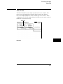
User’s Reference
Publication number 01660-97034
Second edition, January 2000
For Safety information, Warranties, and Regulatory
information, see the pages behind the index
 Copyright Agilent Technologies 1991 - 2000
All Rights Reserved
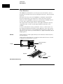
Agilent Technologies 1660A
Series 50/100-MHz State,
500-MHz Timing Logic
Analyzers
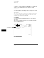
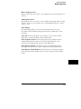
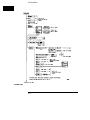
In This Book
The User’s Reference manual
contains field and feature definitions
which explain the details of the
instrument operation. Use this part
of the manual set for information on
what the menu fields do and what
they are used for. This manual
covers all 1660A Series analyzers.
The User’s Reference is divided into
two parts. The first part covers
general product information such as,
probing, using the front panel
interface, using the keyboard and
mouse, connecting a printer, disk
drive operation, the RS-232/GPIB/
Centronix interface, and the utilities
menu. The second part covers the
state and timing analyzers. It
explains the analyzer menus and
what they are used for. There are
separately tabbed chapters for each
analyzer menu, a chapter for error
messages, and a chapter for
instrument specifications. The
common menu fields which are found
in the majority of menus have been
placed in a separate chapter. You will
be referenced back to the "Common
Menu Fields" chapter when these
fields are encountered.
1
Introduction
2
Probing
3
Using the Front Panel Interface
4
Using the Optional
Keyboard and Mouse
5
Connecting a Printer
6
Disk Drive Operations
7
The RS-232/GPIB Interface
8
The Utilities Menu
9
The Common Menu Fields
10
The Configuration Menu
11
The Format Menu
12
The Trigger Menu
13
The Listing Menu
14
The Waveform Menu
15
The Mixed Display Menu
iii
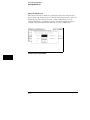
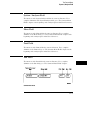
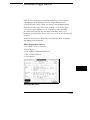
Analyzer type considerations
In the Configuration menu you have the choice of configuring an
analyzer machine as either a State analyzer or a Timing analyzer.
Some menus in the analyzer will change depending on the analyzer
type you choose. For example, since a Timing analyzer does not use
external clocks, the clock assignment fields in the Format menu will
not be available.
If a menu field is only available to a particular analyzer type, the field
is designated (Timing only) or (State only) after the field name. If no
designation is shown, the field is available for both types.
iv
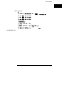
16
The Chart Menu
17
The Compare Menu
18
Error Messages
19
Specifications and
Characteristics
20
Operator’s Service
Index
v
vi
Contents
1 Introduction
User Interface 1–4
Configuration Capabilities 1–5
Key Features 1–7
Accessories Supplied 1–8
Accessories Available 1–9
2 Probing
General-Purpose Probing System Description 2–5
Assembling the Probing System 2–8
3 Using the Front-Panel Interface
Front-Panel Controls 3–3
Rear-Panel Controls and Connectors 3–8
How to Power-up The Analyzer 3–10
How to Select Menus 3–11
How to Select the System Menus 3–13
How to Select Fields 3–15
How to Configure Options 3–18
How to Enter Numeric Data 3–19
How to Enter Alpha Data 3–21
How to Roll Offscreen Data 3–23
How to Use Assignment/Specification Menus 3–25
4 Using the Mouse and the Optional Keyboard
Moving the Cursor 4–3
Entering Data into a Menu 4–4
Using the Keyboard Overlays 4–5
Defining Units of Measure 4–7
Assigning Edge Triggers 4–8
Closing a Menu 4–8
Contents - 1
Contents
5 Connecting a Printer
GPIB Printers 5–3
RS-232C Printers 5–8
Parallel Printers (1664A Only) 5–13
Connecting to Other Hewlett-Packard Printers 5–15
Printing the Display 5–17
6 Disk Drive Operations
How to Access the Disk Menu 6–5
How to Install a Disk 6–6
How to Select a Disk Operation 6–7
How to Load a File 6–8
How to Format a Disk 6–10
How to Store Files on a Disk 6–12
How to Rename a File 6–15
How to Autoload a File 6–17
How to Purge a File 6–19
How to Copy a File 6–20
How to Pack a Disk 6–22
How to Duplicate a Disk 6–23
How to Make a Directory 6–25
7 The RS-232C, GPIB, and Centronix Interface
The GPIB Interface 7–8
The RS-232C Interface 7–10
The Centronix Interface (1664A Only) 7–13
Configuring the Interface for a Controller or a Printer (1660A through 1663A
Only) 7–14
8 The System Utilities
Real Time Clock Adjustments (1660A Through 1663A Only) 8–4
Update FLASH ROM (1660A Through 1663A Only) 8–5
Display Grey Shade Adjustments 8–5
Sound On / Off 8–5
Contents - 2
Contents
9 The Common Menu Fields
System/Analyzer Field 9–4
Menu Field 9–5
Print Field 9–6
Run/Stop Field 9–9
Base Field 9–10
Label Field 9–11
Label / Base Roll Field 9–13
10 The Configuration Menu
Name Field 10–3
Type Field 10–4
Unassigned Pods List 10–5
Activity Indicators 10–7
System / Analyzer Field 10–8
Menu Field 10–8
Print Field 10–8
Run Field 10–8
11 The Format Menu
State Acquisition Mode Field (State only) 11–4
Timing Acquisition Mode Field (Timing only) 11–5
Clock Inputs Display 11–13
Pod Field 11–14
Pod Clock Field (State only) 11–15
Pod Threshold Field 11–19
Master and Slave Clock Field (State only) 11–21
Setup/Hold Field (State only) 11–23
Symbols Field 11–25
Label and Pod Rolling Fields 11–29
Label Assignment Fields 11–30
Label Polarity Fields 11–32
Bit Assignment Fields 11–33
System / Analyzer Field 11–35
Menu Field 11–35
Contents - 3
Contents
Print Field 11–35
Run Field 11–35
12 The Trigger Menu
Trigger Sequence Levels 12–6
Modify Trigger Field 12–8
Pre-defined Trigger Macros 12–11
Using Macros to Create a Trigger Specification 12–13
Timing Trigger Macro Library 12–14
State Trigger Macro Library 12–16
Modifying the User-level Macro 12–19
Resource Terms 12–26
Assigning Resource Term Names and Values 12–28
Label and Base Fields 12–32
Arming Control Field 12–33
Acquisition Control 12–36
Trigger Position Field 12–37
Sample Period Field 12–38
Branches Taken Stored / Not Stored Field 12–38
Count Field (State only) 12–39
13 The Listing Menu
Markers Field 13–4
Pattern Markers 13–5
Find X-pattern / O-pattern Field 13–6
Pattern Occurrence Fields 13–7
From Trigger / Start / X Marker Field 13–8
Specify Patterns Field 13–9
Contents - 4
Contents
Stop Measurement Field 13–13
Clear Pattern Field 13–16
Time Markers 13–17
Trig to X / Trig to O Fields 13–18
Statistics Markers 13–19
States Markers (State only) 13–21
Trig to X / Trig to O Fields 13–22
Data Roll Field 13–23
Label and Base Fields 13–24
Label / Base Roll Field 13–24
System / Analyzer Field 13–25
Menu Field 13–25
Print Field 13–25
Run Field 13–25
14 The Waveform Menu
Acquisition Control Field 14–5
Accumulate Field 14–6
States Per Division Field (State only) 14–7
Seconds Per Division Field (Timing only) 14–8
Delay Field 14–9
Sample Period Display (Timing only) 14–10
Markers Field 14–12
Pattern Markers 14–13
X-pat / O-pat Occurrence Fields 14–14
From Trigger / Start / X Marker Field 14–15
X to O Display Field (Timing only) 14–16
Center Screen Field 14–17
Specify Patterns Field 14–18
Stop Measurement Field 14–22
Clear Pattern Field 14–25
Contents - 5
Contents
Time Markers 14–26
Trig to X / Trig to O Fields 14–27
Marker Label / Base and Display 14–28
Statistics Markers 14–29
States Markers (State only) 14–31
Trig to X / Trig to O Fields 14–32
Marker Label / Base and Display 14–33
Waveform Display 14–34
Waveform Label Field 14–36
System / Analyzer Field 14–39
Menu Field 14–39
Print Field 14–39
Run Field 14–39
15 The Mixed Display Menu
Inserting Waveforms 15–3
Interleaving State Listings 15–3
Time-Correlated Displays 15–4
Markers 15–5
16 The Chart Menu
Selecting the Axes for the Chart 16–6
Y-axis Label Value Field 16–7
X-axis Label / State Type Field 16–8
Scaling the Axes 16–9
Min and Max Scaling Fields 16–10
Markers / Range Field 16–11
Contents - 6
Contents
Pattern Markers 16–12
Find X-pattern / O-pattern Field 16–13
Pattern Occurrence Fields 16–14
From Trigger / Start / X-Marker Fields 16–15
Specify Patterns Field 16–16
Stop Measurement Field 16–19
Clear Pattern Field 16–22
Time Markers 16–23
Trig to X / Trig to O Fields 16–24
Statistics Markers 16–25
States Markers 16–27
Trig to X / Trig to O Fields 16–28
System / Analyzer Field 16–29
Menu Field 16–29
Print Field 16–29
Run Field 16–29
17 The Compare Menu
Reference Listing Field 17–5
Difference Listing Field 17–6
Copy Listing to Reference Field 17–8
Find Error Field 17–9
Compare Full / Compare Partial Field 17–10
Mask Field 17–11
Specify Stop Measurement Field 17–12
Data Roll Field 17–15
Bit Editing Field 17–16
Label and Base Fields 17–17
Label / Base Roll Field 17–17
System / Analyzer Field 17–18
Menu Field 17–18
Contents - 7
Contents
Print Field 17–18
Run Field 17–18
18 Error Messages
Error Messages 18–3
Warning Messages 18–5
Advisory Messages 18–8
19 Specifications and Characteristics
Specifications 19–3
Specifications and Characteristics 19–4
20 Operator’s Service
Preparing For Use 20–3
To inspect the logic analyzer 20–4
Ferrites (1664A Only) 20–4
To apply power 20–6
To operate the user interface 20–6
To set the line voltage 20–7
To degauss the display 20–8
To clean the logic analyzer 20–8
To test the logic analyzer 20–8
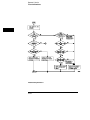
Troubleshooting 20–9
To use the flowcharts 20–9
To check the power-up tests 20–12
To run the self-tests (1660A through 1663A) 20–13
To run the self-tests (1664A) 20–19
To test the auxiliary power 20–26
Contents - 8
1
Introduction
Logic Analyzer Description
The Agilent Technologies 1660A Series Logic Analyzers are part of a
new generation of general-purpose logic analyzers. The 1660A Series
consists of five different models ranging in channel width from 34
channels to 136 channels. State speed is either 50-MHz or 100-MHz
(depending on the model), and all models have 500-MHz timing
speeds. The 1660A series logic analyzers are designed as full-featured
stand-alone instruments for use by digital and microprocessor
hardware and software designers. All models have GPIB, RS-232C,
and/or Centronix interfaces for hard copy printouts and control by a
host computer.
• The 1660A has 100-MHz state speed, 130 data channels, six
data/clock channels, and both GPIB/RS-232C interfaces.
• The 1661A has 100-MHz state speed, 96 data channels, six
data/clock channels, and both GPIB/RS-232C interfaces.
• The 1662A has 100-MHz state speed, 64 data channels and four
data/clock channels, and both GPIB/RS-232C interfaces.
• The 1663A has 100-MHz state speed, 32 data channels, two
data/clock channels, and both GPIB/RS-232C interfaces.
• The 1664A has 50-MHz state speed, 32 data channels, two
data/clock channels, and a Centronix interface (GPIB/RS-232C
available as options).
Memory depth is 4 Kbytes per channel in all pod pair groupings, or
8 Kbytes per channel on one pod of a pod pair (half channel mode).
Measurement data is displayed as data listings and waveforms, and
can also be plotted on a chart or compared to a reference image.
The 50/100-MHz state analyzer has master, master/slave, and
demultiplexed clocking modes available. Measurement data can be
stamped with state or time tags. For triggering and data storage, the
state analyzer uses 12 sequence levels with two-way branching, 10
pattern resource terms, 2 range terms, and 2 timers.
1–2
Introduction
The 500-MHz timing analyzer has conventional, transitional, and glitch
timing modes with variable width, depth, and speed selections.
Sequential triggering uses 10 sequence levels with two-way branching,
10 pattern resource terms, 2 range terms, 2 edge terms and 2 timers.
1–3
Introduction
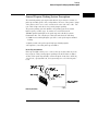
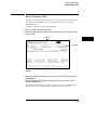
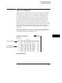
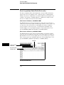
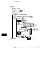
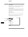
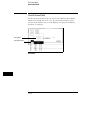
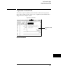
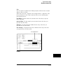
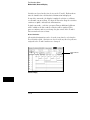
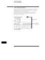
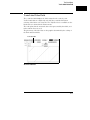
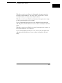
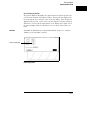
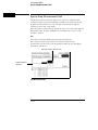
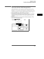
User Interface
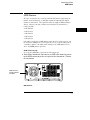
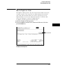
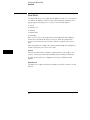
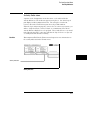
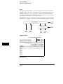
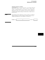
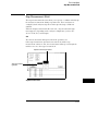
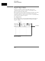
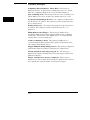
User Interface
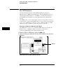
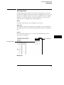
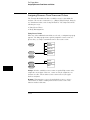
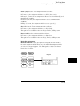
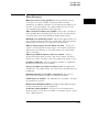
The 1660 Series analyzers have several easy-to-use user interface devices:
the knob, the front panel arrow keys and keypad, the mouse, and the optional
keyboard.
Front panel arrow keys move the highlighter to identify the desired field,
then a front panel Select key is pressed to activate the field. The knob
quickly moves the highlighter (cursor) in certain menus to highlight options
to select and to quickly change numeric assignment fields.
The keypad on the front panel is used to enter alpha and numeric data into
assignment fields. A mouse and an optional full size keyboard are also
available.
To select a field with the mouse, position the cursor (+) of the mouse over
the desired field and press the button on the upper-left corner of the mouse.
The optional keyboard can control all instrument functions by using special
function keys, the arrow keys, and the Enter key. Alpha and numeric entry is
simply typed in.
See Also
"Using the Mouse and the Optional Keyboard" found later in this manual for
more information.
"Using the Front-Panel Interface" found later in this manual for more details
on using the standard interface devices.
Alpha and numeric
keypads
Display
Knob
Keyboard
Mouse
Front-Panel Interface Devices
1–4
Introduction
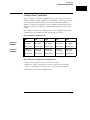
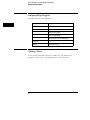
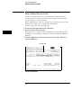
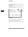
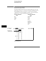
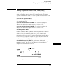
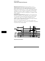
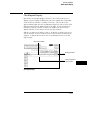
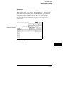
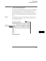
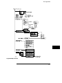
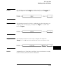
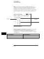
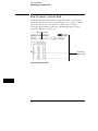
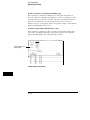
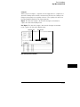
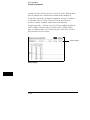
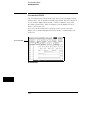
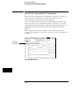
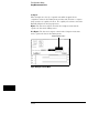
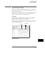
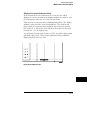
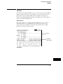
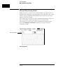
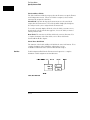
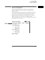
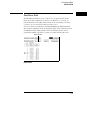
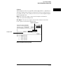
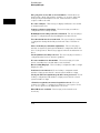
Configuration Capabilities
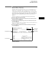
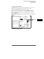
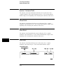
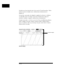
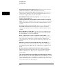
Configuration Capabilities
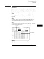
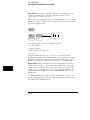
The five analyzer models in the 1660 Series offer a wide variety of channel
widths and memory depth combinations. The number of data channels range
from 34 channels with the 1664A, up to 136 channels with the 1660A. In
addition, a half channel acquisition mode is available which doubles memory
depth from 4 Kbytes to 8 Kbytes per channel while reducing channel width
by half.
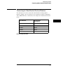
The configuration guide below illustrates the memory depth/channel width
combinations in all acquisition modes with all analyzer models.
State Analyzer Configurations
Half channel
50/100 MHz
Full channel
50/100 MHz
1660A
1661A
1662A
1663A
1664A
8K-deep / 68
chan. 65 data
+
3 data or clock
8K-deep / 51
chan. 48 data
+
3 data or clock
8K-deep / 34
chan. 32 data
+
2 data or clock
8K-deep / 17
chan. 16 data
+
1 data or clock
8K-deep / 17
chan. 16 data
+
1 data or clock
4K-deep / 136
chan. 130 data
+
6 data or clock
4K-deep / 102
chan. 96 data
+
6 data or clock
4K-deep / 68
chan. 64 data
+
4 data or clock
4K-deep / 34
chan. 32 data
+
2 data or clock
4K-deep / 34
chan. 32 data
+
2 data or clock
State Analyzer Configuration Considerations
• Unused clock channels can be used as data channels.
• With Time or State tags turned on, memory depth is reduced by half.
However, full depth is retained if you leave one pod pair unassigned.
• Maximum of 6 clocks in the 1660A model.
1–5
Introduction
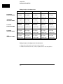
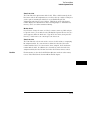
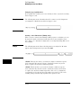
Configuration Capabilities
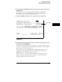
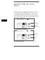
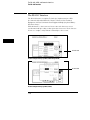
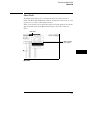
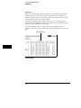
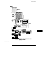
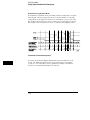
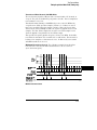
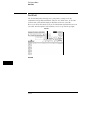
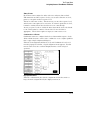
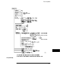
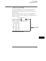
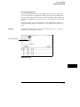
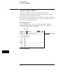
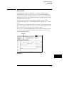
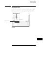
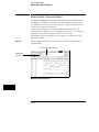
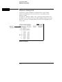
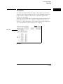
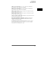
Timing Analyzer Configurations
1660A
1661A
1662A
1663A
1664A
8K-deep / 68
chan. 65 data
+
3 data or clock
8K-deep / 51
chan. 48 data
+
3 data or clock
8K-deep / 34
chan. 32 data
+
2 data or clock
8K-deep / 17
chan. 16 data
+
1 data or clock
8K-deep / 17
chan. 16 data
+
1 data or clock
Conventional
full channel 250 MHz
4K-deep / 136
chan. 130 data
+
6 data or clock
4K-deep / 102
chan. 96 data
+
6 data or clock
4K-deep / 68
chan. 64 data
+
4 data or clock
4K-deep / 34
chan. 32 data
+
2 data or clock
4K-deep / 34
chan. 32 data
+
2 data or clock
Transitional
half channel 250 MHz
8K-deep / 68
chan. 65 data
+
3 data or clock
8K-deep / 51
chan. 48 data
+
3 data or clock
8K-deep / 34
chan. 32 data
+
2 data or clock
8K-deep / 17
chan. 16 data
+
1 data or clock
8K-deep / 17
chan. 16 data
+
1 data or clock
Transitional
full channel 125 MHz
4K-deep / 136
chan. 130 data
+
6 data or clock
4K-deep / 102
chan. 96 data
+
6 data or clock
4K-deep / 68
chan. 64 data
+
4 data or clock
4K-deep / 34
chan. 32 data
+
2 data or clock
4K-deep / 34
chan. 32 data
+
2 data or clock
Glitch
half channel 125 MHz
4K-deep / 68
chan. 65 data
+
3 data or clock
4K-deep / 51
chan. 48 data
+
3 data or clock
4K-deep / 34
chan. 32 data
+
2 data or clock
4K-deep / 17
chan. 16 data
+
1 data or clock
4K-deep / 17
chan. 16 data
+
1 data or clock
Conventional
half channel 500 MHz
Timing Analyzer Configuration Considerations
• Unused clock channels can be used as data channels
• In Glitch half channel mode, memory is split between data and glitches.
1–6
Introduction
Key Features
Key Features
Key features of the 1660A Series are listed below:
Analyzers
• 50-MHz (1664A) or 100-MHz state (1660A through 1663A), and 500-MHz
timing acquisition speed.
• Variety of channel widths ranging from 34 channels with the 1664A, up to
136 channels with the 1660A.
• Lightweight, passive probes for easy hookup and compatibility with
previous Agilent logic analyzers and preprocessors.
• GPIB and RS-232C interfaces (1660A through 1663A) or Centronix
interface (1664A) for programming and hard copy printouts (GPIB and
RS-232C interfaces are optional on the 1664A).
• Variable setup/hold time in the State analyzer.
• External triggering to/from other instruments through rear-panel BNCs.
• 4 Kbytes-deep memory on all channels with 8 Kbytes-deep in half channel
modes.
• Marker measurements.
• Pre-configured trigger macros. 12 levels of trigger sequencing for state
and 10 levels of sequential triggering for Timing.
• Both state and timing analyzers can use 10 pattern resource terms,
2 range terms, and 2 timer/counters to qualify and trigger on data. In
addition, the timing analyzer has 2 edge terms.
• 50-MHz (1664A) or 100-MHz (1660A through 1663A) time and
number-of-states tagging.
• Full programmability.
• State/State and mixed State/Timing displays.
• Compare, Chart, and Waveform displays.
1–7
Introduction
Accessories Supplied
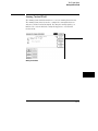
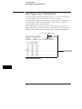
Accessories Supplied
The table below lists the accessories supplied with your logic analyzer. If any
of these accessories are missing, contact your nearest Agilent Technologies
sales office.
Accessories
Quantity
Probe tip assemblies
Note 1
Quick Start Training Kit
1*
Programming Reference
1*
Probe cables
Note 2
Grabbers (20 per pack)
Note 1
Extra probe leads (5 per pack)
Note 3
Operating system disks
1 (Note 4)
User’s Reference
1
Accessories pouch
1
Mouse
1
Note 1 Quantities :
8 - 1660A
6 - 1661A
4 - 1662A
2 - 1663A and 1664A
Note 2 Quantities :
4 - 1660A
3 - 1661A
2 - 1662A
1 - 1663A and 1664A
Note 3 Quantities :
8 - 1660A
6 - 1661A
4 - 1662A
2 - 1663A
0 - 1664A
Note 4 The 1664A requires an Operating System disk for turn-on and boot-up.
Operation of the analyzer is not possible without this disk.
* Standard equipment (or supplied accessory) for all models except the 1664A. Items can be
ordered as an option for the 1664A.
See Also
Accessories for Agilent Logic Analyzers if you need additional accessories.
1–8
Introduction
Accessories Available
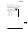
Accessories Available
There are a number of accessories available that will make your measurement
tasks easier and more accurate. You will find these listed in Accessories for
Agilent Logic Analyzers. The table below lists additional documentation
that is available from your nearest Agilent Technologies sales office for use
with your logic analyzer.
Accessories Available
Quantity
Quick Start Training Kit
1*
Programming Reference
1*
Service Guide
1
* Standard equipment for all models except the 1664A. Items can be ordered as an option for the
1664A.
Preprocessor Modules
The preprocessor module accessories enable you to quickly and easily
connect the logic analyzer to your microprocessor under test.
Included with each preprocessor module is a 3.5-inch disk which contains a
configuration file and an inverse assembler file. When you load the
configuration file, it configures the logic analyzer for making state
measurements on the microprocessor for which the preprocessor is designed.
Configuration files from other analyzers can also be loaded. For information
on translating other configuration files into the analyzer, refer to the
applicable preprocessor manual.
The inverse assembler file is a software routine that will display captured
information in a specific microprocessor’s mnemonics. The DATA field in the
State Listing is replaced with an inverse assembly field. The inverse
assembler software is designed to provide a display that closely resembles
the original assembly language listing of the microprocessor’s software. It also
identifies the microprocessor bus cycles captured, such as Memory Read,
Interrupt Acknowledge, or I/O Write.
Many of the preprocessor modules require the Agilent Technologies 10269C
General-Purpose Probe Interface. The probe interface accepts the specific
preprocessor PC board and connects it to five connectors on the
general-purpose interface to which the logic analyzer probe cables connect.
1–9
Introduction
Accessories Available
See Also
Accessories for Logic Analyzers for a list of preprocessor modules and their
descriptions.
1–10
2
Probing
Probing
This chapter contains a description of the probing system for the logic
analyzer. It also contains the information you need for connecting the
probe system components to each other, to the logic analyzer, and to
the system under test.
Probing Options
You can connect the logic analyzer to your system under test in one of
the following ways:
•
•
•
•
Agilent Technologies 10320C User-Definable Interface (optional).
Microprocessor and bus specific interfaces (optional).
Standard general-purpose probing (provided).
Direct connection to a 20-pin, 3M-Series type header connector
using the optional termination adapter.
The 10320C User-Definable Interface
The optional 10320C User-Definable Interface module combined with
the optional Agilent Technologies 10269C General Purpose Probe
Interface allows you to connect the logic analyzer to the
microprocessor in your target system. The 10320C includes a
breadboard that you custom wire for your system.
Another option for use with the interface module is the Agilent
Technologies 10321A Microprocessor Interface Kit. This kit includes
sockets, bypass capacitors, and a fuse for power distribution. Also
included are wire-wrap headers to simplify wiring of your interface
when you need active devices to support the connection requirements
of your system.
See Also
Accessories for Agilent Logic Analyzers for additional information
about the interface module and the microprocessor interface kits.
2–2
Probing
Microprocessor and Bus Specific Interfaces
There are a number of microprocessor and bus specific interfaces
available as optional accessories that are listed in the Accessories for
Agilent Logic Analyzers. Microprocessors are supported by
Universal Interfaces or Preprocessor Interfaces, or in some cases, both.
Universal Interfaces are aimed at initial hardware turn-on, and will
provide fast, reliable, and convenient connections to the
microprocessor system.
Preprocessor interfaces are aimed at hardware turn-on and
hardware/software integration, and will provide the following:
• All clocking and demultiplexing circuits needed to capture the
system’s operation.
• Additional status lines to further decode the operation of the CPU.
• Inverse assembly software to translate logic levels captured by the
logic analyzer into microprocessor mnemonics.
Bus interfaces will support bus analysis for the following:
• Bus support for GPIB, RS-232C, RS-449, SCSI, VME, and VXI.
General-Purpose Probing
General-purpose probing involves connecting the logic analyzer
probes directly to your target system without using any interface.
General-purpose probing does not limit you to specific hookup
schemes, for an example, as the probe interface does.
General-purpose probing uses grabbers that connect to both through
hole and surface mount components. General-purpose probing comes
as the standard probing option. You will find a full description of its
components and use later in this chapter.
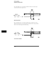
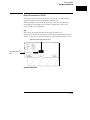
The Termination Adapter
The optional termination adapter allows you to connect the logic
analyzer probe cables directly to test ports on your target system
without the probes.
2–3
Probing
The termination adapter is designed to connect to a 20 (2x10)
position, 4-wall, low-profile, header connector which is a 3M-Series
3592 or equivalent.
Termination Adapter
2–4
Probing
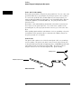
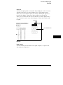
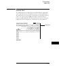
General-Purpose Probing System Description
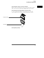
General-Purpose Probing System Description
The standard probing system provided with the logic analyzer consists of a
probe tip assembly, probe cable, and grabbers. Because of the passive design
of the probes, there are no active circuits at the outer end of the cable. The
rest of this chapter is dedicated to general-purpose probing.
The passive probing system is similar to the probing system used with
high-frequency oscilloscopes. It consists of a series RC network
(90 kΩ in parallel with 8 pF) at the probe tip, and a shielded, resistive
transmission line. The advantages of this system include the following:
• 250 Ω in series with 8-pF input capacitance at the probe tip for minimal
loading.
• Signal ground at the probe tip for high-speed timing signals.
• Inexpensive, removable probe tip assemblies.
Probe Tip Assemblies
Probe tip assemblies allow you to connect the logic analyzer directly to the
target system. This general-purpose probing is useful for discrete digital
circuits. Each probe tip assembly contains 16 probe leads (data channels),
1 clock lead, a pod ground lead, and a ground tap for each of the 16 probe
leads.
Probe Tip Assembly
2–5
Probing
General-Purpose Probing System Description
Probe and Pod Grounding
Each pod is grounded by a long, black, pod ground lead. You can connect the
ground lead directly to a ground pin on your target system or use a grabber.
To connect the ground lead to grounded pins on your target system, you
must use 0.63-mm (0.025-in) square pins, or use round pins with a diameter
of 0.66 mm (0.026 in) to 0.84 mm (0.033 in). The pod ground lead must
always be used.
Each probe can be individually grounded with a short black extension lead
that connects to the probe tip socket. You can then use a grabber or the
grounded pins on your target system in the same way you connect the data
lines.
When probing signals with rise and fall times of ≤ 1 ns, grounding each probe
lead with the 2-inch ground lead is recommended. In addition, always use
the probe ground on a clock probe.
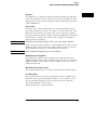
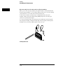
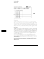
Probe Leads
The probe leads consists of one 12-inch, twisted-pair cable; one ground tap;
and one grabber. The probe lead, which connects to the target system, has
an integrated RC network with an input impedance of 100 kΩ in parallel with
approximately 8 pF, and all in series with 250 Ω. The probe lead has a
two-pin connector on one end that snaps into the probe housing.
Probe ground
Probe lead connector
Probe Ground Lead
2–6
Probing
General-Purpose Probing System Description
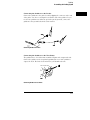
Grabbers
The grabbers have a small hook that fits around the IC pins and component
leads. The grabbers have been designed to fit on adjacent IC pins on either
through hole or surface mount components with lead spacing greater than or
equal to 0.050 inches.
Probe Cable
The probe cable contains 18 signal lines, 17 chassis ground lines and two
power lines for preprocessor use. The cables are woven together into a flat
ribbon that is 4.5 feet long. The probe cable connects the logic analyzer to
the pods, termination adapter, Agilent Technologies 10269C General-Purpose
Probe Interface, or preprocessor. Each cable is capable of carrying 0.33
amps for preprocessor power.
CAUTION
DO NOT exceed this 0.33 amps per cable or the cable will be damaged.
Preprocessor power is protected by a current limiting circuit. If the current
limiting circuit is activated, the fault condition must be removed. After the
fault condition is removed, the circuit will reset in one minute.
NOTE
1663A and 1664A analyzers use the same pod labels.
Minimum Signal Amplitude
Any signal line you intend to probe with the logic analyzer probes must
supply a minimum voltage swing of 500 mV to the probe tip. If you measure
signal lines with a voltage swing of less than 500 mV, you may not obtain a
reliable measurement.
Maximum Probe Input Voltage
The maximum input voltage of each logic analyzer probe is ±40 volts peak.
Pod Thresholds
Logic analyzer pods have two preset thresholds and a user-definable pod
threshold. The two preset thresholds are ECL (−1.3 V) and TTL (+1.5 V).
The user-definable threshold can be set anywhere between −6.0 volts
and +6.0 volts in 0.05 volt increments.
All pod thresholds are set independently.
2–7
Probing
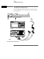
Assembling the Probing System
Assembling the Probing System
The general-purpose probing system components are assembled as shown to
make a connection between the measured signal line and the pods displayed
in the Format menu.
Connecting Probe Cables to the Logic Analyzer
2–8
Probing
Assembling the Probing System
Connecting Probe Cables to the Logic Analyzer
All probe cables are installed at the factory. If you need to replace a probe
cable, refer to the Service Guide that is supplied with the logic analyzer.
Connecting the Probe Tip Assembly to the Probe Cable
To connect a probe tip assembly to a cable, align the key on the cable
connector with the slot on the probe housing and press them together.
Probe tip assembly
Probe cable
Connecting Probe Tip Assembly
2–9
Probing
Assembling the Probing System
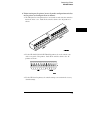
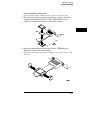
Disconnecting Probe Leads from Probe Tip Assemblies
When you receive the logic analyzer, the probe leads are already installed in
the probe tip assemblies. To keep unused probe leads out of your way during
a measurement, you can disconnect them from the pod.
To disconnect a probe, insert the tip of a ball-point pen into the latch
opening. Push on the latch while gently pulling the probe out of the pod
connector as shown in the figure.
To connect the probes into the pods, insert the double pin end of the probe
into the probe housing. Both the double pin end of the probe and the probe
housing are keyed so they will fit together only one way.
Installing Probe Leads
2–10
Probing
Assembling the Probing System
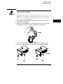
Connecting the Grabbers to the Probes
Connect the grabbers to the probe leads by slipping the connector at the end
of the probe onto the recessed pin located in the side of the grabber. If you
need to use grabbers for either the pod or the probe grounds, connect the
grabbers to the ground leads in the same manner.
Connecting Grabbers to Probes
Connecting the Grabbers to the Test Points
The grabbers have a hook that fits around the IC pins and component leads.
Connect the grabber to the test point by pushing the rear of the grabber to
expose the hook. Hook the lead and release your thumb as shown.
Connecting Grabbers to Test Points
2–11
Probing
Assembling the Probing System
2–12
3
Using the Front-Panel Interface
The Front-Panel Interface
This chapter explains how to use the front-panel user interface. The
front and rear-panel controls and connectors are explained in the first
part of this chapter followed by a series of "How to Use" examples.
The front-panel interface consists of front-panel keys, a knob, and a
display. The interface allows you to configure the instrument by
moving between menus and setting parameters within the menus.
The interface then displays the measurement results. In general,
using the front-panel interface involves the following processes:
• Selecting the desired menu with the MENU keys.
• Placing the cursor on the desired field by using the arrow keys and
by rotating the knob.
• Selecting and displaying the field options or current data by
pressing the Select key.
• If necessary, selecting lower level options or entering new data by
using the knob, arrow keys, or the keypad.
• Starting and stopping data acquisition by using the Run and Stop
keys.
If you want to step through the examples on using the interface,
simply turn the power Off, then back On. Start with the section,
"How to Select Menus."
3–2
Using the Front-Panel Interface
Front-Panel Controls
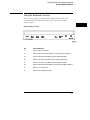
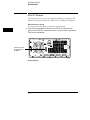
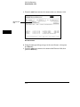
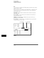
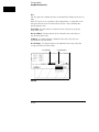
Front-Panel Controls
In order to apply the user interface quickly, you should know what the
following front-panel controls do.
Clear entry key
Don’t Care key
+/- key
. key
Hexadecimal
keypad
Menu keys
Run/Continue
key
Stop key
Select/Done keys
Arrow keys
Print/All
key
Knob
Page keys
Front-Panel Layout
Cursor
Shift key
Alpha keypad
The Cursor
The cursor (inverse video field) highlights interactive fields within the menus
that you want to use. Interactive fields are enclosed in boxes in each menu.
When you press the arrow keys, the cursor moves from one field to another.
MENU Keys
The menu keys allow you to quickly select the main menus in the logic
analyzer. These keys are System, Config, Format, Trigger, List, and
Waveform. The System key accesses the system menu. The Config, Format,
Trigger, List, and Waveform keys will display the menus of either analyzer
(machine) 1 or 2 respectively depending on what menu was last displayed.
3–3
Using the Front-Panel Interface
Front-Panel Controls
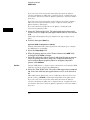
System Menu Key The System key allows you to access the System
subset menus. The subset menus are the Disk, RS-232 / GPIB
(Printer/Controller for 1664A), Utilities, and Test menus.
Config Menu Key The Config menu key allows you to access either
the Timing or State Configuration menu. You exit the Config menu by
pressing another menu key.
Format Menu Key The Format menu key allows you to access either
the Timing or State Format menu. You exit the Format/Display menu by
pressing another menu key.
Trigger Menu Key The Trigger menu key allows you to access either
the Timing or State Trigger menu. You exit the Trigger menu by
pressing another menu key.
List Menu Key The List menu key allows you to access either the
Timing or State Listing menu. In addition, if the List key is pressed a
second time, the Compare menu becomes available. The available menus
depend on the type of analyzers turned on and what analyzer was
accessed last. You exit the List menu by pressing another menu key.
Waveform Menu Key The Waveform menu key allows you to access
either the Timing or State Waveform menu. In addition, if the Waveform
key is pressed a second time, the Chart menu becomes available. The
available menus depends on the type of analyzers turned on and what
analyzer was accessed last. You exit the Waveform menu by pressing
another menu key.
Select Key
The Select key initiates an interface action that is dictated by the field
currently highlighted. The highlighted field could be an option field within a
pop-up, a toggle field, an assignment field, or a Done field. For example, if
the field is a Done field, you just press the Select key to finish that task.
When option fields are selected, they either save the highlighted selection
into the configuration, or they access other pop-ups requiring another
selection or assignment. When you select an option, the pop-up either closes
automatically with the Select key or it closes when you select the Done field.
When toggle fields are selected, the field will automatically switch to the
other choice.
3–4
Using the Front-Panel Interface
Front-Panel Controls
When you select an assignment field, it opens. When the Select key is
pressed in an opened assignment field, either a highlighted option is
assigned, or keypad entries are assigned. Then the assignment field closes.
Done Key
The Done key stops any field selection and assignment actions by saving the
current selections and closing the opened pop-up. In some fields, its action is
the same as the Select key.
Arrow Keys
The arrow keys move the cursor around the menu in a horizontal and vertical
direction, according to the direction of the arrow.
Knob
The knob has four major functions, depending on what field or pop-up menu
you are in. The knob allows you to do the following:
• Increment/decrement numeric values in numeric pop-up menus.
• Roll the offscreen display containing such things as data listings,
waveforms, the resource term list, sequence level list, or labels. Depending
on what display is rolled, the direction can be left, right, up, or down.
• Move the cursor from option to option within a selection list.
• Move the cursor from field to field within an assignment field.
Page Keys
The Page keys roll offscreen display data such as pods, labels, resource
terms, data listings, and waveforms one screen at a time. To roll data in an
up and down direction, press the up or down Page keys. To roll data in a left
to right direction, press the blue shift key prior to the left or right Page key.
When the blue shift key is pressed followed by a left or right arrow key, only
one page roll occurs. For multiple left or right paging, you must repeat the
two-key process.
If there are multiple items in a menu that need paging, the field containing
the item name turns dark indicating it is rollable. The Page keys work
independant of the knob. If there are up and down rollable data, simply press
the up or down front-panel Page keys. If there are left and right rollable data,
press the blue shift key, then the left or right Page key (Shift+Page). This
two-key sequence is repeated for each paged screen.
3–5
Using the Front-Panel Interface
Front-Panel Controls
Run/Rep Key
The Run key starts a data acquisition in any run mode you specify. After the
acquisition, the analyzer (state or timing) is automatically forced into the last
display menu accessed.
To start a single run, press the Run/Rep key. To start a Repetitive run, press
the blue shift key, then press the Run/Rep key.
Stop key
The Stop key allows you to stop data acquisition or printing. After the
acquisition is stopped, the data displayed onscreen depends on which run
mode (single or repetitive) was used to acquire the data. In the repetitive
mode, Stop halts acquisition after the last completed single acquisition cycle.
In single mode, Stop causes the single data acquisition to be aborted and
partial data is displayed. If you print a hard copy, the Stop key stops the print.
Print/All Key
The Print/All key starts a hard copy print of the screen and any data that
appears on that screen. To print all data that is offscreen, press the blue shift
key prior to pressing the Print/All key.
Don’t Care Key
The Don’t Care key allows you to enter don’t cares (Xs) in binary, octal, and
hexadecimal pattern assignment fields. In Alpha Entry fields, this key enters
a space and moves the underscore marker to the next space.
Clear Entry Key
The Clear entry key allows you to clear assignment fields of alpha entries,
channel assignments, and numeric entries. When you press the Clear entry
key in an alpha assignment field, a cursor appears that indicates the start
point for new alpha entry.
± Key
The ± key allows you to change the sign (±) of numeric variables.
. (period) Key
The period key allows you to enter a period in a numeric entry, turn off a
channel assignment, or enter a period in an alpha assignment.
3–6
Using the Front-Panel Interface
Front-Panel Controls
Hexadecimal Keypad
The hexadecimal keypad allows you to enter numeric values in numeric entry
fields. You enter values in the four number bases Binary, Octal, Decimal, and
Hexadecimal. The A through F keys are used for both hexadecimal and alpha
character entries.
Alpha Keypad
The alpha keypad allows you to enter letters in alpha entry fields. You enter
letters in fields where a custom name is desired.
Disk Drive
The disk drive is a 3.5 inch, double-sided, double density drive. Besides
loading the operating system, it allows you to store and load logic analyzer
configurations and inverse assembler files. There is a disk eject button
located on the right side. Press this button to eject a flexible disk from the
disk drive. The disk drive also has an indicator light. This light is illuminated
when the disk drive is operating. Wait until this light is out before removing
or inserting disks.
On 1664A analyzers, the operating system is not contained on ROM inside of
the unit, and MUST be loaded from disk when the 1664A is powered up.
Simply insert the operating system disk into the disk drive, then set the LINE
switch to ON.
3–7
Using the Front-Panel Interface
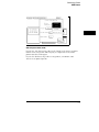
Rear-Panel Controls and Connectors
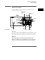
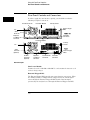
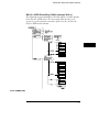
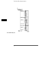
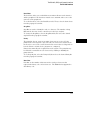
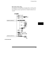
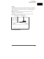
Rear-Panel Controls and Connectors
In order to apply the user interface quickly, you should know what the
following rear-panel controls do:
RS-232C Connector
Line Power Module
Intensity Control
External Trigger
BNCs
Fan
GPIB
Connector
Pod Cable
Connectors
Keyboard
and Mouse
Connector
Line Power Module
Intensity
Control
Fan
GPIB
Connector
(Optional)
External Trigger
BNCs
RS-232C
Connector
(Optional)
Keyboard
and Mouse
Connector
Parallel Printer
Connector
Pod Cable
Connector
Rear Panel Layout
Line Power Module
Permits selection of 110-120 or 220-240 Vac and contains the fuses for each
of these voltage ranges.
External Trigger BNCs
The External Trigger BNCs provide arm out and arm in connections. When
the Arming Control is configured in the Trigger menu, the Arm In signal
enters through the External Trigger In BNC and the Arm Out signal
generated by the analyzer leaves through the External Trigger Out BNC.
3–8
Using the Front-Panel Interface
Rear-Panel Controls and Connectors
Intensity Control
Allows you to set the display brightness to a comfortable level.
Pod Cable Connectors
These are keyed connectors for connecting the pod cables. Depending on
the analyzer model, you will see a different number of pod cables.
RS-232C Connector
Standard DB-25 type connector for connecting an RS-232C printer or
controller. This interface is standard on the 1660A through 1663A, and
optional on the 1664A.
GPIB Connector
Standard GPIB connector for connecting an GPIB printer or controller. This
interface is standard on the 1660A through 1663A, and optional on the 1664A.
Parallel Printer Port Connector
Standard DB-25 type connector for connecting a Centronix printer to the
1664A. This interface is not available on the 1660A through 1663A.
Keyboard and Mouse Connector
Standard keyboard/mouse connector for connecting an optional keyboard
and/or mouse.
Fan
Provides cooling for the logic analyzer. Make sure air is not restricted from
the fan and rear-panel openings.
3–9
Using the Front-Panel Interface
How to Power-up The Analyzer
How to Power-up The Analyzer
The method for powering up the analyzer is dependent on the model.
For the 1660A through 1663A, simply set the front panel LINE switch to ON.
Power On Procedure
For the 1664A, proceed as follows:
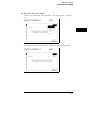
1 Insert the Operating System disk into the disk drive.
2 Set the front panel LINE switch to ON.
3 Verify "Loading System File" is displayed. If "System Disk Not
Found" is displayed, repeat procedure using the correct Operating
System disk.
NOTE
It is recommended that a working copy of the master Operating System disk
be made (using the "Duplicate Disk" function in the System Menu) and used
for normal operation. Place the master Operating System disk in a safe
location, for use when the working copy is damaged or lost.
3–10
Using the Front-Panel Interface
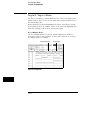
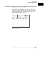
How to Select Menus
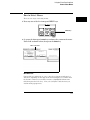
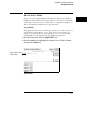
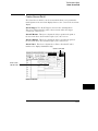
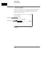
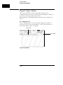
How to Select Menus
There are two ways of selecting menus.
1 Press any one of the five front-panel MENU keys.
MENU keys
2 Or, press the front-panel arrow keys and move the cursor to the menu
Name field as shown below, then press the Select key.
Menu name field
Menu Name Field
If more than one analyzer is on, you see the selected menu of analyzer 1 or
analyzer 2 depending on what type menu was last displayed. To switch from
the machine 1 menu set to machine 2 menu set, highlight the Menu name
field, then press the Select key. Now, select analyzer 2 and the menu you
want from the pop-up menu.
3–11
Using the Front-Panel Interface
How to Select Menus
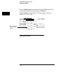
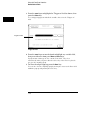
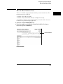
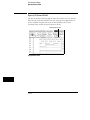
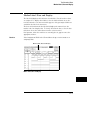
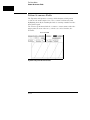
3. Press the Up/Down arrow keys or turn the knob to highlight the desired
menu name as shown below, then press the Select key.
In many applications, both analyzers are turned on. In these cases, if a
front-panel MENU key is pressed twice, all corresponding menus for that
MENU key become available.
Menu selection list
(not shown on the
1664A)
Complete Menu Selection List
3–12
Using the Front-Panel Interface
How to Select the System Menus
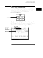
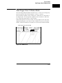
How to Select the System Menus
One of the six MENU keys is the System key. You use the System key to
access a set of menus that are used to configure system level parameters for
the I/O bus, clock, display, and the disk drive operations. To access the
menus under the System key, perform the following steps:
1 Press the System MENU key.
System key
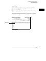
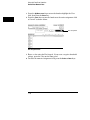
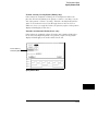
2 Press the arrow keys to highlight the menu Name field, then press the
Select key.
3 Press the Up/Down arrow keys or turn the knob to highlight the desired
System menu name as shown below, then press the Select key.
Menu name field
1660A through
1663A shown.
1664A displays
"Printer/Controller"
System menu
Selection List
System Menus Selection List
3–13
Using the Front-Panel Interface
How to Select the System Menus
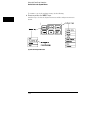
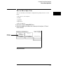
To return to one of the analyzer menus, do the following:
4 Press any of the five MENU keys.
Another way to look at the System menu set and the analyzer menu set is
shown.
System and Analyzer Menu Sets
3–14
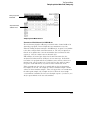
Using the Front-Panel Interface
How to Select Fields
How to Select Fields
The process of selecting individual fields within the main menus is simply to
highlight the desired field and then press the Select key. However, depending
on what type of field you select, you will either see a pop-up menu appear, or
will see an immediate assignment in a toggle type field.
Pop-up Menus
The pop-up menu is the most common type of menu you see when you select
a field. When a pop-up appears, you see a list of two or more options. The
pop-up closes after at least one of the options are selected. The following
example guides you through field selection within a pop-up menu.
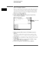
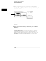
1 Press the front panel analyzer Trigger MENU key.
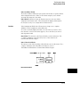
2 Press the arrow keys to highlight the sequence level 1 field as shown,
then press the Select key.
Timing sequence level
number 1 field
Sequence Level 1
3–15
Using the Front-Panel Interface
How to Select Fields
3 Press the arrow keys to highlight the "Trigger on" field as shown, then
press the Select key.
A second pop-up appears with all the variable choices for the "Trigger on"
field.
"Trigger on" field
"Trigger on" Field
4 Press the arrow keys or turn the knob to highlight any variable field,
then press either the front panel Done or Select keys.
Pop-up menus of this type do not contain a Done field. They close
automatically when you press either the Select key or the Done key, but do
not close the original pop-up.
5 To Close the original pop-up press the Done key.
You can also close the original pop-up by moving the cursor to the Done field
within the pop-up and pressing the Select key.
3–16
Using the Front-Panel Interface
How to Select Fields
Toggle Fields
Some fields will simply toggle between two options (like, On/Off). The
following example illustrates a toggle field in the Format menu.
1 Press the Format MENU key.
2 Press the arrow keys to highlight the Polarity field as shown below,
then press the Select key.
The Polarity field toggles between positive (+) and negative (−) each time
you press the Select key. You can also toggle this particular field with the
front-panel ± key.
Polarity field
Polarity Toggle Field
3–17
Using the Front-Panel Interface
How to Configure Options
How to Configure Options
With one exception, the process of selecting an option within a pop-up menu
is the same as selecting any typical field in a main menu. When an option is
selected, it may be necessary to access several pop-up menus before all the
parameters of an option are configured. An example of selecting options is
illustrated in the analyzer Trigger menu.
1 Press the analyzer Trigger MENU key.
2 Press the arrow keys to highlight the Acquisition Control field as
shown, then press the Select key.
Acquisition control
field
Acquisition Control Field
3 With the Acquisition Mode Automatic field highlighted, press the
Select key.
By selecting the Acquisition Mode Automatic field, you toggle the field to
manual operation where you can configure features like the trigger position
and sample rate.
4 Press the arrow keys to highlight the Trigger Position Field, then press
the Select key.
5 Press the Up/Down arrow keys or turn the knob to highlight a trigger
position setting. Then, press the Select key.
6 To close the Acquisition Control pop-up, press the Done key.
3–18
Using the Front-Panel Interface
How to Enter Numeric Data
How to Enter Numeric Data
There are a number of pop-up menus in which you enter numeric data. The
two major types are as follows:
• Numeric entry with fixed units.
• Numeric entry with variable units (for example, ms and µs).
An example of a numeric entry menu in which you enter both the value and
the units is the pod threshold pop-up menu.
1 Press the analyzer Format MENU key.
2 Press the arrow keys to highlight the pod threshold field as shown
below, then press the Select key.
Pod threshold field
Pod Threshold Field
3–19
Using the Front-Panel Interface
How to Enter Numeric Data
3 Press the Up/Down arrow keys or turn the knob to highlight the User
field, then press the Select key.
4 Press the arrow keys or turn the knob to set the units assignment field
to V or mV as shown below.
Units assignment
Units Assignment field
5 Enter a value using the Hex keypad. If you want a negative threshold
voltage, press the ± key on the front panel.
6 To close the numeric assignment field, press the Select or Done keys.
3–20
Using the Front-Panel Interface
How to Enter Alpha Data
How to Enter Alpha Data
You can customize your analyzer configuration by giving names to several
items:
•
•
•
•
•
The name of each analyzer.
Labels.
Symbols.
Filenames.
File descriptions.
1 Press the analyzer Config MENU key.
2 Press the arrow keys to move the cursor to the Analyzer 1 "Name"
field as shown.
Analyzer 1
name field
Analyzer Name Field
3–21
Using the Front-Panel Interface
How to Enter Alpha Data
3 Using the alpha keypad, enter a custom name as shown below.
A custom name can contain up to 10 letters. As you type the new name, the
old name is overwritten.
Name field
Alpha Entry
4 When you are finished entering a custom name, press the Done or
Select keys.
Changing Alpha Entries If you want to make changes or corrections
in the alpha entry field, use the arrow keys or the knob to position the
underscore marker under the character you want to change and type the
new letters. To quickly clear the Name field, you can press the Clear
entry key.
3–22
Using the Front-Panel Interface
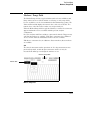
How to Roll Offscreen Data
How to Roll Offscreen Data
If there is offscreen data, it must be rolled back onscreen before it can be
viewed or acted upon. The types of data you typically find located offscreen
are Labels, Pods, Terms, Sequence Levels, and data listings. Each of the data
types have a roll field. These roll fields indicate offscreen data by becoming a
dark selectable field with small arrows showing the direction the data is
rolled. In addition, a roll indicator appears that indicates which rollable field
is currently active.
There are two ways to roll data. One is with the knob, the other is with the
Page keys. The following exercise demonstrates both ways by first having
you assign enough data to create offscreen data, then rolling the data.
Using the Knob
1 Press the analyzer Config MENU key.
2 Press the arrow keys to move the cursor to the A3/A4 pod pair field in
the Unassigned Pods list, then press the Select key.
3 Press the Up/Down arrow keys or rotate the knob to move the cursor to
the custom name for Analyzer 1 as shown below, then press the Select
key.
You should now have pod pairs A1/A2 and A3/A4 assigned to Analyzer 1.
Analyzer 1
Configuration menu
3–23
Using the Front-Panel Interface
How to Roll Offscreen Data
4 Press the analyzer Format MENU key.
5 Notice the roll indicator in the Pods roll field as shown. Rotate the
knob and notice how pods A1 through A4 are rolled left and right.
Pods roll field with roll
indicator
Labels roll field
Pods and Labels Roll Field
6 Press the Down arrow key to move the cursor to the Labels roll field
directly below the Pods roll field, then press the Select key or just
turn the knob.
7 Notice the roll indicator now switches to the Labels roll field. Rotate
the knob and notice how the column of labels roll up and down.
Using the Page Keys
8 Press the Up/Down Page keys and notice how the column of labels page
up and down.
9 Press the Up arrow key to move the cursor back to the Pods roll field,
then press the Select key.
10 Press the blue shift key, then press a Page key.
The left and right page keys must be preceded by the blue shift key each
time. Repeat this two key sequence to page the Pods left and right.
3–24
Using the Front-Panel Interface
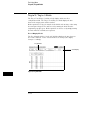
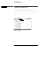
How to Use Assignment/Specification Menus
How to Use Assignment/Specification Menus
There are a number of assignment fields which you must assign or specify
what you want the instrument to do. Menus of this type are as follows:
• Assigning pod channels and clock channels to labels.
• Specifying patterns.
• Specifying edges.
Assigning Pod and Clock Channels
The channel assignment fields in both state and timing analyzers appear in
the Format menus and work identically. It should be noted that if you don’t
see any channel assignment fields, it merely means you do not have any pods
assigned to this analyzer or any labels turned on. The convention for channel
assignments is as follows:
* (asterisk) indicates assigned channels
. (period) indicates un-assigned channels
To assign channels to an analyzer, do the following exercise:
1 Press the analyzer Format MENU key.
2 Press the arrow keys to move the cursor to the channel assignment
field as shown below, then press the Select key.
Channel assignment
Channel Assignment Field
3–25
Using the Front-Panel Interface
How to Use Assignment/Specification Menus
When the channel assignment field is selected, an assignment pop-up
appears showing you the bit or channel to be assigned, and the two choices
directly above it.
Assignment choices
Assignment pop-up
Channel Assignment Pop-up
3 Turn all channels on (assign an asterisk) by either pressing the Select
key or by pressing the Up arrow key.
Individual bits or channels are highlighted by moving the cursor side to side
with the left/right arrow keys or by rotating the knob. The Select key toggles
the current choice. The up arrow assigns a channel, and the down arrow
unassigns a channel. In addition, the entire bank of channels are assigned or
cleared by pressing the Clear entry key.
4 When you are finished assigning channels, press the Done key.
3–26
Using the Front-Panel Interface
How to Use Assignment/Specification Menus
Specifying Patterns
Certain assignment fields require bit patterns to be specified. Patterns can
be specified in any one of the available number bases, except ASCII. A
pattern can contain a value or a "Don’t care."
The convention for "Don’t cares" in these menus is an "X" except in the
decimal base. If the base is set to decimal after a "don’t care" is specified, a $
character is displayed.
To specify a pattern, perform the following exercise:
1 Press the analyzer Trigger MENU key.
2 Press the arrow keys to move the cursor to the assignment field for
the "a" resource term as shown.
Resource term "a"
assignment field
Resource Term Assignment Field
3 Using the Hexadecimal keypad, enter a pattern, then press the Select
key.
In addition to using the numeric keypad, you can enter "Don’t cares" into the
entire assignment field by pressing the Clear entry key.
3–27
Using the Front-Panel Interface
How to Use Assignment/Specification Menus
Specifying Edges
Certain assignment fields require edge assignments to be specified. An edge
can be specified in any one of the available number bases.
You can select positive-going ( ↑ ), negative-going ( ↓ ), either edge ( ↕ ) or
no edge ( . ).
To specify an edge, perform the following exercise:
1 Press the analyzer Trigger MENU key.
2 Press the arrow keys to move the cursor to the Edge 1 assignment
field as shown, then press the Select key.
Edge assignment
field
Edge and Glitch Assignment Field
3–28
Using the Front-Panel Interface
How to Use Assignment/Specification Menus
When the Edge and Glitch assignment field is selected, an assignment pop-up
appears showing you the bit or channel to be assigned, and the five choices
directly above it.
Edge and glitch
selection list
Edge and Glitch Selection List
3 Press the Up/Down arrow keys to move the cursor to the desired edge
assignment, then press the left/right arrow key or turn the knob to move
the cursor to the next channel. Repeat step 3 until all of the desired
channels are assigned.
4 To close the assignment field, press the Done key.
Individual bits or channels are cleared by pressing the front-panel (.) period
key. The entire bank of channels are cleared by pressing the Clear entry key.
It should be noted that when you close the pop-up after specifying edges, you
see dollar signs ($ $ ... ) in the assignment field. This simply indicates the
logic analyzer can’t display the assignment correctly in the current number
base selected.
3–29
3–30
4
Using the Mouse and the
Optional Keyboard
The Mouse and the Optional Keyboard
This chapter explains how to use the mouse and the optional
keyboard interface (Agilent Technologies E2427A Keyboard Kit). The
keyboard and mouse can be used interchangeably with the knob and
front-panel keypad for all menu applications. The keyboard and
mouse functions fall into the two basic categories of cursor movement
and data entry.
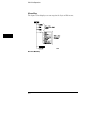
Both the keyboard or mouse can be connected to the keyboard/mouse
connector on the rear panel of the logic analyzer. If both are
connected at the same time, the keyboard is connected to the
analyzer and the mouse is connected to the keyboard.
When the keyboard and/or mouse is connected, a graphic is included
in the RS-232 / GPIB (or Printer/Controller) menu to represent the
interface options being used.
See Also
The documentation that comes with each interface device for complete
details on connecting them to each other or, to the logic analyzer.
4–2
Using the Mouse and the Optional Keyboard
Moving the Cursor
Moving the Cursor
The keyboard cursor is the location on the screen highlighted in inverse
video. To move the cursor, follow one of the methods described below.
Keyboard Cursor Movement
There are four cursor keys marked with arrows on the keyboard. These keys
perform the following movements:
•
•
•
•
Up-pointing arrow moves the cursor up.
Down-pointing arrow moves the cursor down.
Right-pointing arrow moves the cursor to the right.
Left-pointing arrow moves the cursor to the left.
The cursor keys do not wrap. This means that pressing the right-pointing
arrow when the cursor is already at the rightmost point in a menu will have
no effect. The cursor keys do repeat, so holding the key down is the fastest
way to continue keyboard cursor movement in a given direction.
Home Key (or corner arrow) If you want to move the cursor to the
first item in a menu, press the Home key. If you want to move the cursor
to the last item in a menu, press the Home and Shift keys simultaneously.
Next and Previous Keys The Next and Previous keys are used for
paging through listings. The Next key will display the next page of data,
if one exists. The Previous key will display the previous page of data, if
one exists.
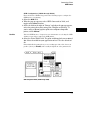
Selecting a Menu Item
To select a menu item using the optional keyboard, position the cursor (the
location highlighted in inverse video) on the desired menu item using one of
the methods described in the section “Moving the Cursor” and press either
the Return or the Select key.
4–3
Using the Mouse and the Optional Keyboard
Entering Data into a Menu
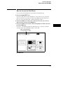
Mouse Cursor Movement
The mouse pointer (+) is positioned around the screen by moving the mouse
about on top of a desktop or other even surface.
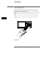
Selecting a Menu Item To select a menu field, simply move the
pointer on top of the desired field and press the upper-left button.
To duplicate the front-panel knob, hold down the upper-right button while
moving the mouse around the desktop. Moving the mouse up or to the right
duplicates turning the knob clockwise. Moving the mouse down or to the left
duplicates turning the knob counterclockwise.
Entering Data into a Menu
Keyboard Data Entry
When an assignment field is selected, the cursor is displayed under the
leftmost digit in the particular field. When you type in a number or letter, it is
displayed in the cursor position, and the cursor is advanced. Cursor keys
move the cursor within the assignment field. Pressing either the Return key
or the Enter key will terminate data entry for that item.
If you want to erase the data entry, press the Clear Line key, the Clear
Display key, or the Delete Line key.
Mouse Data Entry
When an assignment field is selected, a pop-up keypad or assignment menu
appears. Use the pop-up menus to assign letters, numbers, symbols, or unit
of measure. When the Done field is selected, the pop-up closes and the
selected values are entered into the assignment field.
4–4
Using the Mouse and the Optional Keyboard
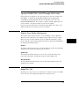
Using the Keyboard Overlays
Using the Keyboard Overlays
Two keyboard overlays are included in the E2427A Keyboard Kit. The
overlays shown below redefine functions of the function keys and the
numeric keypad.
Function Key Overlay
Key
Function Performed
F1
Selects System subset menus
F2
Selects the Analyzer Configuration Menu (ignore Scope Channel Menu)
F3
Selects the Analyzer Format Menu (ignore Scope Display Menu)
F4
Selects the Analyzer Trigger Menu (ignore Scope Trigger Menu)
F5
Selects the Analyzer Listing Menu (ignore Scope Marker Menu)
F6
Selects the Analyzer Waveform Menu (ignore Scope Auto-Measure Menu)
F7
Selects the Print All function
F8
Selects the Run Repetitive function
4–5
Using the Mouse and the Optional Keyboard
Using the Keyboard Overlays
Numeric Keypad Overlay
4–6
Key
Function Performed
Tab
Don’t care "X"
Enter
Done
Stop (unlabeled)
Stop
Using the Mouse and the Optional Keyboard
Defining Units of Measure
Defining Units of Measure
In addition to the function keys, other keys on the keyboard invoke the unit
of measure selections.
Time Units
Key
Time Units
S
Selects the seconds units
M
Selects the milliseconds units
U
Selects the microseconds units
N
Selects the nanoseconds units
Voltage Units
Key
Voltage Units
V
Selects volts
M
Selects millivolts
4–7
Using the Mouse and the Optional Keyboard
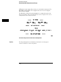
Assigning Edge Triggers
Assigning Edge Triggers
Several keys invoke edge assignments.
Key
Edge Trigger Assignment
U
Selects the up or rising edge.
D
Selects the down or falling edge.
R
Selects the rising edge.
F
Selects the falling edge.
B
Selects either the rising or falling edge.
∗ (asterisk)
Assigns a glitch.
. (period)
Assigns a Don’t Care
Closing a Menu
To exit a menu, press either the Done or Enter key. The Enter key is
mapped to the Done key, so pressing either key closes the menu.
4–8
5
Connecting a Printer
Connecting a Printer
The logic analyzer can output its screen display to various GPIB,
RS-232C, and Centronix graphics printers (1664A only). Configured
menus as well as waveforms, listings and other data, can be printed
for complete measurement documentation.
5–2
Connecting a Printer
GPIB Printers
GPIB Printers
The logic analyzer interfaces directly with HP PCL printers supporting the
printer command language or with Epson printers supporting the Epson
standard command set. These printers must also support GPIB and Listen
Always. Printers currently available from Hewlett-Packard with these
features include:
•
•
•
•
•
HP ThinkJet
HP LaserJet
HP PaintJet
HP DeskJet
HP QuietJet
It should be noted that an GPIB printer must always be in Listen mode, and
the analyzer’s GPIB port does not respond to service requests (SRQ) when
controlling a printer. The SRQ enable setting for the GPIB printer has no
effect on 16600B printer operation.
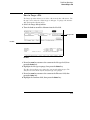
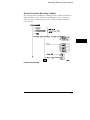
GPIB Printer Setup
To set up the GPIB printer, perform the following steps:
1 Turn off the instrument and connect an GPIB cable from the printer
to the GPIB connector on the rear panel of the instrument. Turn on
the instrument.
GPIB Connector
(location different
for 1664A)
GPIB Connector
5–3
Connecting a Printer
GPIB Printers
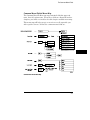
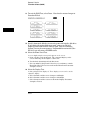
2 Make sure the printer is in Listen Always (or Listen Only). For
example, the figure below shows the GPIB configuration switches for
an GPIB ThinkJet printer. For the Listen Always mode, move the
second switch from the left to the “1" position.
Since the instrument doesn’t respond to SRQ EN (Service Request Enable),
the position of the first switch doesn’t matter.
Listen Always Switch Setting
5–4
Connecting a Printer
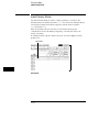
GPIB Printers
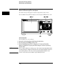
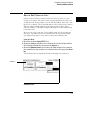
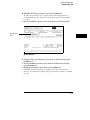
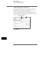
GPIB Configuration (1660A through 1663A)
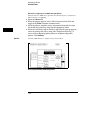
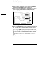
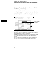
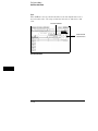
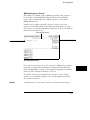
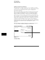
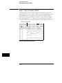
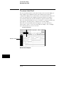
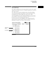
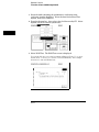
From the RS-232 / GPIB menu, perform the following steps to configure the
GPIB interface for printing:
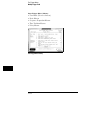
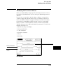
1 Select the GPIB field.
2 When the pop-up appears, select "GPIB Connected to" field, and
toggle to the Printer selection.
3 Select the field to the right of “Printer” and when the pop-up appears,
select the printer that you’re using (like, ThinkJet or QuietJet). If
you’re using an Epson graphics printer or an Epson-compatible
printer, select Alternate.
See Also
"RS-232 / GPIB Interface" chapter for more information on selecting the GPIB
Address to match the setup for the GPIB printer.
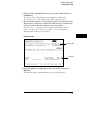
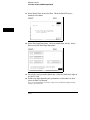
4 Select the "Print Width" field. The print width toggles between 80 and
132. Select the width for your application or leave it at the default of
80.
Print width tells the printer that you are sending up to 80 or 132 characters
per line (when you Print All) and is totally independent of the printer itself.
GPIB Configuration Menu (1660A through 1663A)
5–5
Connecting a Printer
GPIB Printers
If you select 132 characters per line when using other than the QuietJet
selection, the listings are printed in a compressed mode. Compressed mode
uses smaller characters to allow the printer to print more characters within a
given area.
If you select 132 characters per line for the QuietJet selection it can print a
full 132 characters per line without going to compressed mode, but the
printer must have wider paper.
If you select 80 characters per line for any printer, a maximum of 80
characters are printed per line.
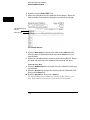
5 Select the "Print Length" field. The print length toggles between 11
and 12. Select the length for your application or leave it at the default
of 11.
Print length tells the printer the page length for the type of paper you are
using.
6 Press the front-panel Done key.
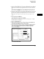
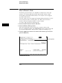
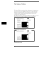
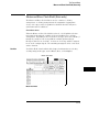
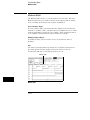
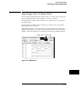
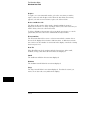
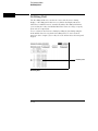
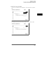
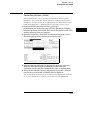
Optional GPIB Configuration (1664A)
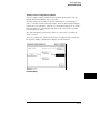
From the Printer/Controller menu, perform the following steps to configure
the GPIB interface for printing:
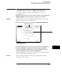
1 Select the Printer Setup field.
2 When the pop-up appears, select "Printer Connected to GPIB" field,
and toggle to the Printer selection.
3 Select the field to the right of “Printer” and when the pop-up appears,
select the printer that you’re using (like, ThinkJet or QuietJet). If
you’re using an Epson graphics printer or an Epson-compatible
printer, select Alternate.
See Also
"RS-232 / GPIB Interface" chapter for more information on selecting the GPIB
Address to match the setup for the GPIB printer.
4 Select the "Print Width" field. The print width toggles between 80 and
132. Select the width for your application or leave it at the default of
80.
Print width tells the printer that you are sending up to 80 or 132 characters
per line (when you Print All) and is totally independent of the printer itself.
If you select 132 characters per line when using other than the QuietJet
selection, the listings are printed in a compressed mode. Compressed mode
uses smaller characters to allow the printer to print more characters within a
given area.
5–6
Connecting a Printer
GPIB Printers
GPIB Configuration Menu (1664A)
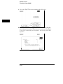
If you select 132 characters per line for the QuietJet selection it can print a
full 132 characters per line without going to compressed mode, but the
printer must have wider paper.
If you select 80 characters per line for any printer, a maximum of 80
characters are printed per line.
5–7
Connecting a Printer
RS-232C Printers
RS-232C Printers
The instrument interfaces directly with RS-232C printers including the HP
ThinkJet, HP QuietJet, HP LaserJet, HP PaintJet, and HP DeskJet printers.
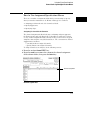
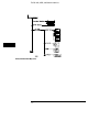
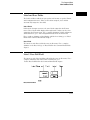
RS-232C Printer Setup
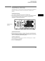
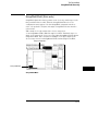
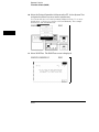
To set up the RS-232C printer, perform the following steps:
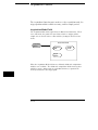
1 Turn off the instrument and connect an RS-232C cable from the
printer to the RS-232C connector on the rear panel of the instrument.
Turn on the instrument.
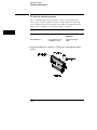
RS-232C connector
(location different
on 1664A)
RS-232C Connector
5–8
Connecting a Printer
RS-232C Printers
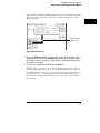
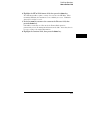
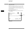
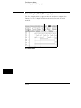
2 Before turning on the printer, locate the mode configuration switches
on the printer and configure them as follows:
• The HP QuietJet series printers have two banks of mode function switches
inside the front cover. Push all the switches down to the “0" position as
shown.
• For the HP 2225D (RS-232 HP ThinkJet) printer, the mode switches are
on the rear panel of the printer. Push all the switches down to the “0"
position as shown .
• For the HP LaserJet printer, the switch settings can remain in the factory
default settings.
5–9
Connecting a Printer
RS-232C Printers
RS-232C Configuration (1660A through 1663A)
From the RS-232 / GPIB menu, perform the following steps to configure the
RS-232 interface for printing:
1 Select the RS-232 field.
2 When the pop-up appears, select "RS-232 Connected to" field, and
toggle to the Printer selection as shown below.
3 Set the baud rate, stop bits, parity, and protocol to match the setup
for the RS-232C printer by selecting the appropriate fields.
4 Select the field to the right of “Printer” and when the pop-up appears,
select the printer that you’re using (like, ThinkJet or QuietJet). If
you’re using an Epson graphics printer or an Epson-compatible
printer, select Alternate.
See Also
"RS-232 / GPIB Interface" chapter for more information.
RS-232 Configuration Menu (1660A through 1663A)
5–10
Connecting a Printer
RS-232C Printers
5 Select the "Print Width" field. The print width toggles between 80 and
132. Select the width for your application or leave it at the default of
80.
Print width tells the printer that you are sending up to 80 or 132 characters
per line (when you Print All) and is totally independent of the printer itself.
6 Touch the" Print Length" field and print length toggles between 11 and
12. Select the length for your application or leave it at the default of
11.
Print length tells the printer the page length for the type of paper you are
using.
7 Press the front-panel Done key.
Optional RS-232C Configuration (1664A)
From the Printer/Controller menu, perform the following steps to configure
the RS-232 interface for printing:
1 Select the Printer Setup field.
2 When the pop-up appears, select "Printer Connected to RS-232" field,
and toggle to the Printer selection as shown below.
3 Select the field to the right of “Printer” and when the pop-up appears,
select the printer that you’re using (like, ThinkJet or QuietJet). If
you’re using an Epson graphics printer or an Epson-compatible
printer, select Alternate.
RS-232 Configuration Menu (1664A)
5–11
Connecting a Printer
RS-232C Printers
See Also
"RS-232 / GPIB Interface" chapter for more information on selecting the baud
rate, stop bits, parity, and protocol to match the setup for the RS-232C
printer.
4 Select the "Print Width" field. The print width toggles between 80 and
132. Select the width for your application or leave it at the default of
80.
Print width tells the printer that you are sending up to 80 or 132 characters
per line (when you Print All) and is totally independent of the printer itself.
5 Touch the" Print Length" field and print length toggles between 11 and
12. Select the length for your application or leave it at the default of
11.
Print length tells the printer the page length for the type of paper you are
using.
6 Press the front-panel Done key.
5–12
Connecting a Printer
Parallel Printers (1664A Only)
Parallel Printers (1664A Only)
The 1664A interfaces directly with Centronix (parallel) printers including the
HP ThinkJet, HP QuietJet, HP LaserJet, HP PaintJet, and HP DeskJet
printers.
Parallel Printer Setup
To set up the parallel printer, perform the following steps:
1 Turn off the instrument and connect a parallel cable from the printer
to the parallel printer port connector on the rear panel of the
instrument. Turn on the instrument.
Parallel Printer Port
connector
Parallel Printer Port Connector
2 Before turning on the printer, configure the printer (switches/menu)
for parallel operation. Information for parallel operation is located in
the User’s Guide provided with the printer.
Parallel Configuration
From the Printer/Controller menu, perform the following steps to configure
the Parallel interface for printing:
1 Select the Printer Setup field.
5–13
Connecting a Printer
Parallel Printers (1664A Only)
2 When the pop-up appears, select "Printer Connected to Parallel Port"
field, and toggle to the Printer selection as shown below.
3 Select the field to the right of “Printer” and when the pop-up appears,
select the printer that you’re using (like, ThinkJet or QuietJet). If
you’re using an Epson graphics printer or an Epson-compatible
printer, select Alternate.
Parallel Port Configuration Menu
4 Select the "Print Width" field. The print width toggles between 80 and
132. Select the width for your application or leave it at the default of
80.
Print width tells the printer that you are sending up to 80 or 132 characters
per line (when you Print All) and is totally independent of the printer itself.
5 Touch the" Print Length" field and print length toggles between 11 and
12. Select the length for your application or leave it at the default of
11.
Print length tells the printer the page length for the type of paper you are
using.
6 Press the front-panel Done key.
5–14
Connecting a Printer
Connecting to Other Hewlett-Packard Printers
Connecting to Other Hewlett-Packard Printers
The instrument can also be used with other Hewlett-Packard graphics
printers. Simply connect the printer to the instrument using the appropriate
cable (GPIB, RS-232C, or Centronix) and configure the instrument as shown
below.
For this HP Printer
Select this Printer
from the pop-up
HP 2631G
QuietJet
HP 2671G
ThinkJet
HP 2673A
ThinkJet
HP 9876A
ThinkJet
HP 2932/34 (option 046)
QuietJet
HP Printer Configuration Guide
5–15
Connecting a Printer
Connecting to Other Hewlett-Packard Printers
GPIB printers must support Listen Always to work with the instrument. The
HP 82906A graphics printer is not supported because it does not support
Listen Always on GPIB.
The HP 2932A or HP 2934A option 046 printer is configured from the front
panel of the printer, instead of with switches on the rear panel. The correct
configuration for the analyzer is shown.
Front Panel Configuration for the HP 2932A or 2934A Option 046
See Also
The Programming Reference Manual for information on setting up an
external controller to activate the printer.
5–16
Connecting a Printer
Printing the Display
Printing the Display
After connecting the printer to the instrument and setting the printer and
instrument configurations, apply power to the printer.
Each menu has a Print field in the upper-right corner. Select the Print field
and a pop-up appears, displaying your choices.
• Cancel is used to stop the instrument from sending data.
• Print Screen prints everything shown on the screen.
• Print All (available only in certain menus) prints all of the information
listed for that display, including any listings that do not appear on screen.
These listings can be 80 or 132 characters wide, depending on the Print
Width setting.
• Print Disk is used to print measurement data to a DOS or LIF disk, which
can then be copied into a computer file. The Print Disk function is the
same as the Print All function except the data is printed to a disk.
To initiate a hard copy print, perform the following steps:
1 Using the arrow keys highlight the Print field, then press the Select key.
2 Select the Print Screen or Print All field, then press the Select key.
The instrument does not check the operation of the printer, so no error
messages are displayed.
See Also
"Print field" in the Common Menu Fields chapter for more information on
Print Disk.
5–17
5–18
6
Disk Drive Operations
Disk Drive Operations
The logic analyzer has a built in 3.5 inch, double-sided, high-density or
double-density, flexible disk drive. The disk drive is compatible with
both LIF (Logical Interchange Format) and DOS (Disk Operating
System) formats.
This chapter describes the disk operations available in the logic
analyzer and how to use them. It is organized into separate "How to"
examples demonstrating the use of the Disk menu and all the disk
operations.
The Disk Operations
Nine disk operations are available:
• Autoload
Designates a set of configuration files to be loaded automatically the
next time the analyzer is turned on.
• Copy
Any file can be copied from one disk to another, from one directory to
another, or to the same disk.
• Duplicate Disk
All volume labels, directories, and file positions from one disk are
copied exactly to another disk. The new disk is formatted to match
the source disk if it is required. All files on the destination disk will be
destroyed with this operation.
• Format Disk
Any double-sided, double-density, 3.5-inch flexible disk can be
formatted in either LIF or DOS format. The directory and all files on
the disk will be destroyed with this operation.
6–2
Disk Drive Operations
• Load
Instrument system configurations, analyzer measurement setups,
including measurement data, and inverse assembler files for the
analyzer can be loaded from the disk drive.
• Make Directory
This function creates a new directory on a DOS disk. Files can me
saved or copied to the new directory isong the store and copy
commands.
• Pack Disk
This function packs files on a LIF disk. Packing removes all empty or
unused sectors between files on a disk so that more space is available
for files at the end of the disk.
• Purge
Any file on a disk can be purged (deleted) from the disk.
• Rename
Any filename on a disk can be changed to another name.
• Store
Instrument system configurations and analyzer measurement setups
including measurement data can be stored to the disk drive.
Disk Operation Safeguards
If there is a problem or additional information is needed to execute an
operation, a pop-up appears near the center of the screen displaying
the status of the operation (for example, it displays an error message
or prompts you to swap disk).
If executing a disk operation could destroy or damage a file, a pop-up
appears when you select Execute. If you don’t want to complete the
operation, select Cancel to cancel the operation. Otherwise, select
Continue and the operation will be continued.
6–3
Disk Drive Operations
Menu Map
The figure below displays a menu map for the System Disk menu.
Disk Drive Menu Map
6–4
Disk Drive Operations
How to Access the Disk Menu
How to Access the Disk Menu
To access the System Disk menu, perform the following steps:
1 Press the System MENU key.
If you have just turned on the instrument, or if you have not accessed any
System menus since powerup, the first menu displayed is the Disk menu.
If you are not in the Disk menu, continue with steps 2 and 3.
2 Press the arrow keys to move the cursor to the menu name field as
shown below, then press the Select key.
3 Press the arrow keys or turn the knob to highlight the Disk field, then
press the Select key.
If you have a disk installed when the Disk menu is accessed, the analyzer
automatically reads and displays all files on the disk.
Menu name field (displays
Printer/Controller on 1664A)
Menu Name Field
6–5
Disk Drive Operations
How to Install a Disk
How to Install a Disk
To install a flexible disk into the disk drive, perform the following steps:
1 Hold the disk so the disk label is on top and the metal auto-shutter is
away from you. See the figure below.
2 Push the disk gently, but firmly, into the disk drive until it clicks into
place.
You can use double-sided, double-density and double-sided, high-density
disks.
To display all files on any disk, insert the disk into the drive, then turn the
knob.
Installing a Disk
6–6
Disk Drive Operations
How to Select a Disk Operation
How to Select a Disk Operation
Although some default values are provided for disk operations, a disk
operation may require additional information from the user. This information
is entered in the appropriate fields within each disk operation.
To select a disk operation, perform the following steps:
1 Press the arrow keys to highlight the disk operation field shown in the
figure below. Then press the Select key.
Disk operation field
Disk Operation Field
2 Turn the knob to highlight the desired disk operation field, then press
the Done or Select key.
6–7
Disk Drive Operations
How to Load a File
How to Load a File
The Load operation allows you to load prestored configuration files. Use this
operation when you want to quickly restore the analyzer to a configuration
used in a previous measurement or condition.
When configurations are stored to the disk, you are given the option to store
System only, Analyzer only, or All (System and Analyzer). So, when you load
a file into the analyzer, you are given the same options.
To load a file from the disk, perform the following steps:
1 Insert the source disk into the disk drive.
2 Select the Load disk operation.
When the Load selection is made, the analyzer reads the disk directory and
displays a list of all files on the disk.
3 Press the arrow keys to move the cursor to the file type field shown
below, then press the Select key.
File type field
File Type Parameter Field
6–8
Disk Drive Operations
How to Load a File
4 Turn the knob to highlight the file type you want to load, then press
the Select key.
The System choice loads things like Bus and display configurations.
The Analyzer choice loads analyzer menus and measurement data.
5 Turn the knob and notice the changing filenames in the filename field
shown below, and how the cursor bar scrolls the list of available files.
Using the knob, scroll to the filename you want to load.
The two spaces(_ _) after the filename designates that this file is for the
system. One space and a letter (for example, "_A") after the filename
designates that the file is for the analyzer.
Filename Selection
Filename field
Scroll bar
6 Press the arrow keys to highlight the Execute field, then press the
Select key.
The disk drive indicator light illuminates as the file is being loaded.
6–9
Disk Drive Operations
How to Format a Disk
How to Format a Disk
The Format operation allows you to initialize new disks for use in the logic
analyzer. The analyzer will format double-sided, double density or high
density disks in both LIF and DOS formats. The analyzer does not support
any single-sided formats.
The logic analyzer does not support track sparing during formatting. If a bad
track is found, the disk is considered bad. If a disk has been formatted
elsewhere with track sparing, it will be read successfully.
To format a disk, perform the following steps:
1 Insert the disk to format into the disk drive.
2 Select the Format Disk operation.
When the Format Disk selection is made, the analyzer reads the disk
directory and displays all files. The DISK ERROR message appears if the disk
is a new un-formatted disk. This is normal, continue the format process.
3 Press the arrow keys to move the cursor to the format type field, then
press the Select key.
Format type field
LIF or DOS Format Selection
6–10
Disk Drive Operations
How to Format a Disk
4 Highlight the LIF or DOS format field, then press the Select key.
The instrument will recognize a variety of sector sizes for LIF disks. When
formatting LIF disks, the instrument creates 1024 byte sectors. DOS disks
always have 512 byte sectors.
5 Press the arrow keys to move the cursor to the Execute field, then
press the Select key.
It should be noted that once Executed, the Format Disk operation
permanently erases all existing information from the disk. After that, there is
no way to retrieve the original information.
6 Highlight the Continue field, then press the Select key.
6–11
Disk Drive Operations
How to Store Files on a Disk
How to Store Files on a Disk
The Store operation allows you to store instrument configurations and
measurement data. Use this operation when you want to save the present
analyzer setup to recall at a later time.
When configurations are stored to the disk, you are given the option to store
System only, Analyzer only, or All (System and Analyzer).
To store a file, perform the following steps:
1 Insert the destination disk into the disk drive.
2 Select the Store disk operation.
When the Store selection is made, the instrument reads the disk directory
and displays a list of all files on the disk. If there are no files, NO FILES is
displayed.
3 Press the arrow keys to move the cursor to the file type field, then
press the Select key.
File type field
File Type Parameter Field
6–12
Disk Drive Operations
How to Store Files on a Disk
4 Turn the knob to highlight the file type you want to store, then press
the Select key.
The System choice stores things like Bus and display configurations.
The Analyzer choice stores analyzer menus and measurement data.
The All choice stores System and Analyzer types.
5 Press the arrow keys to move the cursor to the file name field.
File name field
File Name Field
6 Using the front-panel keypad, type in a filename to assign to the new
file, then press the Select key.
The filename must start with a letter and may contain up to eight characters.
It can be any combination of letters and numbers, but there can be no blank
spaces between any of the characters.
If you want to select an existing filename, simply turn the knob to scroll
existing filenames through the field. Also, notice how the cursor bar
highlights the same name in the list of filenames.
The two spaces(_ _) after the filename designates that this file is for the
system. One space and a letter (for example, "_A") after the filename
designates that the file is for the analyzer.
6–13
Disk Drive Operations
How to Store Files on a Disk
7 Press the arrow keys to move the cursor to the file description field.
File description
File Description Field
8 Using the front-panel keypad, type in a description of the file, then
press the Select key.
A file description can contain up to 32 characters, but also can be left blank.
This field is for your convenience to make it easier to identify the type of data
in each file.
9 Press the arrow keys to move the cursor to the Execute field, then
press the Select key.
10 Highlight the Continue field, then press the Select key.
6–14
Disk Drive Operations
How to Rename a File
How to Rename a File
The Rename operation allows you to give a new name to a previously stored
file. The only restriction is that you cannot rename a file to an already
existing filename.
To rename a file, perform the following steps:
1 Select the Rename disk operation.
2 Turn the knob until the filename you want to rename is scrolled into
the file field.
File field
Type field
File Field
3 Press the arrow keys to move the cursor to the type field, then press
the Select key.
4 Turn the knob to highlight the file type you want to rename, then
press the Select key.
The All selection allows you to rename all of the system and analyzer types.
The analyzer selection allows only the analyzer type to be renamed.
6–15
Disk Drive Operations
How to Rename a File
5 Press the arrow keys to move the cursor to the new filename field.
New filename
field
New Filename Field
6 Using the front-panel keypad, type in the new filename , then press
the Select key.
7 Press the arrow keys to move the cursor to the Execute field, then
press the Select key.
6–16
Disk Drive Operations
How to Autoload a File
How to Autoload a File
The Autoload operation allows you to designate a set of configuration files to
be loaded automatically the next time the instrument is turned on. This
allows you to change the default configuration of certain menus to a
configuration that better fits your needs.
To enable the Autoload operation, perform the following steps:
1 Select the Autoload disk operation.
2 Press the arrow keys to move the cursor to the Enable/Disable
selection field, then press the Select key.
3 Highlight the Enable field, then press the Select key.
4 Press the arrow keys to move the cursor to the autoload filename field.
Enable/Disable field
Autoload filename
field
Autoload Filename Parameter Field
6–17
Disk Drive Operations
How to Autoload a File
5 Turn the knob until the filename you want to autoload is scrolled into
the filename parameter field.
6 Press the arrow keys to move the cursor to the Execute field, then
press the Select key.
An autoload file is created and placed at the top of the list of files. The file
description contains the filename to be autoloaded and indicates whether or
not the Autoload operation is enabled.
Filename
parameter field
Autoload Filename Field
It should be noted that Autoload loads all of the files for a given filename. If
you want to load only the file for a type, rename that file to separate it from
the other files and enable it as the current Autoload file.
As long as Autoload is enabled before the instrument is shut off, Autoload will
remain enabled when you powerup the instrument and load the configuration
files.
6–18
Disk Drive Operations
How to Purge a File
How to Purge a File
The Purge operation allows you to delete a file from the list of filenames. The
file type can be either the analyzer type or All types. To purge a file from the
disk, perform the following steps:
1 Select the Purge disk operation.
2 Turn the knob to scroll the filename into the file field.
File type field
File field
File Field
3 Press the arrow keys to move the cursor to the file type field, then
press the Select key.
4 Highlight the file type to purge, then press the Select key.
The All selection allows you to purge the system and analyzer types. The
analyzer selection allows only the analyzer type to be purged.
5 Press the arrow keys to move the cursor to the Execute field, then
press the Select key.
6 Highlight the Continue field, then press the Select key.
6–19
Disk Drive Operations
How to Copy a File
How to Copy a File
The Copy operation allows you to make a duplicate copy of an existing file on
the same disk or a different disk. If you copy the file to the same disk, the
only restriction is that you must give the copied file a new name. You can
specify to copy All types or just the analyzer part of a file.
To make copies of a file, perform the following steps:
1 Select the Copy disk operation.
2 Turn the knob until the filename you want to copy is scrolled into the
file field.
File field
Type field
Copy Filename Parameter Field
3 Press the arrow keys to move the cursor to the type field, then press
the Select key.
6–20
Disk Drive Operations
How to Copy a File
4 Highlight the file type to copy, then press the Select key.
The All selection allows you to copy the system and analyzer parts of a
configuation file set. The analyzer selection allows only the analyzer part to
be copied.
5 Press the arrow keys to move the cursor to the new filename field.
New filename
field
New filename Field
6 Using the front-panel keypad, type in the new filename, then press
the Select key.
7 Press the arrow keys to move the cursor to the Execute field, then
press the Select key.
8 Highlight the Continue field, then press the Select key.
It is highly recommended that you complete the Copy operation in its
entirety. Selecting Cancel during a Copy operation may result in a corrupted
file copy.
6–21
Disk Drive Operations
How to Pack a Disk
How to Pack a Disk
By purging files from the disk and adding other files, you may end up with
blank areas on the disk (between files) that are too small for the new files
you are creating. On LIF disks, the Pack Disk operation packs the current
files together, removing unused areas from between the files so that more
space is available for files at the end of the disk. On DOS disks, the Pack Disk
operation is not displayed.
To pack the disk, perform the following steps:
1 Select the Pack Disk operation.
2 Press the arrow keys to move the cursor to the Execute field, then
press the Select key.
Execute field
Pack Disk Operation
6–22
Disk Drive Operations
How to Duplicate a Disk
How to Duplicate a Disk
The Duplicate Disk operation copies the volume labels and directories from
one disk to another. If necessary, the new disk is formatted to match the
source disk. This operation allows you to make a back-up copy of your
important disks so you won’t lose important data in the event that a disk
wears out, is damaged, or a file is accidently deleted.
To duplicate the disk, perform the following steps:
1 Select the Duplicate Disk operation.
2 Press the arrow keys to move the cursor to the Execute field, then
press the Select key.
Execute field
The Duplicate Disk Operation
6–23
Disk Drive Operations
How to Duplicate a Disk
3 Highlight the Continue field, then press the Select key.
When “Insert DESTINATION disk” appears, insert the destination disk into
the disk drive, and when "Insert SOURCE disk” appears, remove the
destination disk and reinstall the source disk. The number of times you need
to change the disks depends on whether you have a double-density or
high-density disk. Simply follow the instructions and select Continue to
continue.
It should be noted that the original directory and files on the destination disk
are destroyed by the Duplicate Disk operation.
6–24
Disk Drive Operations
How to Make a Directory
How to Make a Directory
The Make a Directory operation is used to create a new, blank directory or
sub-directory on a DOS disk. After a new directory is created, files can be
copied and stored using the COPY and STORE functions. Note that only the
selected directory’s contents are shown (the selected directory is displayed
in the lower left portion of the display). The Change Dir. selection is used to
change directories. On LIF disks, the Make a Directory operation is not
displayed.
To make a new directory on the DOS disk, perform the following steps:
1 Select the Make Directory operation.
2 Press the arrow keys to move the cursor to the New Directory Name
field, then press the Select key.
3 Using the front-panel keypad, type in the new directory name, then
press the Select key.
If you are currently in a directory, the Make a Directory selection will create a
sub-directory within the current directory.
4 Press the arrow keys to move the cursor to the Execute field, then
press the Select key.
new directory
name field
Execute field
Change Directory field
Current Directory
Make Directory Operation
6–25
Disk Drive Operations
How to Make a Directory
5 To select the new directory, or display the contents of a different
directory, press the arrow keys to move the cursor to the Change Dir.
field, then press the Select key until "PWD: \" is displayed. Use the
knob to choose the desired directory, then press the Select key to
display the contents of the selected disectory.
6–26
7
The RS-232C, GPIB, and
Centronix Interface
The RS-232C, GPIB, and Centronix
Interface
This chapter describes the controller and printer interfaces and their
configuration. It defines the GPIB interface and describes how to
select any one of the 31 different GPIB addresses available. It also
defines the RS-232C interface and tells you how to select a baud rate,
how to change the stop bits, how to set the parity and data bits, and
how to change the protocol. The 1664A Centronix (parallel) interface
(printer only) is also described.
GPIB
configuration
RS-232
configuration
RS-232 / GPIB Interface Menu (1660A through 1663A)
Controller
Printer
RS-232 / GPIB Interface Menu (1664A)
7–2
The RS-232C, GPIB, and Centronix Interface
RS-232 / GPIB Menu Map (1660A through 1663A)
The following menu map illustrates all fields and the available options
in the RS-232 / GPIB menu. The menu map will help you get an
overview as well as provide you with a quick reference of what the
RS-232 / GPIB menu contains.
RS-232 / GPIB Menu Map
7–3
The RS-232C, GPIB, and Centronix Interface
RS-232 / GPIB Menu Map (Cont).
7–4
The RS-232C, GPIB, and Centronix Interface
Printer/Controller Menu Map (1664A)
The following menu map illustrates all fields and the available options in the
Printer/Controller menu. The menu map will help you get an overview as
well as provide you with a quick reference of what the Printer/Controller
menu contains.
Printer/Controller Menu Map
7–5
The RS-232C, GPIB, and Centronix Interface
Printer/Controller Menu Map (Cont).
7–6
The RS-232C, GPIB, and Centronix Interface
The Controller Interface
The instrument is equipped with a standard RS-232C interface and an
GPIB interface that allow you to connect to a controller (GPIB and
RS-232C optional on the 1664A). Either interface gives you remote
access for running measurements, for up-loading and down-loading
configurations and data, and more.
The Printer Interface
The instrument can output its screen display to various GPIB,
RS-232C, and Centronix (1664A only) graphics printers. Configured
menus as well as waveforms and other data can be printed for
complete measurement documentation.
See Also
"Connecting a Printer" for more details.
Agilent Technologies 1660A Series Logic Analyzers Programming
Manual for more information on the controller interface.
7–7
The RS-232C, GPIB, and Centronix Interface
The GPIB Interface
The GPIB Interface
The General Purpose Interface Bus (GPIB) is Agilent Technologies’
implementation of IEEE Standard 488-1978, “Standard Digital Interface for
Programmable Instrumentation.” The GPIB is a carefully defined interface
that simplifies the integration of various instruments and computers into
systems.
The GPIB interface uses an addressing technique to ensure that each device
on the bus (interconnected by GPIB cables) receives only the data intended
for it. To accomplish this, each device is set to a different address and this
address is used to communicate with other devices on the bus.
Selecting an Address (1660A through 1663A)
The GPIB address can be set to 31 different GPIB addresses, from 0 to 30.
Simply choose a compatible address of your device and software.
To select an GPIB address perform the following steps:
1 From the RS-232 / GPIB menu, select the GPIB field.
2 Turn the front-panel knob to select the GPIB Address, then press the
Done key.
GPIB field
GPIB Configuration Pop-up Menu (1660A through 1663A)
7–8
The RS-232C, GPIB, and Centronix Interface
The GPIB Interface
Selecting an Address (1664A)
The GPIB address can be set to 31 different GPIB addresses, from 0 to 30.
Simply choose a compatible address of your device and software.
To select an GPIB address perform the following steps:
1 From the Printer/Controller menu, select the Communications field.
2 When the pop-up menu appears, select "GPIB Address" field, then
press the Select key.
3 Turn the front-panel knob to select the GPIB Address, then press the
Done key.
GPIB field
GPIB Configuration Pop-up Menu (1664A)
7–9
The RS-232C, GPIB, and Centronix Interface
The RS-232C Interface
The RS-232C Interface
The RS-232C interface is Agilent Technologies’ implementation of EIA
Recommended Standard RS-232C, “Interface Between Data Terminal
Equipment and Data Communications Equipment Employing Serial Binary
Data Interchange.”
With this interface, data is sent one bit at a time and characters are not
synchronized with preceding or subsequent data characters. Each character
is sent as a complete entity without relationship to other events.
RS-232C field
RS-232C Configuration Pop-up Menu (1660A through 1663A)
RS-232C field
RS-232C Configuration Pop-up Menu (1664A)
7–10
The RS-232C, GPIB, and Centronix Interface
The RS-232C Interface
Baud Rate
The baud rate is the rate at which bits are transferred between the interface
and the peripheral. The baud rate must be set to transmit and receive at the
same rate as the peripheral.
To set the baud rate, select the Baud Rate field. Then, select the desired rate
from the pop-up selection list.
Stop Bits
Stop Bits are used to identify the end of a character. The number of Stop
Bits must be the same for the controller as for the logic analyzer.
To change the Stop Bits, select the Stop Bits field, then select the desired
stop bit from the pop-up selection list.
Parity
The parity bit detects errors as incoming characters are received. If the
parity bit does not match the expected value, the character is assumed to be
incorrectly received. The action taken when an error is detected depends on
how the interface and the device program are configured.
Parity is determined by the requirements of the system. The parity bit may
be included or omitted from each character by enabling or disabling the
parity function.
To set the parity bit, select the Parity field, then select the desired Parity bit
from the pop-up selection list.
Data Bits
Data bits are the number of bits sent and received per character that
represent the binary code of that character. The 1660A Series supports the
8-bit binary code.
7–11
The RS-232C, GPIB, and Centronix Interface
The RS-232C Interface
Protocol
Protocol governs the flow of data between the instrument and the external
device.
To change the protocol, select the Protocol field, then select the desired the
desired option from the pop-up selection list
With less than a 5-wire interface, selecting None does not allow the sending
or receiving device to control how fast the data is being sent. No control over
the data flow increases the possibility of missing data or transferring
incomplete data.
With a full 5-wire interface, selecting None allows a hardware handshake to
occur. With a hardware handshake, hardware signals control data flow. The
13242G cable allows the logic analyzer to support hardware handshake.
Xon/Xoff Xon/Xoff stands for Transmit On/Transmit Off. With this
mode, the receiver controls the data flow and can request that the
printer stop data flow at any time.
7–12
The RS-232C, GPIB, and Centronix Interface
The Centronix Interface (1664A Only)
The Centronix Interface (1664A Only)
The Centronix interface is Agilent Technologies’ implementation of the
industry standard parallel printer interface. Note that the Centronix
interface can only be used as a printer interface, and is not intended for use
with a controller.
With this interface, 8-bits of data are sent in parallel (at the same time) to the
printer, with seven additional lines used for handshaking, status, and timing.
See Also
"Connecting a Printer" chapter for more information on selecting the parallel
printer port.
7–13
The RS-232C, GPIB, and Centronix Interface
Configuring the Interface for a Controller or a Printer (1660A through 1663A Only)
Configuring the Interface for a Controller or a Printer
(1660A through 1663A Only)
To configure the GPIB or RS-232C interfaces for a controller or a printer,
perform the following steps:
1 From the RS-232 / GPIB menu, highlight either the GPIB or RS-232 field.
2 Highlight the "RS-232 Connected to" field and toggle it to either Printer
or Controller as shown.
Printer / Controller
toggle field
Printer Configuration for RS-232
Whenever you change the configuration for one interface, the other interface
automatically changes to the opposite configuration.
The GPIB printer must be set to Listen Always for the GPIB interface. In this
mode, no GPIB addressing is necessary, so the GPIB address field is not
displayed.
When the configuration is set for Printer, three additional fields appear to
allow you to select the printer type, character width, and page length.
7–14
8
The System Utilities
The System Utilities
The System Utilities menu is used for setting system level parameters
such as the system clock, display intensity for each grey shade and
turning the sound on and off. In this menu you can also reflash the
"read only memory" chips (1660A through 1663A) with any new
revisions of the operating system.
The Utilities menu is one of the System subset menus and is accessed
through the System field in the upper left corner of the display.
System Utilities Menu (1660A through 1663A)
System Utilities Menu (1664A)
8–2
The System Utilities
The Utilities Menu Map
The following menu map illustrates all fields and the available options
in the Utilities menu. The menu map will help you get an overview as
well as provide you with a quick reference of what the Utilities menu
contains.
1660A through 1663A Only
1660A through 1663A Only
The Utilities Menu Map
8–3
The System Utilities
Real Time Clock Adjustments (1660A Through 1663A Only)
Real Time Clock Adjustments (1660A Through 1663A
Only)
A real time clock is displayed in the Waveform and Listing display menus.
When you print a screen, the current clock and date appears on the hard
copy.
To set the clock, select the Real Time Clock Adjustments field. A Real Time
Clock menu appears with to set the time of day and the date. To set the
Time (24 hour clock) highlight the hour, minute, and seconds fields and turn
the knob.
To set the Date, select the day and year fields and turn the knob. Next,
select the month field. A pop-up list appears with the appropriate choices of
months. Select the correct month, then close the pop-up by selecting Done.
Real Time Clock Adjustment Menu
8–4
The System Utilities
Update FLASH ROM (1660A Through 1663A Only)
Update FLASH ROM (1660A Through 1663A Only)
For quick and easy updates to the operating system, the logic analyzer uses
flash ROMs. To update the flash ROMs, simply insert the floppy disk
containing the required update files into the disk drive, then select the
Update FLASH ROM field. If you want to continue with the update process,
select Continue. All current setups are lost after the update.
If you are not sure which files are required for the update procedure, a list
will be provided onscreen when you select Continue.
Display Grey Shade Adjustments
The shades of grey that are used to create the display, can be adjusted to
different levels of intensity. The adjustment procedure involves two parts.
First you select the shade number, then you adjust the luminosity of that
shade. Both the shade and the luminosity fields are adjusted by highlighting
the field, then turning the knob.
Shade #
The Shade # field is used to select the shade number of which the luminosity
adjustment effects. Shade numbers range from 1 to 7.
Luminosity
The Luminosity field is used to increase or decrease the intensity of the
selected shade number. Luminosity ranges from 0 to 100 percent.
Default Shades
The Default Shades field is used to restore all shade intensity levels to the
default factory settings.
Sound On / Off
Each time the cursor is moved or rolled from one field to another, an audible
"click" is heard. The Sound field toggles the sound On or Off.
8–5
9
The Common Menu Fields
The Common Menu Fields
There are a number of fields that appear throughout the different
menus that have similar operation. These common fields are listed
below:
•
•
•
•
•
•
•
System/Analyzer field
Menu field
Print field
Run field
Base field
Label field
Label and Base roll field
If there is any unique operation with any of these common fields in a
particular menu, supplemental information is given in that menu. In
all other cases of common operation, you are referred back to this
section.
9–2
The Common Menu Fields
Common Menu Fields Menu Map
The Common Menu Fields menu map contains fields that appear in
most, if not all, main menus. When these fields are discussed in other
chapters, you will be referred back to this chapter and this menu map.
This menu map will help you get an overview as well as provide you
with a quick reference of what the common menu fields are.
Common Menu Fields Menu Map
9–3
The Common Menu Fields
System/Analyzer Field
System/Analyzer Field
The System/Analyzer field is always located in the upper-left corner of all
main menus. If you have accessed any of the System configuration menus,
this field displays "System." If you have accessed any of the analyzers
configuration menus, this field displays "Analyzer." The System/Analyzer
field is used to access the following system level menus:
The System configuration
menus
The Analyzer configuration
menus
Disk
Configuration
RS-232
Format
Utilities
Trigger
Test
Listing
Waveform
Mixed Display
Compare
Chart
System/Analyzer
field
System/Analyzer
selection pop-up
System / Analyzer Field
9–4
The Common Menu Fields
Menu Field
Menu Field
The Menu field is always the second field from the left, in the top row of
fields. The Menu field identifies the System or Analyzer menu you are in, and
you use it to access the other analyzer menus.
When a new menu is selected from the menu selection pop-up, the new menu
appears and the name in the Menu field changes to the name of the new
menu.
Menu field
Menu selection
pop-up menu
Menu Field
9–5
The Common Menu Fields
Print Field
Print Field
The Print field allows you to print what is displayed on the screen at the time
you initiate the printout. When you select the Print field, a print selection
pop-up appears showing you one or more of the following options:
•
•
•
•
•
Cancel
Print Screen
Print All
Print Partial
Print Disk
When you select one of the print options, the information in the display is
frozen; then, the Print field changes to Cancel. While the printout is in
process, the user interface is not active, with the exception of the Cancel
field.
When the printout is complete, the advisory "Print Completed" is displayed
and the user interface becomes active again.
Cancel
The Cancel field is used to terminate a printout before it is complete, or if
you have changed your mind about printing after selecting the Print field.
If a print is canceled before completion, the message "Print Cancelled"
appears.
Print Screen
The Print Screen option is used when a printout of just the current screen is
desired.
9–6
The Common Menu Fields
Print Field
Print All
The Print All option prints not only what data is displayed on the screen, but
data that is below the screen in the Listing, Trace, and Compare menus.
When you select the Print All option, the message "Printing All" appears at
the top of the display. This message will not appear in your printout.
When you select Print All, make sure the first line you wish to print is in the
state location box at the center of the listing area. Lines above this box will
not print.
Print field
Print selection menu
Print Field
Print Partial
The Print Partial option is identical to the print all option, except the start
and end states are specified.
9–7
The Common Menu Fields
Print Field
Print Disk
The Print Disk option is very useful if you want to copy the measurement
data in ASCII form to a DOS formatted disk in the disk drive. This operation
is similar to the Print All option except the destination for the data is the disk
instead of a graphics printer. Once the data is on a DOS disk, the data can be
loaded into a computer.
When you select the Print Disk option, the messages "Calculating File Size"
and "Writing byte xxx of xxx" appears at the top of the display.
When you select the Print Disk option, make sure the first line in the listing
you wish to print is in the state location box at the center of the listing area.
Lines above this box will not print.
When you select the Print Disk option from the pop-up, another pop-up
appears. From this pop-up you can name the file you are writing to the disc,
and also select the output format of that file If print partial is selected, the
start and end states are also specified. The output formats available are:
•
•
•
•
•
ASCII
B/W TIFF
GRAY TIFF
PCX
EPS
Format Output Pop-up
9–8
The Common Menu Fields
Run/Stop Field
Run/Stop Field
The Run field starts the analyzer measurement. When Run is selected, the
acquired data is displayed in the last measurement display menu accessed. If
Stop is selected during a single run, the data acquisition is aborted. During a
repetitive run, when Stop is selected after the first run cycle, the present
single run cycle is completed before data is displayed.
Single
The Single option runs the data acquisition cycle one time.
Repetitive
The Repetitive option runs the single data acquisition cycle repeatedly until
the Stop field is selected or until an assigned stop measurement condition is
met.
Cancel
The Cancel option enables you to cancel the run without having to select
either Single or Repetitive.
Run/Stop field
Run selection menu
Run/Stop Field
9–9
The Common Menu Fields
Base Field
Base Field
The numeric base for displayed data under each label is set by the Base field.
All assigned labels will have a Base field assigned to it. If the numeric base is
changed in a menu, the base in other menus may not change accordingly. As
an example, the base assigned to symbols is unique, as is the base assigned in
the Compare and Listing menus, so you would not want them to change.
The base is changed by selecting the Base field under the desired label, then
selecting the new base from a pop-up selection list. The base choices are
Binary, Octal, Decimal, Hex, ASCII, Symbol and Twos.
Base fields
Base selection list
Base Field
9–10
The Common Menu Fields
Label Field
Label Field
New label assignments and existing label name changes are done only in the
Format menu. However, you can insert, delete, replace, or interleave labels
in other menus where assigned labels appear. When you select a label field, a
list of label actions appear.
Insert
The Insert option accesses a selection list of assigned labels. The label
selected from this list is inserted to the right of the label used to start the
label action.
Replace
The Replace option accesses a selection list of assigned labels. The label
selected from this list replaces the label used to start the label action.
Delete
The Delete option deletes the label used to start the label action. The label is
not deleted from the Format menu.
Label field
Label action list
Label Field
9–11
The Common Menu Fields
Label Field
Interleave
With two state analyzers configured, and the Count fields in the respective
Trigger menus set to Time, the Interleave option becomes available. The
Interleave option allows you to interleave two labels and their data from the
two different analyzers in the same column.
The interleaved label is placed directly above the selected label and all
interleaved data is displayed in white. In addition, the state numbers of the
interleaved data are indented to the right.
The list of available labels to interleave becomes available when the
Interleave option is selected from the label action list shown on the previous
page.
Interleaved label
Interleave Option
9–12
The Common Menu Fields
Label / Base Roll Field
Label / Base Roll Field
When the number of assigned labels becomes greater than the total number
of labels that can be displayed on screen, the analyzer will store them off
screen. If there are offscreen labels, the Label/Base roll field turns dark.
To roll label and base fields onto the screen, activate the roll function by
selecting the dark Label/Base roll field. When the Label/Base roll field is
selected, it turns light and the roll indicator appears in the field as shown.
Once the roll indicator appears, rolling is then done by turning the knob.
If there is more than one rollable field, the roll indicator remains with the last
rollable field activated. For example, the Listing menu shown below has both
the Label/Base field and the state location field, which are both rollable.
However, the only field that rolls when turning the knob is the field with the
roll indicator.
The Page keys roll data one screen at a time. The data type and direction is
determined by which page key is pressed. Rolling data with the Page key
works independent of the knob rolling function.
Label and base field
State location field
with roll indicator
Label and Base Roll Field
9–13
9–14
10
The Configuration Menu
The Configuration Menu
The Configuration menu is one of the analyzer menus that allows you
to set analyzer level parameters. For example, in the Configuration
menu the pod pair assignments are made. In addition, the type of
clocking is selected and a custom analyzer name can be assigned.
Configuration Menu Map
The following menu map illustrates all fields and the available options
in the Configuration menu. The menu map will help you get an
overview as well as provide you with a quick reference of what the
Configuration menu contains.
Configuration Menu Map
10–2
The Configuration Menu
Name Field
Name Field
The Name field allows you to assign a specific name to the analyzer. The
name is entered by using the front-panel alpha keypad or the optional
keyboard. Simply highlight the Name field and type the new name. When
configurations are stored to disk and later reloaded, a specific name can help
identify the measurement setup.
Name field
Name Field
10–3
The Configuration Menu
Type Field
Type Field
The Type field allows you to configure the logic analyzer with either an
external clock or an internal clock. When the Type field is selected, the
following choices are available.
Timing
When Timing is selected, the analyzer uses its own internal clock to clock
measurement data into the acquisition memory. This clock is asynchronous
to the signals in the target system. When this option is selected, some fields
specific to external clocks will not appear in the analyzer menus.
The analyzer can only be configured with one timing analyzer. If two are
selected, the first will be turned off.
State
When State is selected, the analyzer uses a clock from the system under test
to clock measurement data into acquisition memory. This clock is
synchronous to the signals in the target system.
Type field
Type Field
10–4
Analyzer type selection menu
The Configuration Menu
Unassigned Pods List
Unassigned Pods List
The list of Unassigned Pods in the Configuration menu shows the available
pods for the analyzer configuration. Pod grouping and assignment is by pod
pairs. When a pod pair is selected from the Unassigned Pods list, an
assignment menu appears. From the assignment menu, select a destination
for the pod pair.
Within each pod pair, activity indicators show the integrity of the connected
signals.
See Also
"Activity Indicators" in this chapter.
Machine assignment
Unassigned pods list
Unassigned Pods Display
10–5
The Configuration Menu
Unassigned Pods List
Illegal Configuration
When both analyzers are turned on, the first pod pair 1,2 and the last pod
pair (5,6 in the 96 channel model or 7,8 in the 128 channel model) cannot be
assigned to the same analyzer machine. If this configuration is set, the
analyzer will display a reassignment menu. Use this reassignment menu to
configure the pod assignment automatically to a legal configuration.
Configuration Reassignment Menu
10–6
The Configuration Menu
Activity Indicators
Activity Indicators
A portion of the Configuration menu that is not a selectable field is the
Activity Indicators. The indicators appear in two places. One is in the pod
pair displays of this Configuration menu. The other place is in the bit
reference line in the Format menu just above the pod bit numbers.
When the logic analyzer is properly connected to an active target system, you
will see a high-level dash, a low-level dash, or a transitioning arrow in the
Activity Indicator displays for each pod pair. These indicators are very useful
in showing proper probe connection and that the logic levels are as expected
according to the threshold level setting.
See Also
"Bit Assignment Field" in the Format menu chapter for more information on
the activity indicators in the Format menu.
Activity indicators
Activity Indicators
10–7
The Configuration Menu
System / Analyzer Field
System / Analyzer Field
The function of the System/Analyzer field is the same in all menus. For a
complete definition of the System/Analyzer field, go to "The Common Menu
Fields" chapter at the beginning of the Analyzer part of this User’s Reference.
Menu Field
The function of the Menu field is the same in all menus. For a complete
definition of the Menu field, go to "The Common Menu Fields" chapter at the
beginning of the Analyzer part of this User’s Reference.
Print Field
The function of the Print field is the same in all menus. For a complete
definition of the Print field, go to "The Common Menu Fields" chapter at the
beginning of the Analyzer part of this User’s Reference.
Run Field
The function of the Run field is the same in all menus. For a complete
definition of the Run field, go to "The Common Menu Fields" chapter.
Common Menu Fields
10–8
11
The Format Menu
The Format Menu
The Format menu is where you assign which data channels are
measured and what acquisition mode is used to capture valid data.
The configuration of the Format menu consists of grouping and
labeling the data channels from the system under test to fit your
particular measurement. For your convenience in recognizing bit
groupings, you can specify symbols to represent them.
If the analyzer is configured as a State analyzer, there are master and
slave clocks, clock qualifiers and a variable clock setup and hold to
further qualify what data is captured.
Format Menu Map
The following menu map graphically illustrates all fields in the Format
menu. Use the menu map as an overview and as a quick reference to
the available options in the Format menu.
11–2
The Format Menu
Format Menu Map
11–3
The Format Menu
State Acquisition Mode Field (State only)
State Acquisition Mode Field (State only)
The State Acquisition Mode field identifies the channel width and memory
depth of the selected acquisition mode. When the State Acquisition Mode
field is selected, two configurations of channel width/memory depth become
available. Use the State Acquisition Mode to configure the analyzer for the
best use of available memory and channel width.
Full Channel 4K Memory 100 MHz/50 MHz
The Full Channel selection uses both pods in a pod pair for 34 channels of
width and a total memory depth of 4 Kbytes per channel. If time or state tags
are turned on, the total memory is evenly split between data acquisition
storage and time or state tag storage. To maintain the full 4 Kbytes per
channel depth, leave one pod pair unassigned. The maximum state clock
speed is 100 MHz (1660A through 1663A) or 50 MHz (1664A).
Half Channel 8K Memory 100 MHz/50 MHz
The Half Channel selection cuts the channel width to 17 channels. In this
mode, the pod used within the pod pair is selected through the Pod field. In
Half Channel mode, the memory depth is increased to 8 Kbytes per channel.
Time or state tags are not available in this mode. The maximum state clock
speed is 100 MHz (1660A through 1663A) or 50 MHz (1664A).
Pod field
State acquisition
mode field
Acquisition mode
selection menu
State Acquisition Mode Field
11–4
The Format Menu
Timing Acquisition Mode Field (Timing only)
Timing Acquisition Mode Field (Timing only)
The Timing Acquisition Mode field displays the acquisition type, the channel
width, and sampling speed of the present acquisition mode. The Timing
Acquisition Mode field is used to access an acquisition mode selection menu.
Conventional Acquisition Mode
In Conventional Acquisition Mode the analyzer stores measurement data at
each sampling interval.
Conventional Full Channel 250 MHz The total memory depth is
4 Kbytes with data being sampled and stored as often as 4 ns.
Conventional Half Channel 500 MHz The total memory depth is
8 Kbytes with data being sampled and stored as often as 2 ns.
Glitch Acquisition Mode
In Glitch Acquisition Mode, a glitch is defined as a pulse with a minimum
width of 3.5 ns and a maximum width of 8 ns, or the sample period,
whichever is larger. As an example, if the sample period is 8 ns, then a glitch
is defined as being between 3.5 ns and 8 ns. One advantage of the glitch
mode is that if you expand the sample rate, a pulse that is less than the
sample rate will still be displayed as a vertical dashed line.
Glitch Half Channel 125 MHz The total memory depth is split
between data storage and glitch storage. Data acquisition memory depth
is 2048 per channel. Glitch storage is 2 Kbytes per channel. Data is
sampled for new transitions every 8 ns.
Glitch in a Timing Waveform
11–5
The Format Menu
Timing Acquisition Mode Field (Timing only)
Transitional Acquisition Mode
In Transitional acquisition mode, the timing analyzer samples data at regular
intervals, but only stores data when there is a level transition on currently
assigned bits of a pod pair. Each time a level transition occurs on any of the
bits, all bits of the pod pair are stored. A time tag is stored with each stored
data sample so the measurement can be reconstructed and displayed later.
Conventional and Transitional Comparison
One issue when using transitional timing is how many transitions can be
stored. The number depends on the mode and frequency of transition
occurrence. The following overview explains the number of transitions
stored for each transitional timing mode and why.
11–6
The Format Menu
Timing Acquisition Mode Field (Timing only)
Timing acquisition
mode field
Acquisition mode
selection menu
Timing Acquisition Mode Selection
Transitional Full Channel 125 MHz Mode
The total memory depth is 4 Kbytes per channel with a channel width of 34
channels per pod pair. Data is sampled for new transitions every 8 ns.
When the Timing analyzer runs in the 125 MHz mode, it operates very similar
to the State analyzer with count Time turned on. The only exceptions are
that the store qualification comes from transition detectors instead of the
sequencer. Also, the analyzer uses an internal clock.
With 4 Kbytes of memory per channel and count Time turned on, the
analyzer uses half its memory (2 Kbytes) to store time tags. It should be
noted that each pod pair must store transitions at its own rate, therefore it
must store its own set of time-tags. You do not have the option of using a
free pod to retain full memory as you have in the normal state mode.
When a transition is detected after a sample with no detected transition,
two samples are stored. One sample is a "before transition sample" and the
other is an "after transition sample." Then, as long as there are transitions in
the subsequent sample, only 1 sample is stored. When the next sample
occurs without a transition, the two stored sample sequence (one before, one
after) repeats with the next detected transition.
11–7
The Format Menu
Timing Acquisition Mode Field (Timing only)
Minimum Transitions Stored Normally, transitions occur at a
relatively slow rate. A rate slow enough to insure at least one sample
with no transitions between the samples with transitions. This is
illustrated below with time-tags 2, 5, 7, and 14. When transitions happen
at this rate, two cycles are stored for every transition. This means that
with 2 Kbytes of memory, 1 Kbytes of transitions are stored. You must
subtract 1, which is necessary for a starting point, for a minimum of 1023
stored transitions.
Maximum Transitions Stored If transitions occur at a fast rate, such
that there is a transition at each sample point, only one sample is stored
for each transition as shown by time-tags 17 through 21 below. If this
continues for the entire trace, the number of transitions stored is
2 Kbytes. Again, you must subtract the starting point sample which then
yields a maximum of 2047 stored transitions.
In most cases a transitional timing trace is stored by a mixture of the
minimum and maximum cases. Therefore, the actual number of transitions
stored will be between 1023 and 2047.
Storing Time-tags and Transitions
11–8
The Format Menu
Timing Acquisition Mode Field (Timing only)
Transitional Half Channel 250 MHz Mode
The total memory depth is 8 Kbytes with a channel width of 17 channels on
one pod. The pod used within the pod pair is selectable. Data is sampled for
new transitions every 4 ns.
Transitional timing running at 250 MHz is the same as the 125 MHz mode,
except that two single pod data samples (17 bits x 2 = 34 bits) are stored
instead of one full pod pair data sample (34 bits). This is because in half
channel mode, data is multiplexed into the sequencer pipeline in two 17 bit
samples. The first 17 bit sample is latched, the next 17 bit sample is sent
down the pipeline along with the latched 17 bit sample.
This operation keeps the pipeline frequency down to 125 MHz. It should be
noted that the transition detector still looks at a full 34 bits. This means it is
looking at two samples at a time instead of one. In this mode, between 682
and 4094 transitions are stored.
Minimum Transitions Stored The following example shows what data
is stored from a data stream with transitions that occur at a slow rate
(more than 24 ns apart).
Minimum Transitions Stored
11–9
The Format Menu
Timing Acquisition Mode Field (Timing only)
As you can see, transitions are stored in two different ways, depending
strictly on chance. Remember that the transition detector only looks at the
full 34 bits while the data is stored as two 17 bit samples. So, the transition
detector will not see time-tag 3 (101/000) as a transition. However, when it
compares it to time-tags 2 (101/101) or 4 (000/000), it sees a difference and
detects them as transitions. For this first set of time-tags, the transition
detector sees more transitions than are really there. This causes the analyzer
to store 6 samples per transition
(three-34 bit sample pairs), instead of just two, like in the 125-MHz mode. If
all the transitions will be stored in this way throughout the trace, the
minimum number of stored transitions are 682 (4096/6).
However, as you see with time-tags 7 (000/000) and 8 (001/001), transitions
can fall between the pairs of samples. When this happens, only one transition
is detected and only 4 samples (two sample pairs) are stored. If all
transitions will be stored in this way, 1023 (4096/4) transitions are stored.
From run to run, the actual number of transitions stored for transitions that
occur at a slower rate will fall between these two numbers, based on the
probability of a transition falling between a sample pair or falling within a
sample pair.
Maximum Transitions Stored The following example shows the case
where the transitions are occurring at a 4 ns rate:
Maximum Transitions Stored
11–10
The Format Menu
Timing Acquisition Mode Field (Timing only)
In this case, transitions are being detected with each sample. Therefore,
they are all being stored. In addition, each sample pair contains a transition.
For example, time tag 1 (100/000) contains a transition and is different from
time tag 2 (111/011), which also contains a transition. The difference
between the two will trigger the transition detector.
If this were to continue throughout the trace, You would store 4 Kbytes −1
transitions, or 4095. As with the 125-MHz mode, the actual number of
transitions stored will fall somewhere between 682 and 4095, depending on
the frequency of transitions.
Other Transitional Timing Considerations
Pod Pairs are Independent In single run mode each pod pair runs
independently. This means when one pod pair fills its trace buffer it will
not shut the others down. Should you have a pod pair with enabled data
lines and with no transitions on its lines, you get a message "Storing
transitions after trigger for pods nn/nn." In repetitive run mode, a full
pod pair waits 2 seconds, then halts all other pod pairs.
11–11
The Format Menu
Timing Acquisition Mode Field (Timing only)
Increasing Duration of Storage In the 125-MHz mode a transition on
any one of the 34 bits each sample (if they are all turned on) will cause
storage. Reducing the number of bits that are turned on for any one pod
pair will more than likely increase data storage time.
Separating data lines which contain fast occurring transitions from lines with
slow occurring transitions also helps. When doing this, be sure to cross pod
pair boundaries. It does not help to move fast lines from pod 1 to pod 2, they
must be moved to pod 3, which is a different pod pair.
In the 250 MHz mode a transition on any one of 17 bits (half channel) each
sample (if they are all turned on) will cause storage.
Invalid Data The analyzer only looks for transitions on data lines that
are turned on. Data lines that are turned off store data, but only when
one of the lines that is turned on transitions. If the data line is turned on
after a run, you would see data, but it is unlikely that every transition
that occurred was captured.
11–12
The Format Menu
Clock Inputs Display
Clock Inputs Display
Beneath the Clock Inputs display, and next to the activity indicators, is a
display of all clock inputs available in the present configuration. Depending
on the model, the number of available clocks vary. The J and K clocks
appears with pod pair 1/2, the L and M with pod pair 3/4, and clocks N and P
with pod pairs 7/8 for the 1660 and 5/6 for the 1661. In a model with more
than three pod pairs, all other clock lines are displayed to the left of the
displayed master clocks, and are used as only data channels.
With the exception of the Range resource, all unused clock bits can be used
as data channels. If any clock line is used as a data channel, the bit must be
assigned. Activity indicators above the clock identifier show clock or data
signal activity.
Clock inputs display
Activity indicators
Clocks assigned as
data channels
Clock Inputs Display
11–13
The Format Menu
Pod Field
Pod Field
The Pod field identifies which pod of a pod pair the settings of the bit
assignment field, pod threshold field, and pod clock fields effect. In the full
channel modes, this field is simply an identifier and is not selectable.
However, in the half channel mode, the Pod field turns dark which means it is
selectable. It is through the Pod field that you select a pod in the pod pair.
Pod field
Pod Field
11–14
The Format Menu
Pod Clock Field (State only)
Pod Clock Field (State only)
The Pod Clock field identifies the type of clock arrangement assigned to each
pod. When the Pod Clock field is selected, a clock arrangement type menu
appears with the choices of Master, Slave, or Demultiplex. Once a pod clock
is assigned a clock arrangement, its identity and function follows what is
configured in the Master and Slave Clock fields.
The Pod Clock field and the clocking arrangement is only available in a State
analyzer.
Master
This option specifies that data on all pods designated "Master Clock," in the
same analyzer, are strobed into memory when the status of the clock lines
match the clocking arrangement specified under the Master Clock.
See Also
"Master and Slave Clock Field" found later in this chapter for information
about configuring a clocking arrangement.
Clock arrangement selection menu
Pod clock field
Pod Clock Field
11–15
The Format Menu
Pod Clock Field (State only)
Slave
This option specifies that data on a pod designated "Slave Clock" are latched
when the status of the slave clock inputs meets the requirements of the slave
clocking arrangement. Then, followed by a match of the master clock and
the master clock arrangement, the slave data is strobed into analyzer memory
along with the master data. See the figure below.
If multiple slave clocks occur between master clocks, only the data latched by
the last slave clock prior to the master clock is strobed into analyzer memory.
Master
Clock
Analyzer Memory
Slave Latch
Pod 1
Master
Pod 2
Master
Pod 3
Slave
Latching Slave Data
Slave clock arrangement field
Slave Clock Field
11–16
Pod 4
Slave
Slave
Clock
The Format Menu
Pod Clock Field (State only)
Demultiplex
The Demultiplex mode is used to store two different sets of data that occur at
different times on the same channels. In Demultiplex mode, only one pod of
the pod pair is used, and that pod is selectable. Both the master and slave
clocks are used in the Demultiplex mode. Channels assignments are
displayed as Demux Master and Demux Slave. For easy recognition of the
two sets of data, it is recommended to assign slave and master data to
separate labels.
Demultiplex mode field
Demultiplex Clocking Mode
11–17
The Format Menu
Pod Clock Field (State only)
When the analyzer sees a match between the slave clock input and the Slave
Clock arrangement, Demux Slave data is latched. Then, followed by a match
of the master clock and the master clock arrangement, the slave data is
strobed into analyzer memory along with the master data. If multiple slave
clocks occur between master clocks, only the data latched by the last slave
clock prior to the master clock is strobed into analyzer memory.
Master
Clock
Analyzer Memory
Slave Latch
Pod 1
Latching Slave Data In Demultiplex Mode
11–18
Pod 2 is not connected
Slave
Clock
The Format Menu
Pod Threshold Field
Pod Threshold Field
The pod threshold field is used to set a voltage level that the data must reach
before the analyzer recognizes and displays it as a change in logic levels. You
specify a threshold level for each pod in a pod pair. The level specified for
each pod is also assigned to the pod’s clock threshold.
When the Pod Threshold field is selected, a threshold selection pop-up
appears with the following choices:
TTL
When TTL is selected as the threshold level, the data signals must reach +1.5
volts.
ECL
When ECL is selected as the threshold level, the data signals must reach
−1.3 volts.
11–19
The Format Menu
Pod Threshold Field
User
When USER is selected as the threshold level, the data signals must reach a
user selectable value. The range of this value is between −6.0 volts to +6.0
volts.
Pod threshold field
Pod Threshold
selection menu
Pod Threshold Field
11–20
The Format Menu
Master and Slave Clock Field (State only)
Master and Slave Clock Field (State only)
The Master and Slave Clock fields are used to construct a clocking
arrangement. A clocking arrangement is the assignment of appropriate
clocks, clock edges, and clock qualifier levels which allow the analyzer to
synchronize itself on valid data.
Clock Selections
When the Master or Slave Clock field is selected, a clock/qualifier selection
menu appears showing the available clocks and qualifiers for a clocking
arrangement. Depending on the model, there are up to six clocks available (J
through P), and up to four clock qualifiers available (Q1 through Q4).
Each pod cable has one clock line. At least one clock edge must be assigned
in one of the configured pods. The remaining unassigned clocks can be used
as data channels.
See Also
"Pod Clock Field" found earlier in this chapter for information on selecting
clocking arrangement types, such as Master, Slave, or Demultiplex.
Master clock field
Master Clock Field
11–21
The Format Menu
Master and Slave Clock Field (State only)
Clock edges are ORed to clock edges, clock qualifier are ANDed to clock
edges, and clock qualifiers can be either ANDed or ORed together. All clock
and qualifier combinations on the left side of the graphic line are ORed to all
combinations on the right side of the line. For example, in a six-clock model,
all combinations of the J, K, and L clock with Q1 and Q2 qualifiers, are ORed
to the clock combinations of the M, N, and P clocks with Q3 and Q4 qualifiers.
The clock threshold level is the same as the level assigned in the Pod
Threshold field.
Clock edge selection menu
Clock Edges and Levels
11–22
The Format Menu
Setup/Hold Field (State only)
Setup/Hold Field (State only)
Setup/Hold adjusts the relative position of the clock edge with respect to the
time period that data is valid. When the Setup/Hold field is selected, a
configuration menu appears. Use this Setup/Hold configuration menu to
select each pod in the analyzer and assign a Setup/Hold selection from the
selection list.
With a single clock edge assigned, the choices range from
3.5-ns Setup/0.0-ns Hold to 0.0-ns Setup/3.5-ns Hold. With both edges of a
single clock assigned, the choices are from 4.0-ns Setup/0.0-ns Hold to 0.0-ns
Setup/4.0-ns Hold. If the analyzer has multiple clock edges assigned, the
choices range from 4.5-ns Setup/0.0-ns Hold to 0.0-ns Setup/4.5-ns Hold.
Setup and hold menu
Setup / Hold field
Setup and Hold Menu
11–23
The Format Menu
Setup/Hold Field (State only)
The relationship of the clock signal and valid data under the default setup
and hold is shown in the figure below.
Default Setup and Hold
If the relationship of the clock signal and valid data is such that the data is
valid for 1 ns before the clock occurs and 3 ns after the clock occurs, you will
want to use the 1.0 setup and 2.5 hold setting.
Clock Position in Valid Data
11–24
The Format Menu
Symbols Field
Symbols Field
The Symbols field is located directly below the Run field in the upper right
corner of the Format menu. This field is used to access the symbol tables.
The symbol tables are used to define a mnemonic for a specific bit pattern of
a label. You can specify up to 1000 total symbols, and use them freely
between available analyzers. When measurements are made, the mnemonic
is displayed where the bit pattern occurs using the selected symbol base.
Symbols field
Symbol Field
11–25
The Format Menu
Symbols Field
Symbol
Symbol Located in the Data
Label Field
The Label field identifies the label for which you are specifying symbols.
When you select this field, a selection menu appears that lists all the labels
turned on for that analyzer. Each label has a separate symbol table, so you
can give the same name to symbols defined under different labels. From the
label selection menu, select the label for which you wish to specify symbols.
Base Field
The Base field is used to select the numeric base in which the pattern in the
symbols menu is displayed. If more than 20 channels are assigned to a label,
the Binary option is not offered. As a result, when a symbol is specified as a
range, there is only enough room for 20 bits to be displayed on the screen.
Decide which base you want to work in and choose that option from the
numeric Base pop-up menu.
If you choose the ASCII option, you can see what ASCII characters the
patterns and ranges defined by your symbols represent. ASCII characters
represented by the decimal numbers 0 to 127 (hex 00 to 7F) are offered on
your logic analyzer.
You cannot specify a pattern or range when the base is ASCII. Define the
pattern or range in one of the other bases, then switch to ASCII to see the
ASCII characters.
11–26
The Format Menu
Symbols Field
Symbol Width Field
The Symbol Width field is used to specify how many characters of the symbol
name will be displayed when the symbol is referenced in the Trigger,
Waveform, and Listing menus.
To change the Symbol Width, simply highlight the field and turn the knob to
set the number of characters in the symbol. You can set the logic analyzer to
display from 1 to 16 of the characters in the symbol name.
Symbol Name Field
When you first access the symbol table, there are no symbols specified. The
symbol name field reads "New symbol." When this field is selected, a cursor
appears and you can then type a symbol name up to a maximum of 16
characters. Press the Done key when you are finished.
When you select Done, a symbol Type field becomes active. The symbol
Type field is used to define the symbol type as either a pattern or a range.
When you select this field, it toggles between pattern and range.
Pattern Type Field
When the symbol is defined as a pattern, a Pattern/Start field appears to the
right of the Type field. Use this field to specify what the pattern is. To assign
a pattern, highlight the Pattern/Start field and type in the desired pattern.
Range Type Field
If the symbol is defined as a range, a Pattern/Start field and a Stop field
appears. Use these fields to specify the upper and lower boundaries of the
range.
To assign pattern values to the boundaries, highlight the fields and type in
the pattern with the front-panel keypad. You can specify ranges that overlap
or are nested within each other.
11–27
The Format Menu
Symbols Field
To add, delete, or modify symbols in the symbol table, select a symbol name
and use one of the following options from the pop-up selection list:
Modify Symbol
If you select this option, a cursor appears under the first letter of the symbol
name. Make any changes desired, then press the Done key.
Add a Symbol
When you select this option, a cursor appears in a blank name field. Type in
the new name, then press the Done key. The new symbol name appears
directly below the old name in the symbol table.
Delete Symbol
If you select this option, the highlighted symbol will be deleted from the
symbol table.
When you have specified all your symbols, you can leave the symbol table
menu by pressing the Done key.
Modify symbol selection menu
Symbol name field
Modify Symbol Selection Menu
11–28
The Format Menu
Label and Pod Rolling Fields
Label and Pod Rolling Fields
The Label and Pod rolling fields allow you to view offscreen labels and pods.
To view offscreen labels, select the Labels roll field to place the roll indicator
into the field, then rotate the knob. The labels scroll up and down.
The Pods rolling field allows you to view offscreen pods. To view offscreen
pods, select the Pods roll field to place the roll indicator in the field, then
rotate the knob. Pods are positioned with the lowest numbered pod on the
right.
See Also
The rolling function is the same for all items that are stored offscreen. For
more information on similar fields, refer to "Label/Base Roll Field" in the
Common Menu Fields chapter.
Pod roll field
Label roll field
Pod and Label Rolling Fields
11–29
The Format Menu
Label Assignment Fields
Label Assignment Fields
The label assignment fields display the user-defined label names. Custom
label names are used when there are different types of data which must be
tracked.
The label column contains 126 label fields that you can define. The analyzer
displays only 8 labels at any time.
The default label names are Lab1 through Lab126. However, the names can
be modified to any six character string by highlighting the field, then typing
in the new name. In addition, when any label field is selected, a pop-up menu
appears which is used to modify the label list.
See Also
"Label and Pod Rolling Fields" found earlier in this chapter for information on
rolling offscreen labels back onscreen.
Label field
Label assignment menu
Label Field
11–30
The Format Menu
Label Assignment Fields
Turn Label Off
The Turn Label Off option turns off the label. When a label is turned off, the
label name and the bit assignments are saved by the logic analyzer. This gives
you the option of turning the label back on and still having the bit
assignments and name if you need them. With labels off, the label names
remain displayed for identification and searching purposes. With labels off,
memory can be saved if in transitional timing.
Modify Label
If you want to change the name of a label, or want to turn on a label and give
it a specific name, you would select the Modify label option. When selected, a
cursor appears under the first letter. Type in the new name, then press the
Done key. Label names can contain up to six characters.
Turn Label On
The Turn Label On selection is used to activate a label and its accompanying
bit assignment field. If a custom name is defined for the label, the name
remains with the label. If a custom name is not assigned, the default name
remain with the label. In addition, if no channels are turned on in the bit
assignment fields, the label is turned off when the Format menu is exited.
See Also
For information on how the Label Field modification works in other menus,
refer to "Label Field" in the Common Menu Fields chapter.
11–31
The Format Menu
Label Polarity Fields
Label Polarity Fields
The Label Polarity fields are used to assign a polarity to each label. The
default polarity for all labels is positive ( + ). You change the label polarity by
selecting the polarity field, which toggles the polarity between positive
( + ) and negative ( −).
When the polarity is inverted, all data as well as bit pattern specific
configurations used for identifying, triggering, or storing data reflect the
change of polarity.
In a timing analyzer with the data inverted, the waveform display remains
positive true.
Polarity field
Polarity Field
11–32
The Format Menu
Bit Assignment Fields
Bit Assignment Fields
The bit assignment fields are used to assign physical channels to labels. The
convention for bit assignment is as follows:
• * (asterisk) indicates an assigned bit.
• . (period) indicates an unassigned bit.
To change a bit assignment, select the bit assignment field and using the
knob, move the cursor to the bit you want to change, then select an asterisk
or a period. When the bits are assigned as desired, and you close the pop-up,
the screen displays the new bit assignment.
To the left of the bit assignment field is a bit reference number that tells you
the bit number which is being assigned. In addition, above the bit assignment
field, is a reference line with numbers from 0 to 15, with the left bit
numbered 15 and the right bit numbered 0. This bit reference line helps you
know exactly which assigned bits have a proper connection by displaying
activity indicators.
See Also
For more information on the bit reference line and the activity indicators on
the bit reference line, refer to "Activity Indicators" in the Configuration menu.
Bit Assignment field
Bit Assignment Field
11–33
The Format Menu
Bit Assignment Fields
Labels may have from 1 to 32 channels assigned to them. If you try to assign
more than 32 channels to a label, the logic analyzer will beep, indicating an
error. A message will appear at the top of the screen telling you that 32
channels per label is the maximum.
Channels assigned to a label are numbered from right to left by the logic
analyzer. The least significant assigned bit on the far right is numbered 0, the
next assigned bit is numbered 1, and all other bits assigned sequentially up to
the maximum of 16 per pod. Since 32 channels can be assigned to one label
at most, the highest number that can be given to a channel is 31.
Although labels can contain split fields, assigned channels are always
numbered consecutively within a label.
Bit Assignment Example
11–34
The Format Menu
System / Analyzer Field
System / Analyzer Field
The function of the System/Analyzer field is the same in all menus. For a
complete definition of the System/Analyzer field, go to "The Common Menu
Fields" chapter at the beginning of the Analyzer part of this User’s Reference.
Menu Field
The function of the Menu field is the same in all menus. For a complete
definition of the Menu field, go to "The Common Menu Fields" chapter at the
beginning of the Analyzer part of this User’s Reference.
Print Field
The function of the Print field is the same in all menus. For a complete
definition of the Print field, go to "The Common Menu Fields" chapter at the
beginning of the Analyzer part of this User’s Reference.
Run Field
The function of the Run field is the same in all menus. For a complete
definition of the Run field, go to "The Common Menu Fields" chapter.
Common Menu Fields
11–35
11–36
12
The Trigger Menu
The Trigger Menu
The trigger menu is used to configure when the analyzer triggers,
what the analyzer triggers on, and what is stored in acquisition
memory. In addition, within the Acquisition Control function,
prestore and poststore requirements are set. The Trigger menu is
divided into three areas, each dealing with a different area of general
operation.
• Sequence Levels
• Resource Terms
• Acquisition Control
Sequence levels area
Acquisition control area
Resource terms area
Trigger Menu Areas
12–2
The Trigger Menu
Sequence Levels Area
You use the sequence levels area to view the sequence levels currently
used in the trigger specification and their timer status. From this area
you can also access each individual level for editing.
Resource Terms Area
You use the resource terms area to assign values to the resource
terms. Resource terms take the form of bit patterns, ranges, and
edges. In addition to assigning values to the resource terms, you also
assign values to the two timers, and assign custom names to all the
resource terms.
Once defined and inserted into the trigger specification, the resource
terms will identify key points in the data stream for branching or the
point for data acquisition to occur.
Control Area
You use the acquisition control area to manage the efficient use of
analyzer memory. You define any arming control or whether you want
time or count tags placed in the stored data.
Within the Acquisition Control function, you can adjust trigger
position, sample period, memory length, and whether the resource
term that generated a branch is stored.
Trigger Menu Map
The following menu map illustrates all fields and available options in
the Trigger menu. The menu map will give you an overview as well as
provide you with a quick reference of what the Trigger menu contains.
12–3
The Trigger Menu
Trigger Menu Map
12–4
The Trigger Menu
Trigger Menu Map (Continued)
12–5
Trigger Sequence Levels
Sequence levels are the definable stages of the total trigger
specification. When defined, sequence levels control what the
analyzer triggers on, when the analyzer triggers, and where trigger will
be located in the total block of acquired data. In addition, you can
qualify what data is stored when trigger occurs.
By using sequence levels, you create a sequence of instructions for
the analyzer to follow. As the sequence levels are executed, all
subsequent branching and sequence flow is directed by the
statements within the sequence levels. The path taken resembles a
flow chart, and the end result is the desired trigger point.
Individual sequence levels are assigned either a pre-defined trigger
macro, or a User-level trigger macro. The total trigger specification,
(one or more sequence levels) can contain pre-defined macros,
User-level macro, or a combination of both. You finish defining each
level by inserting resource terms, timers, or occurrence counters into
assignment fields within each macro.
In State Acquisition Mode, there are 12 sequence levels available. In
Timing Acquisition Mode there are 10 sequence levels available.
Sequence Level Usage
Generally, you would think using one macro in one sequence level
uses up one of the available sequence levels. This may not always be
the case. Some of the more complex pre-defined macros require
multiple sequence levels. Keep this point in mind if you are near the
limit on remaining sequence levels. The exact number of internal
levels required per macro, and the remaining available levels, is shown
within the macro library list.
The only instance where multiple levels are used with the User-level
macro, is when the "<" duration is assigned.
12–6
The Trigger Menu
Editing Sequence Levels
The higher level editing, such as adding or deleting entire sequence
levels, is done using the Modify Trigger field in the main Trigger
menu. You can also modify any existing sequence level from the
Modify Trigger field.
Another way of editing a specific sequence level is to select the
sequence level number field. If the number field in offscreen, select
the sequence levels roll field turning it light blue, then use the knob to
roll the level back onscreen.
Sequence level roll field
Modify trigger
Sequence level number
Accessing Sequence Levels
Once you are in any sequence level, you can reconfigure the existing
macro by selecting and reassigning the assignment fields and value
fields. All appropriate resource terms appear in pop-up selection lists
after any of the assignment fields are selected.
To edit the actual values assigned to the resource terms, exit the
sequence level and make changes to the terms assignment fields in
the resource terms area.
See Also
"Assigning Resource Term Names and Values" found later in this chapter.
12–7
The Trigger Menu
Modify Trigger Field
Modify Trigger Field
The Modify Trigger field allows you to modify the statements of any single
sequence level as well as other high level actions like global clearing of
existing trigger statements, and adding or deleting sequence levels.
Modify
Trigger
Modify Sequence Level
Replace Sequence Level
Delete Sequence Level
Add Sequence Level
Clear Trigger
Break Down Macro
Cancel
Modify Sequence Level
If there is more than one sequence level assigned, you are asked which level
to modify. Once in the desired sequence level, make all appropriate resource
changes, then select Done.
Replace Sequence Level
If there is more than one sequence level assigned, you are asked which level
to replace. When you replace a level, you pick a new macro to replace the
old one. You then assign the appropriate resource in the new level.
12–8
The Trigger Menu
Modify Trigger Field
Delete Sequence Level
If there is more than one sequence level assigned, you are asked which level
to delete.
Add Sequence Level
By default you have one sequence level available at powerup. When you add
sequence levels, you are given the choice of inserting them before or after a
sequence level.
Clear Trigger
The Clear Trigger field accesses a selection menu used to clear any
user-defined values within the trigger specification or within the resource
terms list.
Clear All The Clear All option clears sequence levels, resource terms,
and resource term names back to their default values.
Clear Sequence Levels The Clear Sequence Levels option resets all
assignment fields in the sequence levels to their default values. Any
custom names assigned to the resource terms will remain.
Clear Resource Terms The Clear Resources Terms option will reset
all assignment fields for the resource terms back to their default values.
Clear Resource Term Names The Clear Resource Term Names option
resets all custom names assigned to the resource terms back their default
values.
12–9
The Trigger Menu
Modify Trigger Field
Break Down Macros / Restore Macros
When a pre-defined macro is broken down, the contents of that macro are
displayed in the same long form used in the User-level macro. If the macro
uses multiple internal levels, all levels are separated out and displayed in the
sequence level area of the Trigger menu. Once the macros in your trigger
specification are broken down, the Break Down Macros field changes to
Restore Macros. Use the Restore Macros field to restore all macros to their
original structure.
While in a broken down form, you can change the structure. However, when
the macros are restored, all changes are lost and any branching that is part of
the original structure is restored.
Use the Break Down Macros if you want to view a particular macro part in its
long form to see exactly what flow the sequencer is following. It can also be
used as an aid in creating a custom trigger specification. In this application,
you would start with a pre-defined macro, break it down, then customize the
long form to meet your needs.
When a macro is broken down, you have all the assignment fields and
branching options available as if you have configured a User-level macro. For
information on the assignment fields, branching, occurrence counters, and
time duration function, refer to the section, "Modifying the User-level Macro"
found later in this chapter.
12–10
Pre-defined Trigger Macros
Both the state and timing acquisition modes have a macro library
containing pre-defined trigger macros. Depending on which
acquisition mode you are using, you get the corresponding library.
Each macro will require at least one sequence level, and in some
cases, may require multiple levels. Sequence levels containing
pre-defined macros flow linear without branching. However, if
branching is required, the User-level macro can be inserted to provide
a branch.
Both lists of macros are divided into the following different groups
depending on their function.
Timing Trigger Macro Library:
•
•
•
•
•
User Mode (User-level macro)
Basic Macros
Pattern/Edge Combination Macros
Time Violation Macros
Delay Macros
Timing Trigger Macro Library
12–11
The Trigger Menu
Modify Trigger Field
State Trigger Macro Library:
•
•
•
•
•
User Mode (User-level macro)
Basic Macros
Sequence Dependent Macros
Time Violation Macros
Delay Macros
State Trigger Macro Library
12–12
The Trigger Menu
Using Macros to Create a Trigger Specification
Using Macros to Create a Trigger Specification
To configure a trigger specification using trigger macros, follow the
procedure below.
1 From the Trigger menu, enter the desired sequence level through the
Modify Trigger field, or by selecting a sequence level number.
See Also
"Editing Sequence Levels" and "Modify Trigger Field" found earlier in this
chapter for information on accessing levels.
2 From within the sequence level, select the Select New Macro field.
Select new macro field
Assignment field
Select New Macro Field
3 Scroll and highlight the macro you want, then select the Select field.
4 Select the appropriate assignment fields and insert the desired
pre-defined resource terms, numeric values, and other parameter
fields required by the macro. Select the Done field.
In State Acquisition mode, a final "go to trigger" level is automatically placed
at the end of the trigger specification for you.
See Also
"Resource Terms" found later in this chapter for information on using
pre-defined resource terms.
12–13
The Trigger Menu
Timing Trigger Macro Library
Timing Trigger Macro Library
User Mode
Basic Macros
The following list contains all the macros in the Timing Trigger Macro
Library. They are listed in the same order as they appear onscreen.
User level - custom combinations, branching
The User level is a user-definable level. This level offers low level
configuration and uses one internal sequence level. If the "<" duration is
used, four levels are required.
1. Find anystate "n" times
This macro becomes true when the first state it sees occurs "n" number of
times. It uses one internal sequence level.
2. Find pattern present/absent for > duration
This macro becomes true when it finds a designated pattern that has been
present or absent for greater than or equal to the set duration. It uses one
internal sequence level.
3. Find pattern present/absent for < duration
This macro becomes true when it finds a designated pattern that has been
present or absent for less than the set duration. It uses four internal
sequence level.
4. Find edge
This macro becomes true when the designated edge is seen. It uses one
internal sequence level.
5. Find Nth occurrence of an edge
This macro becomes true when it finds the designated occurrence of a
designated edge. It uses one internal sequence level.
12–14
The Trigger Menu
Timing Trigger Macro Library
Pattern/Edge
Combinations
1. Find edge within a valid pattern.
This macro becomes true when a selected edge type is seen within the time
window defined by a designated pattern. It uses two internal sequence level.
2. Find pattern occurring too soon after edge
This macro becomes true when a designated pattern is seen occurring within
a set duration after a selected edge type is seen. It uses three internal
sequence levels.
3. Find pattern occurring too late after edge
This macro becomes true when one selected edge type occurs, and for a
designated period of time after that first edge is seen, a pattern is not seen.
It uses two internal sequence levels.
Time Violations
1. Find two edges too close together
This macro becomes true when a second selected edge is seen occurring
within a designated period of time after the occurrence of a first selected
edge. It uses three internal sequence levels.
2. Find two edges too far apart
This macro becomes true when a second selected edge occurs beyond a
designated period of time after the first selected edge. It uses two internal
sequence levels.
3. Find width violation on a pattern/pulse
This macro becomes true when the width of a pattern violates designated
minimum and maximum width settings. It uses four internal sequence level.
Delay
1. Wait "t" seconds
This macro becomes true after a designated time period has expired. It uses
one internal sequence level.
12–15
The Trigger Menu
State Trigger Macro Library
State Trigger Macro Library
User Mode
Basic Macros
The following list contains all the macros in the State Trigger Macro Library.
They are listed in the same order as they appear onscreen.
User level - custom combinations, loops
The User level is a user-definable level. This level offers low level
configuration and uses one internal sequence level.
1. Find anystate "n" times
This macro becomes true when the first state it sees occurs "n" number of
times. It uses one internal sequence level.
2. Find event "n" times
This macro becomes true when it sees a designated pattern occurring a
designated number of times consecutively or nonconsecutively. It uses one
internal sequence level.
3. Find event "n" consecutive times
This macro becomes true when it sees a designated pattern occurring a
designated number of consecutive times. It uses one internal sequence level.
4. Find event 2 immediately after event 1
This macro becomes true when the first designated pattern is seen
immediately followed by a second designated pattern. It uses two internal
sequence levels.
12–16
The Trigger Menu
State Trigger Macro Library
Sequence
Dependent macros
1. Find event 2 "n" times after event 1, before event 3 occurs
This macro becomes true when it first finds a designated pattern 1, followed
by a selected number of occurrences of a designated pattern 2. In addition, if
a designated pattern 3 is seen anytime while the sequence is not yet true, the
sequence starts over. If patt2’s "nth" occurrence is coincident with patt3, the
sequence starts over. It uses two internal sequence levels.
2. Find too few states between event 1 and event 2.
This macro becomes true when a designated pattern 1 is seen, followed by a
designated pattern 2, and with less than a selected number of states
occurring between the two patterns. It uses three internal sequence levels.
3. Find too many states between event 1 and event 2.
This macro becomes true when a designated pattern 1 is seen, followed by at
least a selected number of states, then followed by a designated pattern 2. It
uses two internal sequence levels.
4. Find n-bit serial pattern
This macro finds an "n" bit serial pattern on a designated channel and a
designated label.
12–17
The Trigger Menu
State Trigger Macro Library
Time Violations
1. Find event 2 occurring too soon after event 1
This macro becomes true when a designated pattern 1 is seen, followed by a
designated pattern 2, and with less than a selected time period occurring
between the two patterns. It uses two internal sequence levels..
2. Find event 2 occurring too late after event 1
This macro becomes true when a designated pattern 1 is seen, followed by at
least a selected time period, before a designated pattern 2 occurs. It uses
two internal sequence levels.
Delay
1. Wait "n" external clock states
This macro becomes true after a designated number of user clock states have
occurred. It uses one internal sequence level.
12–18
The Trigger Menu
Modifying the User-level Macro
Modifying the User-level Macro
Before you begin building a trigger specification using the User-level macro,
it should be noted that in most cases one of the pre-defined trigger macros
will work.
If you need to accommodate a specific trigger condition, or you prefer to
construct a trigger specification from scratch, you will use the User-level
macro to build from. This macro appears in long form, which means it has
the analyzer’s total flexibility available in terms of resource terms, global
timers, occurrence counters, duration counters, and two way branching.
The User-level macro has a "fill-in-the-blanks" type statement. You have the
following elements to use:
•
•
•
•
•
•
Bit Patterns, Ranges, and Edges
Storage Qualification
< and > Durations
Occurrence Counters
Timers
Branching
Assignment field
Primary "Find" branch
Secondary "else on"
branch
User-level Macro
12–19
The Trigger Menu
Modifying the User-level Macro
The number of User-level macros you will use, or what you assign to the
resource terms is difficult to predict because of the variety of applications. A
general approach is to think of each field assignment or each new sequence
level as an opportunity to lead the analyzer through key points in the data
stream. Your end result is to select the desired point in the data to trigger
on, and to store only the data you want. If you know the data structure and
flow well enough, you could build a flowchart.
A typical method used during a debug operation is to first trigger on a known
pattern, edge or range. From that point, it becomes an iterative process of
adding more levels to further filter the data. It is important for you to know
how to use such elements as occurrence counters, timers, and branching, to
zero in and trigger at the desired point.
As the analyzer executes the trigger specification, it searches for a match
between the resource term value and the data. When a match is found, that
part of the sequence statement becomes true and the sequencing continues
to the next part of the statement or the next sequence level.
Eventually a path of "true" resource terms leads to your trigger command. If
timers or occurrence counters are used, the analyzer waits or counts
occurrences of a specified value before continuing.
The following examples illustrate the use of resource terms, occurrence
counters, timers, branching, and store qualification. You will use them in
your trigger specification either by themselves or in combination with each
other.
Using Bit Patterns, Ranges, and Edges
Bit patterns are set to match specific data values, and ranges are set to match
a range of bit patterns. In the Timing Acquisition mode, edges are set to
match specific edges of a timing pulse.
Example
The following statement looks for the bit pattern you assigned to term "a" to
occur "1" time, before it triggers.
12–20
The Trigger Menu
Modifying the User-level Macro
Example
The following statement looks for the positive, negative, or either going edge
type you assigned to term "Edge1" to occur "1" time, before it Triggers .
Example
The following statement looks for the combination of either a bit pattern you
assigned to "a" or an edge type you assigned to "Edge1" to occur "1" time
before it Triggers.
Example
The following statement looks for a range of bit patterns assigned to
"Range1" to occur "2" times before it branches to the next sequence level.
See Also
"Assigning Resource Term Names and Values" for more information on using
resource terms by themselves and in combinations.
12–21
The Trigger Menu
Modifying the User-level Macro
Using Storage Qualification
Store qualification enables you to store all data, no data, or just selected data,
before trigger occurs.
Example
The following statement determines that all occurrences of the bit pattern
you assigned to "a" will be stored before trigger occurs.
Setting < and > Durations (Timing only)
When a resource term is found during a timing sequence evaluation, you can
dictate how long the term must remain before the term actually becomes
true. When < or > duration is assigned, the secondary branching (Else on) is
not available.
Example
The following statement dictates the bit pattern you assigned to "a" must
appear and remain present for greater than 8 ns.
> Field When greater-than (>) is used, the analyzer continues sequence
level evaluation only after the resource term has been true for greater
than or equal to the amount of duration specified.
< Field When less-than (<) is used, the analyzer continues sequence
level evaluation only after the resource term has been true for less than
or equal to the amount of duration specified. For each (<) assignment,
you must delete 4 levels from the total number of sequence levels. So in
actuality, using a less than sign requires four sequence levels.
12–22
The Trigger Menu
Modifying the User-level Macro
Using the Occurrence Counters
Occurs Field When "Occurs" is selected, the < and > duration functions
change to an occurrence counter. Use the occurrence counter to delay
sequence evaluation until the resource term has occurred a designated
number times. If the "else on" branch becomes true before all specified
occurrences of the primary "Trigger on" branch, the secondary "else on"
branch is taken.
Example
The following statement assigns the Occurrence Counter to the primary
"Trigger on" branch. Once the Occurrence Counter is assigned, a new
assignment field appears to set the number of occurrences.
12–23
The Trigger Menu
Modifying the User-level Macro
Using the Timer
Timers are like other resource terms in that they are either true or false.
Timers can be set to Start, Stop, Pause, or Continue as the analyzer enters a
sequence level. The two timers are global, so each sequence level has the
ability to control the same timer. The default timer condition in all sequence
levels is Off.
Example
The following statement assigns the "Timer 1" to the secondary "else on"
branch. If the bit pattern is not seen before the timer counts 400ns, the
secondary branch is taken to level 2.
See Also
The "Timer Terms" found later in this chapter for information on how timers
work and how to assign a value to a timer.
12–24
The Trigger Menu
Modifying the User-level Macro
Branching
If either the < or > durations is used, only the primary "Trigger on" branch is
available, otherwise each sequence level has two way branching.
If the primary branch is taken, the analyzer triggers and goes to the next
level. If the primary branch is not found, the analyzer immediately evaluates
the "Else on" secondary branching term.
If the "Else on" term is found, the secondary branch taken is to the
designated sequence level. If the "Else on" term is not found, the analyzer
continues to loop within the same sequence level until one of the two
branches are found. If the "Else on" branch is taken, the occurrence counter
is reset even if the "go to level" branch is back to the same level. If both
branches are found true at the same time, the primary branch is taken.
Branching across trigger levels is possible. If this occurs, the sequence level
evaluation could loop without ever seeing a trigger term. Care should be
taken in designing your sequence instructions.
Example:
The following statement instructs the analyzer to find the bit pattern you
assigned to "a." If it finds "a," then the analyzer branches to the next
sequence level. If it doesn’t find "a", the sequence evaluation immediately
branches to sequence level 3 .
12–25
Resource Terms
Resource terms are user-defined variables that are assigned to
sequence levels. They are placed into the sequence statement where
their bit pattern or edge type is searched for within the data stream.
When a match is found, a branch is initiated and the next statement or
sequence level is acted upon. Resource terms take the following
forms:
• Bit Patterns Terms a−j
• Range Terms 1 and 2
• Edge Terms 1 and 2 (Timing only)
Bit Patterns Terms a−j
When the logic analyzer is configured as a state analyzer, up to twelve
resource terms can be assigned in your trigger specification. You can
use any of the 10 bit pattern terms a − j, plus any of the two range
terms 1 and 2.
When the logic analyzer is configured as a timing analyzer, up to ten
resource terms can be assigned in your trigger specification. You can
use any of the 10 bit pattern terms a − j, and any of the two edge
terms 1 and 2 as long as the total does not exceed ten.
Bit patterns terms can also take the NOTed form of ≠a − ≠j.
Range Terms 1 and 2
Two range terms are available which can be set to a range of bit
pattern values. The first pattern and the last pattern are part of the
range which must be matched.
Range terms take the form of either In Range, or the NOTed form of
Out Range.
12–26
The Trigger Menu
Modifying the User-level Macro
Edge Terms 1 and 2 (Timing only)
The two edge terms are only available in the timing analyzer. Edge
terms are assigned either a positive going , negative going, or both
edge type.
Two global Timers
In addition to the resource terms available, there are two global timers
available. Each timer can be started, paused, continued, or stopped,
from any sequence level.
All resource terms and timer terms are listed under a scrollable Terms
field. To view all offscreen terms, select the Terms field, then use the
knob to roll the terms list onscreen.
12–27
The Trigger Menu
Assigning Resource Term Names and Values
Assigning Resource Term Names and Values
The Terms field identifies the list of available resource terms within the
analyzer. The resource term names (a − j, Edge1, Edge2, Range1, Range2)
are default names that can be changed if desired. You assign values in the
following two ways:
• Using Preset Values
• Bit by Bit Assignment
Using Preset Values
When any of the individual term fields are selected, a configuration pop-up
appears. Use this pop-up menu to quickly assign the resource term to a
preset value, or, assign a customized name to the resource term.
Assign
Terms
Rename
Clear (=x)
a-j
Set (=1)
Reset (=0)
Edge1,2
Assign
Range 1,2
Rename
Timer 1,2
Clear
Assign All of the available resource terms except the Edge terms can be
assigned to any analyzer. However, a term can only be assigned to one
analyzer at a time. When either resource term is selected, it toggles
between analyzers.
Rename This function accesses a keypad which you use to create a
custom name or edit the existing name for the resource term. This
function works for all terms.
12–28
The Trigger Menu
Assigning Resource Term Names and Values
Clear (=X) Sets the Term Assignment fields as follows:
In Terms a − j, the assignment field is set to all Xs (don’t cares).
In Range 1, 2 terms, the two assignment fields are set to maximum (Fs) and
minimum (0s) settings.
In Timers 1, 2 terms, the assignment field is reset to a minimum time
of 400 ns.
In Edge 1, 2 terms, the assignment field is reset to a period (.).
Set (=1) Sets the Term Assignment fields as follows:
In Terms a − j, the assignment field is set to all 1s (high).
This option is not available for the two Ranges Timer, and Edge terms.
Reset (=0) Sets the assignment fields as follows:
In Terms a − j, the assignment field is set to all 0s (low).
This option is not available for the two Range, Timer, and Edge terms.
Bit by Bit Assignment
Bit Pattern Terms Just to the right of the bit pattern name fields are
the term assignment fields. When any of the individual assignment fields
are selected, a keypad appears. Use this keypad to assign real values or
Don’t Care (x) values.
Terms
HEX
Keypad
a
XX
b
4C
0
c
XX
A
d
XX
1
2
B
3
C
. . .
. . .
4
12–29
The Trigger Menu
Assigning Resource Term Names and Values
Edge Terms If you want to qualify an edge, place the appropriate edge
on the data channel you are watching. When the analyzer sees the
correct edge, the term becomes true.
Edge terms can be used singularly or in combination with each other across
all assigned channels. When you specify an edge on more than one channel,
the analyzer ORs the edges.
Terms
Edge1
$*
Edge2
XX
.
The following edge choices are available for each bit:
•
•
•
•
Positive edge (↑)
Negative edge (↓)
Either positive or negative (↕)
No edge (.)
After the assignment menu closes, you may see "$" indicators in the
assignment field display. This symbol indicates the assignment can’t totally
be displayed in the selected base. It was assigned in another base. When
Binary is selected for the numeric base, you see the actual assignments.
Range Terms Range terms bracket groups of bit patterns. Each Range
term is assigned to either of the two analyzers, but not both. You assign
an upper and lower bit pattern boundary. The range is recognized as the
data that is numerically between or on the two specified boundaries. In
addition, the range must be contained in a single pod pair, with no clock
bits allowed.
To assign bit patterns to the upper and lower boundaries of a Range term,
you use a pop-up keypad. The keypad appears when you select the upper or
lower Range term assignment fields.
12–30
The Trigger Menu
Assigning Resource Term Names and Values
Timer Terms
Each Timer term is assigned to either of the two analyzers, but not both.
With timers inserted into sequence levels, you can start a timer in one level,
pause it, or stop it in another sequence level.
Timers are either true or false. Timers start as you enter the sequence level,
and when its count expires, it becomes true. If a timer is paused in one level,
it must be continued in another level before it can count through.
As more sequence levels are added, the timer status in the new levels default
to Off. Timers must be continue or started in each new level if it is
appropriate. When a timer expires or stops, its count resets to zero.
Combination of Terms
Combination terms are configured and selected from within sequence levels.
All user-defined resource terms can be combined to create complex qualifiers
that occupy a single assignment field space.
When the term assignment field is selected, and "Combination" is selected
from the pop-up selection list, a logical assignment menu appears. Use this
menu to turn on resource terms and input them into a chain of logical
operators.
Logic Operation Choices
When the combination is placed in the assignment field, if the term is too
long to fit in the assignment field, the display is truncated.
12–31
The Trigger Menu
Label and Base Fields
Label and Base Fields
The Label and Base fields show up together in all menus except the Format
menu. When a new label is assigned, a base field is automatically assigned to
that label.
Label Field Labels are displayed throughout the analyzer as they were
assigned in the Format menu. To reorder currently displayed labels in
the Trigger menu and the Specify Pattern sub-menus, select the label
you want to move, then from the selection menu that appears, choose
the label you want to switch positions with.
Base Field All assigned labels will have a base field assigned to it. If
the numeric base is changed in a menu, the base in other menus may not
change accordingly. As an example, the base assigned to symbols is
unique, as is the base assigned in the Compare and Listing menus. If you
change one, you may not want the others to change. The base choices
are Binary, Octal, Decimal, Hex, ASCII, Symbol and Twos.
Label and Terms Roll Field
The rolling function is the same for all items that are stored offscreen. For
more information on rolling labels, base, and pods, refer to the "Common
Menu Fields" chapter.
Label and Base
Roll Field
Labels
Lab 1
Label Field
Terms
Binary
Base Field
12–32
The Trigger Menu
Arming Control Field
Arming Control Field
The Arming Control field shown below accesses an Arming Control menu.
The Arming Control menu is used to configure the arm signals between
analyzers, and the Port In/Out signals. By using the arming signals, you
influence the order in which the analyzers triggers in a cross-domain
measurement.
Arming Control field
Arming Control Field
12–33
The Trigger Menu
Arming Control Field
Arming Control Between Analyzers
If both analyzers in a module are turned on, you can configure one analyzer
to arm the other. An example of this is when a state analyzer triggers on a bit
pattern, then arms a timing analyzer which captures and displays the
waveform after it triggers.
When you select the analyzer name field in the Arming Control menu shown
below, a pop-up menu appears which you use to select where the Arm In
signal is coming from. In addition, a sequence level number field appears
which you use to select the sequence level in which an "arm" flag is placed.
When an analyzer receives an Arm In signal, an "arm" term is placed in a user
selected sequence level and the analyzer automatically begins evaluating its
trigger sequence instruction. If, in the sequence evaluation the "arm" term is
seen first, the analyzer will trigger. However, if the "arm" term is placed
down in the sequence level order, the preceding sequencing could trigger the
analyzer before the "arm" term is seen. Generally, the "arm" term is evaluated
and used the same as the other resource terms within the sequence
instruction.
After you configure the Arming Control menu, a graphical representation of
the analyzer arming configuration is displayed as shown below.
Analyzer name
Two Analyzer Arming
12–34
The Trigger Menu
Arming Control Field
Arming Control Using External BNCs
A more complex arming example involves passing arm signals in and out
through the External BNCs on the rear panel.
The first analyzer is armed by an Arm In signal from an external trigger
source or another test/measurement entity. After the first analyzer triggers,
it arms the second analyzer. After the second analyzer triggers, it can send a
Port Out signal to an external BNC which is used to arm another external
test/measurement entity.
The Arm Out signal is generated by either one of the two local analyzers
which you select.
After you configure the Arming Control menu, a graphical representation of
the analyzer arming configuration is displayed as shown below.
Port In/Out Arming
12–35
Acquisition Control
The Acquisition Control menu is used to set the acquisition mode, the
trigger position within available memory, and the sample period.
Acquisition Mode Field
The Acquisition Mode field toggles between Manual and Automatic. When
set to Automatic, the position of stored data relative to trigger and the
sample rate are based on the sec/Div and delay settings in the Waveform
menu.
Acquisition
Control
Acquisition Control
Acquisition
Mode
Sample
Period
Trigger
Position
When the Acquisition Mode field is set to Manual, additional configuration
fields become available. The additional configuration fields work together
with the sequence instructions, in a prioritized manner, to position the
memory in relation to the trigger point.
12–36
The Trigger Menu
Trigger Position Field
Trigger Position Field
The Trigger Position field accesses a selection menu with the options of
Start, Center, End, User Defined, or Delay. When an option is selected, that
point of the available memory is positioned relative to the trigger. A
representation of this is shown by the blue graphic bar with the "Trig"
indicator line. The Trigger Position field determines how much data is stored
before and after the trigger occurs for all subsequent acquisitions.
When a Run is started, the analyzer will not look for a trigger until at least the
proper percent of pretrigger data has been stored. After a trigger has been
detected, the proper percent of posttrigger data is stored before the analyzer
halts.
Even when the trigger position is set to Start or End, there will always be a
small portion of pretrigger and posttrigger data stored.
Trigger
Position
Start
Center
End
User-defined
Delay
Start When the trigger position is set to Start, the starting point of
available memory is positioned relative to the trigger point. This results
in maximum posttrigger data and minimum pretrigger data.
Center When the trigger position is set to Center, the center point of
available memory is positioned relative to the trigger point. This results
in half pretrigger data and half posttrigger data.
12–37
The Trigger Menu
Sample Period Field
End When the trigger position is set to End, the end point of available
memory is positioned relative to the trigger point. This results in
maximum pretrigger data and minimum posttrigger data.
User Defined When the trigger position is set to User Defined, a Post
Store field appears. Use this field to set the trigger position any where
between 0% and 99%. As the Post Store is adjusted, the blue graphic bar
indicates the trigger position.
Delay Use the Delay field to delay the start of acquisition storage after
the trigger. The range of the delay time is affected by the sample period
but could range between 16ns to 8ks.
Sample Period Field
The Sample Period field is used to set the time period between data samples.
Every time a new sample is taken, the analyzer will see updated
measurement data.
Branches Taken Stored / Not Stored Field
The Branches Taken field is a toggle field which sets the analyzer to store, or
not to store, the resource term that sent the analyzer off on a branch.
As the analyzer steps through the sequence instructions, it may be
repeatedly sent off to secondary branches because the first resource term
was bypassed (false), and the second "Else" resource term is qualified (true).
With Branches Taken set to Stored, both the state data values that caused
the secondary branches and the secondary branch is stored into memory.
12–38
The Trigger Menu
Count Field (State only)
Count Field (State only)
The Count field is used to access a selection menu which is used to stamp the
acquisition data at each memory location with either a Time tag or a State
count tag.
Storing Time or State tags
If you have all pod pairs assigned, the state acquisition memory is reduced by
half, when time or state tags are turned on. You can maintain full memory
depth if you leave a specified pod pair unassigned.
States States count places numbered tags on all pretrigger and
posttrigger data. Data stored before trigger has negative numbers and
data stored after trigger has positive numbers. State tag numbering is set
to be either relative to the previous memory location or absolute from the
trigger point. Selecting the Absolute or Relative option is done by
toggling the Absolute/Relative field. When State count is selected in the
Trigger menu, the exact state locations tagged can be selectively chosen
from the Resource Term selection list.
Count Field
12–39
The Trigger Menu
Count Field (State only)
Time Time count places time tags on all displayed pretrigger and
posttrigger data. Data stored before trigger has negative time numbers
and data stored after trigger has positive time numbers. Time tag
numbering is set to be either relative to the previous memory location or
absolute from the trigger point. Selecting the Absolute or Relative option
is done by toggling the Absolute/Relative field. Time tag resolution is 8
ns.
Relative/Absolute
toggle field
Count type
Times tag
Relative/Absolute Toggle Field
To Retain Full Memory Using Time or State Tags To retain the full
memory depth when using time or state tags requires the unassigned of
one pod pair. The exact pod pair to unassigned in all possible
configurations varies. The table below shows the pod pairs to unassign in
most applications.
One Configured Analyzer
Two Configured Analyzers
Pod Pair 3/4
Pod Pair 3/4
Pod Pair 3/4, 5/6
Pod Pair 3/4, 5/6
12–40
13
The Listing Menu
The Listing Menu
The Listing menu is a display menu for state and timing analyzer
measurements. The listing is a display of data, address, and control
status in memory at each clock cycle in a microprocessor-based
system.
The acquired data is displayed in the order the analyzer placed the
data into analyzer memory. Data is grouped and displayed by label
and in a selectable numeric base. Labeled data from the other state
analyzer can be interleaved into the same display.
Listing Menu Map
The menu map on the next page illustrates all fields and the available
options in the Listing menu. The menu map will help you get an
overview as well as provide you with a quick reference of what the
Listing menu contains.
13–2
The Listing Menu
Listing Menu Map
13–3
The Listing Menu
Markers Field
Markers Field
The Markers field is used to access the markers selection menu. When the
Markers field is selected, a marker selection menu appears with the marker
choices available with the present analyzer configuration.
State Analyzer Types
In a state analyzer with count Time and count State turned off in the Trigger
menu, only Pattern markers are available. With count Time turned on,
additional choices of Time markers and Statistics markers become available.
With count States turned on, in addition to Pattern markers there are States
markers available.
Timing Analyzer Types
If a timing analyzer you have marker choices of Pattern, Time, or Statistics.
Off
The Off selection turns off marker operations. If a stop measurement was
previously specified, and the stop measurement criteria are met, the
measurement will stop even though the markers are off.
Markers Field
Markers selection menu
Markers Field
13–4
Pattern Markers
When Pattern markers are selected, two markers labeled X and O
become available. Pattern markers identify and mark unique bit
patterns in the data listing. Once the unique bit patterns are marked,
they can be used as reference points or as criteria for a stop
measurement.
The markers are graphically displayed by horizontal lines. In addition,
both markers are labeled at the left end of the marker line.
When a marker is positioned in the Listing menu, it is also positioned
in the Chart menu and Waveform menu.
See Also
"Specify Patterns Field" found later in this chapter for more information on
creating a pattern for the X and O markers.
13–5
The Listing Menu
Find X-pattern / O-pattern Field
Find X-pattern / O-pattern Field
The Find X-pattern/O-pattern field is a toggle field. When you toggle the
Find X-pattern/O-pattern fields, the functionality of the occurrence and trace
start fields switch to the other marker. In addition, when the Find
X-pattern/O-pattern field is toggled, the data listing will shift so the data
marked will appear at center screen.
Find X-pattern field
X-pattern at
center screen
Find X-pattern / O-pattern Field
13–6
The Listing Menu
Pattern Occurrence Fields
Pattern Occurrence Fields
The X-pattern and O-pattern occurrence fields designate which pattern
occurrence the marker is placed on. The occurrence field is set by
highlighting the field, then turning the knob or entering a number from the
front-panel keypad.
The reference point from which the occurrence counter starts is either the
trigger point, the start of the trace, or in the case of the O-marker, the
X-marker. If a negative occurrence number is set, the analyzer will search for
pretrigger occurrences.
Pattern occurrence field
First occurrence
of X pattern after
X-pattern and O-pattern Occurrence Fields
13–7
The Listing Menu
From Trigger / Start / X Marker Field
From Trigger / Start / X Marker Field
The from Trigger/Start/X marker field is used to access the selection pop-up
for the start point of the X and O marker occurrence counters.
The start points available for the X-marker are either the trace start point or
the trigger point. The start points available for the O-marker are the trace
start point, trigger point, or the X-marker.
If the marker pattern can not be found, a message appears at the top of the
display indicating the search failed. If the O-marker is referenced from the X
marker, and the X-marker is not found, the search for both markers will fail.
Trigger / Start / X Marker field
First occurrence
of X pattern after
Trigger / Start / X-Marker Field
13–8
The Listing Menu
Specify Patterns Field
Specify Patterns Field
The Specify Patterns field only appears when the markers are set to Pattern.
When the Specify Patterns field is selected, a pop-up menu appears that is
used to assign the bit patterns for the X and O markers, the X and O
entering/leaving markers, and the stop measurement criteria.
Specify patterns field
Specify Patterns Field
13–9
The Listing Menu
Specify Patterns Field
X and O entering / leaving Fields (Timing only)
If the analyzer is configured as Timing, the X and O pattern markers are
placed at either the beginning of the pattern occurrence (entering) or at the
end of the pattern occurrence (leaving). When the entering/leaving field of
either X or O markers is selected, it toggles between the two choices.
Whichever choice you toggle the field to, the pattern you place in the pattern
display field will apply to that choice.
X marker and O marker Fields (State only)
If the analyzer is configured as State, X marker and O marker fields replace
the X and O entering/leaving fields. The pattern you place in the pattern
display field will apply to the marker labeled at the left.
X and O entering and
leaving fields
X and O entering / leaving Fields
13–10
The Listing Menu
Specify Patterns Field
Pattern Display Fields
The pattern display field displays the alphanumeric bit pattern specified for
each X and O marker in all designated labels. The bit pattern is displayed in
the same numeric base and same order as the data listing. When the pattern
display field is highlighted, a bit pattern can be entered using the front-panel
keypad.
When there are more labels assigned than can be displayed in a single screen,
the pattern display fields are rolled back on screen by the Label / Base roll
field.
See Also
"Label/Base Roll Field" in the Common Menu Fields chapter for a complete
definition of the Label/Base roll field.
Pattern display field
Pattern Display Field
13–11
The Listing Menu
Specify Patterns Field
Label and Base Fields
The Label and Base fields show up together in all menus except the Format
and Configuration menus. When a new label is assigned, a base field is
automatically assigned to that label.
Label Field Labels in the Specify Patterns menu are the same labels
assigned in the Format menu. These labels will be displayed throughout
the analyzer as they were assigned in the Format menu.
To reorder currently displayed Labels, select the label you want to move,
then from the selection menu that appears, choose the label you want to
switch positions with.
Base Field The function of the Base field is the same in all menus. A
complete definition of the Base field appears in the Common Menu Fields
chapter.
Label / Base Roll Field
The function of the Label and Base roll field is the same in all menus. A
complete definition of the Label/Base roll function appears in the Common
Menu Fields chapter.
See Also
"Label Assignment Field" in the Format menu chapter for a complete
definition of label assignment and modification.
Label / Base Roll Field
13–12
The Listing Menu
Stop Measurement Field
Stop Measurement Field
The stop measurement function allows you to specify a condition which stops
the analyzer measurement during a repetitive run. If two analyzers are
configured, both analyzers stop when either specified stop condition is
satisfied.
When the Stop measurement field is selected, a stop measurement type
menu appears. Depending on the analyzer configuration, you have the
choices of Off, X-O, and Compare.
Off
The Off selection turns all Stop measurement operations off.
If the stop measurement operation is not turned off and the stop
measurement criteria are met, the measurement will stop even though the
markers are set to other types or turned off.
Stop measurement type options
Stop measurement
type field
Stop Measurement Field
13–13
The Listing Menu
Stop Measurement Field
X-O
The X-O option is available in the Timing analyzer and in the State analyzer
with its count set to Time.
When X-O is selected, a repetitive run is stopped when a comparison of the
time period between the X and O markers and one of the following time
period options is true:
Less Than X-O time must be less than the time value that you specify
in the Time field.
Greater Than X-O time must be greater than the time value that you
specify in the Time field.
In Range X-O pattern must be within the time range value that you
specify in the two Time fields.
Not in Range X-O pattern must not be within the time range value that
you specify in the two Time fields.
X to O type field
X-O Field
13–14
X to O type options
The Listing Menu
Stop Measurement Field
Compare
When you select Compare, a repetitive run is stopped when a comparison of
data in the Listing menu and data and criteria in the Reference listing of the
Compare menu matches an equality selection. The equality selection is set
from the Equal/Not Equal selection pop-up menu.
Equal The data and compare criteria in the Compare menu must be
equal to the data in the Listing menu.
Not Equal The data and compare criteria in the Compare menu must
not be equal to the data in the Listing menu.
Compare field
Equality field
Equal / Not Equal Selection Menu
13–15
The Listing Menu
Clear Pattern Field
Clear Pattern Field
The Clear Pattern field is used to reset the X and O Marker pattern display
fields back to default (don’t care = X). The Clear Pattern field accesses a
selection menu with the choices of All (displays X & ) patterns for 1664A),
X-pattern, or O-pattern.
Clear options
Clear pattern field
Clear Pattern
13–16
Time Markers
Time markers are indicators located in the data listing that are used as
reference marks to obtain time values between each marker, or
between each marker and the trigger point.
In a State analyzer, Time markers only become available when the
Count field in the Trigger menu is set to Time.
The markers are graphically displayed by horizontal lines. In addition,
both markers are labeled at the left end of the marker line.
If Pattern markers have been assigned, the Time markers will be
initially placed at the same locations in the data listing.
13–17
The Listing Menu
Trig to X / Trig to O Fields
Trig to X / Trig to O Fields
The Trig to X and Trig to O fields are both display fields as well as
configuration fields. The Trig to X and Trig to O fields display the time
between the trigger point and the markers.
Marker position is set by selecting the desired field and entering a value using
the front-panel keypad. The units are set by turning the knob when the
assignment pop-up is open. Marker position can also be set by simply turning
the knob when the roll indicator is present.
X to O Display Field
The X to O display field is a "read only" field that displays the time between
the X and O markers. As the X and O markers are changed, the display
changes accordingly.
Trig to X field
X to O display
Trig to X / Trig to O Fields
13–18
Statistics Markers
After patterns are assigned to the X and O markers, statistical
information is available when markers are set to Statistics. The logic
analyzer displays the following information:
• Number of valid runs (runs where Pattern markers were able to be
placed on specified patterns).
• Minimum time between the X and O Pattern markers.
• Maximum time between the X and O Pattern markers.
• Average time between the X and O Pattern markers.
In a State analyzer, Statistics markers only become available when the
Count field, in the Trigger menu, is set to Time.
The markers are graphically displayed by horizontal lines. In
addition, both markers are labeled at the left end of the marker line.
13–19
The Listing Menu
Trig to X / Trig to O Fields
Statistics are based on the time between the X and O. Both markers
must be found before valid statistical information is displayed.
In repetitive run mode, the display is updated each time a valid run
occurs until you select Stop. If you select Run after Stop, the
statistics continue to update without loss of information.
In single run mode, each time you select Run an additional valid run
will be added to the data and the statistics will be updated. This
process continues unless you change the placement of the X and O
Pattern markers between runs.
Statistics display
Statistics Display
13–20
States Markers (State only)
States markers are indicators located in the data listing that are used
as reference marks to obtain the number of states between each
marker, or between each marker and the trigger point.
States markers are only available in a state analyzer with the Count
field set to State in the Trigger menus.
The markers are graphically displayed by horizontal lines. In addition,
both markers are labeled at the left end of the marker line.
13–21
The Listing Menu
Trig to X / Trig to O Fields
Trig to X / Trig to O Fields
The Trig to X and Trig to O fields are both display fields as well as
configuration fields. The Trig to X and Trig to O fields display the number of
states between the trigger point and the marker.
Marker position is set by selecting the desired field and entering a value using
the front-panel keypad. Marker position can also be set by simply turning the
knob when the roll indicator is present.
X to O Display Field
The X to O display field is a "read only" field that displays the number of
states between the X and O Pattern markers. As the X and O markers are
changed, the display changes accordingly.
Trig to X field
X to O display
Trig to X / Trig to O Fields
13–22
The Listing Menu
Data Roll Field
Data Roll Field
The column of numbers at the far left represents the location of the acquired
data in the state analyzer’s memory. The numbered positions are also known
as the state locations and are relative to the trigger state location.
The column of state locations along with its data can be rolled to display
offscreen data by using the data roll field. The data roll field is the small
rectangular box located in the middle of the state location column.
The data roll field is used to either roll the data listing or to select an exact
state for display. When the data roll field is selected, the knob is active and
can roll data in either direction. You can also roll the listing by highlighing
the data roll field and entering a specific location number using the
front-panel keypad.
State location column
Data roll field
Data Roll Field
13–23
The Listing Menu
Label and Base Fields
Label and Base Fields
The Label and Base fields show up together in all menus except the Format
and Configuration menus. When a new label is assigned, a base field is
automatically assigned to that label.
Label Field
Labels in the Listing menu are the same labels assigned in the Format menu.
These labels will be displayed throughout the analyzer as they were assigned
in the Format menu. A complete definition of label assignment and
modification appears in the Format menu chapter.
Base Field
The function of the Base field is the same in all menus. A complete definition
of the Base field appears in the Common Menu Fields chapter.
Label / Base Roll Field
The function of the Label and Base roll field is the same in all menus. A
complete definition of the Label/Base roll function appears in the Common
Menu Fields chapter.
Label / Base Roll Field
13–24
The Listing Menu
System / Analyzer Field
System / Analyzer Field
The function of the System/Analyzer field is the same in all menus. For a
complete definition of the System/Analyzer field, go to "The Common Menu
Fields" chapter at the beginning of the Analyzer part of this User’s Reference.
Menu Field
The function of the Menu field is the same in all menus. For a complete
definition of the Menu field, go to "The Common Menu Fields" chapter at the
beginning of the Analyzer part of this User’s Reference.
Print Field
The function of the Print field is the same in all menus. For a complete
definition of the Print field, go to "The Common Menu Fields" chapter at the
beginning of the Analyzer part of this User’s Reference.
Run Field
The function of the Run field is the same in all menus. For a complete
definition of the Run field, go to "The Common Menu Fields" chapter.
Common Menu Fields
13–25
13–26
14
The Waveform Menu
The Waveform Menu
The Waveform menu is one of the analyzer display menus. You use
the Waveform menu to view either state or timing data in a format
similar to an oscilloscope display. Data is displayed with the
horizontal axis representing either states or time, and the vertical axis
representing logic highs and lows. The type of data displayed
depends on whether the Type field in the Configuration menu is set to
State or Timing.
If State is selected, the analyzer displays state relevant activity in
reference to the trigger point with the horizontal resolution being
states per division.
If Timing is selected, the analyzer displays time relevant activity in
reference to the trigger point with the horizontal resolution being time
per division.
Waveform Menu Map
The following menu map illustrates all fields and the available options
in the Waveform menu. The menu map will help you get an overview
as well as provide you with a quick reference of what the Waveform
menu contains.
14–2
The Waveform Menu
Waveform Menu Map
14–3
The Waveform Menu
Waveform Menu Map (cont.)
14–4
The Waveform Menu
Acquisition Control Field
Acquisition Control Field
The function of the Acquisition Control field in the Waveform menu is the
same as in the Trigger menu. Refer to the "Acquisition Control Field" in the
Trigger menu for complete details.
Acquisition control field
Acquisition control
menu
Acquisition Control field
14–5
The Waveform Menu
Accumulate Field
Accumulate Field
The Accumulate field controls whether old data is cleared or displayed along
with new data. The Accumulate field will toggle On/Off. When Accumulate is
on, the analyzer displays the data from a current acquisition on top of the
previously acquired data. When Accumulate is off, the display is cleared
before each new run cycle.
If you leave the Waveform menu, or pop up a menu over the waveform
display, any accumulated display data is lost and the accumulation process
starts over.
Accumulate field
Accumulate Field
14–6
The Waveform Menu
States Per Division Field (State only)
States Per Division Field (State only)
When the analyzer Type field in the Configuration menu is set to State, the
analyzer uses external clocks from the system under test. In this mode, the
X-axis of the waveform display is measured in states per division.
You use the states/Div field to select the states per division resolution of the
X-axis. You can specify between 1 and 500 states per division by selecting
the states/Div field and rotating the knob, or by highlighting the field and
entering a value from the front-panel keypad. By adjusting the states/Div,
you can zoom in to view a desired part of the display.
States per division
field
States Per Division Field
14–7
The Waveform Menu
Seconds Per Division Field (Timing only)
Seconds Per Division Field (Timing only)
When the analyzer Type field in the Configuration menu is set to Timing, the
analyzer uses its own internal clock. In this mode, the X-axis of the
waveform display is measured in seconds per division.
You use the sec/Div field to select the seconds per division resolution of the
X-axis. The range of the sec/Div field is 1 ns/Div to 1.0 ks/Div. You set the
sec/Div field by either selecting the sec/Div field and rotating the knob, or by
highlighting the sec/Div field and entering a value using the front-panel
keypad.
When using the knob to set the sec/Div, the value will change in a 1-2-5
sequence. By adjusting the sec/Div, you can zoom in to view a desired part of
the display.
Seconds per
division field
Seconds Per Division Field
14–8
The Waveform Menu
Delay Field
Delay Field
Depending on the analyzer configuration, a positive or negative delay
measured in either states or time can be set. The Delay field allows you to
scroll the data and place the display window at center screen. Changing the
delay will not effect the data acquisition unless it is a timing analyzer and the
acquisition mode is automatic.
The delay range of a timing analyzer is from −2500 seconds to +2500
seconds. The delay range of a state analyzer is from −8192 states to +8192
states.
If you want to move the display window to view data located off screen to the
right, enter a positive delay. If you want to move the display window to view
data located off screen to the left, enter a negative delay.
You can enter a delay by highlighting the Delay field, then turning the knob.
You can also enter a delay by selecting the Delay field, then enter a value
from the front-panel keypad.
Delay field
Delay Field
14–9
The Waveform Menu
Sample Period Display (Timing only)
Sample Period Display (Timing only)
The sample period display only appears in a timing analyzer. A sample
period is the interval of time between new data samples. Every time a new
measurement is taken, the analyzer updates the display.
The Current Sample period display is the sample period used for the last
acquisition. The Next Sample period is the new sample period to be used at
the next acquisition. If the acquisition mode is set to automatic, changing the
sec/Div or delay will affect the sample period.
Sample period display
Sample Period Display
14–10
The Waveform Menu
Sample Period Display (Timing only)
Timing waveforms are reconstructed relevant to the sample period. The
shorter sample period puts more sample points on the waveform for a more
accurate reconstruction but also fills memory more quickly.
If the sec/Div is changed resulting in a change in the next sample period, you
must run the analyzer again before the current sample period display is
updated.
Sample Points
14–11
The Waveform Menu
Markers Field
Markers Field
The Markers field is used to access the markers selection menu. When the
Markers field is selected, a marker selection menu appears with the marker
choices available under the present analyzer configuration.
State Analyzer Types
In a state analyzer with count turned off in the Trigger menu, only Pattern
markers are available. With count Time turned on, additional choices of Time
markers and Statistics markers become available. With count States turned
on, in addition to Pattern markers, States markers are available.
Timing Analyzer Types
In a timing analyzer you have marker choices of Off, Pattern, Time, or
Statistics.
Off
The Off selection turns marker operations off. If a Stop measurement was
previously specified and the Stop measurement criteria are met, the
measurement will stop even though the markers are off.
Markers field
Markers Field
14–12
Pattern Markers
When Pattern markers are selected, two markers labeled X and O
become available. Pattern markers identify and mark unique bit
patterns in the waveform display. Once the unique bit patterns are
marked, they can be used as reference points or as criteria for a stop
measurement.
The markers are graphically accented in the display by dashed lines.
In addition, both markers are labeled at the bottom of the display in
the Display Location Reference Line.
When a marker is positioned in the waveform display, it is also
positioned in the chart display and data listing.
See Also
"Specify Patterns Field" later in this chapter for information on creating a
pattern for the X and O markers.
"Display Location Reference Line" later in this chapter.
14–13
The Waveform Menu
X-pat / O-pat Occurrence Fields
X-pat / O-pat Occurrence Fields
The X-pat/O-pat occurrence fields designate which pattern occurrence the
marker is placed on. The occurrence field is set by first highlighting the field,
then turning the knob or entering a number from the front-panel keypad.
The reference point from which the occurrence counter starts is the trigger
point, the start of the trace, or, in the case of the O-marker, the X-marker. If
a negative number is set, the analyzer will search for pre-trigger occurrences.
Pattern occurrence fields
X-pattern and O-pattern Occurrence Fields
14–14
The Waveform Menu
From Trigger / Start / X Marker Field
From Trigger / Start / X Marker Field
The from Trigger/Start/X marker field is used to access the selection pop-up
for the start point of the X and O marker occurrence counters.
The start points available for the X-marker are either the trace start point or
the trigger point.
The start points available for the O-marker are either the trace start point,
trigger point, or the X-marker.
If the marker pattern can not be found, a message appears at the top of the
display indicating the search failed. If the O-marker is referenced from the X
marker, and the X-marker is not found, the search for both markers will fail.
Trigger / Start / X marker field
Trigger / Start / X Marker Field
14–15
The Waveform Menu
X to O Display Field (Timing only)
X to O Display Field (Timing only)
The X to O display field only appears when the analyzer is configured as
Timing. The X to O display field shows the time between the X and O
markers.
X to O display field
X to O Display Field
14–16
The Waveform Menu
Center Screen Field
Center Screen Field
The Center Screen field accessed a menu which allows you to position the
marked points of the waveform display relative to the center of the waveform
display.
About Trigger The About Trigger selection is the default position.
This choice will position the point of the waveform where the trigger
occurred, at center screen.
About X Marker This choice adjusts the delay to position the point of
the waveform where the X-marker is placed, at center screen.
About O Marker This choice adjusts the delay to position the point of
the waveform where the O-marker is placed, at center screen.
About X & O This choice adjusts the sec/Div to allow both X and O
markers to be displayed simultaneously.
Center Screen field
Center screen
selection menu
Center Screen Field
14–17
The Waveform Menu
Specify Patterns Field
Specify Patterns Field
The Specify Patterns field only appears when the markers are set to Pattern.
When the Specify Patterns field is selected, a pop-up menu appears that is
used to assign the bit patterns for the X and O markers, the X and O
entering/leaving, and the stop measurement criteria.
Specify patterns field
Specify Patterns Field
14–18
The Waveform Menu
Specify Patterns Field
X and O entering / leaving Fields (Timing only)
If the analyzer is configured as Timing, the X and O pattern markers are
placed at either the beginning of the pattern occurrence (entering) or at the
end of the pattern occurrence (leaving). When the entering/leaving field of
either X or O markers is selected, it will toggle between the two choices.
Whichever choice you toggle the field to, the pattern you place in the pattern
display field will apply to that choice.
X-marker and O-marker Fields (State only)
If the analyzer is configured as State, X-marker and O-marker fields replace
the X and O entering/leaving fields. The pattern you place in the pattern
display field will apply to the marker labeled at the left.
X and O entering
and leaving fields
Specify Patterns Menu
14–19
The Waveform Menu
Specify Patterns Field
Pattern Display Fields
The pattern display field displays the alpha-numeric bit pattern specified for
each X and O marker in all designated labels. The bit pattern is displayed in
the same numeric base and same order as the data listing. When the pattern
display field is highlighted, the front-panel keypad is used to set the bit
pattern.
When there are more labels assigned than can be displayed in a single screen,
the pattern display fields are rolled back on screen by the
Label/Base roll field.
See Also
"Label/Base Roll Field" in the Common Menu Fields chapter for a complete
definition of the Label and Base roll function.
Pattern display field
Specify Pattern Menu
14–20
The Waveform Menu
Specify Patterns Field
Label and Base Fields
The Label and Base fields show up together in all menus except the Format
and Configuration menus. When a new label is assigned, a base field is
automatically assigned to that label.
Label Field Labels in the Specify Patterns menu are the same labels
assigned in the Format menu. These labels will be displayed throughout
the analyzer as they were assigned in the Format menu.
See Also
"Label Assignment Field" in the Format menu chapter for a complete
definition of label assignment and modification.
To reorder currently displayed Labels, select the label you want to move,
then from the selection menu that appears, choose the label you want to
switch positions with.
Base Field The function of the Base field is the same in all menus. For
a complete definition of the Base field, refer to "Base field" in the
Common Menu Fields chapter.
Label / Base Roll Field
The function of the Label and Base roll field is the same in all menus. For a
complete definition of the Label/Base roll function, refer to
"Label/Base Roll Field in the Common Menu Fields chapter.
Label / Base Roll Field
14–21
The Waveform Menu
Stop Measurement Field
Stop Measurement Field
The stop measurement function allows you to specify a condition which stops
the analyzer measurement during a repetitive run.
When the stop measurement field is selected, a stop measurement type menu
appears . Depending on the analyzer configuration, you have choices of Off,
X-O, and Compare.
Off
The Off selection turns off all stop measurement operations.
If the stop measurement operation is not turned off and the stop
measurement criteria are met, the measurement will stop even though the
markers are set to other types or are turned off.
Stop measurement type options
Stop Measurement Field
14–22
The Waveform Menu
Stop Measurement Field
X-O
The X-O option is available in the Timing analyzer and in the State analyzer
with its count set to Time.
When X-O is selected, a repetitive run is stopped when a comparison of the
time period between the X and O markers and one of the following time
period options is true:
Less Than X-O time must be less than the time value that you specify
in the Time field.
Greater Than X-O time must be greater than the time value that you
specify in the Time field.
In Range X-O pattern must be within the time range value that you
specify in the two Time fields.
Not in Range X-O pattern must not be within the time range value that
you specify in the two Time fields.
X to O option menu
X-O Field
14–23
The Waveform Menu
Stop Measurement Field
Compare
When Compare is selected, a repetitive run will be stopped when a
comparison of data in the Listing menu and data and criteria in a compare
image matches an equality selection. The equality selection is set from the
Equal/Not Equal selection pop-up menu.
Equal The data and compare criteria in the Compare menu must be
equal to the data in the Listing menu.
Not Equal The data and compare criteria in the Compare menu must
not be equal to the data in the Listing menu.
Compare options menu
Equal / Not Equal Selection Menu
14–24
The Waveform Menu
Clear Pattern Field
Clear Pattern Field
The Clear Pattern field is used to reset the X and O Marker pattern display
fields back to default (don’t care = X). The Clear Pattern field accesses a
selection menu with the choices of All (displays X & O patterns for the
1664A), X-pattern, or O-pattern.
Clear pattern options menu
Clear pattern field
Clear Pattern
14–25
Time Markers
Time markers are indicators located in the waveform display that are
used as reference marks to obtain time values between each marker,
or between each marker and the trigger point.
In a State analyzer, Time markers only become available when the
Count field in the Trigger menu is set to Time.
The markers are graphically accented in the display by dashed lines.
In addition, both markers are labeled at the bottom of the display in
the Display Location Reference Line.
If Pattern markers are assigned, the Time markers are initially placed
at the same locations in the data listing.
14–26
The Waveform Menu
Trig to X / Trig to O Fields
Trig to X / Trig to O Fields
The Trig to X and Trig to O fields display the time between the trigger point
and the marker. They are also used to position the markers with reference to
the vertical dashed trigger line.
Marker position is set by first selecting the Trig to X and Trig to O fields, then
rotating the knob. In addition, values can be entered by highlighting the
field, then entering a value from the front-panel keypad.
X to O Field
In a State analyzer configuration, the X to O field is a "read only" field that
displays the difference between the X and O markers. As the X and O
markers are changed, the display changes accordingly.
In a Timing analyzer configuration, the X to O field can be set. If this field is
changed, both X and O markers will move simultaneously with the relative
difference remaining unchanged.
X to O field
Trig to X field
Trig to X / Trig to O Fields
14–27
The Waveform Menu
Marker Label / Base and Display
Marker Label / Base and Display
The label field displays the label name for which the X and O marker values
are assigned. To display other labels, select the label field and choose the
new label from the selection menu that appears. Only preassigned labels are
available in the label selection menu.
The base field underneath the label field displays the numeric base the
marker values are displayed in. To change the numeric base, select the base
field, then choose the desired base from the selection menu.
Data patterns where the markers are currently placed, appear next to the
appropriate marker.
See also
"Label Assignment Fields" in the Format menu chapter for information on
assigning labels.
Marker data pattern display
Marker label
and base
Marker Label / Base and Display
14–28
Statistics Markers
After patterns are assigned to the X and O markers, statistical
information is available when markers are set to statistics. The logic
analyzer displays the following information:
• Number of valid runs (runs where Pattern markers were placed on
specified patterns).
• Minimum time between the X and O Pattern markers.
• Maximum time between the X and O Pattern markers.
• Average time between the X and O Pattern markers.
In a State analyzer, Statistics markers only become available when the
Count field is set to Time in the Trigger menu.
The markers are graphically accented in the display by dashed lines.
In addition, both markers are labeled at the bottom of the display in
the Display Location Reference Line.
14–29
The Waveform Menu
Marker Label / Base and Display
Statistics are based on the time between the X and O. Both markers
must be found before valid statistical information in displayed.
In repetitive run mode, the display is updated each time a valid run
occurs until you press Stop. If you press Run after Stop, the statistics
continue to update without loss of information.
In single run mode, each time you press Run an additional valid run
will be added to the data and the statistics will be updated. This
process continues unless you change the placement of the X and O
Pattern markers between runs.
Reset Statistics
All statistical information can be cleared at any time by selecting the
Reset Statistics field. Statistics are also cleared any time the patterns
assigned to the X and O markers are changed.
Reset statistics
field
Statistics Display
14–30
States Markers (State only)
States markers are indicators located in the waveform display that are
used as reference marks to obtain the number of states between each
marker, or between each marker and the trigger point.
State markers are only available in a State analyzer with the Count
field, in the Trigger menu, set to States.
The markers are graphically accented in the display by dashed lines.
In addition, both markers are labeled at the bottom of the display in
the Display Location Reference Line.
14–31
The Waveform Menu
Trig to X / Trig to O Fields
Trig to X / Trig to O Fields
The Trig to X and Trig to O fields display the time between the trigger point
and the marker. They are also used to position the markers with reference to
the dashed trigger line.
Marker position is set by first highlighting the Trig to X and Trig to O fields,
then rotating the knob. In addition, values can be entered by highlighting the
field, then entering a value from the front-panel keypad.
X to O Display Field
The X to O display field is a "read only" field that displays the number of
states between the X and O markers. As the X and O markers are changed,
the display changes accordingly.
X to O display field
Trig to X / Trig to O Fields
14–32
Trig to X field
The Waveform Menu
Marker Label / Base and Display
Marker Label / Base and Display
The label field displays the label name for which the X and O marker values
are assigned. To display other labels, select the label field and choose the
new label from the selection menu that appears. Only preassigned labels are
available in the label selection menu.
The base field, underneath the label field, displays the numeric base the
marker values are displayed in. To change the numeric base, select the base
field, then choose the desired base from the selection menu.
Data patterns, where the markers are currently placed, appear next to the
appropriate marker.
See also
"Label Assignment Field" in the Format Menu chapter for information on
assigning labels.
Marker Label / Base and Display
Marker Label / Base and Display
14–33
Waveform Display
The waveform display area of the Waveform menu displays state and
timing waveforms for labels assigned in the Format menu. If the
Waveform menu is for a state analyzer, the display is state waveforms.
If the Waveform menu is for a timing analyzer, the display is timing
waveforms.
The waveform display area also accesses the fields used to select,
delete, or modify waveforms. The function of selecting waveforms for
display, and modifying or deleting waveforms is identical for both
state and timing waveforms.
Only waveforms with their bits assigned to a label in the Format menu
are displayed. Each waveform is a member of a set of waveforms
grouped under a label. The label name you assign in the Format menu
is the label name that appears in the label selection list.
14–34
The Waveform Menu
Marker Label / Base and Display
Display Location Reference Line
At the bottom of the Waveform menu is a reference line which
displays the relative location of the display window, the markers, and
the trigger point with reference to the total memory.
Total memory is represented by a horizontal dotted line. The display
window is represented by an overlaid solid line. The markers and
trigger point are represented by small dots above the total memory
line, and an X, O, and t label, all of which are located below the total
memory line. See the figure below.
As you change settings such as delay, sec/Div, states/Div, trigger point
and marker placement, all the relative positions change within the
Display Location Reference Line.
Display Location Reference Line
14–35
The Waveform Menu
Waveform Label Field
Waveform Label Field
The waveform label field, located on the left side of the waveform display, is
both a display and configuration field. After all desired waveforms are
configured for display, they are listed in the waveform label field. If there are
more waveforms than can be displayed, the list is rolled by selecting the
waveform label field, then after the roll indicator appears, turn the knob.
If the waveform label field is selected a second time, a waveform modification
menu appears. Use this menu to configure the waveform display.
When the waveform modification menu appears, select the operation to
insert, replace, delete, or scale waveforms into the display. You can display
up to 24 waveforms on screen at one time.
Waveform modification
Waveform label
Waveform Selection Options
14–36
The Waveform Menu
Waveform Label Field
Insert
When the Insert option is selected, a list of all labels assigned in the Format
menu appears. Select the desired label to insert. Select to insert a single bit,
all bits in sequential order, or all bits as a Bus in an overlaid form. The new
inserted waveform is placed directly below the cursor.
Viewing State Values in the Bus Option When all assigned
waveforms in a label are overlaid with the Bus option, the value of the
data is displayed to the right of each new transition in the waveform
display. This will happen only when the waveform size is set to large.
If the sec/Div is set to view a large increment of time, or the waveform scaling
is set to small or medium, the state data readout will not fit between
transitions. To display the state data readouts within the waveform, expand
the sec/Div and use the large waveform setting. If symbols are assigned to
represent data values, the symbol is displayed.
Overlayed waveforms
Data value or Symbol
displayed in waveform
State Data or Symbols In Overlaid Waveform
14–37
The Waveform Menu
Waveform Label Field
Replace
To replace one waveform with another, select the waveform you wish to
replace, then select the Replace field. When the list of bits (waveforms)
appears, select the new waveform to replace the old waveform.
Delete and Delete All
The Delete field is used to delete single channels within the group of
displayed waveforms. To delete any single channel, select the waveform you
wish to delete, then select the Delete field.
To delete all displayed waveforms, select any single waveform to access the
options list, then select the Delete All field followed by Continue.
Waveform Size
The Waveform Size field accesses a selection menu which contains choices
that scale the displayed waveforms to different sizes. A different waveform
size can increase the number of waveforms in the display or make the viewing
better for just a few.
Best Fit
When Best Fit is used, the analyzer picks the largest font, either small,
medium, or large, that allows all waveforms to be displayed.
Small
The small font will allow 24 waveforms displayed.
Medium
The medium font will allow 16 waveforms displayed.
Large
The large font will allow 8 waveforms displayed. Use this selection if you
want to view data values or symbols in the display.
14–38
The Waveform Menu
System / Analyzer Field
System / Analyzer Field
The function of the System/Analyzer field is the same in all menus. For a
complete definition of the System/Analyzer field, go to "The Common Menu
Fields" chapter at the beginning of the Analyzer part of this User’s Reference.
Menu Field
The function of the Menu field is the same in all menus. For a complete
definition of the Menu field, go to "The Common Menu Fields" chapter at the
beginning of the Analyzer part of this User’s Reference.
Print Field
The function of the Print field is the same in all menus. For a complete
definition of the Print field, go to "The Common Menu Fields" chapter at the
beginning of the Analyzer part of this User’s Reference.
Run Field
The function of the Run field is the same in all menus. For a complete
definition of the Run field, go to "The Common Menu Fields" chapter.
Common Menu Fields
14–39
14–40
15
The Mixed Display Menu
The Mixed Display Menu (1660A Through
1663A Only)
The Mixed Display menu is a multidisplay menu which consists of a
state listing display located at the top of the menu and a waveform
display located at the bottom of the menu. The Mixed Display menu
is used to view both state and timing data in the same display.
The Mixed Display menu only becomes available when at least one
analyzer is configured as a state analyzer, with its Count field in the
Trigger menu set to Time. If two state analyzers are configured, both
state listing displays can be interleaved as well as shown separately,
however, the listing menus are the best display menus for a two-state
analyzer configuration.
The waveform display area shows timing analyzer waveforms from the
configured timing analyzer.
For the most part, the operation of the menu fields in the listing and
waveform portions of the Mixed Display menu are identical to their
operation in their respective menus.
Only the unique functions and features of the Mixed Display menu are
described in this chapter. For complete information about the menu
fields refer to the Listing menu and Waveform menu chapters found
earlier in this manual.
15–2
The Mixed Display Menu
Inserting Waveforms
Inserting Waveforms
To insert waveforms use the same procedure for selecting waveforms when
in the Waveform menu.
See Also
"Waveform Display" in the Waveform menu chapter for information on the
field definitions and the waveform selection functions.
Interleaving State Listings
Interleaved state listings allows you to view two labels and their data from
different analyzers in the same column. The process of interleaving state
listings can be performed in either the Listing menu or the Mixed Display
menu. For example, if data is interleaved in the Listing menu, it will be
automatically interleaved in the Mixed Display menu.
The interleaved label is placed directly above the selected label and all
interleaved data is displayed in white. In addition, the state numbers of the
interleaved data are indented to the right. Because of the lack of room
available in the listing portion of the Mixed Display menu, the label
identifying the interleaved data is not displayed. For this reason, it is
recommended that when two state analyzers are configured, the listing
menus should be used to display interleaved labels.
15–3
The Mixed Display Menu
Time-Correlated Displays
Time-Correlated Displays
Once the Time markers are set in the Waveform display area of the Mixed
Display menu, time-correlated X and O Time markers will be displayed in
both the listing and the waveform display areas.
The analyzer uses a counter to track time between the triggering of one
display and the triggering of the other display. It uses this count to
reconstruct time-correlated data.
Listing
Waveform
Time markers
Time Correlated Markers
15–4
The Mixed Display Menu
Markers
Markers
The markers in the Mixed Display menu are not the same as in the individual
Listing and Waveform menus. You must place new Time markers on your
points of interest in the Mixed Display. Even though you have placed
markers in the individual listing and waveform displays, the markers will not
transfer to the Mixed Display menu.
Time Markers
Only Time markers are available in the Mixed Display menu. You set the
Time markers in the waveform display area of the menu. Refer to the
chapter "The Waveform Menu" found earlier in this manual for complete
information on Time marker operation.
Listing
Waveform
Time markers
Time Markers
15–5
15–6
16
The Chart Menu
The Chart Menu
State Chart is a software post-processing feature that provides the
ability to build x-y charts of label activity using state data. The Chart
menu builds a graphical representation of the system under test. The
y-axis always represents data values for a specified label. You can
select whether the x-axis represents states (ie. rows in the state
listing) or the data values for another label.
Chart Post-Processing Features
When the x-axis is set to State, X and O markers are available which
display the current sample relative to the trace point and the
corresponding y-axis data value. Marker placement is synchronized
with the normal state listing.
An accumulate mode is available that allows the chart display to build
up over several runs.
You can generate x-y charts of Label vs Label or Label vs State.
16–2
The Chart Menu
Label Value vs. Label Value Charts
When labels are assigned to both axis, the chart shows how the data
acquired under one label varies in relation to the other for a particular
measurement. Label values are always plotted in ascending order
from the bottom to the top of the chart and in ascending order from
left to right across the chart. Plotting a label against itself will result
in a diagonal line from the lower left to upper right corner. All
markers are disabled when plotting this kind of chart.
Label Value vs. States Charts
The Label value versus State is a plot of data values acquired under a
label versus the memory location of the same data. The label value is
plotted against successive memory locations numbers.
Chart Menu Map
The following menu map illustrates all fields and the available options
in the Chart menu. The menu map will help you get an overview as
well as provide you with a quick reference of what the Chart menu
contains.
16–3
The Chart Menu
Chart Menu Map
16–4
The Chart Menu
Chart Menu Map (cont.)
16–5
Selecting the Axes for the Chart
When using the State Chart display, you first select what data you
want plotted on each axis. The vertical y-axis will always be the data
under a label. The available labels are those which you assigned in the
Format menu. The horizontal x-axis can be either the same labels
available for the y-axis or state memory location numbers.
16–6
The Chart Menu
Y-axis Label Value Field
Y-axis Label Value Field
The y-axis label field displays the label assigned to the vertical y-axis.
Vertical axis labels are assigned by selecting the y-axis label field, then
selecting a label from a selection list. The only label choices available are the
labels that were defined in the Format menu.
The value plotted is the measured data value represented by that label, and
in the numeric base selected.
The placement of the label data on the graph is determined by the scaling of
the Ymin and Ymax fields.
Y-axis label field
The Y-axis Label Field
16–7
The Chart Menu
X-axis Label / State Type Field
X-axis Label / State Type Field
The Label/State type field displays the axis type assigned to the horizontal
axis. The x-axis represents state data values, or state memory location
numbers.
The x-axis type field is just to the right of "vs." text, and toggles between
State and Label. The x-axis type field must be set to either Label or State
before the chart’s x-axis scaling is assigned.
To assign a label, select the x-axis Label field, then select the desired label
from a label selection list. The value plotted is the measured data value
represented by that label, and in the numeric base previously selected. The
only label choices available are the labels that were defined in the Format
menu
To assign the axis type to State, toggle the field to State. The value plotted is
the state memory location numbers or a range of memory locations assigned
by the Xmin and Xmax fields.
See Also
"Scaling the Axes" found later in this chapter for information on setting the
Xmin, Xmax, Ymin, and Ymax fields.
Label field
Xmin and Xmax fields
X-axis label / state
type field
The X-axis Label / State Type Field
16–8
Scaling the Axes
When the x-axis is set to State, the horizontal axis represents state
memory location numbers. The range of the x-axis can be a single
memory location, or a range of memory locations.
When the x-axis is set to Label, the horizontal axis represents a range
of data values under the selected label.
Use the Xmin and Xmax fields to set the horizontal axis start point
and end point, with the difference between them setting the total axis
range.
When the y-axis is set to Label, the vertical axis represents a range of
data values under the selected label.
Use the Ymin and Ymax fields to set the vertical axis start point and
end point, with the difference between them setting the total axis
range.
16–9
The Chart Menu
Min and Max Scaling Fields
Min and Max Scaling Fields
Either axis of the x-y chart can be scaled by using the associated vertical or
horizontal min (minimum) or max (maximum) value fields. When the scaling
fields are selected, minimum and maximum values can then be entered by
using the front-panel keypad.
When State is selected for the x-axis, the minimum and maximum values can
range from −8192 to +8192 depending on the trace point location.
When Label is selected for the x-axis, the minimum and maximum values
range from 00000000 to FFFFFFFF regardless of axis, since labels are
restricted to 32 bits.
Axes scaling fields
Axes Scaling Fields
16–10
The Chart Menu
Markers / Range Field
Markers / Range Field
The Marker/Range field is a toggle field that switches between Markers and
Range when it is selected. If the field is set to Range, x and y range fields
become available to set the chart minimum and maximum range points. The
Ymin and Ymax fields display the numeric value of the selected label. The
numeric base of the label value is what ever was previously set.
When the Marker/Range field is toggled to Markers, a marker selection menu
appears with marker choices available with the present analyzer
configuration.
In a state analyzer with Time and State count turned off in the Trigger menu,
only Pattern markers are available. With Time count turned on, additional
choices of Time markers and Statistics markers become available.
With States count turned on, in addition to Pattern markers, States markers
are available.
Off
The Off selection turns marker operations off. If a Stop measurement was
previously specified, and the Stop measurement criteria are met, the
measurement will stop even though the markers are off.
Markers / Range field
Markers field
Markers / Range Field
16–11
Pattern Markers
When Pattern is selected from the markers type selection menu, two
markers labeled X and O become available. Pattern markers identify
and mark unique bit patterns in the data listing. Once the unique bit
patterns are marked, they can be used as reference points or as
criteria for a stop measurement.
The markers are graphically displayed by dashed vertical lines. In
addition, both markers are labeled at the bottom of the display.
When a marker is positioned in the Listing menu, it is also positioned
in the Chart menu and Waveform menu.
See Also
"Specify Patterns Field" found later in this chapter for more information on
creating a pattern for the X and O markers.
16–12
The Chart Menu
Find X-pattern / O-pattern Field
Find X-pattern / O-pattern Field
The Find X-pattern / O-pattern Field is a toggle field. When selected, the
occurrence and trace start field assignments switches to the other marker. In
addition, when this field is selected, the marker identified and the data it
marks, will automatically shift to center screen.
Find X-pattern field
Find X-pattern / O-pattern Field
16–13
The Chart Menu
Pattern Occurrence Fields
Pattern Occurrence Fields
The X-pattern and O-pattern occurrence fields designate which pattern
occurrence the marker is placed on. The occurrence field is set by first
highlighting the field, then turning the knob or entering a number from the
front-panel keypad.
The reference point from which the occurrence counter starts is either the
trigger point, the start of the trace, or in the case of the O-marker, the
X-marker.
Occurrence field
X-pattern and O-pattern Occurrence Fields
16–14
The Chart Menu
From Trigger / Start / X-Marker Fields
From Trigger / Start / X-Marker Fields
The from Trigger/Start/X-marker field is used to access the selection pop-up
for the start point of the X and O marker occurrence counters.
The start points available for the X-marker are either the trace start point or
the trigger point. The start points available for the O-marker are either the
trace start point, trigger point, or the X-marker.
If the marker pattern can not be found, a message appears at the top of the
display indicating the search failed. If the O-marker is reference from the X
marker, and the X-marker is not found, the search for both markers will fail.
From Trigger / Start / X marker field
Trigger / Start / X Marker Field
16–15
The Chart Menu
Specify Patterns Field
Specify Patterns Field
The Specify Patterns field only appears when the markers are set to Pattern.
When the Specify Patterns field is selected, a pop-up menu appears that is
used to assign the bit patterns for the X and O markers, and the Stop
measurement criteria.
Specify patterns field
Specify Patterns Field
16–16
The Chart Menu
Specify Patterns Field
Pattern Display Fields
The pattern display fields display the alpha-numeric bit pattern specified for
each X and O marker in all designated labels. The bit pattern is displayed in
the same numeric base and same order as the data listing. When the pattern
display field is selected, a value can be entered using the front-panel keypad.
When there are more labels assigned than can be displayed in a single screen,
the pattern display fields are rolled back on screen by the Label / Base roll
field.
See Also
"Label/Base Roll Field" in the Common Menu Fields chapter for a complete
definition of the Label/Base roll field.
Pattern display field
Pattern Display Field
16–17
The Chart Menu
Specify Patterns Field
Label and Base Fields
The Label and Base fields show up together in all menus except the Format
and Configuration menus. When a new label is assigned, a base field is
automatically assigned to that label.
Label Field Labels in the Specify Patterns menu are the same labels
assigned in the Format menu. These labels will be displayed throughout
the analyzer as they were assigned in the Format menu.
To reorder currently displayed Labels, select the label you want to move,
then from the selection menu that appears, choose the label you want to
switch positions with.
Base Field The function of the Base field is the same in all menus. For
a complete definition of the Base field, refer to "Base field" in the
Common Menu Fields chapter.
Label / Base Roll Field
The function of the Label and Base roll field is the same in all menus. For a
complete definition of the Label/Base roll function, refer to
"Label/Base Roll Field" in the Common Menu Fields chapter.
See Also
"Label Assignment Field" in the Format menu chapter for a complete
definition of label assignment and modification.
Label / Base Roll Field
16–18
The Chart Menu
Stop Measurement Field
Stop Measurement Field
The Stop measurement function allows you to specify a condition which
stops the analyzer measurement during a repetitive run.
When the Stop measurement field is selected, a stop measurement type
menu appears. Depending on the analyzer configuration, you have the
choices of Off, X-O, and Compare.
Off
The Off selection turns all Stop measurement operations off.
If the Stop measurement operation is not turned off and Stop measurement
criteria are met, the measurement will stop even though the markers are off.
Stop measurement type selection menu
Stop measurement
field
Stop Measurement Field
16–19
The Chart Menu
Stop Measurement Field
X-O
The X-O option is available when the Count field in the Trigger menu is set to
Time.
When X-O is selected, a repetitive run is stopped when a comparison of the
time period between the X and O markers and one of the following time
period options is true:
Less Than X-O time must be less than the time value that you specify
in the Time field.
Greater Than X-O time must be greater than the time value that you
specify in the Time field.
In Range X-O pattern must be within the time range value that you
specify in the two Time fields.
Not in Range X-O pattern must not be within the time range value that
you specify in the two Time fields.
X-O type field
X-O Field
16–20
X-O type options
The Chart Menu
Stop Measurement Field
Compare
When Compare is selected, a repetitive run is stopped when a comparison of
data in the Listing menu and data and criteria in a compare image matches an
equality selection. The equality selection is set from the Equal/Not Equal
selection pop-up menu.
Equal The data and compare criteria in the Compare menu must be
equal to the data in the Listing menu.
Not Equal The data and compare criteria in the Compare menu must
not be equal to the data in the Listing menu.
Compare field
Equality selection menu
Equal / Not Equal Selection Menu
16–21
The Chart Menu
Clear Pattern Field
Clear Pattern Field
The Clear Pattern field is used to reset the X and O Marker pattern display
fields back to default (don’t care = X). The Clear Pattern field accesses a
selection menu with the choices of all (displays X & O patterns for the
1664A), X pattern, or O pattern.
Clear options
Clear pattern field
Clear Pattern
16–22
Time Markers
Time markers are indicators located in the x-y chart that are used as
reference marks to obtain time values between each marker, or
between each marker and the trigger point.
Time markers only become available when the Count field, in the
Trigger menu, is set to Time.
The markers are graphically displayed by dashed vertical lines. In
addition, both markers are labeled at the bottom of the display.
If Pattern markers have been assigned, the Time markers will be
initially placed at the same locations as in the data listing.
16–23
The Chart Menu
Trig to X / Trig to O Fields
Trig to X / Trig to O Fields
The Trig to X and Trig to O fields are both display fields as well as
configuration fields. The Trig to X and Trig to O fields display the time
between the trigger point and the marker.
Marker position is set by selecting the desired field and entering a value using
the front-panel keypad. The units are set by turning the knob when the
assignment pop-up is open. Marker position can also be set by simply turning
the knob when the roll indicator is present.
X to O Display Field
The X to O display field is a "read only" field that displays the time between
the X and O markers. As the X and O markers are changed, the display
changes accordingly.
Trig to X field
X to O display
Trig to X / Trig to O Fields
16–24
Statistics Markers
After patterns are assigned to the X and O markers, statistical
information is available when markers are set to Statistics. The logic
analyzer displays the following information:
• Number of valid runs (runs where Pattern markers were able to be
placed on specified patterns).
• Minimum time between the X and O Pattern markers.
• Maximum time between the X and O Pattern markers.
• Average time between the X and O Pattern markers.
Statistics markers only become available when the Count field in the
Trigger menu is set to Time.
The markers are graphically displayed by dashed vertical lines. In
addition, both markers are labeled at the bottom of the display.
16–25
Statistics are based on the time between the X and O markers. Both
markers must be found before valid statistical information is
displayed.
In repetitive run mode, the display is updated each time a valid run
occurs until you select Stop. If you select Run after a Stop, the
statistics continue to update without loss of information.
In single run mode, each time you select Run, an additional valid run
will be added to the data and the statistics will be updated. This
process continues unless you change the placement of the X and O
markers between runs.
Statistics display
Statistics Display
16–26
States Markers
States markers are indicators located in the x-y chart that are used as
reference marks to obtain the number of states between each marker,
or between each marker and the trigger point.
States markers are only available in a State analyzer with the Count
field in the Trigger menu set to States.
The markers are graphically displayed by dashed vertical lines. In
addition, both markers are labeled at the bottom of the display.
16–27
The Chart Menu
Trig to X / Trig to O Fields
Trig to X / Trig to O Fields
The Trig to X and Trig to O fields are both display fields as well as
configuration fields. The Trig to X and Trig to O fields display the number of
states between the trigger point and the marker.
Marker position is set by simply turning the knob when the roll indicator is
present.
X to O Display Field
The X to O display field is a "read only" field that displays the number of
states between the X and O Pattern Markers. As the X and O markers are
changed, the display changes accordingly.
Trig to X field
X to O display
Trig to X / Trig to O Fields
16–28
The Chart Menu
System / Analyzer Field
System / Analyzer Field
The function of the System/Analyzer field is the same in all menus. For a
complete definition of the System/Analyzer field, go to "The Common Menu
Fields" chapter at the beginning of the Analyzer part of this User’s Reference.
Menu Field
The function of the Menu field is the same in all menus. For a complete
definition of the Menu field, go to "The Common Menu Fields" chapter at the
beginning of the Analyzer part of this User’s Reference.
Print Field
The function of the Print field is the same in all menus. For a complete
definition of the Print field, go to "The Common Menu Fields" chapter at the
beginning of the Analyzer part of this User’s Reference.
Run Field
The function of the Run field is the same in all menus. For a complete
definition of the Run field, go to "The Common Menu Fields" chapter.
Common Menu Fields
16–29
16–30
17
The Compare Menu
The Compare Menu
State Compare is a software postprocessing feature that provides the
ability to do a bit by bit comparison between the acquired state data
listing and a reference listing.
The comparison between the acquired state listing data and the data
in the reference listing is done relative to the trigger points. This
means that the two data records are aligned at the trigger points and
then compared bit by bit.
Any bits in the acquired data that do not match the bits in the
compare image are treated as unequal.
17–2
The Compare Menu
Compare Post-Processing Features
You can view in separate listings the acquired data, your reference
listing, and a listing that highlights the bits in the acquired data that
do not match the corresponding bits in the reference listing.
You can edit the reference listing for unique comparisons.
You can mask specific bits that you do not want to compare. These
"Don’t compare" bits can be specified individually for a given label and
state row, or specified by channel across all state rows.
You can select a range of states to compare. When a range is selected,
only the bits in states on or between the specified boundaries are
compared. Also, you can save the reference listing along with the
analyzer configuration to disk.
Compare Menu Map
The following menu map graphically illustrates all fields in the
Compare menu. Use the menu map as an overview and as a quick
reference to the available options in the Compare menu.
17–3
The Compare Menu
Compare Menu Map
17–4
The Compare Menu
Reference Listing Field
Reference Listing Field
The Reference listing and Difference listing field is a toggle field that
switches the listing type between the Reference image listing and the
Difference listing.
The Reference listing is a display of the image (or template) that acquired
data is compared to during a comparison measurement. The boundaries of
the image (or size of the template) is controlled by using the channel
masking and compare range functions. Any bits in the reference listing
displayed as "X" have been set to don’t care bits during bit editing.
When the data listing is rolled, the difference data listing and the data listing
in the Listing menu are also rolled.
Reference
listing field
Reference Listing Field
17–5
The Compare Menu
Difference Listing Field
Difference Listing Field
The Reference listing and Difference listing field is a toggle field that
switches the listing type between the Reference image listing and the
Difference listing.
The Difference listing is a display of the acquired data listing with the data
that differs, if any, from the Reference listing, highlighted with inverse video.
If the base is inverse assembled symbols, the entire line is highlighted with
inverse video.
Difference
listing field
Difference Listing Field
17–6
The Compare Menu
Difference Listing Field
The controls that roll the listing in all three menus, the normal State listing,
the Reference listing, and the Difference listing are synchronized unless the
number of pretrigger states differ between the Reference listing and the
acquired data.
This means that when you change the current row position in the Difference
listing, the analyzer automatically updates the current row in the acquired
State listing, Reference listing and vice-versa.
If the three listings are synchronized and you re-acquire data, the Reference
listing may have a different number of pretrigger states depending on the
trigger criteria. The Reference listing can be resynchronized to the State and
Difference listings by entering the desired state (acquisition memory)
location from the front-panel keypad.
This allows you to view corresponding areas of all lists, to cross check
alignment, and to analyze the bits that do not match.
17–7
The Compare Menu
Copy Listing to Reference Field
Copy Listing to Reference Field
The initial Reference image is generated by either copying the data listing
from the listing menu or by loading an analyzer configuration file which
contains a Reference listing. You should be aware that if you load an analyzer
configuration to get a Reference image, the other menu setups will change.
When the Copy Listing to Reference field is selected, the contents of the
acquisition data structure (Listing menu display) is copied to the Reference
image buffer. The previous Reference image is lost if it has not been saved to
a disk.
Copy Trace to Compare Field
17–8
The Compare Menu
Find Error Field
Find Error Field
The Find Error field allows you to easily locate any patterns that did not
match in the last comparison. Occurrences of differences, or errors, are
found in numerical ascending order from the start of the listing. The first
occurrence of an error has the numerical value of one.
You select which error number to find by highlighting the Find Error field
and entering a number from the front-panel keypad. If the roll indicator is in
the Find Error field, simply turn the knob. The listing is then scanned
sequentially until the specified occurrence is found and rolled into view.
Find error field
Find Error Field
17–9
The Compare Menu
Compare Full / Compare Partial Field
Compare Full / Compare Partial Field
The Compare Full / Compare Partial field is a toggle field which allows you to
compare either the full range of states or define a subset of the total number
of states in the Reference image to be used in the comparison.
The Compare mode is accessed by selecting the Compare Full/Compare
Partial field in either the Compare or Difference listing menus. When
selected, a pop-up appears in which you select either the Full or Partial
option.
When you select the Partial option, fields appear for setting the start state
and stop state values. Only bits in states (lines) on or between the
boundaries are compared against the acquired data.
Compare full / Compare partial field
Partial range fields
Compare Full / Compare Partial Field
17–10
The Compare Menu
Mask Field
Mask Field
The channel masking field is used to specify a bit, or bits in each label that
you do not want compared. This causes the corresponding bits in all states to
be ignored in the comparison. The Reference data image itself remains
unchanged on the display.
When you select the Mask field an assignment pop-up appears in which you
specify which channels are to be compared and which channels are to be
masked. A "." (period) indicates a don’t compare mask for that channel and
an "*" (asterisk) indicates that channel is to be compared.
Mask field
Mask Field
17–11
The Compare Menu
Specify Stop Measurement Field
Specify Stop Measurement Field
The Stop measurement function allows you to specify a condition which
stops the analyzer measurement during a repetitive run. When the Specify
Stop Measurement field is selected, a Stop measurement menu appears
which is used to set the stop criteria.
When the Stop measurement type field is selected, a selection menu appears.
Depending on the analyzer configuration, you will have the choices of Off,
Compare, and X-O.
Off
The Off selection turns all Stop measurement operations off.
If the stop measurement operation is not turned off and the stop
measurement criteria are met, the measurement will stop even though the
markers are turned off.
Stop measurement selection menu
Stop measurement
type field
Stop Measurement Fields
17–12
The Compare Menu
Specify Stop Measurement Field
Compare
When Compare is selected, a repetitive run is stopped when a comparison of
data in the Listing menu and data and criteria in a Reference image matches
an equality selection. The equality selection is set from the Equal/Not Equal
selection pop-up menu.
Equal The data and compare criteria in the Compare menu must be
equal to the data in the Listing menu.
Not Equal. The data and compare criteria in the Compare menu must
not be equal to the data in the Listing menu.
Compare type options
Compare field
Compare Stop Measurement Type Fields
17–13
The Compare Menu
Specify Stop Measurement Field
X-O
The X-O option is available in the State analyzer with its count set to Time.
When X-O is selected, a repetitive run is stopped when a comparison of the
time period between the X and O markers and one of the following time
period options is true.
Less Than X-O time must be less than the time value that you specify
in the Time field.
Greater Than X-O time must be greater than the time value that you
specify in the Time field.
In Range X-O pattern must be within the time range value that you
specify in the two Time fields.
Not in Range X-O pattern must not be within the time range value that
you specify in the two Time fields.
X-O field
X-O options menu
X-O Stop Measurement Type Fields
17–14
The Compare Menu
Data Roll Field
Data Roll Field
The column of numbers at the far left represents the location of the acquired
data in the state analyzer’s memory. The numbered positions are also known
as the state locations.
The column of state locations along with its data can be rolled to display
off-screen data by using the data roll field. The data roll field is the small
rectangular box located in the middle of the state location column.
The data roll field is used to either roll the data listing or to select an exact
state for display. When the data roll field has the roll indicator in the field,
the knob is active and can roll data in either direction.
If you want a specific location, highlight the data roll field, then type in a
number from the front-panel keypad. When the keypad is used, the data
listing shifts, leaving the selected state in the data roll box.
State location
column
Data roll field
Data Roll Field
17–15
The Compare Menu
Bit Editing Field
Bit Editing Field
The bit editing fields are located in the center of the Reference listing
display. A bit editing field exists for every label in the display unless the
label’s base is ASCII or inverse assembled symbols. Bit editing field allows
you to modify the values of individual bits in the Reference image or specify
them as don’t compare bits.
You access data in the Reference listing by rolling the data listing using the
knob until the data is located in the bit editing field. To enter a desired
pattern or don’t compare (X) for a bit, select the field and use the front-panel
keypad.
Bit editing field
Bit Editing Field
17–16
The Compare Menu
Label and Base Fields
Label and Base Fields
The Label and Base fields show up together in all menus except the Format
and Configuration menus. When a new label is assigned, a base field is
automatically assigned to that label.
Label Field
Labels in the Compare menu are the same labels assigned in the Format
menu. These labels will be displayed throughout the analyzer as they were
assigned in the Format menu. For a complete definition of label assignment
and modification, go to "Label Assignment Fields" in the Format menu.
For a complete definition of label display and label reordering, go to "Label
Field" in the Common Menu Fields chapter.
Base Field
The function of the Base field is the same in all menus. For a complete
definition of the Base field, go to "Base Field" in the Common Menu Fields
chapter.
Label / Base Roll Field
The function of the Label and Base roll field is the same in all menus. For a
complete definition of the Label / Base roll function, go to
"Label / Base Roll Field" in the Common Menu Fields chapter.
Label / Base Roll Field
17–17
The Compare Menu
System / Analyzer Field
System / Analyzer Field
The function of the System/Analyzer field is the same in all menus. For a
complete definition of the System/Analyzer field, go to "The Common Menu
Fields" chapter at the beginning of the Analyzer part of this User’s Reference.
Menu Field
The function of the Menu field is the same in all menus. For a complete
definition of the Menu field, go to "The Common Menu Fields" chapter at the
beginning of the Analyzer part of this User’s Reference.
Print Field
The function of the Print field is the same in all menus. For a complete
definition of the Print field, go to "The Common Menu Fields" chapter at the
beginning of the Analyzer part of this User’s Reference.
Run Field
The function of the Run field is the same in all menus. For a complete
definition of the Run field, go to "The Common Menu Fields" chapter.
Common Menu Fields
17–18
18
Error Messages
Introduction
This chapter lists the online messages that appear when using the
analyzer. Depending on the measurement or configuration
circumstance, they could indicate an error, warning, or simply an
advisory. Generally, an error message indicates that the
measurement, or a part of the measurement, will not occur until the
problem is fixed. Warning or advisory messages inform the user of
conditions or status.
For more information
If a message is encountered while running Self Tests, you can refer to
the Service guide for information on test descriptions and
troubleshooting procedures.
If a message is encountered during analyzer configuration or general
operation, there could be more than one cause for generating the
message. In most cases, the analyzer is configured improperly.
18–2
Error Messages
Error Messages
Error Messages
Must have at least 1 edge specified. You must assign at least one
clock edge to one of the available clocks in the Master clocking
arrangment. In addition, if the Slave clock is being used, it must have at
least one clock edge assigned. The analyzer will not let you close the
clock assignment pop-up until an edge is specified.
Time correlation of data is not possible. Before time correlation of
data is possible, time tags must be placed on the data. If you want time
correlated data, set the Count field in the Trigger menu to Time.
Maximum of 32 channels per label. This message appears when you
try to assign more than 32 channels to a single label. The logic analyzer
will only allow 32 channels to be assigned to any single label.
Timer is off in sequence level "n" where it is used. At least one
sequence level has specified a timer as part of the sequence instruction
and that timer is not turned on. The timer must be set to either Start,
Pause, or Continue.
Timer is specified in sequence, but never started. A timer is
specified somewhere in the sequence, but was not started. The timer
must be set to Start. The timer can be set to Start in any sequence level.
Problems reading file. The user is trying to translate a configuration
file that can not be opened a second time.
Inverse assembler not loaded - bad object code. Corrupt inverse
assemble file. Try getting another copy of the inverse assembler file and
loading that.
Insufficient memory to load IAL - load aborted. There is not a
block of free memory large enough to load inverse assembler.
ASCII entry not available. The ASCII base is not available. You must
use another base selection.
Measurement Initialization Error Hardware failed calibration prior
to start of measurement. User should run PV
No Room for Selected Macro. The macro selected required more
physical sequence levels than are available. Reconfigure sequence levels
or use a different macro.
18–3
Error Messages
Error Messages
Cannot insert after last sequence level. Sequence levels cannot be
added after the last level. Add levels before the last level.
Last level of state sequence must be a user level. The last level of
a state sequence must be a user macro level. If the user tries to select a
new macro or replace this level, this error results.
Cannot delete last level in state sequence. The last level in a state
sequence cannot be deleted.
Too many sequence levels needed! Choose "Cancel" to leave the
menu. This message is displayed when changes in a sequence level menu
causes the translation too use more than the maximum number of levels
available.
Too many sequence levels needed! This message is displayed when
using GPIB commands and when changes in a sequence level menu
causes the translation too use more than the maximum number of levels
available.
Error: Min time is = Max time. This error message is displayed if the
user attempts to exit the pattern width violation macro level menu with
the min width time = to the max width time.
Macro requires timer resource assigned to this machine. If the
user tries to select the "event too soon after event", or the "event too late
after event" macro, and there are no timer resources assigned to the
current machine, the selection is ignored and the user is given this error
message.
This macro cannot be selected when no labels are turned on. A
macro has been selected that has a label entry, but has no labels turned
on in the Format menu. Make sure the configuration is consistant across
menus.
Warning! Turning off this label will default trigger sequence!
This message appears if a label is used in a macro, and then it is turned
OFF in the Format menu. Make sure the configuration is consistant
across menus.
This macro requires two unused patterns assigned to this machine.
If the user tries to select the n-bit serial pattern macro and there are not at
least two pattern resources assigned to the machine that are "unused"
(defined as BOTH all don’t cares AND not used in the sequence) then this
error results, and the selection is ignored.
18–4
Error Messages
Warning Messages
Warning Messages
Waiting for Prestore. This message is displayed for a timing analyzer
waiting for prestore.
Search failed - X pattern not found. The X pattern specified could
not be found, therefore the pattern marker could not be placed in the
data.
Search failed - O pattern not found. The O pattern specified could
not be found, therfore the pattern marker could not be place in the data.
Warning: Run HALTED due to variable change. This message
appears when certain analyzer settings are changed during a repetitive
run. When this occurs, the analyzer stops.
Compare not available - Insufficient Memory. There is not enough
memory available to store a compare image.
Error not found. The Find Error number specified in the Compare
mwnu could not be found.
s/Div set to limit. The s/Div field is set to it’s limit.
Delay set to limit. The Delay field is set to it’s limit.
Machine name: "ial name" inverse assembler not found. This
message appears when the inverse assembler file could not be found.
Data was acquired without time tags Time tag values will not be
displayed because data was stored without time tags. If you want time
tags stamped on the data, set Count in the Trigger menu to Time.
Data was acquired without state tags State tag values will not be
displayed because data was stored without state tags. If you want state
tags stamped on the data, set Count in the Trigger menu to State.
Count Time/States not available when in 8K Memory Mode.
When the state mode is changed to Half Channel/8K mode, the time or
state tags are not available.
18–5
Error Messages
Warning Messages
Two pod pairs are needed to use both timers. If both timers are
being used in a single chip analyzer, and there are no spare chips, this
message is shown when Run is selected. Timer2 references in the
sequencer will not be valid.
No active analyzer. This message is displayed if Run is selected with
no analyzers turned on.
Cannot read unrecognized data. The user is trying to translate a
configuration from a foreign module.
Demultiplexed clocking cannot be translated. The user is trying to
translate a configuration that has demultiplexed or mixed clocks.
User thresholds have been truncated. The user is trying to translate
a configuration having thresholds greater than 6 Volts or less than -6
Volts.
Slave clocks may need manual adjustment. The user is trying to
translate an Agilent Technologies 16540/41A,D configuration which has
slave clocks specified. This message appears when the translation is not
direct.
Clock Qualifiers not fully restored. The user is trying to translate a
configuration that has more than two qualifiers.
No state machines for this module. The user is trying to load an
inverse assembler into a module with no state machines.
Error loading Display1. User is loading a configuration with a corrupt
Display1 section.
Pods have been truncated. User is loading a configuration with
number of chips greater than the current system’s number of chips.
Clock pod and least significant pods have been preserved. User is
loading a configuration with number of chips greater than the current
system’s number of chips
< Duration requireds two unused sequisition levels. For each
sequence level with a "<" assigned, you must leave two sequence levels
free. To free up two levels, simply delete two levels.
Mixed Mode not available User is trying to show mixed mode
incorrectly.
18–6
Error Messages
Warning Messages
Ymin is greater than Ymax. The value assigned to Y minimum is
greater than the value assigned to Y maximum.
Xmin is greater than Xmax. The value assigned to X minimum is
greater than the value assigned to X maximum.
Ymin is equal to Ymax. The value assigned to Y minimum is equal to
the value assigned to Y maximum.
Xmin is equal to Xmax. The value assigned to X minimum is equal to
the value assigned to X maximum.
Cannot read unrecognized data During the load operation, data does
not match expected values or size.
Insert failed - Maximum of 60 entries. 60 listing columns is the
maximum number allowed. This advisory appears when you try to
configure more than 60 columns.
No valid data. Reference memory cleared. This advisory appears
when the Copy Listing To Reference field is selected in the Compare
menu and there is no listing data to copy.
18–7
Advisory Messages
Computing chart information. Please Wait. This message is
displayed when the analyzer is busy computing the data to be charted.
When the computing is finished, the new chart will be displayed.
Slow or missing clock. This message indicates a slow or missing clock.
This is displayed for a state analyzer only until the first clock occurs.
Occurrences Remaining in Level "n". The analyzer is waiting for the
specified level to be satified. This advisory is used in analyzers that use
the Occurs parameter.
Waiting in Level "n". The analyzer is waiting for the specified level to
be satified. This advisory is used in analyzers that use the > or <
parameter.
Filling Memory after Trigger. This message is displayed for a
transitional timing analyzer that has triggered but has not yet finished
storing data. This message is also displayed for a conventional timing
analyzer with a very slow sample rate.
"n.nnn" s remaining to delay. This advisory is displayed for a
conventional/glitch timing analyzer that is doing a long hardware delay
(after trigger and during the delay).
Trigger inhibited during timing prestore. This message is displayed
while timing analyzer is waiting to satisfy prestore requirements
Storing transitions after trigger for pod "n". This message is
displayed for transitional timing analyzer that has triggered, but has not
finished storing data.
Trigger ocurred before prestore completed. This message is
displayed for a state analyzer while in manual acquisition mode, that has
not acquired the requested number of states prior to trigger.
18–8
19
Specifications and
Characteristics
Specifications and Characteristics
This chapter lists the specifications and characteristics. The
specifications are the performance standards against which the
product is tested.
The characteristics are not specifications, but are included as
additional information.
For complete information on the test procedures to verify product
performance, refer to the Service Guide.
19–2
Specifications and Characteristics
Specifications
Specifications
Maximum State Speed 100 MHz (1660A through 1663A)
50 MHz (1664A)
Minimum State Clock Pulse Width [2] 3.5 ns
Minimum Master to Master Clock Time [2]
10.0 ns (1660A through 1663A)
20.0 ns (1664A)
Minimum Glitch Width 3.5 ns
Threshold Accuracy +/- (100 mV +3% of threshold setting)
Setup/Hold [2]
one clock
one edge
3.5/0 ns to 0/3.5 ns
(in 0.5 ns increments)
one clock
both edges
4.0/0 to 0/4.0 ns
(in 0.5 ns increments)
multi clock
multi edge
4.5/0 ns to 0/4.5 ns
(in 0.5 ns increments)
19–3
Specifications and Characteristics
Specifications and Characteristics
Specifications and Characteristics
Specifications are marked with an asterisk (*)
Probes
Input Resistance 100 kohm +/-2%
Input Capacitance ~8pF (see Figure 1)
Minimum Input Voltage Swing 500 mV peak to peak
Minimum Input Overdrive 250 mV or 30% of input amplitude,
whichever is greater
Threshold Range -6.0 V to +6.0 V in 50 mV increments
Threshold Setting Threshold levels may be defined for pods
(17 channel groups) on an individual basis .
Threshold Accuracy* +/- (100 mV +3% of threshold setting)
Input Dynamic Range +/- 10 V about the threshold
Maximum Input Voltage +/- 40 V peak
+ 5V Accessory Current 1/3 amp maximum per pod
Channel Assignment Each group of 34 channels (a pod pair) can be
assigned to Analyzer 1, Analyzer 2 or remain unassigned.
19–4
Specifications and Characteristics
Specifications and Characteristics
State Analysis
Maximum State Speed* 100 MHz (1660A through 1664A)
50 MHz (1664A)
Channel Count [1]
1660A
1661A
1662A
1663A
1664A
136/68
102/51
68/34
34/17
34/17
Memory Depth per Channel [1] 4096/8192
State Clocks Six clocks are available and can be used by either one or
two state analyzers at any time. Clock edges can be ORed together and
operate in single phase, two phase demultiplexing, or two phase mixed
mode. Clock edge is selectable as positive, negative, or both edges for
each clock.
State Clock Qualifier The high or low of up to 4 of the 6 clocks can be
ANDed or ORed with the clock specification.
Setup/Hold* [2]
one clock
one edge
3.5/0 ns to 0/3.5 ns
(in 0.5 ns increments)
one clock
both edges
4.0/0 ns to 0/4.0 ns
(in 0.5 ns increments)
multi clock
multi edge
4.5/0 ns to 0/4.5 ns
(in 0.5 ns increments)
Minimum State Clock Pulse Width* [2] 3.5 ns
Minimum Master to Master Clock Time* [2]
10.0 ns (1660A through 1663A)
20.0 ns (1664A)
Minimum Slave to Slave Clock Time [2]
10.0 ns (1660A through 1663A)
20.0 ns (1664A)
19–5
Specifications and Characteristics
Specifications and Characteristics
Minimum Master to Slave Clock Time [2] 0.0 ns
Minimum Slave to Master Clock Time [2] 4.0 ns
Clock Qualifiers Setup/Hold [2] 4.0/0 ns (fixed)
State Tagging [3] Counts the number of qualified states between each
stored state. Measurement can be shown relative to the previous state or
relative to trigger. Max. count is 4.29 x 10^9.
State Tag Count 0 to 4.29 x 10^9 (+/- 0 counts)
State Tag Resolution 1 count
Time Tagging [3] Measures the time between stored states, relative to
either the previous state or to the trigger. Max. time between states is
34.4 sec. Min. time between states is 8 ns.
Time Tag Count 8 ns to 34.3 s +/- (8 ns + 0.01% of time tag value)
Time Tag Resolution 8 ns or 0.1% (whichever is greater)
Timing Analysis
Conventional Timing [1] Data stored at selected sample rate across all
timing channels.
Maximum Timing Speed 250 MHz / 500 MHz
Channel Count
1660A
1661A
1662A
1663A
1664A
136/68
102/51
68/34
34/17
34/17
Sample Period 4 ns/2 ns minimum, 8.38 ms maximum
Memory Depth per Channel 4096/8192
Time Covered by Data Sample period x Memory depth 16.3 us min,
34.3 s/68.6 s max
19–6
Specifications and Characteristics
Specifications and Characteristics
Transitional Timing [1] Sample is stored in acquisition memory only
when the data changes. A time tag stored with each sample allows
reconstruction of waveform display. Time covered by a full memory
acquisition varies with the frequency of pattern changes in the data.
Maximum Timing Speed 125 MHz/250 MHz
Channel Count
1660A
1661A
1662A
1663A
1664A
136/68
102/51
68/34
34/17
34/17
Sample Period 8 ns/4 ns
Time Covered by Data 16.3 us minimum, 9.7 hrs/6.5 hrs maximum
Maximum Time Between Transitions 34.3 s
Number of Captured Transitions 1023-2047/682-4094 Depending on
input signals
Glitch Capture Mode sample period Data samples and glitch
information are stored every sample period.
Maximum Timing Speed 125 MHz
Channel Count
1660A
1661A
1662A
1663A
1664A
68
51
34
17
17
Sample Period 8 ns minimum, 8.38 ms maximum
Minimum Glitch Width 3.5 ns
Maximum Glitch Width Sample Period - 1 ns
Memory Depth per Channel 2048
Time Covered by Data Sample Period x 2048 16.3 us minimum,
17.1 s maximum
19–7
Specifications and Characteristics
Specifications and Characteristics
Time Interval Accuracy
Sample Period Accuracy +/- 0.01 %
Channel-to-Channel Skew 2 ns typical, 3.0 maximum
Time Interval Accuracy
+/- (Sample Period + channel-to-channel skew + 0.01% of time interval
reading)
Maximum Delay After Triggering Sample Period 2-8 ns: 8.389 ms.
Sample Period > 8 ns: 1,048,575 x sample period.
Trigger Specification
Pattern Recognizers Each recognizer is the AND combination of bit
(0,1, or X) patterns in each label.
Pattern Recognizers 10
Pattern Width
1660A
1661A
1662A
1663A
1664A
136
102
68
34
34
Minimum Pattern and Range Recognizer Trigger Pulse Width
250 MHz and 500 MHz Timing Modes: 13 ns + channel-to-channel skew.
125 MHz Timing Modes: 1 sample period + 1 ns + channel-to-channel
skew + 0.01%.
Range Recognizers Recognize data which is numerically between or
on two specified patterns (AND’d combination of zeros and/or ones).
Range Recognizers 2
Range Width 32 channels.
Glitch/Edge Recognizers Trigger on glitch or edge on any channel.
Edge can be specified as rising, falling or either.
Glitch/Edge Recognizers 2 (in timing mode only)
19–8
Specifications and Characteristics
Specifications and Characteristics
Glitch/Edge Width
1660A
1661A
1662A
1663A
1664A
136
102
68
34
34
Glitch/Edge Recovery Time Sample period 2-8 ns: 28 ns.
Sample period > 8 ns: 20 ns + sample period.
Greater than Duration (timing only) Sample period 2-8 ns: 8 ns to
8.389 ms. Accuracy is -2 ns to +10ns.
Sample period > 8 ns: (1 to 2^20) x sample period. Accuracy is -2 ns to
+sample period + 2 ns +/- 0.01%.
Less than Duration (timing only) Sample period 2-8 ns: 16 ns to
8.389 ms. Accuracy is +2 ns to -10 ns.
Sample period > 8 ns: (1 to 2^20) x sample period. Accuracy is 2 ns to
-sample period - 2 ns +/- 0.01%.
Qualifier A user-specified term that can be any state, no state, any
recognizer, (patterns ranges or glitch/edges), any timer, or the logical
combination (NOT, AND, NAND, OR, NOR, XOR, NXOR) of the
recognizers and timers.
Branching Each sequence level has a branching qualifier. When
satisfied, the analyzer will branch to the sequence level specified.
Occurrence Counters Sequence qualifier may be specified to occur up
to 1,048,575 times before advancing to the next level. Each sequence
level has its own counter.
Maximum Occurrence Count 1,048,575
Storage Qualification (state only) Each sequence level has a
storage qualifier that specifies the states that are to be stored.
Maximum Sequencer Speed 125 MHz
State Sequence Levels 12
Timing Sequence Levels 10
19–9
Specifications and Characteristics
Specifications and Characteristics
Timers Qty. 2. Timers may be Started, Paused, or Continued at entry
into any sequence level after the first.
Timer Range 400 ns to 500 s
Timer Resolution 16 ns or 0.1% whichever is greater
Timer Accuracy +/- 32 ns or +/- 0.1%, whichever is greater
Timer Recovery Time 70 ns
Data In to Trigger Out BNC Port 110 ns typical
Measurement and Display Functions
Arming Each analyzer can be armed by the Run key, the other analyzer,
or the Port In.
Trace Mode Single mode acquires data once per trace specification;
repetitive mode repeats single mode acquisitions until stop is pressed or
until pattern time interval or compare stop criteria are met.
Labels Channels may be grouped together and given a 6-character
name. Up to 126 labels in each analyzer may be assigned with up to 32
channels per label. Trigger terms may be given an 8-character name
Activity Indicators Provided in the Configuration, State Format, and
Timing Format menus for monitoring device-under-test activity while
setting up the analyzer.
Markers Two markers (X and O) are shown as dashed lines in the
display.
Trigger Displayed as a vertical dashed line in the timing waveform,
state waveform and X-Y chart displays and as line 0 in the state listing
and state compare displays.
19–10
Specifications and Characteristics
Specifications and Characteristics
Measurement Functions
Run Starts acquisition of data in specified trace mode.
Stop In single trace mode or the first run of a repetitive acquisition,
Stop halts acquisition and displays the current acquisition data. For
subsequent runs in repetitive mode, Stop halts acquisition of data and
does not change current display.
Time Interval The X and O markers measure the time interval between
events occurring on one or more waveforms or states (only available
when time tagging is on).
Delta States The X and O markers measure the number of tagged
states between any two states.
Patterns The X or O marker can be used to locate the nth occurrence
of a specified pattern before or after trigger, or after the beginning of
data. The O marker can also find the nth occurrence of a pattern before
or after the X marker.
Statistics X to O marker statistics are calculated for repetitive
acquisitions. Patterns must be specified for both markers, and statistics
are kept only when both patterns can be found in an acquisition.
Statistics are minimum X to O time, maximum X to O time, average X to
O time, and ratio of valid runs to total runs.
Compare Mode Functions Performs a post-processing bit-by-bit
comparison of the acquired state data and Compare Image data.
Compare Image Created by copying a state acquisition into the
compare image buffer. Allows editing of any bit in the Compare Image to
a 1, 0 or X.
Compare Image Boundaries Each channel (column) in the compare
image can be enabled or disabled via bit masks in the compare Image.
Upper and lower ranges of states (rows) in the compare image can be
specified. Any data bits that do not fall within the enabled channels and
the specified range are not compared.
19–11
Specifications and Characteristics
Specifications and Characteristics
Stop Measurement Repetitive acquisitions may be halted when the
comparison between the current state acquisition and the current
Compare Image is equal or not equal.
Compare Mode Displays Compare Listing display shows the Compare
Image and bit masks; Difference Listing display highlights differences
between the current state acquisition and the Compare Image.
Data Entry/Display
Display Modes State listing, State Waveforms, State Chart, State
Compare Listing, Compare Difference Listing, Timing Waveforms,Timing
Listings, interleaved time-correlated listing of two state analyzers (time
tagging on), time- correlated State Listing and Timing Waveform on the
same display.
State X-Y Chart Display Plots value of a specified label (on y-axis)
versus states or another label (on x-axis). Both axes can be scaled.
Markers Correlated to state listing, state compare, and state waveform
displays. Available as pattern, time, or statistics (with time counting)
and states (with state counting on).
Accumulate Chart display is not erased between successive
acquisitions.
State Waveform Display Displays state acquisitions in waveform
format.
States/division 1 to 1000 states.
Delay -8191 to +8192 states.
Accumulate Waveform display is not erased between successive
acquisitions.
Overlay Mode Multiple channels can be displayed on one waveform
display line.
19–12
Specifications and Characteristics
Specifications and Characteristics
Displayed Waveforms 24 lines maximum on one screen. Up to 96 lines
may be specified and scrolled through.
Timing Waveform Display Displays timing acquisition in waveform
format.
Sec/div 1 ns to 1000 s; 0.01% resolution.
Delay -2,500 s to +2,500 s.
Accumulate Waveform display is not erased between successive
acquisitions.
Overlay Mode Multiple channels can be displayed on one waveform
display line. When waveforms size set to large, the value represented by
the waveforms is displayed inside the waveforms in selected base.
Displayed Waveforms 24 lines maximum on one screen. Up to 96 lines
may be specified and scrolled through.
Bases Binary, Octal, Decimal, Hexadecimal, ASCII (display only),
User-defined symbols, two’s complement.
Symbols
Pattern Symbols User can define a mnemonic for the specific bit
pattern of a label. When data display is SYMBOL, mnemonic is displayed
where the bit pattern occurs.
Range Symbols User can define a mnemonic covering a range of
values. When data display is SYMBOL, values within the specified range
are displayed as mnemonic + offset from base of range.
Number of Symbols 1000 maximum.
19–13
Operating Environment
Temperature: Instrument, 0°C to 55°C.
Probe lead sets and cables, 0°C to 65°C (32°F to 149°F).
Humidity: Instrument, probe lead sets, and cables, up to 95% relative
humidity at 40°C (122°F).
Indoor Use Only
Pollution degree 2
Altitude: to 4.6 km (15,000ft).
Vibration: Operating: Random vibration 5 to 500 Hz,
10 minutes per axis, 0.3g (rms).
Non-operating: Random vibration 5 to 500 Hz,
10 minutes per axis, 2.41g (rms);
and swept sine resonant search, 5 to 500 Hz,
0.75g (0-peak), 5 minute resonant dwell at 4 resonances per axis.
19–14
20
Operator’s Service
Operator’s Service
This chapter provides the operator with information on how to prepare the
logic analyzer for use, and contains self-tests and flow charts used for
troubleshooting the logic analyzer.
20-2
Operator’s Service
Preparing For Use
Preparing For Use
This section gives you instructions for preparing the logic analyzer for
use.
Power Requirements
The logic analyzer requires a power source of either 115 Vac or 230
Vac, –22 % to +10 %, single phase, 48 to 66 Hz, 200 Watts maximum
power.
Operating Environment
The operating environment is listed in chapter 19. Note the
noncondensing humidity limitation. Condensation within the
instrument can cause poor operation or malfunction. Provide
protection against internal condensation.
The logic analyzer will operate at all specifications within the
temperature and humidity range given in chapter 19. However,
reliability is enhanced when operating the logic analyzer within the
following ranges:
• Temperature: +20 °C to +35 °C (+68 °F to +95 °F)
• Humidity: 20% to 80% noncondensing
Storage
Store or ship the logic analyzer in environments within the following
limits:
• Temperature: -40 °C to + 75 °C
• Humidity: Up to 90% at 65 °C
• Altitude: Up to 15,300 meters (50,000 feet)
Protect the logic analyzer from temperature extremes which cause
condensation on the instrument.
20-3
Operator’s Service
To inspect the logic analyzer
To inspect the logic analyzer
1 Inspect the shipping container for damage.
If the shipping container or cushioning material is damaged, keep them until
you have checked the contents of the shipment and checked the instrument
mechanically and electrically.
2 Check the supplied accessories.
Accessories supplied with the logic analyzer are listed in "Accessories" in
chapter 1.
3 Inspect the product for physical damage.
Check the logic analyzer and the supplied accessories for obvious physical or
mechanical defects. If you find any defects, contact your nearest Agilent
Technologies Sales Office. Arrangements for repair or replacement are
made, at Agilent Technologies’ option, without waiting for a claim settlement.
Ferrites (1664A Only)
Ferrites are included in the logic analyzer accessory pouch for the logic
analyzer cable. When properly installed, the ferrites reduce RFI emissions
from the logic analyzer.
In order to ensure compliance of the logic analyzer to the CISPR11 Class A
radio frequency interference (RFI) limits, you must install the ferrite to
absorb radio frequency energy.
Note: Adding or removing the ferrite will not affect the normal operation of
the analyzer.
20-4
Operator’s Service
Ferrites (1664A Only)
Ferrite Installation Instructions
Use the following steps to install the ferrite on the logic analyzer cable.
1 Place the ferrite halves and spacer on the logic analyzer cable like a
clamshell around the whole cable. The ferrite should be 10 cm
(about 4 in) from the the end of the cable shell as shown.
2 Insert the clamps onto the ends of the ferrites. The locking tab
should fit cleanly in the ferrite grooves.
When properly installed, the ferrite should appear on the logic analyzer cable
as shown.
20-5
To apply power
CAUTION
Electrostatic discharge can damage electronic components. Use grounded
wriststraps and mats when performing any service to the logic analyzer.
1 Check that the line voltage selector, located on the rear panel, is on
the correct setting and the correct fuse is installed.
See also, "To set the line voltage" on the next page.
2 Connect the power cord to the instrument and to the power source.
This instrument is equipped with a three-wire power cable. When connected
to an appropriate ac power outlet, this cable grounds the instrument cabinet.
The type of power cable plug shipped with the instrument depends on the
country of destination.
3 Turn on the instrument power switch located on the front panel.
To operate the user interface
To select a field on the logic analyzer screen, use the arrow keys to
highlight the field, then press the Select key. For more information
about the logic analyzer interface, refer to chapter 7.
To set the GPIB address or to configure for RS-232C or Centronix,
refer to chapter 7.
20-6
Operator’s Service
To set the line voltage
To set the line voltage
When shipped from the factory, the line voltage selector is set and an
appropriate fuse is installed for operating the instrument in the country of
destination. To operate the instrument from a power source other than the
one set, perform the following steps.
1 Turn the power switch to the Off position, then remove the power
cord from the instrument.
2 Remove the fuse module by carefully prying at the top center of the
fuse module until you can grasp it and pull it out by hand.
3 Reinsert the fuse module with the arrow for the appropriate line
voltage aligned with the arrow on the line filter assembly switch.
20-7
Operator’s Service
To degauss the display
4 Reconnect the power cord. Turn on the instrument by setting the
power switch to the On position.
To degauss the display
If the logic analyzer has been subjected to strong magnetic fields, the
CRT might become magnetized and display data might become
distorted. To correct this condition, degauss the CRT with a
conventional external television type degaussing coil.
To clean the logic analyzer
With the instrument turned off and unplugged, use mild soap and
water to clean the front and cabinet of the logic analyzer. Harsh soap
might damage the water-base paint.
To test the logic analyzer
• If you require a test to verify the specifications, the Agilent
Technologies 1660 Series Logic Analyzer Service Manual is
required(Agilent Technologies 1660 Series Logic Analyzer Service
Manual for the 1664A). Start at the beginning of chapter 3, "Testing
Performance."
• If you require a test to initially accept the operation, perform the
self-tests described in Troubleshooting in this chapter.
• If the logic analyzer does not operate correctly, go to the flow charts
provided in Troubleshooting in this chapter.
20-8
Operator’s Service
Troubleshooting
Troubleshooting
This section helps you troubleshoot the logic analyzer to find the
problem. The troubleshooting consists of flowcharts, self-test
instructions, and tests.
If you suspect a problem, start at the top of the first flowchart. During
the troubleshooting instructions, the flowcharts will direct you to
perform other tests.
This instrument can be returned to Agilent Technologies for all
service work, including troubleshooting. Contact your nearest Agilent
Technologies Sales Office for more details.
To use the flowcharts
Flowcharts are the primary tool used to isolate problems in the logic
analyzer. The flowcharts refer to other tests to help isolate the trouble. The
circled letters on the charts indicate connections with the other flowcharts.
Start your troubleshooting at the top of the first flowchart.
20-9
Operator’s Service
To use the flowcharts
Troubleshooting Flowchart 1
20-10
Operator’s Service
To use the flowcharts
Troubleshooting Flowchart 2
20-11
Operator’s Service
To check the power-up tests
To check the power-up tests
The logic analyzer automatically performs power-up tests when you apply
power to the instrument. The revision number of the system boot ROM
shows in the upper-right corner of the screen during these power-up tests.
As each test completes, either "passed" or "failed" prints on the screen in
front of the name of each test.
1 Disconnect all inputs, then insert a formatted disk into the disk drive.
2 Let the instrument warm up for a few minutes, then cycle power by
turning off then turning on the power switch.
If the instrument is not warmed up, the power-up test screen will complete
before you can view the screen.
3 As the tests complete, check if they pass or fail.
The Front Disk Test reports No Disk if a disk is not in the disk drive.
Performing Power-Up Self-Tests
passed
ROM text
passed
RAM test
passed
Interrupt test
passed
Display test
passed
HIL Controller
passed
HIL Devices
No Disk
Front Disk Test
20-12
Operator’s Service
To run the self-tests (1660A through 1663A)
To run the self-tests (1660A through 1663A)
Self-tests identify the correct operation of major functional areas of the
instrument. You can run all self-tests without accessing the interior of the
instrument. If a self-test fails, the troubleshooting flowcharts instruct you to
return the instrument to a qualified Agilent Technologies service center.
1 If you just did the power-up self-tests, go to step 2.
If you did not just do the power-up self-tests, disconnect all inputs,
then turn on the power switch. Wait until the power-up tests are
complete.
2 Press the System key, then select the field next to System. Then,
select Test in the pop-up menu.
20-13
Operator’s Service
To run the self-tests (1660A through 1663A)
3 Insert the disk containing the performance verification tests
(self-tests) into the disk drive. Select the box labeled Load Test
System, then select Continue.
4 Press the System key, then select then field next to Sys PV. Select
System Test to access the system tests.
5 Select ROM Test. The ROM Test screen is displayed.
You can run all tests at one time by running All System Tests. To see more
details about each test, you can run each test individually. This example
shows how to run an individual test.
20-14
Operator’s Service
To run the self-tests (1660A through 1663A)
6 Select Run, then select Single.
To run a test continuously, select Repetitive. Select Stop to halt a repetitive
test.
For a Single run, the test runs one time, and the screen shows the results.
20-15
Operator’s Service
To run the self-tests (1660A through 1663A)
7 To exit the ROM Test, select Done. Note that the status changes to
Passed or Failed.
8 Install a formatted disk that is not write protected into the disk drive.
Connect an RS-232C loopback connector onto the RS-232C port. Run
the remaining System Tests in the same manner.
9 Select the Front Panel Test.
A screen duplicating the front-panel appears on the screen.
a Press each key on the front panel. The corresponding key on the
screen will change from a light to a dark color.
b Test the knob by turning it in both directions.
c Note any failures, then press the Done key a second time to exit the
Front Panel Test. The test screen shows the Front Panel Test status
changed to Tested.
10 Select the Display Test.
A white grid pattern is displayed. These display screens can be used to
adjust the display.
a Select Continue and the screen changes to full bright.
b Select Continue and the screen changes to half bright.
c Select Continue and the test screen shows the Display Test status
changed to Tested.
20-16
Operator’s Service
To run the self-tests (1660A through 1663A)
11 Select Sys PV, then select Analy PV in the pop-up menu. Select Chip
2 Tests.
You can run all the analyzer tests at one time by selecting All Analyzer Tests.
To see more details about each test, you can run each test individually. This
example shows how to run Chip 2 Tests. Chip 3, 4, and 5 Tests operate the
same as Chip 2 Tests.
12 In the Chip 2 Tests menu, select Run, then select Single. The test
runs one time, then the screen shows the results. When the test is
finished, select Done. Then, perform the other Chip Tests.
To run a test continuously, select Repetitive. Select Stop to halt a Run
Repetitive.
20-17
Operator’s Service
To run the self-tests (1660A through 1663A)
13 Select Board Tests, then select Run. When the Board Tests are
finished, select Done.
14 Select Data Input Inspection. All lines should show activity. Select
Done to exit the Data Input Inspection.
18 To exit the tests, press the System key. Select the field to the right of
the Sys PV field.
19 Remove the disk containing the performance verification test, then
select the Exit Test System.
If you are performing the self-tests as part of the troubleshooting flowchart,
return to the flowchart.
20-18
Operator’s Service
To run the self-tests (1664A)
To run the self-tests (1664A)
Self-tests identify the correct operation of major functional areas of the
instrument. You can run all self-tests without accessing the interior of the
instrument. If a self-test fails, the troubleshooting flowcharts instruct you to
return the instrument to a qualified Agilent Technologies service center.
1 If you just did the power-up self-tests, go to step 2.
If you did not just do the power-up self-tests, disconnect all inputs,
insert the operating system disk, then turn on the power switch. Wait
until the power-up tests are complete.
2 Press the System key, then select the field next to System. Select
Test in the pop-up menu and then press the Select key.
3 Select the box labeled Load Test System then press the select key.
Insert the disk containing the performance verification tests
(self-tests) into the disk drive (normally the same as the boot disk).
4 Select the box labeled Continue and press the Select key. After the
test files have been loaded, and Analy menu is displayed.
You can run all the analyzer tests at one time by selecting All Analyzer Tests.
To see more details about each test, you can run each test individually.
20-19
Operator’s Service
To run the self-tests (1664A)
5 Select the Chip 5 Tests menu and press the Select key.
6 Select Run, then select Single. The test runs one time, then the
screen shows the results. When the test is finished, select Done.
To run a test continuously, select Repetitive. Select Stop to halt a Run
Repetitive.
20-20
Operator’s Service
To run the self-tests (1664A)
7 Select Board Tests, then select Run. When the Board Tests are
finished, select Done.
8 Select Data Input Inspection. All lines should show activity. Select
Done to exit the Data Input Inspection.
9 Select Analy PV, then select Sys PV PV in the pop up menu and press
the Select key.
20-21
Operator’s Service
To run the self-tests (1664A)
10 Select the Printer/Controller field next to Sys PV. Select System Test
and press the Select key to access the system tests.
You can run all tests at one time by running All System Tests. To see more
details about each test, you can run each test individually. This example
shows how to run an individual test.
11 Select ROM Test. The ROM Test screen is displayed.
20-22
Operator’s Service
To run the self-tests (1664A)
12 Select Run, then select Single.
To run a test continuously, select Repetitive. Select Stop to halt a repetitive
test.
For a Single run, the test runs one time, and the screen shows the results.
20-23
Operator’s Service
To run the self-tests (1664A)
13 To exit the ROM Test, select Done. Note that the status changes to
Passed or Failed.
14 Install a formatted disk that is not write protected into the disk drive.
If an 1664A with option 020 being tested, connect an RS-232C
loopback connector onto the RS-232C port. Run the remaining
System Tests in the same manner. If option 020 is not installed, the
RS-232C test will return a FAILED status.
15 Select the Front Panel Test.
A screen duplicating the front-panel appears on the screen.
a Press each key on the front panel. The corresponding key on the
screen will change from a light to a dark color.
b Test the knob by turning it in both directions.
c Note any failures, then press the Done key a second time to exit the
Front Panel Test. The test screen shows the Front Panel Test status
changed to Tested.
16 Select the Display Test.
A white grid pattern is displayed. These display screens can be used to
adjust the display.
a Select Continue and the screen changes to full bright.
b Select Continue and the screen changes to half bright.
c Select Continue and the test screen shows the Display Test status
changed to Tested.
20-24
Operator’s Service
To run the self-tests (1664A)
17 To exit the tests, press the System key, then select Exit Test in the
pop-up menu and press the select key. Reinstall the disk containing
the operating system, then select Exit Test System and press the
select key.
If you are performing the self-tests as part of the troubleshooting flowchart,
return to the flowchart.
20-25
Operator’s Service
To test the auxiliary power
To test the auxiliary power
The +5 V auxiliary power is protected by a current overload protection
device. If the current on pins 1 and 39 exceed 0.33 amps, the circuit will
open. When the short is removed, the circuit will reset in approximately 1
minute. There should be +5 V after the 1 minute reset time.
Equipment Required
Equipment
Critical Specifications
Recommended
Model/Part
Digital Multimeter
0.1 mV resolution, better
than 0.005% accuracy
Agilent Technologies
3478A
• Using the multimeter, verify the +5 V on pins 1 and 39 of the probe
cables.
20-26
Index
!
() field less than 12-22
() field greater than 12-22
A
Accessories
available 1-9 - 1-10
preprocessor modules 1-9
supplied 1-8
Accumulate field 14-6
Acquisition control
mode types 12-36
trigger position 12-37
Acquisition Control field 14-5
Acquisition Mode 12-36
Activity Indicators 10-7
Advisory Messages 18-8
analyzer
configuration capabilities 1-5 - 1-6
Analyzer field 9-4
Analyzer type considerations
clock types iii-iv
state iii-iv
timing iii-iv
Applying Power 20-6
Arming
between analyzers 12-34
Arming control field 12-33 - 12-35
ASCII, print to disc 9-8
Assignment/Specification Menus
description 3-25 - 3-29
Specifying Edges 3-28
Specifying Patterns 3-27
Autoload 6-2
enabling 6-17
Auxiliary Power 20-26
B
Base field 9-10, 12-32
Baud rate
defined 7-11
setting 7-11
Bit Assignment 11-33 - 11-34
Bit Editing field 17-16
Bit patterns, using 12-20
Bit reference line 11-33
Common Menu Fields 9-2
base field 9-10
label field 9-11 - 9-12
label/base roll field 9-13
menu field 9-5
menu map 9-3
C
print field 9-6 - 9-8
Center Screen field 14-17
run field 9-9
Centronix interface 7-2
Compare Full/Compare Partial field 17-10
defined 7-13
Compare image 17-5
Changing Alpha Entries 3-22
Compare Menu 17-2
Channel masking 17-11
bit editing field 17-16
Chart Menu 16-2
compare full/compare partial field 17-10
clear pattern field 16-22
copy trace to compare field 17-8
find x-pattern/o-pattern fields 16-13
data roll field 17-15
from trigger/start/x-marker field 16-15
difference listing field 17-6 - 17-7
label and base fields 16-18
find error field 17-9
label/base roll field 16-18
label and base fields 17-17
markers field 16-11
label/base roll field 17-17
menu field 16-29
mask field 17-11
menu map 16-3
menu field 17-18
min and max scaling fields 16-10
menu map 17-3
occurrence field 16-14
post-processing features 17-3
pattern display field 16-17
print field 17-18
post-processing features 16-2
reference listing field 17-5
print field 16-29
run field 17-18
run field 16-29
specify stop measurement 17-12 - 17-14
selecting axes for the chart 16-6
system / analyzer field 17-18
specify patterns field 16-16 - 16-18
Configuration Menu 10-2
stop measurement field 16-19 - 16-21
activity indicators 10-7
system/analyzer field 16-29
menu field 10-8
trig to x/trig to o fields 16-24, 16-28
menu map 10-2
X to O display field 16-24, 16-28
name: field 10-3
x-axes label/state value field 16-8
print field 10-8
y-axes label value field 16-7
run field 10-8
Chart types
system/analyzer field 10-8
label value vs label value 16-3
type: field 10-4
label value vs states 16-3
Configuring options 3-18
Cleaning 20-8
Connecting
Clear Display key 4-4
Grabbers to probes 2-11
Clear Line key 4-4
probe cables to analyzer 2-8
Clear Pattern Field 13-16, 14-25, 16-22
Controller interface
Clock Inputs Display 11-13
defined 7-7
Clocks
Conventional Acquisition Mode 11-5
demultiplexed clocking arrangement 11-17
Copy 6-2, 6-20
master clocking arrangement 11-15
Copy Trace to Compare field 17-8
selection 11-21
Count Field 12-39 - 12-40
slave clocking arrangement 11-16
state configuration 10-4
timing configuration 10-4
Branches Taken Stored/Not Stored 12-38
Branching 12-19, 12-38
Branching, using 12-25
Break down/restore macros 12-10
Index - 1
Index
cursor 1-4, 3-3
moving with home key 4-3
Cursor keys
duplicating knob motion 4-3
selecting 6-7
store 6-3
Disks
duplicating 6-23
formatting 6-10
installing 6-6
packing 6-22, 6-25
storing files on 6-12
Display
printing 5-17
Display adjustment 8-5
Don’t Care Key 3-6
Done key 4-8
Duplicate disk 6-2, 6-23
D
Data bits
defined 7-11
supported 7-11
Data Roll field 13-23, 17-15
Degaussing the Display 20-8
Delay field
negative/positive 14-9
Delete Line key 4-4
Description
E
accessories supplied 1-8
Edges
configuration capabilities 1-5 - 1-6
example of assignment 3-28
key features 1-7
Entering alpha data 3-21 - 3-22
logic analyzer 1-2
Entering numeric data 3-19 - 3-20
user interface 1-4
Environment
Difference Listing field 17-6 - 17-7
Operating 20-3
Disk Drive 3-7
Storage 20-3
access menu 6-5
EPS, print to disk 9-8
autoload a file 6-17 - 6-18
Epson printers 5-3
copy a file 6-20 - 6-21
duplicate a disk 6-23 - 6-24
format a disk 6-10 - 6-11
F
install a disk 6-6
Ferrites 20-4 - 20-5
load a file 6-8 - 6-9
File types 6-15
make a directory 6-25 - 6-26
Files
pack a disk 6-22
copying 6-20
purge a file 6-19
loading 6-8
rename a file 6-15 - 6-16
purging 6-19
select an operation 6-7
renaming 6-15
store a file 6-12 - 6-14
storing 6-12
Disk Drive Operations 6-2
Find Error field 17-9
Disk Eject Button 3-7
Find X Pattern/Find O Pattern fields 16-13
Disk operations
Find X-pattern/O-pattern 13-6
autoload 6-2
FLASH ROM Update 8-5
copy 6-2
Flowcharts 20-9 - 20-11
default values 6-8, 6-10 - 6-12, 6-14 - 6-15,Format a disk 6-10 - 6-11
6-18
Format disk 6-2, 6-10
duplicate disk 6-2
Format Menu 11-2
format disk 6-2
bit assignment fields 11-33 - 11-34
load 6-3
clock inputs display 11-13
pack disk 6-3
label and pod rolling fields 11-29
purge 6-3
label assignment fields 11-30 - 11-31
rename 6-3
label polarity fields 11-32
Index - 2
labels 11-30 - 11-31
master and slave clock field 11-21 - 11-22
menu field 11-35
menu map 11-2
pod clock field 11-15 - 11-18
pod threshold field 11-19 - 11-20
print field 11-35
run field 11-35
setup/hold field 11-23 - 11-24
state acquisition mode field 11-4
symbol field 11-25 - 11-28
system/analyzer field 11-35
timing acquisition mode field 11-5 - 11-12
Formatting 6-10 - 6-11
From Trigger/Start/X-marker Field 13-8,
14-15, 16-15
Front-Panel Controls 3-3 - 3-7
Run Key 3-6
Front-Panel Interface
description 3-2
Function keys 4-5
Fuse 20-7
G
General Purpose Probing 2-5 - 2-7
Glitch Acquisition Mode 11-5
GPIB Interface 7-2
configuring 7-14
defined 7-8
Listen Always 7-14
selecting an address 7-8 - 7-9
GPIB printers
configuration 5-5 - 5-6
Listen Always 5-3 - 5-4
setup 5-3
supported 5-3
Grabbers 2-7
I
Illegal configuration 10-6
Importing labels 9-12
Indicator Light 3-7
Input Voltage for Probes 2-7
Inspection 20-4
interfaces
RS-232C 1-2
user 1-4
Interleave labels 9-12
Index
K
keyboard 1-4, 4-2
Clear Display key 4-4
Clear Line key 4-4
cursor keys 4-3
defining units of measure 4-7
Delete Line key 4-4
Done key 4-8
edge assignment 4-8
edge trigger assignment keys 4-8
Enter key 4-4
function keys 4-5
functions 4-2
home key 4-3
next and previous keys 4-3
overlays 4-5 - 4-6
Select key 4-4
time unit keys 4-7
Keyboard overlays
function keys 4-5
using 4-5
knob 1-4
L
Label / Base roll field 9-13
Label and Pod Rolling fields 11-29
Label Assignment fields 11-30 - 11-31
Label field 9-11 - 9-12
delete 9-11
insert 9-11
interleave 9-12
replace 9-11
Label polarity fields 11-32
Labels 11-30 - 11-31
Labels field 12-32
Line Voltage Selector 20-7
Listen Always 5-3 - 5-4, 7-14
Listing Menu 13-2
clear pattern field 13-16
data roll field 13-23
find x-pattern/o-pattern field 13-6
from trigger/start/x-marker field 13-8
label and base fields 13-12, 13-24
label/base roll field 13-12, 13-24
markers field 13-4
menu field 13-25
menu map 13-2
pattern display field 13-11
Printer/Controller menu 7-5
pattern occurrence field 13-7
RS-232/GPIB menu 7-3
print field 13-25
trigger menu 12-3
run field 13-25
waveform menu 14-2
specify patterns field 13-9 - 13-12
Microprocessor measurements 1-9
states markers 13-21
Min and Max Scaling Fields 16-10
statistics markers 13-19
Mixed Display
stop measurement field 13-13 - 13-15
markers 15-5
system/analyzer field 13-25
trig to x/trig to o fields 13-18, 13-20, 13-22Mixed Display Menu 15-2
inserting waveforms 15-3
x and o entering/leaving fields 13-10
interleaving state listings 15-3
x to o display field 13-18, 13-22
markers 15-5
Load 6-3, 6-8
time-correlated displays 15-4
Loading on signal line 2-7
Modify trigger field 12-8 - 12-10, 12-12
Logic analyzer 1-2
Mouse 1-4
connector 3-9
M
how to use 4-4
Macros 12-11
definition 12-11
N
state 12-16 - 12-18
Name: field 10-3
timing 12-14 - 12-15
Negative delay 14-9
using 12-13
Marker Label/Base and Display 14-28,
14-30, 14-33, 14-35
O
Markers
Occurrence counters, using 12-23
chart menu 16-12
Occurrence field 13-7, 14-14, 16-14
listing menu 13-5
Occurs Field 12-23
mixed display menu 15-5
Operator’s Service 20-2
pattern 14-13
states 13-21, 14-31, 16-27
P
statistics markers 13-19, 14-29, 16-25
Pack disk 6-3, 6-22, 6-25
time markers 13-17, 14-26, 16-23
Paging data 3-23 - 3-24, 9-13
Markers field 13-4, 14-12, 16-11
Parity
Mask field 17-11
defined 7-11
Master and Slave Clock field 11-21 - 11-22
selecting 7-11
Master and Slave Clock selections 11-21
Pattern durations, using 12-22
Maximum Probe Input Voltage 2-7
Pattern Markers 13-5, 14-13, 16-12
Menu Field 9-5
chart menu 16-12
Menu Keys 3-3
listing menu 13-5
Menu map
waveform menu 14-13
system utilities 8-3
Pattern occurrence fields 13-7, 14-14,
Menu maps
16-14
chart menu 16-3
Patterns
common menu fields 9-3
example of assignment 3-27
compare menu 17-3
PCX, print to disk 9-8
configuration menu 10-2
Pod Clock Field 11-15 - 11-18
disk menu 6-4
Pod Field 11-4, 11-14
format menu 11-2
Pod Grounding 2-6
listing menu 13-2
Pod Threshold
Index - 3
Index
levels 11-19
Pod Threshold field 11-19 - 11-20
Pod Thresholds 2-7
Pop-up Menus 3-15
Post-processing Features
chart menu 16-2
compare menu 17-3
Power On 3-10
Power Requirements 20-3
Power-up Tests 20-12
Pre-defined sequence type 12-11
Preparation for use 20-3
Preprocessors 1-9
using 1-9
Print all 9-7
Print disk 9-8
Print field 9-6 - 9-8
Print partial 9-7
Print screen 9-6
print to disk;ASCII 9-8
print to disk;B/W TIFF 9-8
print to disk;EPS 9-8
print to disk;Gray TIFF 9-8
print to disk;PCX 9-8
Printer
connecting to 5-2, 5-15 - 5-16
GPIB setup 5-3
GPIB type 5-3 - 5-7
making a hardcopy 5-17
Parallel setup 5-13
Parallel type 5-13 - 5-14
print to DOS disk 5-17
RS-232 setup 5-8
RS-232 type 5-8 - 5-12
Printer interface, defined 7-7
Printers
alternate 5-5 - 5-6, 5-10 - 5-11, 5-14
EpsonB 5-3
GPIB 5-3
other HP 5-15
RS-232C 5-8, 5-13
supported 5-2
Probe Cables 2-7
Probe Connecting
disconnecting probes from pods 2-10
grabbers to probes 2-11
grabbers to test points 2-11
pods to probe cables 2-9
Index - 4
Probe Cables to Analyzer 2-8 - 2-9
Probe Leads 2-6
Probe Tip Assemblies 2-5
Probing 2-2
assembly 2-8 - 2-12
general purpose 2-3
grabbers 2-7
maximum probe input voltage 2-7
microprocessor and bus 2-3
minimal signal amplitude 2-7
options 2-2
pod thresholds 2-7
probe and pod grounding 2-6
probe cable 2-7
probe leads 2-6
probe tip assemblies 2-5
termination adapter 2-3
user definable interface 2-2
Probing Options
10320C User-Definable Interface 2-2
General Purpose Probing 2-3
Protocol
changing 7-12
defined 7-12
Purge 6-3, 6-19
R
Real Time Clock Adjustment 8-4
Rear-Panel Controls 3-8 - 3-9
Rear-Panel Controls and Connectors
External Trigger BNCs 3-8
Fan 3-9
GPIB Interface Connector 3-9
Intensity Control 3-9
Line Power Module 3-8
Pod Cable Connectors 3-9
RS-232C Interface Connector 3-9
Reference Listing field 17-5
Rename 6-3, 6-15
Resource terms 12-26
assigning combinations 12-31
assigning custom names 12-28 - 12-31
assigning edges 12-30
assigning timers 12-31
bit patterns 12-26
edge terms 12-27
edges 12-26
range terms 12-26
timers 12-27
using bit by bit 12-29
using presets 12-28
RFI Emission 20-4
Rolling data 3-23 - 3-24, 9-13
RS-232C interface 7-2
configuring 7-14
defined 7-10
RS-232C printers
configuration 5-10 - 5-11, 5-13
setup 5-8, 5-13
supported 5-8, 5-13
Run field 9-9
Run repetitive 9-9
Run single 9-9
S
Sample period 12-38
Sample Period Display 14-10 - 14-11
Scaling the Axes 16-9
Seconds per division field 14-8
Select key 4-4
Selecting fields 3-15 - 3-17
Selecting Menus 3-11 - 3-14
selecting waveforms display 14-36 - 14-38
delete and delete all fields 14-38
waveform display size 14-38
Self-Tests 20-13 - 20-25
Sequence levels
branching 12-19, 12-25
definition 12-6
editing 12-7
types 12-6
usage 12-6
Setting Line Voltage 20-7
Setup/Hold field 11-23 - 11-24
Signal Line Loading 2-7
Sound adjustment 8-5
Specify Patterns field 13-9 - 13-12, 14-18 14-21, 16-16 - 16-18
Specify Stop Measurement 17-12 - 17-14
compare 17-13
x - o 17-14
Specifying Edges 3-28
Specifying Patterns 3-27
State Acquisition Mode
full channel 4K memory 11-4
half channel 8K memory 11-4
Index
State Acquisition Mode Field 11-4
State Data in Timing Waveform Display
14-37
State tags 12-39
State/State display 9-12
States Markers 13-21
chart menu 16-27
waveform menu 14-31
States per Division field 14-7
Statistics Markers 16-25
chart menu 16-25
listing menu 13-19
waveform menu 14-29
Stop bits
changing 7-11
defined 7-11
Stop Measurement field 13-13 - 13-15,
14-22 - 14-24, 16-19 - 16-21
compare 13-15, 14-24, 16-21
x - o 13-14, 14-23, 16-20
Storage qualification, using 12-22
Store 6-3, 6-12
Storing Branches 12-38
Symbol field 11-25 - 11-28
Symbol tables 11-25
Symbols 11-25
add 11-28
delete 11-28
label and base fields 11-26
modify name 11-28
name field 11-27
pattern and range fields 11-27
width field 11-27
System field 9-4
System Front Disk menu
accessing 6-5
menu map 6-4
System menu subset 9-4
System Rear Disk menu
menu map 6-4
System Utilities 8-2
System Utilities Menu
described 8-2
rolling data 3-23 - 3-24
T
selecting fields 3-15 - 3-17
Tagging Data 12-39 - 12-40
Selecting Menus 3-11 - 3-14
Template 17-5
Toggle Fields 3-17
Termination Adapter 2-3
User’s Reference iii-iii
Testing 20-8
analyzer type considerations iii-iv
TIFF, B/W;print to disk 9-8
User-Definable Interface 2-2
TIFF, Gray, print to disk 9-8
User-level macro, modify 12-19 - 12-25,
Time Markers
12-27
chart menu 16-23
Utilities Menu
listing menu 13-17
menu map 8-3
waveform menu 14-26
Time tags 12-40
Time unit keys 4-7
W
Time-Correlated Displays 15-4
Warning Messages 18-5 - 18-7
Timers, using 12-24
Waveform Display 14-34
Timing Acquisition Mode 11-6
Waveform Menu 14-2
conventional full Channel 11-5
accumulate field 14-6
conventional half channel 11-5
acquisition control field 14-5
glitch 11-5
center screen field 14-17
glitch half channel 11-5
clear pattern field 14-25
Timing Acquisition Mode Field 11-5 - 11-12 delay field 14-9
Toggle Fields 3-17
from trigger/start/x-marker field 14-15
Transitional Timing 11-6
label and base fields 14-21
full channel 125MHz mode 11-7
label/base roll field 14-21
half channel 250MHz mode 11-9
marker label/base and display 14-28,
other considerations 11-11
14-30, 14-33, 14-35
Trig to X/Trig to O Field 13-22
markers field 14-12
Trig to X/Trig to O Fields 13-18, 13-20,
menu field 14-39
14-27, 14-32, 16-24, 16-28
menu map 14-2
Trigger macros 12-11
pattern display field 14-20
Trigger Menu
print field 14-39
count field 12-39 - 12-40
run field 14-39
menu map 12-3
sample period display 14-10 - 14-11
Trigger position 12-37
seconds per division field 14-8
Trigger sequence levels 12-6
specify patterns field 14-18 - 14-21
Troubleshooting 20-9
states per division field 14-7
Type: field 10-4
stop measurement field 14-22 - 14-24
system / analyzer field 14-39
trig to X/trig to O fields 14-27, 14-32
U
waveform display 14-34
Unassigned Pods display 10-5 - 10-6
x and o entering/leaving fields 14-19
User Interface 1-4, 20-6
X to O display 14-32
Changing Alpha Entries 3-22
X to O display field 14-16
configure options 3-18
x-pattern/o-pattern field occurrence field
entering alpha data 3-21 - 3-22
14-14
entering numeric data 3-19 - 3-20
Waveform reconstruction 14-11
keyboard 4-2
Pop-up Menus 3-15
Power On 3-10
Index - 5
Index
X
X to O Display Field 13-18, 13-22, 14-32,
16-24, 16-28
X to O field 14-16
X-axes Label/State Value field 16-8
Y
Y-axes Label Value field 16-7
Index - 6
DECLARATION OF CONFORMITY
according to ISO/IEC Guide 22 and EN 45014
Manufacturer’s Name:
Agilent Technologies
Manufacturer’s Address:
Digital Design Product Generation Unit
1900 Garden of the Gods Road
Colorado Springs, CO 80907 USA
declares that the product
Product Name:
Logic Analyzer
Model Number(s):
1664A
Product Option(s):
All
conforms to the following Product Specifications:
Safety:
IEC 348:1978 / HD 401 S1:1981
UL 1224
CSA-C22.2 No. 231 (Series M-89)
EMC:
CISPR 11:1990 / EN 55011:1991
Group 1, Class A
IEC 555-2:1982 + A1:1985 / EN 60555-2:1987
IEC 555-3:1982 + A1:1990 / EN 60555-3:1987 + A1:1991
IEC 801-2:1991 / EN 50082-1:1992
4 kV CD, 8 kV AD
IEC 801-3:1984 / EN 50082-1:1992
3 V/m, {1kHz 80% AM, 27-1000 MHz}
IEC 801-4:1988 / EN 50082-1:1992
0.5 kV Sig. Lines, 1 kV Power Lines
Supplementary Information:
The product herewith complies with the requirements of the Low Voltage Directive
73/23/EEC and the EMC Directive 89/336/EEC and carries the CE marking
accordingly.
This product was tested in a typical configuration with Agilent Technologies test systems.
Colorado Springs, 7/11/94
John Strathman / Quality Manager
European Contact: Your local Agilent Technologies and Service Office or Agilent Technologies GmbH, Department ZQ / Standards
Europe, Herrenberger Strasse 130, D-71034 Böblingen Germany (FAX: +49-7031-14-3143)
Product Regulations
Safety
IEC 348:1978 / HD 401 S1:1981
UL 1244
CSA-C22.2 No. 231 (Series M-89)
EMC
This Product meets the requirement of the European Communities (EC)
EMC Directive 89/336/EEC.
Emissions EN55011/CISPR 11 (ISM, Group 1, Class A equipment)
Immunity
EN50082-1
IEC 555-2
IEC 555-3
IEC 801-2 (ESD) 8kV AD
IEC 801-3 (Rad.) 3 V/m
IEC 801-4 (EFT) 0.5 kV, 1kV
Code
1
1
2
1
1
Notes
1
1
1
1
1,2
Performance Codes:
1 Pass - Normal operation, no effect.
2 Pass - Temporary degradation, self recoverable.
3 Pass - Temporary degradation, operator intervention required.
4 Fail - Not recoverable, component damage.
Notes:
1 TTL logic threshold, all cables disconnected
2 The GPIB and RS232 cables were temporarily attached for the
appropriate EFT test.
Sound Pressure
Level
Less Than 60 dBA
 Copyright Agilent
Technologies 1991-2000
All Rights Reserved.
MS-DOS  is a US
registered trademark of
Microsoft Corporation.
Reproduction, adaptation, or
translation without prior
written permission is
prohibited, except as allowed
under the copyright laws.
Document Warranty
The information contained in
this document is subject to
change without notice.
Agilent Technologies
makes no warranty of any
kind with regard to this
material, including, but
not limited to, the implied
warranties or
merchantability and
fitness for a particular
purpose.
Agilent Technologies shall
not be liable for errors
contained herein or for
incidental or consequential
damages in connection with
the furnishing, performance,
or use of this material.
Complete product warranty
information is given on the
last page of this guide.
Safety
This apparatus has been
designed and tested in
accordance with IEC
Publication 348, Safety
Requirements for Measuring
Apparatus, and has been
supplied in a safe condition.
This is a Safety Class I
instrument (provided with
terminal for protective
earthing). Before applying
power, verify that the correct
safety precautions are taken
(see the following warnings).
In addition, note the external
markings on the instrument
that are described under
"Safety Symbols."
Warning
• Before turning on the
instrument, you must connect
the protective earth terminal
of the instrument to the
protective conductor of the
(mains) power cord. The
mains plug shall only be
inserted in a socket outlet
provided with a protective
earth contact. You must not
negate the protective action
by using an extension cord
(power cable) without a
protective conductor
(grounding). Grounding one
conductor of a two-conductor
outlet is not sufficient
protection.
• Only fuses with the
required rated current,
voltage, and specified type
(normal blow, time delay,
etc.) should be used. Do not
use repaired fuses or
short-circuited fuseholders.
To do so could cause a shock
or fire hazard.
Agilent Technologies
P.O. Box 2197
1900 Garden of the Gods Road
Colorado Springs, CO 80901
• Service instructions are for
trained service personnel. To
avoid dangerous electric
shock, do not perform any
service unless qualified to do
so. Do not attempt internal
service or adjustment unless
another person, capable of
rendering first aid and
resuscitation, is present.
• If you energize this
instrument by an auto
transformer (for voltage
reduction), make sure the
common terminal is
connected to the earth
terminal of the power source.
• Whenever it is likely that
the ground protection is
impaired, you must make the
instrument inoperative and
secure it against any
unintended operation.
• Do not operate the
instrument in the presence of
flammable gasses or fumes.
Operation of any electrical
instrument in such an
environment constitutes a
definite safety hazard.
• Do not install substitute
parts or perform any
unauthorized modification to
the instrument.
• Capacitors inside the
instrument may retain a
charge even if the instrument
is disconnected from its
source of supply.
• Use caution when exposing
or handling the CRT.
Handling or replacing the
CRT shall be done only by
qualified maintenance
personnel.
Safety Symbols
Instruction manual symbol:
the product is marked with
this symbol when it is
necessary for you to refer to
the instruction manual in
order to protect against
damage to the product.
Hazardous voltage symbol.
Earth terminal symbol: Used
to indicate a circuit common
connected to grounded
chassis.
WARNING
The Warning sign denotes a
hazard. It calls attention to a
procedure, practice, or the
like, which, if not correctly
performed or adhered to,
could result in personal
injury. Do not proceed
beyond a Warning sign until
the indicated conditions are
fully understood and met.
CA UTIO N
The Caution sign denotes a
hazard. It calls attention to
an operating procedure,
practice, or the like, which, if
not correctly performed or
adhered to, could result in
damage to or destruction of
part or all of the product. Do
not proceed beyond a
Caution symbol until the
indicated conditions are fully
understood or met.
Product Warranty
This Agilent Technologies
product has a warranty
against defects in material
and workmanship for a period
of one year from date of
shipment. During the
warranty period, Agilent
Technologies will, at its
option, either repair or
replace products that prove
to be defective.
For warranty service or
repair, this product must be
returned to a service facility
designated by Agilent
Technologies.
For products returned to
Agilent Technologies for
warranty service, the Buyer
shall prepay shipping charges
to Agilent Technologies and
Agilent Technologies shall
pay shipping charges to
return the product to the
Buyer. However, the Buyer
shall pay all shipping charges,
duties, and taxes for products
returned to Agilent
Technologies from another
country.
Agilent Technologies
warrants that its software and
firmware designated by
Agilent Technologies for use
with an instrument will
execute its programming
instructions when properly
installed on that instrument.
Agilent Technologies does
not warrant that the
operation of the instrument
software, or firmware will be
uninterrupted or error free.
Limitation of Warranty
The foregoing warranty shall
not apply to defects resulting
from improper or inadequate
maintenance by the Buyer,
Buyer-supplied software or
interfacing, unauthorized
modification or misuse,
operation outside of the
environmental specifications
for the product, or improper
site preparation or
maintenance.
No other warranty is
expressed or implied. Agilent
Technologies specifically
disclaims the implied
warranties or merchantability
and fitness for a particular
purpose.
Exclusive Remedies
The remedies provided herein
are the buyer’s sole and
exclusive remedies. Agilent
Technologies shall not be
liable for any direct, indirect,
special, incidental, or
consequential damages,
whether based on contract,
tort, or any other legal theory.
Assistance
Product maintenance
agreements and other
customer assistance
agreements are available for
Agilent Technologies
products.
For any assistance, contact
your nearest Agilent
Technologies Sales Office.
Certification
Agilent Technologies certifies
that this product met its
published specifications at
the time of shipment from the
factory. Agilent Technologies
further certifies that its
calibration measurements are
traceable to the United States
National Institute of
Standards and Technology, to
the extent allowed by the
Institute’s calibration facility,
and to the calibration
facilities of other
International Standards
Organization members.
About this edition
This is the second edition of
the Agilent Technologies
1660 Series 50/100-MHz
State, 500-MHz Timing Logic
Analyzers User’s Reference
Guide
Publication number
01660-97034
Printed in USA.
Edition dates are as follows:
Second edition, January 2000
First edition, October 1994
New editions are complete
revisions of the manual.
Update packages, which are
issued between editions,
contain additional and
replacement pages to be
merged into the manual by
you. The dates on the title
page change only when a new
edition is published.
A software or firmware code
may be printed before the
date. This code indicates the
version level of the software
or firmware of this product at
the time the manual or
update was issued. Many
product updates do not
require manual changes; and,
conversely, manual
corrections may be done
without accompanying
product changes. Therefore,
do not expect a one-to-one
correspondence between
product updates and manual
updates.
The following list of pages
gives the date of the current
edition and of any changed
pages to that edition.
All pages original edition