Download Interactive Spectral Manipulation of Music on Mobile Devices in

Interactive Spectral Manipulation
of Music on Mobile Devices in
Real-Time
by Blai Meléndez Catalán
directed by Horst Eidenberger
Technische Universität Wien (TU Wien)
Universitat Politècnica de Catalunya (UPC)
2013-2014
Contents
1. Introduction
1
1.1. Motivation ............................................................................................................2
1.2. Related software ..................................................................................................2
1.3. Challenges ............................................................................................................6
1.4. Overview of the following chapters .....................................................................6
2. Background
8
2.1. The representation of sound ................................................................................9
2.2. The continuous Fourier series and transform ....................................................12
2.3. The discrete Fourier series and the discrete-time Fourier transform ...............15
2.4. The discrete Fourier transform ..........................................................................18
2.5. The fast Fourier transform .................................................................................26
2.6. Applications of the Fourier transform................................................................28
2.7. Digital Filters .......................................................................................................29
2.8. Frequency interpolation .....................................................................................31
3. Overview over the project
33
iii
3.1. Requirements Engineering .................................................................................34
3.2. Design Prototype ................................................................................................38
4. Implementation
41
4.1. Stage 1: initialization ..........................................................................................42
4.2. Stage 2: data acquisition ....................................................................................44
4.3. Stage 3: spectrum manipulation ........................................................................45
4.4. Stage 4: spectrum management ........................................................................53
4.5. Stage 5: playback and visualization ....................................................................54
5. Evaluation
56
5.1. Technical aspects................................................................................................57
5.2. Test .....................................................................................................................62
5.3. Survey questions ................................................................................................62
5.4. Evaluation results ...............................................................................................64
6. Summary and Conclusions
69
A. Flow Graphs of the Stages
72
B. Manipulation's Manual
77
Bibliography
81
iv
List of Figures
Fig. 1 Reactable application view ......................................................................................3
Fig. 2 Reactable oscillator object .......................................................................................3
Fig. 3 Types of objects and connections ...........................................................................4
Fig. 4 AudioSculpt program view .......................................................................................5
Fig. 5 Sampling of a signal with
bits.
levels linearly distributed. .............11
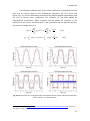
Fig. 6 Representation of a rectangle function through the Fourier series and the
sinusoids that form it. With 1, 3, 5 and 51 terms. ...........................................................13
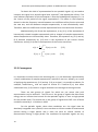
Fig. 7 The finite signal
and its discrete Fourier transform
. ..............................19
Fig. 8 Circular convolution of two rectangular sequences of length . ..........................22
Fig. 9 Circular convolution of
and
with zero-padding. It is equivalent to the
linear convolution of the original signals. .......................................................................23
Fig. 10 Example of the application of the zero-padding to achieve the linear
convolution through the circular convolution as it is used in the application developed
in this thesis. ....................................................................................................................24
Fig. 11 Result of the circular convolution of the filter
and every
. After the
overlapping,
is effectively filtered. ..........................................................................25
Fig. 12 Example of bit-reversal with 3 bits. .....................................................................27
Fig. 13 Kaiser window with
and
. ....................................................30
Fig. 14 Precision requirements. .......................................................................................34
Fig. 15 Output requirements. ..........................................................................................35
Fig. 16 Creativity requirements. ......................................................................................35
Fig. 17 Clarity requirements. ...........................................................................................36
Fig. 18 Cyclic data processing. .........................................................................................38
Fig. 19 Basic layout of the application. ............................................................................43
v
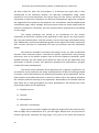
Fig. 20 Flow of the states for 2-states manipulations. The green arrows represent a
manipulation’s button click and the red ones a click on the reset button. ....................47
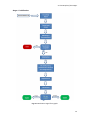
Fig. 21 Flow of the states for 3-states manipulations. The green arrows represent a
manipulation’s button click and the red ones a click on the reset button. ....................48
Fig. 22 Harmonic creation method. The value of the amplitude of the last sample is
between that of the first and second samples. ...............................................................50
Fig. 23 Example of the filter manipulation. .....................................................................51
Fig. 24 Example of the equalizer manipulation. ..............................................................52
Fig. 25 Situation 1: no manipulation ...............................................................................60
Fig. 26 Situation 2: applying a filter of order N = 396 .....................................................60
Fig. 27 Situation 3: applying filter and equalizer. Also synthesizer from around loop
number 20 onwards ........................................................................................................61
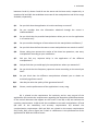
Fig.28 Survey results: questions 1 and 2 .........................................................................64
Fig.29 Survey results: questions 3, 4 and 5 .....................................................................65
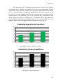
Fig.30 Survey results: questions 6 ...................................................................................65
Fig.31 Survey results: questions 7, 8 and 9 .....................................................................66
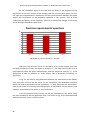
Fig.32 Survey results: questions 10 and 11 .....................................................................67
Fig.33 Survey results: question 12 ...................................................................................67
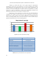
Fig.34 Survey results: requirements average. .................................................................68
Fig. 35 Initialization stage’s flow graph. ..........................................................................73
Fig. 36 Data acquisition stage’s flow graph .....................................................................74
Fig. 37 Spectrum manipulation and spectrum management stages’ flow graph. ..........75
Fig. 38 Playback and visualization stage’s flow graph .....................................................76
vi
List of Tables
Table 1 Common sampling rates for digital audio ..........................................................10
Table2 Priorities of the requirements .............................................................................37
Table3 Distribution of the requirements by stages. The symbol “+ +” means that the
requirement is mainly fulfilled in that stage, and the symbol “+” means that only some
details of that requirement are met in that stage ..........................................................39
Table 4 Summary of the fulfilment of each requirement ...............................................68
vii
Agraïments
M’agradaria agrair als professors Horst Eidenberger i Xavier Giró-i-Nieto que m’hagin
brindat la oportunitat de realitzar un projecte final de carrera que m’ha permès, per
una banda, unir les telecomunicacions amb una de les meves grans passions com és la
música, i per l’altre, fer les primeres passes en el món del processament digital
d’àudio. També agrair-li a la UPC i a la TU Wien que hagin fet possible la meva estada
Erasmus a Viena.
Donar les gràcies especialment al meu amic i ex-company de carrera Eduard
Valera i al meu cosí Guiu Llusà perquè si aquest projecte té cara i ulls és en gran part
gràcies als seus consells.
Agrair també a tots els amics i amigues que m’han acompanyat durant els
anys d’universitat i que espero que d’aquí molts més encara siguin al meu costat.
Per últim, una menció especial als meus pares per aclarir-me sempre les idees
i ajudar-me a tirar endavant en els pitjors moments.
viii
Acknowledgements
I would like to thank Professor Horst Eidenberger and Professor Xavier Giró-i-Nieto, on
one hand, for providing me the opportunity to carry out a master thesis that allowed
me to unite the telecommunications engineering with music, which is one great
passion of mine, and on the other hand, for allowing me to make the first steps into
digital audio processing. Also, I have to thank UPC and TU Wien for making my Erasmus
stay in Vienna possible.
I want to express my gratitude to my friend and former career colleague
Eduard Valera and to my cousin Guiu Llusà because if this project does make any
sense, it is to a great extent thanks to their advice.
I also want to thank the friends that have accompanied me during the
university years and that I hope will be by my side for many more years to come.
Finally, I want to show my gratitude to my parents for clarifying my thoughts,
and also for helping me in the worst moments.
ix
Abstract
In view of the growth of the market of devices such as tablets and smartphones and
the increasing popularity of the electronic music, in this project we develop an
application that mixes both phenomena. Specifically, it allows the user to modify a
previously existing wave file in real-time thorough the manipulation of its frequency
spectrum. The entire process is performed on a tablet computer.
Firstly, the data is extracted from the file in pieces of a certain length that can
vary depending on the situation. These pieces, which become our signal, are
transformed using a fast Fourier transform algorithm and their spectrum is
manipulated by the user through tapping. After this, we inverse transform the
modified signal to play it and subject its spectrum to some processes that improve its
visualization, which is synchronized with the playback.
We establish a set of requirements that must be fulfilled, which are related to
the accuracy in the application of the modifications and the precision and immediacy
of its results, the quality of the output, the level of creativity that the user can achieve
and the clarity of the contents of the application.
The results show that the application fulfils remarkably well every
requirement related to the technical aspects and accomplishes its purpose preserving
the quality of the original file. Even though the creative possibilities of this first
prototype are limited, we consider that the improvement margin is big for further
development.
x
1
Introduction
It was in 1977 that music started walking its way into the digital era. That year took
place what is considered to be the first commercial digital recording experience in the
U.S., and from there we have witnessed a fast evolution of the methods and
technology to digitalize and store music with the consequent increase of the quality of
the result. This way, over the last decades, the digital representation of music has been
gaining ground to the analogue methods at a fast pace.
But the technology surrounding music is not the only thing constantly
evolving, also the music itself does, and most of the times one influence the other. The
electronic music is the latest result of this evolution and is deeply influenced by the
developments in the recording, storage and also manipulation, through devices such as
synthesizers, of music. Lately, this music genre and the DJs that play and compose it
are gaining a lot of popularity and a larger share of the music delivery, as the new
generations of consumers embrace them.
Regarding the storage of music in a digital form, in the last decade internet
claimed its superiority over hardcopy supports such as compact discs. At that time, the
only way to have access to this big amount of music was through computers, but this
has changed with the emergence of the smartphones and tablets a few years ago. In a
similar tendency to that of the electronic music and DJs, people increasingly choose to
purchase this kind of devices, at the expense of PCs and laptops, making their market
rapidly extend.
We have built our application with the idea to satisfy these two growing
markets. In the next section we will establish the motivations that encouraged us to go
ahead with this thesis and the goals that we set for ourselves.
1
Interactive Spectral Manipulation of Music on Mobile Devices in Real-Time
1.1 Motivation
In this thesis we aim to create the prototype of an application for tablets that attempts
to mix the two growing social phenomena mentioned before. We want this application
to allow us to manipulate an already existing source of sound in real-time, in a way
resembling that of a DJ. However, we expect to do this in the frequency domain, i.e.,
through the modification of the coefficients of its spectrum.
Ideally, we want the user to be able to interact in an intuitive way with the
application, and also the application to enhance the creativity of the user through a
variety of manipulation options as flexible as possible and with the ability to combine
with each other. In the next section we will introduce two examples of software to try
to define the current state of the possibilities in sound manipulation.
1.2 Related software
In this section we are going to analyse and summarize the features of two different
projects: Reactable and AudioSculpt. The first one is an application for tablets designed
to be intuitive and easy to use in order to maximize our creativity. The second one is a
computer program with more of an academic facet that enables us to thoroughly
analyse sound and to process it in many sophisticated ways. It is easy to see that the
Reactable project has goals much more similar to ours than AudioSculpt, but
AudioSculpt’s interaction with the sound resembles much more that of our application.
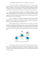
Reactable is based on the homonymous electronic musical instrument and it
consists of a circular luminous surface where we can place objects with different
shapes related to their functionality in sound generation or in effect processing to
produce sound. The surface will show interactive graphics and animations showing
relevant information and the possibility to access more advanced configuration menus.
2
1. Introduction
Fig. 1 Reactable application view
There are four types of objects: the generators that produce the sound and
have a square shape; the effects that modify this sound and have a rounded square
shape; the controllers that send control values to other objects and have a circular
shape; and the general controllers that modify the general behaviour of the
application. We can create music by moving and relating these objects.
The generators are the most essential type of object because without them
there is no sound. There are four types of generators each one with a different way to
create sound. We can generate basic signals such as sinusoidal or square waves while
choosing its frequency and amplitude, play instruments stored in a sample bank,
repeatedly reproduce sound files or take the sound from an external source.
Fig. 2 Reactable oscillator object
3
Interactive Spectral Manipulation of Music on Mobile Devices in Real-Time
To process and modify the generated sound there are the objects named
effects. With them we can filter the sound modifying its frequency response, delay or
repeat it, modulate it, and also change its shape. By rotating the objects, we are able
to change the value of its main parameter, for example, the duration of the delay. The
interaction with the graphics around it allows us to modify the intensity of the effect.
There is a type of object that allows us to modify the behaviour of other
objects, manipulating sound in an indirect way. This is the job of the objects named
controllers. With them we can apply cyclical variations to the generated sound, create
sequences that will be passed to the generators and even control them from and
external device such as a midi keyboard.
There is a special kind of controllers, named general controllers, which affect
the instrument as a whole, i.e., we are able to modify the output sound of all the
objects at once. For example, we can change the volume, the tempo or the tonality of
the sound; modify the background of the application, etc.
When compatible objects are positioned close to one another a connection
between them appears automatically as they start to interact with each other. Audio
connections are graphically represented by the sound waves that pass through them,
i.e., the values of the data being transferred from one object to the other in real-time.
These connections can be temporarily muted by breaking the connective link between
them.
Fig. 3 Types of objects and connections
All these objects, graphics, animations and the possibilities that they offer as a
whole, result in an intuitive and direct way to create music. The application is easy and
fun to use and regarding the performance, it doesn’t fall behind with the actual
instrument which has been already used by famous musicians like Björk and renowned
DJs like Gui Boratto.
4
1. Introduction
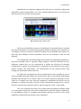
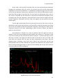
AudioSculpt is a computer program with which we can visualize, analyse and
manipulate sound in great detail. It is a very complex software and in this section we
will only summarize its main functionalities.
Fig. 4 AudioSculpt program view
There are three different types of visualization of the sound. We can visualize
the sound’s waveform, the sound’s instantaneous frequency spectrum or visualize it as
a sonogram. Each one of these visualizations allows us to manipulate the sound in its
own way with different control parameters and can be zoomed in and out and
browsed.
The manipulation and processing of the sound can be graphically applied in a
way that resembles that of a graphic design program, with the definition of timefrequency regions that can be transformed. It allows the filtering of individual
components or regions, the compression or expansion of the duration of the sound,
timbre creation and modification, the improvement of the signal-to-noise ratio
through the elimination of the noise, etc.
To follow the consequences of the transformations that we apply or just to
collect valuable information about the sound that we want to manipulate, AudioSculpt
provides several tools for its analysis. We can see each frequency component of the
sound as it changes over time and this component’s amplitude and phase; we can
estimate the spectral envelope; we can find the fundamental frequency of a sound;
these are some of the most basic options, but the program’s offer is much wider.
This very complete and precise set of tools and the graphical interface allow
us to have great control over the sound. Combining this with the options available for
its manipulation results in a program that boosts creativity and that can be really
helpful for professional and amateur music composers.
5
Interactive Spectral Manipulation of Music on Mobile Devices in Real-Time
1.3 Challenges
The application defined in Section 1.1 is our goal, and we want to get as close as
possible to it. As we said, in this thesis we want to build a prototype of this application.
To do that, we start establishing the challenges that we have to overcome. There are
basically three of them.
The first one is related to the capacity of the tablet to work with heavy
calculation processes such as the Fourier transform. Specifically, we must create an
application that is technically able to endure several Fourier transforms and the same
amount of inverse Fourier transforms every second, and optionally apply some
modifications to the frequency spectrum coefficients to be able to obtain a different
audio in the output preserving the quality of the original file. Moreover, it must
provide decent results for aspects such as the response time to the user actions or the
accuracy of the application and the results of the different manipulations.
Secondly, the application must be as intuitive and helpful as possible in order
to easily analyse and manipulate the spectrum. We will have to find out, for instance,
the most appropriate way to represent the amplitude of each coefficient of the
spectrum, the most fitting scale for the frequency axis, a proper way to apply and
control the different manipulations available, etc.
This leads us to the third challenge, which is to implement ways to modify the
sound through the manipulation of the spectrum that are interesting in the sense that
they are either useful or artistic. Now that we have stated the aims of the thesis, it is
time to briefly introduce its contents.
1.4 Overview of the following chapters
The structure of the thesis will be the following: in Chapter 2 we will include all the
theory background necessary to fully understand how the application works starting
with a brief description of the digital representation of the sound in general the
particular case of the wave format.
After that we will split the theory behind the Fourier transform into five
different sections: the first one explaining the continuous Fourier series and transform,
the second introducing the discrete Fourier series and the discrete-time Fourier
6
1. Introduction
transform, the third describing the discrete Fourier transform, the forth addressing a
fast Fourier transform algorithm, and finally, the fifth outlining some of its
applications. To finish Chapter 2 we will provide mathematical theory about two of the
tools used in the application that we think need to be detailed.
To start Chapter 3, we will state the requirements for the application. This will
lead, firstly, into the description of some general ideas of what the application should
accomplish, and then into a general exposition of the selected approach and its
relation with the requirements.
The actual implementation of the application will be thoroughly described in
Chapter 4 and some diagrams of the processes of the application will be provided. We
will also discuss the decisions we have taken to solve the problems that we have
encountered during the implementation.
Chapter 5 will deal with the evaluation of the application. First of all, we will
describe its performance objectively, discussing the most relevant technical data, such
as execution times, delays, time and frequency resolution values, etc. After that there
will be a section dedicated to the users’ feedback.
Finally, we will place the conclusions, where we will synthesize the contents of
the thesis, reflect on the challenges that we stated in the beginning and discuss the
achievements and limitations of the thesis; and the future work, where will devote
some lines to debate the possibilities for future research.
7
2
Background
In this chapter we will explain all the theory necessary to fully understand how the
application developed in this thesis works. First, Section 2.1 will describe the digital
representation of sound. We narrow the explanations as much as possible taking into
account that the application works with the wave format.
In Section 2.2 we will define the Fourier series and the Fourier transform for
continuous signals and we will describe how the transform is derived from the series.
In Section 2.3 we will follow the same process for the discrete Fourier series and the
discrete-time Fourier transform. Section 2.4 will be devoted exclusively to the
explanation of the discrete Fourier transform and the properties that can help us the
most in the application. One of the efficient algorithms to compute the discrete
Fourier transform called fast Fourier transform algorithms will be described in Section
2.5. To close the group of sections related to the Fourier transform, in Section 2.6 we
will mention some of its applications. After this, in Section 2.7, we will introduce the
theory regarding the filters that we use, and finally, in Section 2.8, we will present a
frequency interpolation technique.
About the notation used in this chapter, it is important to remind the reader
that we always express the discrete Fourier transform of a finite signal or the discrete
Fourier series of a periodic signal, with its same letter in uppercase and the same subindex. Moreover, periodic signals are denoted with the letter and finite signals with
the letter .
8
2. Background
2.1 The representation of sound
As sound in a digital form is the raw material of the application, we deemed necessary
to briefly explain how we digitally represent it. A suitable definition of sound for our
purposes could be: an analogue, time-varying, real-valued signal. Obviously, this is not
the most appropriate type of signal to work with devices such as computers, tablets,
smartphones, etc. To make it more suitable we need to digitize it.
A way to digitize a signal is to take samples of it. The process of sampling
consists in giving a numerical value to the amplitude of the signal in a precise instant.
To do this, we need to consider the sampling rate, i.e., how many samples we take
every second, the bit depth, i.e., the number of bits that we use to represent every
amplitude value, and also how we assign the numerical values to the amplitude of the
signal.
2.1.1 Sampling rate and bit depth
There are some standardized values for the sampling rates: 8 kHz for the telephone
communications or 44.1 kHz in the case of audio signals, but also 11 kHz, 22.05 kHz,
etc. To understand what implies to use one sampling rate or another we need to know
that the human ear frequency range goes from about 20 Hz to about 20 kHz and to
take into account the Nyquist-Shannon sampling theorem.
This theorem states that in order to be able to perfectly reconstruct a signal
after a process of sampling, the signal must be band limited and the sampling
frequency must at least double that limit. Otherwise, an effect known as aliasing
appears, distorting the signal and thus reducing its quality [3].
Knowing that we cannot hear any frequency higher than 20 kHz, we can force
it to be the highest frequency in the signal through a process that involves filtering.
After that, and following the theorem, we can set a sampling rate that, at least,
doubles this frequency value. This would be the standardized sampling rate of 44.1 kHz
used to sample audio signals. Of course, if we don’t need the highest quality, we can
use a lower sampling rate as it is done in many cases. To avoid the aliasing we just
need to previously limit the signal’s frequency range to half the chosen sampling rate.
9
Interactive Spectral Manipulation of Music on Mobile Devices in Real-Time
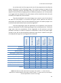
Sample rate Quality level
Frequency range
11,025 Hz
Poor AM radio (low-end multimedia)
0–5,512 Hz
22,050 Hz
Near FM radio (high-end multimedia)
0–11,025 Hz
32,000 Hz
Better than FM radio (standard broadcast rate) 0–16,000 Hz
44,100 Hz
CD
0–22,050 Hz
48,000 Hz
Standard DVD
0–24,000 Hz
96,000 Hz
High-end DVD
0–48,000 Hz
Table 1 Common sampling rates for digital audio1
As we have said before, we also need to define how many bits we should use
to represent the amplitude value of every sample. The more bits we use, the more
levels we will have to approximate the signal, reducing the error in every
measurement. This ensures a better quality but also a bigger amount of data for the
same information. The typical values are 8, 16, 24 and 32 bits per sample and the
number of levels will be , where is the number of bits used.
The representation of the amplitude of a digital signal can be expressed in dB
relative to its full scale, i.e., dBFS. In this case, the maximum amplitude value is 0 dBFS
and corresponds to a signal that covers all the levels available. Therefore, a signal
whose amplitude is within one level has the lowest possible amplitude value. For
instance, a signal with 16 bits per sample has a range of amplitude that goes from 0
dBFS to -96.33 dBFS.
(
)
2.1.2 Quantization
The wave files allowed by the application use a format named linear pulse code
modulation to assign the levels to the amplitude values of the signal. This format
distributes the levels in a linear way, i.e., we divide the amplitude range of the signal
we are sampling in as many parts as levels we have, in a way that every pair of levels is
separated by the same distance [13][14]. The range of the values of the levels
1
Table extracted from http://goo.gl/c0xgny. Last access: June 2014.
10
2. Background
)
is (
. The distance between levels is defined as the quotient of
⁄ .
the amplitude of the signal and the number of levels, i.e.,
We will assign to each sample the value of the level that is closest to the signal
in that instant. It is in this assignation that we introduce errors. The error committed
⁄
⁄ .
will be comprised between
Fig. 5 Sampling of a signal with
bits.
levels linearly distributed.
2.1.3 The signal
Until now we know that the signal we use is a discrete signal. Before advancing to the
next sections, we must define it a little bit more. As we have stated in Section 1.1, we
want to manipulate the signal in the spectral domain, and therefore, we need to use
the Fourier transform to compute its spectrum. To be able to both analyse the
frequency contents of this signal and modify them in real-time, it is not useful to apply
the Fourier transform to the entire signal at once. In Subsection 2.4.2, we refer to the
frequency and time resolutions and this helps us understand that we need to cut the
song into small pieces and apply the Fourier transform to each one of them separately.
As a consequence, our signal will be limited in the time domain. If we recall that the
range of values that our signal can take is also limited, then we can assume that the
signal is of finite energy. After these clarifications, we can state that the signal we work
with is a discrete aperiodic signal of finite energy.
In the next sections we introduce the Fourier series and transform in its
continuous and discrete versions, its properties, and many other concepts that help us
understand the behaviour and characteristics of this signal in the frequency domain.
11
Interactive Spectral Manipulation of Music on Mobile Devices in Real-Time
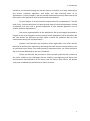
2.2 The continuous Fourier series and transform
The usage of a sum of harmonically related sinusoids to represent periodic phenomena
takes us back to civilizations that existed thousands of years ago. Much more recently,
mathematicians and physicists such as L. Euler or D. Bernoulli kept developing this
idea, and their discoveries were the base for the work of Jean Baptiste Joseph Fourier,
who was the first to affirm that any periodic signal could be represented by a sum of
sinusoids or complex exponentials, i.e., by what is now known as its Fourier series.
Furthermore, he obtained a method to extend this kind of representation to aperiodic
signals. This method requires not a sum but an integral of complex exponentials, which
no longer need to be harmonically related. This is J. B. Fourier’s main contribution to
the fields of mathematics, physics and science in general, and it is named the Fourier
transform [1].
But these results were not uncontested. As an example, the renowned
scientist J. L. Lagrange was against them. He argued that no signal with a discontinuous
slope could be exactly represented by a sum of sinusoids [1]. This is actually true, but it
has not prevented the Fourier series and the Fourier transform to become incredibly
useful tools in a very wide range of disciplines such as mathematics, science and
engineering.
2.2.1 Definition
As we have said before the Fourier transform originates from the same idea as the
Fourier series: representing a signal through a weighted summation of complex
exponentials of different frequencies; and the result is conceptually the same: a
function that indicates the amplitude of every complex exponential that forms the
signal, i.e., the frequency spectrum of the signal.
In the case of the Fourier series, which only applies to periodic signals, the
complex exponentials used for the representation are harmonically related. This
means that their frequencies are all multiples of a fundamental frequency , which is
⁄ . Therefore, the Fourier
defined as the inverse of the period of the signal
series of a signal is a discrete and infinite sequence of coefficients, as there are only
amplitude values for the complex exponentials corresponding to these specific
frequencies and an infinite number of multiples of the fundamental frequency.
12
2. Background
In the frequency domain each one of these coefficients is separated from the
next one an interval equal to the fundamental frequency. Eq. (2.1) shows the
signal ( ) as a linear combination of harmonically related complex exponentials, and
eq. (2.2) its Fourier series coefficients. The constant ⁄ has been added for
mathematical convenience. Other constants will be added, for example, in the
equations of the Fourier transform both in the continuous and the discrete versions,
but we will no longer refer to it.
( )
∫
∑
( )
∑
∫
( )
(
)
(
)
Fig. 6 Representation of a rectangle function through the Fourier series and the sinusoids that
form it. With 1, 3, 5 and 51 terms2.
2
Figure extracted from http://www.ee.nmt.edu/~wedeward/EE212/SP08/example6.html. Last access:
June 2014. The figure has been modified.
13
Interactive Spectral Manipulation of Music on Mobile Devices in Real-Time
To obtain this kind of representation for an aperiodic signal ( ) we need to
interpret this signal as a periodic signal with a period that approaches infinity. The
most obvious implication of this assumption is that the fundamental frequency , as
the inverse of the period of the signal, approaches . The effect in the frequency
domain is that the frequency interval between one coefficient of the Fourier series and
the next one, and also between complex exponentials, is now infinitesimally small.
Therefore, both the coefficients and the exponentials form now continuous functions.
Mathematically, this forces the replacement, in eq. (2.1), of the summation of
harmonically related complex exponentials with an integral of complex exponentials,
whose frequencies are infinitesimally close. Therefore, the equations eq. (2.1) and eq.
(2.2) become respectively eq. (2.3) that is the expression of the inverse Fourier
transforms, and eq. (2.4) that is the expression of the Fourier transform.
( )
( )
∫
∫
( )
( )
(
(
)
)
2.2.2 Convergence
It is important to notice that we are assuming that ( ) can be always represented by
a linear combination of complex exponentials, and that is not true. Actually, as a result
of applying the equations eq. (2.2) and eq. (2.4) to a signal, it is possible to obtain, for
example, coefficients
that are equal to infinite or a function ( ) that when
substituted in eq. (2.3) results in a signal that does not converge to the original one.
There are two groups of signals for which we can assure that such
representation can be achieved. The first one is the group of signals that have finite
energy over an infinite time interval for the aperiodic signals, or over a single period
for the periodic ones. The second one is the group of signals that fulfil a set of three
conditions stated by P. L. Dirichlet in 1829.
For the periodic signals, these three conditions are: the signal must be
absolutely integrable over a period; it must not have an infinite number of maxima and
minima during a single period; and it must not have an infinite number of
discontinuities during a single period. The conditions for aperiodic signals are very
14
2. Background
similar. The only differences are that the first condition must apply for an infinite time
interval and conditions two and three for any finite time interval.
In the last paragraph we have described the conditions for a signal to have its
own Fourier transform, but it is necessary to explain that some signals that do not fulfil
all of these conditions, such as periodic signals like the rectangle function, can be
considered to also have a Fourier transform. In the end a great amount of signals,
including the most common and useful, do have a Fourier transform and this is why it
is so widespread among many different disciplines.
2.3 The discrete Fourier series and the discrete time
Fourier transform
Both the discrete Fourier series and transform have many similarities with their
continuous counterpart: the idea of representing a signal with a linear combination of
complex exponentials remains the same; the discrete Fourier series applies only to
periodic signals and the transform extends the representation to the aperiodic signals;
and the way to derive the discrete-time Fourier transform from the discrete Fourier
series is equivalent to the continuous case.
We must understand the digital signal as the sampled version of a continuous
signal, and therefore, we need to introduce two concepts: the sampling frequency ,
i.e., how many samples of the continuous signal we are taking each second, and the
time between samples , i.e., the sampling period, which is the inverse of the
sampling frequency. One of the differences from the continuous case lies in the
notation and is a result of the appearance of the sampling frequency. We now denote
as or the frequency normalized to . If the frequency is not normalized, we
write .
It is important to distinguish between the two different kinds of Fourier
transform that exist for discrete signals: the discrete-time Fourier transform, which
applies to discrete signals but results in a continuous function in the frequency
domain; and the discrete Fourier transform, for which both the signal and the resulting
function are discrete.
The basic difference is that now the signal is discrete. This difference forces
some changes in the equations due to the variation of the mathematical behavior of
15
Interactive Spectral Manipulation of Music on Mobile Devices in Real-Time
the complex exponentials, and also creates some difficulties in processing and
analyzing the signal that we will need to overcome.
2.3.1 Definition
The fact that the signal is now discrete due to the sampling process means that it only
has values for the time instants that fulfil
. This way the integral in eq. (2.2) and
eq. (2.4) becomes a summation, and the complex exponential suffers the same
discretization process when multiplying the signal. Also, if the signal is periodic, its
period is measured in samples and not in time, and it is equal to and not . This way,
⁄ , as its inverse, are
both the period and the fundamental frequency
independent from the sampling frequency.
As we can see in eq. (2.5), when the complex exponentials become discrete in
the time domain with a time interval between samples equal to , they automatically
become periodic in the frequency domain with a period equal to the . In other
words, the discretization limits the highest frequency that they can reach to
.
We can also express their period either as
or
. Additionally, the
periodicity of the complex exponentials forces both the discrete Fourier series and the
discrete-time Fourier transform, i.e., the signal’s frequency spectrum, to be periodic as
well.
(
)
(
)
(
)
(
)
The number of different complex exponentials that are harmonically related
to a fundamental frequency inside any finite frequency interval is also finite. This
means that, unlike the Fourier series for continuous signals, the discrete Fourier series
is a finite sequence of coefficients, whose equation is shown in eq. (2.7). To be more
precise, what is really finite is the number of coefficients that we need to
represent
in eq. (2.6). However, eq. (2.7) is, as we have explained, periodic with
period , and therefore not finite.
∑
∑
〈 〉
∑
〈 〉
16
(
)
(
)
〈 〉
∑
〈 〉
2. Background
To derive the discrete-time Fourier transform equations from the equations of
the discrete Fourier series we need only to follow a process homologous to the
continuous case. That is, to interpret an aperiodic and finite signal
as a periodic
signal with a period
that goes towards infinite. Again, the consequences of this
assumption are that the fundamental frequency
approaches and that the
frequency interval between one coefficient of the discrete Fourier series and the next
one, and also between complex exponentials, becomes infinitesimally small. Thus,
both the coefficients and the complex exponentials result in continuous functions.
Despite these changes, the complex exponentials are still periodic with
period
, and therefore, we only need to integrate over this interval to achieve
the representation of
as we can see in eq. (2.8), which is the equation of the
inverse discrete-time Fourier transform. It is easy to see that eq. (2.7) becomes an
infinite summation resulting in eq. (2.9), which is the equation of the discrete-time
Fourier transform.
∫
( )
∑
( )
(
(
)
)
2.3.2 Convergence
The convergence of the discrete Fourier series representation to the signal
is
guaranteed by the fact that, both in eq. (2.6) and eq. (2.7), the summation is limited to
a finite number of terms , and because
, as the result of a sampling process,
includes only finite values. In eq. (2.9) there is a summation of infinite terms, but we
defined
as a finite signal and therefore, assuming again that
contains only
finite values, the discrete-time Fourier transform has no problems of convergence.
However, extending the study to aperiodic signals of infinite duration, the convergence
of the discrete-time Fourier transform is only guaranteed if
is absolutely
summable in an infinite interval samples or if it is of finite energy.
17
Interactive Spectral Manipulation of Music on Mobile Devices in Real-Time
2.4 The discrete Fourier transform
Up until now, for the case of the aperiodic signals, we have been able to obtain only a
continuous spectrum. Through the Fourier transform, when the signal is continuous or
through the discrete-time Fourier transform, when it is discrete. Nowadays, we usually
need a discrete version of the spectrum to be able to work with digital devices. We will
achieve that through the discrete Fourier transform of the signal.
2.4.1 Definition
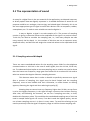
We can define the discrete Fourier transform of a finite signal
of duration as
one period of the discrete Fourier series of a periodic signal
, whose period is
.
We can also interpret it as on period of a sampled version of its discrete-time Fourier
transform, with one sample separated from the next one by a frequency interval equal
⁄ [2].
to
Both ways result in one period of the same periodic discrete signal. Eq. (2.10)
corresponds to the inverse discrete Fourier transform, and eq. (2.11) to the discrete
Fourier transform of the signal
. Notice that if the discrete Fourier series does not
have any convergence issues, neither does the discrete Fourier transform, as this
transform is essentially one piece of the discrete Fourier series.
{
{
∑
〈 〉
∑
(
〈 〉
∑
〈 〉
)
(
)
We cannot forget that in eq. (2.11) we are extracting one period from the
discrete Fourier series of
. The reason why we can substitute
for
is that
they are equal over the interval that we are summing. Another conclusion that we can
draw from these equations is that both
and
have the same number of
samples.
18
2. Background
Fig. 7 The finite signal
and its discrete Fourier transform
.
2.4.2 Properties
This last kind of Fourier transform is the one we use in this thesis because of its digital
orientation. It shares some properties with the rest of the Fourier transforms, but it
has some of its own too. In this section we focus on the properties that are relevant for
the processes of the application. We describe them in a general way, and in some
cases, we also explain how they are specifically used in the processes of the
application.
In the introduction of this chapter, we already referred to the notation, and
everything written there is still valid. However, to be able to correctly explain all the
properties in this section in a general way, and also describe their specific use in the
application, we need to do some more clarifications.
For the general or purely theoretical description of a property, we use
numerical values for the sub-index of the signals. These signals are arbitrary signals
that fulfil the conditions that we specify in every case. On the other hand, when we
start describing the role of these properties in the application, we need to give a name
to the signals that take part in its processes.
19
Interactive Spectral Manipulation of Music on Mobile Devices in Real-Time
We represent the entirety of the data inside the wave file as
. As we said
in Subsection 2.1.2, we need to cut this signal into smaller signals. We name
them
, where
is a sub-index that starts as and increases with every cut
of
.
Symmetry
Taking into account the symmetry of the signals we work with can sometimes
be really useful, in the sense that it can greatly decrease the complexity of an
algorithm, increase its efficiency, etc. The nature of a signal in one domain can
determine the symmetry in the other domain, for instance, the fact that a signal
is real-valued has an impact in the symmetry of its spectrum. Specifically, the
equations below show the symmetries obtained in the frequency domain for a realvalued signal
and an imaginary-valued signal
, both of length .
Linearity
A basic property of all the Fourier series and transforms is the linearity. In the
case of the discrete Fourier transform we can say that the transform of a linear
combination of two finite discrete signals is equal to a linear combination of the
transforms of the two signals with the same coefficients.
It can happen that the duration of
and
is not the same. It is
obvious that
has the duration of the longer of these two signals. In order to
sum
and
correctly, i.e., to sum the coefficients that correspond to the
same frequency, we need both of them to be of the same duration. Therefore, before
transforming them, we need to fill the shortest one with zeroes until it reaches the
other one’s duration. This way, the duration of
coincides with that
of
,
and
. This technique is called zero padding and it is of great
importance for the application as we will see with the following properties.
20
2. Background
Time - frequency resolution
In the discrete Fourier transform, is the number of samples of the signal
that we want to transform and therefore marks its duration in the time domain.
Additionally, it is the number of coefficients of the discrete Fourier transform of this
signal, i.e., the number of frequencies that we can detect in the signal.
In the application, the actual value that receives is greatly influenced by the
algorithm that we use to compute the discrete Fourier transform, which leaves us with
only a few options. However, in this section we do not take this into account, and we
focus on the effect of the value of on the time and frequency domains.
Giving a high value results in a good frequency resolution and a bad time
resolution, i.e., we can detect many different frequencies, but we are not able to
precisely tell in which instant they appear. On the contrary, a low value of limits the
number of frequencies, but allows us to precisely know the instant they appear. There
is no such thing as the correct value of , it depends on many factors and it varies with
every different application of the discrete Fourier transform.
The specific case of the application is the following: the signals
have a
fixed duration , but it is not mandatory for them to be completely filled by samples
of
. We may need to place a variable number of zeroes at the end of the signal to
guarantee the correct application of a filter. This implies that the frequency resolution
always remain the same, i.e.,
has coefficients in any situation, but the time
resolution can vary depending on the number of samples of
that we include in
every
. Specifically, the fewer samples we include the better the time resolution
is.
One of the handicaps of having only a limited amount of complex
exponentials to represent a signal is that, if this signal contains frequencies that do not
match with those of the complex exponentials, we have to use a combination of these
functions to represent these frequencies. This usually results in a contamination of the
spectrum that consists in the appearance of low coefficients in the high frequencies.
The lower the value of the stronger is this problem.
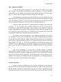
Circular convolution
Another property influenced by the periodic background of the discrete
Fourier transform is the kind of convolution that applies to it: the circular convolution.
We will denote it with an inside a circle as we can see in Fig. 8. The same way that
we obtain the discrete Fourier transform from the discrete Fourier series by cutting off
21
Interactive Spectral Manipulation of Music on Mobile Devices in Real-Time
one period, we can extract the circular convolution from the discrete Fourier series’
periodic convolution. Therefore, let us first introduce this concept.
The periodic convolution is the convolution of two periodic signals
and
with a period of duration
and
and equal to the finite sequences
and
respectively. This convolution is also periodic, with period
{
}. Unfortunately, it doesn’t correspond to a periodic version of the linear
convolution of
and
, because the duration of this linear convolution would
be
which is different from
or , unless one of them is equal to . In
any other case, some of the samples of this linear convolution overlap with the linear
convolution of the two signals’,
and
, subsequent period. The periodic
signal
formed this way is the periodic convolution of these two signals and we
define
as its discrete Fourier series.
∑
If we extract one period of
we obtain
, which is the result of the
circular convolution of
and
. To be able to express
as a function of
these two finite signals we need to introduce the concept of modulo . To do this we
take
, which is the periodic version of the finite signal
, as an example.
Fig. 8 Circular convolution of two rectangular sequences of length .
22
2. Background
∑
We observe that the circular convolution of
and
in the time
domain is expressed in the frequency domain as the multiplication of their discrete
Fourier transforms. To do this multiplication correctly, both transforms must have the
same number of samples. This way only the coefficients corresponding to the same
frequencies multiply each other. To achieve this we need to apply the zero padding
technique to the shortest signal in the time domain until it reaches the duration of the
other one. As a result,
and
have the same duration, and therefore, also
does
.
Fig. 9 Circular convolution of
and
with zero-padding. It is equivalent to the linear
convolution of the original signals.
Notice that the result obtained in the time domain by the multiplication
of
and
in the frequency domain is only correct if these signals are periodic
in the time domain, i.e., if
and
are truly one period of
and
respectively. This happens because they are automatically interpreted as such by the
circular convolution. Otherwise, to obtain the correct result for this multiplication, we
23
Interactive Spectral Manipulation of Music on Mobile Devices in Real-Time
need to prepare beforehand the signals
and
. Assuming that they have
duration
and
respectively, the preparations consist in extending both of them,
with the technique of the zero padding, until their duration become equal to
. This way we make sure that both signals have the same duration in the
frequency domain, which is necessary to multiply them, and that this duration matches
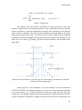
that of the linear convolution of the original signals avoiding the overlap.
In the application, when we perform the filtering with a filter
of
duration
of the signal
, i.e., of consecutive
signals, we apply the filter in
the frequency domain multiplying
by
, but we need to prepare both signals
in the time domain before we transform them.
Specifically, we need to fill
with
samples of
and zeropad the last
samples. We also must extend
, again zero-padding, until it
reaches duration . As a consequence, both
and
have duration
and
therefore, their linear convolution
has duration
. However, because of the
zero-padding, its last samples are equal to zero, and that is why we can consider it
to have also duration .
Fig. 10 Example of the application of the zero-padding to achieve the linear convolution
through the circular convolution as it is used in the application developed in this thesis.
24
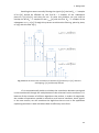
2. Background
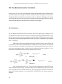
Recalling that we are actually filtering the signal
, the last
samples
of
should be affected by the first
samples of the subsequent
piece
of
, and they are not. To solve this problem, we just need to
overlap the last
samples of one
with the first
samples of the
subsequent (
. Through this process we achieve the filtering, piece by piece,
)
of
with the filter
.
Fig. 11 Result of the circular convolution of the filter
and every
overlapping,
is effectively filtered.
. After the
If it is computationally viable to calculate the convolution between two signals
in the time domain through the multiplication of their discrete Fourier transforms, it is
because of the existence of efficient algorithms that reduce, in orders of magnitude,
the number of operations needed to transform, and inverse transform, these signals.
In the next section, we will introduce the algorithm that we use in the application
explaining how does it work and where does its efficiency come from.
25
Interactive Spectral Manipulation of Music on Mobile Devices in Real-Time
2.5 The fast Fourier transform
Despite Gauss discovered the first one in 1805, the efficient algorithms for the
calculation of the discrete Fourier transform, now referred to as fast Fourier transform
algorithms, did not become useful until the emergence of the digital technology. The
reason why is that these algorithms truly shine when the number of samples to
transform exceeds human capacity to use them.
2.5.1 Definition
Normally, to calculate the discrete Fourier transform of a signal
of duration we
require the order of
operations. If we use a fast Fourier transform algorithm, we
can reduce this number down to the order of
operations [4]. As we said, this
reduction is significant only for high values of and is achieved by many of the fast
Fourier transform algorithms. In our application, we are going to use the Danielson and
Lanczos algorithm, also known as decimation-in-time algorithm.
This algorithm is based, firstly, on the division of a signal into two new signals
containing the even and odd values of the original signal respectively; and secondly, on
the possibility to compute the discrete Fourier transform of the original signal as a
combination of the discrete Fourier transforms of the two new signals. This possibility
is guaranteed by the Daniel-Lanczos Lemma and it actually decreases the number of
operations needed. As long as these new signals have an even number of samples,
they are susceptible to be divided again. Only if the original signal has a number of
samples that is a power of , can we divide it into signals of sample. In this case,
the process takes
( ) divisions of the original signal.
In eq. (2.13), we can see how the division of the discrete Fourier transform of
the original signal into the discrete Fourier transform of two new signals work. Note
that
is the discrete Fourier transform of the signal containing the even samples
and
the one containing the odd samples.
(
)
Therefore, the most beneficial situation to the algorithm is when the original
signal of duration can be divided into signals of sample, and we can compute
the discrete Fourier transform of the original signal as the combination of discrete
Fourier transforms of sample. Note that the result of the discrete Fourier transform
of sample is the same sample. That is why it is highly recommended to apply the
algorithm only to signals of duration equal to a power of .
26
2. Background
As we have seen in eq. (2.13), this algorithm uses a pattern that allows us to
track which of the samples of the original signal is behind each of the discrete
Fourier transforms of sample. Therefore, we can easily express the coefficients of the
transformed signal as a combination of its samples.
Every time we split a discrete Fourier transform, we give the letter to the
discrete Fourier transform of the signal containing the even samples and the letter to
the discrete Fourier transform of the signal containing the odd samples. Once we reach
signals of
sample, each discrete Fourier transform has a pattern of
( ) that, if reversed, and assuming
length
and
, represents the binary
equivalent of the number of the sample used in that discrete Fourier transform.
If we rearrange the samples of
following the order of the bit-reversed
binary equivalent of , we realize that adjacent samples are appropriate to build the
discrete Fourier transforms of samples, that adjacent pairs of samples are the
appropriate to build the discrete Fourier transforms of samples and that we can keep
doing this step by step until we combine the last two discrete Fourier transforms
of ⁄ samples into the discrete Fourier transform
of the whole signal
. This
way to organize the samples of
also increases the efficiency of the algorithm as it
makes the storage of the input and the results of every step much simpler by reducing
the necessary arrays to just one.
Fig. 12 Example of bit-reversal with 3 bits.
To reduce the execution time and the storage required of the algorithm even
more, it is possible, as seen in Subsection 2.4.2, to take advantage of the symmetry
27
Interactive Spectral Manipulation of Music on Mobile Devices in Real-Time
properties that the fact that the signal
is real-valued implies, to compute the fast
Fourier transform of two signals at a time placing one of them as the real part and the
other as the imaginary part of a regular transform. After the transformation, we just
need to rearrange the resulting arrays to obtain the real and imaginary part of each
signal.
2.6 Applications of the Fourier transform
To be precise, the mathematical idea of the Fourier series cannot be attributed to J.B.
Fourier. However, he used it in the study of heat propagation and diffusion, claiming
that the Fourier series could be used to represent this physical phenomenon and any
arbitrary periodic signal. Moreover, he was the first one to notice the possibilities and
potential applications of the Fourier series and the Fourier transform in many other
fields [1].
Nowadays, the list of applications is very long and the disciplines included are
very diverse. We can find the Fourier transform in the study of the surface of other
planets of the solar system or in the analysis of the light that comes from stars; it has
been used to distinguish between natural seismic events and nuclear explosions; it is
also one of the main tools for image and sound; etc.
As we can see, in most applications the Fourier transform is an essential tool
in the analysis and processing of different kinds of signals. Regarding sound as a signal
that can be analysed and processed, the Fourier transform allows us to know which
frequencies, and with which intensity, are present in any time interval of the signal; It
is useful to predict how a signal will behave as it passes through a linear time-invariant
or LTI system, because it enables us to easily obtain the frequency response of such
system by placing a complex exponential in its input. The result is the multiplication of
this complex exponential by the frequency response of the LTI system; finally, it is also
helpful in the process of filtering because, in the frequency domain, it only supposes a
multiplication of two signals instead of their convolution.
Additionally, one of the main reasons of the popularity of the Fourier
transforms nowadays is the possibility to carry out heavy processes in a more efficient
way. In this sense, it is important to highlight the fast Fourier transform algorithms. It
was in the 1960s, and at the hands of of J. W. Cooley and J. W. Tukey, that these
algorithms became generally known [4].
28
2. Background
With the arrival of the digital era, these algorithms enabled the computers to
work with much bigger discrete Fourier transforms and process them extremely fast.
These advances have obviously had a positive impact on all the fields where the
Fourier transform is used including the sound processing. That is why the application
developed in this thesis uses one of these algorithms.
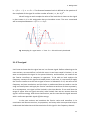
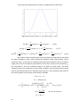
2.7 Digital filters
Digital filters are an essential tool for signal processing. They can be described as linear
shift-invariant systems [2] that let us supress or allow certain frequency intervals. In
the application we use the Kaiser window as the technique to design the filters. We
can see in eq. (2.14) that this window is defined as the quotient of two modified Bessel
functions of zero order of the first kind [6], whose equation we present in eq. (2.15).
( √
⁄(
( )
( )
)
(
( ⁄ )
∑[
]
(
)
)
This technique starts with the design of an ideal filter in the frequency
domain, i.e., with the establishment of the cut-off frequency , through the selection
of the pass-band
and the stop-band
frequencies. In the case of the band-pass
filter, where we have two cut-off frequencies
and
with
, we also
need to choose the central frequency . With these three frequencies we are able to
calculate both cut-off frequencies. The cut-off frequencies are very important because
they are the only variables of the equation of an ideal filter in the time domain, as we
can see in eq. (2.16) for the ideal low-pass filter and in eq. (2.17) and eq. (2.18) for the
ideal high-pass and band-pass filters, respectively. Unfortunately, this equation is
infinite, and therefore, we need to cut it with a window, specifically, the Kaiser
window.
29
Interactive Spectral Manipulation of Music on Mobile Devices in Real-Time
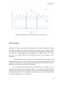
Fig. 13 Kaiser window with
(
(
(
)
)
(
(
points and
)
)
(
(
)
(
)
)
.
(
)
(
)
)
(
)
(
)
(
)
The creation of the window relies on several empirical expressions to provide
the basic variables and , which define the windows shape and duration, with a
numerical value. To be able to compute these empirical expressions we first need to
supply them with the frequency specifications of the filter, namely, the pass-band ,
the stop-band
and the maximum ripple for both of these bands. The basic
variables require the calculation of many other variables. We enumerate them for the
case of the low-pass filter as an example. Note that
is the transition band, and is
the inverse square of the ripple, represented in decibels.
( )
(
{
30
(
)
)
(
)
2. Background
The actual filter that we use results from the multiplication of the ideal filter
by the Kaiser window. To apply it, as we said in Subsection 2.4.2, we need to zero-pad
it in the time domain until it matches the number of samples of the signal
that it
has to multiply in the frequency domain, i.e., samples.
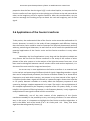
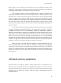
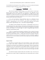
2.8 Frequency interpolation
The coefficients of the spectrum represent only the amplitude of a limited number of
frequencies. In any sound, most of the existing frequencies are not among this limited
group; therefore, most of the times, a frequency of the sound
with maximum local
amplitude does not correspond to the frequency of the coefficient of the spectrum
where we see this maximum. A good way to increase the accuracy in the placement of
these local maxima on the screen is to improve the frequency resolution around these
maxima.
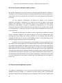
A way to do this is to create a continuous Gaussian curve ( ), where is the
continuous version of , that goes through the amplitude of the coefficient where we
see the maximum
and the amplitude of the two surrounding coefficients,
i.e.,
and
and sample it with a certain interpolation rate . The
position of the maximum of the curve
depends on the value of the amplitude of
the surrounding coefficients, i.e.,
and
. There are two possible
situations: when
, both
and
coincide; if
or
, then
moves towards the coefficient with
the highest amplitude and no longer coincides with
. In the second case, the
frequency corresponding to
is a better approximation of the original frequency
than . In eq. (2.19), we present the equation of the Gaussian curve and in eq. (2.20)
the expression that allows us to find
[11].
( (
( )
(
)
)
(
)
)
(
(
)
)
The fact that we interpolate the spectrum around the local maxima requires us
to do the same for every pair of coefficients in order to keep a constant frequency
interval between all of them. However, in the application, between the coefficients
that are not local maxima or surround them we only interpolate zeroes, which are
31
Interactive Spectral Manipulation of Music on Mobile Devices in Real-Time
disregarded in the spectrum’s visualization process. The resulting frequency resolution
around the local maxima is times lower.
Now that all the theory has been explained, we are prepared to start
introducing more specific content regarding the application. In the next chapter we will
establish the requirements that should be fulfilled and we will explain, in general
terms, the prototype designed to meet them.
32
3
Overview over the Project
We will now put ourselves in the shoes of the users to think about the expectations
they might have regarding the application developed in this thesis. In Section 3.1, we
will combine these expectations and the challenges exposed in Section 1.3, in order to
extract the requirements that we will impose to it. Eventually, we will arrange these
requirements in a priority order.
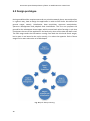
After that, in Section 3.2, we will proceed with a general exposition of the
designed prototype defining the stages that form the whole process of the application
and the detail steps to follow in every stage. Eventually, we will establish the
connections between these steps and the fulfilment of the requirements.
33
Interactive Spectral Manipulation of Music on Mobile Devices in Real-Time
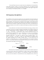
3.1 Requirements engineering
It is very important to establish a set of requirements for the application to fulfil, and it
must be done in an early phase of the project, because they should serve as an
objective for the programming process and as guide for the decision making. As we
said, the aim of this section is to discuss what set of requirements should be
established for the application.
3.1.1 Requirements analysis
We have spotted eleven requirements that might be necessary for the user to be
satisfied with the application. We gather them in four groups that we name precision
requirements, clarity requirements, creativity requirements, and output requirements.
The precision requirements are those that, when met, make the user feel that
he is doing exactly what he intends to, when he intends to. Concerning the application,
it implies an accurate application of any manipulation of the spectrum, and this means
providing the user with as much information as possible about what he wants to do; it
also demands an immediate response in the visual and audio outputs to any
manipulation that comes from the user; and finally, it requires a good synchronization
between both media types.
Precision
requirements
Accuracy
Immediacy
Fig. 14 Precision requirements.
34
Synchronization
3. Overview over the Project
On one hand, the output requirements compel the application to produce an
audio output that can be deemed useful or artistic, i.e., meaningful in some sense. On
the other hand, they demand quality preservation. This implies avoiding any kind of
distortion and generally, maintaining the quality of the original audio file despite the
modifications applied.
Output
requirements
Meaningful
modifications
Quality
preservation
Fig. 15 Output requirements.
The creativity requirements involve the options of sound manipulation that
the application can offer. Specifically, they refer to the variety of effects included, and
the possibility to interact with them once applied as well as to use more than one of
them at the same time.
Creativity
requirements
Variety of
modifications
Interactive
modifications
Coexistence of
modifications
Fig. 16 Creativity requirements.
35
Interactive Spectral Manipulation of Music on Mobile Devices in Real-Time
The clarity requirements demand an application that is intuitive and is easy to
understand and use. This includes a clear disposition of the different elements on the
screen, the differentiation between the representation on the screen of the various
manipulation options and the frequency spectrum, and a way to control the
application that is simple, intuitive, and easy to access.
Clarity
requirements
Disposition of the
elements
Differentiation of
the elements
Easy control
Fig. 17 Clarity requirements.
3.1.2 Priorities
All of these requirements affect different parts of the application and have a different
impact on the application performance. In this section, we assign a priority value to
every requirement. The parameters that we consider for this assignment are three:
i. Their influence on the proper functioning of the application.
ii. Their relevance to the achievement of the overall goals.
iii. Whether they need to be fulfilled entirely or if just a certain degree of
fulfilment is sufficient.
The priority values assigned range from 1 to 3. A priority equal to means
that the requirement must be completely fulfilled for the application to have an
acceptable behaviour. A priority equal to 2 or 3 implies that the requirement should be
met at least in a high or medium degree, respectively. The difference between these
two levels of priority lies, mainly, in the first two parameters. Anyway, their complete
fulfilment is only necessary to achieve the optimal functioning of the application.
36
3. Overview over the Project
Requirement
Precision: Accuracy
Precision: Immediacy
Precision: Synchronization
Output: Meaningful modifications
Output: Quality preservation
Creativity: Variety of the modifications
Creativity: Interactive modifications
Creativity: Coexistence of modifications
Clarity: Disposition of the elements
Clarity: Differentiation of the elements
Clarity: Easy control
Priority
2
1
1
3
1
3
1
2
2
2
2
Table 2 Priorities of the requirements.
The fact that the manipulation of the spectrum is applied in real-time gives
the precision in the time domain great importance. We cannot allow a perceptible
delay between the instant when the user wants to apply the manipulation and the
instant when it is actually applied. In addition, we must ensure that the spectrum we
see on the screen corresponds to the audio we hear at the output. On the other hand,
the precision in the frequency domain, i.e., to which frequencies we are applying the
modifications, is not as crucial for the performance of the application. However, a high
level of accuracy is needed for the user to feel that he is doing what he intends to.
The visual aspect of the application is very important. It must guarantee that
the user can grasp the details of any situation rapidly, identify the different elements
on the screen, and have easy access to the controls. Even though this is essential for
the optimal performance of the application, it can show acceptable behaviour despite
these requirements not completely being met.
To enhance the creativity of the application, it is important to achieve a
significant variety of manipulation options, but it is not the only way to do it. The
possibility to interact with a manipulation once applied or to use two or more of them
at the same time are alternative ways to strengthen the creative side of the
application. As requirements, these are not vital for the application. However, the third
of the challenges stated in Section 1.3 concerns the creativity, and therefore, we must
give them an according priority value.
One of the most important requirements is the quality preservation of the
original file. It is important to avoid or minimize any possible distortion, noise, etc. that
could stain the sound at the output. In the background stays the achievement of
artistically interesting or useful modifications of the sound.
37
Interactive Spectral Manipulation of Music on Mobile Devices in Real-Time
3.2 Design prototype
Having established the requirements and our priorities towards them, we can describe,
in a generic way, how to design the application in order to fulfil them. We define five
general stages, namely, initialization, data acquisition, spectrum manipulation,
spectrum management and playback and visualization. The first one prepares the
ground for the subsequent three stages, which succeed each other forming a cycle that
constitutes the core of the application and ends only when all the data has been read.
The fifth stage needs the information coming from both the third and fourth stages,
but its pace is not bound to the cycle; actually, it is rather the opposite. Each of these
stages has its own main tasks to be developed.
Fig. 18 Cyclic data processing.
38
3. Overview over the Project
As we have said, the first stage carries out all the preparations that allow the
proper development of the following stages. This includes setting the layout of the
activity; extracting essential parameters from the wave file to initialize views and
objects of various classes; assigning values to different parameters; etc. Its last process
is to trigger both the playback of the audio output and the thread that starts the cycle
formed by the stages two, three and four.
The tasks developed in the second stage are to extract a part of the data of
the wave file and prepare it to become the signal, whose spectrum we want to
manipulate and visualize. Once we have obtained the signal, we need to prepare it to
be transformed with the fast Fourier transform algorithm.
Spectrum
Management
Playback and
Visualization
Spectrum
manipulation
Data acquisition
Initialization
The third stage begins with the application of this algorithm, and continues
with the manipulation and the following storage of the resulting spectrum. The fourth
stage starts with the computation of the magnitude of the spectrum and then
proceeds to modify it in order to improve its visualization. As we can see, both stages
overlap in time, but can be conceptually separated: stage three is related to the signal
to be played and stage four to the signal to be visualized.
+
++
++
++
Accuracy
Immediacy
Synchronization
Meaningful modifications
++
Quality preservation
Variety of modifications
Interactive modifications
+
Coexistence of modifications
Disposition of elements
Differentiation of elements
Control
++
++
++
++
++
++
++
+
Table 3 Distribution of the requirements by stages. The symbol “+ +” means that the
requirement is mainly fulfilled in that stage, and the symbol “+” means that only some details
of that requirement are met in that stage.
39
Interactive Spectral Manipulation of Music on Mobile Devices in Real-Time
As we said, the last stage works independently from the other four, but
requires all the data that we store in stages three and four. It basically plays the audio
output and synchronizes it with the spectrum visualization.
Table 3 shows which stages are involved in the fulfilment of the different
requirements. On one hand, we can see that all requirements related to the
modifications and their correct application and control, are dealt with, mainly, in stage
three. This includes the need for a high level of accuracy in and control over the
application of the manipulations. Only the coexistence of these modifications, and just
in some cases, demands the preparation of the signal in stage two. On the other hand,
the demand for immediacy in the response to the user actions and the synchronization
between the audio output and the visualization of its spectrum falls into stage five,
even though the storage of both media types is done in stages three and four.
Finally, we observe that stage one is responsible for the disposition and
differentiation of the elements on the screen as it is where we set the contents of the
view of the activity, and that the task of preserving the quality of the original signal is
shared equally between stages two, where the signal must be appropriately prepared,
and three, where it must be carefully manipulated.
In the next chapter we will further detail the implementation of the different
parts and features of the application. We will base the structure of the explanation on
the stages defined in this section, even though the content covered will be wider.
40
4
Implementation
Up until now we have generally explained the functioning of the application describing
its various stages and explaining their roles and the relationship between them.
Specifically, in Section 3.2, we defined a cycle for the first three stages that can be
understood as the engine that keeps the application working. It is one of the aims of
this chapter to establish how this cycle fits into the actual code of the application.
Thus, we will thoroughly explain the activity that contains it.
It is important to outline that we will describe only one of the two activities of
the application. This activity is called Cycle activity and we will devote sections 4.1 to
4.5 to explain it. Each one of these sections will take care of the description of one of
the stages described in Section 3.2. We will relate the main tasks that they develop
and explain every step needed to accomplish them. For a visual and more detailed
description of the tasks that are carried out in each stage, see Appendix A.
The other – not described – activity basically looks for the wave files available
and shows them on the screen in the form of buttons. When one of these buttons is
clicked, the Cycle activity triggers. We deem that this brief description is enough for
this activity; hence we will not assign a section to it.
Before we start relating the contents of this chapter, we need to do a brief
clarification about the name that we give to the data that we manipulate during the
different processes that form the application. This name changes according to the
phase in which the data is. Once extracted from the wave file, the data becomes the
signal that we transform to the frequency domain to manipulate its spectrum
coefficients. After the modifications we inverse-transform the signal and it becomes
the output signal that is stored in a buffer for playback.
41
Interactive Spectral Manipulation of Music on Mobile Devices in Real-Time
4.1 Stage 1: initialization
As we have said, the processes that take place during the initialization stage lay
the foundations on which the rest of the application is built and allow its proper
functioning in every stage. Specifically, the tasks that this stage accomplishes are the
following:
1. Establishes a pre-programmed xml layout as the content to be visualized for the
duration of the cycle activity. This layout dictates the distribution of the
elements on the screen. Additionally, we place these elements inside objects to
be able to interact with them.
2. Creates a stream of bytes that is bound to the wave file. Through this stream
we can read its contents and handle it much easier, avoiding the memory
problems that can derive from interacting with such big files.
3. Extracts essential parameters for the initialization process from the header of
the wave file. In Subsection 4.3.1, we describe these parameters.
4. Initializes the necessary classes, arrays, variables and other parameters.
5. States the disposition of the buttons of the manipulation menu through a preprogrammed xml menu and handles their call-backs. Additionally, it establishes
how these buttons interact with the class responsible for the application of the
manipulations.
6. Sets the method that informs the application every time the user performs an
action.
7. Prepares the method that controls the seek bar.
8. Starts the playback and triggers the thread that contains the cycle of stages.
The layout of the activity contains a number of views. All of them are always
there, but some of them are not visible the entire time. There are some views that
belong to a certain manipulation, i.e., they show only information about that
manipulation, and are only visible when the manipulation is being applied. We refer to
these views in Subsection 4.3.3, where we describe each kind of manipulation; in this
section we only describe the elements that are not related to any manipulation.
42
4. Implementation
Fig. 19 Basic layout of the application.
As we can see in Fig. 19, there are only four different groups of elements in the
screen. With (1) we refer to the red line that represents the spectrum of the signal.
The specificities of this representation are explained in Section 4.5; (2) is attached to
the manipulation menu that requires a more thorough explanation, which we provide
in Subsection 4.4.2; (3) includes various text views that show information such as the
frequency or amplitude corresponding to the last position of our finger on the screen,
the amplitude of the filters of the equalizer, etc., as well as the frequency and
amplitude scales. These scales are also detailed in Section 4.5; (4) points at a seek bar
that allows us to freely move to any point of the wave file, to have an approximate
idea of its total duration and to know our current position in it. Additionally, when we
place a finger on the screen, two yellow lines appear that cross in that same position.
One of the most important tasks developed in this stage is the obtaining of
some essential parameters for the initialization of every object. A wave file is divided
into two main parts: the header, which takes up 44 bytes [10], and the data. The
header of a wave file contains a lot of information about the data that comes after it.
However, of all this information we are only interested in five parameters.
1. Format: it refers to the way in which the analogue signal has been digitized and
stored in the file. The most usual format and therefore, the one that we use is
the pulse code modulation, as we said in Section 2.1.
43
Interactive Spectral Manipulation of Music on Mobile Devices in Real-Time
2. Number of channels: depending on this parameter, the data inside the wave
file is played as mono or as stereo. The application only admits wave files
defined as mono.
3. Sampling rate: the number of samples that we take of the analogue signal every
second.
4. Bits per sample: the number of bits that we use to represent the value of every
sample.
5. Size of the data: the number of bytes that form the data of the wave file. The
bytes corresponding to the header are not included.
In order for the application to have access to these parameters when needed,
we must store them. To do this, we have to create a stream of bytes that allows us to
read the information inside the wave file, and we must go through the content of the
header discarding the information that is irrelevant to the application and storing the
value of the parameters mentioned above. Finally, we have to check if these values are
among the ones accepted by the application. If they are not, the activity finishes
promptly.
4.2 Stage 2: data acquisition
This stage is basically responsible for the extraction and preparation of the data
contained in the wave file that ultimately constitutes the signal we want to
manipulate, store and play in the following stages.
In Section 2.4.2, as we were describing the time and frequency resolutions, we
mentioned the fact that the application cuts the whole data into smaller parts in order
to achieve an agreement between both resolutions. The parameter that establishes
the maximum number of samples that we can extract in every loop is called capture
rate. In case we are applying certain manipulations, the number of samples extracted
can be lower than the value of this parameter.
In Chapter 2 we already introduced some limitations to the possible values of
the capture rate. Specifically, we explained that the fact that we use a fast Fourier
transform algorithm demands it to be a power of two. The value required must be low
enough to have a time resolution that allows the application to track most of the
changes of the music such as fast notes or silences; and at the same time it must be
44
4. Implementation
high enough to have a frequency resolution that lets us distinguish between close
notes. The value that we consider the best for both the frequency and the time
resolutions is 4096 samples. This value was found heuristically.
The spectrum analysis is closely related with the usage of windows. The
application of windows other than the rectangular, which is always implicit in a data
extraction such as the one we do, brings many benefits but also some disadvantages
[16]. For instance, they allow the reduction of the impact of the side lobes or the
spectral leakage, which are high for the rectangle window, but increase the width of
the main lobe. There is also the possibility to remove them if they fulfil the perfect
reconstruction condition [12] in case we want to recover the original signal after the
spectral analysis.
In our case, the fact that we not only analyse the spectrum but also manipulate
it makes it impossible to apply the window in the time domain. That is why, if we want
to apply one, we must do it in the frequency domain as explained in Chapter 2.
Whether we should apply a window or not depends only on the improvements that we
might observe in the final representation of the spectrum as it does not bring any
other issue. We have tried the Hanning, the Hamming and the 5-terms Blackman
windows [15], and we consider that neither of them improves the visualization of the
spectrum. The growth of the main lobe is the main reason for discarding the usage of
windows as we want to be able to distinguish between close notes.
Once the data is extracted, we must subject it to some operations for it to
become the signal that we want to apply the fast Fourier transform to. This algorithm
works with arrays of doubles as data type because of the precision that the decimals
provide. For proper conversion from bytes to doubles we must pay attention to the
endianness of the data, and to the bits per sample of the wave file to avoid breaking
the samples up.
4.3 Stage 3: spectrum manipulation
When we reach this stage, the signal is already prepared for the computation of its
spectrum, and to endure any of the manipulations available. This section aims to
describe the details of the transformation and inverse transformation processes and to
examine how we apply and interact with the various manipulations that the
application offers.
45
Interactive Spectral Manipulation of Music on Mobile Devices in Real-Time
4.3.1 Fast Fourier transform and its inverse
We already explained how the fast Fourier transform algorithm works in Chapter 2.
Therefore, in this subsection we focus on the particularities of the way this algorithm is
used for both ways of the transform in the specific case of the application developed in
this thesis.
For the spectrum computation, we outline the usage of the symmetry
properties, described in Subsection 2.4.2, that the fact that the signal is real-valued
implies. The symmetry of the spectrum allows us to compute the fast Fourier
transform of two signals at a time, as explained in Subsection 2.5.1. This almost
reduces the execution time of the fast Fourier transform process to 50% and its impact
on the application is decisive to be able to apply heavy manipulations such as very
restrictive filters.
The same way we prepare the data to create a signal that is suitable for the fast
Fourier transform algorithm, we need to adapt the array that contains the signal
resulting from the inverse fast Fourier transform for its playback. We do this by
changing the data type of this array from double to byte or short depending on the
bytes per sample parameter of the current wave file.
However, due to the manipulation of the spectrum, we cannot guarantee that
the values of the output signal are still inside the range of the byte or short data types.
Any sample that exceeds the highest value of this range is cut to this same value,
producing a saturation effect in the output signal. To avoid this, before changing the
data type of the array we need to normalize it to the highest value of the range of the
new data type. After that, we place the signal in the buffer where it waits to be played.
This buffer has a limited size, and when it is full and the application wants to write in it,
the application becomes blocked. This could be interpreted as undesired, but actually
it is very important for the proper functioning of the application as we explain in
Section 4.5.
4.3.2 Spectrum manipulation system
The spectrum manipulation is one of the most crucial steps of the application and
probably the most complex. It is important to note that this step is automatically
skipped as long as we are not applying any manipulation. Once we click a button from
46
4. Implementation
the manipulation menu other than the reset button, the application starts checking
which manipulations are active every time it reaches this step of the cycle and apply
them to the spectrum. If, eventually, we stop every manipulation, for instance, by
means of the reset button, this step will be skipped again in subsequent loops of the
cycle. For an accurate explanation on how to apply, interact with and cancel the
different manipulations, see Appendix B.
Manipulation states
The manipulation menu allows us to control the application, modification and
removal of every manipulation; to manage their coexistence making it possible to work
individually with each one of them avoiding interferences and undesired results; and
to keep track of their state at any moment.
A way to divide the manipulation is by the number of states they can be in. On
one hand, there are the 2-states manipulations. The states are inactive and activeunlocked. For this kind of manipulation, the first click on the button activates it and
either a second click or a click on the reset button deactivates it. Additionally, this type
of manipulation only applies when two conditions are fulfilled: the state has to be set
as active-unlocked and we must be currently interacting with the application, i.e.,
touching the screen.
Fig. 20 Flow of the states for 2-states manipulations. The green arrows represent a
manipulation’s button click and the red ones a click on the reset button.
On the other hand, there are the 3-states manipulations. The states are
inactive, active-unlocked and active-locked. The main difference between the two
types is that the 3-states manipulations, once applied and active, take effect even
when the user is not interacting with the application through the screen. In this case,
the interaction of the user aims to modify the parameters of the manipulation to vary
its effect on the signal. This interaction is only allowed when the state of the
manipulation is set to active-unlocked; if we set it to active-locked, the manipulation
keeps taking effect but we are not able to modify it. This way we can freely touch the
47
Interactive Spectral Manipulation of Music on Mobile Devices in Real-Time
screen to add other manipulations, interact with them or even remove them without
worrying about the ones in the active-locked state.
Fig. 21 Flow of the states for 3-states manipulations. The green arrows represent a
manipulation’s button click and the red ones a click on the reset button.
Mask control system
The key for the implementation of this control system is what we call masks. A
mask is basically an integer that is bound to a manipulation. There is a mask for every
manipulation and the only requirement they must fulfil is to be orthogonal to any
other mask, i.e., the result of their binary multiplication must be equal to zero. The
easiest way to do this is to assign values to these masks that are a power of 2.
Additionally, there are two special masks that do not belong to any manipulation. We
call them mask-unlocked and mask-locked. They start being equal to zero and do not
have to be orthogonal with the other masks.
Every time a manipulation is set to the active-unlocked state we add its mask
value to mask-unlocked. If we remove or lock this manipulation we subtract this value
from this mask. The case of the mask-locked is similar: once a manipulation is set to
the active-locked state, we add its value to this mask and when it is unlocked we
subtract it. This way the value of the mask of a particular manipulation cannot be in
both special masks at the same time.
Note that the multiplication of a specific manipulation’s mask by both of the
special masks allows us to find out the current state of this manipulation. This is the
method that we use every time a signal reaches this stage of the cycle to know what
manipulations it must be subjected to. Additionally, both special masks are used in the
process to set the parameters of the manipulations that need it to make the process
more hermetic.
48
4. Implementation
4.3.3 Types of spectral manipulations
In this subsection we describe details of the different kinds of manipulations that the
application offers such as what is their effect and how we visualize them, which is the
process we must follow to apply them, how can we interact with them once applied,
what information does the application need to handle them, etc.
Synthesizer
The synthesizer allows us to add a new signal to the one that has been
extracted from the wave file and also to modify its spectrum coefficients. The new
signal consists of a fundamental frequency, which compulsorily is among those of the
chromatic musical scale, and its five subsequent harmonics. Initially, all of them have
the same amplitude. However, we can change that in order to modify the sonority of
the added signal.
Most of the frequencies corresponding to the chromatic musical scale are not
represented in the spectrum that we show on the screen; therefore, we cannot add
the new signal through the direct summation of some coefficients to the spectrum.
The process that must be followed consists in the creation of the signal in the time
domain, its transformation to the frequency domain using the fast Fourier transform
and the addition of the result to the spectrum of the extracted signal.
To create the signal in the time domain the first step is to generate as many
samples of the fundamental frequency and every harmonic as necessary for them to
start and finish with a sample of, practically, the same amplitude. Specifically, we stop
the sample generation only when we reach a sample, whose amplitude value is
between the amplitude values of the first sample, i.e., 1, as we create cosines, and the
second sample as shown in Fig. 22. A finite signal is enough because we can infinitely
read it if we use its length as modulo. The errors introduced because of the inaccuracy
of the method are unnoticeable.
Knowing this, we extract from each one of these harmonics the same number
of samples that we are acquiring from the wave file at that moment and sum them
after multiplying them by the coefficient established by the position of our fingers on
the screen. This is the signal we want to transform and then sum to the current
spectrum of the wave file.
49
Interactive Spectral Manipulation of Music on Mobile Devices in Real-Time
Fig. 22 Harmonic creation method. The value of the amplitude of the last sample is between
that of the first and second samples.
The representation in the spectrum of a frequency that is not a multiple of its
frequency resolution has more implications. Specifically, this representation does not
result in a single line but a bunch of them in an attempt to achieve the best
approximation. In consequence, even though initially the amplitude of every harmonic
is the same, we do not see six equally long and equally spaced lines but something
more complex.
This manipulation has only two states: active and inactive. Once we click the
button on the manipulation menu, the manipulation is set to active and the screen
responds to our actions. The first finger we place on the screen establishes the
fundamental frequency and the general amplitude of the signal added. Each
subsequent finger modifies the amplitude of the next harmonic. If we click the button
again or use the reset button, the state is set to inactive.
There is no exclusive view for this manipulation. Its results are summed to the
spectrum of the signal extracted from the wave file and, in consequence, they appear
in the same view.
Filter
One of the most important tools of signal processing is the filter, and in this
application we use them as well. Specifically, we have access to low, high and bandpass filters. For any filter we can define its pass, transition and attenuation bands by
setting the pass and attenuation frequencies and also, in the case of the pass-band
filters, the central frequency. The attenuation in these frequencies, as well as the
amplitude of the filter, is out of the user’s control.
50
4. Implementation
As we said, in the case of a band-pass filter, we must provide three parameters
through our interaction with the screen: the central, the pass and the attenuation
frequencies. For the first parameter it is mandatory to drag one finger over the screen
to the desired frequency because this movement is the one that differentiates a passband filter from a high or low-pass filter. For the other two parameters only a tap on
the screen is required, but we must bear in mind that the attenuation frequency must
be higher than the pass frequency, and that both of them must be higher than the
central frequency. Otherwise, the filter does not appear and the process must be
started again.
For the high and low-pass filters we must tap one time on the screen to let the
application know that we do not want a pass-band filter, and then tap two more times
to set the pass frequency and the attenuation frequency. We assign the values to the
frequencies always in this order. Depending on which of them is higher, we obtain a
high or a low-pass filter.
We explained in Section 2.4.2, that to properly filter the signal we have to
prepare it with the zero-padding technique before we transform it, and also to take
care of the overlap of the result of the inverse transform. To know how many zeroes
we have to insert in the signal we need the filter to be able to tell us its order. We
must take into account that not only the filter manipulation uses filters, also the
equalizer does. Therefore, every time that a loop of the cycle starts, we ask the
manipulations that use filters and that are active at the moment for the order of their
filters and take the biggest order to apply the zero-padding. We use the same value to
solve the problem of the overlapping.
Fig. 23 Example of the filter manipulation.
51
Interactive Spectral Manipulation of Music on Mobile Devices in Real-Time
Only if the manipulation’s state is set to active-unlocked, we can interact with
the filter. To do this we just need to do the same process that we did to apply it. When
we click the button again, the state changes to active-locked and the filter becomes
immune to any interaction coming from us and maintains its effect.
Unlike the synthesizer, this manipulation has its own view. As we can see in Fig.
22, it takes up the same space as the view for the coefficients of the spectrum and
contains the shape of the magnitude of the frequency response of the filter painted
with a green line. Note that this shape is represented linearly in the amplitude axis and
logarithmically in the frequency axis; therefore, the values in decibels written on the
screen do not apply to it. Additionally, during the application and as long as the filter is
active, we can see information about it in the top of the screen.
Equalizer
Even though this manipulation is designed to allow the user to subtly change
the sonority of the signal by emphasizing certain frequency intervals and mitigating
others, it is possible for the equalizer to change the sound significantly and in some
interesting ways. This can be achieved with a bank of 10 filters that cover the entire
spectrum.
Fig. 24 Example of the equalizer manipulation.
52
4. Implementation
To apply the equalizer we just need to click on the manipulation menu and then
tap on the screen. After this, in the screen appear ten bars. The bars show the current
amplitude of each filter and, by tapping on the screen, we can modify them. All these
bars are contained in the equalizer’s own view. Additionally, this manipulation uses a
text view where we can see the current amplitude of the last filter that we modified. If
we click the button again, setting the state of the equalizer to the active-locked, and
tap the screen, the equalization keeps taking effect but we can no longer see the bars.
The range of the amplitude of the filters goes from 0 to 2 and each one of them
affects exactly the frequency interval that is under the corresponding rectangle and
that coincides with those established by the standards [19] [20].
Reset
The reset button stops the manipulations. It is especially important for the
manipulations that can be in the active-locked state because it is the only way to
cancel them. Once the button is clicked, the next tap on the screen stops any
manipulation that is active or active-unlocked. The reset has no effect on the
manipulations that are in the state active-locked or that are already inactive. Note that
if there is no manipulation in an active-unlocked state, the reset button does not
respond. This includes the cases when no manipulation is being applied and when all
the manipulations applied are in the active-locked state.
4.4 Stage 4: spectrum management
This stage starts after the application of the fast Fourier transform. It basically
computes the magnitude of half of the spectrum, as it is symmetric and we only
visualize its first half, and modifies it in order to improve its visualization. Afterwards, it
stores the result of these modifications in an array list where it waits to be called when
the corresponding output signal is being played.
The first step is to apply the interpolation technique explained in Chapter 2.
This greatly improves the frequency resolution of the maxima and also provides a
pleasant shape that improves the visualization especially for the low frequencies up to
300 Hz. Due to the way we visualize the spectrum, which is explained in the next
section, the benefits of this technique for higher frequencies are too low and the
computation effort is too high. Thus, we only apply it to the low frequencies. To do it
53
Interactive Spectral Manipulation of Music on Mobile Devices in Real-Time
we need to identify, beforehand, all the local maxima of the spectrum and space every
coefficient a number of samples equal to the interpolation rate, which is set to 8. This
way we are able to fit the sampled Gaussian curves in every maximum.
The last step before storing the spectrum is to apply the loudness contour as it
is defined in [17]. This helps to make the spectrum more coherent with the sound that
we hear. After this process, the spectrum is ready for its visualization. In the next
section we specify the kind of visualization we use and how it synchronizes with the
playback of the corresponding output signal.
4.5 Stage 5: playback and visualization
The fifth stage of the application aims to play the output signals and to show the
magnitude of the spectrum on the screen in a synchronized way. In this section we
give some details of both processes and eventually explain how the application
achieves their synchronization.
As the output signals must be played at the appropriate rate, stage five has its
own rhythm. Additionally, as we introduced in Section 4.3.1, it has the capacity to
block the cycle of the previous three stages when the buffer where the output signal is
stored is full. This blocking works in our favour because it prevents large accumulations
of manipulated signals in the output that would result in a long delay between the
instant when we apply the manipulation and the instant when the results would be
heard and also visualized on the screen.
The secret of the synchronization between the output signal and the spectrum
visualization is the possibility to receive a notification when the application has played
a certain number of samples. We have to set the notification period to be equal to the
number of samples that we are currently extracting in every loop and with every
notification release one of the arrays containing the magnitude of the spectrum and
show it on the screen.
When we want to change the number of samples extracted, for instance,
because we apply a filter, we also have to change the notification period. However, we
cannot do this immediately because there are already some arrays in the list of the
spectrum magnitudes that must still be called with the previous period. We have to
make sure they have all been shown before changing the notification period.
54
4. Implementation
Regarding the visualization of the spectrum, the coefficients are organized on
the screen by octaves starting at 20 Hz and ending at 20 kHz [18] and a red line unites
the amplitude value in decibels of each of them with the next one. The values of the
frequency scale correspond to those specified in the standards [19] [20]. The values for
the amplitude start at 0 dBFS and go down to a value that includes the lowest possible
amplitude value for the bits per sample of the wave file. Despite that, the coefficients
of the spectrum might take values whose amplitudes in dBFS are much lower. Then,
we use eq. (4.1) to assign a position on the screen, i.e., the
pixel column, to each
frequency coefficient.
(
)(
)(
)
(
)
In the next chapter, we will evaluate the implementation of the application
detailed in this chapter, according to the requirements set in Chapter 3.
55
5
Evaluation
In Chapter 4 we have thoroughly described how we have implemented the application.
Now it is time to assess in which degree this implementation fulfils the requirements
that were established in Chapter 3 and achieves the goals.
We will use two different methods to evaluate the application: an analysis of
technical aspects such as execution times, etc., which will focus on the objective
requirements like the immediacy of the manipulations in the application or the quality
of the output signal; and a survey that will help us collect and organize the sensations,
thoughts and opinions of number of test users. The survey will cover all requirements,
specially focusing on the subjective ones such as those related to the creative
possibilities of the application.
In Section 5.1, we will discuss the most relevant technical aspects and their
relation to the requirements. Section 5.2 will be devoted to explain the particularities
of the test that every candidate will carry out. The questions that we will ask them in
the survey will be explained and referred to the requirements in Section 5.3. Finally,
the result of the evaluation will be shown in Section 5.4.
56
5. Evaluation
5.1 Technical aspects
Capture rate
In Subsection 4.2.2, describing the assignment of a value to the capture rate, we said
that 4096 is the limit that we recommend for this constant. In eq. (5.1) we indicate the
time resolution
of the application using a capture rate
and a sample
⁄ .
rate
⁄
⁄
(
)
Any capture rate value beyond 4096 makes the application start to show
noticeable delays in the spectrum's follow up of the audio output. The reason why is
that any frequency existing in the number of samples captured is shown in the
spectrum for the whole duration of these samples even if it is present only for a
shorter amount of time. This is especially harmful when there are abrupt changes such
as silences that start, for instance, in the middle of the extracted samples or fast notes.
In eq. (5.2), we can see the frequency resolution that corresponds to the
established capture rate. We consider that this resolution value is low enough for the
purposes of the application. However, it can be difficult to distinguish between close
low notes, which differ only by a little more than 1 Hz, but the error is greatly reduced
using the Gaussian interpolation technique [11] explained in Section 2.8 that divides
the resolution by 8 around the local maxima.
⁄
⁄
(
)
Each octave contains a different number of frequency coefficients as the
frequency intervals change from one octave to another. However, the space they
occupy on the screen is the same. The frequency resolution specified in eq. (5.2) is only
valid for those octaves that contain a number of frequencies which is lower than the
number of pixel columns available to them. The other octaves cannot represent all the
coefficients assigned to them and, as a consequence, the frequency resolution
increases. The number of octaves contained in each group depends on the sample rate
of the wave file, but for the lower octaves it is easier to maintain the frequency
resolution unchanged, as their frequency intervals are lower.
As said above, not every frequency coefficient has its own pixel column, as
there are 2048 coefficients to be represented and tablet screens are not usually wide
enough for that. However, there is a frequency for each pixel column even if it does
57
Interactive Spectral Manipulation of Music on Mobile Devices in Real-Time
not coincide with the frequency of any coefficient. In eq. (5.3), we show the formula
we follow to assign a frequency to the pixel column number .
(
)
(
⁄
)
(
)
Note that the frequency interval between low pixel columns is much lower
than for high
pixel columns. Therefore, the accuracy in the application of the
manipulations that we can achieve for low frequencies is higher than for high
frequencies. To assess this accuracy, we must establish the value of the parameters of
eq. (5.3), and define two references. Specifically, we use a sample rate equal to 44100
Hz and a tablet width equal to 1280 pixels.
If we use the frequency interval between notes as a reference for the
assessment, the results are very satisfactory. The lowest interval between pixel
columns is approximately 0.1 Hz at 20 Hz. Around these frequencies the interval
between notes is approximately 1 Hz, i.e., one order of magnitude bigger.
The highest interval between pixel columns is approximately 110 Hz and it
corresponds to the last 2 pixel columns. The frequency corresponding to the last pixel
column is 20480 Hz. The almost inaudible sounds around this frequency are separated
by more than 1000 Hz, an interval, again, an order of magnitude higher than the
frequency interval between pixels.
In [22], it is stated that the frequency resolution of the ear within the octave
from 1000 Hz to 2000 Hz is 3.6 Hz. The highest interval between pixel columns inside
this octave is approximately 10 Hz, i.e., almost three times the ear resolution. With this
second reference, the accuracy of our application cannot be considered as good as
with the first one. Still, we believe that the accuracy requirement has been fulfilled to
a sufficient degree.
Response delay
We define the response delay as the time between a user's action and the
instant when it takes effect. It depends on the size of the buffer and its level of
occupation in the moment of the storage of the output signal. The size is automatically
established by the class responsible for the playback based on the sample rate, the
number of channels and the bits per sample of the wave file. Specifically, the more
samples we need to represent a certain time interval of sound the larger the buffer
becomes.
We obtain the longest response delay when the buffer is full. In this case, the
application has to read a number of samples equal to the whole buffer until it reaches
58
5. Evaluation
the point where the manipulation starts. For a mono wave file sampled at 44100 Hz
and with 16 bits per sample, the usual buffer size is 16384 bits, i.e., 8192 samples. In
eq. (5.4) we calculate the response delay for this case, which is the worst one
considering the kind of wave files that the application accepts.
⁄
(
)
The response delay of the application is obviously in line with the immediacy
requirement. Experiments have shown that a maximum delay of around
is low
enough to consider that this requirement is completely fulfilled taking into account the
reaction times specified in [21].
Loop execution time
There is a limit for the time interval between the instant we write in the buffer
of the audio output and the next writing. This limit is the time spent playing the
samples we have written, and we name it playback time. The playback time depends
on the number of samples that we extract in every loop. Note that the result of eq.
(5.4) is also the playback time when we extract a number of samples equal to the
capture rate.
Basically, we need to give samples to the buffer at a faster pace than the wave
file's sample rate parameter. This is directly related to the quality preservation
requirement. If this simple condition is not fulfilled then the buffer is bound to
eventually become empty. The results of an empty buffer are short but very annoying
silences during the playback. Therefore, it is essential for the quality of the audio
output to prevent the buffer from running out of samples.
The loop execution time is measured as the time necessary to complete a loop
in the case that the buffer is able to accept the samples without blocking it. This
execution time can vary depending on the number of manipulations we apply, but it is
always low enough so that the buffer is never empty.
From Fig. 24 to Fig. 26, we can see three pairs of graphics for three different
situations. For each situation, the first graphic shows the percentage of buffer
occupation for every loop of the cycle and the other presents the loop’s execution
time for every loop with a blue line, the mean of the loop’s execution time with a red
line and the playback time with a green line.
59
Interactive Spectral Manipulation of Music on Mobile Devices in Real-Time
In Situation 1, we are not applying any manipulation to the spectrum and
therefore the number of samples extracted in every loop is equal to the capture rate,
i.e., 4096 samples; the loop’s execution time mean is equal to
; and the
playback time is equal to the result of eq. (5.4). The buffer is completely full the entire
time.
Fig. 25 Situation 1: no manipulation
In Situation 2, we apply a low-pass filter that has a length equal to 396 samples
in the time domain. This means that the number of samples extracted, or the number
of samples we write in the buffer, per loop, is equal to 3700 samples; the loop’s
execution time mean is equal to
; and the playback time is equal
to
. In the buffer’s graphic, we observe a periodic shape. This shape comes
from the difference between the number of samples we write in the buffer every loop,
and the rate at which the samples are extracted from the buffer to be played.
Fig. 26 Situation 2: applying a filter of order N = 396
60
5. Evaluation
The application always extract samples from the buffer in blocks of 1024
samples; therefore, if the rate at which we write the samples to the buffer is not equal
to a multiple of 1024, the buffer gradually empties until, after an extraction, it has free
space equal to two times this last rate and it is completely filled again.
Both the precision of this process and the specific shape of the buffer
occupation graphics depend on the relation between rates and the execution time of
the loop. Situation 1 presents a flat shape because the rates are equal and the loop’s
execution time never comes near the playback time. Therefore, every time the
application extracts samples from the buffer to play them, the buffer is automatically
completely refilled.
Fig. 27 Situation 3: applying filter and equalizer. Also synthesizer from around loop number 20
onwards.
In the Fig. 26 the loop’s execution time surpasses the playback time in many
occasions and the rates do not coincide. The result is an irregular shape with
minimums in the buffer occupation that correspond to the instants when the loop’s
execution time greatly surpasses the playback time. Despite these minimums, the
61
Interactive Spectral Manipulation of Music on Mobile Devices in Real-Time
buffer is never empty. The loop’s execution time mean is
time is
.
, and the playback
As we can see, even in the most demanding situation, the buffer is never
empty. Therefore, we can assume that the quality preservation requirement is fulfilled.
5.2 User feedback
The user evaluation was done face-to-face with a total of 5 candidates, which
had to be music-affine. We provided them the tablet with the application containing 4
songs, each one of them representing a different music style.
S1. Electronic: Alive, by OVERWERK.
S2. Hard Rock: Dream Catcher, by Witchcraft.
S3. Hip hop: Mark, by Shahmen.
S4. Jazz-metal fusion: Hilasterion, by Merkabah.
The method used to test the application is a straightforward semi-structured
interview. We let the candidates know the purpose of the application and, while using
it, we gradually introduce every detail until the candidates know how it works and can
start using it on their own. The candidates listen to every song and try every
manipulation. They can ask as many questions as they want. When they are done, we
interview them as explained in the next section. Additionally, we let them express their
ideas on the improvement possibilities of the application, which we can later add to
the future work section.
5.3 Survey questions
After the test is done we ask the candidates to answer a survey in order to obtain
valuable information for the assessment of the application. The questions included in
this survey are related to one or more of the requirements stated in Chapter 3, so that
we can better evaluate them. The candidates answer each question with a value
62
5. Evaluation
between 0 and 10, where 0 and 10 are the worst and the best result, respectively. In
questions Q6 and Q12 the candidates must rate all the manipulations and all the songs
available, respectively.
Q1.
Do you think that the application is intuitive and easy to control?
Q2.
Do you consider that the information obtained through the screen is
understandable?
Q3.
Do you think that the provided manipulations allow you to use the application
in a creative way?
Q4.
Do you consider the degree of interaction with the manipulation satisfactory?
Q5.
Do you think that the fact that two or more manipulations can coexist is useful?
Q6.
Please, taking into account the results of the three last questions, rate every
manipulation according to your satisfaction.
Q7.
Did you feel any response delay in the application of the different
manipulations?
Q8.
Did you feel that you could apply the manipulations where you wanted to?
Q9.
Do you think that the frequency spectrum moves according to the sound you
hear?
Q10.
Do you think that the different manipulations allowed you to obtain an
artistically significant result?
Q11.
How do you value the quality of the generated sound?
Q12.
Please, rate the performance of the application in every song.
Q1 is related to the requirement for intuitivity and an easy control of the
application. Q2 contains the requirements regarding the disposition and differentiation
of the various elements that appear on the screen. From Q3 to Q5 we evaluate the
creativity requirements. In Q6 we ask the candidate to rate each manipulation. Q7 and
Q8 refer to the immediacy and accuracy requirements. Q9 answers the
synchronization requirement. Q10 and Q11 are related to the output requirements
and, finally, Q12 tries to figure out if there is a difference in the performance of the
application for different kinds of music.
63
Interactive Spectral Manipulation of Music on Mobile Devices in Real-Time
5.4 Survey results
In section 5.1, we discussed several technical aspects that already gave us an indication
about the degree of fulfilment of some requirements. This section aims to finish the
assessment of every requirement stated in Chapter 3 through the comments and
opinions about the application that the users provided us and using the mean of the
results of the survey as a numerical backup.
In every test we have noticed that it is difficult for the candidate to know how
to start using the application. They instinctively click the buttons in the manipulation
menu and tap the screen but not in an order that would produce a satisfactory result.
Despite that, generally, only a short explanation about the application of the
manipulations is necessary to see a great improvement in the performance of the
candidates. We consider that the survey results for question one in Fig. 27, reflect a
mean value between a first impression of helplessness in front of the application and a
learning curve that increases rapidly.
Clarity requirements' questions
10
9
8
7
6
5
4
3
2
1
0
Q1
Q2
Fig. 28 Survey results: questions 1 and 2.
The results for question two are much more satisfactory, as the candidates
define the disposition of the elements on the screen as simple and clear, and find the
colour differentiation between manipulation and the general presentation to be
pleasant. However, some of the candidates mention a lack of information while
applying the synthesizer manipulation or regarding the duration and current time of
the song.
64
5. Evaluation
The aspect which the candidates have been more critical with is the capacity
of the application to enhance the creativity of the user. Even though some of them
admit that with more practice probably their performance would improve, all of them
point to a limited variety of manipulation possibilities as the cause. However, as we
can see in Fig. 28, the candidates appreciate other concepts that can contribute to the
creative aspect of the application, such as the interaction with a manipulation once
applied and the possibility to combine them. Furthermore, when asked about the
quality of each manipulation, the candidates give the filter and the equalizer a score
between 8 and 9 points and 6 points to the synthesizer, as seen in Fig. 29.
Creativity requirements' questions
10
9
8
7
6
5
4
3
2
1
0
Q3
Q4
Q5
Fig. 29 Survey results: questions 3, 4 and 5.
Evaluation of the manipulations
10
9
8
7
6
5
4
3
2
1
0
Q6.Synth
Q6.Filter
Q6.Equal
Fig. 30 Survey results: questions 6.
65
Interactive Spectral Manipulation of Music on Mobile Devices in Real-Time
All the candidates agree on the fact that the delay in the response of the
application to the users actions is low enough; that the accuracy with which the user
can apply the manipulations is satisfactory and the synchronization between the audio
output and visualization of the frequency spectrum is very precise. One of them
underlined the capacity of the frequency spectrum to follow fast changes in the songs
and to distinguish between close notes.
Precision requirements' questions
10
9
8
7
6
5
4
3
2
1
0
Q7
Q8
Q9
Fig. 31 Survey results: questions 7, 8 and 9.
Questions Q10 and Q11 focus on the quality of the audio output, but from
two different points of view: the objective analysis, i.e., the absence of noises such as
clicks specially when we apply manipulations; and the subjective analysis, i.e., if the
application is able to produce an audio output that is artistically interesting or
significant.
In Fig. 31, we observe a big difference between the assessment of the quality
from one point of view and the other. As we said before, the candidates complain
about the creative possibilities of the application, i.e., they opine that the application’s
capacity to create an artistically interesting output is improvable. On the contrary, the
objective assessment of the quality is very satisfactory.
In the last question of the survey, we ask the candidates to rate which songs
are more suitable to use the application with. The results in Fig. 32 are quite balanced
with the electronic music in the first place.
66
5. Evaluation
Output requirements' questions
10
9
8
7
6
5
4
3
2
1
0
Q10
Q11
Fig. 32 Survey results: questions 10 and 11.
Evaluation by music styles
10
9
8
7
6
5
4
3
2
1
0
Q12.Elect
Q12.Rock
Q12.Hip-Hop
Q12.Jazz-Metal
Fusion
Fig. 33 Survey results: question 12.
Fig. 33 is the last graphic of this section and shows the average value of the
results of the questions related to the same group of requirements. We use it to derive
some general conclusions about the evaluation done in this section. Additionally, in
Table 4, we present a summary of the fulfilment of each requirement.
We consider that we have achieved remarkable results concerning the
technical performance of the application. The aspects described in Section 5.1 and the
assessment of the candidates of all the precision requirements and the quality
preservation requirement back this appreciation up.
67
Interactive Spectral Manipulation of Music on Mobile Devices in Real-Time
However, we realize that there is still a great margin for improvement
regarding the creative part of the application in at least two different ways: adding
new manipulations and deepening the study of those already implemented. For
instance, if we have included only a very basic version of a synthesizer, it is partly
because of a need for simplification, as each of the manipulations included in the
application could become the main subject of a different thesis.
Regarding the clarity requirements we believe that the results obtained are
acceptable even though we should improve the way the application communicates
with the user in order to make it more intuitive. Additionally, and thinking about the
future, we should probably shift our focus from buttons to a more innovative way to
apply the manipulations such as more complex gestures.
Requirements average
10
8
6
4
2
0
Clarity
Creativity
Precision
Output
Fig. 34 Survey results: requirements average.
Requirement
Accuracy
Immediacy
Synchronization
Meaningful modifications
Quality preservation
Variety of modifications
Interactive modifications
Coexistence of modifications
Disposition of elements
Differentiation of elements
Control
Fulfilment
Accomplished
Accomplished
Accomplished
Unaccomplished
Accomplished
Unaccomplished
Partially accomplished
Accomplished
Accomplished
Accomplished
Partially accomplished
Table 4 Summary of the fulfilment of each requirement.
68
6
Summary and Conclusions
This Thesis has been developed in compliance with the requirements state by
Technische Universität Wien (TU Wien) and Universitat Politècnica de Catalunya (UPC).
We aim to take advantage of the growth of both the electronic music popularity and
the market involving devices such as tablets or smartphones to create a prototype that
sets the groundwork to mix these two rising phenomena. The application developed
allows us to modify a sound file in real-time through the manipulation of its frequency
spectrum on a mobile device.
We have established a list of requirements that the application must fulfil
considering the users expectations. These requirements are divided in four categories:
the precision requirements that are related to the accuracy and immediacy in the
application of the manipulations and also to the synchronization of the audio output
and the spectrum visualization; the output requirements, which compel the application
to produce an artistically meaningful output that maintains the quality of the original
wave file; the creativity requirements that include the necessity for a variety of
manipulations and the possibility to interact with and combine them; and the clarity
requirements, which demand the application to be intuitive and easy to control, and to
have a clear appearance. Finally, we have stated a priority value to every requirement
that, basically, indicates the importance of their fulfilment.
Afterwards, we have introduced the general design of the application. We
define five general stages that have their own main tasks to develop. The stages are:
the initialization stage, where we set the layout of the activity, create the byte stream
that connects the wave file with the application, retrieve important parameters for the
playback, initialize all the necessary objects and start both the playback and the thread
that forms the core of the application; the data acquisition stage that extracts a part of
69
Interactive Spectral Manipulation of Music on Mobile Devices in Real-Time
the data inside the wave file and prepares it to become the signal that is later
transformed to the frequency domain; the spectrum manipulation stage, which
transforms and inverse-transforms this signal using the fast Fourier transform and
manipulate its spectrum in between; the spectrum management stage that computes
the magnitude of the spectrum and prepares it for visualization; and the playback and
visualization stage, which manages and synchronizes both the audio output and the
spectrum visualization. Eventually, we have specified which requirements are fulfilled
in every stage.
This design prototype has served as an introduction for the further
explanation of the entire contents of the application’s main activity: the Cycle activity.
We have split the description into five sections, one for each stage, and detailed every
step. Additionally, we have provided flow graphs of the stages that visually summarize
their content and help to understand the chain of processes that the application
follows.
We used two methods to evaluate the project: firstly, we have studied and
assessed some technical aspects connected to specific requirements using existing
references, such as the human response time or the ear frequency resolution, when
needed. Secondly, we have asked music-affine test users to test the application and,
afterwards, to answer a survey, with questions related to the requirements, and give
us ideas for further development.
The results of the evaluation of the application are, in general, satisfactory. On
one hand we must emphasize the amply accomplishment of the first challenge stated
in Section 1.3 that was related to the technical performance of the application. On the
other hand we must admit that there is still a lot of work to do in the aspects related to
the creativity and the intuitivity of the application. Nevertheless, we consider that the
work done sets a solid groundwork for future development. We identify four main
improvement paths for the application:
1. Playback control.
2. Formats.
3. Manipulations.
4. Spectrum’s visualization.
Right now we can freely navigate through the song and find the spots we may
want to apply some modifications to or just hear again. Despite that, the precision to
find the right place, especially for long songs, is very low. In this sense we should let
70
6. Summary and Conclusions
the user know the position in time of the song. Additionally, we should add a way for
the user to pause and resume the song at will.
One of the most important improvements that we can think of is to increase
the variety of files that the application can play. We believe that the application should
be able to play all kinds of wave files regardless of the bits per sample or channels they
use, and also other formats of sound files such as mp3, etc.
A revision and improvement of the existing manipulations and the addition of
new ones is essential to keep this project alive. For instance, regarding the synthesizer,
a precise study on how to create sounds could be made in order to make them more
complex and appealing. It could also be a good idea to invest time on the improvement
of the programming of its application through the screen to make it more similar to an
actual instrument. We could add more possibilities in the definition of the parameters
of a filter; extend the bank of filters of the equalizer and their range of amplitudes;
reconsider several aspects of the modulation manipulation such as its utility or
application method, etc.
Eventually, even though we think that the current visualization of the
spectrum is acceptable, there are possibilities to improve it such as the use of
overlapping windows in the extraction of the data. This would result in the addition of
intermediate frequency spectrums that would make its movement smoother. In a
more artistic sense, we could get rid of the straight lines that appear in the low
frequencies and, somehow, try to make the visualization more colourful.
If we can keep this project alive and in constant development, it surely will
end up being an appealing product for those that enjoy the mixture of music and
technology.
71
A
Flow Graphs of the Stages
In this appendix, we present four flow graphs corresponding to stage one, stage two,
stage three and four, and stage five. With them, we aim to complement, in a visual
way, the explanations given in Chapters 3 and 4 about these stages, and to clarify
which is the path that the application follows during its execution.
72
A. Flow Graphs of the Stages
Stage 1: initialization
Fig. 35 Initialization stage’s flow graph.
73
Interactive Spectral Manipulation of Music on Mobile Devices in Real-Time
Stage 2: data acquisition
Fig. 36 Data acquisition stage’s flow graph
74
A. Flow Graphs of the Stages
Stage 3 and 4: spectrum manipulation and spectrum management
Fig. 37 Spectrum manipulation and spectrum management stages’ flow graph.
75
Interactive Spectral Manipulation of Music on Mobile Devices in Real-Time
Stage 5: playback and visualization
Fig. 38 Playback and visualization stage’s flow graph
76
B
Manipulations Manual
In this annex, we summarize the sequence of actions that the user has to take to apply
the different manipulations, interact with them and cancel them in a way similar to
that of a manual.
77
Interactive Spectral Manipulation of Music on Mobile Devices in Real-Time
B.1 Application
Synthesizer
I.
Press the manipulation menu button “SYNTH” to set its state to active-unlocked
“SYNTH: U”.
Filter
I.
Press the manipulation menu button “FILTER” to set its state to active-unlocked
“FILTER: U”.
II.
For a low/high-pass filter tap the screen once.
a. Tap or drag your finger to the desired frequency to fix the pass
frequency.
b. Tap or drag your finger again to the desired frequency to fix the
attenuation frequency.
c. If the pass frequency is lower than the attenuation frequency we obtain
a low-pass filter. Otherwise, we obtain a high-pass filter.
III.
For a band-pass filter drag a finger to the desired frequency to fix the central
frequency.
a. Tap or drag your finger to the desired frequency to fix the pass
frequency. It must be higher than the central frequency.
b. Tap or drag your finger again to the desired frequency to fix the
attenuation frequency. It must be higher than the pass frequency.
c. If the conditions about the frequency values are not met, the filter does
not appear and we have to start from I.
Equalizer
I.
Press the manipulation menu button “EQUAL” to set its state to activeunlocked “EQUAL: U”.
II.
Tap the screen for the equalizing bars to appear.
78
B. Manipulation’s Manual
B.2 Interaction
Synthesizer
I.
Tap with one finger to produce a note and its subsequent five harmonics.
II.
Drag your finger horizontally to change the note and its harmonics.
III.
Drag your finger vertically to change the note’s general volume
IV.
Place one more finger to modify the amplitude of the first harmonic.
Subsequent fingers modify subsequent harmonics. This way we can shape our
waveform.
Filter
I.
For low/high-pass filters:
a. Tap or drag your finger to the desired frequency to fix the pass
frequency.
b. Tap or drag your finger again to the desired frequency to fix the
attenuation frequency.
c. If the pass frequency is lower than the attenuation frequency we obtain
a low-pass filter. Otherwise, we obtain a high-pass filter.
II.
For band-pass filters:
a. Tap or drag your finger to the desired frequency to fix the central
frequency.
b. Tap or drag your finger to the desired frequency to fix the pass
frequency. It must be higher than the central frequency.
c. Tap or drag your finger to the desired frequency to the attenuation
frequency. It must be higher than the pass frequency.
d. If the conditions about the frequency values are not met, the filter
disappears and we have to apply it again.
III.
Press the manipulation menu button “FILTER: U” to set its state to activelocked “FILTER: L”. Now we can no longer interact with the filter. It keeps taking
effect. Another click sets it again to the active-unlocked state “FILTER: U”.
79
Interactive Spectral Manipulation of Music on Mobile Devices in Real-Time
Equalizer
I.
Tap the screen to change the amplitude of the filters of the equalizer.
II.
Press the manipulation menu button “EQUAL: U” to set its state to activelocked “EQUAL: L”. Now we can no longer interact with the equalizer. The bars
disappear but the equalizer keeps taking effect. Another click sets it again to
the active-unlocked state “FILTER: U” and with one tap the bars appear again.
B.3 Cancellation
Synthesizer
I.
Press the manipulation menu button “SYNTH: U” to set its state to inactive
“SYNTH”.
Filter
I.
Press the manipulation menu button “RESET” while the filter is in the activeunlocked state “FILTER: U” and tap the screen.
Equalizer
I.
80
Press the manipulation menu button “RESET” while the equalizer is in the
active-unlocked state “EQUAL: U” and tap the screen.
Bibliography
[1]
A. V. Oppenheim, Alan S. Willsky, S. Hamid Nawab, (1997). Signals & Systems,
Prentice-Hall, Inc., N. J.
[2]
A. V. Oppenheim, Ronald W. Schafer, (1975). Digital Signal Processing,
Prentice-Hall, Inc., N.J.
[3]
Claude E. Shannon (1998). “Communication in the Presence of Noise”, Proc.
Institute of Radio Engineers, Vol.37, No. 1, pp. 10 - 21, Jan. 1949. Reprint as
classic papers in: Proc. IEEE, Vol. 86, No. 2, pp. 447 - 457, February 1998.
[4]
William H. Press, Saul A. Teukolsky, William T. Vetterling, Brian P. Flannery,
(2002). Numerical recipes in C: the art of scientific computing, Cambridge
University Press, N. Y.
[5]
José A. Soares Augusto, (2011). The Io-sinh function, calculation of Kaiser
windows and design of FIR filters, January 1, 2011. http://goo.gl/8KBALy, last
access: August 16, 2014.
[6]
J.F. Kaiser, (1974). “Nonrecursive Digital Filter Design Using the Io-sinh Window
Function”, Proc. 1974 IEEE Int. Symp. Circuit Theory, pp. 20 - 23.
[7]
Institut de Recherche et Coordination Acoustique/Musique, IRCAM (2011).
AudioSculpt 3.0 User Manual. http://goo.gl/P8OgVj, last access: August 16,
2014.
[8]
Reactable Systems (2011). Reactable Live! Manual. http://goo.gl/RMAee1, last
access: August 16, 2014.
[9]
Thomas Fine (2008). “The Dawn of Commercial Digital Recording”, ARSC
Journal, Vol. 39, No. 1, Spring 2008. http://goo.gl/CKmOq2, last access: August
16, 2014.
81
Interactive Spectral Manipulation of Music on Mobile Devices in Real-Time
[10]
[11]
Centre for Computer Research in Music and Acoustics, CCRMA (2003). Wave
PCM Soundfile Format. http://goo.gl/V9935E, last access: August 16, 2014.
M. Gasior, J.L. Gonzalez, (2004). “Improving FFT Frequency Measurement
Resolution by Parabolic and Gaussian Interpolation”, AB-Note-2004-021 BDI,
CERN, February 2004.
[12]
Ivan W. Selesnick (2009). Short-Time Fourier Transform and Its Inverse, April 14,
2009. http://goo.gl/YLoHXK, last access: August 16, 2014.
[13]
Library of Congress (2010). “Linear Pulse Code Modulated Audio (LPCM)”,
Sustainability for Digital Formats Planning for Library of Congress Collections,
Library of Congress, March 21, 2010. http://goo.gl/1kNOnR, last access: August
16, 2014.
[14]
Nuggehally S. Jayant, Peter Noll (1984). Digital Coding of Waveforms, Prentice
Hall, Inc., Englewood Cliffs, N. J.
[15]
T. L. J. Ferris, A. J. Grant (1992). “Frequency Domain Method for Windowing in
Fourier Analysis”, Electronic Letters, Vol. 28, No. 15, pp. 1440, July 16, 1992.
[16]
Harris. F (1978), “On the use of windows for harmonic analysis with discrete
Fourier transform”, Proc. IEEE, 66, pp. 51 - 83, 1978.
[17]
International Standarization Organization, ISO 226:2003(E): Acoustics - Normal
Equal-Loudness-Level Contours, Geneva, Switzerland.
[18]
Federico Miyara (2004), Ecualizadores, http://goo.gl/whbYsV, last access:
August 16, 2014.
[19]
IEC 61260:1995 Octave-Band and Fractional-Octave-Band Filters.
[20]
IRAM 4081:1977 Filtros de banda de octava, de media octava, de tercio de
octava, destinados al análisis de sonidos y vibraciones.
[21]
Robert J. Kosinski (2013), A Literature Review on Reaction Time, Clemson
University, USA, September 2013, http://goo.gl/sPuJCd, last access: August 16,
2014.
[22]
Harry F. Olson (1967), Music, Physics and Engineering, Dover Publications, pp.
248 - 251.
82