No category

Download Dynamic linker and debugging/tracing interface for HelenOS

Transcript

Charles University in Prague
Faculty of Mathematics and Physics
MASTER THESIS
Jiří Svoboda
Dynamic linker and debugging/tracing
interface for HelenOS
Department of Software Engineering
Supervisor: Mgr. Martin Děcký
Study program: Computer science, Software systems
2
I would like to thank my supervisor Mgr. Martin Děcký for reading through the
preliminary versions of this document, for valuable suggestions and for kind words
of support. I am also indebted to him for introducing me to HelenOS.
I would also like to thank Jakub Jermář for countless hours of discussion, for all
his advice, constant encouragement and for persuading me to ﬁnd better solutions
to problems. I also owe him for implementing VFS just in time for me to use it and
for conceiving HelenOS in the ﬁrst place. Last, but certainly not least, I must thank
Jakub for being a great friend.
Thank you.
I hereby declare that I have written this thesis myself, on my own and solely using
the cited sources. I give permission to loan this document.
Prohlašuji, že jsem svou diplomovou práci napsal samostatně a výhradně s použitím
citovaných pramenů. Souhlasím se zapůjčováním práce.
V Praze dne 11. 12. 2008
Jiří Svoboda
..............
3
4
Contents
Cover Page
1
Contents
List of Tables . . . . . . . . . . . . . . . . . . . . . . . . . . . . . . . . . .
List of Figures . . . . . . . . . . . . . . . . . . . . . . . . . . . . . . . . . .
8
9
9
1 Introduction
1.1 Motivation . . . . . . . . . . . . . . . . . . .
1.2 Goals . . . . . . . . . . . . . . . . . . . . . .
1.3 Getting the Source Code . . . . . . . . . . .
1.4 How to Read This Document . . . . . . . .
1.4.1 Organization of This Document . . .
1.4.2 Conventions Used in This Document
2 HelenOS Overview
2.1 History of SPARTAN and HelenOS . . . . .
2.2 Multiprocessing Support . . . . . . . . . . .
2.2.1 Scheduling . . . . . . . . . . . . . . .
2.2.2 Synchronization . . . . . . . . . . . .
2.3 Memory Management . . . . . . . . . . . . .
2.4 User-Space Tasks . . . . . . . . . . . . . . .
2.4.1 Creation of a Task . . . . . . . . . .
2.4.2 Creating New Tasks from User Space
2.4.3 Identifying Kernel Resources . . . . .
2.5 IPC Subsystem . . . . . . . . . . . . . . . .
2.5.1 Low-Level IPC . . . . . . . . . . . .
2.5.2 System-Call IPC Layer . . . . . . . .
2.5.3 Message Processing . . . . . . . . . .
2.5.4 Asynchronous Library . . . . . . . .
2.5.5 Connections and the Naming Service
2.6 Further Reading . . . . . . . . . . . . . . . .
2.7 SMC Coherency . . . . . . . . . . . . . . . .
2.7.1 Why Self-Modifying Code? . . . . . .
2.7.2 Contemporary Memory Architecture
2.7.3 Coherency Problems . . . . . . . . .
2.7.4 Instruction Memory Barriers . . . . .
2.7.5 SMC Coherency in HelenOS . . . . .
5
.
.
.
.
.
.
.
.
.
.
.
.
.
.
.
.
.
.
.
.
.
.
.
.
.
.
.
.
.
.
.
.
.
.
.
.
.
.
.
.
.
.
.
.
.
.
.
.
.
.
.
.
.
.
.
.
.
.
.
.
.
.
.
.
.
.
.
.
.
.
.
.
.
.
.
.
.
.
.
.
.
.
.
.
.
.
.
.
.
.
.
.
.
.
.
.
.
.
.
.
.
.
.
.
.
.
.
.
.
.
.
.
.
.
.
.
.
.
.
.
.
.
.
.
.
.
.
.
.
.
.
.
.
.
.
.
.
.
.
.
.
.
.
.
.
.
.
.
.
.
.
.
.
.
.
.
.
.
.
.
.
.
.
.
.
.
.
.
.
.
.
.
.
.
.
.
.
.
.
.
.
.
.
.
.
.
.
.
.
.
.
.
.
.
.
.
.
.
.
.
.
.
.
.
.
.
.
.
.
.
.
.
.
.
.
.
.
.
.
.
.
.
.
.
.
.
.
.
.
.
.
.
.
.
.
.
.
.
.
.
.
.
.
.
.
.
.
.
.
.
.
.
.
.
.
.
.
.
.
.
.
.
.
.
.
.
.
.
.
.
.
.
.
.
.
.
.
.
.
.
.
.
.
.
.
.
.
.
.
.
.
.
.
.
.
.
.
.
.
.
.
.
.
.
.
.
.
.
.
.
.
.
.
.
.
.
.
.
.
.
.
.
.
.
.
.
.
.
.
.
.
.
.
.
.
.
.
.
.
.
.
.
.
.
.
.
.
.
.
.
.
.
.
.
.
.
.
.
.
.
.
.
.
.
.
.
.
.
.
.
11
11
11
12
13
13
13
.
.
.
.
.
.
.
.
.
.
.
.
.
.
.
.
.
.
.
.
.
.
15
15
15
15
16
17
17
17
18
18
18
18
19
19
20
21
21
21
21
22
22
23
23
3 Debugging and Tracing Overview
3.1 Bugs and Observability . . . . . . . . . . . .
3.1.1 Hunting Bugs . . . . . . . . . . . . .
3.1.2 Observability . . . . . . . . . . . . .
3.1.3 Impact . . . . . . . . . . . . . . . . .
3.1.4 Common Debugging Methods . . . .
3.1.5 Common Techniques . . . . . . . . .
3.1.6 Debugging Software . . . . . . . . . .
3.1.7 Data for Post-Mortem Analysis . . .
3.1.8 Methods for Static Analysis . . . . .
3.2 Breakpoint Debugging Support in Processors
3.3 Network Packet Analysis . . . . . . . . . . .
.
.
.
.
.
.
.
.
.
.
.
.
.
.
.
.
.
.
.
.
.
.
.
.
.
.
.
.
.
.
.
.
.
.
.
.
.
.
.
.
.
.
.
.
.
.
.
.
.
.
.
.
.
.
.
.
.
.
.
.
.
.
.
.
.
.
.
.
.
.
.
.
.
.
.
.
.
.
.
.
.
.
.
.
.
.
.
.
.
.
.
.
.
.
.
.
.
.
.
27
27
27
27
27
28
28
29
30
30
30
31
4 Debugging and Tracing Design and Implementation
4.1 Design Overview . . . . . . . . . . . . . . . . . . . . .
4.2 Supported Architectures . . . . . . . . . . . . . . . . .
4.3 Udebug Interface . . . . . . . . . . . . . . . . . . . . .
4.3.1 Interface Form . . . . . . . . . . . . . . . . . .
4.3.2 Connecting . . . . . . . . . . . . . . . . . . . .
4.3.3 Debugging Message Format . . . . . . . . . . .
4.3.4 Debugging Methods . . . . . . . . . . . . . . .
4.3.5 Typical Debugging Session . . . . . . . . . . . .
4.3.6 Events . . . . . . . . . . . . . . . . . . . . . . .
4.4 Udebug Implementation . . . . . . . . . . . . . . . . .
4.4.1 Implementation Overview . . . . . . . . . . . .
4.4.2 Suspending and Resuming Threads . . . . . . .
4.4.3 Hooks . . . . . . . . . . . . . . . . . . . . . . .
4.4.4 Task Memory Access . . . . . . . . . . . . . . .
4.4.5 Kbox Thread Beneﬁts . . . . . . . . . . . . . .
4.4.6 Register State Access . . . . . . . . . . . . . . .
4.4.7 Synchronization and State Management . . . .
4.5 System Call/IPC Tracer . . . . . . . . . . . . . . . . .
4.5.1 Overview . . . . . . . . . . . . . . . . . . . . .
4.5.2 End-User Perspective . . . . . . . . . . . . . . .
4.5.3 Under the Hood . . . . . . . . . . . . . . . . . .
4.6 Breakpoint Debugger . . . . . . . . . . . . . . . . . . .
4.6.1 Overview . . . . . . . . . . . . . . . . . . . . .
4.6.2 End-User Perspective . . . . . . . . . . . . . . .
4.6.3 Under the Hood . . . . . . . . . . . . . . . . . .
4.7 Future Work . . . . . . . . . . . . . . . . . . . . . . . .
.
.
.
.
.
.
.
.
.
.
.
.
.
.
.
.
.
.
.
.
.
.
.
.
.
.
.
.
.
.
.
.
.
.
.
.
.
.
.
.
.
.
.
.
.
.
.
.
.
.
.
.
.
.
.
.
.
.
.
.
.
.
.
.
.
.
.
.
.
.
.
.
.
.
.
.
.
.
.
.
.
.
.
.
.
.
.
.
.
.
.
.
.
.
.
.
.
.
.
.
.
.
.
.
.
.
.
.
.
.
.
.
.
.
.
.
.
.
.
.
.
.
.
.
.
.
.
.
.
.
.
.
.
.
.
.
.
.
.
.
.
.
.
.
.
.
.
.
.
.
.
.
.
.
.
.
.
.
.
.
.
.
.
.
.
.
.
.
.
.
.
.
.
.
.
.
.
.
.
.
.
.
.
.
.
.
.
.
.
.
.
.
.
.
.
.
.
.
.
.
.
.
.
.
.
.
.
.
33
33
34
34
34
34
35
35
37
38
39
39
40
43
44
46
46
48
51
51
51
52
53
53
53
54
55
.
.
.
.
.
.
.
57
57
57
57
58
59
59
59
5 Dynamic Linking Overview
5.1 Basic Concepts . . . . . . .
5.1.1 Separate Compilation
5.1.2 Symbols . . . . . . .
5.1.3 Object Files . . . . .
5.1.4 Sections . . . . . . .
5.1.5 Executable Files . .
5.1.6 Loader . . . . . . . .
.
.
.
.
.
.
.
.
.
.
.
.
.
.
.
.
.
.
.
.
.
6
.
.
.
.
.
.
.
.
.
.
.
.
.
.
.
.
.
.
.
.
.
.
.
.
.
.
.
.
.
.
.
.
.
.
.
.
.
.
.
.
.
.
.
.
.
.
.
.
.
.
.
.
.
.
.
.
.
.
.
.
.
.
.
.
.
.
.
.
.
.
.
.
.
.
.
.
.
.
.
.
.
.
.
.
.
.
.
.
.
.
.
.
.
.
.
.
.
.
.
.
.
.
.
.
.
.
.
.
.
.
.
.
.
.
.
.
.
.
.
.
.
.
.
.
.
.
.
.
.
.
.
.
.
.
.
.
.
.
.
.
.
.
.
.
.
.
.
.
.
.
.
.
.
.
.
.
.
.
.
.
.
.
.
.
.
.
.
.
.
.
.
.
.
.
.
.
.
.
.
.
.
.
.
.
.
.
.
.
5.2
5.3
5.4
5.5
5.1.7 Linker . . . . . . . . . . . . . . . . . . .
5.1.8 Libraries . . . . . . . . . . . . . . . . . .
5.1.9 Dynamically-Linked Libraries . . . . . .
5.1.10 Loading a Library at Run Time . . . . .
5.1.11 ELF and the System V ABI . . . . . . .
5.1.12 Library ABI and Versioning . . . . . . .
5.1.13 Thread-Local Storage . . . . . . . . . . .
Executable and Linking Format (ELF) . . . . .
5.2.1 Features . . . . . . . . . . . . . . . . . .
5.2.2 File Structure Overview . . . . . . . . .
5.2.3 ELF Header . . . . . . . . . . . . . . . .
5.2.4 Sections . . . . . . . . . . . . . . . . . .
5.2.5 Segments . . . . . . . . . . . . . . . . .
5.2.6 String Table . . . . . . . . . . . . . . . .
5.2.7 Symbol Table . . . . . . . . . . . . . . .
5.2.8 Relocation Table . . . . . . . . . . . . .
ELF Dynamic Linking . . . . . . . . . . . . . .
5.3.1 Base Address . . . . . . . . . . . . . . .
5.3.2 Program Interpreter . . . . . . . . . . .
5.3.3 Dynamic Section . . . . . . . . . . . . .
5.3.4 Shared Library Dependencies . . . . . .
5.3.5 Global Oﬀset Table . . . . . . . . . . . .
5.3.6 Procedure Linkage Table . . . . . . . . .
5.3.7 Hash Table . . . . . . . . . . . . . . . .
5.3.8 Initialization and Termination Functions
GNU Linker . . . . . . . . . . . . . . . . . . . .
ELF Thread-Local Storage . . . . . . . . . . . .
6 Dynamic Linking Design and Implementation
6.1 Overview . . . . . . . . . . . . . . . . . . . . . .
6.2 Supported Architectures . . . . . . . . . . . . .
6.3 Building . . . . . . . . . . . . . . . . . . . . . .
6.4 Program Loader . . . . . . . . . . . . . . . . . .
6.4.1 Interim Solution . . . . . . . . . . . . . .
6.4.2 Cracking the Chicken and Egg Problem .
6.4.3 Kernel Infrastructure . . . . . . . . . . .
6.4.4 Entry-Point Interface . . . . . . . . . . .
6.4.5 Program Control Block . . . . . . . . . .
6.4.6 IPC Communication Protocol . . . . . .
6.4.7 Library API . . . . . . . . . . . . . . . .
6.4.8 Program Loader Implementation . . . .
6.4.9 SMC Coherency . . . . . . . . . . . . . .
6.5 Dynamic Linker . . . . . . . . . . . . . . . . . .
6.5.1 The Big Picture . . . . . . . . . . . . . .
6.5.2 Design Considerations . . . . . . . . . .
6.5.3 Source Code Structure . . . . . . . . . .
6.5.4 Dynamic Linker Operation in a Nutshell
6.5.5 Building the Shared C Library . . . . . .
6.5.6 Trying out the Dynamic Linker . . . . .
7
.
.
.
.
.
.
.
.
.
.
.
.
.
.
.
.
.
.
.
.
.
.
.
.
.
.
.
.
.
.
.
.
.
.
.
.
.
.
.
.
.
.
.
.
.
.
.
.
.
.
.
.
.
.
.
.
.
.
.
.
.
.
.
.
.
.
.
.
.
.
.
.
.
.
.
.
.
.
.
.
.
.
.
.
.
.
.
.
.
.
.
.
.
.
.
.
.
.
.
.
.
.
.
.
.
.
.
.
.
.
.
.
.
.
.
.
.
.
.
.
.
.
.
.
.
.
.
.
.
.
.
.
.
.
.
.
.
.
.
.
.
.
.
.
.
.
.
.
.
.
.
.
.
.
.
.
.
.
.
.
.
.
.
.
.
.
.
.
.
.
.
.
.
.
.
.
.
.
.
.
.
.
.
.
.
.
.
.
.
.
.
.
.
.
.
.
.
.
.
.
.
.
.
.
.
.
.
.
.
.
.
.
.
.
.
.
.
.
.
.
.
.
.
.
.
.
.
.
.
.
.
.
.
.
.
.
.
.
.
.
.
.
.
.
.
.
.
.
.
.
.
.
.
.
.
.
.
.
.
.
.
.
.
.
.
.
.
.
.
.
.
.
.
.
.
.
.
.
.
.
.
.
.
.
.
.
.
.
.
.
.
.
.
.
.
.
.
.
.
.
.
.
.
.
.
.
.
.
.
.
.
.
.
.
.
.
.
.
.
.
.
.
.
.
.
.
.
.
.
.
.
.
.
.
.
.
.
.
.
.
.
.
.
.
.
.
.
.
.
.
.
.
.
.
.
.
.
.
.
.
.
.
.
.
.
.
.
.
.
.
.
.
.
.
.
.
.
.
.
.
.
.
.
.
.
.
.
.
.
.
.
.
.
.
.
.
.
.
.
.
.
.
.
.
.
.
.
.
.
.
.
.
.
.
.
.
.
.
.
.
.
.
.
.
.
.
.
.
.
.
.
.
.
.
.
.
.
.
.
.
.
.
.
.
.
.
.
.
.
.
.
.
.
.
.
.
.
.
.
.
.
.
.
.
.
.
.
.
.
.
.
.
.
.
.
.
.
.
.
.
.
.
.
.
.
.
.
.
.
.
.
.
.
.
.
.
.
.
.
.
.
.
.
.
.
.
.
.
.
.
.
.
.
.
.
.
.
.
.
.
.
.
.
.
.
.
.
.
.
.
.
.
.
.
.
.
.
.
.
.
.
.
.
.
59
59
60
60
61
61
62
63
63
63
63
63
64
64
65
65
65
65
66
66
66
67
67
68
68
69
69
.
.
.
.
.
.
.
.
.
.
.
.
.
.
.
.
.
.
.
.
71
71
71
71
72
72
72
74
74
75
75
76
77
77
77
77
78
80
82
84
85
6.5.7
Future Work . . . . . . . . . . . . . . . . . . . . . . . . . . . . 85
7 Related Work
7.1 Debugging on UNIX System V . .
7.2 Debugging on Microsoft Windows .
7.3 Dynamic Linking on UNIX Systems
7.4 Dynamic Linking on Windows . . .
7.5 Debugging on Linux and Solaris . .
7.6 QNX Neutrino . . . . . . . . . . .
7.7 OKL4 . . . . . . . . . . . . . . . .
7.8 MINIX . . . . . . . . . . . . . . . .
7.9 GNU Hurd . . . . . . . . . . . . . .
.
.
.
.
.
.
.
.
.
.
.
.
.
.
.
.
.
.
.
.
.
.
.
.
.
.
.
.
.
.
.
.
.
.
.
.
.
.
.
.
.
.
.
.
.
.
.
.
.
.
.
.
.
.
.
.
.
.
.
.
.
.
.
.
.
.
.
.
.
.
.
.
.
.
.
.
.
.
.
.
.
.
.
.
.
.
.
.
.
.
.
.
.
.
.
.
.
.
.
.
.
.
.
.
.
.
.
.
.
.
.
.
.
.
.
.
.
.
.
.
.
.
.
.
.
.
.
.
.
.
.
.
.
.
.
.
.
.
.
.
.
.
.
.
.
.
.
.
.
.
.
.
.
.
.
.
.
.
.
.
.
.
.
.
.
.
.
.
.
.
.
87
87
87
88
88
88
89
89
89
90
8 Conclusion
91
8.1 Achievements . . . . . . . . . . . . . . . . . . . . . . . . . . . . . . . 91
8.2 Contributions . . . . . . . . . . . . . . . . . . . . . . . . . . . . . . . 91
8.3 Perspectives . . . . . . . . . . . . . . . . . . . . . . . . . . . . . . . . 91
Bibliography
93
8
List of Tables
4.1
4.2
4.3
4.4
4.5
Debugging Request Structure . . . .
Debugging Reply Structure . . . . .
Debugging Methods . . . . . . . . . .
Debugging Event Message Structure .
Debugger Commands . . . . . . . . .
.
.
.
.
.
.
.
.
.
.
.
.
.
.
.
.
.
.
.
.
.
.
.
.
.
.
.
.
.
.
.
.
.
.
.
.
.
.
.
.
.
.
.
.
.
.
.
.
.
.
.
.
.
.
.
.
.
.
.
.
.
.
.
.
.
.
.
.
.
.
.
.
.
.
.
.
.
.
.
.
.
.
.
.
.
.
.
.
.
.
35
35
36
38
54
6.1 Loader Low-Level Library API . . . . . . . . . . . . . . . . . . . . . . 76
6.2 Implemented IA-32 Relocation Types . . . . . . . . . . . . . . . . . . 83
6.3 Implemented PowerPC Relocation Types . . . . . . . . . . . . . . . . 83
List of Figures
2.1 IPC Message Processing . . . . . . . . . . . . . . . . . . . . . . . . . 20
4.1 Debugging-Session Management Example . . . . . . . . . . . . . . . . 43
4.2 Debugging State Transitions . . . . . . . . . . . . . . . . . . . . . . . 49
5.1 Thread-Local Storage Data Structures . . . . . . . . . . . . . . . . . 70
6.1 Debugging-Session Management Example . . . . . . . . . . . . . . . . 73
6.2 Task Address-Space Layout with Loader Present . . . . . . . . . . . . 73
6.3 Task Address-Space Layout with Loader and Linker . . . . . . . . . . 80
9
Title: Dynamic linker and debugging/tracing interface for HelenOS
Author: Jiří Svoboda
Department: Department of Software Engineering, MFF UK
Supervisor: Mgr. Martin Děcký
Supervisor’s e-mail address: Martin.Decky@mﬀ.cuni.cz
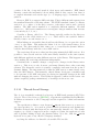
Abstract: HelenOS is an operating system that originated as a software project at
the Faculty of Mathematics and Physics. So far it lacks support for dynamically
linked libraries as well as support for process tracing and debugging.
Dynamically linked libraries enable developing individual parts of large software
systems independently and linking them later together without recompilation. The
linking is carried out at load-time or run-time by the dynamic linker. The linker
must ﬁnd all libraries used by the program, map them into memory and relocate
them. Then it must resolve external (symbolic) references between the program and
libraries.
A debugger and a system-call tracer are essential development tools. They use a
special system interface for their operation enabling them to suspend an application
when certain events occur (such as a breakpoint or a trap). Then they may examine
or change the application’s memory contents and resume its execution.
The main goal of this thesis is to implement support for dynamically linked libraries in HelenOS, namely the dynamic linker, and also a system API for debugging
and tracing processes, including a demo application.
Keywords: dynamically, linked, libraries, debugging, tracing
Název práce: Dynamický linker a rozhraní pro ladění a trasování v HelenOS
Autor: Jiří Svoboda
Katedra (ústav): Katedra softwarového inženýrsví, MFF UK
Vedoucí diplomové práce: Mgr. Martin Děcký
E-mail vedoucího: Martin.Decky@mﬀ.cuni.cz
Abstrakt: HelenOS je operační systém, který vznikl vrámci softwarového projektu
na MFF UK. V systému zatím chybí podpora dynamických knihoven a ladění a
trasování procesů.
Dynamické knihovny umožňují vyvíjet části velkých softwarových systémů odděleně a později je spojit bez nutnosti opakovaného překladu. Toto spojování
provádí dynamický linker a to během zavádění programu, nebo až za běhu. Linker
musí nalézt všechny knihovny vyžadované programem, zavést je do paměti a relokovat je. Potom musí vyřešit externí (symbolické) odkazy mezi programem a jednotlivými knihovnami.
Debugger a trasovač systémových volání patří mezi základní ladicí nástroje. Ke
své činnosti využívají speciální systémové rozhraní, které jim umožňuje pozastavit
aplikaci, když v ní dojde k určitým událostem (např. breakpoint, trap nebo volání
systému). Mohou číst nebo měnit obsah paměti aplikace a opět obnovit její běh.
Hlavním cílem této práce je přidat do systému podporu pro dynamické knihovny,
tedy zejména dynamický linker, a dále systémové rozhraní pro ladění a trasování
procesů s ukázkovou aplikací.
Klíčová slova: dynamické, knihovny, ladění, trasování
10
Chapter 1
Introduction
1.1
Motivation
Operating systems have been around for more than forty years. Today they are
practically omnipresent and indispensable. They are the key piece of ‘glue’ that ties
the hardware, the software and the user together. Owing to the enormous changes
the hardware has undergone in the past decades, there are software developers who
believe it is worth dropping the legacy code completely and starting an operating
system from scratch.
One such project is HelenOS. Building upon the solid base of the SPARTAN
microkernel, the development eﬀorts are now shifting to the userland. To grow
further, the project needs an active community and to gain a wider audience, there
are still technical gaps that need to be ﬁlled.
Until now HelenOS had no support whatsoever for debugging user-space tasks,
which already proved a severe disadvantage. Also, the binary image of the system
was starting to grow at an alarming rate as the standard C library had been linked
again and again into every single binary.
In this thesis we describe the decisions taken during the design and implementation of a debugging/tracing interface and a dynamic linker for the HelenOS operating
system.
1.2
Goals
The aim of this thesis is to explain the design and implementation of HelenOS
debugging, tracing and dynamic linking facilities. The implementation should result
in the following:
• a system interface for building user-space task debuggers and system call tracing programs.
• a simple example of a debugger.
• a simple example of a system call tracer.
• a dynamic linker.
• a shared version of the HelenOS C library.
11
We will particularly emphasize the aspects of the design that bear some relationship to the speciﬁcs of the HelenOS system (mainly its microkernel nature and
its IPC subsystem). We will also discuss the similarities and diﬀerences of similar
facilities in some notable operating systems.
1.3
Getting the Source Code
To obtain the latest source code you can go to the HelenOS project website at
http://www.helenos.org/. This will point you to the Subversion repository which
resides at the URL svn://svn.helenos.org/HelenOS. The repository can also be
browsed on-line at http://trac.helenos.org/trac.fcgi/browser.
The dynamic linking code currently resides in the ‘dynload’ branch. The debugging and tracing implementation can be found in the ‘tracing’ branch. The source
code in both of these branches can only be built for those architectures that are
currently supported (ia32 and ppc32 for dynamic linking and arm32, ia32, mips32
and ppc32 for debugging). The program loader and the tracing part alone are already in the trunk and they can be built for any architecture supported by HelenOS.
The code that constitutes the work on this thesis resides in the following ﬁles and
directories:
Common code for debugging and tracing (both in the trunk and all branches)
kernel/generic/include/udebug
kernel/generic/src/udebug
kernel/generic/src/ipc/kbox.c
uspace/lib/libc/include/udebug.h
uspace/lib/libc/generic/udebug.c
uspace/app/trace
Extra code needed for debugging (only in the ‘tracing’ branch)
kernel/generic/include/mm/as\_debug.h
kernel/generic/src/mm/as\_debug.c
uspace/app/debug
Dynamic linking code (only in the ‘dynload’ branch)
uspace/lib/rtld
uspace/lib/libc/include/dlfcn.h
uspace/lib/libc/generic/dlfcn.c
uspace/lib/libc/shared
uspace/lib/libtest
uspace/app/dload
Program loader (both in the trunk and in all branches)
kernel/generic/include/proc/program.h
kernel/generic/src/proc/program.c
uspace/lib/libc/include/loader
uspace/lib/libc/generic/loader.c
uspace/lib/libc/generic/task.c
uspace/srv/loader
12
If you are unable to ﬁnd these ﬁles, please make sure you are looking in the right
branch. Small changes were made throughout the kernel, but they are too numerous
to list here. The entire history of changes can be found in the log of the HelenOS
source code repository.
1.4
1.4.1
How to Read This Document
Organization of This Document
This document deals with two relatively independent subjects. If you only want
to read about debugging and tracing, you can only read chapters 2, 3 and 4. On
the other hand, if you are only interested in dynamic linking, you only need to pay
attention to chapters 2, 5 and 6. Chapter 7 is not essential for understanding the
text, but can provide interesting additional information for all readers. The chapters
in this document are organized as follows:
Chapter 2 introduces the key areas of the HelenOS operating system and concentrates on those that are most relevant to the subject of this document.
Chapter 3 explains the fundamental concepts behind debugging and tracing. It
also lists and brieﬂy explains the most common debugging techniques.
Chapter 4 describes the Udebug debugging and tracing interface and its implementation. It also deals with the trace and debug utilities built upon the interface.
Chapter 5 outlines the basics of dynamic linking and goes into signiﬁcant detail
describing dynamic linking within the Executable and Linking Format (ELF).
Chapter 6 renders an account of the challenges faced when designing the HelenOS
program loader and the dynamic linker. The chapter also provides an in-depth
account of their implementation details.
Chapter 7 summarizes equivalent or similar facilities in other monolithic and
microkernel-based operating systems and tries to point out their similarities and
diﬀerences.
Chapter 8 recapitulates and concludes the thesis.
1.4.2
Conventions Used in This Document
Throughout this document italics are used to denote a special term (particularly
when it is mentioned for the ﬁrst time). Italics are also used for general emphasis,
names of function arguments, names of operations, etc.
Fixed-width font is used for code fragments, C function names, names of system calls, pathnames and symbolic constants. Strings are sometimes rendered in
ﬁxed-with font and enclosed in single quotes (‘a string’).
Bibliographical references are rendered in square brackets (e.g. [SV-PPC]).
13
14
Chapter 2
HelenOS Overview
2.1
History of SPARTAN and HelenOS
The original SPARTAN microkernel was written in 2001–2004 by Jakub Jermář as a
closed-source school assignment. In 2004 it was transformed into a software project
called HelenOS, extended and ported to several diﬀerent platforms.
HelenOS comprises the SPARTAN microkernel plus user-space libraries, services
and applications. (The terms HelenOS kernel and SPARTAN kernel are sometimes
used interchangeably).
The distinguishing features of HelenOS are the large number of supported processor architectures, small fraction of architecture-dependent code and high coding
standards. The system has a comprehensive IPC subsystem and the ﬁle system,
device drivers and other system services are implemented in user space.
Next we will discuss the areas of the system that are either very fundamental or
directly relevant to this thesis. For a more complete overview, we kindly direct the
reader to [H-DD].
2.2
2.2.1
Multiprocessing Support
Scheduling
The basic unit of execution recognized by the kernel is a thread. The threading
model can be denoted 1:1:n, meaning there is exactly one user-space thread for
reach kernel thread. Several fibrils can run within each thread. Fibrils are entities
similar to threads. They are scheduled cooperatively by the user-space library (and
thus the kernel has no knowledge of ﬁbrils).
Threads are grouped into tasks each of which possesses an address space. When
deciding which thread to run next, the scheduler does not pay attention to which
task it belongs. However, if the thread being switched in belongs to the same task as
the previous thread, the superﬂuous address space switch is not performed, making
the switch much faster.
There is one special kernel task (task 1), all the other tasks are user-space tasks.
15
2.2.2
Synchronization
Synchronization Primitives
HelenOS sports a rather ﬁne-grained locking model. The kernel itself makes use of
several synchronization primitives, namely atomic variables, spinlocks, wait queues,
mutexes, reader-writer locks, semaphores and condition variables.
Atomic variables are used for implementing lockless reference counting. Spinlocks
perform mutual exclusion in restricted contexts and can only be held for a short
amount of time. They come in two varieties, spinlocks that are taken with interrupts
enabled and spinlocks that are taken with interrupts disabled.
All the remaining synchronization primitives are implemented on top of the wait
queues. A wait queue is rather similar to a counting semaphore. It implements
the operations wait which blocks a thread on the wait queue and wakeup(wakeupall)
which wakes one (or all) threads blocked on the wait queue. If any wakeups are issued
while no threads are blocked on the waitqueue, the missed wakeups are recorded and
the corresponding number of times a wait operation will not block at all.
Mutexes (the standard variety, at least) are passive, meaning a call to mutex lock
will block the calling thread if the mutex is busy. Another type is an active (spinning)
mutex, that is meant to be used with condition variables.
Condition variables are pretty much standard. They are used together with a
mutex (passive or active). Semaphores and reader-writer locks are standard and not
frequently used in the kernel, so we need not discuss them here.
Lock Granularity and Ordering
Mutual-exclusion locks in HelenOS can be ordered by ‘granularity’ from the most
‘coarse’ to the ‘ﬁnest’ as mutexes, interrupt-enabled spinlocks and interrupt-disabled
spinlocks. The interrupt-disabled spinlocks can be used in the most restricted context and should be held for the shortest time possible. Mutexes, on the other hand,
can be used in the most relaxed contexts and they can be held for more extended
periods of time.
When already holding a lock, we can grab another lock that is of the same type
or of a type with smaller granularity. For example, while holding an interruptsenabled spinlock, it is okay to grab an interrupts-disabled spinlock, but not okay to
grab a mutex.
Locking Scheme for Tasks and Threads
There is one global spinlock for tasks (i.e. for the tasks tree AVL tree) and one
global spinlock for threads (the threads tree AVL tree). Both are interruptsdisabled spinlocks. Additionally, every task and thread structure contains its own
spinlock that synchronizes access to that structure.
To access a task or thread structure, two conditions must be satisﬁed. First, we
must hold the spinlock synchronizing the access to that structure (i.e. the spinlock
inside the thread or task structure). Second, we must somehow ensure that the task
or thread structure will not cease to exist as holding the spinlock does not suﬃce.
It is completely up to us how we accomplish this, but there are several methods
documented in thread.c and task.c.
16
For example, the continued existence of a task is guaranteed as long as any of
the following conditions is met:
• tasks lock is held.
• The lock of the task is taken with tasks lock held, then tasks lock is released.
• The refcount in the task is greater than zero.
The refcount is an atomic variable that basically counts the number of threads
in the task. The last thread that exits sees that refcount dropped to zero and
dismantles the task. (This is a rather nice trick.)
2.3
Memory Management
An address space is a linear (virtual) space into which contiguous non-overlapping
address-space areas (areas, for short) can be mapped into.
Each address-space area represents a single type of memory (such as anonymous
memory, physical memory etc.) and all its pages share the same access mode.
The access mode is a combination of read, write and execute. No area is allowed
to be writable and executable at the same time, preventing one common type of
programing error.
A single backend manages the pages belonging to an area. There are currently
three backends implemented: an anonymous memory backend, a physical memory
backend and an ELF image backend.
The anonymous backend satisﬁes page fetch requests with frames obtained from
the kernel frame allocator. Before handing them out, the anonymous backend zeroes
the frames out to prevent accidental (or intentional) leaking of data between tasks.
Pages managed by the physical backend simply map to a contiguous range of
physical addresses. The ELF backend is the most complex one and facilitates mapping ELF binary executable images from within the kernel memory into the address
space of a task. How exactly this is done will be detailed in the following section.
2.4
User-Space Tasks
2.4.1
Creation of a Task
Unlike on UNIX systems, there is no fork operation in HelenOS. Every task is created
from scratch, starting with an empty address space. Address-space areas are then
mapped into the address space, usually one for the code segment, one for the data
segment and one for the stack. Where does the code and data of an executable come
from?
On some architectures there are ELF executable images provided alongside the
kernel that get loaded by the GRUB bootloader as boot modules. On other architectures, they are compiled directly into the kernel image and unpacked upon boot.
Either way, the kernel has a list of init-binary images which it is supposed to execute
as part of the booting process. The resulting tasks are called init tasks.
17
For each task, the process is the same. Basically, one address-space area is
created for the code segment and one for the data segment, both using the ELF
backend. The backend serves pages from the initialized portions of these segments
from the ELF image, while frames for uninitialized portions are allocated from the
kernel frame allocator (and initialized with zeroes). Yet another address-space area
is created for the stack using the anonymous backend.
2.4.2
Creating New Tasks from User Space
It should be noted that before this thesis started, there was no system call to create
a new task, or any other way in which a user-space application could achieve such
thing. The system would create the init tasks as part of the booting process and
that would be it. Moreover there was also no ﬁle system from where one could load
executable images in the ﬁrst place.
Fortunately, while work on this thesis started with designing and implementing
the debugging interface, Jakub Jermář implemented a working ﬁle system prototype.
Still at this point it seemed very awkward to start implementing a dynamic linker
while there was still no way for one application to start another (statically-linked)
application from the ﬁle system.
For this reason we decided to implement a fully-ﬂedged user-space loader facility, even though this was not strictly part of the assignment. Its design and
implementation will also be brieﬂy explained as it is both relevant and beneﬁcial to
the understanding of the dynamic linker.
2.4.3
Identifying Kernel Resources
There are two ways used in HelenOS for user space tasks to refer to a resource
managed by the kernel, IDs and hashes. IDs of tasks and thread are 64-bit unsigned
integers. They assigned by the system sequentially starting from one. Hashes are
in fact pointers (to the task and thread structures), albeit this fact is transparent
to the user-space code.
Perhaps the most notable diﬀerence is that hashes always ﬁt into system-call
arguments, while on 32-bit architectures IDs do not, since they are 64-bit. Another
notable fact is that IDs get seldom recycled (if at all), while hashes can be recycled
very quickly. This is not due to the fact that they are shorter, but due to the fact
that they are pointers. It is thus very likely that the kernel will recycle the same
address for a new thread structure once an old thread structure has been freed.
Therefore, one can access the wrong resource if he uses a stale hash.
2.5
2.5.1
IPC Subsystem
Low-Level IPC
At the lowest level the IPC subsystem allows for fully asynchronous transfer of ﬁxedlength messages dubbed calls from one task to another. The terms are based on an
analogy of phones and answerboxes. Each task has an answerbox (message queue)
and a number of phones. (Phones are referred to by the application by their IDs,
similar to UNIX ﬁle descriptors.) A communication channel is created by connecting
a phone to an answerbox.
18
Suppose task A has a phone connected to task B. Task A (the caller) can send
messages to task B (the callee). The callee eventually sends a reply to each message.
Task B cannot send messages to A on its own accord, however, unless it has a phone
connected to A as well.
Each message must be eventually answered. The kernel keeps track of all messages and makes sure they are answered even in case the recipient crashed. A task
can also forward a message to another task (the beneﬁt of this will be explained
later).
At this level a message is simply an array of six machine words. (This number
has changed in the past.) The ﬁrst element is treated specially by the system. It is
called method number in requests and return value in arguments. The other elements
are payload arguments.
The method number speciﬁes the operation that the sender requests to be performed. The range 0–511 is currently reserved for system methods, that are specially
handled by the kernel. Method numbers 1024 and greater are available for use by
user-application protocols.
The return value is commonly used to communicate the success of an operation
(with a value of zero) or its failure (with a negative error code).
2.5.2
System-Call IPC Layer
There is another layer built upon the low-level IPC that supports connections, bulk
transfer of data and sharing of virtual memory.
To transfer a block of data from task A to task B, task A sends a message with
the method number IPC M DATA WRITE to task B and the address and length of the
source buﬀer as arguments. The kernel makes a copy of the buﬀer and delivers the
message to task B. Task B has a chance to reject the operation by replying with a
non-zero return value. In the other case, task B sets the return value to zero and
speciﬁes the address and size of a destination buﬀer. The kernel then copies the
data into B’s buﬀer, making sure it doesn’t write more bytes than was speciﬁed by
B. Finally, the kernel delivers the response message to A and thus A can determine
whether the operation succeeded.
A similar protocol is used to transfer data in the opposite direction. The method
number in this case is IPC M DATA READ. The caller provides the address and length
of a destination buﬀer. If the callee accepts and provides the address and size of a
source buﬀer, the kernel again copies the data.
Tasks can share virtual memory using the methods IPC M SHARE OUT and IPC M SHARE IN. The protocol is the same as for the data transfer, only the memory contents are not copied, but a shared mapping is set up instead.
2.5.3
Message Processing
Every message sent through the system-call IPC layer is ﬁrst pre-processed in the
context of the source task and then inserted into the answerbox of the destination
task. The pre-processing depends on the method number of the message. When
the destination task executes a system call to receive the message, the message is
post-processed ﬁrst.
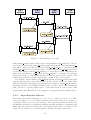
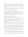
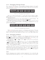
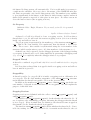
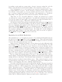
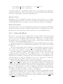
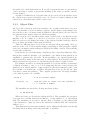
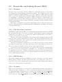
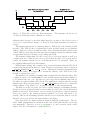
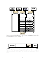
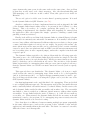
Requests and answers are processed in a diﬀerent way. Figure 2.1 shows the
complete processing cycle of a request-answer pair. The request is pre-processed
19
Figure 2.1: IPC Message Processing
with request preprocess() and post-processed with process request(). The answer is pre-processed with answer preprocess() and post-processed with answer process(). Task A invokes the system call sys ipc call *() to send the request
and sys ipc wait() to receive the answer. Task B invokes sys ipc wait() which
receives the request and sys ipc answer() to send the response. Internally, the
kernel uses the functions ipc call() and ipc answer() to transfer the messages
between the tasks. To sum up, all messages are pre-processed in the context of the
sending task and then post-processed in the context of the receiving task.
For example, when sending a IPC M WRITE request, request preprocess() will
read the data from the source address space (in the context of the source task), while
when the destination task approves the transfer by replying, answer preprocess()
will write the data to the destination address space (in the context of the destination
task). Therefore, only the address space of the current task is ever accessed. This
is important, since HelenOS does not support accessing alternative address spaces.
2.5.4
Asynchronous Library
The kernel delivers IPC messages to a task, not to a thread, let alone to a ﬁbril.
If more threads try to receive IPC messages at the same time, it is a matter of
coincidence which one receives the message. The asynchronous library allows issuing multiple asynchronous requests in multiple threads and ﬁbrils concurrently and
makes sure the replies are delivered to the right recipient (who is waiting for the
reply). It also takes care of creating ﬁbrils to handle incoming connections.
20
In short, the asynchronous library provides a simple and intuitive interface to
the IPC subsystem in context of multi-threaded applications.
2.5.5
Connections and the Naming Service
Tasks in HelenOS can act as servers, oﬀering services to other tasks and also (possibly at the same time) as clients, i.e. consumers of services. Clients talk to servers
over IPC connections.
Connections are managed using the methods IPC M CONNECT ME TO and IPC M CONNECT TO ME. It is not possible for an application to connect to a server directly,
however. Instead, it must use the naming service for this purpose.
The naming service is provided by a task (called the name server). Every task
has a phone connected to the name server. Whenever a task S wishes to oﬀer its
services to other tasks, it registers with the name server using the CONNECT TO ME
message. The name server acknowledges this message, which causes the kernel to
create a new connection in the opposite direction, that is, from the name server to
the task S. The kernel ﬁlls in the phone number of the new connection in the reply
message before returning it to the name server. The name server thus possesses a
connection to every server in the system (and knows their phone numbers).
A client task C wishing to connect to a service sends a CONNECT ME TO message to
the name server and speciﬁes the type of the requested service as an argument. The
name server forwards this message to the respective server. The server acknowledges
the message (replies with zero return value). As a result of this action, the kernel
creates a new connection from task C to task S. Again, task C receives the phone
number of the new connection in the reply to the CONNECT ME TO message.
2.6
Further Reading
It is not possible to describe the various HelenOS subsystems in detail within the
conﬁnes of this introduction. For more details about its design and implementation
you can read the HelenOS Design Documentation ([H-DD]). An explanation how
IPC is used in applications can be found in the excellent tutorial [IPCfD].
2.7
2.7.1
SMC Coherency
Why Self-Modifying Code?
Self-modifying code is code that overwrites itself or, more generally, code that writes
instructions into memory and then executes them. Self-modifying code was used in
the past as a clever hack to write small eﬃcient software in the past. Nowadays it is
’discouraged’ and seemingly rarely used in user applications. This point of view can
be deceiving, however. Any operating system that runs native code is inherently a
clear example of self-modifying code. Any loader writes instructions into memory
to execute them later–again SMC code. Debuggers and dynamic linkers are another
ﬁne examples of SMC. Just-in-time compilers also generate code and run it and
thus eﬀectively contain self-modifying code. Therefore, SMC is not something that
should or could be ‘avoided in all circumstances’. Rather, it is something that does
21
not occur in typical application code itself, but occurs regularly in diﬀerent parts of
the operating system, both in the kernel and in user space.
2.7.2
Contemporary Memory Architecture
Contemporary computer system architectures sport various optimizations to increase speed that are mostly transparent to user applications, but not so to system
software. Of particular problem to us are CPU write buﬀers and various caches.
Let us ﬁrst describe the diﬀerences between the two.
Write buffers are small buﬀers inside each CPU (a few words at maximum).
When a store instruction occurs, the CPU writes the data in the write buﬀer and
continues without waiting for the data to propagate outside the CPU to the system
bus. The CPU is usually aware of data in its own write buﬀers. Thus if another
instruction reads that data later, the data will be (correctly) picked up from the write
buﬀer. A CPU, however, cannot see what is inside another CPU’s write buﬀers. In a
SMP conﬁguration the value cannot be seen by other CPUs until it has propagated
outside the CPU.
Caches are quite the opposite. Caches hold much more data (up to megabytes).
Logically they reside outside the CPU, sitting between the CPU and the system bus.
There may be several levels of caches, but that is not relevant to the point. The
more important fact is that each CPU has its own cache or caches, meaning caches
always come in sets of n on n-processor systems. The data in cache is organized in
cache lines. A cache line is a power-of-two sized, naturally aligned block of memory
(e.g. 32 bytes, 64 bytes, etc.). All cache lines in a cache have the same size.
Caches come in two ﬂavors. With a write-through cache every write goes both
to the cache and to the main memory. With a write-back cache a write only goes to
the cache and the contents of the main memory can thus be stale. A cache always
operates on whole cache lines, never on bytes or words.
Most SMP computer systems implement some level of cache coherency. If a set
A of caches is coherent, then once a value has been written to one caches in A, the
same value will be read from any cache in A. This is ensured by the cache coherency
protocol. Basically the caches snoop on the system bus and will propagate the value
when necessary.
2.7.3
Coherency Problems
One problem with caches is that many systems use two different sets of caches, one
for instructions (I-caches) and one for data (D-caches). The coherency of between
these two sets of caches is sometimes not kept automatically. PowerPC is an example
of such architecture. Coherency between I-caches and D-caches is not kept by the
architecture even between the I-cache and D-cache on the same CPU!
Yet another concern with contemporary CPUs is out-of-order execution of instructions. A memory read barrier ensures no read started before this instruction
ﬁnished. Likewise a memory write barrier ensures all previous instructions writing
have been performed before control proceeds further. Similarly an instruction barrier forces the CPU to discard any data it may have previously fetched into the
instruction pipeline. (This kind of problem is rare, however.)
These are the problems that particularly any loader (or any piece of code that
writes instructions into memory) must be aware of. Between the instructions that
22
write the code into memory and the point where they are executed, a special sequence of instructions must be inserted that makes sure the data (code) are propagated all the way to the instruction pipeline.
2.7.4
Instruction Memory Barriers
A sequence of instructions that propagates data all the way from a write instruction
to the CPUs instruction execution pipeline is called an instruction memory barrier or
IMB by the ARM Architecture Reference Manual ([ARM]). Some of the instructions
are typically privileged, so the operating system must provide a system call for
applications to be able to access this functionality.
The exact instructions that must be executed depend on the speciﬁc system as
some architectures do not specify the cache conﬁguration exactly. However, it is
quite safe to assume the worst possible case for each architecture. The worst that
can happen to us is that we will be doing some extra work.
We will no go through the diﬀerent operations that need to be done during the
course of the IMB. First we may need to issue a memory write barrier instruction
to make sure all store instructions have been performed and the data got as far
as the write buﬀer. Then we must ﬂush the write buﬀers in the CPU that wrote
the instructions to propagate them out of the CPU. After that we must ﬂush the
corresponding entries in the data caches (if the caches are write-back). Hereafter we
must invalidate corresponding entries in instruction caches (if I-D cache coherency
is not maintained). Finally, we might need to issue an instruction barrier instruction
to drain the instruction pipeline and instruction prefetch buﬀers.
This procedure describe above sounds horriﬁc, but fortunately most architectures
ensure a signiﬁcant degree of consistency so only a minority of these steps listed
above is necessary. On the IA-32 architecture, for example, one CPU is always selfconsistent (to ensure backward compatibility with legacy code). On the other hand
the ARM and PowerPC architectures ensure only a small degree of coherency and
consequently require much more eﬀort.
There is a little diﬀerence between the diﬀerent synchronization operations.
Write buﬀers are always in their entirety (i.e. all the buﬀers in one CPU) and
the barrier instructions also have eﬀect on all the data in the CPU. On the other
hand, when ﬂushing or invalidating caches it is usually possible (or even necessary)
to provide an address or range of addresses that needs to be ﬂushed or invalidated.
(Flushing the whole cache would have a severe performance impact on the system.)
2.7.5
SMC Coherency in HelenOS
When the work on this thesis started, HelenOS was completely ignoring the problem
of SMC coherency. The fact that this bug did not manifest itself was partly due to
sheer luck, partly owing to the fact that HelenOS is mainly developed using emulators that mostly do not emulate caches or other architecture features that might
trigger SMC coherency problems. However, the PowerPC port is developed using
the PearPC emulator that actually does emulate caches and I-D cache inconsistency
(within the same CPU) can be observed with this emulator. Here, the fact that
HelenOS was working was probably a combination of sheer luck and the fact that
code was not being executed immediately after being written.
23
Needless to say that with a debugger and a dynamic linker SMC coherency issues
become very visible. A debugger modiﬁes instructions that another task is executing
and a dynamic linker modiﬁes instructions in its own task (at least in some cases).
When the issue was discovered, signiﬁcant eﬀort was put into investigating the
problem and introducing SMC coherency mechanisms into the system. A generic
kernel interface plus a system call have been introduced. These will be described
next. Apart from the kernel ELF loader these are used both by the debugging code
and the dynamic linker.
The problem also concerned the boot loaders. At this point we believe the biggest
holes have been ﬁxed. More work might need to be done for some architectures when
the corresponding HelenOS ports are enhanced to support real systems (that, unlike
architecture emulators, have coherency issues).
The eﬀort resulted in the following two inline functions (or possibly macros) to
the architecture barrier.h headers:
• void smc coherence(void *addr);
• void smc coherence block(void *addr, size t len);
The ﬁrst function operates on a single byte, the other on an entire block. The
functions propagate data all the way from the write instructions to the instruction
pipeline. The policy has been set that after writing any code it should be propagated
through the entire data path as soon as possible using the SMC coherence functions.
We will describe the PowerPC architecture case for illustration. The implementation can be found in kernel/arch/ppc32/include/barrier.h. The PowerPC
architecture requires that each four bytes are ﬂushed separately (unless we can determine from our knowledge of the particular system that the memory system uses
larger cache-line size). The full sequence consists of the following four instructions:
• dcbst addr – Request ﬂushing of memory block into memory.
• sync – Wait until memory has been written.
• icbi addr – Invalidate copy in instruction cache.
• isync – Synchronize and drain CPU prefetch buﬀers.
This sequence is cited by the PowerPC Architecture Manual ([PPC], section
5.1.5.2) as the most common one and it worked for us. On the other hand it
probably does not work on systems with uniﬁed caches (where the icbi instruction
has no eﬀect) so the sequence will need to be modiﬁed to support these systems in
the future.
The block variant smc coherence block() ﬁrst requests ﬂushing of all bytes in
the block by issuing the dcbst instruction for every four bytes of the block. Then
it uses the sync instruction to make sure the dcbst instructions have been actually
carried out. Then it invalidates all potential stale cache lines in the instruction cache
by calling icbi on every fourth byte of the block. Finally it calls isync to make sure
all previous instructions have been completed and to drain the instruction prefetch
buﬀers of the CPU.
The PowerPC architecture case is also interesting since the eﬀects of the coherency issues could be directly observed in the PearPC emulator when using the
debugger that was implemented as part of this thesis.
24
A system call smc coherence was introduced to expose the functionality to
user-space applications. It takes two arguments, the address and length of the
block to synchronize. It simply does some checks and then calls the function
smc coherence block() to do the job.
In the relevant parts of the text we will note when the interfaces described above
were employed to maintain coherency.
25
26
Chapter 3
Debugging and Tracing Overview
3.1
3.1.1
Bugs and Observability
Hunting Bugs
Bugs or defects in functionality tend to appear in every part of software life cycle.
There are many diﬀerent types of bugs and there are many diﬀerent methods of
hunting them. Bugs in large and complex software systems can be extremely diﬃcult
to ﬁnd. To track down such bugs we try to make use of all the diﬀerent options that
are available to us. Anything that can help to pinpoint the bug is a valid option.
Apart from the nature of the bug one can also choose the debugging method
to use depending on the information available to him (source code, symbol table,
type information), the position he ﬁnds himself in (developer, sustaining engineer)
or simply personal preference.
3.1.2
Observability
Observability is a property of a system that allows to infer its internal state by
knowledge of its external outputs. In software engineering observability is extremely
desirable since, in an observable system, one can examine the sequence of events that
has lead to the bug and hopefully ﬁnd its cause.
Observability in a computing system can be attained through its design, debugging output and tools. In real software systems attaining full observability is an
endless battle, as each new tool or programming environment usually requires new
debugging tools to remain observable.
For example, in a traditional operating system, we need a kernel debugger to
observe the kernel and an application debugger to observe the native applications.
However, an application written in an interpreted language cannot be readily observed with the native application debugger and usually necessitates the use of a
specialized tool. A similar situation arises with the proliferation of virtual machines,
such as Microsoft’s CLR (Common Language Runtime) or Sun’s Java Virtual Machine.
3.1.3
Impact
In order to be able to pinpoint any bug that has ever manifested itself, we would
ideally want software to be fully observable. Observability, however, always comes
27
at a price. The design of the system itself is a trade-oﬀ between speed, memory requirements, maintainability, observability and many other factors. Many debugging
techniques can impose extreme overhead to the point where the system is no longer
usable. Therefore, only observability measures with reasonable overhead are used
in production and more sophisticated (and costly) methods are employed once we
start debugging.
Debugging can have other impact on a system than making it run slower or
consume more memory. In a multi-threaded environment, for example, the debugger
can eﬀectively force sequential processing. In such situation, bugs related to multiprocessing may no longer manifest. This makes the debugger unsuitable for solving
this particular problem.
Most debuggers allow altering the state (memory, registers) of a running system.
It is perfectly obvious that such interference can easily put a perfectly correct system
into an incorrect state with possibly fatal consequences. Therefore, such destructive
techniques are almost never used in production systems.
3.1.4
Common Debugging Methods
Basically, we can perform static analysis, live analysis or post-mortem analysis.
Static analysis is used to assess the correctness of software without actually
running it. One obvious example is simply going through the source code and trying
to ﬁnd common programming errors. This can be performed both by humans and
by automated tools. Most importantly, static analysis can be attempted as early as
the design phase of software development.
Live analysis consists of running the software and examining its behavior at
run time. In this case it is possible to experiment and immediately see the results.
With the appropriate tool one can directly modify the code or data of a running
program.
For post-mortem analysis the program is run and some data are recorded
that document what the program was doing when it was executing or just before it
crashed. These can be practically anything, such as debugging messages, memoryusage statistics, a dump of memory contents and so on. The main advantage of
post-mortem analysis is its repeatability.
Next we will look at a few of the most common debugging tools and techniques.
3.1.5
Common Techniques
Debugging Output
From ﬂashing LEDs in embedded devices, through the classical printf to complex graphical output. Debugging messages are simple and eﬀective. The can be
examined at run time or logged and examined post mortem.
Assertions
An assertion is a programming-language construct expressing that a certain Boolean
expression (resembling a logical statement) should be true. The compiler generates
code that veriﬁes this and if the expression evaluates to false, an error is generated. Assertions are usually not compiled into production build and thus only incur
overhead in debug builds.
28
Breakpoints
With a debugger it is possible to designate a set of places in the code as breakpoints.
Whenever control passes through these points in the code, execution is suspended
and the debugger is activated.
Single-stepping
The program is executed one instruction at a time. The user conﬁrms the execution
of each instruction (machine instruction, line of code, etc.)
Watchpoints
Watchpoints are set on areas of memory (a range of addresses, a variable) and the
execution is suspended whenever the memory guarded by the watchpoint is read
from or written to.
3.1.6
Debugging Software
Debugger
A debugger is an application that typically allows to set breakpoints in a running
process, to single-step it and to examine and possibly modify the contents of its
memory and registers. Debuggers come in many diﬀerent varieties depending on
the environment they run in and the environment of the code they are supposed to
debug. The most common kind are simply user-space processes that allow debugging
other user-space processes. Some debuggers, such as the Solaris Modular Debugger
(mdb) can debug the kernel, too. Debuggers also frequently allow performing postmortem analysis on memory dumps.
Kernel Debugger
A kernel debugger is simply a debugger that runs inside the kernel and is usually
most useful for debugging the kernel itself. The advantage of a kernel debugger is
that it is available even if the machine is in such a state that user applications are
no longer working.
Firmware Debugger
Sometimes a debugger is even located in the read-only memory of the computer as
a part of the ﬁrmware. For example, debugging commands can be issued from the
OK prompt of OpenFirmware on SPARC-based machines. This can be useful when
debugging the boot loader or when even the kernel is unable to continue.
Emulator-integrated Debugger
Going even lower, a debugger can be integrated inside the emulator/virtual machine
the software is executing in. Most emulators possess at least some rudimentary
debugging features and some of them have fully-ﬂedged debuggers integrated in
them.
29
Tracer
A tracer allows to record the occurrence of certain events in an application. Most
typically it records the passing of the ﬂow of control in an application through certain points in the code or through an interface. Unlike a debugger tracers do not
suspend the execution of the application. This makes it possible to use a tracer without disrupting the normal operation of the software, if the tracing is implemented
eﬃciently.
The UNIX tool strace, for example, traces system calls made by a UNIX process
and the signals delivered to it by the system. The DTrace tool allows tracing many
diﬀerent types of events in the kernel and in applications.
3.1.7
Data for Post-Mortem Analysis
A log is a recording of the occurrence of certain events in an application. It can
be produced as simply as redirecting the debugging messages in a ﬁle or it can be
machine readable and used to produce sophisticated statistics or analysis.
Memory Dumps can also be machine readable and they can usually be examined with a debugger, just as a live process. The ELF ﬁle format can store memory
dumps in addition to its more well-known uses.
3.1.8
Methods for Static Analysis
Code Review is a process where the same code is read and analyzed by several
people. This is an example of static analysis performed by humans.
Lint was a tool for static analysis of C code that allowed to ﬁnd non-portable
constructs and constructs that were likely to be bugs. Contemporary compilers oﬀer
the same functionality through enabling warning messages.
Locking Analysis is a restricted variant of formal veriﬁcation. For example,
the Linux kernel uses automated tools to verify locking schemes and look for possible
deadlocks.
Formal Veriﬁcation: A formal speciﬁcation of the desired behavior of the
system can be developed and a formal proof of correctness constructed. Tools called
proof assistants have been developed especially for the purpose of checking such
proofs.
It should be noted, however, that even a formally veriﬁed program can only
be bug-free to the point the formal speciﬁcation is bug free. In other words we
might not succeed in encoding our real intent properly in the formal system used
for the proof. This method is more suited to small, mission-critical and well-deﬁned
systems (such as ﬂight control systems) or speciﬁc subsystems, but less suited to
large, complex and vaguely speciﬁed systems, such as application suites.
Another approach, more suitable to complex systems, is to logically divide the
system into components and to specify the way they are allowed to interact. Such
approach is commonly used in software componentry and design by contract.
3.2
Breakpoint Debugging Support in Processors
Some processor architectures have direct hardware support for breakpoints and
watchpoints. However, this hardware support is extremely limiting in the num30
ber of breakpoints or watchpoints that can be set. On IA-32 it is only possible to
set four, for example. Many processor architectures lack any hardware support at
all.
Fortunately, most architectures possess some kind of a break instruction (or a
suitable substitute). The debugger instruments the code of the application by overwriting the instruction at the breakpoint address with the break instruction. Also,
single stepping can be implemented using breakpoints. This will be explained in
greater detail in the implementation section.
Watchpoints can be implemented using the MMU. The page containing the variable being watched is either removed from the page tables or the access to it is
restricted. When an access to the page is made, the page fault handler evaluates
whether the watchpoint has been hit or not. This method can have large overhead,
though, as the page is often contains other variables and any access to these triggers
a page fault.
3.3
Network Packet Analysis
One area where this thesis draws its inspiration from are network packet analyzers,
such as Wireshark. The traﬃc is usually intercepted at link level (i.e. very low level).
The analyzer partially mimics the functionality of the network stack to reconstruct
data from higher levels. There is practically no limit to this concept, transport
streams and even application protocols can be reconstructed.
31
32
Chapter 4
Debugging and Tracing Design
and Implementation
4.1
Design Overview
Our aim was to design and implement an operating-system facility that would allow
debugging and tracing of tasks by other tasks. We would also develop two example
applications, a system call tracer and a simple debugger.
During the design process, we had several goals on our mind. The code should
be modular and portable, there should be a minimum of platform-dependent code.
The kernel should contain only the functionality that absolutely must reside in the
kernel. The kernel part should provide mechanism, but not policy.
It is also important to stress that a debugging mechanism of an operating system
is second in importance to the regular operation of the system. It follows that it
is better for the debugging facility to be somewhat slower and more complicated,
rather than make the regular operation of the kernel slower or complicated (e.g. by
sacriﬁcing some optimizations).
The kernel facility was named udebug, meaning support for user-space debuggers.
Note: In the text concerning the kernel debugging facility, the term application
refers to the task being debugged. The term debugger refers to the task connected to
the application via the debugging facility. It can thus refer both to the breakpoint
debugger application and the system-call tracer application.
We will now outline the main components of the design. The kernel exposes
a set of debugging methods through the IPC interface and the HelenOS C library
provides a convenient wrapper to this interface. The methods allow one task (the
debugger) to enter a debugging session with another task (the application). Then
the debugger can read and write the contents of the registers and memory address
space of the application and it can opt to be notiﬁed of several diﬀerent events in
the application’s threads (such as the application performing a system call, hitting
a break instruction, etc.)
The debugger is fully responsible for managing the threads of the application,
setting breakpoints by modifying the code, understanding the contents of CPU
registers and so on.
33
4.2
Supported Architectures
Only a certain subset of the kernel facility is necessary for implementing system-call
tracing. This subset is interesting, because it is completely portable. It contains no
architecture-dependent code, let alone assembler code.
Therefore, once some 64-bit issues have been addressed, the tracing functionality
started working on all architectures supported by HelenOS. For this reason, the
tracing part has already been integrated into the trunk.
The debugging part requires a small amount of architecture-dependent code in
the kernel (speciﬁcally, the code to translate hardware debug exceptions to udebug
events. The bulk of the architecture-dependent code is in the Breakpoint Debugger application. In short, the arm32, ia32, mips32 and ppc32 are supported for
debugging to various degrees.
4.3
4.3.1
Udebug Interface
Interface Form
Anytime one implements some functionality in the kernel that should be exposed
to user space, he is faced with the choice of which existing kernel-to-user-space
transport mechanism to extend to accommodate this functionality. (Supposing we
do not want to introduce a completely new one.) On a UNIX-like system, there
are several possibilities: system calls, ioctls, pseudo ﬁle systems, etc. On HelenOS
pseudo ﬁle systems are out of the question as the kernel knows nothing about ﬁle
systems.
The ﬁrst idea was to introduce a set of new system calls and we created a
prototype implementation of this interface. Nevertheless, in the end we agreed that
basing the interface on IPC would not only be more elegant, but also much more
convenient for the application, as it can take advantage of the asynchronous library.
4.3.2
Connecting
The ﬁrst thing a debugger needs to do is to create an IPC connection to the application. Unlike with connecting to a service, there is a system call provided to
connect directly to a task speciﬁed by its ID. (The task ID is an unsigned 64-bit
integer that uniquely identiﬁes the task within a running system.) The system call
is ipc connect kbox and takes a single argument, the task ID.
Now this system call does not create a connection to the regular answerbox associated with the application task. That would cause messages to be connected to
the application and it would have to participate in the communication. That is deﬁnitely not what we want as the debugging process should be completely transparent
to the application.
Instead, this system call creates a connection to an alternative, hidden answerbox, the kernel answerbox alias kbox. The kbox is an answerbox associated with
each task. The answerbox is not accessible to the user-space code of the task, it is
managed by the kernel.
34
4.3.3
Debugging Message Format
Once connected, the debugger can start sending debugging messages to the application. The table 4.1 shows the general IPC message format and how its ﬁelds are
used in debugging messages.
Method
IPC M DEBUG
ARG1 ARG2 ARG3 ARG4 ARG5
dm
da1
da2
da3
–
Table 4.1: Debugging Request Structure
The top row lists the ﬁeld names of a generic IPC message (Method, ARG1–
ARG5) while the bottom row shows how these ﬁelds are used to hold the ﬁelds of
the debugging message.
The ﬁrst ﬁeld from the left is the method number in request messages. All
debugging messages use the same system method IPC M DEBUG.
The diﬀerent debugging methods are distinguished by their debugging method
number (dm) which is passed in ARG1. The debugging arguments (da1 –da3 ) are
passed in ARG2–ARG4.
Retval
0 or Exxx
ARG1 ARG2
dv1
dv2
ARG3
dv3
ARG4
–
ARG5
–
Table 4.2: Debugging Reply Structure
Table 4.2 shows the generic structure of a debugging reply messaeg. The reply
to every debug request has the return value 0 on success or negative error code on
failure. Some methods return additional values in some of the ARG1–ARG3 ﬁelds.
4.3.4
Debugging Methods
All the names of symbolic constants for the debugging methods have the form
UDEBUG M method where method stands for the capitalized name of the method. The
debugging methods that have been deﬁned are listed in table 4.3.
From these the regs read, regs write and mem write methods are not used by the
tracing application.
We will use the notation the method(a, b) → (–, c, d) to denote a method named
‘the method’ that has two arguments a and b (where a is passed in ARG2 and b
is passed in ARG3). It also returns two additional values (apart from the return
value), c and d in ARG2 and ARG3.
Most of the methods do not block, meaning they should return reply without
substantial delay, unless explicitly stated otherwise. The kernel veriﬁes whether the
methods have been used in an appropriate context (i.e. the args read method can
only be used with a thread that is suspended in a syscall event. If the request is
used in an inappropriate context, it returns an error.
begin
Opens a debugging session with the recipient (application). As a side eﬀect this
suspends all threads in the application. As soon as all the threads are safely stopped,
35
Method Name
begin
end
set evmask
guard
go
stop
args read
regs read
regs write
thread read
mem read
mem write
Description
Begin a debugging session.
Terminate the current debugging session.
Enable and disable different events.
Notify when debugging session terminates.
Resume a thread until an event occurs.
Suspend a thread.
Read system call arguments.
Read user-space register context.
Write user-space register context.
Read list of threads in the task.
Read application memory.
Write application memory.
Table 4.3: Debugging Methods
it returns zero.
If somebody is already debugging this application, the request returns the error
code EBUSY.
end
Closes the debugging session. This has the eﬀect of answering all pending requests.
set evmask(mask)
Selects which events should be watched for in the application. The argument mask is
a bit mask that can be constructed using the constants UDEBUG EM XYZ. Here XYZ
is one of FINISHED, STOP, SYSCALL B, SYSCALL E, THREAD B, THREAD E, BREAKPOINT,
TRAP. (B stands for begin, E for end). The individual event types will be discussed
in detail later.
guard
This method does not return a reply until the debugging session has ﬁnished. It
does not have any other side eﬀects. It can be used to detect that the application
has been killed even if the application us suspended at that time. This method has
not been implemented yet.
go(hthread) → (evtype, v1 , v2 )
Resumes the thread identiﬁed by the hash hthread, allowing it to run until a debugging event occurs. This method does not return a reply until an event has occurred
in the thread (and as such it can block indeﬁnitely). When a debugging event does
occur, the thread is suspended and a reply is sent. – Resume a thread until an event
occurs.
36
stop(hthread)
Requests a stop event to be generated in the thread hthread. This has the eﬀect of
suspending the thread and returning a reply to the current pending go request.
args read(hthread, buf ptr)
Reads system call arguments. When the thread hthread is suspended in a systemcall event (SYSCALL B or SYSCALL E), this method will copy the arguments of the
system call to the buﬀer pointed to by bufptr. The buﬀer should have enough space
to hold the maximum number of system-call arguments, which is six in the current
implementation of HelenOS.
regs read(hthread, buf ptr)
Reads user-space register context of the thread hthread into the buﬀer pointed to by
bufptr. It can only be used for threads suspended inside a breakpoint or a trap event.
Here bufptr should point to an istate t structure, which is architecture-speciﬁc and
it is deﬁned in the kernel headers.
regs write(hthreads, buf ptr)
Sets the user-space register context of thread hthread to the values read from bufptr.
As with regs read, the bufptr argument should point to an istate t structure.
thread read(buf ptr, buf size) → (–, bcopied, bdatasize)
Reads the list of threads in the application to the buﬀer pointed at by bufptr, writing
at most bufsize bytes. The data is written as a vector of hashes. The reply contains
additional values, bcopied and bdatasize. Here bcopied is the number of bytes that
were actually copied and bdatasize is the total number of bytes that were available
(which is the size of a pointer times the number of threads in the application). This
can be used to detect that the buﬀer provided was too small to hold the entire list.
mem read(vaddr, buf ptr, buf size)
Reads bufsize bytes from the virtual address vaddr in the application’s address space
to the buﬀer pointed to by bufptr. If there is no mapping for the speciﬁed address
range, the request will fail.
mem write(vaddr, buf ptr, buf size)
Writes bufsize bytes from the buﬀer pointed to by bufptr to the virtual address vaddr
in the application’s address space. If there is no mapping for the speciﬁed address
range, the request will fail.
4.3.5
Typical Debugging Session
After connecting to the kbox of the application, the debugger issues a begin request.
This suspends all the threads in the application and a reply is returned. The debugger then uses the thread read request to obtain a list of threads in the application
(their hashes, actually).
37
The debugger issues a begin request concurrently for each thread. The threads
resume execution. When an event occurs in a thread, the thread is suspended and
a reply is returned for the appropriate request. The debugger uses other requests
to determine details about the event and then issues a new begin request to resume
the thread again.
4.3.6
Events
Udebug deﬁnes several diﬀerent events. The type of an event is an integer corresponding to one of the UDEBUG EVENT evname constants. (E.g. UDEBUG EVENT STOP
for the stop event.)
Information about an event that has occurred in a thread is passed to the debugger in the reply to the go request for that thread. The format of the message is
shown in table 4.4.
Retval
0
ARG1 ARG2
evtype
v1
ARG3
v2
ARG4
–
ARG5
–
Table 4.4: Debugging Event Message Structure
The return value should be zero (for success). ARG1 contains the event type
evtype. ARG2 and ARG3 can hold additional values v1 , v2 associated with the event.
Their meaning depends on the type of the event. Keep in mind that the identity of
the thread which triggered the event is also there, even though it is implicit.
We will now discuss the individual event types and their meaning. We will denote
evname(a, b) an event with associated values a and b.
Finished Event
When the debugging session ends for whatever reason, all outstanding go requests
return the finished event.
Stop Event
The debugger can request this event to be generated by issuing a stop request. It is
used to stop a thread explicitly.
Syscall B(id) Event
The syscall B event is generated upon the entry to a system call handler. The id
value tells us the system call number, i.e. it identiﬁes the system call that has been
invoked.
Syscall E(id, rc) Event
The syscall E event is generated upon leaving a system call handler. Again, id is
the system call number. The other value, rc, is the result code of the system call,
i.e. the value returned by the system call.
Since some system calls can take indeﬁnitely long to return, it is very useful to
have an event for both entering and leaving the system call handler.
38
Thread B(thash) Event
When a thread t1 in the application tries to create a new thread t2 (with the
thread create system call), the newly created thread starts suspended (it does
not execute any user-space code). The thread B event is delivered to the thread t1 .
The thash value is the hash of thread t2 .
Thread E Event
When a thread ﬁnishes executing for whatever reason, it generates the thread E
event.
Breakpoint(value) Event
The breakpoint event is generated when the thread hits an architecture-speciﬁc break
instruction. This is INT3 on ia32, bkpt on arm32, BREAK on mips32 and trap on
ppc32. The break instruction generates an architecture-dependent exception that
gets translated into the breakpoint event.
The value is architecture-dependent. The idea is that some architectures allow
incorporating a numeric value into the opcode of the break instruction. Currently
it is not used.
Trap Event
On architectures that have hardware support for single-step tracing, this event is
generated after executing each instruction. The single-step tracing must be ﬁrst
enabled in an architecture-dependent way.
The only architecture currently supporting this is ia32. The single-step tracing
is enabled by writing one into the trap ﬂag (TF) of the EFLAGS register (which
can be done with the method regs write).
4.4
4.4.1
Udebug Implementation
Implementation Overview
Udebug keeps per-task and per-thread state in structures of type udebug task t and
udebug thread t, respectively, embedded directly in each task and thread structure.
The implementation itself is designed in a modular fashion. The bulk of the code
resides in four modules, three of them can be found in the directory kernel/generic/src/udebug (udebug.c, udebug ipc.c, udebug ops.c) and the last one is
kbox.c in kernel/generic/src/ipc and some new functions were added to kernel/generic/src/mm/as.c.
The code that runs within the context of the application resides in udebug.c.
Apart from code to initialize and clean up the data structures, this module most
importantly contains the various hooks that are inserted to the appropriate places
in the kernel to trigger debugging events.
The udebug ops.c module provides a set of functions that are used to implement
the various debugging methods. (For example, a the function udebug set evmask()
sets the event mask.) Most of these functions are executed in the context of the
debugger task.
39
The kbox.c module manages the kernel answerbox for that task, that we already
mentioned in 4.3.2. This is where the phone is connected for debugging the task.
The main job of this module is to create a kernel-only service thread in the task,
the kbox thread, whenever a phone is connected to it via ipc connect kbox().
The last module, udebug ipc.c provides binding of the debugging operations
module to IPC and also implements the main function of the kbox thread. This
function acts as a server that participates in performing certain debugging operations.
The corresponding header ﬁles are kbox.h in kernel/generic/include/ipc and
udebug.h, udebug ipc.h, and udebug ops.h in kernel/generic/include/udebug.
Of these, the most interesting is the ﬁle udebug.h, which deﬁnes the enumerations
for the debugging method number, types of debugging events and the per-task and
per-thread data structures udebug task t and udebug thread t.
The entire udebug facility can be enabled or disabled using the conﬁguration
option Support for userspace debuggers (CONFIG DEBUG). When disabled, udebug is
not compiled into the kernel. The ipc connect kbox() system call is then replaced
with a stub that returns an error code (ENOTSUP).
4.4.2
Suspending and Resuming Threads
The Challenge
The begin and stop requests allow suspending an application thread (threads). This
is not a simple operation, due to several factors. On a multiprocessor machine the
thread can be executing on a diﬀerent CPU at the time we are trying to suspend it.
On the other hand, the thread can be blocked in a system call and not executing at
all.
Begin is used to start debugging an application and stop is usually used to pause
its execution (when the user hits a pause key in the debugger). Therefore, it is not
necessary for the request to be completed really quickly. What we do require is that
the request be satisﬁed in reasonably short time regardless of what the application
is doing.
If the application is busy executing, it is either calling into the system, or, if it is
not making system calls, it is being preempted repeatedly. In this case it would be
suﬃcient to put stopping points to the system-call handler and preemption handler.
In these stopping points the thread would check whether it is supposed to stop. If
so, it would block and inform the debugger (by sending a reply to the go request
containing the stop event).
Things are never so simple, however. A thread can be blocked in a system call
indeﬁnitely, in which case it could not reach a stopping point within the reasonably
short time interval. Two possible solutions to this problem have been considered.
The ﬁrst solution is to identify sleeping threads as such and mark them as suspended. The thread would not get scheduled until it was resumed. This would
require extending the scheduler to understand this concept.
Another solution is to deﬁne stopping sections. If the thread is requested to
stop, it is guaranteed not to pass through or leave a stopping section. Having such
construct at our disposal, it suﬃces to place a stopping section at the right place in
each blocking system call.
The ﬁrst solution mentioned is more universal in that it would cover any poten40
tial future blocking system call automatically. Yet it would make it necessary to
complicate the scheduler. Moreover, due to the nature of the SPARTAN microkernel, there are presently only four blocking system calls. The number is very unlikely
to grow signiﬁcantly in the future, as the kernel is fairly feature-complete and most
future development is expected to take place in user space. For these reasons we
chose the latter solution (the stopping sections).
Go Property
102:28:08 Duke: Eagle, Houston. If you read, you’re Go for powered
descent.
Apollo 11 Lunar Surface Journal
A thread is Go iﬀ it is allowed to leave a stopping section. It follows that a
thread that is not Go will reach the nearest stopping section (if it is not already
inside one) and will not leave it.
The Go property is represented by the member go of the structure udebug thread t. This is a Boolean variable. If it equals true then the thread is Go and vice
versa. The access to this variable is synchronized using the lock member of the
structure (which synchronizes access to all other members of the structure, too).
A thread can only be given Go by the debugger by means of the debugger issuing
a go request. A thread can loose Go either implicitly by generating a debugging event
(e.g. syscall B) or explicitly when the debugger issues a stop request.
Stopped Thread
A thread is considered stopped if and only if it is not Go and it is inside a stopping
section.
It follows that a thread that is stopped is inside a stopping section and will not
leave it until it is given Go.
Stoppability
A thread is said to be stoppable iﬀ it is inside a stopping section. Otherwise it is
not stoppable. The Boolean member stoppable of the udebug thread t structure
tracks whether the thread is stoppable or not at the given moment.
In addition, the member not stoppable count of udebug task t tracks the current number of threads in the task that are not stoppable. We will explain the
purpose of this ﬁeld later.
Stopping Sections
Stopping sections are delimited with the calls to udebug stoppable begin() and
udebug stoppable end().
The function udebug stoppable begin() checks whether the thread is Go. If
not, it replies to the outstanding go request, informing the debugger that the thread
is now stopped. (Keep in mind that, by deﬁnition, the thread became stopped at
this instant.) It also marks the thread as stoppable.
The function udebug stoppable end() checks whether the thread is Go. If not,
it blocks, waiting for Go. If the thread is Go, it transitions the thread to the not
41
stoppable state and allows the execution to continue. Of course, the check and the
state transition must be performed atomically.
Performing a Stop Request
With the above deﬁnitions, it is easy to explain how the stop request is implemented.
(The debugging lock of the thread is held to ensure the operation is atomic.)
Go is taken away from the thread by setting the go member to false. If the
thread is stoppable at the moment, it has been eﬀectively stopped so a reply to the
outstanding go request is sent.
If the thread is not stoppable, on the other hand, no further action is performed.
The reply to the outstanding go request will be sent by udebug stoppable begin()
when the thread enters a stopping section.
In any case, the reply to the stop request is sent immediately. The behavior of
the stop request is thus asynchronous in the sense that merely getting a reply to
the stop request does not mean the thread is stopped. Rather, the thread can be
considered stopped when the stop event is received by the debugger (as the reply to
the outstanding go request).
Implementation of the Begin Request
The begin request is a little more complicated. Since all threads must be stopped
until the debugger issues relevant go requests, the kernel must stop all threads in
the application as part of processing the begin request.
This is where the not stoppable count variable is used. If it reads zero at the
time of processing the request, then we are done. The threads are not Go and they
are stoppable so they are already stopped. We can send a reply to the request
immediately.
In the other case we do not send a reply. Inside udebug stoppable begin() the
not stoppable count is decremented. At the same time we check whether the result
is zero. If yes, then this thread has been the last thread that was not stoppable.
Now all threads are stoppable and so they are stopped. Thus, we send the reply to
the begin request.
Example Start-Up and Termination of a Session
The ﬁgure 4.1 shows a debugger starting and terminating a debugging session with
an application. The debugger ﬁrst issues a begin request. The control passes into
the kernel. The kernel starts setting the active ﬁelds of the application threads
to true. In this example, the debugger started with t2 , then it proceeded with t1 .
(Here t1 .d and t2 .d are shorthands for t1 .udebug and t2 .udebug, respectively.)
However, t2 is not in a stopping section so it takes a while for it to stop. Meanwhile the kernel sets t1 .d.active to true and since t1 is in a stopping section, it
is stopped immediately and the nsc (not stoppable count) of the application is
decremented. Some moments later t2 enters a stopping section and decrements nsc.
Since t2 was the last thread outside a stopping section, the value of nsc is now zero.
Therefore, t2 sends a response to the original begin request.
The termination of the debugging session is much simpler. The debugger issues
an end request. The control passes into the kernel. The kernel sets the active ﬁeld
42
Figure 4.1: Debugging-Session Management Example – A debugging session is initiated with an application (running two threads) and then terminated.
in the debugging structure of t1 and t2 to false. Then, without waiting, it sends a
response to the end request and returns control to the debugger.
4.4.3
Hooks
Hooks (calls to udebug) are inserted at strategic spots in the kernel. These fall into
one of the following categories:
• State management – State structure initialization and cleanup.
• Event hooks – Generate debugging events and suspend the threads.
• Stopping section delimiters – udebug stoppable begin/end()
The distinguishing characteristic of the hooks is that they are executed directly
in the context of the application threads (in kernel space, of course). Other Udebug
routines are executed either in the context of the debugger or in the context of the
kbox thread.
State-Management Hooks
The functions that initialize the debugging structures are simply called during the
initialization of the corresponding thread or task structure in which they reside. No
special cleanup is required before de-allocation, as at that time there can no longer
be any active debugging session and there are no dynamic data that would need
freeing.
43
Event Hooks
For the syscall B and syscall E events, the hooks are located in the function syscall handler() in kernel/generic/src/syscall/syscall.c. For both events,
the hook function is udebug syscall event().
The hooks for the thread B and thread E events reside in the functions sys thread create() and thread exit(), respectively, inside the module kernel/generic/src/proc/thread.c. The hook functions are udebug thread b event attach() and udebug thread e event().
The breakpoint and trap the event hooks are inserted into the architecturespeciﬁc exception handlers. The hook functions are udebug breakpoint event()
and udebug trap event().
The remaining events are not generated by event hooks. The finished event is generated during kbox cleanup. The stop event is sent either from udebug stoppable begin() or directly from the function udebug stop() that handles stop requests.
Stopping Section Delimiters
The stopping section delimiters are udebug stoppable begin() and udebug stoppable end(). An empty stopping section (i.e. enclosing no additional code) will be
called a stopping point.
Basically there is a stopping point in the generic system-call handler syscall handler() and in the clock interrupt handler. These two allow stopping both
threads that invoke non-blocking system calls and threads that do not call into
the system at all.
Finally, there is a stopping section in each of the four blocking system calls.
These are arranged so that there is no code with some visible side eﬀects in the
stopping section, just the code that waits for some event to happen.
4.4.4
Task Memory Access
Reading and Writing Memory
The read and write debugging methods allow the debugger to access the memory
address space of the application. Needless to say, there are some obstacles that need
to be overcome.
Address Spaces
As we already explained in 2.5.3, only the one address space can be accessed in
HelenOS at the same time and this is normally the address space of the current
task. HelenOS does not have provisions for accessing an alternate address space. (It
is however possible that such facility might be implemented in the future.)
In any case, we decided to make use of the unique characteristics of HelenOS
IPC to do the job. This is also the place where the kbox thread comes into play.
In an ordinary IPC write operation, the data is ﬁrst copied by the kernel from
the source address space to a kernel buﬀer as part of pre-processing the request. The
address of this buﬀer (which gets allocated from the kernel heap,) is stored in the
buffer ﬁeld of the message structure call t.
The message is delivered, i.e. the kernel switches to the destination task (and
thus to the destination address space), and the user-space code accepts the data
44
by sending a reply with zero return value. As part of pre-processing the reply, the
kernel copies the data from the kernel buﬀer to the destination address space.
Now a debugging read or write request is processed in a similar fashion. There
is a slight diﬀerence, however. As the message is delivered to the kernel answerbox, instead of the regular one, it is processed by the kbox thread. Moreover, no
pre- or post-processing is performed on the side of the application (i.e. the kbox).
Everything on the application side is thus in the hands of the kbox thread.
Thus there are two observable diﬀerences. Firstly, the transaction is carried
out without the consent of the application. Secondly, kbox bypasses the memory
access mode restrictions that apply to the application by using an alternate way of
accessing the memory space. This will be detailed further on.
One purely technical trick perhaps worth mentioning is that process answer()
does not switch on the method number. We did not need to change this behavior,
since we reused the same answer format that was used for IPC M READ for implementing UDEBUG M READ (the read debugging method). In both cases the
data from the buﬀer passed in the answer is to be written to the address space of
the requester (debugger) by standard means. We simply ﬁll out the destination
address and buﬀer length to the same ﬁelds where they are stored for replies to
IPC M READ and process answer() does the rest.
Bypassing Access-Mode Restrictions
The standard way to access application memory from within the HelenOS kernel are
the functions copy from uspace() and copy to uspace(). These will return failure
if either some of the range of accessed addresses is not mapped or if the access mode
does not allow that particular type of access.
Memory areas containing executable code are always read-only in HelenOS. Still,
the debugger needs to modify the code to in order to insert breakpoints. For this
reason copy to uspace() cannot be used. Therefore we use an alternate way to
write application memory. Conversely, we might want to read from a memory area
that does not allow reading to the application. This case is a little bit artiﬁcial, as at
the time of writing there is no such case in HelenOS. For this reason, we decided to
ignore this case for the time being and use standard copy from uspace(). Adding
support for this is similar to the write support (and is actually somewhat easier).
Let us consider the writing support once more. The ﬁrst thing that comes to
mind is simply obtaining the physical frame number from the memory manager and
writing directly to that frame. The HelenOS kernel maintains a 1:1 mapping of the
physical memory in kernel virtual address space. Thus, physical memory can be
accessed directly. All we have to do is to translate the memory by adding the base
address of the mapping. The macro PA2KA() implements this.
Now this would land us in serious trouble pretty quickly. The page in question
need not be present in physical memory. Even if it is (and thus the physical frame
number is valid), it could by mapped into other tasks at the same time or in the
future. The memory area could be shared between diﬀerent tasks and we would be
thus modifying the memory of multiple tasks at once (which surely is not what we
wanted to do). In the latter case, the page could belong to the ELF backend, for
example. When another task is created from the same executable image in memory
(as frequently happens with the program loader, see 6.4). Then the code of the new
task would be cluttered with the changes we made in the original task, too.
45
Therefore, we adopt the following strategy. First we make sure the memory area
we are about to write is private (i.e. not shared) and anonymous (backed by the
anonymous memory backend). When writing, we proceed page by page, making
sure every page is present in memory before writing it.
This requires some new functionality in the memory management subsystem,
namely the module as.c in kernel/generic/src/mm. We implemented the functions as area make writeable() and as debug write().
The function as area make writeable() checks whether the given memory area
is private and anonymous. If it is not, the function makes a copy of the data in the
memory area and replaces the old memory area with a freshly created one, private
and anonymous and containing the same data.
The function as debug write() splits the address range to be written to on page
boundaries and for each piece it uses a helper function debug write inside page().
This function checks whether the page to be written to is present in memory. If it
is not, it calls the page-fault handler to fetch the page. Then it performs the write
itself.
The implementation of the function will remain valid even when paging out is
implemented in HelenOS (as now it is not). The function makes sure the page stays
present by holding locks on the address space and memory area.
4.4.5
Kbox Thread Benefits
We have already seen that the kbox thread plays an important role in accessing the
memory of the application. But that is not its sole purpose.
Actually all debugging requests are mostly processed in the context of the kbox
thread. The only exception is that accessing the memory of the debugger is performed in the context of the debugger (naturally). The beneﬁt here is that it greatly
simpliﬁes locking.
There are actually two ways in which this makes our life easier. One is locking
order and the other is ensuring continued existence.
Firstly, if we tried to work with the current task (the debugger) and with the
application (or their threads), we would need to be extremely careful not to run into
a deadlock. Secondly, the current task and the current thread are always guaranteed
to exist, while the continued existence of other tasks and threads must be ensured
by some means. One could hold a lock on them, for example, but this creates yet
more locking-order issues.
During development we actually created an implementation that performed most
of the processing in the context of the debugger (i.e. during pre-processing). It was
doable, however, by moving the processing to the kbox thread, the locking scheme
was simpliﬁed by an order of magnitude.
4.4.6
Register State Access
User-Space Register State
There are two points where the control can pass from user space to the kernel (and
back). The ﬁrst one is a system call (i.e. the function syscall handler() and the
second one is an exception (i.e. the function exc dispatch().
46
When the kernel is entered by issuing a system call, the user-space register
context is not well deﬁned apart from the program counter, as the general-purpose
registers will be generally clobbered by the kernel.
Upon entering the kernel through the raising of an exception, the architecturespeciﬁc assembly handler saves the user-space register context at the bottom of
the kernel stack of the current thread. The data is saved in accordance with the
deﬁnition of the C structure istate t (which is architecture-speciﬁc). In addition, the assembly routine passes a pointer to this istate t as an argument to the
generic (C language) exception handler exc dispatch(). In the present implementation we store a copy of this pointer to the per-thread debugging state structure
udebug thread t and use it to access the register state.
Allowing access to the program counter when the thread is inside a system call
is a planned feature. It is slightly complicated by the fact that we do not want to
pass any extra argument to the syscall handler() function (it could no longer be
passed via registers as there are too many arguments already). The program counter
thus must be picked directly from the stack (i.e. we need to determine the address
where it is stored).
Missing Register Issues
Unfortunately, HelenOS does not always save the contents of all registers in the
istate t structure. Many architectures have the conﬁguration option ‘Save all
interrupt registers’. Answering no to this question results in a special optimization
to be used.
As the function exc dispatch() conforms to the ABI, it must not clobber the
contents of preserved registers (as deﬁned for the respective architecture). Thus,
there is no need for the assembly routine to save these registers in the istate t
structure.
For Udebug, however, this is very inconvenient. Granted, the values of the registers are stored somewhere, but ﬁnding out where they are is practically impossible.
On SPARC only three registers (pc, npc and state) are saved into the structure and
all the remaining registers are preserved with the help of the register stack engine.
A solution to this problem has been proposed, but it has not been implemented
yet. In fact the solution is to introduce another feature into Udebug that will allow
the user-space debugger to retrieve the register contents itself (with a little help
from the kernel).
The required (or strongly advisable, at least) kernel feature is the ability to map
some anonymous memory into the virtual address space of the application. (This is
actually quite simple). With this feature in place, thunks can be implemented.
Here, thunks are pieces of code injected by the debugger into the address space of
the application (in some unused portion of the address space). The debugger then
forces the application to execute the code by modifying its program counter (which
is always accessible through istate t).
The debugger can then employ thunks to save the register contents to some
pre-arranged area of memory in the address space of the application.
47
Security Considerations
While most registers stored in istate t are user-accessible, there might be from
time to time some registers (or bits of some registers) that the debugger should not
be allowed to modify.
This should be taken into consideration and the relevant registers or bits should
be left in their previous state when performing a regs write operation. Our implementation does not address this issue yet.
4.4.7
Synchronization and State Management
Task State
Per-task debugging state is kept in a structure of type udebug task t embedded
directly in the task structure. This structure contains several ﬁelds. The debugging
lock for the task (a mutex), a pointer to an outstanding begin request (so that we
can reply to it when ready), the number of threads in the task that are not stoppable
(not stoppable count), a pointer to the task structure of the attached debugger
(or NULL if none) and the current event mask. The event mask determines which
events are to be generated and which are not. (Not all events can be disabled in the
current implementation).
Last, but not least, the dt state member determines one of three debuggingsession states of the task, Inactive, Beginning or Active. (See ﬁg. 4.2) When in
the Inactive state, the task is not being debugged (i.e. there is no active debugging
session). When a debugger issues a begin request, the application task transitions
into the Beginning state. This state causes all the threads in the application to stop.
When all threads are stopped, the task transitions into the Active state. The Active
state means there is a debugging session in progress.
When the debugger issues a end request (or disconnects), the application transitions back into the Inactive state. This causes all the threads in the application
to resume execution.
Thread State
Per-thread debugging state is held in a structure of type udebug thread t. Again,
this structure contains a considerable number of ﬁelds. There is a debugging lock
for the thread (a mutex), a wait queue on which the thread waits for Go, a pointer
to the currently pending go request, a buﬀer for system-call arguments, a pointer to
the user-space register state and the type of the current debugging event.
Perhaps the most interesting ﬁelds are the Boolean go ﬁeld, that reﬂects whether
the thread is Go, the stoppable ﬁeld, that determines whether the thread is stoppable at the moment and ﬁnally the active ﬁeld.
The active can be regarded as a copy of the dt state ﬁeld from the task state.
It allows determining whether there is an active debugging session when operating
on a thread, without the need to examine (and lock) the task itself.
Kbox State
The beneﬁts of the kbox thread come for a price as there is some eﬀort connected
to managing it. The thread must be created automatically when someone connects
48
Figure 4.2: Debugging State Transitions
to the kbox. It should terminate when all phones are disconnected from the kbox
and it deﬁnitely must be destroyed before the task is dismantled.
The state needed to manage the kbox is held in a structure of type kbox t
(deﬁned in kernel/generic/include/ipc/kbox.h) which is directly embedded in
the task state (the kb ﬁeld). The structure contains the answerbox itself and a
pointer to the kbox thread structure. There is also a mutex called cleanup lock
and a Boolean variable finished that serve to synchronize cleanup of the kbox
thread.
Locking Scheme
The kbox t and udebug task t structures reside in the task t structure of the task
they belong to. The udebug thread t structure resides in the thread t structure
of its thread.
The access to kbox t is synchronized simply with the same spinlock that synchronizes the access to the whole task t structure in which it resides.
On the other hand, each udebug task t and udebug thread t structure contain
a mutex with the name lock that synchronize access to these structures.
To access a task or thread debugging structure, you must hold the lock mutex
in it and ensure its continued existence. On the other hand, holding the spinlock of
the task or thread is not required.
A new way of ensuring continued existence of a task or a thread (and thus of
their debugging sub-structures) is introduced. If the debugging mutex is taken and
the task or thread is veriﬁed to be in a debugging session, it is guaranteed to stay
in that debugging session as long as the mutex is held. It follows that it must also
continue to exist.
49
The whole purpose of separate locks for these sub-structures is that we want to
be able to hold the debugging locks and then call functions that lock the thread and
task structures.
As for locking order, it is deﬁned that the debugging mutexes should be taken
before any other locks in the system, namely address space mutexes and addressspace area mutexes. They must be taken before the task and thread spinlocks by
deﬁnition (see 2.2.2).
Locking Issues
In an operating system using ﬁne-grained (and thus complex) locking schemes like
HelenOS, the locking is designed in a manner that favors certain access patterns.
Operations frequently performed by the kernel should be simple and have small
overhead.
It is possible to access objects in the kernel in a diﬀerent manner, yet it is more
complicated. For example, it is possible to take two spinlocks in the ‘reverse’ order,
but the locking must be spin-style to avoid the possibility of a deadlock.
Udebug sometimes accesses the kernel structures in a way that is very unnatural
for the kernel. Consequently, the locking sequences can be more complex. Again,
we accept this toll rather than trying to ‘optimize’ the kernel to run debugging code
more smoothly than the regular code paths.
This is manifested in the function thread op begin() in the udebug ops.c
module. (The complementary function is thread op end(). The goal of this function is to prepare a thread for performing a debugging operation. It takes a thread
hash as a parameter. It veriﬁes that the hash refers to a valid thread structure and
veriﬁes the state of the thread. (It must be in a debugging session, etc.) If it returns
success, then the debugging mutex of the thread is held and its continued existence
is ensured.
The function ﬁddles around with locks quite a lot (although it had been much
worse before the introduction of the kbox thread). The eﬀort to implement this
function pays oﬀ as it is used in the implementation of all per-thread debugging
operations (i.e. handling of debugging requests targeting a speciﬁc thread).
Event Mask
The purpose of the event mask is to allow the user some degree of control over which
events will be tracked in an application. It is simply a bit mask that can be set using
the set evmask debugging request.
In the current implementation, only the syscall B and syscall E events can be
disabled. The finished event cannot be disabled at all lest the interface would not
work correctly. The disabling of the remaining event types (stop, thread B, thread E,
breakpoint, trap is possible, although it has little practical value (if you give it some
thought). It we may implement it in the future.
50
4.5
4.5.1
System Call/IPC Tracer
Overview
The System Call/IPC Tracer (/app/trace) demonstrates the use of the Udebug
interface for tracing system calls. The tracer should run on any architecture currently supported by HelenOS. In a microkernel-based operating system, such as
HelenOS, however, dumping a list of system calls invoked by the application is not
very informative per se.
The problem is that unlike with monolithic kernels, many interesting services
such as the ﬁle system are accessed over the IPC. Thus all we would actually see
would be a lot of calls to send and receive IPC messages. In order to be able to see
something interesting, the tracer must be a little smarter. This is the point where
we take inspiration from the network packet analyzers.
Our tracing application resembles a primitive packet analyzer in the sense that
it operates on three distinct levels of communication. It understands the system
calls, IPC messages (including connections) and ﬁnally it tries to decipher (albeit in
a very primitive way) the application protocols that run over IPC. This corresponds
to the way packet analyzers work with several diﬀerent network protocol layers.
4.5.2
End-User Perspective
Invocation
Running ‘trace’ without arguments causes it to print a brief summary of commandline options. (Note that it will probably print to a diﬀerent VC than the one used
by the shell.)
There are two basic ways to invoke the tracer. The option ‘-t task id’ instructs
it to connect to a running task with the given ID. (To ﬁnd out about the currently
running tasks and their IDs go to the kernel console by pressing F12. Then use the
command ‘tasks’. To return to the user-space console use the ‘continue’ command
and then press a Fn key to redraw the console.
Another option is to have the tracer execute a command and trace it from the
beginning. This is done simply by running ‘trace command [args]’.
You can also tell the tracer what kind of messages you want displayed. This
is accomplished by passing ‘+’ as the ﬁrst argument, immediately followed by a
combination of letters. ‘t’ enables display of thread start and termination messages. ‘s’ displays system calls. ‘i’ displays low-level IPC messages and ﬁnally ‘p’
displays messages at application-protocol level. Thus, for example ‘trace +tsip
/app/tetris’ traces the Tetris executable and displays all supported types of messages. If the message mask is not supplied on the command line, the tracer behaves
as if ‘+tp’ were speciﬁed.
Understanding the Output
System calls (‘+s’) are simply displayed in the form system call name(args) → return value. IPC messages (‘+i’) are partially decoded and displayed and the tracer
displays the call ID, phone number, detected protocol name, method name and
number and arguments (in numeric form). The application-protocol messages (‘+p’)
are designed to look like function calls. The general format is
51
‘protocol(phone number).method(args) → return value’ or
‘protocol(phone number).method(args).’
for methods without a (meaningful) return value. For example, if the application
writes the character ‘H’ to the console, which is connected through the phone number
3, the tracer will output ‘console(3).putchar(’H’).’
Patience, Please
Depending on the command-line options, the tracer can produce a lot of output.
Combined with the fact that console I/O is currently performed character at a time
and running HelenOS in an emulator can slow down the execution considerably.
Keyboard Controls
At any time the tracer can be terminated by pressing ‘Q’ (the application will resume
normal execution). Pressing ‘P’ will pause the execution of the application and ‘R’
will resume it. (This may take a few seconds due to some scheduling issues.)
4.5.3
Under the Hood
The source code of the tracer is divided into several modules. The main module
is trace.c, the module ipcp.c understands the naming service and tracks which
protocols are used on diﬀerent IPC connections. The proto.c module analyzes
the application protocol messages. Other modules contain tables describing system
calls, error codes, standard IPC messages etc.
The tracer accesses the Udebug interface through an API wrapper provided by
the HelenOS C library. For each thread in the application the tracer creates a ﬁbril
to service it.
The tracer understands and can display a several primitive data types such as
void, integer, hash and pointer, errno, int errno (non-negative number or negative
error code) and char that are commonly used for arguments and return values.
The name, number of arguments and type of return value for each system call
is listed in a table in syscalls.c. The application protocol decoder uses a more
sophisticated description that allows specifying the type of each argument. The
descriptions are currently constructed in a not very neat way by executing functions.
(The descriptions are directly embedded in the code.) Our plan is to introduce
description ﬁles that would be read by the tracer at run time.
The tracer parses diﬀerent events coming from Udebug, most importantly syscall B and syscall E. The system calls are (potentially) displayed and system calls
related to IPC are parsed and the data are forwarded to the next layer. The IPC layer
of the tracer matches requests to replies and it also understands the naming service
protocol. It tracks the protocols used on individual connections and forwards the
IPC data to the application-protocol layer. The application-protocol layer decodes
and displays the data according to the protocol description.
At present, the application protocol description is limited to simple IPC requests
(request-response message pair). In the future we will probably allow for more
complicated operations. (For example, it is quite common to use two concurrent
requests, one to communicate the operation to perform and the other is IPC M WRITE
or IPC M READ and transmits data.)
52
One distinct characteristic of the tracer is that it operates on line. This means
that it must inform the user of any event in the application as soon as it happens.
As the output is written to a text terminal (and we never try to go back), this
presents some challenge.
When displaying application-protocol messages, the tracer will display the request and, if the next displayed event is a reply matched to that request, it will
display the return value on the same line. In other cases it will simply display the
result on a new line.
In the feature we might introduce a separate interactive mode (that would make
full use of the console or a GUI) and oﬀ-line mode (that would just dump some text
to a ﬁle).
4.6
4.6.1
Breakpoint Debugger
Overview
The debugger application (/app/debug) bears some similarities to the system-call
tracer. The debugger has similar command-line options and it also uses one ﬁbril
for each thread in the application.
The purpose and user interface of the debugger is a little diﬀerent, however. The
debugger is controlled by a simple command-line interface. It allows stopping and
resuming the application, setting breakpoints, single-stepping and examining the
memory of the application.
The debugger can be built for the ia32, mips32, arm32 and ppc32 platforms.
Please note that the instruction decoders for arm32 and ppc32 are incomplete and
so single stepping might not work properly for you.
4.6.2
End-User Perspective
Invocation
Similar to the tracer, running ‘debug’ without arguments causes it to print a brief
summary of command-line options. Invoking it with the option ‘-t task id’ instructs
it to connect to a running task with the given ID and it can also execute and debug
a command when you type ‘debug command [args]’.
Controlling the Debugger
The debugger is controlled using a simple command-line interface. The commands
need not be entered in full, a preﬁx that is unique among the list of commands
is suﬃcient. (Currently, the ﬁrst character suﬃces.) To see a list of supported
commands, type ‘help’.
Although Udebug identiﬁes threads with hashes, the debugger assigns a userfriendly ID to each thread the ﬁrst time it sees it. In the debugger, one thread
is always the working thread. The working thread can be changed with the ct
command. The single-stepping command istep always steps the working thread.
The table 4.5 lists all the commands currently supported by the debugger.
53
Command Name
break addr
ct ID
dbreak addr
go
help
memr addr length
pwt
regs
stop
istep
lbrk
threads
quit
Description
Add a breakpoint at address addr.
Change working thread to ID.
Delete the breakpoint at address addr.
Resume all threads.
Display list of supported commands.
Dump length bytes starting from address addr.
Print working thread.
Display register contents of the working thread.
Suspend all threads.
Single step the working thread.
List all breakpoints that have been set.
List all threads in the application.
Quit the debugger.
Table 4.5: Debugger Commands
Entering Numbers
Numbers (addresses, IDs, lengths) can be entered either in hexadecimal format (with
the ‘0x’ preﬁx) or in decimal format (without a preﬁx).
Beware Misaligned Breakpoints
Currently the debugger will not stop you if you try to put a breakpoint inside an
instruction (as opposed to the address where the instruction begins). The result
will be jumbled code that will probably cause the application to crash (instead of
hitting the breakpoint).
On mips32, arm32 and ppc32 your breakpoint addresses should always be divisible by four. On ia32 you must look at the disassembly of the application you
are debugging to see where you can put a breakpoint. When you built HelenOS, a
disassembly ﬁle named ‘appname.disasm’ was generated in the source directory of
each application.
Displaying Register Contents
Due to current shortcomings in the implementation, you must enable the conﬁguration option ‘Save all interrupt registers’ when building HelenOS or you will not be
able to see the contents of all registers. (Actually, you will get garbage.)
Also keep in mind that the register contents can only be displayed if the working
thread is stopped in a breakpoint (or if you are single stepping it). If the thread is
blocked in a system call, the regs command will display an error.
4.6.3
Under the Hood
The code is organized in several directories (under uspace/app/debug). The main
directory contains the architecture-independent code. main.c is the main module,
the module breakpoint.c keeps track of breakpoints and dthread.c manages application threads. cmd.c contains implementations of the debugger commands and
54
cons.c allows interleaving asynchronous debugger messages with the command-line
input.
The arch directory contains a sub-directory for each supported architecture.
The module genarch/idec/idec.c implements platform-independent single stepping based on instruction decoding. The decoding of the instructions itself is performed by the architecture-speciﬁc code. The idec module is used by all supported
architectures except ia32 which uses the single-stepping capability of the CPU.
The only assumptions the module currently makes about the architecture is that
the length of each instruction is four bytes and that for every instruction we can
determine one or two addresses to which the control could continue.
The idec module basically places a breakpoint at each address the current instruction could branch to. It handles the breakpoint and trap events from Udebug.
On ia32 these are handled in an architecture-speciﬁc way.
4.7
Future Work
We would like the tracer to read protocol descriptions from ﬁles rather than having
them hard-coded in the source. We will deﬁne a simple description language for the
purpose. We would also like to allow more sophisticated decoding of application
protocols, that would recognize combined messages (such as a combination of a
command plus a read/write operation).
The debugging support should be ported to all architectures supported by HelenOS and the debugger application needs enhancing in order to be really usable in
practice. We plan to implement stub support in order to access all CPU registers in
all circumstances.
55
56
Chapter 5
Dynamic Linking Overview
5.1
5.1.1
Basic Concepts
Separate Compilation
Conceptually the simplest way of compiling is monolithic compilation. The compiler
reads the entire source code, compiles it and produces a complete and stand-alone
executable ﬁle. This can be inconvenient during development, since it makes it
necessary to recompile the entire program every time even the smallest modiﬁcation
is made.
For separate compilation the source code is partitioned into separate compilation
units usually called modules. The source language needs to support this concept,
at least to some extent. The source code for diﬀerent compilation units usually
resides in diﬀerent ﬁles. Every compilation unit is then processed by the compiler
separately. For each compilation unit the compiler produces an object file. The
contents of an object ﬁle are very close to actual executable code. The diﬀerence
is that the code can contain unresolved references to other modules. (This will be
explained in more detail later on). The object ﬁles are then combined together using
a linker to produce the executable.
When compiling a module that depends on other modules, the compiler usually
tries to make sure the modules being depended on are compiled ﬁrst. The compiler
then uses the information contained in the object ﬁles of dependent modules (the
ABI) to compile the depending module. This behavior is typical for the Algol
language family.
Compilation of the C language is a corner case of separate compilation, sometimes called independent compilation. The C language has no formalization of modules and thus no notion of their dependencies. The modules are compiled independently (i.e. in any order) and the module ABI is reconstructed repeatedly from the
source code deﬁnition of the interface (the header ﬁles).
5.1.2
Symbols
Symbols are originally a generalization of global variables, procedures and functions. The linker only sees symbols, not variables or functions. The most important
properties of a symbol are its name and value (address). Symbols can have other
properties associated with them such as size, alignment and type.
The value of most symbols simply corresponds to the (virtual) address where
57
the symbol is located in the memory. It can also represent the size of some memory
object, an index to a table or practically anything as the value of a symbol can also
be user-deﬁned.
A symbol is deﬁned in an object ﬁle and can be referenced from another object
ﬁle. Symbols are referenced by their name. A collection of symbol deﬁnitions and
references is a data structure called a symbol table.
5.1.3
Object Files
An object ﬁle contains at least some machine code, a symbol table and a relocation
table. The machine code is not entirely complete. At the oﬀsets corresponding to the
places in the source code where symbols deﬁned in other modules (external symbols)
are referenced, the symbol values are eﬀectively missing.
The relocation table describes where symbol values need to be ﬁlled in in the
machine code. It consists of a collection of relocation records (relocation entries).
Each relocation record deﬁnes the name of the referenced symbol and the oﬀset in
the code where the symbol value must be ﬁlled in.
There are diﬀerent types of relocation records that allow performing other operations on the code location besides simply overwriting it. This gives the compiler
some choice in what form the address provided by the linker comes in. This is mainly
for the sake of eﬃciency.
It should also be noted that many compilers produce object ﬁles indirectly. They
ﬁrst produce symbolic machine code (assembler code) which is then parsed by an
assembler to generate the object ﬁle. In the assembler code, external symbols are
still referenced by name in the same way as other symbols. It is then the assembler
which generates the relocation records and the placeholders for symbol values.
For example, we will be accessing the member b of a global variable (a structure)
s, deﬁned as struct { int a, b; } in C. Supposing the size of int is 4 bytes, the
member b is at oﬀset 4 within s. Suppose there is a ﬁve-byte instruction LD to read
the contents of a variable into a register (the ﬁrst byte is an opcode and the other
four bytes contain the address). The compiler produces the following assembler
code: (this is pseudocode, actually)
.extern s
LD [s+4], r1
; s is an external symbol.
; Load the value at offset 4 in the variable s,
; i.e. load the b member.
The assembler produces the following ﬁve bytes in hex:
xy 00 00 00 04
Where xy is the opcode and the address ﬁeld is 4. The assembler also produces
a relocation record that instructs the linker to add the address of s to the address
ﬁeld. The assembler, as we can see, put the oﬀset of b within s to the address ﬁeld
of the instruction. After relocation, the instruction address ﬁeld will contain the
address of s.b.
This illustrates how structure members can be addressed eﬃciently even though
the linker knows nothing of the inner structure of variables.
58
5.1.4
Sections
The program code and data in an object ﬁle are organized in blocks called sections.
A section is simply a block (sequence of bytes) of an arbitrary length. It can contain
the machine code or the data of initialized variables. There is also a section for
uninitialized variables, although the data of this section are not stored in the object
ﬁle (there are no data).
The ELF ﬁle format, that will be covered in detail in 5.2, can store other types
of data in sections, such as the symbol tables and relocation tables. Some sections
in ELF are only meant to be understood by the linker (e.g. a symbol table), others
are understood solely by the program (e.g. the section containing variables).
5.1.5
Executable Files
An executable ﬁle is similar to an object ﬁle in that it contains sections. However,
the machine code in an executable ﬁle is complete and for each section there is a
determined address in the address space where it should be loaded.
The data stored in an executable ﬁle is called an executable image. Executable
images for operating system kernels can also be stored outside of ﬁle systems, directly
on a block device.
5.1.6
Loader
For the purpose of this thesis, a loader is a piece of code that loads the contents of
some executable image from a ﬁle or some block device into memory and executes
it.
The well known example of a loader is a bootloader. In this thesis we are
concerned with another kind of loader, an application loader. An application loader
loads the binary image of an application from a ﬁle to a process address space.
In most operating systems the application loader is implemented in the kernel.
In the course of the work on this thesis, we implemented a user-space application
loader for HelenOS called program loader, which will be described in 6.4.
5.1.7
Linker
At this point it is fairly simple to outline what the linker does. The linker is given
a collection of object ﬁles which it is supposed to combine into a single executable
ﬁle. The linker decides at what address should each section be loaded.
At this point the addresses of all symbols are known. The linker parses the
relocation records and performs the described operations (relocates the code). For
each relocation record it needs to determine the address of the referenced symbol,
then perform the computation described by the type of the relocation record and
ﬁnally store the result at the address described in the record.
The linker also usually concatenates sections of the same type together, lest the
executable ﬁle would be unnecessarily cluttered with too many sections.
5.1.8
Libraries
A library is a collection of code and data that is meant to be reused. The term
library is also often used in extension to talk about the source code or compiled
59
form of the library. We will use the term almost exclusively in the latter sense.
Apart from the code and data itself, a library can contain other information such
as a more or less complete description of its ABI (interface), versioning information,
etc.
Libraries are generally divided into statically-linked libraries and dynamicallylinked libraries (called shared libraries on UNIX systems).
When a program makes use of a statically-linked library, the library is presented
to the linker along with the object ﬁles of the program. The linker includes the code
and data from the library into the resulting executable. Often the library consists
of independent units (typically corresponding to the original compilation units) and
in such case only the units that are really used in the program are included.
Statically-linked libraries have several shortcomings. When a new revision of the
library is created, the program must be re-linked in order to take advantage of the
new functionality. This would either force the end user to re-download the software
or the software would have to be distributed as a collection of object ﬁles. The
end-user would then need to link the software every time they updated any library
used by the program.
Moreover, as every executable installed in the system contains within a copy
of every library it uses, the used disk space is asymptotically on the order of the
number of executables times the averages size of library code included in a program.
Statically-linked libraries on UNIX are really just a collection of object ﬁles
packaged in an ar archive. They do not contain any additional ABI, versioning or
dependency information.
5.1.9
Dynamically-Linked Libraries
The most fundamental diﬀerence with dynamically-linked libraries is that, instead
of being linked to the executable at build time, they are linked to it at load time
and run time.
As the expression shared library implies, a single copy of the library is installed
on the ﬁle system and shared among all executables that use it. Perhaps even more
importantly, the library is shared not only on the disk, but also in memory. More
precisely, as the ﬁle containing the library is mapped into memory, one copy of the
library in physical memory is shared among all processes using it.
Dynamic linking is a non-trivial feature and needs speciﬁc support in the executable ﬁle format and diﬀerent parts of the development toolchain (compiler, assembler, linker).
The application loader also needs to be aware of dynamic linking. When it
encounters an executable which uses dynamically-linked libraries, it needs to activate
the dynamic linker.
To use a shared library with a program, the name of the library is passed to
the linker on the command line. The linker records the dependency, symbolic and
relocation information into the executable ﬁle. Upon loading the executable, the
dynamic linker also loads all the dynamically-linked libraries it requires.
5.1.10
Loading a Library at Run Time
It is also possible to load a dynamically-linked library at run time by calling a
function. The POSIX function is dlopen, the Win32 function is LoadLibrary. The
60
function returns a handle, which can be used to get addresses of symbols from the
library. These are obtained using the function dlsym in POSIX, GetProcAddress
in Win32.
5.1.11
ELF and the System V ABI
The UNIX System V ABI deﬁne all the necessary requirements that executable ﬁles
must fulﬁll in order to be binary compatible with System V (i.e. to run on it without
modiﬁcation).
The ABI deﬁnes the executable format ELF (Executable and Linking Format),
fundamental data types, function calling sequence and standard libraries. The ABI
does not deﬁne how to call into the system directly. Instead, the executable ﬁles
must use the dynamically-linked library libc that provides wrapper functions for
system calls (such as open, read, etc.). Therefore, every ABI-compliant executable
must use dynamic linking.
Although it is generally not possible to run an executable from one UNIX-like
OS on another, the ABIs of UNIX-like operating systems are actually very close to
that of System V. Speciﬁcally, the compiler toolchains try to adhere to the System
V ABI , possibly allowing them to be used to produce fully compliant binaries. This
holds for the GNU Compiler Collection (GCC) and Sun Studio Compiler (SunCC),
to be speciﬁc. (There are known cases of architecture-speciﬁc bugs that made GCC
deviate from the ABI.)
The main diﬀerence thus tends to be in the standard libraries provided (especially the system-call wrappers provided in libc), entry-point interface (contents of
registers at program start-up) and more ‘high-level’ diﬀerences, such as ﬁle-system
paths. Thanks to this similarity, some speciﬁc compatibility layers have been developed. For example, FreeBSD and Solaris have a facility to run unmodiﬁed Linux
binaries.
As HelenOS is built using the GNU toolchain and uses the ELF format for
executables, it falls precisely into this category (even though it is not a UNIX-like
operating system). Therefore, HelenOS must be compatible with System V dynamic
linking to the extent of being able to use ELF executables generated by GCC (which
means being mostly compatible), but does not need to be fully compatible (since
we do not intend to run HelenOS binaries on System V).
A noteworthy fact is that every executable conforming to the System V ABI
must call the system through the standard shared C library. Consequently, any ABIconforming program must make use of dynamic linking. The situation in Windows
is similar, as the Win32 API is also deﬁned in terms of call to DLLs (dynamically
linked libraries). This allows changing the system-call interface without breaking
binary compatibility with existing applications. Notably, Win32-compliant applications can run on vastly diﬀerent Windows versions (such as 9x versus NT) that
have completely diﬀerent system-call interfaces or even on alternative Win32 API
implementations such as ReactOS or even Wine (which is not an operating system
at all and runs on Linux).
5.1.12
Library ABI and Versioning
If the same executable ﬁle can be used with a diﬀerent version of a shared library,
then the library has the same (or compatible) ABI. Conceptually, the library ABI
61
consists of the list of exported symbols, their types and semantics. ELF shared
libraries contain the information about which symbols they export, but there is
no explicit information about the type (i.e. C language type) or semantics of the
symbols.
However, ELF does support ABI versioning. This is diﬀerent and separate from
the standard hierarchic versioning scheme. The UNIX standard format of a library
version is x.y.z, where x is the major version, y the minor version and z revision
number. The ABI version number is a completely diﬀerent number. We shall
denote it w. ABI version numbers are non-negative integer numbers that increase
consecutively (0, 1, 2, etc.).
Consider a library called foo. The library typically resides in the directory
/usr/lib in a ﬁle called libfoo.so.x.y.z. There will be two symbolic links to
this ﬁle, libfoo.so and libfoo.so.w.
When linking an executable that should use the library foo, we pass the option
‘-lfoo’ to the linker. This makes the linker look for a ﬁle named libfoo.so in
/usr/lib. The other symbolic link, libfoo.so.w, is used by the dynamic linker to
load the shared library with the correct ABI version.
The versioning allows more than just detecting mismatched ABI versions. It is
possible to have several versions of the same library installed on the same system,
with diﬀerent applications using diﬀerent versions of the library. This happens very
often, making the versioning mechanism indispensable.
Sometimes the w number changes correspond to changes in the library minor
version y. This is not a rule, however, and many libraries have other versioning
schemes. The hierarchic version is actually completely irrelevant from the point of
dynamic linking. The important rule is that the ABI version w must change every
time the ABI changes. Unfortunately, shared library developers sometimes tend
to be ignorant of the ABI versioning, producing incompatible changes in the ABI
without changing the version. This results in upgrade conﬂicts in the better case
(where caught by package maintainers) or breakages in the worse case.
5.1.13
Thread-Local Storage
The de facto standard for thread-local storage on ELF-based systems is ELF Handling for Thread-Local Storage ([EHfTLS]), a speciﬁcation published by Red Hat Inc.
It deﬁnes an extension to the C language and the required toolchain and run-time
support.
The speciﬁcation deﬁnes a new keyword thread that serves as a new storage class speciﬁer (i.e. it is used in global variable declarations and deﬁnitions).
Variables declared with this keyword are automatically thread-local. The feature
requires a good deal of support from the compiler toolchain, the application loader
and, if dynamic linking is used, the dynamic linker. Note also, that the thread
keyword is not part of any oﬃcial C language standard.
resolving the address of a thread-local variable TLS models
62
5.2
5.2.1
Executable and Linking Format (ELF)
Features
The Executable and Linking Format or ELF is a common ﬁle format for object ﬁles,
executable ﬁles, shared libraries and memory dumps. It is deﬁned as part of the
System V Application Binary Interface ([SV-ABI], chapter 4). ELF supports a wide
range of processor architectures, dynamic linking, thread-local storage and allows
the embedding of debugging information. ELF is designed so that the ﬁles can
be mapped into memory, rather than read using I/O operations. It is used as the
primary executable format in many UNIX-like operating systems, including Linux,
Solaris and FreeBSD.
ELF is also the primary executable format supported by GNU GCC and GNU
Binutils). HelenOS, since it is build using GCC and Binutils, uses ELF as the format
of its executable ﬁles.
5.2.2
File Structure Overview
An ELF ﬁle begins with the ELF header that primarily identiﬁes the ﬁle as an ELF
ﬁle, determines its type (object ﬁle, executable, shared library, memory dump) and
architecture. It points to (i.e. describes the oﬀsets within the ﬁle) of the table of
program headers and section headers.
The whole ﬁle format is designed so that the ﬁle can be mapped in memory and
then processed, without using ﬁle I/O routines. The various headers take the form
of standard C structures. Since strings have variable length, they are stored aside
from the structures in a string table.
The data are primarily organized in sections. Each section has a section header
describing its name, ﬂags, the oﬀset where the section data starts in the ﬁle etc.
The section data are simply a block of bytes (if present in the ﬁle).
Several sections can be grouped into one segment. All sections in a segment share
the same access mode (read/execute, read/write, etc.). Loaders are only interested
in segments, not sections. What a loader does is that it loads each segment and
sets the appropriate access mode for it. Each segment is described by one program
header (alias segment header).
5.2.3
ELF Header
The header identiﬁes the ﬁle as an ELF ﬁle, its type (object ﬁle, executable, shared
library, memory dump), the CPU architecture the code is supposed to run on, etc.
It points to the section header table, program header table, string table and the
entry point of the program (if applicable).
5.2.4
Sections
Each section is described by a section header that speciﬁes its name, type, memory
address, ﬁle oﬀset, alignment, etc. The type ﬁeld is the primary way the linker can
recognize what kind of data the section contains. For example, the type SHT SYMTAB
speciﬁes the section contains a symbol table. SHT REL and SHT RELA denote a relocation table, etc. The SHT PROGBITS section type is used for sections that are not
63
to be processed by the linker in any way and are only meant to be loaded. The
program alone understands the contents of these sections.
The file offset and memory address specify, where the section begins in the ﬁle
and in virtual memory, respectively. These two numbers are congruent modulo page
size. Consequently, the section data can be directly mapped from the ﬁle into virtual
memory.
The name (e.g. ‘.text’, ‘.data’, ‘bss’) identiﬁes the contents of the section
more closely. The speciﬁcation reserves names beginning with a period (‘.’) for use
by the system (meaning their semantics are deﬁned by the system), while names
not beginning with a period can be used by applications (for any kind of data they
see ﬁt).
While the speciﬁcation deﬁnes several the names and purpose of several sections,
it explicitly allows the system to deﬁne new section names as it sees ﬁt. Consequently, each operating system deﬁnes a slightly diﬀerent set of section names and
it can be sometimes diﬃcult to ﬁnd out what the purpose of a particular section is.
On the other hand this ﬂexibility is used either to pass arbitrary data to the
program or to store various debugging information. For example, GCC stores its
version in a ‘.comment’ section. It is also possible to store line number information,
type information, etc.
Most executable ﬁles will contain at least three sections: .text, .data and
.bss. The .text section can be read and executed. It contains the code and readonly data of the program (e.g. string constants). The .data section is read-write
and contains writable data (initialized variables). Finally, the .bss section holds
uninitialized variables. Since uninitialized variables have no values, the section data
is not present in the ﬁle.
5.2.5
Segments
A segment is a range of bytes in the ELF ﬁle. Most executable ﬁles contain at
least two segments, a text segment (readable and executable) and a data segment
(readable and writable). The header of the segment (program header) speciﬁes its
starting oﬀset in the ﬁle and its length in bytes. The number of bytes the segment
occupies in memory is speciﬁed separately and it can be greater than the number
of bytes it occupies in the ﬁle. This feature is commonly used for the data segment.
The initial part of the segment contains initialized data (a ‘.data’ section) and the
remaining part contains uninitialized data (a ‘.bss’ section). Only the initial part
containing initialized data is stored int the ﬁle.
The header also speciﬁes the access mode of the segment (a combination of
readable(1), writable(2) and executable(4) similar to UNIX ﬁle access mode ﬂags).
Another ﬁeld, type, identiﬁes the type of the segment. The most common type is
PT LOAD which is a ‘normal’ segment that should be loaded into memory. There are
also some special segment types, but we need not concern ourselves with them here.
5.2.6
String Table
The string table contains NULL-terminated ASCII strings to be used by other data
structures in the ELF ﬁle. Thus, the variable-length strings are concentrated in one
place and ﬁxed-length structures can be used in other places. The strings are then
referred to by their byte oﬀset with respect to the beginning of the string table.
64
The whereabouts of the string table can be determined from its ﬁle oﬀset that
is stored in the ELF header. It usually resides in a section with the name ‘.strtab’
and type SHT STRTAB. The strings are used for many purposes. They hold section
names, symbol names, etc.
It is allowed to reuse strings and to point to sub-strings (i.e. suﬃxes of complete
strings).
5.2.7
Symbol Table
A symbol table holds a number of symbol table entries. Each entry (a C structure)
deﬁnes the name, value and size of the symbol. It also speciﬁes with respect to
which section is the symbol deﬁned and some attributes. The name ﬁeld is an index
into the string table.
5.2.8
Relocation Table
There are two diﬀerent types of a relocation table, one with explicit addends (SHT RELA, the other without explicit addends (SHT REL). Either or both of them at the
same time can be present in an ELF ﬁle, depending on the architecture.
A relocation table consists of a number of relocation entries. The structure of
relocation entries is architecture-independent. Each relocation entry in a SHT REL
table contains the following ﬁelds: offset, symbol index and entry type. The entries
in a SHT RELA table contain an addend ﬁeld in addition.
The offset determines the location where the relocation is to be applied. For an
object ﬁle, this is the ﬁle oﬀset. For an executable ﬁle, this is the virtual memory
address. The symbol index indexes the symbol table and determines the symbol that
is the target of the relocation (i.e. one of the arguments to the relocation function).
The entry type is architecture-speciﬁc and determines the type of computation that
must be performed with the arguments (the symbol and the addend). Other values
come into play during the relocation, such as the base address where the executable
is loaded.
5.3
5.3.1
ELF Dynamic Linking
Base Address
When creating a program or a shared library, the linker usually puts the sections
near the beginning of the virtual address space. An executable program must always
be loaded to the same address as was originally conceived by the linker. A shared
library, on the other hand, can be loaded to any address as it contains positionindependent code. This code addresses data within the current segment and between
segments using relative addresses. The loader must only make sure that it keeps the
relative distances between segments in a library the same as in the ﬁle.
Consequently, there can be diﬀerence between addresses at which the symbols
reside in the virtual memory when the library is loaded and the virtual addresses
stored in the ELF ﬁle. This diﬀerence is called the base address. If the code contains
an instruction that uses absolute addressing, there will typically be a relocation that
adds the base address to the virtual address contained int the ﬁle so that the correct
address is accessed.
65
5.3.2
Program Interpreter
Every dynamically linked executable has one PT INTERP program header. The corresponding segment contains the pathname of an ELF ﬁle called the program interpreter. This can be either a statically linked executable or a shared library. In
either case, instead of loading and executing the program, the operating system is
supposed to load and execute the program interpreter. The system can pass the
executable to the interpreter in one of two ways. The ﬁrst possibility is to open the
ﬁle containing the executable and pass the ﬁle descriptor to the interpreter. The
second possibility is to loads the executable into memory, too, and pass its base
address to the interpreter.
When used for dynamic linking, the interpreter string points to the dynamic
linker. On most UNIX systems the dynamic linker is the shared library /lib/ld.so.
On Linux, it is /lib/ld-linux.so. The interpreter string points to a speciﬁc
ABI version of the library (see 5.3.4). For example, on Linux this is currently
/lib/ld-linux.so.2.
The dynamic linker is responsible for loading the shared libraries required by
the executable, performing the relocations and transferring control to the program.
The ELF ﬁles contain various data structures intended to aid the dynamic linker in
performing its task. Namely, there is a dynamic section, a hash table a global offset
table and a procedure linkage table.
5.3.3
Dynamic Section
The dynamic section allows the dynamic linker to ﬁnd important data structures
related to dynamic linking. It gets loaded into memory and thus the dynamic linker
can access it. (In contrast, ELF headers are generally not loaded into memory.)
The section contains a list of tag-value pairs. The tag is a member of an enumerated type (DT xxx) describing that value means. The value can be either a pointer or
a number, depending on the value of tag. There are entries describing the addresses
and lengths of the symbol table, the relocation tables and the string table. There
is also an entry of type DT NEEDED for each shared library required by this ELF ﬁle.
Other tag do not have any value, they serve as binary ﬂags (e.g. DT BIND NOW which
forbids lazy linking).
Obviously, the linker had no idea to which address the library will be loaded.
Yet the dynamic section contains pointers. We must add base address to the values
if we are to obtain valid pointers, actually.
5.3.4
Shared Library Dependencies
The DT SONAME entry in the dynamic section of a shared library is very important
with respect to library dependencies. It points to a string that speciﬁes the soname
of the shared library. This string should be in the form ‘libfoo.so.w’. When the
linker creates an executable of shared library that uses foo, it parses libfoo.so and
looks for a DT SONAME entry. If there is one (i.e. the library has a soname), then the
linker puts the soname (i.e. ‘libfoo.so.w’ into the respective DT NEEDED entry. If
the library has no soname, then the linker puts the pathname to the library that we
passed on the command-line. This can be useful in some special cases, but mostly
we do not want our ELF ﬁles to depend on the ﬁle system layout.
66
When processing dependencies, the dynamic linker uses a breadth-ﬁrst search.
It ﬁrst loads the libraries listed in the DT NEEDED entries of the executable ﬁle,
then the DT NEEDED entries of the libraries needed by the executable ﬁle, etc. If the
DT NEEDED entry begins with a slash (‘/’), it is interpreted as a pathname. Otherwise
it is considered to be a soname. In that case, the dynamic linker will look for the
library in several locations. First, it will try the colon-separated directory list stored
in a DT RPATH entry, if there is one. Then, it will try the colon-separated list held
in the LD LIBRARY PATH environment variable. Finally, it will search /usr/lib.
5.3.5
Global Offset Table
When a shared library is loaded into a process it must be relocated by the dynamic
linker. Typically, this means adding the base address to addresses that refer to
symbols inside the shared library itself and ﬁlling in the addresses that refer to
symbols from other libraries (i.e. those used by this library). Normally, these would
be spread throughout the code. Since in every process the libraries can get loaded at
diﬀerent addresses, physical memory for the library code would need to be allocated
again and again each time a new instance of a program using that library were
executed.
This could lead to a great waste of physical memory. A good example is the C
library, which is used practically by all executable programs and which is several
megabytes in size. Thus even the simplest program would consume megabytes of
physical memory.
To mitigate this problem all the addresses from each shared library that might
need relocating are concentrated into one table, the global offset table (GOT). The
global oﬀset table is writable and each process has a private table (it is located in the
data segment). The rest of the code is mapped as read-only. With memory mapping
this means the code (i.e. the text segment) actually does not use up anonymous
memory at all and it is backed by the library ﬁle itself.
There is one global offset table for each shared library so there can be any number
of GOTs in the address space of a process. The name implies the table contains
oﬀsets of global symbols, rather than the table being global.
The exact structure of the global oﬀset table is architecture-speciﬁc. Simply
put it is just an array, where the individual ﬁelds are mostly pointers. However,
the ﬁelds can also have a diﬀerent meaning. They can index some other table, for
example.
For entries in the GOT that are addresses there will be corresponding entries in
the relocation table (since addresses need relocating). The compiler will generate
code that looks up addresses in the global oﬀset table, rather than embedding them
in the code itself. Needless to say, the compiler must be told to generate code that
uses the GOT (i.e. that we are compiling a shared library). For GCC, this behavior
is enabled using either the option ‘-fpic’ or ‘-fPIC’.
5.3.6
Procedure Linkage Table
There is another problem with large libraries exporting a lot of symbols. If the
program uses a lot of these symbols, it can take a long time to ﬁnd all the symbols
and relocate the addresses. This problem can be mitigated by means of lazy linking
of procedure references (i.e. references to C functions). The procedure linkage table
67
(PLT) data structure is used to implement lazy linking. There is no provision for
lazy linking of variable references, which would be more diﬃcult. On the other hand,
typical libraries export very few variables, if any.
With lazy linking the compiler generates code that calls into the PLT instead of
calling the requested function directly. Upon loading the library, the dynamic linker
does not process relocations for the PLT. When a call to a function f is executed
for the ﬁrst time, the control is transferred through the PLT to a stub function that
invokes the dynamic linker. The dynamic linker determines which function has been
called, determines its virtual address and updates the relevant data structures so
that the next call to the same function will execute that function directly. Then
it returns control to the program, starting with calling the desired function f . A
detailed but slightly cryptic description of lazy linking can be found in [DLLW1].
The structure of the PLT varies greatly between diﬀerent architectures. Basically
the PLT can be writable (i.e. reside in the data segment) such as on PowerPC or it
can be read-only (in the text segment) such as on IA-32.
In the ﬁrst case the PLT resides in an uninitialized writable section. It is up
to the dynamic linker to construct it (in a format speciﬁed by the relevant ABI
processor supplement). When a function is called and the control is transferred to
the dynamic linker, the dynamic linker then patches the PLT entries so that the next
call to the function goes straight to the function itself, rather than to the dynamic
linker again.
In the second case the PLT resides in a read-only section in the text segment.
The linker creates the PLT at link time. The PLT makes indirect calls through the
GOT (i.e. function addresses reside in the GOT, too). The dynamic linker then
patches the GOT instead of the PLT.
5.3.7
Hash Table
A hash table is created by the linker at link time and stored in the shared library.
This allows the dynamic linker to search the symbol table eﬃciently.
5.3.8
Initialization and Termination Functions
Each shared library can specify an initialization function and a termination function using DT INIT and DT FINI entries, respectively, in its dynamic section. The
initialization and termination functions themselves typically reside in the .init and
.fini functions, respectively. The dynamic linker executes initialization function
just before transferring control to the program and termination functions upon process termination.
The order in which the initialization functions in diﬀerent shared libraries are
executed is speciﬁed only partially by the general System V ABI. The initialization
functions for library B on which library A depends must be executed ﬁrst. In case
of circular dependencies the order of executing the initialization functions for the
libraries on the cycle is undeﬁned. The order may further be restricted by speciﬁc
CPU supplements.
68
5.4
GNU Linker
The GNU Linker basically takes several object ﬁles and merges all the sections of
the same name in diﬀerent object ﬁles to a single section. During this process, the
references between object ﬁles that are being linked can be resolved, which means
the relocation targets are determined and the relocations are applied.
If the linker is instructed to produce an object ﬁle or if dynamic linking is used,
there can still be unresolved references and the output ﬁle can contain a non-empty
relocation table.
In reality, the operation of the GNU Linker is controlled by a linker script. The
linker script describes the sections that the output ﬁle should have, their contents
and alignment. The output sections can contain ﬁxed values deﬁned in the linker
script. In most cases, however, the linker script simply speciﬁes which input sections
(sections in input ﬁles) should go into which output section.
To specify this patterns similar to shell patterns are used in the form filename(section-name). Take the following fragment, for example:
.text : {
*(.text);
*(.rodata*);
}
This linker script fragment speciﬁes that sections from all ﬁles (‘*’) having either
the name ‘.text’ or having a name beginning with ‘.rodata’ should be inserted into
the output section ‘.text’.
The linker script can also specify other metadata that should be written into the
output ﬁle, such as the entry point, the program headers and it also speciﬁes which
section belongs into which segment.
The linker script to use can be speciﬁed with the ‘-T’ option. If no script is
provided as an argument, the linker uses a default one. Linker scripts are highly
architecture-speciﬁc. HelenOS provides a linker script for each architecture, one for
the kernel and another one for user-space applications.
5.5
ELF Thread-Local Storage
The document ELF Handling for Thread-Local Storage ([EHfTLS]) deﬁnes how
thread-local storage is realized in ELF and how it interacts with dynamic linking.
We will refer to shared libraries and executable ﬁles that use dynamic linking
collectively as modules. Dynamic modules are categorized into initial modules that
are loaded at the same time as the executable itself and dynamically-loaded modules
that are loaded at run-time using the dlopen() function.
The compiler puts thread-local uninitialized and initialized variables data to
the .tbss and .tdata sections, respectively. (Instead of putting them in the .bss
and .data sections). When a dynamic module is produced, it contains one .tdata
section and one .tbss section adjacent to it. Together these form the TLS block of
the dynamic module.
One CPU register, the thread register is reserved to hold the pointer tp to the
thread-speciﬁc data. It points to a structure called thread control block. The contents of this block are mostly undeﬁned (i.e. the dynamic linker can use it to store
69
Figure 5.1: Thread-Local Storage Data Structures – The structures shown are for
one thread. Each thread has a similar set of these.
arbitrary data) except for one ﬁeld, which must be a pointer to the dynamic thread
vector dtvi for the thread. Figure 5.1 shows how the data structures are interconnected.
The dynamic thread vector contains pointers to TLS blocks of all currently loaded
modules. The TLS blocks for dynamically-loaded modules reside at an arbitrary
address. This is not true for initial modules. Since all initial modules and the sizes
of their TLS blocks are known at the time the executable is built, the dynamic linker
can put them directly following (or preceding) the TCB.
The dynamic linker must allocate a new dtv for each new thread as well as a
complete new set of TLS blocks (one for each loaded module). If a new module is
loaded, the dynamic thread vectors of all threads need to be extended. There are
two slightly diﬀerent TLS models deﬁned.
With dynamic linking, the compiler can no longer determine where the TLS block
for the given thread and module is located. Therefore it generates calls to a function
tls get addr(size t m, size t offset). This function must be implemented by
the dynamic linker. It is supposed to return the address of the TLS block of the
module m adjusted by offset.
The number m is a numeric identiﬁer that is assigned by the dynamic linker. The
compiler produces code with DTPMOD relocations that request the module number m
to be inserted into the code. Another relocation type used is DTPOFF that asks for
the oﬀset of a symbol within a TLS block. The application can then take the module
number and oﬀset and pass them to the tls get addr() function to obtain the
virtual address of the symbol (i.e. its instance speciﬁc to the current thread).
The ﬁeld gen in the dtv is the generation counter. Instead of rebuilding dynamic
thread vectors in all threads when a new module is loaded, the current generation
number is increased. Every time a dtv is accessed, its generation counter is veriﬁed.
If it is not equal to the current generation number, it is stale and needs to be
rebuild. This avoids rebuilding dynamic thread vectors in threads that do not use
thread-local storage and avoids synchronization problems.
Note that there are slight variations between diﬀerent architectures. The dynamic linker implementation described in this only deals with thread-local storage
very marginally. Therefore, it is not our intent to go into excessive detail on the
subject. For more information, consult [EHfTLS].
70
Chapter 6
Dynamic Linking Design and
Implementation
6.1
Overview
Our aim was to design and implement a dynamic linker, to build a shared HelenOS C
library and to use it with HelenOS applications. It soon became obvious that a prerequisite was lacking: HelenOS tasks could not run other tasks and programs could
not be loaded from a ﬁle system. It was thus necessary to design and implement an
application loader running in user space (called program loader in HelenOS) ﬁrst.
Parts of the program loader were then used as basis for implementing the dynamic
linker which needs to load ELF ﬁles as well. The scheme HelenOS now uses for
loading programs as a result of this eﬀort is in itself rather interesting and unique.
We shall now describe the design and implementation of the program loader, the
dynamic linker and also the process of building the shared HelenOS C library.
6.2
Supported Architectures
Both the program loader and the dynamic linker contain architecture-dependent
parts. We implemented the program loader for all architectures that are currently
fully supported by HelenOS (amd64, arm32, ia32, ia64, mips32, ppc32 and sparc64).
The dynamic linker currently supports ia32 and ppc32. It is our intent to port the
dynamic linker to the remaining architectures in the near future.
6.3
Building
To build HelenOS with dynamic linking support, you ﬁrst need to check out the
dynamic linking branch dynload. You can do this with the command ‘svn checkout
svn://svn.helenos.org/HelenOS/branches/dynload’. During conﬁguration, be
sure to select an architecture that supports dynamic linking (ia32 or ppc32. You
also need to answer ‘Yes’ to the question ‘Use shared C library’. This will build
the applications and most servers against the shared C library. Otherwise only the
‘dltest’ application will use the shared C library and other applications will be
linked with the static C library.
71
6.4
6.4.1
Program Loader
Interim Solution
At system start up several ELF executable images (init binaries) are available to
the kernel. The kernel contains an ELF loader that, with the help of the ELF
memory area backend, can create tasks that execute ELF images located in the
kernel memory space. What this kernel loader cannot do is load ELF images from
the ﬁle system (since the ﬁle system is implemented in user space) or pass commandline arguments to the tasks.
For a short time HelenOS had an interim solution that allowed loading ELF
images from the ﬁle system. The task that wanted to execute an ELF image ﬁrst
allocated a buﬀer where it loaded the executable ﬁle. It then passed the address and
length of the buﬀer to the task spawn system call. The kernel allocated a buﬀer
in the kernel memory where it copied the image. Finally, the kernel executed the
image the same way it would execute an initial binary.
The biggest advantage of this solution was its simplicity. There were several
drawbacks. The executable image had to be copied twice. The kernel buﬀer resided
in precious kernel address space and it would not be able to page it out once paging
functionality would be introduced.
The solution that HelenOS currently uses takes a slightly diﬀerent approach by
avoiding transferring the data through the kernel altogether.
6.4.2
Cracking the Chicken and Egg Problem
If the executable image is to be loaded into the task address space without help
from the kernel, there already needs to be some code in the task that would load it.
Where would that code come from, if we started with an empty address space?
After a considerable amount of debate, we decided to solve the loading problem
by adding an extra level of indirection or, if you like, an extra bootstrapping stage.
We created a special program, the program loader (uspace/srv/loader). The
program loader is one of the init binaries passed to the kernel at boot time. It has
a special tag in the ELF ﬁle identifying it as the program loader to the kernel. The
kernel does not execute the program loader during system start up.
Instead, every time the task spawn system call is invoked, the system creates a
new task using the executable image of the program loader. The kernel also connects
one of the caller’s phones to the new task. The caller then communicates with the
program loader via IPC. He negotiates the pathname of the ELF ﬁle to execute
and the command-line arguments. The program loader loads the executable ﬁle
into its own address space. Then the caller instructs the program loader to start
the program and hangs up the phone. The program loader transfers control to the
entry point of the program.
The ﬁgure 6.1 visualizes the communication ﬂow in more detail. First task A
issues a library call, task spawn(). The C library uses the system call task spawn
(implemented by the sys task spawn() function) to create task B. Then the library
issues several requests to task B (which is running the loader) and receives responses
from B. Finally, the C library returns control to the application.
As we can see in ﬁgure 6.2, there are two executable images in the address space
of the new task as a result. There is the image of the program loader and the image
72
Figure 6.1: Loader Session Example – Task A uses the task spawn() library call to
create task B and load a program into it.
Figure 6.2: Task Address-Space Layout with Loader Present – Two executable images are present in the address space. They share the same stack segment. (Not to
scale.)
73
of the program itself. The loader starts at a diﬀerent virtual address than regular
applications so that the two images do not collide. The stack segment is located
at the very end of the address space and gets reused. (This is because currently in
HelenOS the stack segment is pre-created by the kernel and it is not deﬁned in the
executable ﬁle).
Once running the application, the loader image could theoretically be destroyed
to free up some virtual address space, since it is never going to be reused.
6.4.3
Kernel Infrastructure
Although the work on this feature triggered some re-factoring of kernel code related
to executing programs, the kernel necessary kernel support is actually very simple.
The bulk of the code resides in the module kernel/generic/src/proc/program.c.
This module ties together the kernel ELF loader with the task and thread management code. It creates fully-formed tasks from kernel-memory ELF images by
running the kernel ELF loader, creates the main thread of the task and allocates
its user-space stack. It introduces the abstraction of a program (program t) that
corresponds to a fully formed task containing executable code and ready to run.
Several minor modiﬁcations are needed to support the program loader. First,
the kernel ELF loader must be able to recognize and report the tag that marks an
ELF ﬁle as the program loader. Currently, this is a DT INTERP ELF program header
pointing to a string that reads ‘kernel’. The kernel ELF loader is provided with an
argument that tells it whether to execute the program loader if encountered or if it
should just report the fact without executing the image.
The function program create from image(void *image, char *name, program t *p) in the program module takes the address of an ELF image as the ﬁrst
parameter and ﬁlls in the program t structure p. This function calls the kernel
ELF loader telling it not to execute the image if it is the program loader. The
function ﬁlls the task ﬁeld of p with either a pointer to the task structure of the new
task or NULL if the image was a program loader and no task was created. Upon
encountering the program loader it will also record the address of its image to the
global variable program loader.
The system start-up code in kernel/generic/src/main/kinit.c calls program create from image() on each init binary. As a result the program loader gets
registered in the program loader variable and the other images are executed.
The system call program spawn loader executes a new instance of the program loader (via the function program create loader() that tells the kernel ELF
loader to load the image although it is marked as the program loader). Then
program spawn loader connects a phone to the newly created tasks and passes
its number to the caller. Finally, it makes the main thread of the new task ready so
that it starts executing.
6.4.4
Entry-Point Interface
When a thread is created, the kernel passes control to its entry point. In case of
the main thread of a task, the kernel reads the address of this entry point from the
ELF image. In case of threads created by calling the thread create system call,
the address is passed as an argument to the call.
74
Upon transferring the control to the entry point, the user-space code expects
the task and thread to be in certain state. The application expects there is a
stack allocated, the executable image is in place and the rest of the address space
is presumably unused. Most importantly, the application expects the application
registers to be in a certain state. We shall call the rules that specify this register
state the entry-point interface.
When transferring control to the application, the program loader sets the register
contents to conform to the standard kernel-application entry-point interface. This
makes it possible to use the same start-up code in the C library for both applications
started by the kernel and for applications started by the program loader. Moreover,
it allows to run the same executable image either as an init task (i.e. load it using
the kernel loader) or as a regular application (loaded by the program loader).
As a part of this eﬀort, the entry-point interface was slightly extended. We
allocated a new register on the interface for communication between the program
loader and the application. When the application is started directly by the kernel,
the value of the register is zero (a NULL pointer). When the application is started
by the program loader, the register contains a pointer to a structure called program
control block (PCB).
6.4.5
Program Control Block
The program control block or PCB is a purely user-space structure constructed by the
program loader. It is deﬁned in the HelenOS C library header ﬁle uspace/lib/libc/
include/loader/loader.h. It is used to transfer data across the entry-point interface, between the program loader and the application (or between the program
loader, dynamic linker and the application).
It mostly contains pointers to other structures. The ﬁelds of interest to the program loader are ‘int argc’ and ‘char **argv’ that specify the number of commandline arguments and a pointer to the array of strings that holds them, respectively.
There is an interesting point here. As the kernel is totally ignorant of the PCB
structure it knows nothing about command-line arguments (or the programs being
executed, anyway). Now you may notice that a list of running tasks can be printed
by going to the kernel console and typing the command ‘tasks’. For tasks loaded
with the program loader the list shows the pathname of the programs. How is that
possible? The task spawn system call is passed a string (actually a pointer plus
a character count) as an argument. This string is copied and stored in the task
structure and will be displayed in the task list. The kernel is totally oblivious to
the contents of this string and you can put there anything you like. The library
task spawn() function will put there the pathname of the program being executed.
6.4.6
IPC Communication Protocol
Just like the other application protocols the loader protocol deﬁnes a set of IPC
methods. They are deﬁned in the ﬁle uspace/lib/libc/include/ipc/loader.h
and have the form LOADER xxx where xxx stands for the capitalized name of the
method. The available methods are hello, get taskid, set pathname, set args, load
and run.
The ﬁrst request to the loader must use the hello method. This is for purely
technical reasons. The connection to the loader is initiated by the kernel, rather
75
then by someone sending a CONNECT ME TO message. As a result, the loader did not
receive any message through the connection yet and does not know the incoming
phone hash that identiﬁes the connection. The hello message communicates this
information and allows the loader to setup the async framework to recognize the
incoming connection.
The get taskid method can be used to obtain the task ID of the task in which
the program loader is running, i.e. the task ID of the task where the application
will be running. The method set pathname transfers the full pathname of the ﬁle
that is to be executed. Arguments are passed with set args. To reduce the number
of necessary round trips, the arguments are all passed in one message in serialized
form. The load method requests the loader to load the ELF ﬁle speciﬁed earlier
with set pathname. This method can fail if the ﬁle does not exist or if it is invalid
or corrupted. Finally, the client can request the loader to start the program using
the run method. After that the client is supposed to hang up the connection.
6.4.7
Library API
The HelenOS C library provides two interfaces to running programs. The ﬁrst interface is a wrapper for the loader IPC protocol deﬁned in /uspace/lib/libc/include/loader/loader.h. This interface deﬁnes the loader t type, which is an abstraction of a loader connection. (It simply contains the ID of the phone used for
the connection). Table 6.1 shows the functions deﬁned by the interface.
Function Declaration
loader t *loader spawn(char *name);
int loader get task id(loader t *ldr, task id t *task id);
int loader set pathname(loader t *ldr, const char *path);
int loader set args(loader t *ldr, char *const argv[]);
int loader load program(loader t *ldr);
int loader run(loader t *ldr);
void loader abort(loader t *ldr);
Table 6.1: Loader Low-Level Library API
Most of these correspond directly to the IPC methods. The loader spawn()
function allocates the loader t structure in addition and either of the loader run()
or loader abort() functions destroy it. The loader abort() function does not
correspond to any IPC method. It simply closes the connection without running
the program and frees the loader t structure. It can be used for aborting the
communication.
Only applications with special needs use this interface directly. The debugger
and tracer use it to prepare the program for execution, after which they start a
debugging session with the task and then they signal the program loader to execute
the program. This two-phase start up prevents the debugger or tracer from missing
some events in the application as the application is not started before the debugging
session kicks in.
Most applications, however, do not require this level of control. The header ﬁle
uspace/lib/libc/include/task.h provides a simpler interface to running programs, the task spawn() function declared as
76
task id t task spawn(const char *path, char *const argv[]);
This function executes the ﬁle pointed to by path with the command-line arguments speciﬁed by argv. argv is a NULL-terminated array of pointers to ASCIIZ
strings. The ﬁrst argument should be the same as the pathname of the ﬁle that is
being executed. The function returns the ID of the newly created task or zero on
failure.
The function is very similar in syntax to the POSIX function execv() with the
diﬀerence that it creates a new task instead of overwriting the image in the current
task with a new image.
6.4.8
Program Loader Implementation
The source of the program loader resides in the uspace/srv/loader directory. It is
implemented in two modules. main.c implements the IPC communication protocol,
while elf load.c contains an ELF loader. The ELF loader used here is a major
rewrite of the kernel ELF loader (kernel/generic/src/lib/elf.c).
Apart from the obvious diﬀerence that the user-space ELF loader reads the
image from a ﬁle (as HelenOS VFS does not support memory mapping yet) the
loader also underwent some re-factoring. The kernel loader did not make it possible
to pass useful information around. We added a state structure elf ld t and an
information structure elf info t that is used to pass information about the loaded
image to the caller. The ELF loader in the dynamic linker is built from the same
source ﬁle (via a symbolic link).
Upon execution the main.c module listens for the hello message and registers the
connection with the async framework. Consequently the async framework creates
a ﬁbril for handling the connection and executes the provided connection handling
routine in this ﬁbril. From now on the loader works similar to any other IPC server.
The connection handler waits for IPC messages in a loop and handles them. When
the client requests the program to be run, the loader executes an assembler routine
that sets up the registers to comply with the entry-point interface and jumps to the
entry point of the program.
6.4.9
SMC Coherency
The loader invokes the smc coherence system call on all executable segments it
loads. This ensures that all the code is correctly propagated to the instruction
pipeline of any CPU that might execute code contained in the loaded segments.
6.5
6.5.1
Dynamic Linker
The Big Picture
Suppose we have an executable ﬁle (e.g. /app/tetris) that uses dynamic linking
(as it is linked against the shared C library) and we run it from the shell. The
shell calls task spawn() and the program loader is invoked in a new task as usual.
The program loader notices that /app/tetris uses dynamic linking since it contains a DT INTERP program header. The program loader thus loads not only the
/app/tetris ﬁle, but also the ELF ﬁle speciﬁed by the DT INTERP header, which is
77
/app/dload (the dynamic loader). The program loader also determines the address
of the dynamic section of the program and stores it in the program control block.
Then the program loader transfers control to the entry point of the dynamic loader.
The dynamic loader is an ‘ordinary’ statically-linked executable except that it
resides at a non-standard address so it does not clash with the program image. It
is statically linked with the library librtld.a which contains the dynamic linker
itself (or the bulk of its functionality, anyway).
The dynamic loader fetches the address of the dynamic section of the program
from the PCB. It then invokes the dynamic linker to load all libraries required
(transitively) by the program, perform all relocations and ﬁnally it transfers control
to the entry point of the program. The address-space layout is shown in ﬁgure 6.3.
Other details in this ﬁgure will be explained furhter on. Also note that the old
executable images could theoretically be cleaned up after transferring control to the
next image to conserve virtual adress space.
Both the transfer of control from the program loader to the dynamic loader and
from the dynamic loader to the program itself occur at assembler level through the
entry-point interface as deﬁned in 6.4.4. This way the PCB created by the program
loader can be passed to the dynamic linker and then to the program itself. This
makes it possible to pass the address of the command-line arguments to the program,
the address of the program’s dynamic section to the dynamic loader (as mentioned
above) and so on. Any vital information that needs to be transferred is simply added
to the PCB structure.
Note that once control is transferred to the program, it never returns to the
dynamic loader. Instead, the shared C library also contains the dynamic linker
(librtld) to support dlopen(). Lazy linking is a planned feature, although it is
purely an optimization so it is not high on our priority list.
6.5.2
Design Considerations
There is a lot more to dynamic linker design than it might seem. We will now
discuss the problems faced when designing the architecture of a dynamic linker and
the design choices they imply.
Firstly, the dynamic linker needs to open and read ﬁles in order to load shared
libraries. Since the functions that implement these operations are located inside
the C library, the dynamic linker needs some part of the C library functionality.
Obviously they cannot be simply located in the shared C library as the dynamic
linker would have no means to load it in the ﬁrst place.
There are basically two options. Either we can compile a part of the C library
into the dynamic linker (resulting in some parts being duplicate) or we can make
the dynamic linker a part of the C library meaning the C library is identical with
the dynamic linker so it need not be loaded and is readily available (it is not loaded
for the second time even if requested by the executable).
The ﬁrst option is commonly used with dynamic linkers in monolithic operating
systems. The important assumption that is made is that the two ‘instances’ of the
same library code running in the same task will not clash (recall: one copy is in the
shared C library and the other is in the dynamic linker). This is true if the code
is as simple as a call to the system. In microkernel operating system this becomes
problematic as the code behind even such simple operation becomes complicated.
In HelenOS this involves IPC communication, i.e. using the async framework. Two
78
async frameworks cannot run in the same task at the same time. One problem
is that they would ‘steal’ each other’s messages. Also the thread-switching and
TLS-managing code of the two would conﬂict. Thus, this option is not viable for
HelenOS.
The second option is viable even for microkernel operating systems. It is used
by the dynamic linker in QNX Neutrino (see 7.6).
Another consideration is that to implement functions such as dlopen() the bulk
of the dynamic linker functionality needs to be present in the C library (or other
library). This code needs to do complex operations like open(), too. Also, if
lazy linking is implemented, the dynamic linker will frequently be entered from
the application (this only requires the ‘simple’ operation of ﬁnding a symbol and
patching a memory reference).
Finally, it should be noted that if the dynamic linker is a shared library, it begins
its execution in extremely uncomfortable circumstances. It is usually loaded with a
non-zero base address, which means all addresses that are not relative to the program
counter (and thus require relocation) are not usable. In practice this means only
static functions from the same module can be called and global or static variables
cannot be used. On some platforms such as MIPS even the switch statement need
not be working (since it uses computed jumps), unless the compiler is invoked with
a special option.
The dynamic linkers typically solve this problem with the following approach:
The entire source code of the dynamic linker typically resides in a single C source ﬁle
(and possibly in macros in some header ﬁles). All the necessary functions are made
static so that they can be called without relocation. The execution of the dynamic
linker begins with a bootstrapping phase that processes just enough relocations so
that the dynamic linker can call the non-static functions it needs (such as open(),
read()).
This approach has some drawbacks. The dynamic linker code is more complicated because the extra bootstrapping stage either needs to be coded separately
(and it is platform-speciﬁc!) or complex metaprogramming must be used to produce both stages from the same code using the C preprocessor (as is the case of the
GNU dynamic linker).
Our ﬁrst implementation also used this kind of bootstrapping. Then we decided
to use a slightly diﬀerent approach. The interpreter used by the executable ﬁles was
made a statically-linked executable instead of a shared library. In this version, the
whole dynamic linker resided in this executable and nowhere else. The executable
was linked so that it resided at a diﬀerent virtual memory address than regular
executables. It was linked with the static C library so it could allocate memory,
access ﬁles, etc. When started, the dynamic linker did all the necessary work and
transferred control to the program. No bootstrapping stage was necessary since the
dynamic linker itself does not need relocating.
Note that there is a diﬀerence between running multiple programs sequentially
in the same address space (such as the program loader, dynamic loader and the
application) and running them at the same time. The latter one causes a lot trouble,
while the former one is manageable.
79
Figure 6.3: Task Address-Space Layout with Static and Dynamic Loader – Three
executable images are present in the address space. They share the same stack
segment. (Not to scale.)
Support for Run-Time Loading
To support dlopen() (and possibly lazy linking), another design change was made.
The bulk of the dynamic linker code was moved to a separate static library called
librtld. This library is used in two places. The ﬁrst place is the dynamic loader
(i.e. our ELF interpreter) /app/dload. The other place is the shared C library (see
ﬁgure 6.3). After the dynamic loader loads all libraries and performs all relocations,
it saves a pointer to the state structure of the dynamic linker to the rtld runtime
ﬁeld of the PCB. The state structure is then picked up and used by the other
instance of the dynamic linker that resides in the shared C library. The dlopen()
and dlsym() functions call into the dynamic linker, which inherited state from the
loading stage. The implementation is simple (dlopen() does not support any ﬂags,
for example), but working.
Lazy linking has not been implemented yet. When it is implemented, the unresolved calls to the PLT will also be routed to a function in this instance of the
dynamic linker.
6.5.3
Source Code Structure
The dynamic linking code and examples can be found in the dynload branch of
the HelenOS repository. The source of the dynamic loader is in uspace/app/dload.
The C library API for the dynamic linker can be found under the C library source
tree uspace/lib/libc in include/dlfcn.h and generic/dlfcn.c.
The source code is of the dynamic linker library is located in the directory
uspace/lib/rtld. The directory itself contains the architecture-independent modules (dynamic.c, elf load.c, module.c, rtld.c and symbol.c). The arch subdirectory contains a subdirectory for each architecture where, in turn, you can ﬁnd
the architecture-speciﬁc source ﬁles. The include subdirectory contains the header
ﬁles. We will now go through the individual source ﬁles of the library.
ELF Loader
The ELF loader module elf load.c is just a symbolic link to the elf load.c ﬁle in
the program loader source. The same ELF loader is thus used both by the program
loader and the dynamic linker. The dynamic linker needs the loader to load shared
libraries required by the program. As we have already mentioned, the ELF loader
uses the smc coherency() system call to ensure coherency of the code segments it
loads.
80
Parsing the Dynamic Section
The dynamic.c module is responsible for parsing the dynamic sections of the program and the libraries being loaded. As the dynamic section is a tagged list of
records rather than a C structure, it needs to be parsed into a more friendly
form. The function dynamic parse() produces a dyn info t structure (deﬁned
in include/dynamic.h. The dynamic section contains some pointers as values that
need to be relocated and indexes to the string table that need to be translated to
actual strings. The dynamic parse() function takes care of this, too.
The most important ﬁelds that are extracted are the addresses and sizes of the
relocation tables and the symbol table as well as the soname of the library and the
list of needed libraries (i.e. the libraries that this ELF ﬁle depends on).
Keeping Track of Modules
In the terms of the dynamic linker a module is an ELF image (executable program or
shared library) loaded into memory. For each module the dynamic linker allocates a
module t structure (deﬁned in include/module.h. This structure contains several
ﬁelds that are worth noting.
Firstly, it contains a dyn info t structure holding the parsed dynamic section
of the module. Then, there is bias which holds the base address of the module (as
deﬁned in 5.3.1). There is also a list of modules upon which the module depends.
The module structures thus form a module graph. The module graph corresponds
to the dependency graph of the libraries. The nodes are the modules and the arrows
are the dependencies. Note that circular dependencies are possible.
The dynamic linker often traverses the module graph using BFS so there is a tag
ﬁeld for marking visited nodes. There is also a link ﬁeld for inserting the module
into the list of all modules and another link ﬁeld for the BFS queue.
This source ﬁle provides the functions to load a module (module load()), ﬁnd an
already loaded module (module find()), and to process all relocations in a module
(module process relocs()). It also contains functions that walk the module graph
and perform operations on all modules such as loading all (transitive) dependencies
of a module (module load deps()) or to relocate all modules (modules process relocs()).
Looking Up Symbols
To resolve relocation entries that refer to a symbol it is necessary to ﬁnd the symbol
table entry deﬁning that symbol. The ELF speciﬁcation states that we should ﬁrst
try to ﬁnd a symbol deﬁnition with the corresponding name in the executable ﬁle. If
no symbol with the corresponding name is deﬁned there, the dynamic linker should
try to ﬁnd it in the ﬁrst shared library transitively required by the executable, then
in the second library, etc. in BFS order.
The symbol.c module implements the function def find in module(char *name, module t *module) that searches for the deﬁnition of a symbol with the speciﬁed name in one module. The function
t symbol def ﬁnd() then calls this function on each module in turn, in BFS order
and returns the ﬁrst positive result.
A special case occurs when the DT SYMBOLIC ﬂag is present in the dynamic section
of a shared library. The symbols reference by that library are ﬁrst searched for in
81
the library itself and if that fails, all modules are tried in the normal BFS order.
Run-Time Environment
The run-time environment is a slightly extravagant name for the runtime env t
structure that keeps the global state of the dynamic linker. Nevertheless, it represents the dynamic linker’s view of the run-time environment of the program. It
contains the head of the module list and the pointer to the program module.
6.5.4
Dynamic Linker Operation in a Nutshell
The dynamic linker starts by parsing the dynamic section of the program. (This
provides the linker with the list of libraries directly required by the program). The
dynamic linker then enters the function module load deps() and starts loading all
dependencies of the program recursively. It does this in a breadth-ﬁrst fashion.
During the course of loading the dependencies it tries to eliminate duplicates (i.e.
not to load the same library twice).
When all required libraries have been loaded, the dynamic linker proceeds to
relocating the modules. It calls the function modules process relocs() that processes the relocations in each module. Basically, the architecture-dependent relocation processing functions rel table process() and rela table process() are
called (depending on the type of relocation table present).
Finally the dynamic linker calls the architecture-speciﬁc function program run()
that sets the registers to comply with the entry-point interface and transfers control
to the program entry point.
Relocation and PLT setup
PLT only needs special setup on some platforms if lazy linking is used. Our implementation does not support lazy linking yet and thus no special setup is necessary.
The module reloc.c in the appropriate architecture directory provides the functions rela table process() and rel table process() for processing relocation
tables with explicit addends and without explicit addends, respectively. If one of
the table types does not exist for the given platform, the function is deﬁned with
an empty body.
There is a little problem caused by the fact that there tend to be quite a few
relocation types for each architecture and the compilers do not tend to be using all
relocation types all the time. Therefore, it can be diﬃcult test relocations that have
not occurred in our code. We decided only to implement the relocations that showed
up in our relocation tables. The linker will print out an error and terminate when it
encounters an unknown relocation type (which can happen when some change in the
code or compiler causes a new relocation type to show up) and we will implement
the new relocation type.
We might also attempt to create a test suite written in assembly to produce all
the relocation types. This would allow us to implement and test all relocation types
at once, but it would probably constitute a considerable amount of work.
We will now list the implemented relocation types and we will comment on them
brieﬂy. If a relocation has a target symbol, we will denote it s. The memory location
holding the address that needs relocating will be called the patch location (p). The
base address of the dynamic library (deﬁned in 5.3.1) will be denoted as b.
82
IA-32 is an architecture with variable instruction length and it allows 32-bit
immediate operands. This means it has very simple relocations that operate on
whole 32-bit words. The architecture only uses relocation tables without explicit
addends. Table 6.2 shows the relocation types that have been implemented and
their semantics.
Relocation Type
R 386 GLOB DAT
R 386 JUMP SLOT
R 386 32
R 386 PC32
R 386 RELATIVE
R 386 COPY
Operation
p←s
p←s
p←p+s
p ← p + s − addr(p)
p←p+b
copy data of symbol s to p
Table 6.2: Implemented IA-32 Relocation Types
The relocations R 386 GLOB DAT and R 386 JUMP SLOT simply request storing
the symbol address to the patch location. The R 386 32 relocation adds the target
symbol address to the current address in p and the R 386 RELATIVE relocation adds
the base address to the current address in p and so on. A slightly diﬀerent case is
R 386 COPY which copies memory starting from the address of the symbol to p. The
size of the data to copy can be determined either from the symbol deﬁnition or from
the symbol table entry containing the symbol reference (these should be equal and
the HelenOS dynamic linker veriﬁes this). The full list of relocation types for the
IA-32 platform can be found in [SV-i386].
The PowerPC, in contrast, is a RISC architecture with ﬁxed-length instructions.
Every instruction has exactly four bytes and so immediate operands are shorter and
there is a relocation type to deal with them. The relocation types implemented for
the ppc32 port and their semantics are listed in table 6.3. PowerPC Conly uses
relocation tables with explicit addends. The explicit addend is denoted a in the
table.
Relocation Type
R PPC ADDR32
R PPC RELATIVE
R PPC REL24
R PPC JMP SLOT
R PPC ADDR16 LO
R PPC ADDR16 HI
R PPC ADDR16 HA
R PPC COPY
Operation
p←s+a
p←b+a
p ← (s + a − addr(p))/4
PLT slot[p] ← ‘branch to s’ instruction
p ← lo(s + a)
p ← hi(s + a)
p ← ha(s + a)
copy data of symbol s to p
Table 6.3: Implemented PowerPC Relocation Types
The relocation types R PPC ADDR16 LO and R PPC ADDR16 HI produce the low
sixteen bits and high sixteen bits of the symbol address, respectively. The R PPC ADDR16 HA relocation is a special gimmick. The CPU will often read the low sixteen
bits of the address as a signed number although it is unsigned. If the number is less
83
than 0x8000, nothing happens. If it is greater than or equal to 0x8000, it will be
treated as negative, eﬀectively 0x10000 will be subtracted from the number. This
relocation type returns the higher sixteen address bits adjusted to compensate for
this error (i.e. the number is incremented by 1 if bit 15 of the address is non-zero).
The full list of relocation types for the PowerPC platform can be found in [SV-PPC].
Another diﬀerence is that on PowerPC the PLT is constructed by the dynamic
linker. A part of the PLT is reserved for jump slots where the compiler directs calls
instead of calling the functions directly. There is a relocation type R PPC JMP SLOT
that has the eﬀect of placing a jump instruction at the patch address (i.e. in the
jump slot).
Note that in the case of R PPC JMP SLOT the value p is used as an index of the
PLT jump slot, rather than being used as a pointer.
Since the dynamic linker writes instructions in the PowerPC procedure linkage
table, it must synchronize it afterwards using the smc coherence() system call.
Tread-Local Storage
The current implementation only has very marginal support for thread-local storage. In addition to the support already present in the HelenOS C library, we only
implemented a trivial tls get addr() since it is required when dynamic linking is
enabled. In our case this function simply ignores the module number and presumes
the thread-local variable is located in the C library. This works as presently all executables that make use of the dynamic linker only use the HelenOS C library and
they contain no thread-local variables themselves. Of course, this issue needs to be
addressed in the future to provide full TLS support. Also, support for initialization
and termination functions has not been implemented yet.
6.5.5
Building the Shared C Library
One of the main goals was to produce a shared version of the HelenOS C library.
Since the static library is still needed, it was necessary to build the static and shared
versions of the library side by side. The build ﬁles for the shared version can be
found in the shared subdirectory of the library source tree (uspace/lib/libc).
Apart from the makeﬁle, a pair of linker scripts is provided for each supported
architecture. One is used for linking the shared library and the other is used for
linking executables that use shared libraries. Since there tends to be a lot of similarity between these two scripts (and the linker script for static executables) it might
be possible to build them from the same source using a macro processor.
Getting the linker scripts right was one of the greater challenges in the implementation. There are some assumptions that the GNU linker makes about the order of
sections and padding between them. For example, the ‘.rel.plt’ section (containing relocation entries for the PLT) must precede the ‘.rel.dyn’ section (containing
other relocation entries) without padding. Otherwise the GNU linker will produce a
broken dynamic section (containing incorrect relocation table pointers). The problem is that the GNU linker produces this kind of bad output without complaining
and this made it diﬃcult to determine what the problem was.
The shared library is build directly in the source tree, just as the static version.
For the shared version, the individual source ﬁles must be compiled with the ‘-fPIC’
option (to enable position-independent code). In order for the PIC object ﬁles not
84
to collide with the regular object ﬁles, they use a diﬀerent ﬁle extension (‘.pio’
instead of ‘.o’). The PIC object ﬁles are then linked together to produce the library
ﬁle libc.so.0.
6.5.6
Trying out the Dynamic Linker
The dynamic linker obviously does not do anything spectacular that could be observed on the screen (unless you deﬁne a debugging macro in rtld.h, then it writes
out a ton of messages). It just sits there and does its job.
The conﬁguration option ‘Use shared C library’ can be used to select whether
the applications and some of the servers should use the shared C library. If the
option is disabled, only the application for testing dynamic linking (‘dltest’) will
use the shared C library.
There is also a testing library in uspace/lib/libtest. It exports one function,
test func() which calls printf() from the shared C library.
The dltest application, apart from using the shared C library, uses dlopen()
to load libtest and dlsym() to get the address of test func(). It then executes
test func() through the obtained pointer. You can run the application by typing
‘dltest’ in the shell.
A good way to observe the eﬀects of the dynamic linker is to look at the sizes
of executable ﬁles. Without using the dynamic linker, each executable contains
about 60–80 kB of code from the C library. When dynamic linking is enabled,
the executable ﬁles become much smaller. Another possibility is to use the UNIX
command ‘file’ or GNU ‘objdump’.
6.5.7
Future Work
The current implementation of the dynamic linker has some limitations that need
to be addressed in the future. The most important features that need adding are:
• Full TLS support.
• Initialization and termination functions.
• Better task address-space management.
First and foremost we are planning on porting the dynamic linker to all architectures supported by HelenOS.
85
86
Chapter 7
Related Work
7.1
Debugging on UNIX System V
UNIX System V Release 4 includes the ptrace(2) system call that is used in conjunction with the wait(2) system call to trace or debug a process. The application
process is made a ‘temporary child’ of the debugger process so that wait() can be
used to wait for events happening in the application. The ptrace() call is passed a
code of the operation to perform and possibly several arguments.It did not support
tracing system calls. Solaris, FreeBSD and Linux have all extended the system call
in diﬀerent, mutually incompatible ways. [PT] is the Linux man page describing
ptrace.
The operations are somewhat similar to the operations supported by Udebug
as Udebug was inspired by ptrace. However, since Udebug is a complete redesign,
stripped down, streamlined and targeted to a very diﬀerent operating system, the
resemblance is becoming somewhat vague. Udebug uses an event mask where ptrace
uses several diﬀerent commands to resume execution, making Udebug cleaner, more
orthogonal and more ﬂexible. Udebug is build over IPC while ptrace is a system
call. Finally, Udebug is designed from the beginning with thread support in mind,
where ptrace is designed for an environment that does not recognize threads. On
the other hand ptrace allows tracing signals delivered to the process, while there is
no such thing as a signal in HelenOS.
SVR4 also included the truss(1) utility (Trace UNIX System calls and Signals)
that was build upon the ptrace interface. The utility was inherited by SunOS (which
is derived from SVR4) and re-implemented in FreeBSD. A similar utility, strace(2)
was written for SunOS and then ported to Linux. These utilities display the system
calls made by a process (and the signals delivered to it). Since they are designed for
monolithic operating systems, this is suﬃcient to provide useful information (such
as what ﬁles the process is opening), while HelenOS trace needs to deduce this
information by decoding the application-level IPC protocol.
7.2
Debugging on Microsoft Windows
Windows exposes a debugging interface similar to ptrace or Udebug through a set
of Win32 API calls (such as DebugActiveProcess, see [DFW]). The interface has
good support for threads and there are also calls that can be made from within the
application to communicate with the debugger (possibly from debugger stubs).
87
Debugging tools are not included in Windows by default. Microsoft provides
several text-based tools such as CDB and NTSD for debugging applications and
KD for debugging the kernel. Microsoft Visual Studio has an integrated debugger
for user-space applications. Free third-party tracing tools for Windows are available,
although these seem to work by patching the system libraries rather than by using
the Win32 API debugging interface.
7.3
Dynamic Linking on UNIX Systems
Most UNIX derivatives and UNIX-like operating systems use ELF as their executable format. This means their dynamic linking is similar to that of HelenOS
(with the diﬀerence that HelenOS is microkernel-based). The dynamic linker resides partly in the C library and partly in the interpreter. For most systems the
interpreter is /lib/ld.so, while on Linux it is /lib/ld-linux.so as /lib/ld.so
was used by the dynamic linker for a.out, a previous executable format.
7.4
Dynamic Linking on Windows
Windows uses a diﬀerent executable format, PE (Portable Executable) and uses the
term dynamically-linked library (DLL). The dynamic linking process is therefore a
little diﬀerent, although similar to the UNIX variant. A signiﬁcant diﬀerence is that
the dynamic linker resides completely inside the kernel and there is no notion of an
interpreter. The windows dynamic linker is described in [DLLW2].
The windows dynamic linker has one signiﬁcant feature that the ELF format
cannot support: delay loading. It is possible to load a DLL only when a function
from its API is called. This makes it possible to run an application even when some
of the libraries it requires is not present (as long as the application does not actually
use it). The absence of this feature on UNIX systems is very problematic. Many
packages can optionally use several shared libraries. They must be built with all
these dependencies enabled in case someone needs the functionality. But this means
all the dependencies must always be installed or the application will not run. It is
not possible to disable the feature at run time (by determining the required library
is not available on the system). The result is a system cluttered with an enormous
amount of unwanted packages.
Some Linux distributions try to circumvent this problem by always building
packages from source upon install. This allows compiling in only those dependencies
required by the user, but results in excessively long installation times.
7.5
Debugging on Linux and Solaris
The Linux kernel provides a slightly extended version of the ptrace interface. A
standard debugging tool for GNU/Linux operating systems is the GNU Debugger
(GDB). GDB is controlled via a command line. It supports multiple architectures
and programming languages. A notable feature is remote debugging. A part of the
debugger called ‘stub’ runs on the system being debugged, while the user interface
runs on a diﬀerent systems. The two components communicate via a serial link or
TCP/IP. The feature is particularly useful for debugging embedded systems.
88
Solaris supports ptrace for compatibility reasons, but it also provides its own
debugging interface based on the proc pseudo ﬁle system ([PFS]). It has a lot of
features and it is also rather complicated, due to the complicated threading model
that was formerly used by Solaris.
Apart from the tools inherited from SVR4, Solaris comes with its own set of
debugging tools. The Solaris Modular Debugger (MDB) is a user-space application
that can debug both the kernel and user-space processes. It has a modular design
where the commands and data structure iterators (called walkers) are implemented
in separate modules (shared libraries). Its variant kmdb is a kernel debugger, i.e.
it can be loaded directly into the kernel. This is useful for situations when the
user space is not stable enough to support the execution of a debugger. Linux has
integrated a kernel debugger called KGDB in version 2.6.26.
7.6
QNX Neutrino
QNX Neutrino is a commercial microkernel-based operating system. It provides a
UNIX-like interface and real-time features. It is available under a dual license that
makes the source code publicly available for non-commercial use.
QNX Neutrino uses ELF as its executable format and supports dynamic linking.
The dynamic linker is completely integrated in the standard C library. This means
the ELF interpreter is just a symbolic link to the shared C library ([QNX-DLL]).
7.7
OKL4
OKL4 is a hypervisor and lightweight operating system developed by OK Labs,
derived from the L4 microkernel. It is dual-licensed, one license is strong copyleft,
the other is commercial. The operating system uses capabilities for access control
and includes a kernel debugger called KDB ([OKL4-D]).
There is also a kernel trace buﬀer that records events happening within the
kernel. The trace buﬀer is accessible to user-space applications through the OS API
([OKL4]). OKL4 does not use dynamic linking.
7.8
MINIX
MINIX is a free and open source UNIX-like operating system created by Andrew
S. Tanenbaum for educational purposes. MINIX is notable for being very compact.
As MINIX originated on the Intel x86 platform before the 80386 processor was
introduced, it uses segmentation for memory protection and does not support paging,
which is very unusual among UNIX systems.
MINIX does not support dynamic linking. MINIX however does provide a trace
system call which appears to be a variant of the SVR4 ptrace. It allows reading and
writing memory and listening for signals, but it does not allow tracing system calls.
There is also a command-line tool called the MINIX Debugger (mdb) that allows
both debugging and tracing. MINIX also has proﬁling support. The sprofile
system call is used for statistical proﬁling. The system periodically takes ‘snapshots’
that record which process was running at the given instant and the value of the
program counter. The proﬁler than obtains the data from the kernel.
89
The cprofile system call is used for call proﬁling. The application to be proﬁled
is rebuilt with a special compiler option that injects probes at the entry and exit
of each function. The system library processes the data and transfers them to the
proﬁler with the help of the cprofile system call. ([MX-P]).
7.9
GNU Hurd
GNU Hurd is a free operating system based on the Mach microkernel. Thanks to
using the GNU userland it provides signiﬁcant functionality, but it does not seem
to be actively developed anymore.
Hurd uses the GNU C library (glibc) along with its dynamic linker. The ELF
interpreter is a shared library (/lib/ld.so.1). The GNU Debugger can run on
Hurd. An interesting feature is that the remote debugging capability of GDB can
be used to debug an application running in a subhurd (a virtualized Hurd instance
running under another Hurd system) using a GDB running in the host system.
There is also a tool, rpctrace that allows tracing RPC communication, providing
similar functionality as the HelenOS tracer.
90
Chapter 8
Conclusion
8.1
Achievements
We have accomplished all goals that we outlined in section 1.2 and in several cases we
went way beyond those goals. For each of the goals in 1.2 we provided a thorough
background explanation, a detailed description of the design and implementation
and, where relevant, we discussed alternate solutions. We also compared equivalent
or similar facilities in other operating systems, both monolithic and microkernelbased.
We employed careful design and leveraged speciﬁc strengths of the HelenOS
operating system to create a clean, portable and extensible framework that can be
built upon in the future.
The number and of computer architectures supported by the implementation is
particularly notable. It demonstrates clearly not only that the proposed solutions
are viable, but also that they can be eﬀectively extended to the other HelenOS ports.
8.2
Contributions
Through the work on this thesis, we contributed to the HelenOS project in several
areas. Some of these contributions were planned for right from the start, others
were unexpected and born from necessity.
The problem of SMC coherency that went unnoticed for such a long time has
been brought to the awareness of developers. The issue that could easily lead to
mysterious failures was thus successfully resolved. The introduction of the program
loader was an important step that signiﬁcantly advanced the usability of the system,
allowing tasks to be started interactively from the HelenOS shell.
Throughout the design and implementation process we faced many challenging
problems and explored new, innovative and sometimes surprising solutions.
Last, but not least, we believe we have contributed to the academic community
and open source community by pushing HelenOS, a unique free and open source
operating system, a few steps further.
8.3
Perspectives
When the dynamic linker is ported to all architectures supported by HelenOS it
will allow the system to fully take advantage of dynamic linking. Further work is
91
expected on program loading so that we can wait for a task to ﬁnish and create
memory dumps when a task crashes. We also plan on exploring new ways of how
a parent task and child task can pass each other data and resources (i.e. pass
command-line arguments and environment variables, inherit the console, return exit
code, etc.).
We can build upon the prototype of the debugger application to develop a fullyﬂedged debugger built around the Udebug interface. The tracer has already become
a useful diagnostic tool and we expect to make good use of it in the days to come.
HelenOS is also targeted as a testbed for the concept of a fully componentized
operating system. The ability to trace IPC messages could be used to verify that the
user-space components (IPC servers and clients) communicate in accordance with
their protocol speciﬁcations.
92
Bibliography
[DLLW1] Thomas R., Bhasker R.: Dynamic Linking in Linux and Windows, part
one,
http://www.securityfocus.com/infocus/1872, 2006.
[DLLW2] Thomas R., Bhasker R.: Dynamic Linking in Linux and Windows, part
two,
http://www.securityfocus.com/infocus/1873, 2006.
[SV-ABI] System V Application Binary Interface, Edition 4.1
http://www.sco.com/developers/devspecs/gabi41.pdf
[SV-i386] System V ABI, Intel386 Architecture Processor Supplement
http://www.sco.com/developers/devspecs/abi386-4.pdf
[SV-PPC] System V ABI, PowerPC Processor Supplement
http://refspecs.freestandards.org/elf/elfspec ppc.pdf
[EHfTLS] ELF Handling For Thread-Local Storage, Ulrich Drepper, Red Hat Inc.
http://people.redhat.com/drepper/tls.pdf
[ARM] ARM Architecture Reference Manual, Addison-Wesley,
ISBN-10: 0201737191, ISBN-13: 978-0201737196.
http://www.arm.com/miscPDFs/14128.pdf
[PPC] PowerPC Microprocessor Family: The Programming Environments for
32-Bit Microprocessors. IBM, 2000.
http://www-01.ibm.com/chips/techlib/techlib.nsf/techdocs/852569B20050FF7
78525699600719DF2
[QNX-DLL] QNX Developer Support: Dynamic Linking
http://www.qnx.com/developers/docs/6.3.0SP3/neutrino/sys arch/dll.html
[OKL4] OKL4 Microkernel user manual
http://wiki.ok-labs.com/downloads/release-2.1.1-patch.9/okl4-usermanual 2.1.1.pdf
[OKL4-D] OKL4 Debugging Guide
http://wiki.ok-labs.com/DebuggingGuide
[MX-P] Building Performance Measurement Tools for he MINIX3 Operating System, Rogier Meurs, 2006.
http://www.minix3.org/doc/meurs thesis.pdf
93
[PT] ptrace(2) - Linux man page.
http://linux.die.net/man/2/ptrace
[DFW] Debugging Function - Windows, MSDN Library.
http://msdn2.microsoft.com/en-us/library/ms679303(VS.85).aspx
[PFS] /proc filesystem, SunOS man pages.
http://www.shrubbery.net/solaris9ab/SUNWaman/hman4/proc.4.html
[H-DD] HelenOS Design Documentation,
http://www.helenos.eu/doc/design.pdf
[IPCfD] IPC for Dummies,
http://trac.helenos.eu/trac.fcgi/wiki/IPC
94

Top types

Top brands

Top types

Top brands

Top types

Top brands

Top types

Top brands

Top types

Top brands

Top types

Top brands

Top types

Top brands

Top types

Top brands

Top types

Top brands

Top types

Top brands

Top types

Top brands

Top types

Top brands

Top types

Top brands

Download Dynamic linker and debugging/tracing interface for HelenOS