Download User Manual

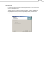
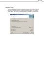
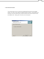
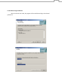
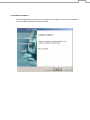
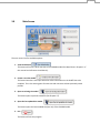
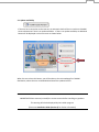
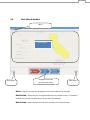
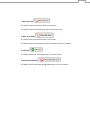
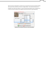
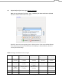
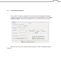
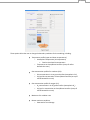
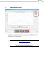
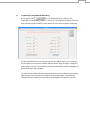
User Manual
Draft Version
June 2010
1
Table of Contents
1.0 Introduction ................................................................................................................................. 2
2.0 Installation Guide ......................................................................................................................... 3
3.0 Main Screen ............................................................................................................................... 10
4.0 Main Wizard............................................................................................................................... 12
5.0 Site Properties Panel .................................................................................................................. 15
6.0 Cover Editor Panel ...................................................................................................................... 19
7.0 Weather Simulation Panel .......................................................................................................... 35
8.0 Final Result Screen ..................................................................................................................... 38
Appendices ...................................................................................................................................... 51
2
1.0
Introduction
CALMIM (CAlifornia Landfill Methane Inventory Model) is a field-validated, 1-dimensional transport
and oxidation model that calculates annual methane emissions for individual California landfill sites
based on the major processes that control emissions:
•
Surface area and properties of the daily, intermediate, and final cover materials,
The % of surface area for each cover type with engineered gas recovery, and
Seasonal methane oxidation in each cover type as controlled by climatic factors.
The driving force for emissions is the methane concentration gradient through each cover type coupled
with dynamic soil moisture and temperature profiles which control methane transport and microbial
methane oxidation rates over a typical annual cycle. CALMIM is an IPCC (Intergovernmental Panel on
Climate Change) Tier III methodology for methane emissions from solid waste disposal sites based on a
“validated, higher quality” model (IPCC, 2006).
Based on 2.5-cm (1 inch) depth increments and 10-min time steps, CALMIM calculates daily methane
emissions on an areal basis for each individual cover (g CH4 m-2 d-1). The daily emissions are summed to
provide annual totals for each cover and for the site as a whole for a typical annual cycle (kg CH4 yr-1).
The climate-related factors (meteorology and soil microclimate) are automatically accessed based on
site location and the physical properties of the cover materials. The CALMIM model is intended to be
user-friendly with a series of input boxes to enter basic information on the areas and properties of each
daily, intermediate, and final cover material, as well as the % surface area for each cover type with
engineered gas recovery (either vertical wells or horizontal collectors).
Unlike previous inventory models for landfill methane emissions, CALMIM does not rely on a multicomponent first order kinetic, or first order decay (FOD), model for methane generation based on the
annual quantity and composition of landfilled waste. Published literature over the last decade has
indicated that, on a site-specific basis, the previous reliance on first order kinetic models for landfill
methane generation as a predictor for emissions needs to be replaced by an improved, more
scientifically-robust methodology for the following reasons:
The high uncertainty of theoretical first order kinetic models assuming homogeneous
waste and hypothetical decomposition rates in heterogeneous landfill settings (IPCC,
2006);
The complexity of methane pathways at individual sites (recovery, emissions, oxidation,
lateral migration, internal storage) where, especially at sites with high rates of
recovery, modeled generation cannot be related to measured emissions (Spokas et al.,
2006; Bogner and Spokas, 2010).
The need for a methodology which can be field-validated directly for emissions (Note:
previous “validation” of first order kinetic models for inventory purposes was based on
recovery, not emissions (e.g., Van Zanten and Scheepers, 1994; Peer et al., 1993; Scharff
and Jacobs, 2006; Thompson et al., 2009).
3
CALMIM is JAVA-based, freely available to users, and is intended to be the first step in the development
of improved science-based, field-validated models for landfill methane emissions which can be applied
internationally to calculate site-specific emissions inclusive of seasonal methane oxidation. The
development of CALMIM during 2007-2010 included a review of the technical literature; discussions
with California state agencies regarding California landfill cover materials and gas recovery practices;
decisions regarding the CALMIM conceptual framework including use of existing globally-validated U.S.
Dept. of Agriculture (USDA) models for climate and soil microclimate (Global TempSIM, Global RainSIM,
SOLARCALC, STM2); intensive supporting laboratory studies addressing methane oxidation in California
landfill cover soils; field validation over a 2-yr period at two California landfills (Marina and Scholl
Canyon); and limited field validation at 3 additional California landfills (Lancaster, Kirby Canyon, TriCities) through cooperation with an ongoing Waste Management, Inc./U.S. EPA project which is
developing optical remote sensing (ORS) techniques for field measurement of emissions.
The project team consisted of
J. Bogner (Landfills +, Inc., Wheaton, IL and University of Illinois, Chicago)
K. Spokas (USDA-ARS, St. Paul, MN), and
J. Chanton (Florida State University, Tallahassee, FL).
This project was supported by the California Energy Commission (CEC) Public Interest Energy Research
(PIER) Program [Grant No. 500-05-039] (G. Franco, Program Manager). We gratefully acknowledge the
support of Guido Franco, PIER program manager, and many individuals at the Los Angeles County
Sanitation District, the Monterey Regional Waste Management District, the former California Integrated
Waste Management Board (now part of Calrecycles), and the Air Resources Board (ARB) who generously
shared their time, provided critical reviews, and facilitated data needs for this project. In addition, we
are grateful to Waste Management, Inc. for sharing field data from their Lancaster, Kirby Canyon, and
Tri-Cities Landfills. We also sincerely thank the following individuals for technical assistance with this
project: Martin duSaire, Nancy Barbour, Dean Peterson, Chad Rollofson, Tia Phan, Lindsay Watson,
Lianne Endo, Kia Young, Mai Song Yang, and David Hamrum. Paul Roots, and Tim Badger.
Please refer to the following journal articles and the project report for additional details...
Journal Articles:
1. Spokas, K., and Bogner, J., Limits and Dynamics of Methane Oxidation in Landfill Cover Materials,
Waste Management, 2010, in press.
2. Bogner, J., Spokas, K., and Chanton, J., Seasonal Variability of CH4, CO2, and N2O Emissions from Daily,
Intermediate, and Final Cover Materials at Two California Landfills, Environmental Science & Technology,
2010, in review.
3. Spokas, K., Bogner, J., and Chanton, J., A new field-validated inventory model for landfill CH4
emissions inclusive of seasonal soil microclimate and CH4 oxidation, Global Biogeochemical Cycles, 2010,
submitted.
Project Report:
Bogner, J., Spokas, K., and Chanton, J., CALMIM (CAlifornia Landfill Methane Inventory Model) A New
Field-Validated Greenhouse Gas Inventory Methodology for Landfill Methane Emissions, 2010, Report
submitted to the California Energy Commission.
4
2.0
Installation Guide
This section will describe the installation of the CALMIM model.
CALMIM uses the Excelsior Installer from the JET family of Java pre-compiler programs.
The program is distributed via a setup program (CALMIM-setup.exe) as shown below:
This program is available for download from (http://calmim.lmem.us) or on a distribution CD
available through the California Energy Commission (PIER).
When the user double-clicks the icon, the following initial window is displayed:
The user can use the “Install” button to use all program defaults (for file location, associations,
and directories); or the user can use the Back and Next buttons to navigate through the
installation wizard (as described in the next section) to customize the installation of the
program.
5
2.1 Installation Type
On the first screen, the user can select to install the program solely for the current user or for all
the users of the computer system.
The default option is for all users to have access to this program. This option is toggled by the
associated buttons on the form. Once the user has made the selection, the “Next” button
should be clicked to move to the next window of the installation wizard.
6
2.2 Program File Location
The next screen allows the user to alter the default file locations for the model directory (default
is shown in the Destination folder box). The user can customize this selection by pressing the
“Browse” button. After the user has selected the directory for the folder, the user should press
the “Next” button for the next panel in the installation wizard.
7
2.3 File Extension Association
The next panel allows the user to associate the CALMIM profile filenames with the CALMIM
program. This option is either enabled or disabled through the checkbox. The advantage to this
association is that if the profile filename is double clicked, this will cause the computer to open
the CALMIM model. Selecting “Next” takes the user to the next panel.
8
2.4 Installation Progress Window
After the selections are made, the program will be installed according to the selected
preferences.
9
2.5 Installation Completed
The following dialog box is shown once the installation is completed. The user can immediately
start the model by leaving the checkbox enabled.
10
3.0
Main Screen
The main screen has five available options:
1. View Introduction
This button will access a brief overview of the CALMIM model (less detail than in Chapter 1 of
this manual and references cited therein).
2. Create a new site model
This button launches a new input wizard to collect information on the landfill site to be
modeled. This is the starting point for new sites and new users without previously saved
profiles.
3. Open an existing site model
This button opens a previous saved file (See Chapter 4.?)
4. Open the last updated site model
This button opens the last modeled site (last run) of the CALMIM model.
5. Exit
This button will exit the program.
11
3.1 Update availability
If the user has a connection to the internet, an automatic check will be run each time CALMIM
starts to determine if there is an update available. If there is an update available, an additional
button will be displayed on the main menu as shown below:
When the user selects this button, you will be taken to the main webpage for CALMIM
distribution, where the user can download and install the updated version.
Note:
IMPORTANT! Please remove (uninstall) the current version before installing any updates.
This warning will also be displayed by the installer program.
[Please see Installation Guide (Section 2) for further information]
12
4.0
Main Wizard Window
Menu
Panel Display
Back Button
Navigation Status Bar
(Current panel shown)
Next Button
Menu – displays the menu for the program, which is described on the next page.
Back button – Allows the user to navigate backwards in the wizard screens.
This button is
enabled once the user has advanced to the next panel (Cover Editor).
Next button – Allows the user to move to the next panel in the wizard screens.
13
Navigation status bar – Displays the current page of the wizard (in red) as well as where
the user is in the panel order.
Menu:
Menu Options:
New –
Opens a new site
Open Site –
Opens dialog box to open a previously saved site. The CALMIM profile files are saved
with a *.CMM extension.
Save Site –
Opens dialog box to save current site profile file (.CMM).
14
Mode –
This option allows the user to select the basic or advanced user levels. The advanced
mode is used to toggle whether the irrigation editor is displayed in the Weather display
panel (see Section 7). This is the sole feature that is automatically? enabled or disabled
with this option. Other advanced options are discussed in Section 6?.
15
5.0
Site Properties Panel
Required information about the landfill site to be modeled is entered on this panel.
Inputs include a site name, its latitude & longitude, and the area of the waste footprint. All of
this input information is required for each site.
5.0.1
Latitude
The latitude of the site is entered in this text box. The latitude is positive for North of the
equator and negative for locations South of the equator. For example, the latitude for Sydney
Australia (33o 55’ South) would be entered as -33.92 and for Chicago, IL (USA; 41o 51’ North)
would be +42.85.
5.0.2.
Longitude
The longitude of the site is entered in this textbox. East is entered as positive values and West
longitudes are negative values. For example, the longitude for Sydney, Australia (151o 17’ East)
would be entered as +151.28 and for Chicago, IL (USA; 87o 41’ West) would be -87.68.
5.0.3. Site Waste Footprint
This is the total area of the waste footprint in acres, which represents the area of the site where
waste is currently or has been historically deposited. This is NOT the total size or permitted area
of the landfill site.
16
5. 1
SWIS Database Search
By entering a part of the name in the site name box and then by pressing “Enter” or the search
button, the program will attempt to locate the site in the California SWIS (Solid Waste
Information System) database included with the CALMIM model
(http://www.calrecycle.ca.gov/SWFAcilities/Directory/).
The model will display a pop up box:
The user can select the site from the pull-down box and then click on the “Select Site” button
. The program will automatically populate the corresponding text boxes with
the latitude, longitude, and waste footprint (if available in SWIS records). The user will then be
returned to the main wizard.
If none of the listed sites are the desired site, please select “Cancel” and the program will return
to the wizard. At this point, the user could either modify the search or continue by manually
entering the required data.
If the site is not found, the model will display a warning box notifying the user that the site was
not located in the database.
17
5.2
Map Options
The map is set for locations in California (see Map Panel in Site Information panel above).
However, if the user wished to enter a location outside of California, the user can select the
“View World Map” button:
This button is located at the bottom of the Location Map panel as shown below.
If this button is selected, the model will change to the world view:
18
To return to the California map, the user can select the
button. NOTE:
even though the model will run for non-California locations, the current version of the CALMIM model
has been field-validated only for California.
5.2.1 Location Selection from Maps
By clicking any location on the map, and then correspondingly clicking the button:
The user can populate the latitude and longitude locations from the world map (or California
map) into the respective text boxes for latitude and longitude.
For non-California locations, the user must enter a site name and the corresponding waste
footprint (site footprint), before continuing to the next panel.
19
6.0
Cover Editor Panel
This panel allows the user to customize up to 10 different covers for any site.
20
6.1
Cover Tabs
There are two main buttons to add or delete covers from the model:
1. Add New Cover button
The user should use this button to add a new cover to the model. The program will prompt
the user for a name for the cover as shown below:
The name should be descriptive enough for the user to identify the cover in the output, for
example “Intermediate1” or similar. This new cover will then appear as a tab as shown in
the figure below.
21
The user can switch between cover types by clicking on the respective tabs for the various
covers.
Renaming Cover Tabs
By double clicking on the tabs, the user can rename the various cover tabs. This will
highlight the tab to allow a new cover name to be entered. Up to 10 different covers can be
entered per model run.
2. Remove Current Cover
This button will remove the currently selected cover tab. The model will not allow the user
to delete the last tab as one model tab is required for the model to run. Before deleting any
cover, the model will confirm the delete with the user using the dialog box shown below:
22
The name of the selected cover will appear in the dialog box in place of Interemdiate1 in the
example dialog above.
23
6.2
“Cover Details” Section of Panel
6.1.1
Cover Type
These 3 buttons allow the user to select the basic cover type. Please note that this
selection determines default boundary gas concentrations, default temperature profiles,
and maximum methane oxidation rate for each cover type (See Appendix A).
There is also the selection for a “Custom” cover type, which is selected by checking the
Custom checkbox:
24
When the custom cover type is selected the model displays the “Custom boundary conditions”
button:
The features of this button are described later (section 6.5)
6.1.2
Coverage Percentage
This slider bar allows the user to specify the percentage of the waste footprint that this
cover represents. For example, as shown in the figure below, the percent coverage for
different representative areas of the hypothetical landfill:
Daily
Cover Area
Final Cover Area
Total Landfill Footprint
20%
Coverage
6.1.1
Cover Properties
a. Organic matter (slider bar)
Total Landfill Footprint
2%
Coverage
Total L
Foot
25
This selection controls the amount of organic material that the model uses for
calculation of the soil properties (see below). High Organic material cover materials
would be those amended with sewage sludge, compost, wood chips, or other organic
wastes. This slider bar from Low to High represents a range of 0 to 5% organic matter.
b. Gas Recovery System Information
If a gas recovery system is present, the user should select the Gas Recovery checkbox,
which will enable the gas recovery slider bar as shown below:
NOTE: This percentage is NOT the estimated efficiency of the gas recovery system.
Instead, this percentage represents only the areal coverage of any gas recovery system
for a particular cover type.
The user should select the percent of the area for this cover type which has a gas recovery
system in place (vertical wells, horizontal collectors, or combination). Some examples are given
below.
To LFG
recovery
system
33% Gas Recovery Coverage
To LFG
recovery
system
100% Gas Recovery Coverage
To LFG
recovery
system
50% Gas Recovery Coverage
26
c. Vegetation Present
If there is vegetation present on the cover type, then the user should select the
“Vegetation Present” checkbox, which will enable the vegetation present scroll bar.
The user should use the scroll bar to enter the approximate average annual vegetation
coverage for this cover type. This is an estimate of the percentage of the surface area
which is typically covered by vegetation.
27
6.2
Cover Editor
6.2.1 Highlighting a layer in the cover editor
To highlight a layer:
Position the mouse over any element (layer number, cover material, or thickness) and press the
mouse button. The selected layer will be highlighted in blue as shown in the figure below (layer
#2  6 inch sand layer is selected):
28
1. Move Layer Up
This option is only functional with two or more layers.
This button moves the selected layer closer to the surface (up).
2. Move Layer Down
This option is only functional with two or more layers.
This button moves the selected layer closer to the base of the cover (down).
3. Add Layer
This option adds a new layer (default layer is 6 inches of clay).
4. Remove Selected Layer
This button removes the selected (highlighted) layer in the cover editor.
29
6.2.2 Cover Layer Editor
Once a layer is highlighted (see Section 4.2.1), the layer editor becomes visible for that
respective layer.
Note: the title bar of the editor indicates which layer you are currently editing. See circled area
in figure below.
Once the layer editor is enabled by highlighting the respective layer, the user makes a selection
among the 12 USDA soil texture classifications or among 21 other alternative choices through
the pull-down combo box. The alternative choices are alternative daily cover (ADC) materials
and non-soil materials, including geomembranes. The model will display either the section of
the textual triangle selected (USDA soil types) or a representative picture of the cover material
selected. See Appendix A for the physical properties (default values) for the various materials.
(Combo box for material selection is shown expanded)
30
After the material is selected for a particular layer, the thickness of the layer should be specified
with the pull-down combo box as shown in the figure below. The maximum thickness for an
individual layer is 100 inches (254 cm). Some of the specialized materials have a fixed thickness,
so the user will not be able to select a different value for thickness (e.g. geomembranes).
(Combo box for thickness selection is shown expanded)
31
6.4
Default California final cover types (only for Final Cover)
When the user selects the “Final cover” type, an additional pull-down combo box is displayed
with the 5 default California final cover types.
Details for these final cover types are given in Table 6.1 below. If the cover conditions deviate
from these values, each layer should be entered individually as discussed above, rather than
selecting the default design.
Table 6.1. Settings for Default Final Cover Types
Layer
CCR Title 27
Geosynthetic Clay
(without geomembrane)
Geosynthetic Cover
(with geomembrane)
Water Balance
(Vegetation Surface)
Water Balance
(rock armored)
1
Loam
(12 inches)
Loam
(12 inches)
Loam
(12 inches)
Loam
(12 inches)
Rocks/Boulders
(6 inches)
2
Clay
(12 inches)
Clay
(40 inches)
HDPE
geomembrane
(1 inch*)
Silty Clay Loam
(36 inches)
Loam
(12 inches)
3
Silty Clay
Loam
(24 inches)
Silty Clay Loam
(12 inches)
Silty Clay Loam
(24 inches)
Vegetation
(%)
50
50
50
Notes: * indicates the required minimum thickness in the program
Silty Clay Loam
(36 inches)
50
0
32
6.5
Custom boundary conditions
If the “Custom” checkbox is selected, the user can override the existing default boundary
conditions for a given cover type (daily, intermediate, or final; See Appendix 1). The “Custom
Boundary Conditions” button will be displayed in the cover editor panel as shown below:
When the user clicks on the “Custom Boundary Conditions” button, the dialog box below is
displayed.
33
These options allow the user to change the boundary conditions for the modeling, including:
Temperature profile (upper and lower temperatures)
o Atmospheric temperature (Air temperature)
 Fixed or simulated air temperature
o Temperature at Cover/Waste interface (at top of refuse
beneath the cover)
Gas concentration profiles for methane (CH4):
o CH4 concentration in air at ground surface (atmospheric CH4)
o Soil gas CH4 concentration at Cover/Waste interface (at top of
refuse beneath the cover)
Gas concentration profile for oxygen (O2):
o O2 concentration in air at ground surface (atmospheric O2)
o Soil gas O2 concentration at Cover/Waste interface (at top of
refuse beneath the cover)
Maximum CH4 oxidation rate
Bottom moisture conditions
o Saturated or free drainage
34
Temperature profile (upper and lower temperatures)
The upper limit can be a user-selected constant value (“User Selected”) or the
variable air temperature from the weather simulation. The latter is
recommended.
The lower boundary is held constant at the designated set point.
Gas Concentrations:
The concentrations of methane and oxygen are both specified (in percent by
volume) for the upper boundary (concentration in atmosphere) and the lower
boundary (soil gas concentration at the base of cover – the cover/waste
interface)
Bottom Moisture Conditions:
The saturated condition at the bottom of the cover is the default boundary
condition, since the field state for the waste/soil interface is typically saturated
due to the high humidity of the landfill gas.
However, the user could change this to a free drainage condition.
The upper moisture condition is controlled by the simulated weather (either
evaporation or precipitation) and cannot be changed by the user.
35
7.0
Weather Simulation Screen
The weather simulation panel displays the results of the weather simulation for the site as
individual graphs. Each graph can be viewed by selecting the respective tab at the upper right
side of the screen (see circled tabs above).
The graphical libraries used in this program are from JFreeChart
(http://www.jfree.org/index.html)
and the user is encouraged to visit the webpage
(http://www.jfree.org/jfreechart/api/javadoc/index.html)
for further information on the available graph options.
36
7.1
Irrigation Info Tab (Advanced Mode Only)
The ”Irrigation Info”
is only displayed when the user is in the
“Advanced” mode (See Menu Options – Section 4). The irrigation tab allows the user to
enter monthly irrigation totals (in mm of water) for sites where irrigation is practiced:
The user should input the total monthly amounts of irrigation water (in mm of water)
for the month in the respective textbox, and then select “Apply Changes” to apply the
new irrigation amounts. The model will display the new monthly totals and highlight (in
green) those which were updated.
The other button (“Generate New Precipitation Data”) will erase the previous irrigation
data so that the user can generate a new set of precipitation data. This should be
selected if the user made a serious mistake in entering data and wants to start over.
37
7.0
Model Calculation Screen
While the model is calculating the following screen is displayed:
This dialog box displays progress for model calculations for the current cover, along with
the estimated time remaining for that cover. It is important to note that the time
remaining only applies to the current cover and not to the entire model run.
The progress bar at the top indicates model progress for the total number of covers
entered by the user. The abort calculation button allows you to abort the run and exit
the program. No intermediate data from the calculations are stored. The model could
be restarted by using the “Open the last updated site model” (page 3) to restart the
model.
38
8.0
Final Results Screen
After the model has completed the calculations, the final screen is displayed:
A number of different graphs can be individually viewed for each cover type by selecting
the tabs at the upper right side of the screen. Each of these graphs will be described
individually in the following pages. The user can navigate through the various cover
types by selecting the corresponding tab along the top of the screen panel. In addition,
there is a “Site Report” tab, which summarizes the results for the site.
In addition, the left mouse button can be used to click and drag in order to zoom-in on
an area of interest as shown below: here the highlighted region (purple/blue) is being
zoomed to the size of the graph at the right after release of the left mouse button.
39
For each of the graphs, when the mouse is on the graph, the user can press the right
mouse button to display an option menu for the figure:
Selecting “Properties…” brings up the properties screen, where the user can change and
alter the appearance of the graphs.
The “Save as” and “Print” functions will allow any particular graph to be saved or
printed for future reference.
40
The graphical libraries used in this program are from JFreeChart
(http://www.jfree.org/index.html)
and the user is encouraged to visit the webpage
(http://www.jfree.org/jfreechart/api/javadoc/index.html)
for further information on the available graph options.
41
-Predicted Surface Methane Emissions for a Selected Cover
This graph displays the variable surface emissions (10-min. time steps) for a typical
annual cycle (365 days) both without methanotrophic methane oxidation (black line)
and with methane oxidation (red line) included in the calculations. CALMIM calculates
these separately so that the effect of oxidation (difference between the two plots) can
be readily seen on this graph.
This graph clearly shows the high variability in emissions calculated by the model as a
result of the variable soil moisture and temperature within the cover soil and how this
impacts both gaseous diffusion and microbial methane oxidation. These variable
impacts can be seen in additional detail in the following graphs.
42
-Predicted Percent Oxidation for this Particular Cover
This graph illustrates the calculated percent oxidation as a result of the variable
temperature and soil moisture conditions in the landfill cover materials. The percent
oxidation is calculated from the difference between the two methane emission plots
(with and without oxidation) shown above. This graph plots the percent of emissions at
each time step “without oxidation” which is represented by the emissions at that time
step “with oxidation.” Thus, this graph shows the net total effect of comparing surface
emission values with and without oxidation.
43
-Predicted Temperature of each Node
This graph illustrates the surface, mid and bottom node soil temperatures at these 3 respective
depths for the selected cover.
44
-Predicted Soil Moisture (volumetric) of each Node
This graph display the surface, mid and bottom node results for volumetric soil moisture at
these 3 respective depths for the selected cover.
45
-Predicted Air-Filled Porosity of each Node
This graph illustrates the surface, mid and bottom node alterations in air-filled porosity
at these 3 respective depths for the selected cover. Air-filled porosity changes as a
function of the fluctuating soil moisture conditions.
46
- Oxygen Concentration within each Node
This graph illustrates the surface, mid and bottom node results for soil gas oxygen
concentrations (V%) at these 3 respective depths for the selected cover. This value is an
indication of the aeration status of the cover soil.
47
- Methane Concentration within each Node without Methane
Oxidation
This graph illustrates the surface, mid and bottom node results for soil gas methane
concentration (V%) without methane oxidation at these 3 respective depths for the selected
cover.
48
- Methane Concentration within each Node with Methane Oxidation
This graph illustrates the surface, mid and bottom node results for soil gas methane
concentration (V%) with methane oxidation at these 3 respective depths for the
selected cover. methane concentrations with methane oxidation. Note the drastic
difference in methane concentrations between the “with” and “without” methane
oxidation scenarios. Also note the highly variable methane concentration in the middle
layer of this particular cover.
49
- Percent Oxidation within each Node
This graph illustrates the total methane oxidation rate per node (in units of
g CH4 m-2 day-1) at the same 3 respective depths for the selected cover. Note that this is
calculated separately for each node and is NOT the methane surface emissions.
50
- Depth Profile of Methane Oxidation
This graph illustrates the percentage of time (over an annual cycle) that each node over
the total depth of a selected cover is capable of oxidizing methane.
51
Appendix A
Default boundary conditions for different cover types
Table A1. Default conditions for selected cover types.
Cover Type
Lower Temperature Boundary
Condition
(oC)
25
Lower Methane Boundary
Condition
(% vol)
0.30
Lower Oxygen Boundary
Condition
(% vol)
5
Intermediate
35
45
1
Final
40
55
0
Daily
52
53
Appendix B
Default Material Properties in Model
Soil Materials
SAND
SANDY CLAY
LOAMY SAND
SANDY LOAM
SILTY LOAM
LOAM
SANDY CLAY LOAM
SILTY CLAY LOAM
CLAY LOAM
SILTY CLAY
CLAY
SILT
Rocks - Pebbles
Rocks - Boulders (large)
ADC Foundry Sands
ADC Dredged Materials
ADC Ash
ADC Contaminated Soils (clay)
ADC Contaminated Soils (sand)
ADC Contaminated Soils (general - loam)
ADC Tire Shreds [small <2 in (50 mm)]
ADC Tire Shreds [large >2 in (50 mm)]
ADC Wood Chips (all)
ADC sludge
ADC Energy Resource Exploration and Production Wastes
ADC Composted Organic Materials
Non-Soil Materials
Geomembrane (HDPE)
Geomembrane (LDPE)
Geomembrane (EDPM)
Geotextile (woven)
ADC Spray Applied Cement Products
ADC Spray Applied Foams
ADC Temporary Tarp
Sand (%)
Silt (%)
Clay (%)
Soil ? Bulk Density (g/cm3) SatConductivity (kg/m3)
Volunteric Moisture (33 kPa)
Volumetric Moisture (1500 kPa)
Beta (Campbell) Total Porosity (33 kPa)
93.6
93.6
82.74
65.6
21.8
42.9
60.1
9
34.7
9.3
10
7.96
93.6
95.6
90
7.96
21.8
10
90
42.9
90
90
90
10
42.9
42.9
3.06
3.06
9.66
22.5
62.7
39.5
11.3
55
30.3
43.89
25
63.62
3.06
2.06
5
63.62
62.7
25
5
39.5
5
5
5
80
39.5
39.5
3.34
3.34
7.6
11.9
15.5
17.6
28.6
36
35
46.81
65
5.41
3.34
2.34
5
5.41
15.5
65
5
17.6
5
5
5
10
17.6
17.6
true
true
true
true
true
true
true
true
true
true
true
true
true
true
true
true
true
true
true
true
true
true
true
true
true
true
1.63
1.44
1.58
1.53
1.28
1.40
1.47
1.24
1.35
1.28
1.26
1.16
1.63
2.01
1.63
1.16
1.28
1.26
1.63
1.40
1.08
1.63
1.08
1.20
1.40
1.40
0.002703
0.000176
0.001760
0.000763
0.000137
0.000292
0.000356
0.000052
0.000125
0.000031
0.000034
0.000106
0.002703
0.003100
0.003703
0.000106
0.000137
0.000034
0.003703
0.000292
0.051300
0.003703
0.081300
0.001060
0.000292
0.000292
0.091
0.231
0.116
0.139
0.276
0.223
0.2
0.321
0.264
0.312
0.351
0.332
0.091
0.071
0.1
0.332
0.276
0.351
0.1
0.223
0.19
0.1
0.22
0.452
0.223
0.223
0.039
0.113
0.051
0.062
0.125
0.102
0.095
0.151
0.125
0.15
0.172
0.149
0.039
0.019
0.04
0.149
0.125
0.172
0.04
0.102
0.06
0.04
0.06
0.15
0.102
0.102
2.01
10.21
2.86
4.29
6.86
6.26
7.42
10.36
8.94
13.00
14.20
6.72
2.01
2.01
3.00
6.72
6.86
14.20
3.00
6.26
2.00
3.00
2.00
8.70
6.26
6.26
0.386
0.455
0.402
0.422
0.518
0.474
0.445
0.532
0.489
0.517
0.524
0.564
0.386
0.245
0.39
0.564
0.518
0.524
0.39
0.474
0.51
0.39
0.33
0.564
0.474
0.474
10
10
10
10
10
10
10
25
25
25
25
25
25
25
65
65
65
65
65
65
65
false
false
false
false
false
false
false
1.26
1.26
1.26
1.26
1.26
1.26
1.26
0.000034
0.000034
0.000034
0.000034
0.000034
0.000034
0.000034
0.351
0.351
0.351
0.351
0.351
0.351
0.351
0.172
0.172
0.172
0.172
0.172
0.172
0.172
14.20
14.20
14.20
14.20
14.20
14.20
14.20
0.524
0.524
0.524
0.524
0.524
0.524
0.524
54
Appendix C
Geomembrane notes
Average Ksat for a HDPE geomembrane is around 4 x 10-13 m/sec (Narejo and Memon, 1995;
Giroud and Badu-Tweneboah, 1992). For the geomembrane node (1 inch thick = 2.54 cm), the
effective hydraulic conductivity is calculated by the following formula:
MISSING FORMULA
Add reference list, including references in text...