Download - University of Mississippi

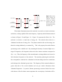
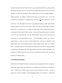
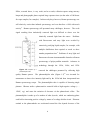
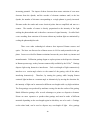
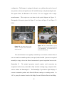
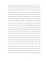
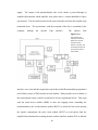
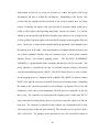
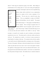
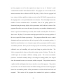
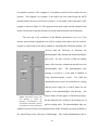
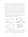
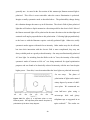
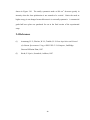
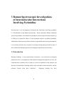
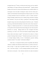
UPGRADE OF A RAMAN SPECTROMETER WITH
MODERN COMPUTER CONTROL AND DATA
ACQUISITION FOR STUDIES OF HYDROGEN
BONDING IN PYRIMIDINE
by
Austin Archie Howard
A thesis submitted to the faculty of the University of Mississippi in
partial fulfillment of the requirements of the Sally McDonnell Barksdale
Honors College
Oxford
May 2009
Approved by
Advisor: Professor Nathan Hammer
Reader: Professor Gregory Tschumper
Reader: Professor Susan Pedigo
ACKNOWLEDGEMENTS
Many people in the Department of Chemistry and Biochemistry here at the University of
Mississippi were of great assistance during the work presented in this manuscript. I
would like to thank the members of the Keith Hollis, Daniell Mattern, Walter Cleland,
Takashi Tomioka, and Susan Pedigo research groups for the donation of some of the
chemicals used in these experiments. I would like to thank Dr. Susan Pedigo for the
extended loan of a circulating water bath, without which the Raman spectrometer could
acquire no data. I would like to thank Dr. Maurice Eftink for taking the time to teach me
how to use his high pressure apparatus. I would like to thank the research group of Dr.
Gregory Tschumper for assisting in matters of computations. I would also like to thank
the members of my research group for always being of assistance. Lastly, I would like to
thank my advisor Dr. Nathan Hammer for allowing me a position in his laboratory as
well as a worthwhile project to fulfill this thesis requirement.
ii ABSTRACT
AUSTIN ARCHIE HOWARD: Upgrade of a Raman Spectrometer with Modern
Computer Control and Data Acquisition for Studies of Hydrogen Bonding in Pyrimidine
(Under the direction of Dr. Nathan Hammer)
The restoration of a Cold War era high resolution Raman spectrometer to working order
as well as its control and data acquisition upgrade using a Labview program authored for
this purpose are discussed.
The restored Raman spectrometer was used in an
investigation of intermolecular interactions involving pyrimidine.
Following in this
manuscript are three chapters. The first chapter is a brief description of the history and
theory of Raman spectroscopy as well as some details of the instrumentation used in
Raman spectroscopy. The second chapter contains technical details of the restoration and
upgrade of the high resolution Raman spectrometer. The third chapter contains data and
analysis for the investigation of intermolecular interactions involving pyrimidine,
including the investigation of weak hydrogen bonds by Raman spectroscopy of liquid and
crystalline pyrimidine at varying pressures up to 30000 psi and strong hydrogen bonds in
binary mixtures of pyrimidine and seven different molecules. The position of the ν1 peak
in the Raman spectrum corresponding to pyrimidine’s ring-breathing mode was used as
the marker to monitor the degree of hydrogen bonding and species involved.
For
mixtures of water, other peaks in the Raman spectrum were found to shift as well when
the concentration of water is increased.
iii TABLE OF CONTENTS
1. History, Theory, and Instrumentation……………………………………………………..1
1.1 Light-Matter Interaction………………………………………………...……………1
1.2 The Raman Effect……………………………………………………………..……..4
1.3 Instrumentation……………………………………………………………………....8
1.4 References…………………………………………………………………………..12
2. Upgrade of a High Resolution Cold War Era Raman Spectrometer
for Modern Data Acquisition and Control…………………………..….....…………..…14
2.1 Ramanor HG2-S Raman Spectrometer………………………………………..…...14
2.2 The Restoration…………………………………….………………………………19
2.3 The New Experimental Setup………………….…………………………………..26
2.4 References………………………………………………………….………………30
3. Raman Spectroscopic Investigations of Intermolecular Interactions Involving
Pyrimidine………………………………………………………………...………..………31
3.1 Introduction……………………..……………………………………………….…31
3.2 Experimental.…………………………...…………………………………………35
3.3 Results and Discussion….……………………………...…………………………36
3.4 Conclusion…………………………….…………..………………………….……49
3.5 References………………………………….……………………………….…….50
iv 1 History, Theory, and Instrumentation
Spectroscopy is the study of the interaction of light and matter.1 The measurement of this
interaction can reveal a wide range of chemical and physical behavior in systems being
studied. Raman spectroscopy exploits the Raman Effect, the inelastic scattering of light
by molecules. Following is a brief introduction to the interaction of light and matter, first
with a description of light scattering and then with a description of the Raman Effect and
its relationship to the vibrational energy of molecules. This background information
precedes a short history of Raman instrumentation containing pertinent technical details.
1.1 Light-Matter Interaction
When light is incident on an atom or molecule, there are two possibilities for interaction.
First, a photon with an energy exactly matching that of a vibrational, electronic, or
rotational energy level transition can be absorbed by the atom or molecule.
This
absorption promotes the system to a higher energy level. For photons not of the correct
energy to be absorbed, scattering can occur. The elastic scattering of photons was
described in the 19th century, an effect now known as Rayleigh scattering.2
Lord
Rayleigh showed the relationship between scattering power and wavelength and why this
causes the blue color of the sky. Rayleigh scattering occurs by a process in which the
1 oscillating electric field of light incident on a molecule induces a dipole moment in the
molecule by separating positive and negative charge density. Because the electric field
oscillates sinusoidally, the induced dipole moment oscillates with the same frequency.
Since electric dipoles produce electric fields, this dipole oscillation produces a new
electric field oscillating with the same frequency as the incident light. Oscillating electric
fields induce oscillating magnetic fields, and thus new light of the same frequency as the
incident light has been produced, emanating in all directions from the molecule. This
scattering process is termed elastic because the energy of the incident light is equal to the
energy of the scattered light following from the fact that energy is related to frequency by
Planck’s constant (Eqn. 1).
(1)
We can imagine this process with a classical picture of the oscillating dipole described
above. In a linear dielectric material, the magnitude of an induced dipole is given by
Equation 2.
(2)
In Equation 2, p represents the magnitude of the induced dipole, α is the polarizability of
the material, and E is the magnitude of the electric field responsible for the induced
dipole. For electromagnetic radiation, we know that the electric field has the form
cos
where Eo is the magnitude of the electric field, ω is the angular frequency
(the frequency f in hertz multiplied by 2π), and t is the time. It is trivial, then, to
substitute the correct form of the electric field in an incident light wave into Equation 2 to
obtain Equation 3, an expression for the frequency of the oscillating dipole when light
undergoes Rayleigh scattering.
2 cos
(3)
When a photon is inelastically scattered (Raman scattered), the scattered radiation
has a different energy and thus frequency than the incident radiation. Inelastic scattering
of photons was first discovered in 1923 when Arthur Holly Compton found that X-rays
were shifted to longer wavelengths in collisions with electrons.3
In 1923, while
investigating theoretically the dispersion of electromagnetic radiation using a quantum
model of light, Adolf Smekal showed that scattered monochromatic light would have
components at higher and lower frequencies in addition to the elastically scattered
component, thus theoretically predicting inelastic scattering. However, this and other
contributions to the discussion of dispersion at the time did not influence C.V. Raman in
his work.4 Raman had been investigating the scattering of light since the early 1920’s in
order to disprove Rayleigh’s idea that the blue appearance of the sea was due only to the
reflection of the sky.4
Raman was also led by similar interests to experimentally
investigate how light is scattered in liquids and crystals. Raman’s discovery of the effect
now bearing his name took place during his attempts to find the optical analog of the
Compton scattering of X-rays.4
Raman’s setup used a telescope to focus sunlight onto various samples. A colored
filter was used to illuminate the samples with monochromatic light, and a spectroscope
was used to visually detect a change in the color of the scattered radiation. The effect
was first termed by Raman and his assistants a “feeble fluorescence,” referring to an
optical process resulting from electronic relaxation, but a change in polarization of the
scattered light distinguished this effect from fluorescence.3 The effect was very weak
(approximately 1 in 108 photons are scattered this way), but using long exposure times,
3 Raman was able to collect the spectra (on photographic plates in those days) of sixty
different liquids and vapors. These spectra first appeared in the Indian Journal of
Physics5 along with his articles. Because Nature6,7 had not published Raman’s spectra
with his articles, he sent copies of the Indian Journal of Physics paper to two thousand
scientists in France, Germany, Russian, Canada, and the United States.4 Raman realized
as others did that the spacing of the lines in spectra he collected was equal to the infrared
frequencies of the molecules represented by the spectra.4 The terms Raman Effect and
Raman lines were coined by 1929,4 and physicists and chemists all over the world began
to collect Raman spectra to investigate the vibration and rotation of molecules and verify
quantum theories.3
1.2 The Raman Effect
A simplified explanation of the Raman Effect and its relation to molecular vibrations
follows. According to Equation 2 above, the induced dipole moment in a molecule is
equal to the product of the polarizability and the applied electric field. Molecules are
constantly vibrating at any temperature above 0 K.
For a homonuclear diatomic
molecule, we can write the nuclear displacement from the equilibrium position as
Equation 4.
cos
(4)
Equation 4 is a result of modeling the two atoms as two masses connected by a spring.
That is, the atoms are subject to a restoring force directly proportional to displacement
from equilibrium. Here, ωv is the angular frequency of the vibration. These vibrations
4 cause a change in electron density, and as a result, the polarizability is not accurately
represented by a static variable but as a function of nuclear position (Equation 5).
(5)
This series can be truncated at the term linear in qo for small amplitudes of vibration.
Now, Equation 3 can be written with Equation 5 substituted for the polarizability.
cos
cos
(6)
cos
(7)
Now, we substitute the expression for q (Equation 4).
cos
cos
Lastly, applying the trigonometric identity cos cos
cos
cos
,
we obtain a classical theory describing Raman scattered light.
cos
1
2
cos
(8)
cos
We can see from the above equation that the dipole induced by light interacting with the
vibrating diatomic molecule is oscillating with frequency ω, the frequency of the incident
radiation corresponding to the Rayleigh scattered light.
Also, the dipole contains
components oscillating with frequencies ω+ωv and ω-ωv. The result is that the induced
dipole is emitting light with frequencies greater than or less than the incident light by an
amount equal to the frequency of vibration. An energy level diagram for each situation is
shown in Figure 1.1.
5 Figure 1.1 An energy Virtual State Excited Vibrational State Vibrational Ground State (a) (b) diagram showing the vibrational transitions resulting a) Rayleigh scattered light and Raman scattered light of the b) Stokes and c) anti‐Stokes lines. (c) When light is Rayleigh scattered, the molecule is excited to a virtual excited state
and relaxes, creating a photon of the same frequency. Light may also be Raman scattered
as shown in Figure 1.1b and Figure 1.1c. Figure 1.1b represents the Stokes line. The
molecule is excited to a virtual state of energy
vibrational excited state of energy
. The molecule then relaxes to a
. The photon created in this case has energy less
than the exciting radiation by an amount
. This is the property that makes Raman
spectroscopy such a valuable tool. By measuring the intensity of scattered light over a
range of frequencies, the frequencies observed to have intense emissions correspond to
. Thus, the frequency of the monochromatic exciting radiation can be used to
find vibrational frequencies of the molecule. The transition producing the anti-Stokes
line corresponds to a molecule in a vibrational excited state being excited to a virtual state
and relaxing to the vibrational ground state. The frequency of this scattered radiation is
greater than that of the excited radiation and can give similar information about
vibrational frequencies. In practice, Raman spectroscopy measures Stokes lines more
often because of the fact that at room temperature the vast majority of molecules will be
6 in the vibrational ground state. With more molecules to produce them, the Stokes lines
will be more intense. It is worth noting that Stokes and anti-Stokes lines are terms
originating in fluorescence spectroscopy. A fluorescence peak is predicted to be at a
lower energy than the exciting radiation producing the fluorescence and is said to have
Stokes-shifted. This process is wholly unrelated to the Stokes lines produced by the
Raman Effect, and the use of these terms has simply carried over from fluorescence
spectroscopy.
This above situation was described for a homonuclear diatomic molecule for
simplicity. For a general polyatomic molecule, the case becomes more complicated. The
vibrations are not just stretching or contraction of one bond but can be any linear
combination of what are known as normal modes. The term normal mode when applied
to molecular vibrations is characterized by the fact that each atom executes simple
harmonic motion with the same frequency, and the atoms generally move in phase.8
Normal refers to the fact that the displacements of one atom during any two different
normal modes are orthogonal, i.e. have an inner product of zero. For a molecule of N
atoms, there exist 3N-6 normal modes (or 3N-5 for a linear molecule). This number
corresponds to three degrees of freedom of motion for each atom (i.e. in the x, y, and z
directions) with the number of motions corresponding to rotation and translation of the
molecule subtracted.
As noted above, any motion of the atoms of a molecule can be
represented by an equation of motion that is nothing more than a linear combination of
the normal mode equations of motion. Each normal mode has an energy associated with
it, although the energy may be the same for two normal modes. The predicted energy for
a normal mode and often its symmetry properties are used to assign the peaks in a Raman
7 spectrum to particular normal modes. Not every normal mode will have a peak present in
the Raman spectrum, however. As noted, two normal modes may have the same energy
and then are said to be degenerate. These normal modes will not be distinguishable in a
Raman spectrum. In addition, certain normal modes are not Raman active. Notice the
second term in Equation 8 containing the derivative
as a coefficient.
If this
derivative is zero, the dipole will not have components oscillating at either of the Raman
shifted frequencies, at least to first order. Thus, no Raman scattered light will appear.
Physically, we interpret this as a change in polarization with a normal mode being a
requirement for that mode’s Raman activity. In moving from the homonuclear diatomic
case to the general polyatomic case, the induced dipole and the electric field must be
represented as three dimensional vectors.
The polarizability in this case must be
represented as a rank two tensor in three dimensions. Only one component of the
polarizability tensor must change during a normal mode for this mode to be Raman
active. Typically, modes are determined to be Raman active or inactive using symmetry
considerations of the mode and of the polarizability tensor for a certain point group. One
advantage of Raman spectroscopy is that some vibrational modes that are not infrared
active may be Raman active.
1.3 Instrumentation
Raman first used sunlight focused by a telescope as the exciting source in his experiments
along with colored filters and the human eye for detection of the effect now bearing his
name. Raman first collected spectra using a mercury lamp as the source, a prism to
disperse the scattered radiation, and photographic plates as the detectors. The Raman
8 Effect, as noted above, is very weak, and as a result, collection spectra using mercury
lamps and photographic plates required long exposure times (on the order of 180 hours
for vapor samples, for example4). In these early days, however, Raman spectroscopy was
still relatively easier than infrared spectroscopy and was therefore a field with much
activity.9 Raman spectroscopy still presented many challenges, however. The weak
signal resulting from inelastically scattered light was difficult to detect over the
elastically scattered light from the source.
Problems
with fluorescence and stray light were avoided by
extensively purifying liquid samples, for example, with
multiple distillations that required as much as three
months preparation time.9 Problems of stray light and
fluorescence became insurmountable obstacles to Raman
spectroscopy of polycrystalline materials. Advances in
technology through the 1950s, 1960s, and 1970s
Figure 1.2 Principles of a photomultiplier tube quality Raman spectra.
removed the challenges presented by collecting high
The photomultiplier tube (Figure 1.2)10 was invented for
astronomers to detect low intensity light and by the 1950s had been incorporated into
Raman spectroscopy setups. The photomultiplier tube is capable of detecting single
photons. Photons strike a photosensitive material held at high negative voltage (~ 1500V, e.g.) and cause the emission of electrons via the photoelectric effect.
The
photomultiplier is made up of a number of other dynodes, which are conducting plates
each held at increasing positive voltage by means of a voltage divider circuit. Electrons
emitted at the photocathode are accelerated toward the first dynode because of the
9 increasing potential. The impact of these electrons then causes emission of even more
electrons from the dynode, and the cascade of electrons continues until, at the last
dynode, the number of electrons corresponding to a single photon is greatly increased.
Electrons strike the anode and create electrical pulses that are amplified and sent to a
counter. The number of counts is directly proportional to the intensity of the light
striking the photocathode and is therefore a measure of signal intensity. So-called dark
counts resulting from emission of electrons without any incident light are minimized by
cooling the photomultiplier tube. There were other technological advances that improved Raman sources and
optics. The laser was first used as a Raman source in 1964 to study materials in the gas
phase. Lasers were ideal for Raman excitations because they were both very intense and
monochromatic. Diffraction gratings began to replace prisms as the dispersive elements
in Raman spectroscopy as they became commercially available by the 1950s.11 Gratings
disperse light using destructive interference. Each wavelength of light constructively
interferes at a certain angle relative to the normal of the grating with all the others
interfering destructively.
Therefore, by turning the grating while keeping Raman
scattered light incident at a constant angle or alternatively by moving the detection slit,
the intensity of light can be measured at different wavelengths with very high resolution.
The first gratings were produced by machines carving slits into the surface of the grating.
Ruled diffraction gratings offer several advantages to prisms as dispersive elements.
Prisms are more expensive to produce than gratings and must be made of different
materials depending on the wavelength region in which they are to be used.12 Gratings,
on the other hand, can be used to disperse any wavelength of light. Also, gratings
10 disperse light linearly, unlike prisms. In the 1960s interference or holographic gratings
were first developed. These gratings are produced by an interference pattern of an
intense light source varying sinusoidally in intensity along the surface of a photosensitive
material. The degraded portion of the material is then dissolved, producing grooves in a
sinusoidal pattern on the grating.
Holographic gratings began to be produced
commercially in 1972 and hold many advantages over mechanically ruled gratings in
Raman spectroscopy. Flaws in the rulings of a mechanical grating resulting from carving
one groove at a time are virtually nonexistent in holographic gratings, in which all the
grooves are formed simultaneously. Holographic gratings also reduce the amount of
stray light resulting from scattering by the grating itself.11
By the 1970s Raman
spectrometers were commercially sold with multiple holographic gratings that could
record spectra within 5 cm-1 of the Rayleigh scattered light of the laser.9
The next major advances in Raman spectroscopy instrumentation were in the
form of detectors. The photomultiplier tube offered advantages with its high signal-tonoise ratio and high sensitivity. However, acquiring spectra was still a lengthy process.
A Raman spectrometer employing diffraction gratings and a photomultiplier tube has to
collect one data point at time. That is, the photon counter must record data with the
diffraction grating at one position and then turn the grating by a small amount before
acquiring more data. Slow scans over a range of 3000 cm-1 or more would take hours. In
addition, the time required must be multiplied if multiple spectra are to be collected and
averaged for signal to noise enhancement. This meant that any system stable for only
short amounts of time could not be studied directly by Raman spectroscopy.
Furthermore, Raman spectroscopy could not be used as a way to monitor a system’s
11 evolution in time because of the scanning time required. These problems were addressed
when multichannel detectors, the “digital analog of photographic plates,”9 were invented.
Although photographic plates measure an entire spectrum simultaneously, the process is
not quick, as plates must be exposed for long amounts of time and then developed.
Modern multichannel detectors use an array of photosensitive elements containing
electronic circuitry to detect light.
In a photodiode array (PDA), photodiodes are
arranged linearly and are placed in the plane of dispersed light. The light incident on an
individual photodiode causes a buildup of charge that can be measured and read by a
computer. Calibration of the photodiode array allows regions of the spectrum to be
assigned to the individual photodiodes so that the charge accumulated on the photodiodes
can produce a spectrum. Charge-coupled devices (CCD), another type of modern Raman
detector, have a two dimensional array of photosensitive elements that work similarly to
photodiode arrays. Multichannel detectors offer high acquisition speed and thus the
ability to perform many scans in a short amount of time, drastically reducing the signalto-noise ratio of the spectrum. Multichannel detectors also allow time resolved studies.
Since the time required to acquire one Raman spectrum is so short, many can be collected
over a period of time and used to study how a system evolves. Despite the advantages of
CCD and PDA detectors, photomultiplier tubes still offer much higher sensitivity than
their more modern counterparts. Because of the size of the array of photosensitive
elements limits the amount to which light can be dispersed and still detected over a
suitable range, photomultiplier tubes are also capable of acquiring spectra with higher
resolution.
12 1.4 References
(1)
McHale, J. L. Molecular Spectroscopy, 1999.
(2)
Hecht, E. Optics; Second ed.; Addison, 1987.
(3)
Chodos, A. In APS News 2009; Vol. 18.
(4)
Singh, R. Physics in Perspective 2002, 399.
(5)
Raman, C. V. Indian Journal of Physics 1928, 2, 388.
(6)
Raman, C. V. Nature 1928, 619.
(7)
Raman, C. V. Nature 1928, 501.
(8)
Herzberg, G. Infrared and Raman Spectra; Van Nostrand Reinhold: New York,
1945.
(9)
Adar, F.; Delhaye, M.; DaSilva, E. In Waters Symposium, Pittcon 2003.
(10)
In Laser/Electro-Optics Technology Series; Bateman, G., Ed. 1997.
(11)
Palmer, C. Diffraction Grating Handbook; 6th ed., 2005.
(12)
Skoog, D. A.; Holler, F. J.; Crouch, S. R. Principles of Instrumental Analysis;
Sixth ed.; Thomson, 2007.
13 2 Upgrade of a High Resolution Cold War
Era Raman Spectrometer for Modern
Data Acquisition and Control
In Chapter 1, the theory, history, and instrumentation of Raman spectroscopy were
presented.
Following below are the details of the implementation of a Raman
spectroscopy experimental setup using a high resolution spectrometer manufactured
during the 1970’s updated with modern computer control and data acquisition.
2.1 Ramanor HG2-S Raman Spectrometer
By 1972, Jobin-Yvon, a French photonics company that had produced the first
commercially available holographic diffraction gratings, was offering Raman
spectrometers equipped with a double monochromator and a photomultiplier tube
detector. The user’s manual accompanying this instrument billed the Ramanor HG2-S as
“the first to take full advantage of the unique properties” of holographic gratings. Their
monochromator design was reduced to a single dispersing element, the “Concave
Aberration Corrected Holographic Grating.” This differs from other instruments that use
prisms and gratings in tandem (more dispersing elements tend to produce more stray
radiation).
According to the user’s manual, the HG2-S contains a monochromator
14 comparable in efficiency to a triple grating instrument being able to record Raman lines
within 4 cm-1 of the laser line. An optical diagram of the instrument reproduced from the
original user’s manual is shown below in Figure 2.1. Scattered light is emitted from the
sample and is focused onto the first mirror M1. M1 directs light through the first slit. All
Figure 2.1 Optical diagram of Ramanor HG2‐S Raman spectrometer with explanations. Note that additional optics allowing a single monochromator option have been omitted. four slits in the Ramanor are stepping motor-controlled and can be set to widths between
0µm and 20µm in steps of 0.01µm. The light from slit one is dispersed by the first
concave holographic grating and directed through F2. The light then passes through the
second monochromator, equipped as the first with two slits and a concave holographic
grating. The two monochromators are joined by a concave mirror labeled M4 in the
diagram. The dispersed Raman scattered light is focused onto the photomultiplier tube
by two lenses. Scans are carried out by rotating the two gratings about an axis parallel to
the page via a stepping motor. The opening of the slits is parallel to the rotation axis of
the gratings.
This arrangement of slits and gratings is known as the Littrow
15 configuration. The Ramanor is equipped with optics on a platform that can be lowered
into position to divert the light between M5 and M6 directly to the photomultiplier tube.
This option allows the Ramanor to be used as if it were equipped with a single
monochromator.
These optics are not shown in the optical diagram in Figure 2.1.
Photographs of the optics pictured in Figure 2.1 are shown in Figure 2.2 and Figure 2.3
below.
Figure 2.2 The plane mirrors of the Figure 2.3 The monochromators of the Ramanor. A sample is placed outside the outlet on the left. Ramanor. The camera’s flash is being dispersed in the photograph. The concave mirror is between the two gratings. The monochromator was originally controlled by an electronic rack that allowed
users to control wavenumber position, scan speed, and slit width. Spectra were acquired
manually or using a device that allowed automation of spectral acquisition known as the
Ramandigit 03.
The original operations manual contains serial connection pin
assignments and necessary commands to fully automate scanning using a computer either
with or without the Ramandigit 03. The Ramandigit 03 provided a digital display of
current wavenumber position and offered different scanning or recording modes. In
1987, a group of scientists from the Oak Ridge Gaseous Diffusion Plant in Oak Ridge,
16 Tennessee, and the University of Tennessee in Knoxville, Tennessee, found it necessary
to update the computer-control system in place on a Ramanor HG2-S.1 While spectra
were originally obtained from the Ramanor by means of a line printer reading the
amplified photomultiplier tube signal, the computer-control system being updated by
these scientists was already capable of controlling the monochromator and of data
collection and storage. According to the introduction of Ref. 1, the authors sought to
update the computer-control system of this spectrometer because of the “disappointing
performance of the vendor-supplied computer.” They found that their experimental setup
was not optimized to their needs because of “unreliable operation and unsuitable
software.” They set out to acquire a set of basic operating programs that they could edit
themselves to fit their specific needs.
They reasoned that this would allow them
sufficient customization of their setup without the amount of time and effort required to
compose their own software entirely. The authors found a set of programs on a Digital
Equipment Corporation PDP 11/23 computer running the Raman spectrometer at the
University of Tennessee Chemistry Department. The authors acquired their own DEC
computer and modified the programs accordingly to implement them in their own
experimental setup. A block diagram of their experimental setup is shown below Figure
2.4.
The diagram shows the Ramanor spectrometer equipped with a sample
compartment, an optional feature provided by Jobin-Yvon, and a microscope for
acquiring Raman spectra of microscopic samples.
The diagram also shows their
photomultiplier tube detector and its housing, cooled by water bath at 10°C and cooled
further thermoelectrically to temperatures in the range between -20°C and -30°C. The
cathode of the photomultiplier tube is held at -1500V by an Ortec high voltage power
17 supply.
The output of the photomultiplier tube at the anode is passed through an
amplifier/discriminator which amplifies only pulses above a certain threshold to reduce
spectra noise. The slit control pictured is the same electronic rack from the original setup
mentioned above. The spectrometer, with the exception of the slits, is controlled by the
computer
through
the
Spectra
Link
interface.
The
Spectra
Link
Figure 2.4 The experimental setup used by the authors of Reference 1 showing the spectrometer, detector, computer, and the modular interface of the computer and the spectrometer interface was a scan and data acquisition system that used different modules programmed
and called by means of DIP switches on each module. Many modules were available so
that experimental setups could be customized to fit any experimental needs. This setup
used the motor driver module (MDR) to drive the stepping motor controlling the
monochromators, the recorder/shutter module (RSXY) to block the laser from entering
the sample compartment, the pulse count module (DCNT) to read pulses from the
amplifier/discriminator thus counting photons, and the interface module (INT) to link the
18 other modules to the computer. Their report on updating the spectrometer goes into great
detail regarding the intricacies involved in interfacing the software and hardware of this
setup and in the routines this setup can execute to automate spectral acquisition. The
result of their work was a “more reliable, more flexible, larger, easier to use” system,
“compatible with laboratory equipment and independent from restrictive operating
systems.”
2.2 The Restoration
By 2007, the spectrometer described above had been placed in storage at the University
of Tennessee along with many of the components from the experimental setup described
in Figure 2.4. In the fall of 2007, the Hammer group at the University of Mississippi
acquired the Raman spectrometer and all pieces of equipment that the senders thought to
be relevant, including the Spectra Link. In addition, the Hammer group was able to
acquire copies of the original owner’s manuals for the spectrometer itself from and the
Spectra Link interface from Jobin-Yvon. In late 2007, our group began our attempt to
restore the spectrometer to working order and update it once again with a modern
computer-controlled system for running the spectrometer and taking data. The first step
was to see if the spectrometer was still in working order, starting with the stepping motor
that controls the monochromators. Included in a NIM (for Nuclear Instrumentation
Module, a standard in electronics bins) bin filled with electronic equipment was the
original rack that controlled slit width on the spectrometer in addition to an optional
method for turning the diffraction gratings inside the Ramanor. The rack was still
capable of controlling slit width but not grating position. We next turned to the Spectra
19 Link manual and tried to see what was necessary to connect the Spectra Link to the
spectrometer and also to control the spectrometer. Dismantling of the Spectra Link
revealed that the original modules discussed in the owner’s manual were no longer
present. Essentially, the Spectra Link was a box full of electronics which would not be
useful, as their function and operating instructions could not be known. It is unclear
whether or not the Spectra Link had these modules removed after it was no longer in use
or if the modules had been replaced since the initial computer-control upgrade discussed
above. In any case, a stepper motor controller had to be purchased if any attempts to turn
the gratings were to be made. Sales representatives at Danaher Motion assured us that
one of their controllers could be used and connected easily, as their parent company
Superior Electric had invented stepping motors.
The SLO-SYN WARPDRIVE
SS2000D6i is a programmable motor controller and therefore best fit our needs. The
motor controller is controlled by the user via included computer software, the motion
controller programming interface (MCPI). The MCPI allows the user to write a routine
for the stepping motor in a language based on BASIC (MC-BASIC for Motion Control
BASIC) or to type the necessary commands directly into a terminal prompt. Connecting
the motor to the controller presented no real challenges, as Superior Electric had not
changed the color codes or pin assignments for their motors or controllers in the last
thirty years. The controller was connected to the stepping motor via the same RS-232
serial cable that had connected the motor to its previous controller whenever it had last
been used. The controller is connected to the computer via a homemade RS-232 serial
cable with only three of the nine pins connected. The controller receives its power from a
100V wall socket. The gratings in the spectrometer were first successfully turned on
20 March 27, 2008 using the command line prompt of the MCPI.
While finding the
monochromators to be in working order was a success, the overall goal of updating the
REAL revs, spd
begin:
INPUT#1, revs, spd
If revs=0 the
goto endp
endif
spectrometer with computer control was to be accomplished using
Labview software which would allow for easy communication
between the computer and the various components of the
spectrometer.
speed=spd
accel=50
decel=50
movei=revs
Labview.
The next step was to control the motor using
This was accomplished by writing an MC-BASIC
waitdone
program and downloading it into the controller. The program
goto begin
used is shown in Figure 2.5. This program is downloaded directly
endp:
END
into the controller.
Figure 2.5 MC‐BASIC program allowing user‐ control via serial port When executing the program shown, the
command INPUT#1 causes the program to pause and wait for
input via the serial port. Numbers as hexadecimal strings are sent
via serial port and read into the controller as the variables revs and spd.
Before
movement is executed by the controller, the speed, acceleration, and deceleration
required by the user are set. The desired speed is set from the variable read from the
serial port.
The command movei=[number of revolutions] executes movement the
desired number of revolutions of the motor. The command waitdone tells the controller
to wait until the motor has finished turning before executing any more of the program.
The parts of the program collecting user input and turning the motor are all contained
within a loop that ends once the user enters a value of zero for the number revolutions.
The significance of this program is that it can be run without the MCPI software. Once
the program has been downloaded into the controller, it waits for the /run command from
the serial port that will begin execution. This enables the user to send the command to
21 run the program as well as the required user input via one of Labview’s serial
communication modules rather than the MCPI. The program can even be ended in the
manner mentioned above without the MCPI. By May 9, 2008, a Labview program had
been written with the capability to begin execution of the MC-BASIC program and turn
the stepping motor a user-specified number of revolutions. The relationship between the
number of motor revolutions and a wavenumber value of the grating position was
determined using the analog display of the spectrometer itself, and later versions of the
program allowed the user to turn the motor by entering a wavenumber destination and to
choose a speed in wavenumbers per second, which would eventually allow for slower or
faster scans. By May 15, the motion control program had all the necessary qualities of
the one required for Raman spectroscopy. This program allowed the user to control
destination and scan speed and was able to keep track of the wavenumber position. It
should be noted that there is no electronic output of the spectrometer itself for current
wavenumber position. In the past, devices kept up with wavenumber position by being
calibrated once and controlling each speed and change in position after that.
The
Labview program had to keep up with position using a system of timing. The timer has
variable input and can adapt to different scanning speeds. The current wavenumber
position is calculated constantly during a scan using the starting position, time elapsed
since the command to move was executed, and the scan speed. This position is stored in
a global variable and displayed on the user interface screen of the program. The position
is stored into a text file after the motor has finished turning each time so that the program
knows the wavenumber position of the spectrometer even when it has been closed and
reopened.
This version of the program also contained the option to recalibrate
22 wavenumber position if the computer’s wavenumber position did not match the true
position. This happens, for example, if the motor has been turned using the MCPI
terminal and the necessary text file not rewritten. A screenshot of the front panel of this
program is shown in Figure 2.6. This program looks quite simple, but the graphical code
in this version is the same that continues to run the monochromators on the Ramanor.
The next step in the restoration of this Raman spectrometer was to see if the
detector and associated equipment were still in working order and to alter the Labview
program to collect and record data in addition to controlling the diffraction gratings. We
received from the University of Tennessee the
photomultiplier tube housing and the photomultiplier
tube itself. We also received a NIM bin holding
many of the electronic components needed to use the
photomultiplier tube.
The photomultiplier tube
housing is cooled by a water bath in addition to
being thermoelectrically cooled.
The NIM bin
included the power source for thermoelectric cooling
and the power supply for a no-dew feature for the
window of the photomultiplier tube housing. The
Figure 2.6 Labview program with the capability to control the Ramanor’s monochromators with user‐selected wavenumber positions and display the current wavenumber no-dew feature did not appear to function any longer,
but the thermoelectric cooling of the housing was in
perfect working order. The photomultiplier tube was
outfitted with an IsoTemp circulating bath from Fisher Scientific graciously donated by
Dr. Susan Pedigo at the University of Mississippi. The cooled photomultiplier tube is
23 connected to a newly purchased Ortec 556 high voltage power supply at the cathode and
an amplifier/discriminator (Ortec 9302) at the anode.
The original amplifier/
discriminator in Figure 2.4 was in our possession but appeared to have been replaced by
the Ortec model and consequently was not used in the new setup. The output of this
amplifier/discriminator is fed to a photon counter (Ortec 770) that was also included in
our package of old electronics. Initial tests of the photomultiplier tube connected as
mentioned above using brief exposures to room light showed that the photon counter and
photomultiplier tube were in working order. The Ortec 770 photon counter has no output
that can be read with a computer directly. Research indicated that in the past, scientists
using the Ortec 770 counter also used an Ortec 779 interface/controller. At my request,
Ortec provided the user’s manual for this device, which showed that the
interface/controller could be used to read the photon counter data with a computer’s serial
port.
We were able to buy the interface/controller and test it out in the NIM bin. Using
the correct Amphenol fourteen-pin cables, a loop is created between the photon counter
and the interface/controller. The interface/controller is capable of resetting the counter to
zero and reading the number of counts from it. The interface/controller is connected to a
PC via serial cable, and commands are sent from the Labview program similarly as they
are to the stepping motor controller. The instruction manual for the interface/controller
contained the form of each command that can be read and understood by the device.
These commands take the form of four different control characters, members of
character sets that do not correspond to written symbols. Labview is capable of sending
control characters via serial port as their hexadecimal equivalents. The Raman program
24 was modified then to send through the serial port connected to the interface/controller a
“Control T” followed by a “Control R” (hexadecimal 14 and 18 respectively) each time a
data point was to be read. These commands cause the interface/controller to read a
number of counts from the photon counter and send it to the computer resetting the
counter to zero immediately afterward. In the final version of the program, this data
collection cycle takes place every 0.02s.
The data collection was successfully
implemented into the program capable of turning the diffraction gratings, and a few more
features were added before the program was finalized. The final version allows selection
of different laser lines so
that
the
relative
wavenumber data can be
read correctly.
The final
version also includes the
option for the user to move
the gratings to an absolute
Figure 2.7 The front panel of the final version of the Labview program controlling the Ramanor and PMT. The spectrum being recorded is of CCl4. or
relative
wavenumber
destination.
In addition,
the final version contains the necessary elements to record multiple spectra and average
them. The user selects the number of scans and the spectrometer scans as normal, except
it rewinds after each scan to being a new scan. All data is saved to a text file formatted in
columns with one column for wavenumber position and one column for each scan. A
screenshot of the final version is shown in Figure 2.7. The top right portion reads data
from the photon counter every 0.5s and plots it on the chart, displays each value on the
25 circular gauge, and displays this number in the box labeled Counts. To the left of this,
wavenumber position in absolute and relative wavenumbers is displayed along with the
time elapsed and time remaining for each scan. The top left portion of the screen
contains knobs and buttons for laser line selection and recalibration of the computer’s
wavenumber position with the number displayed on the spectrometer itself. The bottom
left portion contains a slider for grating speed selection and number of scans. Here the
user selects the destination in units of relative or absolute wavenumbers and whether or
not to collect data to save it (Scan) or simply move the gratings (Go To). Also included
here is the option to save spectral data collected even if an entire scan has not been
completed. The bottom right portion of the program’s front panel is a plot of data
collected when a scan is being executed. For a single scan, the chart displays the
spectrum as it is being collected. For multiple scans, the chart displays the current scan
in addition to the average of all other spectra collected in previous scans.
2.3 The New Experimental Setup
Figure 2.8 Block diagram of the updated spectroscopy setup 26 Raman On June 23, 2008, the first spectra were collected using the new experimental setup. A
block diagram is shown in Figure 2.8.
The first spectra collected were of carbon
tetrachloride (CCl4), one of the original compounds studied by Raman himself and a
classic example in any spectroscopy or physical chemistry course. The spectrum is
shown in Figure 2.9a. Compare this spectrum to one taken using a CCD camera and
microscope as part of the physical chemistry laboratory course at the University of
Mississippi (Figure 2.9b). Notice the tremendous difference in resolution. The fullwidth at half of the maximum of the three leftmost peaks shows how much higher
resolution a Raman spectrum can be using the Ramanor instead of more modern
instruments and detectors. Also, notice that the spectrum acquired with the Ramanor
shows the resolution of both peaks of the Fermi resonance just below 800 cm-1, whereas
the Fermi resonance appears as just one broad peak in the second spectrum. The first
spectrum also contains several small peaks that probably correspond to other HeNe lines.
The high resolution of this first attempt at a spectrum was a victory in perfecting the
Raman spectroscopy setup. However, the Ramanor can record spectra with much higher
laser power than the 3.0 mW used in the first spectrum, which improves the resolution
further. With higher power, the slit width can be closed more and slower scan speeds can
be executed, both of which will also increase resolution. Figure 2.9c shows the Raman
spectrum of carbon tetrachloride collected around the peak at 459 cm-1 in the Figures 2.9a
and 2.9b. The spectrum shown is the average of three scans collected with 1 W of laser
power with a 1 µm slit width. The mode corresponding to this peak is the totally
symmetric stretch wherein all carbon-chlorine bonds lengthen or contract at the same
time. Chlorine’s most abundant isotopes are
27 35
Cl and
37
Cl. These occur in a ratio of
roughly 3:1.
This ratio is high enough that modes corresponding to different
combinations of chlorine isotopes in CCl4 can be resolved in the Raman spectrum. Since
one out of every four chlorine atoms should be the less naturally occurring isotope, the
most intense peak in the spectrum corresponds to CCl4 with one
37
Cl and three
35
Cl
atoms. Just as masses oscillating on a spring have a frequency of vibration inversely
proportional to their reduced mass, the frequency of the totally symmetric stretch will
increase as the reduced mass is decreased. As a result, we know that the peak at higher
frequency than the most intense peak is due to CCl4 with four 35Cl atoms. The other two
peaks shown correspond to CCl4 di-substituted and tri-substituted with 37Cl atoms. The
peak corresponding to CCl4 with four 37Cl atoms could not be resolved. The rarity of this
combination means the peak produced is too weak to detect.
Figure 2.9 a) First Raman spectrum acquired with the new and improved experimental setup. b) Raman spectrum acquired using CCD camera and microscope. c) Raman spectrum showing resolved isotopic peaks. The last major obstacle in putting a Raman spectroscopy experimental setup into
place came shortly after the first spectrum was collected in switching from a HeNe laser
to an Ar+ laser. An Ar+ laser emits light that is polarized while a HeNe laser’s light is
28 generally not. As noted in the first section of this manuscript, Raman scattered light is
polarized. This effect is most noticeable when the source illumination is polarized.
Imagine a totally symmetric mode as described above. The polarizability change during
this vibration changes the same way in all directions. The electric field of plane polarized
light then will induce a dipole moment in a direction parallel to the electric field. Most of
the Raman scattered light will be polarized in the same direction as the incident light and
scattered at all angles perpendicular to this polarization. Collecting light perpendicularly
to the laser as with the Ramanor requires vertically polarized light. Otherwise, totally
symmetric modes appear with much lower intensity. Other modes may also be affected,
but since their interaction with the electric field is more complicated, they may not
always exhibit peaks at a greatly reduced intensity. Our setup used horizontally polarized
Ar+ laser light. In switching from the HeNe to the Ar+ laser, the intensity of the totally
symmetric mode of benzene at 990 cm-1 was being monitored for signal optimization
purposes and was found to be drastically reduced in intensity with the new laser despite
higher power. From this, it was determined that the laser light was polarized incorrectly
for our setup.
The plane of
polarization of light can be rotated
ninety degrees by means of a halfwave plate. We constructed our
own half-wave plate using a
microscope
Figure 2.10 The effect of a half‐wave plate on two benzene peaks. The half‐wave plate rotates the plane of polarization of the laser ninety degrees. 29 slide
and
glossy
cellophane tape as suggested in an
optics textbook.2 The results are
shown in Figure 2.10. The totally symmetric mode at 990 cm-1 decreases greatly in
intensity when the laser polarization is not rotated to be vertical. Notice the mode at
higher energy is not changed as much because it is not totally symmetric. A commercial
grade half-wave plate was purchased for use in the final version of the experimental
setup.
2.4 References
(1)
Armstrong, D. P.; Fletcher, W. H.; Trimble, D. S. Data Acquisition and Control
of a Raman Spectrometer Using A DEC PDP 11/34 Computer, Oak Ridge
Gaseous Diffusion Plant, 1987.
(2)
Hecht, E. Optics; Second ed.; Addison, 1987.
30 3 Raman Spectroscopic Investigations
of Intermolecular Interactions
Involving Pyrimidine
Presented here is an investigation of intermolecular interactions involving pyrimidine
(1,3-Diazabenzene) using Raman spectroscopy. Room temperature Raman vibrational
spectra of pyrimidine were obtained at atmospheric pressure and at elevated pressures up
to 30000 psi to probe the effects of weak hydrogen bonds in crystalline pyrimidine.
Additionally, Raman spectra of binary mixtures of pyrimidine and varying concentrations
of seven other molecules were acquired to investigate strong hydrogen bonds in terms of
the evolution of the Raman spectrum with changing compositions of the mixtures.
3.1 Introduction
Hydrogen bonding, a weak intermolecular interaction, is an extensively investigated
phenomenon due to its importance in the chemical and physical properties of water, the
compound most essential to life on earth, as well as its importance in the structure and
function of biomolecules including amino acids, nucleotides, monosaccharides, and the
polymers
formed
from
these
molecules.1
31 Hydrogen
bonding
has
been
investigated since the 19th century, even before the term hydrogen bond was coined by
Linus Pauling in a 1931 paper on the nature of the chemical bond.2,3 Typically, hydrogen
bonding occurs between an electron deficient hydrogen atom (covalently bonded to an
electronegative atom) and another electronegative element with lone electron pairs.1
Another weak intermolecular interaction important in biological systems is the so-called
π stacking interactions between the delocalized π systems of aromatic molecules.4
Nitrogen-containing aromatic heterocycles are suitable prototype molecules for studying
these interactions, as they have the ability to participate in both hydrogen bonding
through the nitrogen atom and π stacking through the delocalized π system. Vibrational
spectroscopy, both infrared (IR) and Raman, lends itself to studies of these interactions.5
Changes in a vibrational spectrum allow us to ascertain exactly which atoms and bonds
are being affected in the intermolecular interactions taking place and to what extent these
interactions are occurring.
Hydrogen bonds have been investigated with Raman
spectroscopy as far back as the 1950s when Puranik investigated hydrogen bonds
between donors and carbonyl acceptors6-8 and found the first evidence in a Raman
spectrum for hydrogen bonds to nitrogen.9 Vibrational spectroscopy has also been used
to investigate hydrogen bonding in terms of thermodynamic properties including
association constants,10 rate constants,11 and formation enthalpies.12
In this study, we investigate the Raman spectrum of pyrimidine under different
conditions. Pyrimidine, from which the nucleobases known as pyrimidines are derived, is
shown in Figure 3.1 along with the pyrimidine nucleobases cytosine, thymine, and
uracil. Also shown in Figure 3.1 are the remaining nucleobases prevalent in nucleic
acids, known as the purines. Notice that these molecules also contain six-membered
32 riings consistiing of two nitrogen
n
atom
ms. It shouuld be apparrent then thaat pyrimidinee can
participate in
n similar nonn-covalent innteractions as
a the purinees and pyrim
midines preseent in
nuucleic acidss.
Futherm
more, three of the twennty essentiaal amino accids (tryptopphan,
tyyrosine, and
d phenylalannine) contain aromaticc groups.
The study of non-covvalent
innteractions of
o pyrimidinne could theen lead to a better understanding of
o intermoleecular
innteractions occurring
o
in DNA, RNA
A, and proteeins all of which
w
containn molecules with
sttructural and
d chemical siimilarities too pyrimidinee.
Figure 3.1
1 The pyrimidine cllass of nucleic acidss and pyrimidine. a) Cytosine b) Thymine c) Uracil d) Pyrimidine e) Guanine f) Adenine (a) (b)
(e) (d) (c) (f) Pyrim
midine and otther nitrogenn containing heterocycles are well-sttudied moleccules,
w the first Raman specctrum of pyrrimidine beinng publishedd in 1957.13 In this studyy, we
with
innvestigate sp
pecifically sppectral shifts of the ν1 peak
p
correspponding to thhe ring-breaathing
m
mode,
in wh
hich all bondds of the riing lengthenn or contracct simultaneously. In 1963,
1
Fratiello foun
nd that the ring-breathin
r
ng peak in thhe Raman sppectrum of pyridine shiftted to
h
conceentrations off water.14 Inn 1966, Takaahashi carrieed out
higher frequeencies with higher
a thorough investigation
i
n of the IR
R spectra off the azabennzenes pyriddine, pyrimiidine,
33 pyrazine, and pyridazine in various hydrogen bond donor and non-donor solvents.15
Takahashi also found the ν1 peaks of the various azabenzenes investigated to shift to
higher frequency upon hydrogen bond formation.
Takahashi mentions briefly the
possibility that the blue-shift must be due to a considerable shift in electron density,
citing a comparison of his spectra to the vibrational spectrum of the pyridinium cation
published by Cook.16 More recently, hydrogen bonding in pyridine mixtures has been
investigated by monitoring the shift of the ν1 peak in mixtures of ethanol17 and water18,19
and in terms of the shift of water’s peaks in a vibrational spectrum.20 Pyrimidine was
most recently investigated in 2007 when Schlucker and coworkers investigated
theoretically and experimentally the shift of the ν1 peak of the Raman spectrum in
mixtures of varying amounts of water.5 Their calculations showed that the wavenumber
shift, which should be indicative of the degree of hydrogen bonding taking place, showed
a “perfect negative correlation” with the bond distance between nitrogen and the
hydrogen on water molecules and the wavenumber position of ν1. This correlation,
however, only exists within certain subgroups of pyrimidine and water clusters. Within
these subgroups, increasing water concentration leads to increased wavenumber position
of ν1. The “water concentration” in their calculations was increased by adding more
water molecules in positions to hydrogen bond with pyrimidine or with water molecules
already present. The subgroups in which the negative correlation holds are those in
which water molecules are added that hydrogen bond to other water molecules and not to
pyrimidine. Their conclusions seem to indicate the large role of a hydrogen bonded
network versus single hydrogen bonds to pyrimidine in wavenumber position of the ringbreathing mode of pyrimidine.
In our study, we wished to investigate further the
34 hydrogen bonding in pyrimidine.
We monitored the position of ν1 in the Raman
spectrum of pyrimidine in mixtures of pyrimidine and various concentrations of water,
methanol, benzyl alcohol, 1-hexanol, acetic acid, hexylamine (CH3(CH2)5NH2),
acetonitrile (CH3CN), ethylene glycol (HOCH2CH2OH), and 2-mercaptoethanol
(HOCH2CH2SH). In addition, we monitored the position of other vibrational modes, and
we acquired Raman spectra of pyrimidine under high pressure to investigate the weak
hydrogen bonding in neat pyrimidine as the liquid crystallizes. Below, we also clear up a
few discrepancies present in the literature regarding the symmetry of certain normal
modes.
3.2 Experimental
Commercially obtained pyrimidine (Sigma Aldrich) was used in all experiments without
further purification.
All Raman spectra were recorded using a Jobin-Yvon HG2-S
Raman spectrometer with a double grating monochromator and photomultiplier tube
detector as described in Chapter 2 of this manuscript. Data were collected using a custom
Labview program written for control of the spectrometer and data collection.
The
exciting source used throughout the experiment was the 514nm line of a Coherent Innova
200 Ar+ laser with 1W of power. A laser line filter was used to ensure the sample was
only being excited with 514nm line. A half-wave plate (Thor Labs) was used to rotate
the laser polarization so that the sample was illuminated with vertically polarized light.
Mixtures were prepared using Fisher finnipipettes. Pressure studies were carried out
using a custom pressure cell with quartz windows attached to a 10 cm3 piston press (High
Pressure Equipment Company). Pyrimidine was placed in a glass bottle capped with a
35 small section of polyethylene tubing sealed at one end. The piston and cell were filled
with ethanol, and the bottle was placed in the proper position inside the cell. The entire
system was sealed, and the press was used to change the height of the piston and thereby
the pressure inside the system. Pressure was monitored by means of a gauge attached to
the piston. Geometry optimizations and frequency calculations were performed using the
Gaussian 03 software package21. All calculations used the B3LYP hybrid functional with
a 6-311G(d,p) basis set.
3.3 Results and Discussion
Weak Hydrogen Bond in Crystalline Pyrimidine
Shown in Figure 3.2 is the Raman spectrum of liquid pyrimidine at 20°C. An exhaustive
literature search showed that only one other Raman spectrum of pyrimidine ever
published shows the same level of detail, i.e. resolution of peaks and presence of
Figure 3.2 Raman spectrum of neat pyrimidine. combination bands22. The most intense peak in the spectrum corresponds to ν1. To
ensure local heating effects were not influencing spectra because of the high laser power,
36 spectra of pyrimidine were collected at lower power and showed no difference in the
position or relative intensity of peaks. The high power was used merely to achieve the
highest signal-to-noise ratio in the Raman spectrum. Shown in Figure 3.3 are the Raman
spectra of pyrimidine at pressures 10000 psi, 20000 psi, and 30000 psi in addition to the
spectrum at atmospheric pressure (14.7 psi) all of which were acquired in the high
pressure cell filled with ethanol. Regions of interest are shown in greater detail and
discussed below. From comparison of the spectra at 30000 psi and solid pyrimidine
Figure 3.3 Raman spectra of pyrimidine at elevated pressures. Pyrimidine crystallizes between 20000 psi and 30000 psi. (3°C, atmospheric pressure), it was determined that pyrimidine crystallizes at some
pressure between 20000 psi and 30000 psi.
The conclusion is that intermolecular
interactions of the liquid molecules are maximized somewhere between these two
pressures just before the solid is formed. Figure 3.4 shows the 400-800 cm-1 region of
Figure 3.3 enlarged. Notice the peak at 352 cm-1 reduces in intensity and disappears into
the baseline as pyrimidine is crystallized. This peak corresponds to an out of plane
37 bending of the atoms of the ring.
The peak at 401 cm-1 splits into two peaks as
pyrimidine crystallizes. This peak corresponds to another out of plane bending of the
atoms of the ring. These two modes are pictured in Figure 3.5. The changes in these
peaks reflect the changes in pyrimidine as it crystallizes. The mode at 352 cm-1 must
(a) (b) Figure 3.5 Two normal modes of pyrimidine at Figure 3.4 Enlarged version of Figure 3.3 their maximum amplitudes corresponding to Raman peaks at a) 352 cm‐1 and b) 402 cm‐1 cease to occur or only occur less as pyrimidine crystallizes. Furthermore, the mode at
401 cm-1 must split into two peaks because of two different environments in which the
mode occurs. That is, in the crystal structure of pyrimidine, a fraction of the pyrimidine
molecules must exist in an environment where the vibration pictured in Figure 3.5b
cannot occur as it does elsewhere in the crystal. The unit cell of the actual crystal
structure of pyrimidine is pictured in Figure 3.6.23 The intermolecular interactions
Figure 3.6 Unit cell of the crystal structure of pyrimidine. Dotted lines indicate intermolecular interactions or weak hydrogen bonds. 38 occurring in the crystal structure are indicated by the broken lines. Note that these are
not the strong hydrogen bonds between electronegative elements and hydrogen atoms
bonded other electronegative elements.
These are weak interactions forced when
pressure is increased or when the temperature is decreased causing crystallization. The
location of these interactions shows clearly how the modes pictured in Figure 3.5 are
perturbed as pressure is increased. An enlargement of the 2900-3200 cm-1 region of
Figure 3.3 is shown in Figure 3.7. Here, we see similar changes occurring, but in the CH
stretching
region
of
the
spectrum.
Note
the
appearance
Figure 3.7 Raman spectra of pyrimidine at the indicated pressures. Note the change in the mode at 3079cm‐1 discussed in the text. of the peak at 3079 cm-1. This peak is present at all pressures but becomes much sharper
and more pronounced as the pressure is increased. This peak corresponds to the CH
stretch for the CH group not connected to any nitrogen atoms. Note in the crystal
39 structure that the shortest intermolecular distance is between the hydrogen atom in this
CH group and a nitrogen atom on a neighboring pyrimidine molecule. The crystal
structure would lead us to believe that this is a relatively strong interaction, and the
Raman spectrum indicates that this is indeed the case. Similar changes can be seen
elsewhere in the CH stretching region of the spectrum, but that discussed above can be
seen to be the most pronounced, presumably because this interaction is forced to occur
strongly as pyrimidine is crystallized.
Strong Hydrogen Bonds in Pyrimidine Binary Mixtures
Water
Our first step in this study was to repeat the experiment by Schlucker5 and compare the
results. We prepared mixtures of pyrimidine with varying mole fractions of water and
collected the Raman spectrum of each. The results are shown in Figure 3.8. We were
Figure 3.8 Raman spectra of mixtures of pyrimidine with the indicated mole fractions of water monitoring the position of ν1 able to replicate the previous results. The peak ν1 was found to shift by 13cm-1 (from 990
cm-1 to 1003 cm-1) as the amount of water present was increased. It is important to note
that the peak continues to increase while more water is added. Our group also found
40 other shifts in the Raman spectrum of pyrimidine to occur. Shown in Figure 3.9 are four
other regions of the spectrum where similar albeit smaller blue shifts of pyrimidine peaks
occur as more water is added. Vibrations corresponding to ν16a and ν16b were discussed
above and shown in Figure 3.5. ν6a and ν6b correspond to in-plane ring modes. ν9a , ν15,
and ν3 are due to in-plane CH wagging modes. There has been discrepancy in the
literature in the past over the proper assignment and symmetry of the peaks shown in the
bottom two spectra of Figure 3.9 (Refs. 13, 15, 17, and 22, e.g.). To make definitive
assignments, Figure 3.10 shows polarized Raman spectra collected showing the modes
Figure 3.9 Other blue shifting peaks in the Raman spectrum of pyrimidine. ν8a and ν8b were fitted to Gaussian curves to clearly show their positions even when the two could be not be fully resolved. Each mode is described in the text. 41 in question. The drastic reduction in intensity of the peaks we have assigned to ν8a and
ν9a shows that they do possess a1 symmetry and thus have been assigned correctly.
Interestingly, Figure 3.10 indicates that peaks corresponding to ν8b and ν15 shift noticeably
while the neighboring peaks shift very little, if at all.
Figure 3.10 Polarized Raman spectra. Parallel refers to the fact that polarizer film was employed to collect only Raman scattered light that was polarized parallel to the laser polarization. Perpendicular refers to spectra collected by rotating the same polarizer film ninety degrees. A drastic reduction in intensity indicates a peak corresponding to a mode of a1 symmetry. According to Schlucker’s calculations, the hydrogen bond strength present in the
pyrimidine-water system is found to increase predictably only for new water molecules
hydrogen bonding to water (already hydrogen bonded with pyrimidine). Optimized
structures for several configurations of water hydrogen bonding with pyrimidine are
shown in Figure 3.11. Notice the network of hydrogen bonds that results when more
water molecules are included as opposed to hydrogen bonds occurring only between
water molecules and pyrimidine.
42 M
Methanol
T investigatte whether or
To
o not this coontinuous shhift of the ν1 peak was indeed
i
due to
t the
hyydrogen bon
nd network formed
f
by water
w
molecuules, we perrformed the same experiiment
w methano
with
ol as the hyddrogen bondd donor. Altthough theree are a myriaad of possibiilities
foor combinattions of waater molecuules hydrogeen-bonding with each other and with
pyyrimidine, th
here are onlly two combbinations posssible with a molecule such
s
as methhanol
because it laacks the abbility to forrm a netwoork as wateer does.
The two posssible
coombinationss are shown in Figure 3.12. Raman spectra for the methanool experimennt are
shhown in Figu
ure 3.13.
Figure
e 3.11 Three poossible combinations of pyrim
midine‐water hydrogen bonds. Note the abillity of water to hydrogen bond with itself ass well Figure 3..12 One and two methanol molecules pyrimidine
hydrogen 43 b
bonding with
h Figure 3.13 Raman spectra of mixtures of pyrimidine with the indicated mole fractions of methanol monitoring the ‐1
position of ν1. The broad peak at 1030cm in the spectrum corresponding to a mole fraction of 0.90 methanol is due to methanol itself. Figure 3.13 shows that ν1 is blue-shifted when the hydrogen bond donor is
methanol just as when the hydrogen bond donor is water. The shift of 9 cm-1 is, however,
less than the shift seen with water. Furthermore, the shift is very little after the first
aliquot of methanol is added. This indicates that whatever species is responsible for the
shifted peak is present as soon as any methanol is added. This differs from water in that
addition of water caused continuously further shifting, indicating that new hydrogen
bonded species were being formed as more water was added. Frequency calculations
were performed on both hydrogen-bonded species of pyrimidine and methanol and the
pyrimidine monomer. Frequencies were scaled such that the ν1 peak of the monomer
matched the experimental spectrum. The calculated (and scaled) frequency for ν1 for the
pyrimidine hydrogen-bonded with one methanol system was 994 cm-1. This calculated
frequency matches exactly the shifted peak seen in the spectrum of 50% mole fraction.
This is reasonable because there should be one methanol molecule for each pyrimidine
molecule in this mixture, meaning the shifted peak should be due to the species for which
the calculation was performed. Frequencies were also calculated and scaled for the
system of pyrimidine hydrogen bonded to two methanol molecules. The calculated ν1
44 frequency of this system was 1001 cm-1. The experimentally observed shifted peak only
shifts to a frequency of 997 cm-1 for a mole fraction of 90% methanol. We can conclude
from these data that even with a 9:1 ratio of methanol molecules to pyrimidine molecules,
the doubly hydrogen bonded pyrimidine is not the prevalent species. ν1 still shifts,
however, with mole fractions of water greater than 0.50.
The average number of
methanol molecules hydrogen bonded to one pyrimidine molecule must between one and
two.
Benzyl Alcohol, 1-Hexanol, and Hexylamine
To investigate further the shifting of the ν1 peak or pyrimidine with hydrogen bonding
and the cause of the continuous shifting, benzyl alcohol, 1-hexanol, and hexylamine were
also investigated similarly to methanol and water above. These molecules are only
capable of forming hydrogen bonds at one location.
Therefore, their spectra were
expected to exhibit similar properties as the spectrum of methanol. The spectra are
shown in Figure 3.14. The spectra of mixtures of pyrimidine and alcohols exhibit similar
behavior to the spectra of methanol above. In Figure 3.17a, the blue-shifted peak can be
found between the ring-breathing peak ν1 of pyrimidine at 990 cm-1 and the ringbreathing peak of benzyl alcohol at 1000 cm-1. As with methanol, the blue-shifted peak
has an immediate appearance with the 15% mole fraction mixture, and the shift in
subsequent mixtures is very little. Again, the peak does not shift as much as the peak due
to hydrogen bonds with water. The spectrum of 1-hexanol in Figure 3.14b shows similar
behavior to the methanol spectra also. The spectra of mixtures of hexylamine do not
exhibit the same behavior as the alcohols, however. Figure 3.14c shows that the position
45 (b) (a) Figure 3.14 Raman spectra of mixtures of pyrimidine and varying mole fractions of a) benzyl alcohol, b) 1‐
hexanol, and c) hexylamine (c) of ν1 does not change appreciably with any amount of hexylamine added. We would
expect that hexylamine participates in hydrogen bonding with pyrimidine. However, due
to the lower electronegativity of nitrogen compared to oxygen, the hydrogen bonds
formed may be weaker and therefore unable to cause a measurable shift.
46 Acetic Acid and Ethylene Glycol
We continued the investigation with hydrogen bond donors that have the ability to
hydrogen bond with pyrimidine and with each other. These molecules would be expected
to exhibit hydrogen bonding properties resembling water more than the alcohols
investigated above. The data are shown in Figure 3.15.
(a) (b) Figure 3.15 Raman spectra for mixtures of pyrimidine and varying mole fractions of a) acetic acid and b) ethylene glycol Figure 3.15a shows the Raman spectrum for mixtures of pyrimidine and acetic
acid. The highest energy peak high mole fraction of acetic acid mixtures is due to acetic
acid. The peak between ν1 and this peak due to acetic acid is the blue-shifted peak of
interest. The shift of this peak to 13 cm-1 higher energy shows that the strength of this
hydrogen bond is probably more comparable that of pyrimidine with water. However,
the gradual and continuous shift seen with water is not seen with acetic acid. This
47 indicates that despite the fact that acetic acid can form hydrogen bonds with itself (and
thus forms the network that seems important in the position of ν1 pyrimidine-water
hydrogen bonds), this network does not seem to have the same effect when it is formed
by acetic acid. The spectra of mixtures of ethylene glycol and pyrimidine shown in
Figure 3.15b contain some interesting features as well. Mixtures up to the 50% mole
fraction of ethylene glycol show a blue-shifting of ν1 as expected. Comparison with
Figure 3.15a shows this shift is not as a great as for acetic acid. The 70% and 90% mole
fraction mixtures show something not seen in other systems studied thus far. There is the
clear appearance of a third peak shifted a full 13 cm-1 from the original pyrimidine peak.
At high concentrations of ethylene glycol, there must exist three distinct species of
ethylene glycol hydrogen-bonding with pyrimidine. These species could be any of a
number of configurations of ethylene glycol and pyrimidine since ethylene glycol has two
sites capable of hydrogen bonding. What is interesting is that this third new species only
appears to be present in appreciable concentrations when the ethylene glycol makes up a
90% mole fraction of the entire mixture.
Acetonitrile
Our final investigation was to repeat the experiment yet again with acetonitrile as the
molecule mixed with pyrimidine. Acetonitrile is not capable of donating hydrogen atoms
for hydrogen bonding. It would not be expected therefore to cause the shift attributed to
hydrogen bonding in the above cases. However, we wished to make sure that the effect
seen was not one due to polarity of the solvent. Since acetonitrile is highly polar while
not being able to hydrogen bond, this molecule was ideal for this purpose. The results are
shown in Figure 3.17. As we can see, ν1 does not shift at all with addition of acetonitrile.
48 These results show that the shifts are due to hydrogen bonding and not due to a solvent
polarity effect.
Figure 3.17 Raman spectrum of pyrimidine and varying mole fractions of acetonitrile 3.4 Conclusion
Hydrogen bonding between pyrimidine and various donors and acceptors was
investigated using Raman spectroscopy to measure the positions of bands in the spectra.
Previous studies have shown the band ν1 to be a suitable marker for the degree of
hydrogen bonding in pyrimidine.5 We found that other bands shift as well in mixtures of
pyrimidine and water. We also found different behaviors of the shifts of pyrimidine in
mixtures of hydrogen donors other than water. Methanol was found to cause a shift that
49 was smaller in magnitude and less continuous than the shift caused by water. Our
calculations showed this to be due to the formation of pyrimidine molecules hydrogen
bonding with an average of between one and two methanol molecules. This difference in
shift may also be due to the inability of methanol to hydrogen bond with itself and with
pyrimidine.
Benzyl alcohol and 1-hexanol were found to exhibit similar effects.
Hexylamine was found to cause no shift in pyrimidine’s peak, presumably because the
hydrogen bonds exhibited are weaker. Acetic acid and ethylene glycol showed effects
similar in magnitude with water. Acetic acid, however, did not cause the gradual shift
caused by water. Furthermore, ethylene glycol caused the appearance of a third peak at
very high concentrations.
3.5 References
(1)
Hobza, P.; Havlas, Z. Chemical Reviews 2000, 4253-4264.
(2)
Jeffrey, G. A. An Introduction to Hydrogen Bonding; Oxford University Press:
New York, 1997.
(3)
Pauling, L. Journal of the American Chemical Society 1931, 53, 1367-1400.
(4)
Bates, D. M.; Anderson, J. A.; Oloyede, P.; Tschumper, G. S. Physical Chemistry
Chemical Physics 2008, 10, 2775-2779.
(5)
Schlucker, S.; Koster, J.; Singh, R. K.; Asthana, B. P. Journal of Physical
Chemistry A 2007, 111, 5185-5191.
(6)
Puranik, P. G. Proceedings-Indian Academy of Sciences, Section A 1953, 37A,
499-503.
(7)
Puranik, P. G. Proceedings-Indian Academy of Sciences, Section A 1953, 38A,
233-238.
50 (8)
Puranik, P. G. Journal of Chemical Physics 1957, 26, 601-603.
(9)
Puranik, P. G. Proceedings-Indian Academy of Sciences, Section A 1957, 45A, 5157.
(10)
Kasende, O.; Zeegers-Huyskens, T. Spectroscopy Letters 1980, 13, 493-502.
(11)
Cabaco, M. I.; Besnard, M. Molecular Physics 1992, 75, 157-172.
(12)
Kim, J. H.; Lee, H.-J.; Eun-Jung Kim; Jung, H. J.; Choi, Y.-S.; Park, J.; Yoon, C.J. Journal of Physical Chemistry A 2004, 108, 921-927.
(13)
Lord, R. C.; Marston, A. L.; Miller, F. A. Spectrochimica Acta 1957, 9, 113-125.
(14)
Fratiello, A. Journal of the American Chemical Society 1963, 85, 3072-3075.
(15)
Takahashi, H.; Mamola, K.; Plyler, E. K. Journal of Molecular Spectroscopy
1966, 21, 217-230.
(16)
Cook, D. Canadian Journal of Chemistry 1961, 38, 2009-2024.
(17)
Deckert, V.; Asthana, B. P.; Mishra, P. C.; Kiefer, W. Journal of Raman
Specroscopy 1996, 27, 907-913.
(18)
Schlucker, S.; Singh, R. K.; Asthana, B. P.; Popp, J.; Kiefer, W. Journal of
Physical Chemistry B 2001, 105, 25A-25A.
(19)
Schlucker, S.; Heid, M.; Singh, R. K.; Asthana, B. P.; Popp, J.; Kiefer, W.
Zeitschrift Fur Physikalische Chemie-International Journal of Research in
Physical Chemistry & Chemical Physics 2002, 216, 267-278.
(20)
Maes, G.; Smets, J.; Adamowicz, L.; McCarthy, W.; VanBael, M. K.; Houben, L.;
Schoone, K.; Elsevier Science Bv: 1997, p 315-322.
(21)
M. J. Frisch, G. W. T., H. B. Schlegel, G. E. Scuseria, ; M. A. Robb, J. R. C., J. A.
Montgomery, Jr., T. Vreven, ; K. N. Kudin, J. C. B., J. M. Millam, S. S. Iyengar,
51 J. Tomasi, ; V. Barone, B. M., M. Cossi, G. Scalmani, N. Rega, ; G. A. Petersson,
H. N., M. Hada, M. Ehara, K. Toyota, ; R. Fukuda, J. H., M. Ishida, T. Nakajima,
Y. Honda, O. Kitao, ; H. Nakai, M. K., X. Li, J. E. Knox, H. P. Hratchian, J. B.
Cross, ; V. Bakken, C. A., J. Jaramillo, R. Gomperts, R. E. Stratmann, ; O.
Yazyev, A. J. A., R. Cammi, C. Pomelli, J. W. Ochterski, ; P. Y. Ayala, K. M., G.
A. Voth, P. Salvador, J. J. Dannenberg, ; V. G. Zakrzewski, S. D., A. D. Daniels,
M. C. Strain, ; O. Farkas, D. K. M., A. D. Rabuck, K. Raghavachari, ; J. B.
Foresman, J. V. O., Q. Cui, A. G. Baboul, S. Clifford, ; J. Cioslowski, B. B. S., G.
Liu, A. Liashenko, P. Piskorz, ; I. Komaromi, R. L. M., D. J. Fox, T. Keith, M. A.
Al-Laham, ; C. Y. Peng, A. N., M. Challacombe, P. M. W. Gill, ; B. Johnson, W.
C., M. W. Wong, C. Gonzalez, and J. A. Pople, ; Revision E.01 ed.; Gaussian,
Inc.: Wallingford, CT, 2004.
(22)
Bokobza-Sebagh, L.; Zarembowitch, J. Spectrochimica Acta 1976, 32A, 797-805.
(23)
Wheatley, P. J. Acta Crystallographica 1960, 13, 80-85.
52