Download Visualising the `Shifting Bottleneck` Scheduling Algorithm

Visualising the ‘Shifting Bottleneck’
Scheduling Algorithm
Craig Lawrence
BSc Computer Science
2006/2007
The candidate confirms that the work submitted is their own and the appropriate credit has been given
where reference has been made to the work of others.
I understand that failure to attribute material which is obtained from another source may be considered
as plagiarism.
(Signature of student)
Summary
The purpose of this project is to produce a system to aid in learning about the Shifting Bottleneck
scheduling algorithm as a solution to the Job Shop optimisation problem.
The report presents the research conducted in order to gain understanding of the problem, from both of
the dual aspects of scheduling and visualisation. The course of the project from start to end is documented within, including details of its planning, design and implementation.
The deliverables of the project and the project as a whole are critically evaluated and conclusions drawn
as to the success of the project in meeting its aims, and how further work could enhance the final product.
The report is appendaged by a short section reflecting personally on the entire project experience.
i
Acknowledgements
I’d like to thank Dr. Natasha Shakhlevich for being not only my supervisor but also my tutor, and having
the patience to deal with all my problems. I’d also like to thank Professor Ken Brodlie for giving me
advice as my assessor.
Many thanks to Dr. Kevin McEvoy for his understanding, patience and helpfulness. Also to Charles
Flynn for all the encouragement, LaTeX help, and three years of hard work together.
Thanks to Laura for keeping me going.
ii
Contents
1 Project Overview
1
1.1
Introduction . . . . . . . . . . . . . . . . . . . . . . . . . . . . . . . . . . . . . . . .
1
1.2
Aims and Objectives . . . . . . . . . . . . . . . . . . . . . . . . . . . . . . . . . . .
1
1.3
Minimum Requirements . . . . . . . . . . . . . . . . . . . . . . . . . . . . . . . . .
2
1.4
Possible Extentions . . . . . . . . . . . . . . . . . . . . . . . . . . . . . . . . . . . .
2
1.5
Deliverables . . . . . . . . . . . . . . . . . . . . . . . . . . . . . . . . . . . . . . . .
2
2 Project Management
2.1
2.2
4
Methodology . . . . . . . . . . . . . . . . . . . . . . . . . . . . . . . . . . . . . . .
4
2.1.1
Scheduling Methodology . . . . . . . . . . . . . . . . . . . . . . . . . . . . .
4
2.1.2
Software Development Methodology . . . . . . . . . . . . . . . . . . . . . .
5
Project Plan . . . . . . . . . . . . . . . . . . . . . . . . . . . . . . . . . . . . . . . .
6
2.2.1
Original Schedule . . . . . . . . . . . . . . . . . . . . . . . . . . . . . . . . .
6
2.2.2
Revised Schedule . . . . . . . . . . . . . . . . . . . . . . . . . . . . . . . . .
7
3 Background Research
3.1
3.2
9
Scheduling Theory . . . . . . . . . . . . . . . . . . . . . . . . . . . . . . . . . . . .
9
3.1.1
Introduction to Scheduling . . . . . . . . . . . . . . . . . . . . . . . . . . . .
9
3.1.2
Terminology . . . . . . . . . . . . . . . . . . . . . . . . . . . . . . . . . . .
9
3.1.3
The Job Shop Machine Environment . . . . . . . . . . . . . . . . . . . . . . .
10
3.1.4
Computational Complexity . . . . . . . . . . . . . . . . . . . . . . . . . . . .
10
3.1.5
Disjunctive Graph Theory . . . . . . . . . . . . . . . . . . . . . . . . . . . .
11
3.1.6
The Shifting Bottleneck Heuristic . . . . . . . . . . . . . . . . . . . . . . . .
12
Visualisation . . . . . . . . . . . . . . . . . . . . . . . . . . . . . . . . . . . . . . .
14
iii
3.2.1
Graph Layout Algorithms . . . . . . . . . . . . . . . . . . . . . . . . . . . .
14
3.2.2
Other Graph Visualisation Techniques . . . . . . . . . . . . . . . . . . . . . .
16
3.2.3
Additional Considerations . . . . . . . . . . . . . . . . . . . . . . . . . . . .
18
4 Analysis & Design
4.1
19
Useful Software and Libraries . . . . . . . . . . . . . . . . . . . . . . . . . . . . . .
19
4.1.1
LiSA - Library of Scheduling Algorithms . . . . . . . . . . . . . . . . . . . .
19
4.1.2
Boost Graph Library . . . . . . . . . . . . . . . . . . . . . . . . . . . . . . .
20
4.1.3
OpenGL . . . . . . . . . . . . . . . . . . . . . . . . . . . . . . . . . . . . . .
21
4.1.4
GLUT and Alternatives . . . . . . . . . . . . . . . . . . . . . . . . . . . . . .
21
4.1.5
GLUI and Alternatives . . . . . . . . . . . . . . . . . . . . . . . . . . . . . .
22
4.2
Language and Platform Choice & Justification . . . . . . . . . . . . . . . . . . . . . .
23
4.3
Flow of Control . . . . . . . . . . . . . . . . . . . . . . . . . . . . . . . . . . . . . .
24
4.4
UML: Concept-level Class Diagram . . . . . . . . . . . . . . . . . . . . . . . . . . .
25
5 Implementation
5.1
5.2
26
Iteration 1 . . . . . . . . . . . . . . . . . . . . . . . . . . . . . . . . . . . . . . . . .
26
5.1.1
Goals of Iteration 1 . . . . . . . . . . . . . . . . . . . . . . . . . . . . . . . .
26
5.1.2
Subproblem and LiSA Branch & Bound . . . . . . . . . . . . . . . . . . . . .
26
5.1.3
Internal Graph Representation . . . . . . . . . . . . . . . . . . . . . . . . . .
29
5.1.4
Longest Path Algorithm . . . . . . . . . . . . . . . . . . . . . . . . . . . . .
29
5.1.5
Shifting Bottleneck . . . . . . . . . . . . . . . . . . . . . . . . . . . . . . . .
30
5.1.6
Conclusions . . . . . . . . . . . . . . . . . . . . . . . . . . . . . . . . . . . .
33
Iteration 2 . . . . . . . . . . . . . . . . . . . . . . . . . . . . . . . . . . . . . . . . .
33
5.2.1
Goals of Iteration 2 . . . . . . . . . . . . . . . . . . . . . . . . . . . . . . . .
33
5.2.2
Visual Basics - Nodes and Arcs . . . . . . . . . . . . . . . . . . . . . . . . .
34
5.2.3
Graph Visualisation . . . . . . . . . . . . . . . . . . . . . . . . . . . . . . . .
35
5.2.4
Conclusions . . . . . . . . . . . . . . . . . . . . . . . . . . . . . . . . . . . .
38
6 Evaluation
6.1
39
Evaluation Criteria . . . . . . . . . . . . . . . . . . . . . . . . . . . . . . . . . . . .
39
6.1.1
39
Extensibility . . . . . . . . . . . . . . . . . . . . . . . . . . . . . . . . . . .
iv
6.1.2
Quality Of Algorithm Solution . . . . . . . . . . . . . . . . . . . . . . . . . .
40
6.1.3
Effectiveness vs. Existing Solutions . . . . . . . . . . . . . . . . . . . . . . .
41
6.2
Evaluation vs. Minimum Requirements . . . . . . . . . . . . . . . . . . . . . . . . .
44
6.3
Conclusions . . . . . . . . . . . . . . . . . . . . . . . . . . . . . . . . . . . . . . . .
45
7 Further Development
46
7.1
Plan of Ideal Software . . . . . . . . . . . . . . . . . . . . . . . . . . . . . . . . . .
46
7.2
Other Possible Extensions . . . . . . . . . . . . . . . . . . . . . . . . . . . . . . . .
47
Bibliography
48
A Personal Reflections
50
B Correspondence with LiSA Team
52
C Brief User Manual
55
v
Chapter 1
Project Overview
1.1 Introduction
This project sets out to understand the scheduling Job Shop problem and produce a learning aid which
implements and visualises the ‘Shifting Bottleneck Procedure’ algorithm to solve it. The problem tackled by the project itself therefore is twofold; Understanding and implementing the algorithm, and determining a means by which to visualise it.
1.2 Aims and Objectives
The aim of the project is to produce a visualisation for the Shifting Bottleneck Procedure which solves
a Job Shop problem, for use as a teaching tool and to increase knowledge on advanced scheduling techniques.
The objectives of the project are to:
• Learn more about the Job Shop Problem and the algorithms used to solve it
• Produce an implementation of the ‘Shifting Bottleneck Procedure’
1
• Produce visualisation software to illustrate the method and performance of the algorithm
1.3 Minimum Requirements
The minimum requirements of the project are:
• Produce an implementation of the ‘Shifting Bottleneck Procedure’
• Produce visualisation software that may allow data interchange with LiSA for intermediate calculations
• Write a brief user manual detailing the basic features of the software
The requirement for three hardcoded examples that was considered in the mid project report was dropped
as it was felt that such work would be a chore which did not further understanding of the problem. It was
also felt by the assessor that the restriction of a set number of hardcoded examples could be unambitious,
however after the progress meeting it was decided that implementation of the algorithm and automated
interaction with external software was a considerably complex task, therefore the decision to create
hardcoded examples was upheld.
1.4 Possible Extentions
Some possible extentions to the work produced to the minimum requirements would be:
• Stand-alone software without the need for manual data interchange with other software
• Permitting user-control over the decisions made by the algorithm in order to deepen the users
understanding
• Problems defined entirely by user input
• Additional teaching materials such as lecture plans and coursework
1.5 Deliverables
The deliverables of the project are:
2
• Demonstrable software implementing of the ‘Shifting Bottleneck Procedure’ algorithm
• Demonstrable software visualising the method of the algorithm
• Brief user manual for the software
• Final Project Report
3
Chapter 2
Project Management
2.1 Methodology
This section details the methodologies used during the project - the methodologies behind both the
scheduling techniques used and the software development methodology chosen to design and implement
the software itself. The scheduled plan for the project is also outlined and changes to it are justified.
2.1.1
Scheduling Methodology
Scheduling deals with optimising a system composed of jobs and machines. A job is a task which
must be processed by one or several machines, it has attributes such as a processing time (this may be
machine specific), a due date and possibly a release date. The optimisation comes from how jobs are
ordered (or scheduled) on each machine. In any problem, there is a specific objective function to be
optimised, perhaps the most common objective function, and the one most relevant to this project is the
total length of time taken to complete all jobs that have been scheduled. This is called the makespan and
is identified as ’Cmax ’. (Pinedo, 2001)
Scheduling problems are solved by a variety of algorithms. Systems with a single machine are the simplest and usually a polynomial time algorithm (i.e. one where the calculation time is some polynomial
4
function of the input size) can find an exact optimal solution. In more complex problems, generally
those with more than two machines and two jobs, finding the optimal solution becomes much harder. In
fact, these problems belong to a complexity class of problems called ‘NP-Hard’. In layman’s terms, this
suggests that it is extremely unlikely that an efficient (polynomial time) algorithm can be found to solve
them. (Pinedo, 2001)
These problems require a different approach to algorithm design. Naive or ‘brute force’ algorithms
which search through the entire solution space could take centuries to complete with current and projected future hardware, barring a revolutionary advance. There are three main approaches to designing
algorithms to solve NP-Hard problems: Branch & Bound, Approximation algorithms and heuristics.
Of these three only Branch & Bound algorithms give a solution guaranteed to be optimal. However,
Branch & Bound algorithms are not polynomial, but can compute the answer for a small input quickly,
or a medium input adequately fast, but become impractical for large inputs. Approximation algorithms
can give us solutions that are provably within some bound of the optimal, and run in polynomial time.
Heuristics are similar to approximation algorithms, but with no guarantee on the quality of the solution,
and with performance evaluated empirically rather than mathematically proven. (Pinedo, 2001)
2.1.2
Software Development Methodology
As the software itself will be made up of two distinct parts (the scheduling and visualisation elements)
it was decided to follow a modular, iterative design philosophy, whereby a particular subtask of the
overall software will be developed, tested, then enhanced as a separate entity and then integrated with
other such modules to produce the intended functionality. The first iteration will be complete when all
of the modules required for the shifting bottleneck implementation have been integrated and tested. The
second iteration will add in the visualisation aspects.
The justification for this decision, other than the bipolar nature of the project itself, is that the software
has many tasks which could be broken down in the modular fashion, for example a module to interact
with external software, a module to read and write IO files for said software, and a module to contain
the internal computer representation of the graph.
This modular system closely reflects the Object-Oriented paradigm of programming; each module can
5
be composed of one or more classes which encapsulate the required functionality. This in turn is part
of the justification of choosing C++ as the implementation language. See section 3.2 for more on this
decision.
2.2 Project Plan
This section outlines the originally planned schedules for semester one and two. Due to personal issues
and illness much of the semester two schedule could not be followed, therefore a revised schedule is
included which details the planned events for when work recommenced after the exam period.
2.2.1
Original Schedule
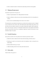
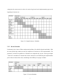
Semester one was primarily spent on doing background research into various aspects of the problem
and the proposed solution, and also the planning of the project. The gaps prior to week 4 were spent
preparing for the project and deciding which project to pursue. The gap in week 9 was unavoidable due
to a very heavy coursework load from other modules.
Figure 2.1: Original Semester 1 Schedule
Much more time was available in semester two, due to doing only 30 credits of module work compared
to 50 credits in semester one, and therefore it was planned to do the bulk of the implementation and
evaluation in the second semester. It was planned to do some preparatory work, such as becoming familiar with the libraries to be used and parsing .LSA files for handling LiSA (a Library of Scheduling
Algorithms which may provide some calculations for the sub problem solving) interaction, in the inter-
6
vening time after semester one in order to be ready to begin work on the implementation proper at the
beginining of semester two.
Figure 2.2: Original Semester 2 Schedule
2.2.2
Revised Schedule
Unfortunatly, due to bouts of illness and personal problems, this schedule slipped considerably. With
the exam period being reached just after the completion of iteration one of the implementation. The
preparatory work that was planned over Christmas was completed only in parts, with no great depth
- much more consultation of manuals and reference materials was needed during the implementation
process than was desired due to this, contributing to the difficulty in staying to schedule.
Figure 2.3: Revised Schedule
7
Therefore a new plan was drawn up for the period after examinations. A break was included in order to
attempt to recover enough to be able to fully focus on the project work. Work commenced on Wednesday the 4th of July. The new deadline for completion was at first estimated as ‘before the end of August
2007’ and later confirmed to be Wednesday the 29th.
8
Chapter 3
Background Research
3.1 Scheduling Theory
3.1.1
Introduction to Scheduling
Scheduling is a branch of Operational Research that appeared in the 1950’s. Operational Research
is involved with the solving of optimisation problems mathematically. Scheduling can be defined as
“a decision-making process [. . . ] dealing with the allocation of scarce resources to tasks over time.”
(Pinedo, 2001). The resources can be anything from machinery in a factory to CPUs in a computer, they
are generally referred to in scheduling as ‘machines’. The activites, or ‘jobs’ likewise represent tasks
such as spray painting an automobile or the execution of a computer program. As such, scheduling has
become an important field relevant to a great variety of real-world applications.
3.1.2
Terminology
In scheduling, problems are described in a standard format, the α |β |γ notation, where α is the number
of machines, γ is the objective function, and β being any additional restrictions on the problem e.g.
release dates for jobs. For example, the problem 1|r j |Lmax would be the problem of minimising the
maximum lateness of a job, that is, the maximum value of each job’s completion time minus its due
9
date (including negative values) on a single machine where jobs have release dates. The problem I will
be considering will be J||Cmax , minimising the makespan, that is minimising the total time consumed
to process all jobs, of a Job Shop problem. This problem can be decomposed into sub-problems of the
1|r j |Lmax type. (Shakhlevich, 2006)
3.1.3
The Job Shop Machine Environment
In scheduling terminology, a Job Shop refers to a system where all jobs have a fixed route through an
arbitrary number of machines, and the routes can differ job by job. For example, consider a furniture
factory, with 2 machines. The factory produces tables and chairs. All chairs are first processed by
machine 1 and then by machine 2. Conversely, all tables are first processed by machine 2 and then
machine 1. The Job Shop problem is determining the most efficient manner in which to schedule all
jobs across the available machines to the objective function, so that they do not violate their machine
order constraint. This project will only be considering the makespan, Cmax , as the objective function.
3.1.4
Computational Complexity
Section 2.1 introduced the concept of NP-Hardness and its consequences to algorithm design. The time
complexity of an algorithm is of vital importance to its real-world application; if an algorithm will take
years or even centuries to compute a solution it has no value when a solution is needed within an hour
or a day. Computational Complexity theory builds a mathematically founded framework for explaining
why some problems are fundamentally more difficult to solve than others. (Shakhlevich, 2006)
In the field of Computer Science, the running time of algorithms is usually represented in the ‘Big-O’
notation. This is a measure of the maximum number of basic operations, such as elementary arithmetic
and comparisons, that an algorithm will evaluate before termination. The number of operations can be
calculated by inspecting the algorithm and calculating the number of operations as a function of the
size of the input. A simple example is that of a linear search algorithm - the algorithm examines each
item in turn looking for the search item, so has a maximum of n comparison operations to perform if
there are n items to examine. We say the algorithm has running time bounded by O(n). As we are
only concerned with how the algorithm performs for large inputs, only the dominating term is kept; an
algorithm with 2n2 + 4n + 1 operations will have running time O(n2 ). Problems which can be solved
by polynomially-bound algorithms belong to a class of algorithms called P. As discussed before, the
10
Job Shop problem belongs to the NP-hard class of problems. No efficient (poly-time) algorithms have
been found for any NP-Hard problems. Combined with the fact that an NP-Hard problem can be proved
to be as difficult as another NP-Hard problem, it is widely regarded that no efficient algorithm can be
found to solve any NP-Hard problem. This is why other techniques like heuristics are vitally important
in real-world applications in which NP-Hard problems occur. (Pinedo, 2001)
3.1.5
Disjunctive Graph Theory
The Job Shop problem can be formulated as a Disjunctive Programming problem and represented on
a disjunctive graph Roy and Sussman (1964). Disjunctive Programming is a form of Mathematical
Programming (i.e. Optimisation) in which disjunctive constraints are allowed. This sets aside Disjunctive Programming from the more well known Linear Programming which only allows conjunctive
constraints those constraints which must all be met for a solution to be feasible. A set of constraints can
be called Disjunctive if at least one [. . . ] has to be satisfied but not necessarily all (Pinedo, 2001). The
Job Shop problem can be formulated as such an optimisation; however, this does not imply that there is
a simple method to find the solution (Pinedo, 2001).
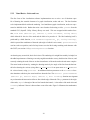
A disjunctive programming formulation of a Job Shop problem can be visualised in an understandable way with a disjunctive graph (Roy and Sussman, 1964). A disjunctive graph is a directed graph
G = (N, A, B), where N is the set of nodes, and A and B are sets of arcs, conjunctive and disjunctive respectively. The nodes of N correspond to the operations (i, j), that is job j = 1...n on machine
i = 1...m. The conjunctive (or solid) arcs represent the routes of the jobs. If there exists an arc such
that (i, j) → (k, j), then job j is processed on machine i and then on machine k. Conversely, the order
of jobs on a machine (i.e. operations that belong to two different jobs and that have to be processed on
the same machine (Pinedo, 2001)) is represented by a pair of disjunctive (or broken) arcs of B, which
travel in opposite directions. The arcs of B form m cliques (a subset in which all nodes have an arc
between them) - that is, one for each machine, all operations belonging to a clique are performed by the
same machine. The values of all arcs exiting a node are equal to the processing time required by that
operation. Two additional dummy nodes U, the source, and V , the sink, are added to the start and end of
the graph, and connected via conjunctive arcs to the first or last operation of each job respectively. Arcs
emanating from U have 0 length, and those entering V naturally have the length of the processing time
of the operation they are emanating from. (Pinedo, 2001)
11
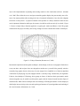
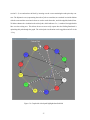
Figure 3.1: Disjunctive graph example
Figure 3.1 illustrates how conjunctive arcs (the black arrows) represent job order for each machine,
where each of the three conjunctive paths represent a single machine, therefore this particular graph
is of a 3 machine problem. The pairs of disjunctive arcs (the coloured arrows) form cliques which
represent the machine order for each job. A feasible schedule (i.e. one that can actually be performed
in practice) is an acyclic (i.e. all conjunctive and disjunctive arcs combined do not create any cycles)
disjunctive graph, where each pair has had one direction removed. For a discussion of why this is the
case, see Pinedo (2001).
3.1.6
The Shifting Bottleneck Heuristic
The Shifting Bottleneck heuristic was devised by Adams et al. (1988). It works by repeatedly solving
a single machine sub-problem using an algorithm devised by Carlier (1982). It is one of the most successful heuristics devised for the J||Cmax problem (Pinedo, 2001).
In the algorithm graph G is the full disjunctive graph we are working on. The set M0 is a subset of the
machines which have already been scheduled. The empty set (i.e. the set which has no elements) is
denoted by . Cmax (M0 ) denotes the makespan of the currently scheduled machines. There follows a
summary of the algorithm (Modified and corrected from the summary in Pinedo (2001)):
12
Step 1: Initialisation
Set M0 = G contains only the conjunctive arcs
Cmax (M0 ) = the longest path in G
Step 2: Analysis of machines yet to be scheduled
For each machine i in the set M − M0 :
Generate an instance of 1|r j |Lmax
(Where r of operation is equal to the length of the longest path in G from the source U to
node (i, j), and the due date of the operation equal to Cmax (M0 )(length of the longest
path from (i, j) to the sink V processing time of (i, j) ))
Minimise Lmax in each of these sub-problems
Let Lmax (i) denote the minimum Lmax in the sub-problem of machine i
Step 3: Bottleneck selection and sequencing
Let Lmax (k) =the largest Lmax (i) of the machines in M − M0
Sequence machine k by the sequence found in Step 2 for that machine
Insert the corresponding disjunctive arcs into G
Insert k into M0
Step 4: Resequencing of previously scheduled machines
For each machine i in M0 − k:
Remove the disjunctive arcs from G
Reformulate the 1|r j |Lmax sub-problem from the current G
Find the sequence that minimises Lmax (i) and insert the corresponding disjunctive arcs into
G
Step 5: Stopping Criterion
If M0 = M then STOP, else go to Step 2
13
Clearly this is a complex algorithm, with steps 2 and 4 being particularly confusing. Step 2 attempts
to schedule each machine as efficiently as possible according to the sub-problem. Step 4 reorganises
machines which are already scheduled by the current graph generated from this iteration. This can either
increase or decrease the optimality of the solution and there is significant scope for investigation on how
this step is best implemented.
3.2 Visualisation
3.2.1
Graph Layout Algorithms
The drawing of graphs for visualisations is an area into which considerable research has been conducted
(Chen, 1999). By only allowing for hard-coded problems in the visualisation it will be possible to avoid
the difficulties involved with drawing an arbitrary graph, as the structure of the hard-coded examples
will be known. However, while a small number of examples may be sufficient for teaching purposes,
it would greatly enhance the user base of the software if it could solve user inputted problems, which
would also allow for greater scope in teaching. This would require implementation of a graph drawing
algorithm suited to the disjunctive graph model. The layered layout algorithm described by Sugiyama
et al. (1981) would be one suitable choice. However, there are many algorithms to be considered should
the software be expanded in this manner. (Pajntar, n.d.; Chen, 1999). The problems these algorithms
are devised to tackle are themselves complex; the minimisation of edge crossings in a consecutive layer
of a Sugiyama graph has been proven to be NP-Hard. (Garey and Johnson, 1983)
The widely used C++ Boost Library (see section 3.1.2) has several useful classes available for the internal representations of graphs, and importantly several pre-implemented graph layout algorithms which
can utilise this internal representation. However, not all of the layout algorithms available are suitable
for the disjunctive graph model; the Kamada-Kawai Spring layout algorithm (Kamada and Kawai, 1989)
works by modelling a system of springs pulling vertices into place, where “The strength of a spring between two vertices is inversely proportional to the square of the shortest distance . . . between those two
vertices. Essentially, vertices that are closer in the graph-theoretic sense will have stronger springs and
will therefore be placed closer together.” (Lee et al., 2001) This approach would perhaps work well
for representing the job shop problem, with the vertices representing machine cliques closer together,
14
however the algorithm only works on connected, undirected graphs, and the disjunctive graph model is
directed (that is its arcs have a beginning and an end, and may only be traversed in one direction).
Figure 3.2: Layout created by Kamada-Kawai algorithm (NWB-Team, 2007)
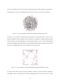
The library also provides the Fruchterman and Reingold (1991) algorithm which is another ‘forcedirected’ algorithm, follows an iterative process whereby the ‘temperature’ mitigates movement of the
vertices, and as it ‘cools’ the probability of vertex movement reduces. (Lee et al., 2001) This algorithm
works for unweighted, undirected graphs, and as stated already, the disjunctive graph model is directed
and is in fact weighted (the arcs have an associated cost for traversal) also.
Figure 3.3: Layout created by Fruchterman-Reingold algorithm (NWB-Team, 2007)
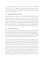
The Gürsoy-Atun (Gürsoy and Atun, 2000) algorithm is suitable for any directed graph, weighted or
unweighted. However, it differs from the previous algorithms in that it does not strive for a visually
15
pleasing result but rather to fit vertices into a predefined topography (figure 2.2), which means it is not
very suitable for clear display of data. This is also a problem with the ‘random’ layout provided by
Boost, where vertices are randomly spread between defined bounds.
Figure 3.4: Possible topologies for Gürsoy-Atun layout (Lee et al., 2001)
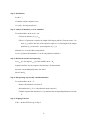
Finally, there is a simple circle layout algorithm, where vertices are arranged equally from one another
around a cricle with a defined radius. While not ideal this kind of layout will keep nodes separated and
easy to identify. The main concern with such a layout is that the overlapping of arcs would become a
bound on the size of the problem easily visualised in this manner.
Figure 3.5: Basic circle layout (NWB-Team, 2007)
3.2.2
Other Graph Visualisation Techniques
Even with an effective layout algorithm, large graphs can become too large to physically be displayed in
their entirety without special hardware such as a power wall. A traditional technique to overcome this
16
issue is the implementation of panning and zooming controls to the visualisation software. (Herman
et al., 2000) These allow the user to navigate around the graph to display the part currently most of interest. One major problem with zooming is the loss of contextual information - how does this subgraph
fit into the overall picture? A proposed solution to this problem is a fisheye distortion which focuses
on the important information and keeps the context viewable but with successively less detail. Figure
3.5 shows a simple fisheye distortion applied to a regular grid. (Sarkar and Brown, 1994) The graphs
considered in this project will likely not be large enough to need to consider these kinds of techniques.
Figure 3.6: Fisheye Distortion (Herman et al., 2000)
Incremental exploration and navigation techniques, which display to the user a subgraph of limited size
at any one time, and navigate from one subgraph to another are a powerful idea generally suited to
extremely large graphs, however there may be some margin for a simplified use of them in algorithm
visualisation by displaying only the subgraph which is currently being considered by the algorithm.
Likewise, the technique of Clustering, where groups or classes of data have their representative nodes
clustered together, may be useable on a disjunctive graph, with the clusters formed from the cliques of
machine nodes. Both of these techniques have the advantage of limiting the number of items displayed,
which helps increase clarity to the user and speed up performance of layout algorithms and rendering of
the visual elements. (Kimelman et al., 1994)
17
3.2.3
Additional Considerations
The use of colour is an important consideration for the visualisation as “Misinterpretations due to inappropriate choice of color sequences, poor use of [. . . ] differing color characteristics [. . . ] are evident
in many visual presentations of data” (Hutchins and Robertson, 1994). However an effective use of
colour can help convey information to the user - the primary purpose of a visualisation. Animation is
another useful tool, especially for representing changes in data over time or the progress of an algorithm.
(Thalmann, 1990)
18
Chapter 4
Analysis & Design
4.1 Useful Software and Libraries
4.1.1
LiSA - Library of Scheduling Algorithms
LiSA is a library of scheduling algorithms comprised of three parts. The LiSA core, written in C++,
provides implementations of several useful data structures, for use internally and within external algorithms. The LiSA core software can determine a problem’s complexity via problem reduction and a
database, and automatically select an algorithm from the library to solve it. The GUI component of
LiSA is written in Tcl/Tk for cross-platform usability, and allows the user to input problems of many
different types and greatly varied attributes. The GUI displays the results of algorithms as Gannt charts
or a sequence graph, and allows users to edit the solution by manually manipulating the job order of the
solution. (LiSA-Team, 2003)
All of LiSA’s algorithm modules are implemented externally as stand-alone executables with two command line parameters. These parameters pass the input and output .LSA files to the module, which
are of a simple text format. These modules tend to be written in C++ which gives them access to the
large range of data structures in the LiSA core. (LiSA-Team, 2003) The LiSA implementation of the
19
Branch & Bound algorithm could be used to calculate exact results for the subproblems generated by
the Shifting Bottleneck procedure. Alternatively the Dispatching Rules (Dispatching Rules are efficient
algorithms which solve some simple scheduling problems exactly, but are also effective heuristics for
many more complex problems) implementation could be used to provide a computationally faster, but
possibly non-optimal solution. However, the Branch & Bound algorithm should be fast enough for the
small input sizes planned.
LiSA could be used as a testing environment for the algorithm implemented in the project, but more
importantly the visualisation software will have to parse the output files, and write correctly formatted
input files, if manual transferral of the subproblem solutions are to be avoided. LiSA does come with an
implementation of the Shifting Bottleneck procedure, which can be used to evaulate the performance of
this project’s implementation.
4.1.2
Boost Graph Library
Boost is a collection of “free peer-reviewed portable C++ source libraries”, designed to work well with
the C++ Standard Template Library(Boost-Team, 2007). The Boost Graph Library (BGL) is a library of
classes for representing graphs of many different types and structures. This generic interface will make
implementing a disjunctive graph type easier than creating such a data-structure anew. The BGL also
provides many graph related algorithms:
• Shortest Path Algorithms
Including:
– Dijkstra
– Bellman-Ford
– DAG
– Johnson All Pairs
– Floyd-Warshall All Pairs
• Minimum Spanning Tree Algorithms
• Connected Components Algorithms
• Maximum Flow and Matching Algorithms
20
• Sparse Matrix Ordering Algorithms
The inclusion of shortest path algorithms is important as they may be adaptable to longest-path algorithms, needed for calculating due dates of jobs in the 1|r j |Lmax subproblem, and the critical path which
represents the solution to the J||Cmax problem. In fact, the DAG (Directed Acyclic Graph) shortest path
algorithm is trivially modified to give a longest path algorithm, as it works for negative edge weights.
Simply invert the sign of all weights in the graph, making the longest path(s) into the shortest. It is
very helpful that the disjunctive graph model is a DAG; the longest-path problem is NP-Hard for most
graphs, and the DAG problem is “about the only interesting case of longest path for which efficient
algorithms exist”. (Skiena, 1997)
4.1.3
OpenGL
OpenGL (Open Graphics Library) is a cross-platform, cross-language graphics programming API which
has become an industry standard. The author has two years experience in writing OpenGL software
using C++. OpenGL itself does not offer any support for windowing systems or I/O control. The
programmer must either use platform-specific window and I/O APIs or third party toolkits designed for
making simple, cross-platform OpenGL applications.
4.1.4
GLUT and Alternatives
GLUT (OpenGL Utility Library) is one such library. Only a few lines of GLUT code are required to
create a window which can render OpenGL content:
int main(int argc, char **argv)
{
glutInit(&argc,argv);
glutInitDisplayMode(GLUT_RGB);
glutInitWindowSize(100, 100);
glutCreateWindow("TEST");
glutDisplayFunc(display);
glutMainLoop();
21
return 0;
}
These six lines of code will initialise a new window with the title ‘TEST’, of size 100 by 100 pixels, with a RGB colour buffer. The glutDisplayFunc(display); call sets up a call-back to a
function called ‘display’ which will do the actual rendering. The glutMainLoop(); call initialises
the program into a loop which checks each call-back function that has been registered. A considerable
limitation of the original GLUT library is that this function never returns, making it impossible for the
programmer to switch control to and from GLUT, also causing the program to terminate when the window is closed. The original GLUT library is no longer maintained, the last update being released in
August 1998. (FreeGlut-Team, 2005)
FreeGlut is a “completely OpenSourced alternative to the OpenGL Utility Toolkit (GLUT) library”
(FreeGlut-Team, 2005), developed to continue development of the GLUT codebase and overcome some
licensing issues with the original GLUT. FreeGlut adds a glutLeaveMainLoop(); function which
allows the programmer to explicitly exit the glutMainLoop(), restoring control to the function
which called it. (FreeGlut-Team, 2005).
Another GLUT alternative, itself an offshoot of FreeGlut, is OpenGLUT, which takes the bug fixes of
FreeGlut and aims to add further functionality on top of the original GLUT feature set. As such, it also
supports the glutLeaveMainLoop(); function.(OpenGLUT-Team, 2005)
4.1.5
GLUI and Alternatives
There are a wide variety of Graphical User Interface (GUI) libraries available which are cross-platform
and cross-language, such as GTK, fltk and wxWidgets. As a GUI driven interface is not a prime concern
for this project and with development time limited, it would not be ideal to have to learn to use another
independant library to implement it. Therefore a pure OpenGL/GLUT based GUI library is desirable
should a GUI be implemented.
Several such libraries exist, but the most powerful and up to date one is probably the GLUI library, with
the latest version released in July of 2006 (Stewart, 2006). GLUI has all the required functionality for
22
a simple GUI for the project software with the important ability to directly render OpenGL code within
its windowing system.
4.2 Language and Platform Choice & Justification
The project should be cross-platform for several reasons. Being cross-platform will allow it to be developed on both linux and windows machines used within the School of Computing and on the author’s
personal computer. It will also allow the final software to be built on either platform for the demonstration and teaching purposes for which it is intended, likewise it will increase the number of students able
to experiment with the software on their own hardware.
As was discussed in section 2.2, the project will follow an Object-Oriented (OO) design philosophy,
as such, the chosen language must support the OO paradigm. The author has experience with three
such languages: Python, Java and C++. The author only has OpenGL experience with C++, however
the API is available on all three languages, with relatively minor differences in naming convention and
programming style. Python syntax is particularly simple which would tend to increase the pace of development, however, the author feels that in some cases the syntax can become a hindrance when trying
to implement particularly complex pieces of code which may be simpler in a more powerful language.
Therefore Python can be ruled out as a language choice.
The author has most experience with Java, and has experience with building GUI driven programs with
the standard Java Swing API, whereas a GUI in a C++ implementation will have to use another library
such as GLUI (see section 4.1.5). However a GUI is not a priority, the LiSA core and algorithms are
written in C++, and the C++ Boost library has several classes which are necessary for the implementation of the Shifting Bottleneck algorithm (see section 4.1.2). Therefore C++ is the language which
has been chosen. As further justification, the Boost library is very well documented and stable, whereas
Java alternatives, whilst available, are not as well documented and are missing some of the functionality
present in Boost. C++ continues to be highly used in the computing industry and completing a large
project in it will be a beneficial learning experience.
23
4.3 Flow of Control
There follows a diagram illustrating the flow of control within and between the scheduling and visualisation parts of the software.
Figure 4.1: Flow of control
24
4.4 UML: Concept-level Class Diagram
There follows a UML-style Concept-level class diagram which illustrates the classes which make up the
software and how they relate to one another. This was used as a design guide when implementing the
system.
Figure 4.2: Concept-level Class Diagram
25
Chapter 5
Implementation
5.1 Iteration 1
5.1.1
Goals of Iteration 1
Iteration 1 of the implementation focused on the scheduling aspect of the software. The goals were to:
• Create the internal representation of the disjunctive graph
• Adapt the Boost Graph Library DAG Shortest Path algorithm to a longest path algorithm which
will accept the disjunctive graph as input
• Write code to transfer subproblem solutions from LiSA
• Combine the modules to implement the Shifting Bottleneck procedure
5.1.2
Subproblem and LiSA Branch & Bound
It was decided to attempt an automatic method of data transfer from the start, rather than waste time
implementing a clumsy manual interface that would require the user to have a full install of LiSA
and input both the parameters into LiSA and then import the results back into the software. As LiSA
algorithms are all implemented as separate executables, only the Branch & Bound executable itself
26
needs to be packaged with the software. The input and output files, in a LiSA specific format, are
passed to the algorithm executable via the commandline. A simple class, ExternalAlgorithm was
written to run the executable via a system call:
std::string command = "bin\\" + name + " " + input + " " + output;
system(command.c_str());
This small bit of code was all that was required to call the algorithm, input and output are attributes
of the class which are passed to the constructor. They are merely strings containing the filename of the
input and output .LSA files.
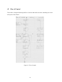
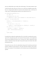
Writing a class to read and write the LSA files themselves was a more complex task. When run externally to LiSA the Branch & Bound executable outputs only the job order (see Appendix B), so the class
has to reconstruct the completion dates of each job on the machine, compute the lateness for each job,
and then pick the largest lateness value, Lmax . An example output.lsa follows:
<SCHEDULE>
m= 1
n= 3
LR= {
{
3 }
{
2 }
{
1 }
}
</SCHEDULE>
The lines m and n correspond to the number of machines and jobs in the problem respectively. The
LR section indicates job orders - in this example, the job order is 3,2,1. The SubProblem class encapsulates the idea of the subproblem and provides the functionality to handle LSA files. First, bool
SubProblem::readLsa() is called, which uses a simple while-loop checking for the end-of-file
to read the input.lsa into a single string, returning false if this operation is unsuccessful and the result
of the function call to bool SubProblem::parseLsa(std::string filestring) otherwise. This function jumps to the LR section of the input file held in the string, at which point it begins
to iterate character by character until it finds a number, which it then adds to a map (a kind of key-value
27
pair array) which holds the data on which job has which ordering. This iteration terminates when it
reaches the end of the string. This piece of code is not a very efficient way to handle the parsing of files,
however it is simple and short and the files concerned are short and simple in nature, so efficiency is not
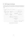
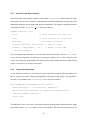
a major concern. The following function can then be used to obtain the value of Lmax :
int SubProblem::getObjective() {
int lmax = 0;
std::map<int,int> CD, LIJ;
// completion of first job is minimum of 0 and release date of
that job + its processing time
CD[LR[1]] = std::max(0,RD[LR[1]]) + PT[LR[1]];
if (n > 1)
for (int i=2; i < n+1; i++)
CD[LR[i]] = std::max(CD[LR[i-1]], RD[LR[i]]) + PT[LR[i]];
for (int i=1; i < n + 1; i++) {
LIJ[LR[i]] = CD[LR[i]] - DD[LR[i]];
lmax = std::max(lmax,LIJ[LR[i]]);
}
return lmax;
}
Essentially this first calculates the completion date (CD) of a job, which is its start date plus its processing time (PT), starting dates being either 0, the release date of the job in question, or the completion date
of the previously scheduled job if that job is late. The lateness (LIJ), which is completion date minus
due date, is calculated for each job and a simple for-loop picks the largest value of lateness found, which
the function then returns.
The input file writer creates a file with a standard header setting up the LiSA problem type and control
parameters, and adds in the processing times, release dates and due dates which have been passed to
the class in its constructor. The values themselves will be calculated as part of the Shifting Bottleneck
algorithm.
28
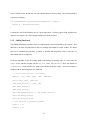
5.1.3
Internal Graph Representation
The internal graph representation is held in a class named GraphHandler which contains the graph
data structure itself as one of its attributes, and implements methods for adding and removing edges, and
additionally methods to call the longest path and layout algorithms. The disjunctive graph data structure
is built upon the BGL’s adjacency list data type as follows:
typedef adjacency_list <
listS,
// Store out-edges in a std::list
vecS,
// Store vertices in a std::vector
directedS,
// The graph is directed
property<operation, std::string>, // name of a node
property < edge_weight_t, int >
// weight of each edge
> DisjunctiveGraph;{
There are additonal type defintions to set up the vertex and edge descriptors, and the PositionMap
used by the layout algorithm. An adjacency list represents a graph by way of a list of edges for each
vertex. As the disjunctive graph model is directional, the lists can be further limited to just edges leaving
vertices, as this will cover all edges in the graph.
5.1.4
Longest Path Algorithm
As was detailed in section 4.1.2, the Directed Acyclic Graph shortest-path algorithm provided by the
BGL is trivially converted to a longest path algorithm by negating all edge weights. The algorithm is
accessed via two methods of the GraphHandler class. The first of which is:
bool GraphHandler::doLongestPath(int source) {
vertex_descriptor s = vertex(source, disGraph);
dag_shortest_paths(disGraph, s, predecessor_map(&parents[0])
.distance_map(&distances[0]));
return true;
}
This initialises a vertex as the source of the longest (shortest) path algorithm, and then passes the graph
representation object disGraph and the source to the algorithm. The other function parameter is the
29
array in which to store the parents of a node and the distances between them. The second method is
even more elementary:
int GraphHandler::getLongestPathLength(int target) {
return 0 - distances[target];
}
It returns the value in the distances array to a given target node. As all the edge weights, and therefore
distances, are negative, the value is negated again before being returned.
5.1.5
Shifting Bottleneck
The Shifting Bottleneck procedure itself was implemented as the main method of the software. This
illustrates a less than strict adherance to the OO paradigm and should have been avoided. The initial
plan was to implement the procedure as quickly as possible and encapsulate it into a class later on,
unfortunatly this never happened.
Firstly the algorithm creates the internal graph representation by pushing pairs of vertices onto the
edges vector, and their weights onto the weights vector. The gHandler object (an instance of
GraphHandler) then initialises the graph representation with those edges. Next each machine’s
attributes and job processing times are initialised:
// initialise machine 1 attributes
map<int, int> inPT, inRD, inDD, jobOrder;
vector<int> jobs, vertices;
jobs.push_back(1); // set jobs
jobs.push_back(2);
jobs.push_back(3);
vertices.push_back(2); // set graph vertices
vertices.push_back(5);
vertices.push_back(10);
// set machine 1 processing times
inPT[1] = 5;
inPT[2] = 5;
30
inPT[3] = 5;
This is repeated for each machine in the problem. Now the longest path from the artificial source node
U of the graph to the sink V is generated to calculate the initial value of the objective function, the
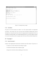
makespan, Cmax . This is then outputted to the user who is prompted to continue onto step 2 (see section
3.1.6) of the Shifting Bottleneck procedure.
Figure 5.1: Screencap of step 1 output
Step 2 of the algorithm generates a 1|r j |Lmax subproblem based on each machine using the longest path
algorithm to calculate the release and due dates of jobs. The results are outputted and the user is once
again prompted to continue.
31
Figure 5.2: Screencap of step 2 output
In step 3 the so called ‘bottleneck’ machine is then selected. Unfortunatly, due to a bug in the LiSA
Branch & Bound module, the values of Lmax were incorrect in some instances. This forced the unpleasant situation of hardcoding Lmax results in these cases. This also lead to the hardcoding of bottleneck
selection, though with more time this could have been implemented using a relatively straightforward
loop to select the machine with the largest Lmax . The selected disjunctive arcs (see section 3.1.5) are
then added into the graph using the bool GraphHandler::addEdge(IntPair edge, int
edgeWeight) method. Cmax is then recalculated in the same manner as before and the bottleneck machine added to the vector representing M0 , the set of scheduled machines. The information is outputted
and the user prompted to continue. (see figure 5.3)
Step 4 performs a check on the number of machines in M0 , if it is one then there is no resequencing
required. Resequencing itself was felt a complex and unnecessary step of the algorithm to implement,
and so was disregarded. This may reduce the quality of the final solution, but as with any heuristic
there is a trade off between processing time and solution quality. Step 5 performs a second check on the
number of machines in M0 , if it is equal to the number of machines in M, i.e. all machines have been
scheduled, then the algorithm terminates. Otherwise, the algorithm continues again from step 2.
32
Figure 5.3: Screencap of step 3 output
5.1.6
Conclusions
The goals set out for this iteration were achieved. All of the required modules were implemented
successfully. On the negative side, due to the bug in the LiSA Branch & Bound module, and the
unfortunate loss of large amounts of time to illness, the implementation of the algorithm itself was not
as polished as would be desirable. In several places hardcoded ‘hacks’ were used as temporary measures
to overcome some problems, and never properly replaced with more efficient and better designed code.
5.2 Iteration 2
5.2.1
Goals of Iteration 2
Iteration 2 of the implementation focused on the visualisation aspect of the software. The goals were to:
• Construct a set of basic functions for the rendering of a graph
• Utilise the basic functions to draw a disjunctive graph
• Integrate the visualisation with the scheduling part of the software
33
5.2.2
Visual Basics - Nodes and Arcs
The first focus of the visualisation software implementation was to write a set of functions capable of drawing the essential elements of a graph visualisation; nodes and arcs. The first function
to be implemented dealt with node rendering. In a hand-drawn graph visualisation, nodes are represented as labelled circles. Rather than write a new function for drawing a cirlce, gluDisk from the
standard GLU (OpenGL Utility Library) library was used. This was wrapped within another function, void node (GLfloat* p1, GLfloat r, GLint thickness, string label)
which allowed for the size of the node and the label to be passed to it. The label rendering itself is
performed by a third function, void renderString(GLfloat* p1, string inString),
which is passed the coordinates of the node (the origin of which is at its center). glRasterPos2f is
used to set the text position, and a for-loop iterates over the label string rendering each character with
the GLUT (see section 4.1.4) glutBitmapCharacter function.
Arc drawing may seem trivial, but in fact it is not. The rendering of a straight line certainly is simple, but
the added requirements of drawing a correctly-angled arrowhead to convey the direction of the arc, and
correctly orienting the ends of the arc on the circumference of the nodes makes the task more complex.
The arrow heads are drawn by rotating the drawing matrix by the angle of the line from the horizontal before drawing the vertices (using either GL LINE STRIP for an open arrow or GL TRIANGLES
for a closed arrow) using glRotatef. An additional boolean parameter to the ArrowHead function determines which way the arrow head faces down the line. The GLfloat* getPointOnNode
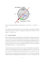
(GLfloat* p1, GLfloat angle, GLfloat r, bool incoming) function uses trigonometry to determine the intersection of the arc line with the edge of the node. The p1 parameter is the origin
of the node, angle is the angle of the arc line from the horizontal, r is the radius of the node circle and
incoming indicates if the arc is directed into or out of the node. Figure 5.4 illustrates the mathematics
used.
34
Figure 5.4: Trigonomtry determining arc-node intersection, a is angle. P1[0] = r ∗ sin(a), P1[1] = r ∗
cos(a)
The combination of these functions enables the arc to be correctly drawn, with its direction determined
by the ordering of the nodes it connects i.e. passing node A first then node B will draw an arc in the
direction A → B, and vice versa.
5.2.3
Graph Visualisation
With the fundamental drawing code implemented, the main challenge for drawing the graph itself becomes to correctly orient the nodes and determine between which nodes arcs should be rendered, and
of what type. The node positions are generated by the layout algorithm in the scheduling software, the
basic circle layout was chosen (see section 3.2.1). As the layout algorithm only interacts with nodes, and
the number of nodes remains static, the layout algorithm itself need only be called once, immediately
after initialisation of the gHandler object (see section 5.1.3).
During development the graph visualisation code was setup to draw a hardcoded example graph from
several arrays. When integrating the code into the scheduling software these arrays were reused with
the new data from the scheduling example rather than being replaced with, or copied from, the vectors
and maps utilised to store node information in the scheduling software. As with similar issues regarding
the implementation of the Shifting Bottleneck algorithm itself (see section 5.1.5), this approach can be
35
considered to be a poor, but expedient, compromise. Contrarily, arc rendering was improved by using
vectors controlled by the scheduling software, considerably reducing the length of code required and
enabling the arcs being rendered to be updated - visualising the progress of the Shifting Bottleneck algorithm through changes to the disjunctive graph.
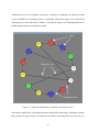
Figure 5.5: Graph with labelled nodes, conjunctive and disjunctive arcs
The nodes are rendered first, with a hardcoded colour determined by the machine on which the operation
they represent is being processed. The conjunctive arcs (those representing the routes of the jobs, see
36
section 3.1.5) are rendered next in black, by iterating over the vector containing the node pairs they connect. The disjunctive arcs (representing the order of jobs on a machine) are rendered in a similar fashion
with the same machine-associated colours as used to render the nodes, and with stippled (dashed) lines.
To further enhance the visualisation the critical path, which indicates Cmax , is rendered in stippled white
lines over the existing arcs. This allows the user to more easily capture how the Shifting Bottleneck is
optimising this path through the graph. The critical path visualisation can be toggled on and off via the
‘s’ key.
Figure 5.6: Graph with critical path highlighted and labelled
37
5.2.4
Conclusions
The goals set out for this iteration were achieved. The required modules were implemented, though
once again code clarity, and thus maintainability, were traded for expediency. The visualisation modules
were not encapsulated in a class as they should have been in order to follow the OO paradigm. This was
partially due to the author’s inexperience with graphics programming within an OO architecture, with
the basic architecture of the code coming from earlier work in taught graphics modules. On the other
hand, it also illustrates the point that the C++ language is not as strict at upholding the OO paradigm
as more modern languages such as Java, in which all code must be encapsulated as a class. Whether
or not this is a positive fact is an open topic for debate. Overall, the two major parts of the software
were completed, and integrated, using the proposed methodology, with some minor deviations due to
unforseen problems or for expediency.
38
Chapter 6
Evaluation
6.1 Evaluation Criteria
The evaluation criteria for this project are
• Extensibility - How easy will it be to extend the software to include new features?
• Quality of the algorithm solution - How close to the optimal is the computed value of Cmax ?
• Effectiveness vs. existing methods for teaching - Does the software have significant advantages
over other means of learning about the Shifting Bottleneck algorithm?
These three criteria are meant to offer an accurate, overall evaluation of the success of the project in
creating a useful learning tool.
6.1.1
Extensibility
Extensibility considers how easy it will be to add new functionality to the software and adapt current
functionality to new scenarios. First and foremost is the extention to an arbitrary, user-inputted Job
Shop problem, or the ability to load problems from some configuration file. This would require some
‘cleaning up’ of the current algorithm code. The code would be abstracted into a class, with currently
39
hardcoded functionality like bottleneck selection implemented as a method of the class. This refinement
in itself will be time-consuming, but likely not overly complex a task for an accomplished C++ (Or
indeed any other language focused on the Object Oriented paradigm) programmer.
Once this refinement has been implemented, it will become much easier to extend the software in other
ways, particularly the handling of arbitrary instances. An additional class to take the user input could be
written which passes the attributes of the instance of the Job Shop problem to the Shifting Bottleneck
class. Likewise this class could read from or write to configuration files which describe the Job Shop
instance and the calculated solution for further study, or perhaps as a pre-selected example for demonstrating as part of a lecture or coursework.
Another possible extention would be to implement the rescheduling step of the Shifting Bottleneck algorithm (see section 3.1.6). The framework for computing this step is already in the code, i.e. the checks
for when it should be performed, it just requires the actual logic of the step itself to be implemented again this could be a new method of a Shifting Bottleneck class. The software can easily be modified
to use the LiSA Dispatching Rules module instead of Branch & Bound, by changing the string which
looks for bb.exe and updating the configuration string written to input.lsa (see section 5.1.2).
6.1.2
Quality Of Algorithm Solution
The value of Cmax calculated by this implementation of the algorithm for the example instance is 25.
The LiSA implementation of the Shifting Bottleneck algorithm running on the fast setting also arrives
at a Cmax value of 25. In fact, this is the optimal value for this instance of the Job Shop problem, as confirmed by LiSA’s Branch & Bound examination. This is a very good result, especially as the additional
optimisation step of rescheduling is skipped in the implementation.
However, the instance used in the software is relatively simple, so that it is easier to understand and
visualise. It is reasonable to assume that for larger, more complex instances the lack of the rescheduling
step may negatively impact performance. As the software is meant primarily as a learning aid, and
not specifically as a tool for solving scheduling problems, the optimality of the solution is not of vital
importance – as long as the solution is not extremely wide of the mark.
40
6.1.3
Effectiveness vs. Existing Solutions
This section will attempt to evaluate how effective the software is compared to similar visualisation
tools and other methods of learning about the Job Shop problem and the Shifting Bottleneck algorithm.
RIOT/GRAAL - The Remote Interactive Optimization Testbed is “a new offering for the WWW audience providing interactive educational and research tools for optimization problems.” (Adler et al.,
2007). Of particular interest is the GRaph Applications AppLet (Goldschmidt and Hochbaum,
1998), a Java-written applet which contains visualisations for the Minimum Spanning Tree (MST)
and Travelling Sales Person (TSP) graph problems. It allows the user to draw their own graph
by placing nodes and arcs or can generate random instances of large sizes (upto 300 nodes) and
different arc densities. Several algorithms are implemented for solving the TSP problem, each visualisation moves step by step through the algorithm updating the graph and the speed of progress
is set by the user via a slider.
Figure 6.1: GRAAL visualisation of TSP
41
Overall, GRAAL is an impressive tool, and the user control over the visualisation and continual
updating of the graph (as opposed to the very discrete method implemented in the project, where
the graph is only displayed after each algorithm step has finished) are superior. However, GRAAL
does not consider any scheduling problems at all, and as such is not useful as a learning tool for
the problems with which this project is most involved.
LEKIN - LEKIN is “a scheduling system [. . . ] created as an educational tool with the main purpose of
introducing the students to scheduling theory and its applications.” LEKIN-Team (2002). LEKIN
features multiple scheduling environments, including the Job Shop, for which several variations
of the Shifting Bottleneck algorithm are implemented, and the ability to optimise for objective
functions other than Cmax . It comes with a set of more than 60 standard benchmark problems,
and also allows user input of problems and control over solutions by manipulating Gannt charts
with a drag and drop interface. LEKIN is developed to be used with the book by Pinedo (Pinedo,
2001).
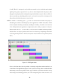
Figure 6.2: LEKIN gannt charts
However, the Gannt chart is the only method of visualising an algorithms solution and there is no
visualisation of the algorithm in progress. In this respect it is missing what is considered critical
functionality in the software produced in this project. LEKIN is a powerful tool both for solving
and learning about scheduling problems, but its all-encompassing nature means that there is less
42
focus on the particular problem (J||Cmax ) and solution which this project is about.
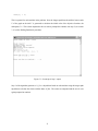
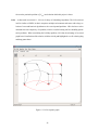
LiSA - As discussed in section 4.1.1, LiSA is a Library of Scheduling Algorithms. The LiSA software
itself is similar to LEKIN, in that it comprises multiple environments and comes with a large selection of exact and heuristic algorithms to solve user-inputted problems. LiSA also has a tool to
determine the time complexity of a problem, which is a useful learning aid for scheduling optimisation problems. When considering the Job Shop problem, LiSA has the advantage of an actual
graph-based visualisation of the solution, with the critical path highlighted, as well as having drag
and drop gannt charts.
Figure 6.3: LiSA sequence graph
43
However, the visualisation is again simply the final output of the algorithm. There is a second
visualisation comprised of a simple histogram which maps the progress of the value of the objective function, but this does not illustrate how the algorithm works - the key aim of this project’s
visualisation.
Book learning - Books are an important learning tool in any subject. Scheduling: Theory, Algorithms
and Systems (Pinedo, 2001), was the main information source for the author when learning about
the Shifting Bottleneck algorithm. The book was also referenced in many of the OR32 slides and
lectures in which the author gained a fundamental understanding of scheduling and the Job Shop
problem. Pinedo has a detailed explanation of the Shifting Bottleneck algorithm (upon which the
guide in section 3.1.6 is based, in modified form), and a walkthrough of an example, with several
illustrations of the corresponding disjunctive graphs. However, a book is only a one way learning
device - the lack of user interaction means that additional aids such as visualisation tools are still
very much of use.
Overall, the software produced by this project fills a niche for a Shifting Bottleneck oriented visualisation, which illustrates both the solution and the working of the algorithm. Better tools exist for
visualisation, but are missing the Shifting Bottleneck; likewise better implementation of the Shifting
Bottleneck are available, but struggle to fulfil the need for visualisation.
6.2 Evaluation vs. Minimum Requirements
The minimum requirements have been met, they are reproduced below with justifications of why and
how they have been met:
• Produce an implementation of the ‘Shifting Bottleneck Procedure’ - Iteration 1 produced a working implementation of the Shifting Bottleneck algorithm (see section 5.1.5) The exclusion of the
rescheduling step should not be seen as a failure to meet this requirement, as its exclusion was
planned, and has not been greatly detrimental to the quality of the solution outputted by the algorithm (see section 7.1.2).
• Produce visualisation software that may allow data interchange with LiSA for intermediate calculations - Iteration 2 produced a working visualisation software which was integrated with the
algorithm implementation, with no need for manual data interchange with LiSA.
44
• Write a brief user manual detailing the basic features of the software. - The brief user manual
covering installation and use of the software was completed, see appendix C.
Only one of the proposed extentions to the minimum requirements was acheived:
• Stand-alone software without the need for manual data interchange with other software - This
extention was fully implemented in Iteration 1, by the modules described in section 5.1.2.
• Permitting user-control over the decisions made by the algorithm in order to deepen the users
understanding - This extension was not implemented due to the failure to allow user-inputted
problems - the sample problem was not complex enough for user decisions to have a great impact
on the outcome.
• Problems defined entirely by user input - This extention was not implemented due to time constraints and the bug in the LiSA Branch & Bound module (see sections 5.1.5 and 5.1.6).
• Additional teaching materials such as lecture plans and coursework - This extention was not
implemented due to time constraints and the limited utility of the software without its extentions.
6.3 Conclusions
This project set out to produce an implementation of the Shifting Bottleneck heuristic and a visualisation
accompaniment which not only demonstrated the output but also the working of the algorithm. Overall,
this objective has been met, as have the minimum requirements for the produced solution. The implementations may not have been as exacting and methodologically pure as intended, nor the final software
as grandiose in its feature set as may be desired, but the project does fulfil its objective, and fills a niche
in the toolset for learning about the Job Shop scheduling problem and the Shifting Bottleneck heuristic.
As such, it can be considered a success.
45
Chapter 7
Further Development
7.1 Plan of Ideal Software
Further development on the basis of the current solution can produce a solution which meets the ‘ideal’
feature set that may be desired. Firstly, the issues encountered in development must be overcome with
the encapsulation of the Shifting Bottleneck into a class (see sections 5.1.5 and 7.1.1). This would allow
for the important extention of problems defined entirely by user input, and read/writing to configuration
files. (see section 7.2). With these changes, the software could be extended to allow user control over
the algorithms decisions (see section 7.2), which opens up a new level of interactive depth to the user.
In the ideal software, the visualisation would be displayed constantly, as part of a graphical user interface, and updated continuously by the algorithm, as in GRAAL (see section 7.1.3). User control over the
speed at which the algorithm and visualisation run would also be incorporated. Other elements of the
GUI would allow the user to track the progress of the value of Cmax and show Gannt charts illustrating
the schedule for each machine, as in LiSA (see section 7.1.3).
46
7.2 Other Possible Extensions
There are many other ways in which this work can be extended, a few examples are listed:
• Implement the algorithm for objective functions other than Cmax .
• Implement other means of solving the problem, such as Dispatching Rules and Branch & Bound
algorithms - this allows for research to be conducted into the trade off between speed and solution
optimality.
• Implement the rescheduling step - This could be done in a number of ways, allowing research into
the most optimal method of rescheduling the machines.
• Broaden the software to visualise other kinds of scheduling problems and corresponding algorithms.
47
Bibliography
J. Adams, E. Balas, and D. Zawack. The shifting bottleneck procedure for job shop scheduling. Management Science, 21:391–401, 1988.
I. Adler, K. Goldberg, and D.S. Hochbaum.
Riot – remote interactive optimization testbed.
http://riot.ieor.berkeley.edu/riot/ [27th August 2007], 2007.
Boost-Team. Boost c++ libraries. http://boost.org [27th August 2007], 2007.
J. Carlier. The one-machine sequencing problem. European Journal of Operational Research, 11:
42–47, 1982.
C. Chen. Information Visualisation and Virtual Environments. Springer-Verlag, 1999.
FreeGlut-Team. The freeglut project. http://freeglut.sourceforge.net [27th August 2007], 2005.
T. Fruchterman and E. Reingold. Graph drawing by force-directed placement. Software–Practice &
Experience, 21(11):1129–1164, 1991.
M.R. Garey and D.S. Johnson. Crossing number is npcomplete. SIAM J. Algebraic and Discrete Methods, 4(3):312–316, 1983.
O.
Goldschmidt
and
D.S.
Hochbaum.
Graph
algorithms
applet.
http://riot.ieor.berkeley.edu/riot/Applications/graal/graal.html [27th August 2007], 1998.
A. Gürsoy and M. Atun. Neighborhood preserving load balancing: A self-organizing approach. EuroPar Parallel Processing, LNCS 1900:324–341, 2000.
I. Herman, S. Marshall, and Melançon G. Graph visualization and navigation in information visualization: A survey. IEEE Transactions On Visualization And Computer Graphics, 6(1), 2000.
48
M. Hutchins and P. Robertson. An Approach to Intelligent Design of Color Visualizations. IEEE Computer Society, 1994.
T. Kamada and S. Kawai. An algorithm for drawing general undirected graphs. Information Processing
Letters, 31:7–15, 1989.
D. Kimelman, B. Leban, T. Roth, and D. Zernik. Reduction of visual complexity in dynamic graphs. In
Proc. Symp. Graph Drawing GD ’93, 1994.
L-Q. Lee, A. Lumsdaine, and J. Siek. The Boost Graph Library, 2001.
LEKIN-Team. Lekin – scheduling system. http://www.stern.nyu.edu/om/software/lekin/ [27th August
2007], 2002.
LiSA-Team. A library of scheduling algorithms. http://lisa.math.uni-magdeburg.de [14th December
2006], 2003.
NWB-Team. Network workbench. https://nwb.slis.indiana.edu/community/ [27th August 2007], 2007.
OpenGLUT-Team. The freeglut project. http://openglut.sourceforge.net [27th August 2007], 2005.
B Pajntar. Overview of algorithms for graph drawing. http://kt.ijs.si/Dunja/SiKDD2006/Papers/Pajntar.pdf
[14th December 2006], n.d.
M. Pinedo. Scheduling: Theory, Algorithms, and Systems. Prentice Hall, 2001.
B. Roy and B. Sussman. Les problemes dordonnancement avec constraints disjonctives. SEMA, Note
DS No.9 bis, 1964.
M. Sarkar and M.H. Brown. Graphical fisheye views. Comm. ACM, 37(12):73–84, 1994.
N. Shakhlevich. Or32 scheduling: Models and algorithms notes, 2006.
S Skiena. The Algorithm Design Manual. Springer-Verlag, 1997.
N. Stewart. Glui user interface library. http://glui.sourceforge.net [27th August 2007], 2006.
K. Sugiyama, S. Tagawa, and M. Toda. Methods for visual understanding of hierarchical system structures. SMC, 11(2):109125, 1981.
N. Thalmann. Scientific visualization and graphics simulation. John Wiley & Sons, Inc., 1990.
49
Appendix A
Personal Reflections
I began this project with little knowledge of scheduling itself, nevermind the more advanced topics of the
Job Shop problem and the Shifting Bottleneck heuristic. Fortunatly the OR32 module was in semester
1, and helped me to rapidly understand the concepts I was dealing with. That module however did not
cover the Shifting Bottleneck heuristic, and a lot of time had to be spent reading, understanding, and
trying out the algorithm for myself.
The decision to implement everything in C++ was in part forced by the availability of functionality that
was required in C++ libraries. Transferring the Object Oriented skills learnt in Java to C++ was quite a
challenge, but an enjoyable one, and generally a positive learning experience.
I ran into many problems throughout the completion of this project. Technical, medical and personal
problems all hampered my progress. My advice to future students is to be as open as you can with your
supervisor and other members of staff who are there to help you. I often found that coming back to a
technical issue after distracting myself with some other work, and conversation with other students on
how they would approach the problem to be beneficial in the quest to find the inspiration for the elegant
solution to my problem.
50
Due to the more personal problems, I found both the software implementation and the report write up
challenging tasks. It was tremendously difficult to focus on getting the work done, but now that it finally
is I am satisfied with what I have produced. I took the decision to postpone my submission, and hence
my graduation, so that I could make up for some of the time lost. Whilst it is quite unsettling to not have
graduated with the friends I’ve found over the past three years, I feel it was the right decision to make,
that the work I have produced is all the better for it, and I realise that had I not taken this decision, I
would have been grossly disatisfied with the quality of the work I had done up to that point, as I felt it
did not reflect what I was capable of producing. Here again I would advise future students that compromises are necessary, both on the level of technical decisions, and for the unfortunate few, more difficult
decisions which may be faced.
Perhaps if I had found a project which better held my interest personal problems would not have intruded
so much. On the other hand, it may be a misconception that I wasn’t interested in this project, certainly
I was dubious at the beginning, but on reflection the learning experience and the challenge made it quite
enjoyable, despite the myriad of problems and stresses encountered.
51
Appendix B
Correspondence with LiSA Team
From:
Craig Lawrence
To:
[email protected]
Date:
28 February 2007 20:17
Subject: Input .lsa to bb module
Hello,
I’m attempting to use the bb external algorithm without LiSA, and I’m having some difficulties preparing a .lsa file to input into it.
The largest problem being that when run by LiSA there is a CIJ section in ¡SCHEDULE¿ whereas when
running the bb program standalone does not seem to generate this, and only gives the job order (LR)
without the completion times (CIJ) without which I cannot easily determine the obtained value of the
objective function and consequently, the output is of very limited use.
Is there a way to generate this information when running the program standalone, or does LiSA add this
information itself?
Regards,
C. Lawrence
52
From:
Heidemarie Braesel
To:
Craig Lawrence
Date:
01 March 2007 08:47
Subject: Re: Input .lsa to bb module
Hello,
for which problem do you want apply the branch and bound algorithm? Please, sent us your input file,
that we can reconstruct the mistake.
We are working hard on the next version of LiSA, then more algorithms are available, for instance
beam-search algorithms and genetic algorithms.
The file format changes to xml. The use of external algorithms will be simplified. It will be posible, to
start some hybrid algorithms: for instance: start with a set of dispatching rules, take the best and apply
an iterative heuristic.
The algorithms are implemented, but the help is under reconstruction.
Regards - H. Brasel
From:
Craig Lawrence
To:
Heidemarie Braesel
Date:
01 March 2007 10:28
Subject: Re: Input .lsa to bb module
Hello,
I was applying the branch and bound algorithm to the 1—rj—Lmax problem. Attached is a sample
input .lsa - with control parameters from default.lsa. If there is no simple fix I shall have to calculate
the values of the objective functon myself from the machine order, just would be nice to avoid this extra
step.
Great news that the next version of this excellent software is in progress
C. Lawrence
From:
Heidemarie Braesel
To:
Craig Lawrence
53
Date:
01 March 2007 13:52
Subject: Re: Input .lsa to bb module
Hello,
I tried to apply your .lsa file, but it could not be successful, because on my computer the ”research”
version is installed.
Please, change the CONTROLPARAMETERS in your .lsa-file to:
<CONTROLPARAMETERS>
long NB_SOLUTIONS 1
string INS_ORDER LPT
string BOUNDING NORMAL
</CONTROLPARAMETERS>
I hope, it will be helpfull. If there again difficulties, we have to wait to the beginning of April, because
our LiSA-administrator has to look to the old version.
Hope, to hear from you. With best regards - H. Brasel
54
Appendix C
Brief User Manual
Summary
This software provides a walkthrough of the Shifting Bottleneck algorithm solving a set insance of a
J||Cmax problem. It is intended primarily as a learning aid to be used in conjunction with other reference
material to introduce a student to the Shifting Bottleneck heuristic.
Installation
On windows: Simply copy the windows folder and all its contents to your harddrive. Double click on
FYP.exe to run.
On linux: Linux requires you to compile the code yourself. Copy the source from the src folder. You
will also need the Boost library (www.boost.org), and either Freeglut or OpenGLUT to successfully
compile the code. You will need to download LiSA (http://lisa.math.uni-magdeburg.de) and copy the
bb module into the bin directory.
Use
55
As the software progresses through the algorithm it will prompt you to press any button to continue to
the next step. At the end of each step the graph visualisation will be displayed. Pressing escape will
return you to the algorithm. The s key will toggle the display of the critical path, displayed in white
(which corresponds to the value of Cmax ). Conjunctive arcs are black, and disjunctive arcs are represented by dashed lines in the same colour as the machine they belong to.
Contact
Contact Craig Lawrence via email at: [email protected] with any queries.
56