Download LabVIEW Reference

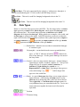
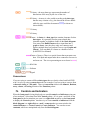
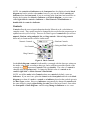
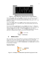
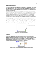
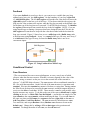
LabVIEW Reference
I.
LabVIEW Help
To access the LabVIEW help reference, click LabVIEW Tutorial on the startup box
(Find Examples is also a helpful resource with example VIs) or select Help >> VI,
Function, & How-To Help… from either the front panel or block diagram. There are
also LabVIEW manuals under Help >> Search the LabVIEW Bookshelf… for an
even more in-depth study of LabVIEW mechanics.
To access help on individual nodes of a VI, select Help >> Show Context Help to
display context help. Context help is a window that displays reference information for
the LabVIEW element near the cursor. It will help you figure out what each node does
and understand how the VI (LabVIEW code has a .vi extension) works when you are
trying to examine example code. It also contains a link to more information about the
element.
The LabVIEW help reference is an incredible resource for learning and understanding
LabVIEW mechanics. Included in the reference are a number of example VIs and many
step-by-step tutorials. You will most likely be able to find an example somewhere that
nearly implements the function you want to program using LabVIEW—the Internet is a
good resource as well. The LabVIEW help reference is nearly all you will need to learn
LabVIEW. This reference sheet will point out the things that LabVIEW can do and
describe some of its mechanics without the depth the LabVIEW help reference has.
II.
Interface
When you create a new VI, two windows will pop up. The first window is known as the
front panel and the second as the block diagram.
Front Panel
The purpose of the front panel is user-interface. On the front panel you will place the
controls, indicators, charts and graphs, etc. that the user needs to see and possibly use.
You can access the front panel from the block diagram by selecting Window >> Show
Panel.
You can align controls on the front panel using the Align Objects pull-down button on
the tool bar.
Block Diagram
The block diagram contains the meat of the program. Herein lie all the internal
workings and background operations of the code. On the block diagram you will place
nodes, wires, structures, etc. You can access the block diagram from the front panel
by selecting Window >> Show Diagram.
2
Palettes
To display a palette select Window >> Show [Palette Name] Palette. This will display
the palette in locked mode, which means that the palette will remain in that position until
it is closed (if you are using the controls palette and switch to the block diagram, the
controls palette will be closed and the functions palette opened.) Another way to
display the controls palette/functions palette is to right-click using any tool on either
the front panel or block diagram, and the corresponding palette will be displayed in
unlocked mode. When I direct you to Controls Palette or Functions Palette to access a
certain control or Function I will write it like Controls >> [Section] >> [Control
Name] or Functions >> [Section] >> [Function Name]. To change a palette to locked
mode, click the pushpin in the upper-left corner.
Pushpin
Figure 2. Controls Palette
Figure 1. Functions Palette
Figure 3. Tools Palette
Tools and Shortcuts
LabVIEW uses different tools to program your VI. These can be accessed from the
Tools Palette—if it is open—or by pressing tab until the tool you want is displayed as
3
the cursor (I have set the small button on the left side of the mouse in this lab as the tab
button to make this oft used task quicker). To display the Tools Palette, select Window
>> Show Tools Palette. Below is a description of the tools in the Tools Palette. From
this list, only the operate value, position/size/select, edit text, and connect wire tools
are available when using the tab key in the block diagram, and only the operate value,
position/size/select, edit text, and set color tools are available when using the tab key in
the front panel.
Automatic Tool Selection – This option is the top button of the Tools Palette.
It automatically selects the tools based on the context of the cursor location.
Operate Value – Use this tool to change the value of a control or constant, click on
buttons, switch between the frames of a structure, etc. This will be one of the tools—
along with the probe data tool—available when the VI is running.
Position/Size/Select – This is the tool you will use most often. Use it to position
nodes, move wires, resize structures and constant boxes, switch between the frames of
a structure, resize a node to include more input/output connectors, select a section of
code to copy it (with Ctrl | C), etc.
Edit Text – This tool edits any text in the VI, including values in a control or
constant (that aren’t symbolic), and case headings.
Connect Wire – This tool is only used on the block diagram. Use it to connect
nodes in the block diagram by selecting one output connector and one input
connector. When you place the connect wire tool over a node, the connector that you
are on top of will begin blinking. Also, if context help is open, the connector will blink
in that window as well. This will help you make sure to select the correct connector.
After you connect two connectors, one of two things will happen. Either a wire will
form between them color-coded with the data type it is carrying, or the wire will become
a dashed line. If the wire is a dashed line, this means that you have made an error.
Usually, the error will be that you connected two different data types or you connected
two input connectors (or two output connectors) together.
If you hold the connect wire tool over a wire, context help will show you what data
type is flowing through the wire. If you hold the tool over a dashed wire, a dialog will
appear describing the error that is causing the wire to be dashed.
Object Shortcut Menu – This tool is the same thing as a right-click using any tool
on either the front panel or block diagram. It displays the Controls Palette/Functions
Palette depending on whether you are in the front panel or block diagram.
Scroll Window – This tool has the same function as the hand in Adobe Acrobat: it
allows you to move around the front panel/block diagram by clicking and dragging.
Set/Clear Breakpoint – This tool, represented by the stop sign, is used for
troubleshooting the VI. Refer to the LabVIEW help reference.
4
Probe Data – This tool, represented by the circled ‘p’ with an arrow through it, is
used for troubleshooting the VI. Refer to the LabVIEW help reference.
Get Color – This tool is useful for changing background colors in the VI.
Set Color – This tool is useful for changing background colors in the VI.
III.
Data Types
Below is a list of the data types used in LabVIEW. The first image before each data
type represents a control on the block diagram, which outputs that data type (note
the solid outer line). The second image represents an indicator on the block
diagram, which inputs that data type. Both symbols are rectangles, color-coded, and
the data type is written on the inside. LabVIEW also draws an arrow on either the
right or the left side of these symbols to indicate if the symbol represents an input or
an output connector (e.g.
represents an output connector of the type double
and
represents an input connector of the type double).
Dashed Line: indicates an error either in mismatched datatypes
or connector types.
Polymorphic: means that this node can accept multiple data
types. A ‘POLY’ indicator in brackets,
, indicates an
array of any data type. It is the generic data type for most of
the array nodes.
Numeric: there are many numeric data types—unsigned integer,
signed integer, double, extended, complex, etc.—and you can
change the type of a numeric control, connector, or
indicator by right-clicking the control etc. >>
Representation >> [data type]. Non-integer data types are
color-coded orange (e.g.
types are color-coded blue.
) while integer data
Enum: is a special data type that allows you to assign values to
menu selections. After placing an Enum control, use the
edit text tool to change the name of the first item in the list.
Then, right-click >> Add Item After and type a name for
every additional item you want added to the list. To wire two
enum connectors together the items in each list must be
equivalent.
Boolean
Character String
5
1D Array: the array data type represents the number of
dimensions of the array by the size of the wire.
2D Array: An array is color-coded according to the data type
that the array consists of (e.g. the data on the left are double
while the type could also be numeric,
shown below).
, or cluster as
3D Array
4D Array
Cluster: A cluster is a data type that contains elements of other
data types. It is generally used to group related data
elements together to eliminate clutter on the block diagram.
You can use the Build Cluster node to input data into a
graph or chart, since they have only one connector and
require multiple data, but you don’t have to (see Graphs and
Charts). You can think of a cluster as a bundle of wires.
(LabVIEW User Manual)
Cluster of Arrays (There is a special cluster that represents error
data. File input and output nodes have connectors for error in
and error out. The wire representing an error cluster is
.)
File Path
Refnum
Signal
Conversions
If you are trying to connect different data types that are closely related, and LabVIEW
won’t let you, try using a conversion node (for example if you are trying to convert from
a character string to a file path). There are conversion nodes in the numeric, Boolean,
array, cluster, and string sections of the Functions palette.
IV.
Controls and Indicators
When the front panel is being displayed you can add controls and indicators using one
of two methods. Select them from the Controls palette—if it is open—and click on the
front panel at the location that you want it, or right-click anywhere on the front panel
to display the Controls palette. Another way to create controls or indicators from the
block diagram is to right-click on a node’s connector that you want wired to the
control/indicator >> Create Control or Create Indicator. You can also create
constants, which are manipulated only from the block diagram.
6
NOTE: the controls and indicators on the front panel are also displayed on the block
diagram and can be wired to other nodes; however, you can only delete controls and
indicators from the front panel; if you are working in the front panel and would like to
display the location of a control or indicator on the block diagram—or vice versa—
either right-click the control or indicator >> Find Control or Find Indicator or
double-click the control or indicator.
Controls
Controls allow the user to input information that the VI needs to do a calculation or
complete a task. They usually need to be changed by the user before the program runs or
updated on each cycle of a loop. There are five basic types of controls that you will use:
numeric, Boolean, string and path, list, and ring controls. List and ring controls
differ only in format and are used for similar tasks.
Numeric Controls
Boolean Controls
String and Path Controls
List Controls
Ring Controls
Figure 4. Basic Controls
On the block diagram a control is indicated by a rectangle with the data type written on
the inside, color-coded according to data type, and a solid line around the outside of the
rectangle (e.g.
represents a control of the type double). The value of a control is
changed using the operator tool. To change the default value of a control on the
control, right-click >> Make Current Value Default.
NOTE: not all the nodes in the Controls palette are controls by default: some are
indicators. If you aren’t sure, place the control on the front panel and look at the block
diagram to evaluate if a node is a control or an indicator, based on the symbols given in
the Data Types section. However, indicators can generally be changed to controls with
the same design by simply right-clicking the node after it has been created—from either
the front panel or block diagram—and selecting Change to Indicator or vice versa.
7
Indicators
Controls
Indicators
Figure 5. Numeric Controls Palette
Numeric Controls
Use numeric controls when a calculation needs to be performed or a decimal number is
required. Numeric controls are accessed from Controls >> Numeric >> [Control
Name]. The data type of a numeric control is numeric.
Boolean Controls
A Boolean control is a switch; it is either on or off, 1 or 0. The design of the Boolean
controls is generally in the form of push buttons or switch. Use these with case
structures, event structures, connected to a while loop’s conditional terminal, etc.
Boolean controls are accessed from Controls >> Boolean >> [Control Name]. The
data type of a Boolean control is Boolean.
Array Controls
Array controls are just like numeric controls only in an array format.
Graphs and Charts
Graphs and charts are accessed from Controls >> Graph >> [Graph or Chart Name].
They are used to display a plot of data. “Graphs and charts differ in the way they display
and update data. VIs with graphs usually collect the data in an array and then plot the data
to the graph, which is similar to a spreadsheet that first stores the data then generates a
plot of it. In contrast, a chart appends new data points to those already in the display. On
a chart, you can see the current reading or measurement in context with data previously
acquired.” (LabVIEW User Manual)
8
Figure 6. A Chart Displaying a Random Signal and a Digital Readout
If you feed a graph a 1D array, the graph will display the data with the values on the xaxis representing the index of the data element, beginning with zero. That is, if the
graph shows a point at (2,5), this means that the third number in the array is a five. The
same goes for charts.
If you feed a graph a 2D array, the graph will display multiple plots using the same
scheme as for a 1D array—i.e. the values on the x-axis will increment by one for each
element in the array.
You can also feed the graph cluster data using a Bundle node (Figure 7). Cluster the
initial x-value you want your graph to start with, the amount you want to increment x for
each point, and an array of y-values. This specific bundle (of x0, ∆x, y array) is
classified as WDT (waveform data type). The AI Acquire Waveform node, and other
nodes like it, outputs this type of data, so you can wire it directly to a chart.
Figure 7. WDT Bundle
V.
Mathematics
There are multiple ways of doing mathematic operations in LabVIEW depending on your
design intent. If you only need to do a few simple mathematical operations (add,
multiply, increment, etc.) use the operator nodes; you need to do some complex math or
a lot of operations at a time use either the formula node or the Matlab node (if you need
the functionality of Matlab).
Operator Nodes
Figure 8. An Example of a Mathematical Operation Using Operator Nodes
9
Figure 8 shows the operation (x+2)*(x2+1) using operator nodes, two numeric
controls—x and x2—and a constant—equal to 2.00. A numeric indicator displays the
result on the front panel. When the block diagram is being displayed you can place
operator nodes using one of two methods. Select them from the Functions Palette—if
it is open—and click on the front panel at the location that you want it, or right-click
anywhere on the front panel to display the Functions palette.
Arrays
You can use a for loop to build an array—see the section on for loops—or you can
initialize an array with Functions >> Array >> Initialize Array. The Initialize Array
node will initialize an array of the size you tell it (by wiring constants to the right
connectors) with the value you set in every index. Use the position/size/select tool to
make a higher dimension array by dragging the bottom of the node down to reveal more
connectors. You can also build an array by feeding many elements or arrays to the
Build Array node (Functions >> Array >> Build Array). If you are feeding the Build
Array node arrays, select whether you want the node to concatenate the arrays or not by
right-clicking on the node >> Concatenate Inputs. If you do not choose to concatenate
inputs, Build Array will add a new dimension to the output array (make sure all input
arrays have the same dimensions). For example, if you connect two 2D arrays to a build
array node, the node will output a 3D array if you do not concatenate inputs, but if you
select concatenate inputs, the node will output a larger 2D array.
Drag down to Create
Higher Dimension Array
Figure 9. Build Array and Initialize Array Nodes
Formula Node
Figure 10. An Example of a Mathematical Operation Using a Formula Node
Figure 10 shows the operation (x+2)*(x2+1) using a formula node, two numeric
controls—x and x2—and a constant—equal to 2.00. A numeric indicator displays the
result on the front panel. To add input or output variables to a formula node, right-click
the border of the node >> Add Input or Add Output. Then type a name for the variable
and wire it to the output connector of another node or a constant if the variable is an
input or an input connector of another node if the variable is an output. Now enter
mathematical statements you want the node to execute inside the node using the edit text
tool—end statements with a semicolon. The formula can do operations similar to those
used in C code.
10
Matlab Node
The Matlab node is just like the formula node except that a VI with a Matlab node in it
requires that Matlab be running in the background (open) in order operate correctly and
the statements must be written in the format of a Matlab script.
VI.
Programmatic Control
When you want to control how your program operates or the order of events use the
following techniques.
Sequential Control
Data Transfer
The first, obvious, form of control over the order of operations in LabVIEW is data
transfer. Before any node runs, it waits for data to be passed to all the connectors that
are wired. Therefore, any node which has an output connector wired to another node’s
input connector will complete its operation before the other node can begin. Any node
that has no input connectors wired will automatically operate as soon as the VI is started
(unless the VI contains another form of programmatic control, discussed in the following
sections).
Sequence Structure
Sometimes, however, you need two or more operations to happen sequentially even
though they are not wired together. To do this place a sequence structure on the block
diagram (Functions >> Structures >> Sequence). After picking the sequence
structure, drag out an area on the block diagram that the structure will take up.
Anything on the block diagram within the boundary of the sequence structure will be
included in the current frame of the sequence. At this point there is only one frame in
the sequence. LabVIEW will run only one frame at a time and move to the next frame
only after every node on the current frame has ended its operation. To add another
frame after this one, right-click on the border of the sequence structure >> Add Frame
After. A new, empty frame will be displayed, and all of the nodes on the first frame will
be hidden. Also, a heading is added to the structure. On the outsides of the heading are
arrows. Click on them to browse through the frames of the sequence. In the middle is
written the current frame number followed by the set of possible frames in the following
format: “1[0..1],” where 1 is the current frame and there are two frames, the first called
‘0’ and the second ‘1.’ In the blank space within the second frame (frame number ‘1’)
place the nodes that you want to operate after the first frame has completed. You can
continue to add more frames and code by right-clicking the border >> Add Frame
After or Add Frame Before whichever frame is currently displayed.
11
Sequence Local
Figure11. Frame 0 and Frame 1 of a Sequence
There will be times when you want to use sequence structures and data transfer at the
same time—i.e. pass data between the frames of a sequence. This is easily done by
creating sequence locals. Sequence locals are variables on the boundary of the
sequence that are available to all frames. Place one by right-clicking the boundary >>
Add Sequence Local. On one of the frames the data will be loaded into the sequence
local by wiring a node to that sequence local and then any of the nodes on the frames
after the frame from which the data is loaded can access that data by wiring from the
sequence local to an input connector on the correct node.
Repetition
For Loop Structure
To place a for loop select Functions >> Structures >> For Loop. After picking the for
loop structure, drag out an area on the block diagram that the structure will take up.
Anything on the block diagram within the boundary of the for loop will be included in
the for loop.
The for loop in LabVIEW operates just like a for loop would in another programming
language. In the top-left corner is a boxed ‘N.’ It is an input connector that accepts a
integer data type (represented by the color blue), and the loop will complete as many
iterations as the value wired to it. In the lower-left corner is a boxed ‘i.’ It is an output
terminal that also outputs an integer data type. Use this terminal to keep track of the
current iteration number—beginning at zero—or to do calculations with its value. The
loop will iterate as long as long as i<N.
Insert LabVIEW
Code Here
Figure 12. For Loop Structure
12
While Loop Structure
To place the while loop select Functions >> Structures >> While Loop. After picking
the while loop structure, drag out an area on the block diagram that the structure will
take up. Anything on the block diagram within the boundary of the while loop will be
included in the while loop.
Like the for loop, the while loop has a terminal in the lower-left corner (a boxed ‘i’)
which increments with each iteration, beginning at zero. The while loop, however, does
not have a boxed ‘N,’ because it operates not a specific number of times, but, instead,
until the conditional terminal receives a certain Boolean value. The conditional
terminal is in the lower right of the while structure, represented by either a boxed
circular arrow or a boxed stop sign. If the conditional terminal is a circular arrow,
then the while loop is set to run until a False, Boolean data type, is passed to the
terminal. If the terminal is a stop sign, the loop is set to run only as long as a False is
passed to the terminal. Change this setting by right-clicking the terminal >> Stop If
True or Continue If True. You must wire this terminal to some control for the VI to
run. If you want the loop to run forever simply right-click the terminal >> Create
Constant, and switch the constant to the correct value with the operate value tool.
Conditional Terminal
Figure 13. While Loop Structure
Tunnels
If you want a while loop or a for loop to build an array as it cycles simply wire a
number generator from inside the loop to outside the loop. Where the wire crosses the
boundary of the loop LabVIEW will create a tunnel. On the tunnel right-click >>
Enable Indexing, and the output will become the data type of a 2D array. (There is a
random number generator node in Functions >> Numeric.)
Figure 14. For Loop With a Random Number Generator Node
13
Feedback
If you want feedback in your loop: that is, you want to use a variable that your loop
updated on its last cycle, use shift registers. On the boundary of your loop, right-click
>> Add Shift Register. The left shift register will produce the value that was sent to the
right shift register on the last cycle of the loop. “If you do not initialize the register, the
loop uses the value written to the register when the loop last executed or the default value
for the data type if the loop has never executed.” (LabVIEW help reference) To initialize
the register, wire an input from outside the loop to the left register. NOTE: if you are
using nested loops or running a loop more than once during the time the VI is run, the
shift register will start the new loop with the value that it ended with the last time the
loop was executed. Figure 15 shows how to use a while loop with a Build Array node
to build an array using feedback. ‘Array’ is a control of the type 1D array, and ‘Array 2’
is an indicator of the type 2D array, because the Build Array node is not set to
concatenate inputs.
Shift Registers
Figure 15. Using Feedback in a While Loop
Conditional Control
Case Structure
“[The case structure] has one or more subdiagrams, or cases, exactly one of which
executes when the structure executes. Whether it executes depends on the value of the
Boolean, string, or numeric scalar you wire to the external side of the terminal or
selector.” (LabVIEW help reference) The case structure allows conditional control in a
VI—like an if-then statement. On the left side of the case structure is a question mark
terminal. Wire into this terminal any numeric, Boolean, or string data. During runtime
the VI will wait for data to be passed to the case structure, and then compare the data it
receives to the titles of each case. NOTE: There must be a case for each possible value
that the structure may receive. To do this, make one of the cases a default case by rightclicking on the case >> Make This Case the Default…, and in this case simply wire the
input tunnels to the output tunnels, without modifying the data. You can add cases in
the same way that you add frames in a sequence structure (right-click on the case >>
Add Case After or Add Case Before). The case structure by default has two cases,
True and False, and accepts Boolean values (Boolean case structures do not need a
default case). Change this by wiring a different data type to the question mark
terminal. To change the name of each case, use the edit text tool.
14
Figure 16. The Case Structure
VII. Input/Output
Files
The two most common methods of saving data in LabVIEW are in text format and
spreadsheet format. You can create a file in LabVIEW using either method and it will be
accessible to Excel. To create a spreadsheet file format, you must have data in array
form. Use the Write To Spreadsheet File node (Functions >> File I/O >> Write To
Spreadsheet File) and wire it to array data and a file path. The Write To Spreadsheet
File node also allows other functionality, such as appending to a file that already exists,
saving the data in a certain format that your spreadsheet program requires, etc.
Figure 17. Using Write To Spreadsheet File
To create a generic, text-based file is more difficult. First you have to place the New File
node on the block diagram (Functions >> File I/O >> Advanced File Functions >>
New File), or use the Open File node (Functions >> File I/O >> Advanced File
Functions >> New File) if the file already exists. Wire this node to a file path
control/constant. Next place the Write File node (Functions >> File I/O >> Write
File) on the block diagram, and wire the refnum output connector from the New File
node to the refnum input connector on the Write File node. Also wire in some data (of
any data type). Finally close the file using Close File (Functions >> File I/O >> Close
File), again wiring a refnum from the Write File to Close File. NOTE: these
operations will happen in the correct order because each node must wait until the
previous node sends it data—in the form of a refnum—if you wired the refnum from
the Open File node to the Close File node instead of from the Write File to the Close
File, the file may be closed before it is written (see the section on Data Transfer). The
Write To Spreadsheet File node does all of these steps for you.
15
Figure 18. Creating a File
ata Acquisition
To acquire data from the breakout boards use the Analog Input and Output nodes
found in Functions >> Data Acquisition >> Analog Input or Analog Output. You
will need to wire them the device number, usually 1, and the channel number, usually
0, using constants or controls (see the section on Controls and Indicators). The
Analog Input nodes will output the voltage it read from the specified input channel at
the time it ran, and the Analog Output nodes will output a voltage to some specified
output channel (reference the National Instruments breakout board reference card to
find which channels are input and which are output and where they are on the board).
You can also use the Acquire Waveform node and average the array it outputs with the
Mean node.
Constants
Figure 19. Using The Acquire Waveform Node