1
NUVIB 2 Northwestern University Vibration Analysis Program User’s Manual By: Kermin Chok Charles H. Dowding © Copyright Kermin Chok & Charles H. Dowding 2003 August 2003 Department of Civil and Environmental Engineering Northwestern University Evanston, IL 60208 TABLE OF CONTENTS 1 Introduction 1 2 Getting Started 2 3 2.1 Software required 2 2.2 Running NUVIB 2 3 2.3 Graphing in Excel 4 7 NUVIB 2 3.1 Overview 7 3.2 Input Data 9 3.3 Digitization of hardcopy data 10 3.4 Interpolation of data 14 3.5 Baseline correction 16 3.6 Integration of Time History 16 3.7 Fast Fourier Transform 17 3.8 Single Degree of Freedom (SDOF) Response Spectra 20 3.9 Single Degree of Freedom (SDOF) Relative Displacement Time History 22 3.10 Single Degree of Freedom (SDOF) Absolute Displacement Time 23 Air Blast Analysis 24 History 3.11 4 25 Theoretical Background 4.1 Interpolation 25 4.2 Baseline Correction 26 4.3 Integration 29 4.4 SDOF response spectra 29 4.5 Relative Displacement Time History 32 4.6 Absolute Displacement Time History 32 4.7 Air Blast Analysis 34 Appendix A: Example 1 (Blasting) 35 Appendix B: Example 2 (Blasting) 38 Appendix C: Example 3 (Earthquake) 40 Appendix D: Data processing for commercial seismic recorders 41 44 BIBLIOGRAPHY i LIST OF FIGURES Figure Figure Caption Page 1 Checking if “Analysis ToolPak” is installed 3 2 Delimiter Window in Excel 4 3 Chart Window 1 in Excel 6 4 Chart Window 2 in Excel 6 5 NUVIB 2 Main Window 5 6 NUVIB 2 Time History Data Processing Tab 6 7 Input Data Format 9 8 “List” Output in AutoCad 13 9 Processing of raw co-ordinates (Digitization of Hardcopy) 13 10 Interpolation Window in NUVIB 2 14 11 File Chooser Menu 15 12 Fourier Analysis Menu 18 13 Fourier Analysis Example 19 14 Frequency Plot Example 19 15 Selection of Frequencies for Analysis 21 16 Frequency Input File 21 17 Velocity Time History with Upward Offset 27 18 Displacement Time History with Upward Drift 27 19 Velocity Time History with Increasing Drift 28 20 Displacement Time History with Increasing Drift 28 21 Comparison of SDOF Spectra with Different Input Resolution 31 22 GEOSONICS Exported Digital Waveform 42 ii LIST OF EQUATIONS Equation Description of Equation Page 4.1 Linear Interpolation 25 4.2 Second Order Polynomial Interpolation 26 4.3 Integration by Trapezoidal Rule 29 4.4 Duhamel Integral 29 4.5 Trigonometric Relations 29 4.6 Modified Duhamel Integral 30 4.7 Equation for Free Vibration 30 4.8 Pseudo Velocity 31 4.9 Pseudo Acceleration 31 4.10 Equation for Single Degree of Freedom Absolute Displacement 32 4.11 Transformed Absolute Displacement Equation 32 4.12 Equation for Superimposed Pressure Time History 34 4.13 Equation for Acceleration 34 iii 1.0 INTRODUCTION NUVIB 2 is a program that facilitates the analysis of a single degree of freedom system subject to dynamic loading. It provides the all following functions in one user-friendly program. • Interpolation of data. • Baseline correction. • Integration of data. • Single Degree Spectrum Analysis. • Adjustment of data to perform Fast Fourier Transforms. • Relative Displacement Time History Analysis. • Absolute Displacement Time History Analysis. • Air Blast Data Processing. Graphs can be produced from the processed data by any spreadsheet program. The examples in this manual have been obtained with Excel. Active Excel files with processed data are included in this package to aid the learning process. 1 2.0 2.1 GETTING STARTED SOFTWARE REQUIRED In order to perform all the functions and analysis in NUVIB 2, the following is required. • Java Virtual Machine • NUVIB 2 • Microsoft Excel (or any commercial spreadsheet program with a Fourier transform function) • AutoCad Java Virtual Machine NUVIB 2 was written in Java2SE and in order the run the program, Java support must be available on the computer. It is likely that your computer already has Java support, but in case it does not, it can be obtained from: • http://java.sun.com/j2se/1.4.2/download.html: click on the download “JRE” link for your respective platform to install J2SE, JRE 1.4.2. or • From the NUVIB web site: download either the NUVIB 2 package containing the install file, or, if you already have the NUVIB 2 package, the install file alone. Save the file to some convenient location (or find it in the NUVIB 2 folder) and doubleclick to start the installation process. NUVIB 2 The NUVIB 2 package contains the following. • Nuvib2.jar (main NUVIB 2 program) • NUVIB 2 User Manual • Nuvib2.bat (batch file to start NUVIB 2) • Example files • (optional) install file for Java Virtual Machine NUVIB 2 can be run directly from the CD or a folder on your hard drive. Microsoft Excel Microsoft Excel or any commercial spreadsheet program is needed to perform graphing and Fourier Transforms. In particular, the “Analysis ToolPak” in Excel will need to be installed in order to access the Fourier Transform function. To check if the ToolPak is installed on the system, do the following. 1. Open Excel. 2. Click “Tools”. 3. Click “Add-Ins”. 2 4. Check if the box beside “Analysis ToolPak” is checked (Figure 1). 5. If the “Analysis ToolPak” is not installed, check the box and hit OK. Excel should then install the “Analysis ToolPak”. Figure 1: Checking if “Analysis ToolPak” is installed Should another Spreadsheet program be used, search for the Fourier Transform function in the program. This can usually be accomplished by clicking on help and typing “Fourier Transform” in the query box. AutoCad AutoCad will be used to perform digitization of hardcopy data. It will be used to “trace” a scanned image of the waveform and the vertices of the points on the waveform will be read from AutoCad. 2.2 RUNNING NUVIB 2 NUVIB 2 can be started simply by running the batch file (Nuvib2.bat) in the DOS command line or by double clicking on its icon in the windows environment. Nuvib2.jar and nuvib2.bat must be kept in the same folder for proper execution. 3 2.3 GRAPHING IN EXCEL The following section details how to plot data in Excel. Other spreadsheet programs should have very similar functions and capabilities. Graphing will be illustrated with a simple cosine function. One can easily read the period and amplitude of the function and thus check the correctness of the plot. The input file will be a .txt file to show the manner in which the Excel opens .txt files. Importing a .txt file 1. Start Excel. 2. Open “cosine (20hz).txt” provided with the NUVIB 2 package. 3. Select “Delimited” from the “Text Import Wizard” the hit “Next”. See Figure 2 for a screenshot of the “Text Import Wizard”. 4. Select “Tab” under “Delimiters” in the next menu. In the preview pane, the data should now have a line drawn between the two columns. 5. Hit “Finish” to import the data set. Figure 2: Delimiter Window in Excel Graphing Data 1. Click “Insert”, “Chart”. 2. Select “XY (Scatter)” and choose the type of chart you wish to have under “Chart sub-type”. Click “next”. 4 3. Check “columns” under “Series in”. Click the “series” tab to indicate where the relevant data is located. 4. Click “X Values” and select the data to plot in the X-axis. 5. Click “Y Values” and select the data to plot in the Y-axis. Note: the number of data points selected under the X & Y must be the same. 6. Hit “next”. “Chart Wizard – Step 3 of 4 – Chart Options” should now appear. Enter the “title”, “Value X axis” etc as desired. 7. Hit “next”. Select the desired location of the chart. Excel allows the user to place the chart on a new worksheet (tab) or as an object in the original worksheet. The former is better suited for printing while the latter for comparing two charts as two charts can be placed side by side on one worksheet for comparison purposes. 8. Hit “Finish” to obtain the final plot. 5 Figure 3: Chart Wizard window 1 in Excel Figure 4: Chart Wizard window 2 in Excel 6 3.0 3.1 NUVIB 2 OVERVIEW Upon running the program, a window as shown in Figure 1 will appear. This is the main window from which operations are chosen. The functions are arranged in the order that usual analysis is carried out. Figure 5: NUVIB 2 Main Window Upon selection of a particular tab, the right pane will switch to a pane containing one or two buttons with some text below it. A typical screen is shown in Figure 2. Figure 6: NUVIB 2 Time History Data Processing Tab A brief description of each tab and the operations under that tab follows in Table 1. 7 Time History Data Processing Perform Interpolation of Time History Interpolates raw data points to provide a data set with a constant time step. The program prompts the user for a desired time step and generates a data set with that time step via a first or second order polynomial. Procedure corrects for drift in a manually digitized data set. It allows for both linear and polynomial baseline correction. Perform Baseline Correction Integrate Time History Procedure performs numerical integration of data via the trapezoidal rule. Perform Integration SDOF Spectrum Analysis Perform SDOF Spectrum Analysis Procedure generates the response spectra of a single degree of freedom system via numerical evaluation of the Duhamel integral. Free vibration of the system after the end of ground excitation is accounted for in the analysis. Fast Fourier Transform (FFT) Adjust Data to 2n points Procedure pads data set with leading and trailing zeros to obtain a data set with 2n points. Actual FFT is performed in Excel. Relative Displacement Time History Perform Relative Displacement Time History Analysis Procedure generates relative displacement time history of system via numerical evaluation of Duhamel integral. Free vibration of system is evaluated up to twice length of input data. Absolute Displacement Time History Perform Absolute Displacement Time History Analysis Procedure generates absolute displacement time history of system via numerical evaluation of equation (4.9). Free vibration of system is evaluated up to twice length of input data. Air Blast Analysis Perform Air Blast Analysis Procedure generates three output files. The superimposed pressure time history, equivalent ground acceleration and velocity time history are computed from an input pressure time history data file. Table 1: Description of Functions 8 3.2 INPUT DATA FORMAT NUVIB 2 has been set up to read from.txt files. The format of input data has to follow a set format for error free running of procedures. The first column should read the time and the second column the value of data (e.g. ground velocity, acceleration etc). Shown in Figure 3 is an example of a cosine function with the required formatting. Time is indicated in the first column with the f(t) value in the second column. In the example, at time = 0 sec, f(0)=1. The delimiters (separators) between the two columns can be a space or a tab. Microsoft Excel automatically exports .txt files as tab delimited. Figure 7: Input Data Format 9 3.3 DIGITIZATION OF HARDCOPY DATA In situations where only hardcopies of ground motion is available, digitization of that record needs to be carried out. This section describes how to digitize a print out of a ground motion and format the data to work in NUVIB 2. AutoCad will be utilized to read co-ordinates off the hardcopy of the waveform. Scanning • Scan the waveform into Adobe Photoshop or any other imaging software (use as high a resolution as possible). • Save the file as a Jpeg or any other conventional image file. AutoCad Importing Image • Open a new AutoCad file. • Import the scanned image using the function “Raster Image”. This is located under the “Insert “ tab. Click “insert”, “raster image”. • Select the scanned file. • A new menu will pop up and all boxes should be checked except for the “rotation” box. • Hit “Ok” • AutoCad will ask for an insertion point in the command line. Hit “return” to place the image at the default (0,0) position. • AutoCad will ask for a scale factor in the command line. Hit “return” to scale the image at the default 1. • The image should now be at the origin at the original size with no rotation. Tracing Image • Switch the “OSNAP” function off. This can be done by typing “osnap” in the command line and switching “Object Snap” off. • Start a polyline. This can be done by typing “pl” in the command line. • Begin tracing the waveform by selecting points on the scanned image. For accuracy in the interpolation procedure later on, it is good to start the trace with a few points along the x (time) axis (zero values) before tracing non-zero y values. • Care must be taken not to select points too far apart and that points are consistently selected to the right of the last point (trace in the positive time direction only). For further accuracy, the peaks of the waveform should be captured in this trace. 10 • Hit “return” to end the polyline when the end of the waveform is reached. • Note the start and end time of the trace and also the peak y value (e.g. peak velocity = 19 in/sec). Obtain Co-ordinates • Select the completed polyline. This can be done by simply clicking on the line. • Use the “List” function. This can be found under the “Tools” tab, and “Inquiry”. A new window will pop up with the co-ordinates of the just drawn polyline. Click “Tool”, “Inquiry”, “List”. • Hit “return” a few times to get to the end of the list. • Under “Edit”, select “copy history”. This copies the text in the window. • Save the drawing and close AutoCad. Excel Import Text into Excel • Open Excel. • Paste the text into a new Excel spreadsheet. • Delete all rows not containing co-ordinate information. This can be done by selecting the relevant rows, choose “edit”, “delete”, “entire row”. • Separate text into columns. This can be done by selecting the rows, and clicking “data”, “text to columns” • The delimiter window should appear as in Figure 2. Select “fixed width”. Hit “finish”. This should separate the co-ordinates into different columns. If this does not work, select the “delimited” option, and select “tabs” and “space” as delimiters. • Delete all columns not containing co-ordinate information. Select columns, click “edit”, “delete”, “entire column”. • Co-ordinates should now be in two columns. Insert two rows above all the data and label the two columns “x” and “y” for easy reference. Manipulate Co-ordinate data • Create two new columns of data so the data set starts at 0,0. This can be done by subtracting the first value in the column from each raw data point. The data set should now start with 0,0. • Create another two columns of data that have scaled values. Scale the data by dividing the second column of data by the maximum value in that column. Use the “Max” function in Excel to identify the maximum value in the column. 11 • Multiply the previous value by the actual maximum value (e.g. max velocity = 15in/sec) read from the hardcopy of the waveform. • A complete set of data should now be obtained that represent the actual waveform. Plot the data and compare it against the original hardcopy to check whether any errors have occurred. Export Data To a .Txt File • Copy the final data to a new worksheet in Excel. • Use the function “paste special” to paste just the values and not the formulas you had used in the first worksheet. This can be done by “right-clicking” in the new worksheet , selecting “paste special” and choosing “values”. The new worksheet should now contain the final data set consisting of only numbers that will be analyzed. • Insert a row above the whole set of data. • Enter the number of data points (rows of data). • Export the worksheet as a .txt file. This can be done by selecting “file”, “save as”, under “save as type” choose “Text (Tab delimited) *.txt”. Enter a filename and hit “save”. • A data set containing the digitized waveform should now be available for analysis. 12 Figure 8: “List” Output in AutoCad Figure 9: Processing of raw co-ordinates (Digitization of Hardcopy) 13 3.4 INTERPOLATION OF TIME HISTORY Upon selecting “Perform Interpolation of Time History” in the main NUVIB 2 window, a smaller window will pop up with options to select the input data file and output data file. This window is shown in Figure 6. This is a typical window that pops up with the selection of each procedure. A functional description of each button follows. Figure 10: Interpolation Window in NUVIB 2 Set Input File: Sets the input data file. A file chooser menu (Figure 7) will appear and the file can be selected. Note: Default file filter is .txt as NUVIB 2 only operates with text files. Input data must conform to the format described in Section 3.2 “Input Data Format”. Set Output File: Sets the destination file for processed data. If a filename is entered that does not currently exist, NUVIB 2 will create a file by that name and extension. All files should have extension .txt for easy graphing and manipulation later on. Note: NUVIB 2 requires an output file to be set before a procedure is carried out. Perform Interpolation: NUVIB 2 prompts for a degree of polynomial to use. Enter linear (1) or second degree polynomial (2). Default interpolation procedure is a second degree polynomial. NUVIB 2 prompts for a desired time step. Default time step is 0.001 secs. Starts interpolation procedure. 14 Figure 11: File Chooser Menu A window informing that the procedure is complete will appear after computation is done. It will report that the procedure is complete, the number of points in the output data file, the time step utilized and the locations of the input and output files. 15 3.5 BASELINE CORRECTION NUVIB 2 corrects for both linear and second order drift in manually digitized data. Upon selection of “Perform Baseline correction” a smaller menu window similar to that in Figure 6 will appear. Selection of an input and output file is similar to that in Section 3.4 “Interpolation of Time History”. A brief description of the options available in the menu follows. The data to be baseline corrected should be plotted in Excel prior to baseline correction to visually identify the type of drift in the data. A linear and second order trend line can be plotted in Excel to help identify the type of drift to correct for. It should be noted that increasing the degree of polynomial to correct for does not necessarily result in a better output. Set Input File: Sets the input data file. A file chooser menu (Figure 7) will appear and the file can be selected. Note: Input data must have an equally spaced time step. Perform interpolation to create a data set of a constant time step. Set Output File: Sets the destination file for processed data. If a filename is entered that does not currently exist, NUVIB 2 will create a file by that name and extension. Note: NUVIB 2 requires an output file to be set before a procedure is carried out. Perform Baseline Correction: 3.6 NUVIB 2 prompts for a order of polynomial to fit to the data set. Default setting is a linear baseline correction. Starts Baseline correction procedure. INTEGRATION OF TIME HISTORY NUVIB 2 performs integration of time history utilizing the trapezoidal rule. This function is used to convert from acceleration time history data to velocity time history data and velocity time history to displacement time history data. A brief description of the options available in the menu follows. Set Input File: Sets the input data file. A file chooser menu (Figure 7) will appear and the file can be selected. Note: Input data must have an equally spaced time step. Perform interpolation to create a data set of a constant time step. Set Output File: Sets the destination file for processed data. If a filename is entered that does not currently exist, NUVIB 2 will create a file by that name and extension. Note: NUVIB 2 requires an output file to be set before a procedure is carried out. Perform Integration: Starts integration procedure. 16 3.7 FAST FOURIER TRANSFORM NUVIB 2 2n Data Adjustment NUVIB 2 adjusts data set so that the output data contains 2n (where n is an integer) points which will allow the Fast Fourier Transform procedure in Excel to be carried out. Input and output procedures are exactly the same as in Section 3.4 “Interpolation of Time History”. Excel will be utilized to perform the actual Fourier Transform. A brief description of the options available in the menu follows. Project Title: Enter a project title. Hit “return” to store this text. Set Input File: Sets the input data file. A file chooser menu (Figure 7) will appear and the file can be selected. Set Output File: Sets the destination file for processed data. If a filename is entered that does not currently exist, NUVIB 2 will create a file by that name and extension. Note: NUVIB 2 requires an output file to be set before a procedure is carried out. Perform Operation: Starts data adjustment procedure. Fourier Transform (Excel) The following section describes how to perform and analyze a Fourier Transform in Excel. • Import the padded data file. This data set should contain 2n points. • Select the “Fourier Analysis” tool. This can be found under “Tools”, “Data Analysis”, “Fourier Analysis”. A window like Figure 8 should appear. • Under “Input Range”, select the data to be transformed. Note: select only one column of data. Do not select the time column of data. • Under “New Worksheet Ply”, type in the name of the tab for the output data. • Hit “OK”. Excel will perform the Fourier Transform. 17 Figure 12: Fourier Analysis Menu Fourier Analysis The following section describes how to generate a meaningful frequency plot to identify the dominant frequencies in the waveform. In order to analyze the frequencies, the sampling rate (1/timestep) and the number of data points (k) must be noted from the input data. • Obtain the complex conjugate of each entry. In a new column, use the Excel function “IMCONJUGATE(cell)” to obtain the complex conjugate of the previous cell. • Compute the product of each pair of complex conjugates and divide by the number of data points. Power = [(Y x Conjugate)/ k]. Use the Excel function “IMPRODUCT (cell 1, cell 2)” and store the results of this in another column. • Normalize the “Power” values by dividing each “Power” by the maximum in that column. Store this in a column “relative Power”. • Create a column with header “counter” with entries 1 to k. • Compute the frequency multiplying the counter by the sampling rate divided by the number of points. Freq = [current counter/(timestep x k)]. • The final worksheet should resemble Figure 9. • Plot “relative Power” against “freq” to obtain the frequency domain of the waveform (Figure 10). • It is usually sufficient to plot the up to 25hz along the frequency axis since larger frequencies are seldom dominant nor meaningful. 18 Figure 13: Fourier Analysis Example Figure 14: Frequency Plot Example 19 3.8 SINGLE DEGREE OF FREEDOM RESPONSE SPECTRA NUVIB 2 computes the response spectra for a single degree of freedom (SDOF) system via numerical evaluation of the Duhamel integral. Free vibration of the system is taken into account in event that peak deformation occurs after the excitation of the system ends. Loading and saving of data is as Section 3.4 “Interpolation of Time History”. A description of the unique options available in this operation are detailed below. Project Title: Enter a project title. Hit “return” to store this text. Set Input File: A prompt for units of measurement will appear. Select the input units. Set the input data file. A file chooser menu (Figure 7) will appear and the file can be selected. Input data must be a ground velocity time history. Input data must have an equally spaced time step. For accuracy, time step should be greater than or equal 20 times the largest frequency analyzed.(e.g. if largest frequency analyzed is 100hz, time step should be 0.0005secs or less). Perform interpolation to create a data set with the desired time step. Set Output File: Sets the destination file for processed data. If a filename is entered that does not currently exist, NUVIB 2 will create a file by that name and extension. Note: NUVIB 2 requires an output file to be set before a procedure is carried out. Perform SDOF Analysis: A prompt for damping ratio will appear. Enter the damping ratio in % (e.g. 5). Default damping is 0%. Input frequencies for analysis (Figure 11). NUVIB 2 allows for analysis over a default range of frequencies or allows the user to input the frequencies for analysis. Starts computation of SDOF spectrum. Default Frequencies For Analysis If “Default Frequencies” is chosen, NUVIB 2 prompts for a largest frequency for analysis. The default frequencies are as follows. 2 – 20 : 2 Hz frequency step (e.g. 2, 4, 6, 8, 10…) 20 – 50 : 5 Hz frequency step (e.g. 25, 30, 35…) 50 – 90 : 20 Hz frequency step (e.g. 50, 70, 90) 90 – 100: 10 Hz frequency step (100) Input Frequencies For Analysis If “Read Frequencies from file” is chosen, NUVIB 2 will prompt for a file that contains the frequencies for analysis. A file chooser menu as in Figure 7 will appear. The frequencies for 20 analysis should be a .txt file and should contain the frequencies in rows with no header row. A “0” should be entered after the last row. An example of correct formatting for this file is shown in Figure 11. This file inputs frequency for analysis as 1 to 10 in 1Hz increments and a 0 is entered in the last row. Figure 15: Selection of Frequencies for Analysis 21 Figure 16: Frequency Input File 3.9 SDOF RELATIVE DISPLACEMENT TIME HISTORY NUVIB 2 computes the relative displacement time history for a given excitation via the numerical evaluation of the Duhamel integral. Free vibration is evaluated for twice the length of excitation. Loading and saving of data is as Section 3.4 “Interpolation of Time History”. A description of the unique options available in this procedure are detailed below. Project Title: Enter a project title. Hit “return” to store this text. Set Input File: A prompt for units of measurement will appear. Select the input units. Set the input data file. A file chooser menu (Figure 7) will appear and the file can be selected. Input data must be the ground velocity time history. Input data must have an equally spaced time step. For accuracy, time step should be greater than or equal 20 times the frequency analyzed.(e.g. if frequency analyzed is 100hz, time step should be 0.0005secs or less). Perform interpolation to create a data set with the required time step. Set Output File: Sets the destination file for processed data. If a filename is entered that does not currently exist, NUVIB 2 will create a file by that name and extension. Note: NUVIB 2 requires an output file to be set before a procedure is carried out. Perform Relative Displacement Time History Analysis: A prompt for damping ratio will appear. Enter the damping ratio in % (e.g. 5). Default damping is 0%. Input frequency for analysis. Default frequency is 5Hz. Starts computation of relative displacement time history. 22 3.10 SDOF ABSOLUTE DISPLACEMENT TIME HISTORY NUVIB 2 computes the absolute displacement time history of a system. Equations used for this computation is shown in Section 4.6 Absolute Displacement Time History. Free vibration is computed for twice the length of excitation. Loading and saving of data is as Section 3.4 “Interpolation of Time History”. A description of the unique options available in this procedure are detailed below. Project Title: Enter a project title. Hit “return” to store this text. Set Input File: A prompt for units of measurement will appear. Select the input units. Set the input data file. A file chooser menu (Figure 7) will appear and the file can be selected. Input data must be the ground displacement time history. Input data must have an equally spaced time step. For accuracy, time step should be greater than or equal 20 times the largest frequency analyzed.(e.g. if largest frequency analyzed is 100hz, time step should be 0.0005secs or less). Perform interpolation to create a data set with the required time step. Set Output File: Sets the destination file for processed data. If a filename is entered that does not currently exist, NUVIB 2 will create a file by that name and extension. Note: NUVIB 2 requires an output file to be set before a procedure is carried out. Perform Absolute Displacement Time History Analysis: A prompt for damping ratio will appear. Enter the damping ratio in % (e.g. 5). Default damping is 0%. Input frequency for analysis. Default frequency is 5Hz. Starts computation of absolute displacement time history. 23 3.11 AIR BLAST ANALYSIS NUVIB 2 provides the tools to perform preliminary calculations associated with Air Blast analysis. The three calculations it performs are: 1. Superimposed pressure time history. Psuperimposed = Pfront – Prear 2. Equivalent ground acceleration time history. a = Psuperimposed x C 3. Equivalent ground velocity time history. v = ∫ a dt where: P - pressure a - acceleration v - velocity C - pressure constant (A/m) A - Projected area m - system mass Section 4.7 “Air Blast Analysis” details the theory and execution of the above calculations. This procedure will output three separate data files. Loading and saving of data is as in Section 3.4 “Interpolation of Time History”. A description of the unique options available in this procedure are detailed below. Project Title: Enter a project title. Hit “return” to store this text. Set Input File: Set the input data file. A file chooser menu (Figure 7) will appear and the input file can be selected. Input data is a pressure time history. Input data must have an equally spaced time step. Perform interpolation to create a data set of a constant time step. Set Pressure Output File: Set Acceleration Output File: Sets the respective output files. A file chooser menu (Figure 7) will appear for each file and the file can be selected. Set Velocity Output File: Perform Air Blast Analysis: A prompt for time delay will appear. Enter the delay in secs. Default delay is 0 secs. A prompt for the pressure constant will appear. Enter the constant. The default constant is 1. It is important to ensure consistent units throughout these calculations. Start computation of output files. 24 4.0 THEORETICAL BACKGROUND OF NUVIB 2 This section details the equations and methodology used in NUVIB 2. 4.1 INTERPOLATION NUVIB 2 provides for both linear and second order polynomial interpolation. During the interpolation process, bounds are set such that the interpolated values are between the values of the raw data points. Linear Interpolation Linear interpolation is done by fitting a line between two data points and calculating values between them. y − y1 y= 2 ( x − x1 ) + y1 x2 − x1 (4.1) where: y - interpolated value at x x - current time yn - original data points Second Order Lagrange Interpolation NUVIB 2 performs a second order polynomial interpolation via the Lagrange interpolation procedure. This equation for this interpolation is shown in equation 4.2. Three data points (e.g. xi, xi+1, xi+2) are used during each calculation. Points are computed between the first (xi) and second raw data (xi+1) points and upon reaching the second data point (xi+1), the data points are advanced to the next set of three raw data points (xi+1, xi+2, xi+3) and interpolation is performed between the first two data points in that new set. Bounds that the interpolated values lie within the first and second point are set to preserve the frequency and shape of the original waveform (i.e. no artificial high peaks are generated). If the second order procedure results in points that do not lie between the first and second raw data points, linear interpolation is invoked to plot a straight line between the first and second point. The raw data points are then advanced and a second order polynomial is attempted between that next three raw data points. 25 n f n ( x ) = ∑ Li ( x ) f ( xi ) i =0 where (4.2) n x − xj j =0 j ≠i xi − x j Li ( x ) = Π 4.2 BASELINE CORRECTION Baseline correction is employed to correct for drift in a data set. This drift is usually attributed to inaccuracies in the scanning of a hardcopy waveform or problems with instrumentation. For analysis, it is usually best to work with a ground velocity time history that oscillates about zero. NUVIB 2 provides for linear and parabolic baseline correction. It is best to try to identify the type of drift inherent in the data set prior to attempting baseline correction. This can be done by plotting the raw velocity time history data and fitting both a polynomial and linear trend line to the data. The choice of linear or polynomial baseline correction can be made using the R2 value reported in Excel or examination of the equation Excel fits to the data. Linear Baseline Correction This corrects for increasing drift in the velocity time history data set. This shift is illustrated in Figure 17 where the velocity time history is offset by a linear function v = 2t + 0.1. Upon integration of this velocity time history, a displacement time history with parabolic drift is obtained (Figure 18). It would be highly inaccurate to analyze data with such a drift inherent. This type of drift in the velocity time history would be normally associated with an unintentional rotation and displacement of a scanned velocity time history waveform. NUVIB 2 corrects for such a linear drift by fitting a best-fit line (v = mt + c) to the raw velocity time history and proceeds to subtract this function from the original velocity time history. 26 Figure 17: Velocity Time History with Upward Offset Figure 18: Displacement Time History with Upward Drift Parabolic Baseline Correction NUVIB 2 provides for correction in event of a parabolic drift in velocity time history. This sort of drift is illustrated in Figure 19 where a parabolic function is added to a sin function. A second order trend line has been added to the graph to better illustrate the drift introduced. Upon integration of such a velocity time history, the displacement time history with a third order drift is obtained. It is noted that the original sine function is obscured by the disturbing parabolic function. 27 NUVIB 2 corrects for this problem by fitting a second order function to the velocity time history and then subtracting this function from the original velocity time history. Figure 19: Velocity Time History with Increasing Drift Figure 20: Displacement Time History with Increasing Drift 28 4.3 INTEGRATION NUVIB 2 performs integration of a data set via the trapezoidal rule. This method is shown in equation (4.3). The input to this procedure should be an interpolated data set (i.e. data set with constant time step). This is because NUVIB 2 reads the time step (dt) for integration as the difference between the times of two adjacent data points. This ensures n is always an integer. y = f ( x) with dt as a time step t ∫ [ f ( xn ) + f ( xn +1 )]dt 2 i =1 n −1 f ( x )dx = ∑ 0 where n = (4.3) t dt Problems with Numerical Evaluation With numerical evaluation, errors can be introduced via rounding and approximations of the actual waveform. Such errors can be substantially reduced with data sampled at a higher rate (smaller time step). Interpolation can be performed to obtain data at a higher resolution. 4.4 SDOF RESPONSE SPECTRA NUVIB 2 computes the SDOF response spectra via numerical evaluation of the Duhamel integral assuming velocity and relative displacement begins at zero at time zero. t . ξ u (t ) = − ∫ y (τ )e −ξωn ( t −τ ) cos (ω d ( t − τ ) ) − sin (ω d ( t − τ ) ) dτ 1−ξ2 0 (4.4) With the following trigonometric relations (equation 4.5), the above Duhamel integral can be transformed to equation 4.6. sin (ω d t − ω dτ ) = sin(ω d t ) cos(ω dτ ) − cos(ω dτ ) sin(ω dτ ) cos(ω d t − ω dτ ) = cos(ω dτ ) cos(ω dτ ) + sin(ω dτ ) sin(ω dτ ) 29 (4.5) t u ( t ) = − ∫ e −ξωnt eξωnτ 0 ξ cos(ω d t ) cos(ω dτ ) + sin(ω dτ ) . 1−ξ2 y (τ ) dτ ξ cos(ω dτ ) + sin(ω d t ) sin(ω dτ ) − 1−ξ2 (4.6) t . ξ e −ξωnt cos(ω d t ) ∫ eξωnτ y (τ ) cos(ω dτ ) + sin(ω dτ ) dτ 1−ξ2 0 u (t ) = − t . −ξωnt ξ ξω nτ sin(ω d t ) ∫ e y (τ ) sin(ω dτ ) − cos(ω dτ ) dτ +e 1−ξ2 0 where: . − − − absolute ground velocity − damped natural frequency natural frequency (Hz) ξ − − damping ratio wd − wn 1 − ξ 2 ωn − 2π f y u ωn ωd f relative displacement undamped natural frequency and: Equation 4.6 is used to calculate the relative displacement of a system during excitation and each of the integrals dτ is evaluated via the trapezoidal rule. Free vibration of the system is accounted for should the maximum deformation of the system occur after the end of ground excitation. This is evaluated using equation (4.7). u(t ) = e −ξωnt . u uo cos(ω d t ) + o + ξω n uo sin(ω d t ) ωd where: . u0 − velocity at end of ground excitation u0 − displacement at end of ground excitation 30 (4.7) NUVIB 2 evaluates equation (4.6) for the whole length of ground excitation and stores the maximum absolute value of displacement. The end displacement and end velocity of the system is transferred to equation 4.7 and this is evaluated for half the length of ground excitation. The maximum absolute displacement during free vibration is stored. The larger displacement between forced vibration and free vibration is obtained and reported as the deformation (D) of the system. NUVIB 2 also reports the Pseudo-velocity (V) and Pseudo-acceleration (A) of the system for each frequency evaluated. The formulas for V and A are shown in equation (4.8) and (4.9) respectively. V = 2πf D (4.8) A = (2πf)2 D (4.9) Problems with Numerical Evaluation Accurate evaluation of the Duhamel integral at higher frequencies require a higher sampling rate. The recommended sampling rate is twenty times the frequency to be analyzed. With insufficient resolution, an inaccurate response spectra illustrated in Figure 21 can result. It is generally expected that a SDOF response spectra resemble the blue line in Figure 21. Should a possible incorrect spectra illustrated by the red line result, the sampling rate of the input ground velocity should be increased (via interpolation) and the SDOF response spectra be recomputed. It should be noted that with increasing resolution, processing time for the computation of the SDOF response spectra would increase significantly. Figure 21: Comparison of SDOF Spectra with Different Input Resolution 31 4.5 SDOF RELATIVE DISPLACEMENT TIME HISTORY The computation of the relative displacement time history of a system is evaluated via the Duhamel integral (equation 4.6) in NUVIB 2. Equation (4.6) is evaluated for the whole period of excitation and for completeness, free vibration is evaluated for the length of ground excitation. Problems with Numerical Evaluation It is recommended that the sampling rate of the input data should be at least 10 times the frequency being analyzed. It has been generally noted that problems with numerical evaluation cease at sampling rates 20 times the frequency analyzed. Naturally, higher sampling rates increase computation times, although not significantly. 4.6 SDOF ABSOLUTE DISPLACEMENT TIME HISTORY Absolute displacement of a system may be approximated as u=x–y where: u - relative displacement of system x - absolute displacement of system y - absolute ground displacement NUVIB 2 computes the absolute displacement of a system more accurately via equation (4.10). t 1 − 2ξ 2 x (t ) = ω n ∫ y (τ )e −ξωn ( t −τ ) sin(ω d (t − τ )) + 2ξ cos(ω d (t − τ )) dτ 1 − ξ 2 0 (4.10) Using trigonometric relations in equation (4.5) and performing algebraic manipulation, equation (4.10) can be transformed to equation (4.11). t x (t ) = ω n ∫ y (τ )e −ξωnt eξωnτ 0 1 − 2ξ 2 sin(ω d t ) cos( wdτ ) + 2ξ sin( wdτ ) 2 1 − ξ dτ 2 1 − 2ξ sin( wdτ ) + cos(ω d t ) 2ξ cos(ω dτ ) − 2 1−ξ (4.11) t 2 −ξω n t ξωnτ 1 − 2ξ e sin(ω d t ) ∫ y (τ )e cos( wdτ ) + 2ξ sin( wdτ ) dτ 1 − ξ 2 0 x (t ) = ω n t −ξωnt 1 − 2ξ 2 ξω nτ cos(ω d t ) ∫ y (τ )e sin( wdτ ) dτ 2ξ cos(ω dτ ) − +e 1−ξ2 0 32 The absolute displacement time history is obtained via the numerical evaluation of equation (4.11) utilizing the trapezoidal rule. To provide a more complete time history of the system, free vibration of the system is evaluated via equation (4.7) for twice the length of ground excitation. Problems with Numerical Evaluation Similar to the computations of relative displacement time histories, it is recommended that the sampling rate of the input data should be at least 10 times the frequency being analyzed. Naturally, higher sampling rates increase computation times, although not significantly. 33 4.7 AIR BLAST ANALYSIS NUVIB 2 provides functions to compute a superimposed pressure time history, the equivalent ground acceleration and velocity time history. When an air blast acts on a structure, the structure first experiences a pressure on the leading side and after a delay experiences a negative pressure on its leeward side. A net superimposed pressure must be established for SDOF analysis to be performed. This is illustrated in equation (4.10). Ps (t ) = Pf (t ) t ≤ delay Ps (t ) = Pf (t ) − Pr (t − delay ) t > delay (4.12) where: Ps - superimposed pressure Pf - pressure on front of structure Pr - pressure on rear of structure Since a force acting on the mass of a SDOF is the same as force acting on its base (ground), an equivalent ground acceleration can be calculated from the superimposed pressure time history. The equivalent acceleration time history of the structure can be approximated by equation (4.13) F(t) = P(t)A a(t) = F(t)/m a(t) = P(t)A/m a(t) = P(t)C (4.13) where: F - force A - projected area of structure a - equivalent acceleration P - superimposed pressure m - mass C - pressure coefficient (A/m) The equivalent velocity time history of the system can be obtained by integrating the previously obtained acceleration time history. This integration is done utilizing the trapezoidal rule detailed in equation (4.3). 34 APPENDIX A: EXAMPLE 1 (BLASTING) In this appendix, a sample blasting ground motion is analyzed. The user could follow through the procedures and compare the obtained results to the provided file to checked for accuracy. All output has been processed and graphed for identification of trends and accuracy. The raw ground velocity data is provided as “Ex1.txt” and is located in the “Example 1” folder. All output .txt files have been included for the user’s convenience. All filenames associated with this ground motion end with Ex1 for easy reference and contain the following abbreviations to identify the data contained within. Abbreviation Description Interpolated Interpolated data file. A time history with a constant time step is contained. Linear baseline Linear Baseline corrected file. A velocity time history which oscillates about zero is obtained. Poly baseline Second degree Polynomial Baseline corrected file. A velocity time history which oscillates about zero is obtained. Poly with zeros SDOF The polynomial baseline corrected file with trailing zeros added to ensure zero ground velocity at end of record. First Single Degree of Freedom Spectrum. SDOF 2 Second Single Degree of Freedom Spectrum FFT File to perform Fast Fourier Transform with. The data set is padded with preceding and trailing zeros to obtain a data set with 2n points. RDTH Relative Displacement Time History. ADTH Absolute Displacement Time History. A detailed description of the steps performed for analysis now follows. The user should reference the output file “Example 1.xls” as they carry through this example. Data processing A manually digitized data set needs to be interpolated to obtain a data set with a constant time step. This constant time step allows error free computations in later operations. The data set also needs to be baseline corrected to correct for drift in the system. 1. Plot Raw Ground Velocity Time History Plot the digitized ground velocity and add linear and polynomial trend lines to identify any inherent drift in the data set. It is noticed that both linear and polynomial trend lines seem to “fit” the data set. Excel Tab: “Raw PR data” 35 2. Interpolation Interpolation on the raw data set is performed. A time step of 0.0005 secs was utilized in the interpolation procedure for this example. Excel Tab: “Interpolated PR” 3. Baseline Correction From the plot of the raw ground velocity time history, it was noticed that the trend in the data could fit either a linear or a second degree polynomial. As such, both a linear and polynomial baseline correction was performed separately. The plots of both data sets were compared and the polynomial baseline corrected data set was selected for analysis. The type of baseline correction to perform is a matter of judgement. Excel Tab: “Poly Baseline” (Tab contains the polynomial baseline corrected file with trailing zeros added) Excel Tab: “Linear Baseline” (Tab contains linear baseline corrected file and plots of both linear and polynomial baseline correction). Data Analysis 4. Ground Motion The polynomial baseline corrected file is integrated to obtain the ground displacement time history. Input file: “poly with zeros”. Excel Tab: “Ground Motion”. 5. SDOF Response Spectrum The SDOF response spectrum is computed for a range of frequencies. A plot of Pseudo-Velocity against Frequency can be obtained and it is noticed that system response is noticeably higher at approximate natural frequencies of 14hz, 25Hz, 30Hz and 45Hz. It should always be checked that the spectrum follows the general trend that is expected for response spectrums (i.e. An initial upward slope with a few peaks, the highest peak then a general downward trend.). If it is noticed that the obtained response spectrum follows an upward trend throughout the range of frequencies, a smaller time step should be used in the interpolation procedure. With trial and error, it was noticed such numerical errors ceased at sampling frequencies twenty times that of the frequency being analyzed (thus the default interpolation time step of 0.0005secs). Input file: “PR poly with zeros”. Excel Tab: “SDOF Spectrum”. 36 6. Fourier Frequency Analysis The input data is adjusted to contain 2n data points. In this instance, the final data set contains 2048 data points and n equals 11. Input file: “poly with zeros”. Excel Tab: “FFT Ex1”. The Fourier Transform is performed in Excel. The steps to obtain the “power” and respective frequencies are described in Section 3.7: Fourier Analysis. A plot of the relative power against frequency is obtained in this worksheet. The dominant frequencies in the spectrum are marked out and noted. Excel Tab: 7. “Fourier Analysis”. SDOF 2 A second SDOF spectrum is computed with a range of frequencies that include the dominant frequencies identified from the Fourier analysis. It is noted that the peaks in the SDOF spectrum closely math those in the Fourier Analysis. Input file: “poly with zeros”. Input file (freq): “Freq Ex1”. Excel Tab: 8. “SDOF 2”. Relative Displacement Time History The relative displacement time history of the system is computed. An arbitrary damping ratio of 5% and natural frequency of 5hz was entered in the computation process. Input file: “poly with zeros”. Excel Tab: “Relative Displacement Time History”. 9. Absolute Displacement Time History The absolute displacement time history of the system is computed. An arbitrary damping ratio of 5% and natural frequency of 5hz was entered in the computation process. A plot of the ground motion is included on the worksheet to identify any correlation between the ground motion and the motion of the structure. Input file: “grd disp Ex1”. Excel Tab: “Absolute Displacement Time Hist”. 37 APPENDIX B: EXAMPLE 2 (BLASTING) This appendix provides another complete example from interpolation to SDOF analysis for a given blasting ground velocity time history. The ground motion data illustrated can be found in the folder “sample file > raw sample data”. The ground motion is provided as “1 sampledata.txt”. This is the original ground velocity data as digitized manually. All output has been processed and graphed and all this can be found in the file “Example 2.xls”. This is an active excel file which can be manipulated and used as a template for future analysis. It is recommended that all desired changes be made to a copy of the original file. Due to the number of worksheets/tabs included in this file, a complete listing and description of all tabs are provided below. Tab Description Filename Sample data Original digitized ground velocity. Note: A non constant 1 sampledata.txt time step is present due to the manual digitization process. Interpolated raw Interpolation is performed on the original data set. Time step 2 interpolated raw sample data used was 0.0005s. A plot with a trend line added reveals that sample data.txt an upward shift in the time history exists. Linear Baseline Linear baseline correction is performed on the original data 3 linear baseline samp data set. Note: ground velocity now oscillates about zero. corrected raw sample data.txt Ground Motion The baseline corrected time history is integrated to obtain the 4 grd motion sample samp data ground displacement time history. Note: A non-zero ground data.txt displacement at end of time history exists. This is due to nonzero velocity at end of velocity time history. This can be corrected by the introduction of trailing zeros at the end of the waveform. Sample data Original data with a linear function added. This linear with drift function was added to better illustrate the linear baseline 1 Ex2 with drift.txt correction function in NUVIB 2. Note: The data is plotted and it is clearly noticeable that an upward drift in the data exists. Interpolated data Interpolation on the data set with drift introduced is with drift performed. A time step of 0.0005s is used. Linear baseline Data set with linear baseline correction performed. The 38 2 interpolated Ex2.txt 4 linear baseline Ex2.txt corrected velocity time history is now observed to oscillate about zero. This is plotted and compared to the original data set after baseline correction. Ground disp The linear baseline corrected file is integrated to obtain the 4 grd displacement ground displacement time history. The result is comparable Ex2.txt to the ground motion obtained from the original data set. SDOF analysis Single Degree of freedom analysis on the ground velocity 5 SDOF Ex2.txt time history is performed. A graph of Pseudo-Velocity against Frequency is plotted. Peaks in the SDOF spectrum are noticed at 10hz and 18hz. Padded data The data set is adjusted to contain 2n (where n is an integer) 7 FFT Ex2.txt data points to allow the Fast Fourier transform procedure in Excel to be carried out. It was necessary to truncate the data set as Excel only handles FFT of data with less than 4096 points. With 4096 adjusted data points, n = 12. Fourier Analysis The results from the Fourier transform on the adjusted data In excel file set is performed. The necessary operations to identify the dominant frequencies contained in the data set is performed and illustrated. A plot of the relative power against frequency is included. The dominant frequencies are identified as approximately 10hz and 18hz, as expected from the SDOF spectrum. Relative Disp The relative displacement time history of a 5hz system is Time History computed for the ground motion. A damping ratio of 5% is 6 RDTH Ex2.txt assumed. Abs disp time The absolute displacement time history of a 5hz system is history computed. A damping ratio of 5% is assumed. 39 8 ADTH Ex2.txt APPENDIX C: EXAMPLE 3 In this appendix, an earthquake ground motion is analyzed. This example provides the user with a complete example from manual digitization of a ground acceleration time history to dynamic analysis. These files can be found in the “Example 3” folder. A complete listing and description of each file follows. Filename Description 1 Raw accel Ex3 .txt Raw digitized acceleration data. 2 interpolated Ex3 .txt Interpolated acceleration data. Note: Time step used was 0.0125secs. It was possible to use this significantly larger time step (compared to in analysis of blasting ground motion) since the maximum frequency for SDOF analysis would be much smaller than in a blasting ground motion. 3 linear baseline Ex3 .txt Linear baseline corrected acceleration data. Note: Acceleration is calculated in “g”s. 4 grd vel Ex3 .txt Integrated acceleration data giving ground velocity. 5 SDOF Ex3 .txt SDOF Spectrum. 6 SDOF 2 Ex3 .txt Second SDOF spectrum with different range of frequencies. 7 FFT Ex3 Padded velocity data with preceding and trailing zeros added to obtain a data set with 2048 (211) points. Freq Ex3 .txt Frequencies utilized in SDOF 2. Example 3.xls Excel file with complete computation and graphs. Processing of digitized data Ex3 .xls Excel file with procedures to convert co-ordinates obtained from AutoCad to meaningful data. Ground Accel Ex3 .dwg AutoCad file with polyline included. Ground Accel Ex3 .jpg Scanned image of original waveform. There is no significant difference in the procedure for analysis of system response from a blasting ground motion or an earthquake ground motion. The only significant differences in general would be the length of the input data set (since earthquake ground motions in general last relatively longer than blasting ground motion) and the dominant frequencies (much lower dominant frequencies) within the spectrum. The length of the data set and generally lower dominant frequencies hint that a larger time step for interpolation should be used (for computational purposes). A time step of 0.0125secs, contrast to 0.0005secs in pervious examples, was employed in this analysis and the output conforms to the general behavior that we expect. Thus this larger time step was acceptable. 40 APPENDIX D: DATA PROCESSING FOR COMMERCIAL SEISMIC RECORDERS Ground motion data from commercial seismic recorders generally do not come in a format that NUVIB 2 can process. This appendix details how to extract and format data from commercial seismic recorders to work in NUVIB 2. The commercial programs NOMIS and GEOSONICS will be used to illustrate this procedure. GEOSONICS This section will detail how to export and process data from GEOSONICS. Export Ground Motion Data 1) Start GEOSONICS. 2) Open folder for analysis. 3) Select time history for analysis. 4) Export Data. Click “Export Data”, “Digital Waveform with Header”. Processing of Exported Data 1) Start Excel. 2) Open a blank worksheet. 3) Import Data. Click “Data”, “Get External Data”, “Import Text File”. 4) Select the data file. Select “All Files” under “Files of type” to be able to choose the .WFM GEOSONICS file. 5) Select “space” as under the “Delimiters” window (refer Figure 2). 6) Hit “Finish”, “ok”. Data should now resemble Figure 21. Formatting of Data to NUVIB 2 Format 1) Make a copy of the worksheet in Excel. Right click on the tab at the bottom of the worksheet, select “Move or Copy”, “Create a copy”. 2) On the copy of the data, note the length of record. This can be read from the header in the file e.g. “Record Time: 5 s”. 3) Delete the rows and column of no interest. 4) Determine the time step in the record. Time step = length of record/number of points. 5) Insert a column to the left of the ground motion data to include a time counter in the record. Click “Insert”, “Columns”. 6) Enter the time in the created column, starting from time step. 7) Insert a header row at the top with entries (0,0) to start the ground motion record. 41 8) Export the processed worksheet. Select the worksheet containing the processed data, click “File”, “Save As”, select “Text (Tab delimited)” under “Save as type”, enter desired filename, hit “Save”. 9) The data file should now be in the correct format (refer Figure 7) as a .txt file. Figure 22: GEOSONICS Exported Digital Waveform 42 NOMIS This section details how to export data from NOMIS to a .txt file. Exporting NOMIS data to .txt 1) Start NOMIS. 2) Navigate to respective folder. 3) Select the file. 4) Click “Data Analysis”, “Convert to Text Files”. 5) Select the desired destination folder. 6) Hit “Begin Conversion”. The file should now be exported to the specified folder as a .txt file. The processing and formatting of data to be used in NUVIB 2 can be done as directed in the GEOSONICS section above. Note: The delimiters during the import process should be “Fixed width” and not “space” as with GEOSONIC data. 43 BIBLIOGRAPHY CHOPRA, A.K. (2001), “ Dynamics of Structures: Theory and Application to Earthquake Engineering”, 49pp. CHAPRA, S.C., and Canale, R. P. (2002), “Numerical Methods for Engineers (4th edition)”, 444pp. DOWDING, C. H. (2000), “Construction Vibrations”. HUDSON, D.E. (1979), “Reading and Interpreting Strong Motion Accelerograms”. VELESTOS, A. S., and NEWMARK, N. M., (1964), “Response Spectra of Single Degree of Freedom Elastic and Inelastic Systems”. 44