Download Dynamic Structural Analysis Suite (DSAS) User Manual

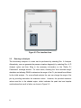
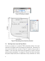
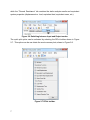
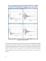
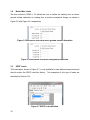
CIPPS TR-002-2012
Dynamic Structural Analysis Suite (DSAS)
User Manual
Version 4
Serdar Astarlioglu and Ted Krauthammer
March 2012
Acknowledgements
The Center for Infrastructure Protection and Physical Security would like to thank the
US Army Engineer Research and Development Center at the Waterways Experiment
Station in Vicksburg, MA and the Defense Threat Reduction Agency for their partial
support to perform this research code and development.
Contents
1
Introduction .............................................................................................................. 1
1.1
Installing DSAS .................................................................................................. 1
1.1.1
2
System Requirements ................................................................................. 1
1.2
Installation Instructions ....................................................................................... 2
1.3
Installing License................................................................................................ 2
Running DSAS ......................................................................................................... 4
2.1
Starting a New Analysis ..................................................................................... 4
2.2
Activating Visualizer ........................................................................................... 4
2.3
Running an Analysis .......................................................................................... 5
2.4
Switching between Input and Output Modes ...................................................... 6
2.5
Analyzing Rectangular Reinforced Concrete Beams/Columns ........................ 10
2.6
Analyzing Round Reinforced Concrete Columns ............................................. 15
2.7
Analyzing Steel Beams/Columns ..................................................................... 16
2.8
Analyzing Masonry Block Walls ....................................................................... 17
2.9
Analyzing Masonry Brick Walls ........................................................................ 17
2.10 Analyzing Reinforced Concrete Joists .............................................................. 18
2.11 Analyzing Reinforced Concrete Slabs .............................................................. 19
2.12 Analyzing Reinforced Concrete Boxes ............................................................. 22
2.13 Analyzing Wood Panels ................................................................................... 24
2.14 Analyzing User Defined Systems ..................................................................... 25
2.14.1 Simple Version .......................................................................................... 25
2.14.2 Advanced Version ..................................................................................... 26
3
Loading Options ..................................................................................................... 30
3.1
ii
Point Load ........................................................................................................ 30
iii
3.2
Uniform Load.................................................................................................... 30
3.3
Air Blast Loads ................................................................................................. 32
3.4
Buried Box Loads ............................................................................................. 33
3.5
SDOF Loads .................................................................................................... 33
1
Introduction
Dynamic Structural Analysis Suite (DSAS) is a multifunctional structural analysis
program capable of modeling the response of a wide range of structural components
under static or dynamic loads. DSAS has been in development under the direction of
Dr. Krauthammer since 1979. The current version is written in C# using object oriented
programming principles and supports the latest operating systems and processor
technologies. The component library includes reinforced concrete beam, column, and
joists, steel beams and columns, CMU and brick masonry walls, reinforced concrete
slabs and boxes, wood panels, and simple or advanced mass-damper systems. In
addition to performing time-history analysis, DSAS can generate the moment-curvature
and resistance (load-deflection) functions for the beam and column type components.
DSAS has built-in capability to generate the pressure-impulse or load-impulse diagrams
for any of the components mentioned above.
DSAS’s diverse program capabilities
enable it to be used as a sophisticated design evaluation tool. Since the simulations are
performed in only a matter of seconds the program is well suited for an iterative design
procedure. Use the increasingly sophisticated levels of analysis to refine your design.
1.1
Installing DSAS
1.1.1 System Requirements

Supported Operating Systems: Windows XP, Windows Vista, Windows 7,
Windows Server 2003, and Windows Server 2008

Processor: 400 MHz Pentium processor or equivalent (Minimum); 1 GHz
Pentium processor or equivalent (Recommended).

RAM: 98 MB (Minimum); 256 MB (Recommended).

Hard Disk: 2 MB of available space for DSAS. (Up to 500 MB of available space
may be required for .NET Framework if it is not already installed).

Display: 800 x 600, 256 colors (Minimum); 1024 x 768 high color
(Recommended).

Microsoft .NET Framework 3.5 or later. If DSAS setup does not detect .NET
Framework during installation, it will direct to user to the Microsoft website for
download. See Section 2.2 – Step 2a.
1

DPlot or DPlot Jr. version 2.1.5.0 or later. Without a current version of DPlot, the
analysis results cannot be plotted.
1.2
Installation Instructions
1. Download and save DSAS setup file to a common location such as Desktop or a
temporary installation folder as shown in Figure 1-1.
2. Double click on the setup file to start installation. It may be necessary to login as
admin if the current user has limited read/write permissions.
a. If .NET Framework is not installed, the setup will direct to Microsoft web
site. Select the link labeled “Get the .NET Framework 3.5” link. Follow
the instructions on that page for installing .NET Framework. After the
>NET Framework is installed, double click on DSAS setup to restart
installation.
3. Select the installation folder (Default is C:\Program Files\DSAS\) and make sure
“Everyone” is checked. Select “next” and follow the on screen instructions.
Figure 1-1 DSAS Installer
1.3
Installing License
1. From Start All Programs  DSAS select DSAS.
2
2. If there is no existing license file, you will receive an error message titled
“License file was not found”. Click OK.
3. After DSAS loads, select Tools  License  Create License Request.
Figure 1-2 Creating the license file.
4. Save the license file (License.Xml) to a common location such as Desktop.
5. Email the License.Xml file to Serdar Astarlioglu ([email protected]).
6. Serdar will email a signed “License.Xml” file. Save this file to a common location
(you can overwrite the original one you created).
7. Start DSAS.
8. Select: ToolsLicenseImport License File, open the License.Xml file you
received.
Figure 1-3 Importing the license file.
9. DSAS should restart automatically and all the menu options should be available.
3
2
2.1
Running DSAS
Starting a New Analysis
A new analysis can be started by selecting the desired component from the File  New.
Figure 2-1 Starting a new analysis.
2.2
Activating Visualizer
The visualizer can be activated by selecting View  Visualization as shown in Figure
2-3. The visualize form, shown in Figure 2-3 shows the loading and support information
in addition to cross-section details and is updated as new rebar layers or dimensions
are modified. The visualizer can be used with all the component types in DSAS.
Figure 2-2 Activating visualizer.
4
Figure 2-3 The visualizer form.
2.3
Running an Analysis
The time-history analysis of a case can be performed by selecting Run  Analysis.
Alternatively, one can generate the pressure-impulse diagram(s) by selecting Run  PI
Analysis option and then filling in the necessary information on the “Define P-I
Parameters” message window. For most cases, checking the “Auto calculate range”
checkbox and allowing DSAS to determine the range of the P-I plot should be sufficient
for the initial analysis. For more refined analysis, the user can change the range of the
plot by providing alternative the maximum values. However, the provided maximum
values must be in the shaded region, which indicates the peak load and impulse
combinations that result in failure, as shown in Figure 2-5.
5
Figure 2-4 Running an analysis.
Figure 2-5 Specifying pressure-impulse parameters.
2.4
Switching between Input and Output Modes
As soon as an analysis run is completed, DSAS automatically switches to the output
mode with all the analysis results are arranged into individual tabs. Alternatively, the
user can use the Mode menu, as shown in Figure 2-6, anytime as long as output is
available. In the output mode, all the results are presented in a number of tabs and
each tab contains a spreadsheet. For example, the “Flexural Time-History” tab contains
the dynamic analysis results (time vs. displacement, velocity, acceleration, etc. values)
6
while the “Flexural Resistance” tab contains the static analysis results and equivalent
system properties (displacement vs. load, equivalent load, equivalent mass, etc.).
Figure 2-6 Switching between Input and Output modes.
The quick plot option can be activated by selecting the DPlot toolbar shown in Figure
2-7. This option can be use obtain the most common plots, shown in Figure 2-8.
Figure 2-7 DPlot toolbar.
7
Figure 2-8 Plots in DPlot.
The user can select multiple columns by clicking on the column headers while pressing
control button and copy the contents of the selected columns into the clipboard by rightclicking and selecting copy from the context menu. Alternatively, the copy button on the
toolbar or the shortcut Ctrl+C can be used. The Plot command is limited to plotting two
columns against each other while Copy command can be used on any number of
columns.
8
Figure 2-9. Copying/plotting output
Figure 2-10 General information for rectangular reinforced concrete
beams/columns
9
2.5
Analyzing Rectangular Reinforced Concrete Beams/Columns
For rectangular shaped sections, the “General” tab, shown in Figure 2-10, contains the
geometric properties of the beam, the list of rebar layers, and transverse reinforcing
information. Additional rebar layers can be added by clicking on the add (+) button or
existing rebar layers can be removed by first selecting the desired row by clicking on the
row header and then clicking on remove (X) button.
The rebar layer depths are
measured from the face of the member that is exposed to load to the center of the
rebar.
The effect of diagonal shear on the flexural capacity of the section can be included
(recommended) by selecting the “Include effect of diagonal shear” check box.
The “Materials” tab contains the material properties for the concrete, longitudinal steel
and transverse steel. The detailed concrete properties can be accessed by clicking on
the “Concrete Details” button, as shown in Figure 2-11.
Figure 2-11 Materials tab and editing concrete properties.
10
The longitudinal and transverse steel properties can be edited by clicking on “Long.
Steel Details” and “Trans. Steel Details” buttons, respectively. As shown in Figure 2-12,
the user has the option of selecting between an elastic perfectly plastic (EPP) and strain
hardening models (Hardening). In the latter case, additional material properties such as
ultimate strength, strain hardening initiation strain must be supplied
Figure 2-12 Materials tab and editing steel properties.
The loading and boundary tab, shown in Figure 2-13 for beams and in Figure 2-14 for
columns, allows the user to define the type of the load, the load function, and the
boundary conditions at each end. It is also possible to specify static axial load for
beams (compression > 0). For column type members, the user can specify additional
time-dependent axial loads in addition to the static gravity load. When pressure loads
11
are applied, DSAS by default assumes the tributary width to be the overall width of the
member, however, the user can check the “Loads applied indirectly” box and specify a
different tributary width and additional superimposed loads for mass calculation.
Figure 2-13 Loading and boundary tab for beams.
Figure 2-14 Loading and boundary tab for columns.
The parameters for time-history analysis can be set from the Analysis tab. The user
can specify different runtime (duration of the analysis), damping values, time step
intervals for saving the data points (For example Output Interval = 10 saves the
displacements, velocities, etc at every 10th time step. Setting Output Interval = 0 saves
every time step). The time step size is automatically determined by DSAS based on the
component’s period and/or load rise time.
The user can modify the criteria for
calculating time step size by clicking on the “Advanced” button and selecting a different
12
period to time step size (
) and rise time to time step size (
). However, caution
must be exercised when changing these defaults.
Figure 2-15 Analysis tab and setting time-integration parameters.
The failure criteria option can be used to stop the analysis if a critical displacement,
velocity, or acceleration value is reached. The default selection is “None” and in this
case the analysis will carry on till the material failure.
If instead of “None”,
“Displacement” is selected and the “Value” is set to the yield displacement, the analysis
will stop when the component yields. The “Failure Criteria” setting is also preserved
when running P-I analysis. For example, running a P-I analysis when the failure criteria
is set to the yield displacement will plot the P-I diagram for pressure and impulse
combinations that cause the component to yield not to fail (which would be the case if
“None” was selected).
13
The dynamic load effects on the materials can be specified by clicking on the “Edit”
button next to the “Dynamic Increase Factors” label on the “Analysis” tab and providing
the necessary information on the dialog box shown in Figure 2-16.
Figure 2-16 Dynamic increase factors.
The moment-curvature plot options can be modified by clicking on the “Edit button next
to the “M-φ Plot Options” label on the “Analysis” tab. The values shown on Figure 2-17
are the default values DSAS uses when performing flexural analysis of the section.
DSAS will obtain the moment-curvature function of the section until the final moment
capacity drops to a fraction of the ultimate moment capacity (default is 0.10, meaning
10%) or it reaches maximum curvature value, φMax (default is 0.03). If after performing
an analysis, the moment-curvature curve does not exhibit any descending branch or
drop in capacity at φMax, then this value should be increased and the analysis should
be re-run.
14
Figure 2-17 Moment-curvature plot options.
2.6
Analyzing Round Reinforced Concrete Columns
The “General” tab for round columns is slightly different than that of rectangular cross
sections as shown in Figure 2-18. Instead of rebar layers, the bar size and the number
of bars should be provided. The tabs for defining materials, loading and boundary
conditions, and analysis parameters are the same as the rectangular case.
Figure 2-18 General tab for round reinforced concrete columns.
15
2.7
Analyzing Steel Beams/Columns
Figure 2-19 shows the “General” tab for a steel beam/column with a wide flange section.
Figure 2-19 General tab for steel beams/columns.
The user can either select a standard AISC section from the drop down menu or define
a custom section by checking the “Built-up section” checkbox and clicking on “Define”
button to enter dimensions. The loads can be applied in either strong-axis direction or
weak-axis direction.
There are three different lateral bracing options: continuous,
unbraced, and specify. If specify is selected, the user needs to provide the braced
length (Lb). If unbraced is selected, the unbraced length is taken as the entire length of
the member. The material properties can be edited by clicking on the “Steel” button.
The “General” tabs for steel channels and tubes are essentially the same and each are
16
connected to AISC channel and tube databases. The loading and boundary conditions
and analysis tabs are as described previously.
2.8
Analyzing Masonry Block Walls
Figure 2-20 shows the “General” tab for masonry block walls. The user can select
between grouted and ungrouted sections by checking the “Grouted” checkbox. For fully
grouted sections, the grout spacing should be provided as zero. Similarly, reinforcing
can be specified by providing the bar size and spacing. The equivalent resistance and
mass of the wall are calculated per unit width (=1 in).
Figure 2-20 General tab for masonry block walls.
2.9
Analyzing Masonry Brick Walls
The masonry brick wall module is suitable for analyzing two-wythe or single-wythe
masonry walls. For two-wythe walls, grouting and reinforcing can be specified. For
17
single-wythe walls, the grout thickness and interior-wythe thickness should be set to
zero. Just like the CMU wall case, the equivalent resistance and mass are calculated
per unit width (=1 in).
Figure 2-21 General tab for masonry brick wall analysis.
2.10
Analyzing Reinforced Concrete Joists
The concrete joist module is appropriate for joists formed by standard removable forms.
DSAS establishes the section dimensions based on the width of the removable form
used, thickness of concrete topping (flange), width of the rib at the bottom of the
section, and depth of the rib below the flange. The overall depth of the section is the
sum of top slab thickness and the rib depth (3+ 12 = 15” in the example below), the
overall flange width is the sum of form width and rib width (30 + 6 = 12”).
18
Figure 2-22 General tab for reinforced concrete joist analysis.
The portion of the rebar that remains in the flange section is referred to as “Top bars”
and must be specified as bar designation and spacing.
The web reinforcement is
referred to as “Bottom bars” and the user can specify different bar combinations (i.e. 1 x
#4 + 1 x #5). Extra layers can be added by clicking the add button (+) or removed by
selecting the row and clicking on the remove (X) button. Although the “Materials” tab
contains transverse steel properties, this feature is currently not used and changing
transverse steel properties will have no effect on the results.
2.11
Analyzing Reinforced Concrete Slabs
The “General” tab contains the dimensions of the slab in each direction (X and Y) as
well as the material properties as shown in Figure 2-23.
19
Figure 2-23 General tab for reinforced concrete slabs.
The procedure for adding and removing reinforcement layers is similar to the procedure
outlined for rectangular reinforced concrete beams/columns, as shown in Figure 2-24.
The only difference is that the user can specify the reinforcing in two orthogonal
directions. X and Y direction longitudinal reinforcements refer to reinforcement layers
parallel to X and Y directions, respectively. The user can activate the visualizer to avoid
confusion among axis.
20
Figure 2-24 Reinforcement tab for reinforced concrete slabs.
The boundary condition specifications for slabs are slightly different than beams. If
fixed boundary conditions are specified, the user can select between an infinitely stiff
surround, default (which assumes the stiffness of the surround is the same as the
interior of the slab), or specify a custom value for surround stiffness (S).
21
Figure 2-25 Specifying slab boundaries.
2.12
Analyzing Reinforced Concrete Boxes
The reinforced concrete box module allows users to analyze buried structures subjected
to loads caused by air blast or localized underground detonations. Figure 2-26 shows
the coordinate system, dimensions, the slab and walls that define the faces of the box,
and the reinforcement direction for each face.
Using the General tab, shown in Figure 2-27, the user can define the dimensions,
slab/wall thicknesses of the box, as well as the fill properties. Multiple soil layers can be
defined and the user can assign different soil properties to each layer.
Using the
Reinforcement tab, the user can define the reinforcement sizes and spacing for each of
the wall faces. Figure 2-28 shows the reinforcement sizes and spacing for the roof slab.
The front and side wall slab reinforcement layout can be defined selecting Front (YZPlane) or Side (ZX-Plane) options from the Face combo box instead of Roof (XY-
22
Plane). The description of how the loads are specified for the box module is given in
Section 3.4.
Figure 2-26 Box geometry.
Figure 2-27 General tab for underground reinforced concrete boxes.
23
Figure 2-28 Roof slab reinforcement layout.
2.13
Analyzing Wood Panels
The wood panel module uses the resistance curves obtained by testing of 48” x 96”
panels with stud to sheathing, stud to plate, and plate to floor connections with nails and
with or without adhesive.
24
Figure 2-29 Wood panel module
2.14
Analyzing User Defined Systems
2.14.1 Simple Version
Simple user defined component provides the user a quick way of analyzing massdamper systems with nonlinear resistance functions. The resistance function can be
defined by clicking on the “Define Spring” button and the load function can be defined
by clicking on the “Define Load” button. The user can also provide load and mass
factors if the equivalent load/resistance and mass values are different than total load
and mass, respectively. Figure 2-30 shows the input for a simple system with M = 0.2,
elastic-perfectly plastic resistance with yield displacement and force 1.214575 and 15,
respectively, and ultimate displacement 10.
This component is restricted to cases
where the mass and load factors are constant and the resistance curve is symmetric
(i.e. negative yield at displacement = -1.21475 and resistance -15.
25
Figure 2-30 User defined component (simple).
2.14.2 Advanced Version
The advanced user defined component allows user to define a data table containing
displacement, load (resistance), equivalent load, and equivalent mass.
Using this
component, one can define SDOF systems with varying equivalent mass and equivalent
load for different response regions. It is also possible to define a system where the
26
threshold values (i.e. negative yield strength and displacement different than positive
yield strength and displacement).
Consider the following example from Biggs (1968) Section 5.6.a:
Given:
Dynamic yield strength of steel,
Dynamic concrete compressive strength,
Ductility,
Calculate:
(
The plastic moment,
)
At yield,
The moment of inertia,
(
)
Modulus of Elasticity,
Yield displacement,
Total weight,
Total Mass,
27
(
)
From Table 5.1 of Biggs (1968):
Load factors: 0.64 (elastic strain range) and 0.50 (plastic strain range)
Mass factors: 0.50 (elastic strain range) and 0.33 (plastic strain range)
Input for DSAS:
1. At yield (using elastic range load and mass factors):
Displacement:
Resistance:
n
(
Equivalent Force:
(
)
)
Equivalent Mass:
2. Right after yield (using plastic range load and mass factors):
Displacement:
(elastic
displacement
increased
by
a
small
displacement)
Resistance:
n (Assuming elastic perfectly plastic response)
Equivalent Force:
(
(
)
)
Equivalent Mass:
3. At ultimate (using plastic range load and mass factors):
Displacement:
Resistance:
n (Assuming elastic perfectly plastic response)
Equivalent Force:
(
(
)
)
Equivalent Mass:
The input for the above example is shown in Figure 2-31. Since the resistance values
are input in units of lb/in, the loading function, shown in Figure 2-32, is also arranged in
the same units (i.e.
).
Alternatively, the user can prove the total resistance,
the second column of the resistance data table.
28
in
In this case, the loading function
should be arranged to be time vs. total load ( ( )
distributed load ( ( )).
values instead of
( )
) instead of time vs.
Figure 2-31 General tab for advanced user defined component.
Figure 2-32 Loading and analysis tab for advanced user defined component.
29
3
Loading Options
DSAS offers several different loading options based on the component type. The forms
for load time-history support pasting from spreadsheets by selecting the cell to start
pasting at and then using right click and paste from the context menu.
3.1
Point Load
This option is only available for beams and columns.
The user must specify the
distance from the support at the start (left support for beams and bottom support for
columns) at which the load is applied.
Figure 3-1 Defining point loads.
3.2
Uniform Load
This option is available for beams, columns, slabs, and wood panels. The user can
either define a custom pressure-time history or import the pressure-time data from
30
ConWep or BlastX by clicking on the appropriate button and then opening up the
appropriate ConWep or BlastX output file, respectively. DSAS can read ConWep output
files due air blast loads that are saved in either rtf or txt file formats. BlastX pressuretime histories are typically saved under BlastX\data folder and have *.dat extension.
Figure 3-2 Defining uniform loads.
For beam and column members that support a wider tributary area than their own width,
“Loads applied indirectly” option, located under the “Load and Boundary” tab can be
used. This feature, shown in Figure 3-3, allows the user to define a wider tributary width
and additional superimposed load, which will be used in the calculation of the total
mass.
31
Figure 3-3 Defining tributary width for uniform loads.
3.3
Air Blast Loads
DSAS can generate uniform loads from charge weight in equivalent TNT and the
location of the charge relative to the center of the target. While this module uses the
same algorithm as ConWep, the built-in air blast option meshes the target area into
small elements and calculates an average pressure-time history from the pressure-time
histories of each element. The user can disable the meshing/averaging and simply use
a single load function obtained by taking the range as the distance from the charge to
the center of the component. The “Loads Applied Indirectly” option described in the
previous section is also available for air blast loads.
Figure 3-4 Defining loads using built-in air blast option.
32
3.4
Buried Box Loads
The box module in DSAS v 3.0 allows the user to define the loading from an above
ground nuclear detonation or loading from a buried conventional charge, as shown in
Figure 3-5 and Figure 3-6, respectively.
Figure 3-5 Buried box load from above ground nuclear detonation
Figure 3-6 Buried box load from underground explosion.
3.5
SDOF Loads
This load option, shown in Figure 3-7, is only available for user defined components and
should contain the SDOF load-time history. Two examples of this type of loads are
described in Section 2.14.
Figure 3-7 SDOF Load definition.
33