Download Tesi di Laurea - Pages supplied by users

UNIVERSITÀ DEGLI STUDI DI PADOVA
Facoltà di Ingegneria
Corso di Laurea Specialistica in Ingegneria Informatica
Tesi di Laurea
SENSOR DEPLOYMENT
IN A BATTLEFIELD
AND
SENSOR ASSIGNMENT
TO COMPETING MISSIONS.
Relatore:
Laureando:
Prof. LUCA SCHENATO
DIEGO PIZZOCARO
Correlatore:
Prof. ALUN PREECE
ANNO ACCADEMICO 2006-2007
Alla mia famiglia e ai miei amici.
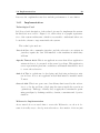
The Sensor Utility Maximization model assumes that the budget is the
demand and that the cost is the utility. Therefore, a solution cannot
give a mission more than its demand. It is a reasonable model where
there is a strong correlation between the utility (and therefore profit) to
the cost.
Prof. Amotz Bar-Noy, City University of New York.
Contents
Abstract
xiii
Introduction
1
1 Sensor Deployment in a Battlefield
3
1.1
1.2
Introduction and Motivations . . . . . . . . . . . . . . . . . . .
3
1.1.1
Context: the ITA project . . . . . . . . . . . . . . . . . .
3
1.1.2
Goal . . . . . . . . . . . . . . . . . . . . . . . . . . . . .
4
1.1.3
Motivations . . . . . . . . . . . . . . . . . . . . . . . . .
5
1.1.4
The virtual environment: “Battlefield 2” . . . . . . . . .
6
Related Work . . . . . . . . . . . . . . . . . . . . . . . . . . . .
8
1.2.1
Previous works on sensors . . . . . . . . . . . . . . . . .
8
1.2.2
The project “Plan and Play” . . . . . . . . . . . . . . .
9
1.2.3
1.3
1.4
1.5
Constraint Satisfaction Problem and
Constraint Programming . . . . . . . . . . . . . . . . . . 11
Concept and Design
. . . . . . . . . . . . . . . . . . . . . . . . 19
1.3.1
System Architecture . . . . . . . . . . . . . . . . . . . . 20
1.3.2
Modeling the Sensor Deployment as a CSP . . . . . . . . 21
1.3.3
Reformulation using the multiple knapsack problem . . . 25
1.3.4
Modeling considerations . . . . . . . . . . . . . . . . . . 34
Implementation and Testing . . . . . . . . . . . . . . . . . . . . 38
1.4.1
Implementation . . . . . . . . . . . . . . . . . . . . . . . 39
1.4.2
Testing and Evaluation . . . . . . . . . . . . . . . . . . . 43
Conclusion and Future works . . . . . . . . . . . . . . . . . . . 45
1.5.1
Conclusion . . . . . . . . . . . . . . . . . . . . . . . . . . 45
vii
viii
CONTENTS
1.5.2
Future works . . . . . . . . . . . . . . . . . . . . . . . . 45
2 Sensor Assignment to Competing Missions
49
2.1
Introduction and Motivations . . . . . . . . . . . . . . . . . . . 49
2.2
Related Work . . . . . . . . . . . . . . . . . . . . . . . . . . . . 51
2.3
Sensor Utility Maximization Problem definition . . . . . . . . . 54
2.4
Centralized solutions . . . . . . . . . . . . . . . . . . . . . . . . 60
2.5
2.6
2.4.1
Integer Linear Programming Solver . . . . . . . . . . . . 60
2.4.2
Greedy Algorithms . . . . . . . . . . . . . . . . . . . . . 61
2.4.3
(2 + )-Approximation Greedy Algorithm Improved . . . 64
Performances . . . . . . . . . . . . . . . . . . . . . . . . . . . . 71
2.5.1
Assumptions . . . . . . . . . . . . . . . . . . . . . . . . . 71
2.5.2
Experimental Setup . . . . . . . . . . . . . . . . . . . . . 73
2.5.3
Simulation Results . . . . . . . . . . . . . . . . . . . . . 73
Conclusion and Future Work . . . . . . . . . . . . . . . . . . . . 77
Conclusion
79
A Sensor Deployment - User Manual
83
A.1 Starting the system . . . . . . . . . . . . . . . . . . . . . . . . . 83
A.2 Using the system . . . . . . . . . . . . . . . . . . . . . . . . . . 84
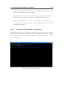
A.2.1 Using the Commander’s Interface . . . . . . . . . . . . . 85
B Sensor Deployment - Maintenance Manual
91
B.1 Installation Instructions . . . . . . . . . . . . . . . . . . . . . . 91
B.2 System Execution . . . . . . . . . . . . . . . . . . . . . . . . . . 93
B.3 Hardware and Software dependencies . . . . . . . . . . . . . . . 94
B.3.1 Hardware dependencies . . . . . . . . . . . . . . . . . . . 94
B.3.2 Software dependencies . . . . . . . . . . . . . . . . . . . 95
B.4 Space and Memory requirements
. . . . . . . . . . . . . . . . . 95
B.5 Source File Description . . . . . . . . . . . . . . . . . . . . . . . 96
B.5.1 Webservice source description . . . . . . . . . . . . . . . 96
B.5.2 Commander Interface source description . . . . . . . . . 98
B.5.3 Battlefield 2 Mod source description
. . . . . . . . . . . 99
CONTENTS
B.6 Compiling and Updating the system . . . . .
B.6.1 Compiling the Webservice . . . . . . .
B.6.2 Compiling the Commander’s Interface
B.6.3 Updating the Battlefield 2 Mod . . . .
B.7 Known Bugs . . . . . . . . . . . . . . . . . . .
B.7.1 Battlefield 2 Mod Bug . . . . . . . . .
B.7.2 Webservice ”Solver” Bug . . . . . . . .
ix
.
.
.
.
.
.
.
.
.
.
.
.
.
.
.
.
.
.
.
.
.
.
.
.
.
.
.
.
.
.
.
.
.
.
.
.
.
.
.
.
.
.
.
.
.
.
.
.
.
.
.
.
.
.
.
.
.
.
.
.
.
.
.
.
.
.
.
.
.
.
100
100
101
101
101
102
102
Acknowledgment
103
Bibliography
107
x
CONTENTS
List of Figures
1.1
A graphic representation of the “Sensor Deployment” problem. .
5
1.2
Map of BF2 on the left, an example of playing on the right. . .
7
1.3
A possible solution to the 8 queens problem. . . . . . . . . . . . 13
1.4
The knapsack problem. . . . . . . . . . . . . . . . . . . . . . . . 15
1.5
Multiple Knapsack Problem . . . . . . . . . . . . . . . . . . . . 17
1.6
System Architecture . . . . . . . . . . . . . . . . . . . . . . . . 20
1.7
Representation of a sensor and a zone in the first model. . . . . 22
1.8
Representation of the Sensor Assignment Problem in the final
model. . . . . . . . . . . . . . . . . . . . . . . . . . . . . . . . . 27
1.9
Analogies between the multiple knapsack and the Sensor Assignment problem. . . . . . . . . . . . . . . . . . . . . . . . . . 28
1.10 Representation of the Sensor Deployment Problem in the final
model. . . . . . . . . . . . . . . . . . . . . . . . . . . . . . . . . 33
1.11 An example of application for the Sensor Deployment Algorithm. 35
1.12 The “Sensor Assignment” model without the heuristic. . . . . . 36
2.1
Modelling Sensor Utility Maximization as a bipartite graph. . . 56
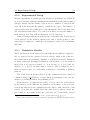
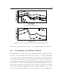
2.2
(200 sensors) Percentage of the optimal fractional solution vs
missions. . . . . . . . . . . . . . . . . . . . . . . . . . . . . . . . 74
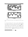
2.3
(500 sensors) Percentage of the optimal fractional solution vs
missions. . . . . . . . . . . . . . . . . . . . . . . . . . . . . . . . 75
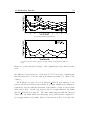
2.4
(1000 sensors) Percentage of the optimal fractional vs missions.
77
A.1 Locating webservice. . . . . . . . . . . . . . . . . . . . . . . . . 85
A.2 Inserting zone side. . . . . . . . . . . . . . . . . . . . . . . . . . 86
xi
xii
LIST OF FIGURES
A.3
A.4
A.5
A.6
A.7
A.8
The side used by the system. . . . . . . . . . . .
Selecting zones. . . . . . . . . . . . . . . . . . .
Creating zones. . . . . . . . . . . . . . . . . . .
Creating Sensors. . . . . . . . . . . . . . . . . .
Solution sent by the webservice. . . . . . . . . .
The message that appears entering a sensor area
. . . . .
. . . . .
. . . . .
. . . . .
. . . . .
in BF2.
.
.
.
.
.
.
.
.
.
.
.
.
.
.
.
.
.
.
.
.
.
.
.
.
87
88
88
89
89
90
Abstract
Questa tesi si colloca nell’ambito della International Technology Alliance (ITA),
progetto che nasce dalla collaborazione tra l’ente di difesa statunitense e inglese. Tale progetto affronta problematiche relative alle operazioni militari
svolte da coalizioni multinazionali e basate su una complessa rete di informazioni, in particolare qui si analizzano reti di sensori.
Quando non è presente una rete di sensori nel campo di battaglia, lo scopo è
quello di dispiegare i sensori in maniera ottima nel campo in modo da soddisfare
i requisiti di informazione di ciascuna missione. L’algoritmo per il posizionamento ottimo dei sensori è basato sul modello di programmazione lineare intera
chiamato “Multiple Knapsack Problem”. Tale algoritmo è stato implementato
come un webservice ed è stato interfacciato con l’ambiente virtuale del gioco
multi-player “Battlefield 2” per effettuare simulazioni realistiche.
Quando è disponibile una rete di sensori già dispiegata sul campo, è tipicamente richiesto il supporto di missioni simultanee in competizione per l’uso
esclusivo dei sensori. Da ciò nasce la necessità di uno schema che assegni i
sensori alle missioni. Qui consideriamo un approccio centralizzato, dove le decisioni vengono prese in un singolo nodo detto “base centrale”. Tale schema è
basato su un modello di programmazione lineare intera chiamato “Generalized
Assignment Problem”.
xiii
xiv
Abstract
Introduction
The aim of this thesis is to give a relevant contribution to the research on sensor
networks, as part of the International Technology Alliance (ITA) project. This
project is funded by the US Army Research Lab and by the UK Ministry of
Defense, and it involves many US and UK universities, together with many big
industries like IBM and Boeing. The aim of the ITA is to face the typical issues
that arise during military operations carried on by multinational coalitions, in
particular this thesis faces the problem of configuring sensor networks on which
military operations have to rely.
The work done in this thesis can be subdivided into two big projects that
are respectively described in Chapter 1 and Chapter 2. These two projects
are very correlated even if it does not seem at a first look. In fact they are
both aiming to configure sensor networks in such a way that the information
requirements of one or more participants in a military operation are satisfied.
Although these two projects were born as solutions to two different problems,
they can be seen as one the extension of the other. In particular the solution
that we developed for the problem faced in Chapter 1 constitutes the foundation on which we constructed the solution for the other problem described in
Chapter 2.
The first project presented in Chapter 1 faces the problem of optimally
deploying sensors in a battlefield, thus creating a sensor network that before
didn’t exists. The sensor network will be deployed with the goal to maximize
the area covered by the sensors, while respecting the information requirements
defined by the commander of a mission. In this project we only consider one
participant at a time in each operation, i.e. each time that a sensor network
1
2
Introduction
must be created there is only one commander who defines the information
requirements from the battlefield. Anyway we also show that our solution can
be easily adapted to deal with multiple missions.
We also describe how we modeled the problem as a Constraint Satisfaction
Problem and in particular as an integer linear programming problem. Indeed,
we extended an existing model, the Multiple Knapsack Problem, to include
necessary informations about the properties of sensors and type of coverage
needed in the battlefield. We present our implemented solution that is a combination of a Constraint Satisfaction Problem Solver and a brand new algorithm.
Since the project aims also to simulate a real world scenario where we can actually deploy the sensors, the solution is implemented as a webservice to allow
independence from the rest of the simulation environment. As environment to
perform our tests we chose the virtual environment of the multi-player game
“Battlefield 2”, and we instrumented it to satisfy our needs. Finally we show
the results of some experiment on the performances of our problem solver, and
we analyze which are the most critical parameters.
The second project is presented in Chapter 2. The assumption here is that
a sensor network is already deployed in a field, and in such a situation it is
usually required to support multiple missions. Since missions might compete
for the exclusive usage of the same sensing resources and since we want to deal
with very large sensor networks, it becomes necessary to develop a sensormission matching scheme.
We formally define the Sensor Utility Maximization problem, an innovative
approach to solve the sensor-mission matching problem. This problem can be
formulated also as an integer linear programming problem, and it is here that
we discover how the Sensor Utility Maximization model can be seen as an
extension of the problem defined in Chapter 1. We decided to consider only
centralized solutions in which the decisions on which sensors are selected and
assigned to missions are made in a single node. We propose greedy algorithms
and we implement a state-of-the-art preexistent algorithm improving its performances. Finally, we also show simulation results comparing the performances
of these proposed solutions.
Chapter 1
Sensor Deployment in a
Battlefield
1.1
Introduction and Motivations
This chapter describe the context of this project giving a brief overview of it,
including also motivations and goals.
1.1.1
Context: the ITA project
This project is part of the ITA project which is an international project led
by IBM1 that addresses researches in the area of network-centric coalition operations. ITA stands for International Technology Alliance in Network and
Information Sciences, and it involves many university in the USA and in the
UK but the main participants are the defense departments of USA and UK
since the results of these researches should be applied to military/rescue missions.
There are four main research areas defined by the alliance: (i) network theory, (ii) security across system of systems, (iii) sensor information processing
and delivery, and finally (iv) distributed coalition planning and decision mak1
website: www.ibm.com
3
4
Introduction and Motivations
ing. The department of Computing Science of the University of Aberdeen2 is
contributing mainly in (iii) and (iv), researching respectively:
1. Knowledge technologies for sensor information processing and delivery
2. Agent technologies for distributed coalition planning and decision making
This project is located inside the research field (1) that is in the area of
sensor researches, in particular its aim is to help the commander of a mission
to define needs of intelligence in certain zones of a map and then to provide the
commander with the optimal deployment of the available sensors inside these
zones. With regards to the ITA project, the most important aspect faced by
this ”Sensor Deployment” project is the scheduling of the capabilities of a
sensor depending on which are the requirements given by the commander. So
for example if there is need of VIDEO information in a certain zone, but the
remaining sensors are all at the same time AUDIO/VIDEO sensors, then it
will be possible to enable only the VIDEO ability of the sensor, in this way the
autonomy of the sensor and also its performance can be increased. Indeed with
only VIDEO enabled the sensor can decide to improve video quality, using the
same energy spent with A/V enabled, or it could decide to maintain the same
VIDEO quality, so that it will spend less energy and in this way the battery
will last longer.
In this Chapter we will describe how we developed an automated reasoning
technique that can generate a ”strategic” deployment of sensors to cover the
requirements of a mission. We will also show how we mathematically modeled
the sensors and of the zones of a map, thing that in the future could be used
as a base to create a sensor and a zone ontology.
1.1.2
Goal
Our project aims, as stated above, to develop an application to help the commander to define his needs of information in certain zones of a map and to give
2
ITA project at Aberdeen: http://www.csd.abdn.ac.uk/research/ita/webpages/projects.html
(last checked 06/05/2007)
1.1 Motivations
5
in output an optimal deployment of the available sensors. Each sensor will be
configured by enabling only certain sensor capabilities depending on the zone
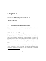
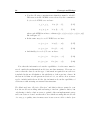
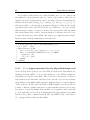
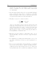
to which their are assigned to. So the problem, which is represented in Figure
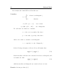
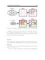
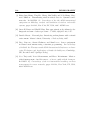
1.1, can be informally defined in this way: Given a set of sensors each one with
its own capabilities and a set of zones, each with its own type of information
required, then the goal is to find an optimal deployment. With ”optimal sensor deployment” we mean that the total area covered by the sensors has to be
maximized, anyway we will see later that the concept ”optimal” can be very
flexible in our solution, since our theoretical approach to the problem is very
flexible too.
Figure 1.1: A graphic representation of the “Sensor Deployment” problem.
The project aims also to simulate a real world scenario, where we can simulate
to deploy the sensors for real. We decided to use a virtual game environment
where it is possible to actually deploy sensors and schedule their capabilities.
Our choice is the virtual world of the PC game ”Battlefield 2”, but our application, as we will see, will be completely independent from this particular
game, so that in the future the virtual environment could be changed or could
be substituted by the real world.
1.1.3
Motivations
The motivations of our project are pretty much the same that lie behind the
ITA project, so overall there is the need to eliminate the pitfalls of compart-
6
Introduction and Motivations
mentalized research in different technical areas3 and, through these researches,
to provide unique capabilities to the US Army and the UK Armed Forces which
could be used either in military or in rescue missions.
Note that in every military/rescue operation the first step is to place some
intelligence in strategic zones (as it is stated in [2]), so that the soldiers know
how they should prepare properly for the current mission. Since the first step
is to deploy sensors and since the result of the mission depends strongly on
the information gathered by the sensors, then it is compulsory to provide a
sensor deployment as good as possible, such that it is able to maximize the
possibilities of success of a mission.
Let’s consider for example the case of a rescue mission in which some citizens
got stuck in a flooded town. The commander will have to decide which are
the zones relevant to the mission, let’s say that these are the most densely
populated areas of the town. Then the commander will decide which type of
information should be required in each area, let’s say AUDIO/VIDEO in some
of them and in others only VIDEO. Our application will have to determine the
optimal positions where to place the sensors and which capabilities of these
sensors have to be enabled. Finally some soldiers could place the sensors, and
the mission could start by using the information gathered by the sensors to
decide which is the first zone to be rescued. So for example in a VIDEO zone
the commander could see through the sensors that it is easier to reach this
zone since it is not already completely flooded.
1.1.4
The virtual environment: “Battlefield 2”
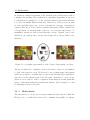
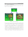
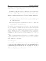
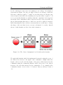
As we said in advance, since we want to simulate a real world scenario, we
used as a virtual environment the world of the PC game ”Battlefield 2”, that
you can see in Figure 1.2. The motivations behind this choice are mainly two:
the tradition of the armed forces to use this kind of games to train soldiers,
3
website: http://domino.research.ibm.com/projects/titans/www titans.nsf/pages/proj.html,
checked on 06/05/2007
1.1 The virtual environment: “Battlefield 2”
7
and the architecture of the game.
Figure 1.2: Map of BF2 on the left, an example of playing on the right.
With regards to the first reason, the US Army uses shooting online games (obviously with a private server) to train soldiers, i.e. they put a bunch of soldiers
in a situation where they have to accomplish a mission and the commander
monitors them by observing the way in which they behave while playing. So
this is not a ”body” or a ”reflex” training but it is a way to improve the strategy applied by each team of soldiers to accomplish a mission. In conclusion
we decided to use ”Battlefield 2” since there is an high probability that soldiers already played a similar game and so if the system developed during this
project should result really interesting with regards to the ITA project, then
it could be also easily tested by the army.
The second motivation that led us to choose ”Battlefield 2” is its architecture.
Indeed it is a shooting online game, that has the typical architecture of an
online game: it has a server and a client. The players will play by starting
the client of the game in their machine and then by connecting to the server
that manages all the interactions with the environment and with other players.
Furthermore it is ”open”, which means that it is easy to gather data and events
from the game, so we can actually know what is happening inside the game.
This can be done by writing some code in Python that we can easily add to
8
Related Work
the game server. In fact this is another important reason that led us to the
choice of using ”Battlefield 2”: it is easy to create ”plug-in’s” for the server
writing our own Python code. Such a ”plug-in” is called ”Mod” (that stands
for ”modified” game) and since there were already many ”Mod” available on
the Internet, likeProject Reality 4 , it was evident that it should have been quite
easy to develop a ”Mod” for this game.
1.2
Related Work
In this Section we give a brief description of the most relevant works produced
on the sensor deployment research area, even if as you will see only one paper
is really interesting for us. We will also introduce a project, developed in the
Computing Science Department of the University of Aberdeen, which is closely
related to this ”Sensor Deployment” project.
1.2.1
Previous works on sensors
The most relevant work for this project is a paper published by IEEE entitled ”Decision-Theoretic Cooperative Sensor Planning”[6]. This paper describes a decision-theoretic approach to cooperative sensor planning between
autonomous vehicles executing a military mission. Simple stated: given a set
of Unmanned Ground Vehicles (UGV) each with sensors installed, they use intelligent cooperative reasoning to select optimal vehicle viewing locations and
to select optimal camera pan and tilt angles throughout the mission. This is
a problem of optimization too, like our ”Sensor Deployment” problem, indeed
the decisions are made in such a way to maximize the value of information
gained by the sensors while maintaining vehicle stealth.
As it can be noticed there are many things in common with our project but
also many different aspects. Anyway the fact that in [6] sensors are mobile
4
which was actually a complete revised version of ”Battlefield 2” (like a new
different game) showing the infinite possibilities of editing this game.
Website:
http://www.realitymod.com/
1.2 The project “Plan and Play”
9
could bring someone to think that this is a big difference with our project,
instead also our approach can be extended to the case where the sensors are
mobile, as we will see in Section 1.3.
The most important thing in common with our project is that they try to compute an optimal location, camera pan and split that can maximize the covered
area for each vehicle, i.e. they are trying to solve a problem that is very similar to our problem. The difference is that they do not have a commander
who specifies which zones have to be covered and which type of information
is required. Instead their commander will only define the value of information
gathered, for example a commander could decide that the value of information
gathered about the kind of enemy forces that is in the area (tank, trucks, etc,)
is the highest valued information, and so the UGV’s will try to find a location
from where they can maximize this type of information.
At the beginning of our project we also thought to use a similar way of giving
a value to the information and then to deploy sensors maximizing this value.
Anyway such a solution turned out to be too complex and it also involved
some aspects that were irrelevant to this project.
Other papers on sensors are available, like in [13] or [9], but none of them
face a problem similar to the optimal sensor deployment. Anyway it is to note
that [9] can be considered very relevant to the branch of the ITA project that
involves sensor networks (which is more or less the same branch to which this
project belongs to).
1.2.2
The project “Plan and Play”
The ”Plan and Play” [11] is the single honours project of Daniele Masato who
developed this project at the Computing Science Department of the University of Aberdeen. ”Plan and Play” is closely related to this project, since our
project uses some concept and technologies developed in Masato’s project.
10
Related Work
Plan and Play finds its collocation in the domain of e-Response, a group of
network technologies designed to support emergency response operations as
humanitarian relief and civilian population control. The project focuses on
human and software agent interactions in a virtual environment where the
collaboration between them is required in order to carry out a plan. So this
project aims to track the progresses achieved in a plan by each player by mapping the plan and its various steps to states and objects within the virtual
universe.
The links between ”Plan and Play” and our project are the architecture of the
system and the virtual environment used. Indeed the architecture of Masato’s
project is based on a central component that is represented by a webservice
written in Java which implements a planner, and as you will see in Section
1.3.1 also the ”Sensor Deployment” project is based on such a webservice.
Another important link between these two projects is the use of the same
virtual environment that is ”Battlefield 2”. In the project ”Plan and Play”,
Masato implemented another webservice (written in Python) inside the game
server5 that exchanges messages with the webservice written in Java but the
”Sensor Deployment” project didn’t need such a complicated ”Mod”6 of the
game, so as we will see in the Section 1.3.1 we only took the same structure of
the ”Mod” (that is a standard for every Mod) and we deleted the webservice
in Python inside the ”Mod” keeping only some useful methods to interact with
the remaining part of the system.
5
The other webservice is the one that implements the planner that is actually completely
independent from the game and also situated outside of it.
6
See Section 1.1.4
1.2 Constraint Satisfaction Problem and
Constraint Programming
1.2.3
11
Constraint Satisfaction Problem and
Constraint Programming
This section describes what is a Constraint Satisfaction Problem (CSP) and
what is Constraint Programming (CP) which are two concepts that we widely
used throughout all this project. We also describe three different Constraint
Satisfaction Problem that are really important with respect to the theoretical
part described in this document.
Definitions: CSP and CP
The ”sensor assignment” problem that we stated above in 1.1.2 can be seen as a
Constraint Satisfaction Problem (CSP) that is a mathematical problem where
one must find values for variables that satisfy a number of constraints. CSPs
are the subject of intense research in both artificial intelligence and operational
research. Many CSPs require a combination of heuristics and combinatorial
search methods to be solved in a reasonable time.
The techniques used to solve a CSP depend on the kind of constraints being
considered. Constraints on a finite domain are often used, to the point that
constraint satisfaction problems are typically identified with problems based
on constraints on a finite domain. Such problems are usually solved via search,
in particular with a form of backtracking or local search. Constraint propagation are other methods used on such problems; most of them are incomplete in
general, that is, they may solve the problem or prove it unsatisfiable, but there
could be cases in which this is not possible. Constraint propagation methods
are also used in conjunction with search methods to make a given problem
simpler to solve.
Constraint programming is the programming paradigm where relations between variables can be stated in the form of constraints. Constraints differ
from the common primitives of other programming languages in that they do
not specify a step or sequence of steps to execute but rather the properties of
a solution to be found.
12
Related Work
The constraints used in constraint programming are of various kinds: those
used in constraint satisfaction problems, those solved by the simplex algorithm,
and others. Constraints are usually embedded within a programming language
or provided via separate software libraries. In our case we will use a Java
software library called “CHOCO”7 that allows us to specify constraints that
will be used by CHOCO itself to solve the “Sensor Deployment” problem with
its own methods used to solve CSP problems.
The eight queens problem
From what stated above, we can easily understand that to solve a CSP it is
enough to specify its constraints with a programming language using some
separate software libraries. So it is clear that the tricky part is not to solve the
problem but to create a mathematical model for the problem, that is to define
variables, the domain of the variables and the constraints for the problem.
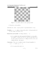
We can understand this by analyzing a CSP problem called “the eight queens
problem”, which is quite related to the ”Sensor Deployment” problem since
it is a placement problem too. In the eight queens problem we have to place
eight chess queens on a 8×8 chessboard in such a way that each queen does
not attack another queen using the standard chess queen’s moves. This problem, as many CSPs, has more than one solution, and you can see one of this
possible solution in Figure 1.3. So it is clear that a solution requires that no
two queens share the same row, column, or diagonal. The eight queens puzzle
is an example of the more general “n queens problem” of placing n queens on
an n × n chessboard.
So now that we informally defined the “n-queens problem”, we can try to
find a mathematical model for this problem. The components of a model are
always three:
1. Variables whose final values have to respect the constraints.
2. Domain of the values that variables can assume.
7
For more information see Section 1.4.
1.2 Constraint Satisfaction Problem and
Constraint Programming
13
Figure 1.3: A possible solution to the 8 queens problem.
3. Constraints on the variables.
And in the case of the “n-queens problem” as presented in the book [1]:
Variables : x1 , . . . , xn . where xi denotes the position of the queen placed in
the ith column of the chess board.
Domain for each variable : the integer values [1, . . . , n] .
• So for example, the solution presented in Figure 1.3 corresponds to
the sequence of values (6,4,7,1,8,2,5,3), since the first queen from
the left is placed in the 6th row counting from the bottom, and
similarly with the other queens.
Constraints : They can be formulated as the following disequalities for
i ∈ [1 . . . n − 1] and j ∈ [i + 1 . . . n]
• No two queens in the same row:
xi 6= xj
(1.1)
14
Related Work
• No two queens in each South-West – North-East diagonal:
xi − xj 6= i − j
(1.2)
• No two queens in each North-West – South-East diagonal:
xi − xj 6= j − i
(1.3)
There is a big difference between an informal description of the problem
and the mathematical model which represents it, indeed we have to reach a
very high level of abstraction.
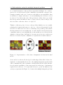
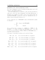
The Knapsack Problem
The knapsack problem is a CSP that derives its name from the maximization
problem of choosing some items that can fit into one bag (of maximum weight)
to be carried on a trip, you can see its graphic representation in Figure 1.4.
An informal description8 of it could be that we are given a set of items, each
with a cost and a value, and a knapsack with a given cost, then we have to
determine which items to insert in the knapsack so that:
• the total cost of the chosen items is less than or equal to
the knapsack’s cost,
• the total value of the chosen items is as large as possible.
In this case it is easier to derive a formal model than in the case of the eight
queens problem, in fact it comes straight forward that the features of the model
are:
Variables : x1 , . . . , xn , where:
8
Here we are actually considering a particular type of knapsack problem called 0-1 knapsack problem, since the items can be chosen (xi = 1) or not chosen (xi = 0). Instead a more
general knapsack problem can also decide to take more than only one instance of the same
object to insert inside the knapsack.
1.2 Constraint Satisfaction Problem and
Constraint Programming
Figure 1.4: The knapsack problem.
xi =


 1


0
if item i is inserted in the knapsack
otherwise
For each item i we define also two constants:
wi := the cost (or weight) of the item i
pi := the value (or profit) of the item i
And one more constant for the knapsack:
c := knapsack’s capacity (or cost)
15
16
Related Work
In the following description of the model we will assume that:
wi ≤ c
(1.4)
so that each item can be (individually) inserted inside the knapsack, and
also that:
n
X
wi ≥ c
(1.5)
i=1
otherwise all the items could be inserted inside the knapsack and this
would be the optimal solution.
Domain: the integer values [0,1] .
Constraints :
n
X
wi · xi ≤ c
(1.6)
i=1
max
n
X
p i · xi
(1.7)
i=1
The first constraint says that the total cost of the chosen items has to be less
than or equal to the knapsack’s cost, and instead the second constraint states
that the total value of the chosen items has to be as large as possible.
The last constraint that maximizes a function is also usually called “Objective Function” and it allows to find the optimal solution between the many
possible solutions to the problem.
The solution of the problem will be a set of values each assigned to a variable:
each variable xi will have a value 0 or 1, where if xi = 1 the item i had been
chosen to be inserted inside the knapsack. This solution will be also optimal,
since the constraint 1.9 states that the total value has to be the highest.
1.2 Constraint Satisfaction Problem and
Constraint Programming
17
It is to note that a problem similar to the “knapsack problem” often appears
in business, cryptography and applied mathematics9 .
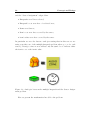
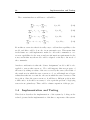
The Multiple Knapsack Problem
The Multiple Knapsack Problem 10 an NP-complete11 Constraint Satisfaction
Problem, i.e. a very hard to solve problem. It is substantially a generalization
of the Knapsack problem explained in the previous Section 1.2.3, indeed the
problem is the same except for the fact that instead of a single knapsack there
are many knapsacks, each with a different cost, where to insert the items. You
can see a graphic representation of the problem in Figure 1.5.
Figure 1.5: Multiple Knapsack Problem
9
See http://en.wikipedia.org/wiki/Knapsack problem , last checked on 09/05/07
Also in this case we are actually considering a particular type of multiple knapsack
problem called 0-1 multiple knapsack problem, since the items can be chosen (xi,j = 1) or
not chosen (xi,j = 0) . Instead in the more general knapsack problem we can also decide to
take more than only one instance of the same item i to insert inside the jth knapsack, so
for example xi,j = 3 means that we are taking three instances of the item i and inserting
them inside the jth knapsack.
11
Also the single knapsack problem is NP-Complete.
10
18
Related Work
Let’s analyze the formal CSP model in this case:
Variables:
xi,j =


 1


if item i is in knapsack j
0
otherwise
∀i ∈ N = {e1 , ..., en }
Set of items
∀j ∈ M = {K1 , ..., Km }
Set of knapsacks
For each item i we define two constants:
wi := the cost (or weight) of the item i
pi := the value (or profit) of the item i
And we also define a constant for each knapsack:
cj := capacity (or cost) of knapsack j
In the following description of the model we will assume that:
max{wi } ≤ max{cj }
i∈N
j∈M
(1.8)
that means that each item can be inserted in at least one knapsack, and
we assume also that:
min{cj } ≥ min{wi }
(1.9)
j∈M
i∈N
which means that each knapsack can contain at least one item.
Domain: the integer values [0,1] .
19
Constraints:
• To ensures that the total cost of items inserted in the jth knapsack
is less than the cost of the jth knapsack:
X
wi · xi,j ≤ cj
∀j ∈ M
(1.10)
i∈N
• To ensures that each item will be inserted in no more than one
knapsack:
X
xi,j ≤ 1
∀i ∈ N
(1.11)
j∈M
• And finally we have the “Objective Function” that states that we
have to maximize the total value of items inserted in each knapsack:
max
XX
pi · xi,j
(1.12)
i∈N j∈M
Note that we could also adapt the “Objective Function” to our needs, by
changing it. Furthermore as we will see in Section 1.3.3, this model will be
the basis over which we will develop the model for our “Sensor Deployment”
problem. Indeed we will take this model and we will expand it with additional
constants and other constraints.
1.3
Concept and Design
This is the most important Section since it describes the solution developed
to solve our problem, but it also gives an overview of the system and an idea
of the first attempt that we did to solve the problem. In particular it is very
interesting how we managed to learn from our mistakes, and how this brought
us to a very good and innovative solution.
20
1.3.1
Concept and Design
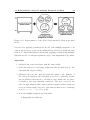
System Architecture
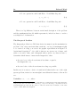
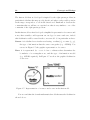
The architecture of the system is an architecture composed by three components, as you can see in figure 1.6.
Figure 1.6: System Architecture
The most important component is the solver, which is an application that
solves the problem of finding an optimal deployment of the sensors inside the
zones of a map given by the commander of a mission. This is implemented
as a webservice and it represents actually the core of the system, since the
remaining two components will interact each other using this webservice as
computation and communication node. It is to note that to implement the
solver we chose the webservice paradigm since in this way the other two components can be easily substituted with different applications if needed. So for
example we could replace the commander’s interface with a more user-friendly
one and the game ”Battlefield 2” with another virtual environment or also
1.3 Modeling the Sensor Deployment as a CSP
21
with the real world.
The second component is the commander’s interface, which allows the commander to choose the zones from a map and to define which type of information
it is required from each of them. At the same time it allows the commander
to insert data about the available sensors, i.e. the number of sensors together
with a set of properties for each one of them. The Commander’s Interface
will send to the solver the information about the sensors and about the zones
selected, so later the solver will solve the problem. It is to note that the solution of the problem remains inside the solver as a static variable, so that at
any time the webservice will contain the current optimal sensor deployment
(if there exists one).
The last component is the mod 12 developed for Battlefield 2 that actually
modifies the behavior of the game server so that when some players connect
to it to play a match, this will ask for the current optimal sensor deployment
stored in the webservice, and then it will create the sensors inside the map.
Anyway we will see in Section 1.4 that the game is quite limited since the only
way in which we can simulate sensors inside the game is creating a sensitive
invisible area that will let us know only what enters and what exits from it.
1.3.2
Modeling the Sensor Deployment as a CSP
Here we describe the real challenge that we faced, that is to create a model
for the “Sensor Deployment” problem. The model for this problem will be
implemented later as a webservice and it will actually constitute the core of
the system.
In this Section we present the first model that we created for the problem,
and as we will notice later we will see that this first model is not appropriate
for this problem. Anyway this model is described in the same way that we will
use to present the final model since we want to describe each step that led us
to develop it.
12
See Section 1.1.4
22
Concept and Design
The first model that we developed is inspired by the eight queens problem, in
particular it idealizes the map as a big chessboard where each possible position
in the map corresponds to a cell in the chessboard. Furthermore between the
constraints that we will use, we can find one that is very similar to one of the
constraint of the eight queens problem.
In this first model we first developed a simplified representation for sensors and
zones, that actually could represent an ontology for sensor and zone, indeed
this idealization will be reused in the correct model. So in particular we have:
Sensor: it is idealized as a circular area having: a radius (ri ), a center (xi , yi ),
the type of information that the sensor can gather (e.g. AUDIO). You
can see in Figure 1.7 the graphic representation of a sensor.
Zone: it is represented by: a set of four coordinates that determines the
boundaries of a rectangular zone, and the type of information needed
(e.g. AUDIO required). In Figure 1.7 we show the graphic idealization
of the zone.
Figure 1.7: Representation of a sensor and a zone in the first model.
Now we can define the formal mathematical model that uses the idealization
showed above:
1.3 Modeling the Sensor Deployment as a CSP
23
Variables: {(x1 , y1 ), . . . , (xn , yn )}
that is a list of (xi , yi ) coordinates of the center of each sensor.
Domain: each (x,y) inside the boundary of the map
Constraints: The constraints can be divided into two types:
1. System Constraints that are actually the constraints proper of the
sensor network, so:
• All the sensors have to be assigned to a different position in the
map:
(xi , yi ) 6= (xj , yj )
∀i, j ∈ {1, . . . , n}, i 6= j
(1.13)
Note that this constraint is really similar to the constraint (1.1)
used in the eight queens model in Section 1.1.
• The area of a sensor must not intersect the area covered by
another sensor, and we implemented this constraint by using
the fact that two circles intersects when the distance between
their centers is less than the sum of their radii:
distance((xi , yi ), (xj , yj )) ≥ |ri +rj |
∀i, j ∈ {1, . . . , n}, i 6= j
(1.14)
2. Commander’s Selection Constraints that are the constraints imposed by the commander when he selects zones in a map and he
decides which type of information it is needed from these zones:
• First of all we divide the sensors in classes considering the type
of information gathered by sensors, so we will have three different classes13 :
AUDIO sensors assume that they are i ∈ {1, . . . , l}
VIDEO sensors assume that they are i ∈ {l + 1, . . . , m}
A/V sensors assume that they are i ∈ {m + 1, . . . , n}
13
Here we consider only three type of information: AUDIO, VIDEO and AUDIO/VIDEO.
Anyway this will be extended in the next Sections.
24
Concept and Design
• Now the following constraint states that there must be only AUDIO sensors in the AUDIO zones selected by the commander.
So for each AUDIO zone we have:
xa ≤ xi ≤ xb
∀i ∈ {1, . . . , l},
(1.15)
ya ≤ yi ≤ yd
∀i ∈ {1, . . . , l},
(1.16)
where each AUDIO zone has coordinates {(xa , ya ), (xb , yb ), (xc , yc ), (xd , yd )}
like in Figure 1.7.
• In the same way, for each VIDEO zone we have:
xa ≤ xi ≤ xb
∀i ∈ {l, . . . , m},
(1.17)
ya ≤ yi ≤ yd
∀i ∈ {l, . . . , m},
(1.18)
• And finally, for each A/V zone we have:
xa ≤ xi ≤ xb
∀i ∈ {m, . . . , n},
(1.19)
ya ≤ yi ≤ yd
∀i ∈ {m, . . . , n},
(1.20)
Note that the information about the capabilities of each sensor must be
stored outside the mathematical model, in some data structure. Viceversa, we
can see that the data about the type of information required from each zone
is included in the model thanks to the subdivision of the zones into classes. In
the last model that we will present in Section 1.3.3, we will see how we managed to include inside the model also the information about the capabilities of
each sensor without using an external data structure.
We didn’t used any “Objective Function” and this is why we wanted to test
how the model was working without having to find an optimal solution, but
only having to find a solution even not optimal. After an implementation step
and some tests we found out that the solver which was using this model was
of a very poor quality, since in many cases it was even not able to find a (non
1.3 Reformulation using the multiple knapsack problem
25
optimal) solution in a reasonable time.
Furthermore we also realized that we were not considering the problem of
scheduling of the capabilities of a multimodal sensor14 . So for example we
were assigning only VIDEO sensors to a VIDEO zone and we were not allowing the case in which an A/V sensor could be assigned to a VIDEO zone
having only the VIDEO capability enabled.
To finish this description of the model we would like to analyze the reasons
why this model did not have good performances. The main reason is that
the domain of this model was too big, in fact taking a closer look at the
domain of the CSPs described in the previous Section 1.2, we can notice that
those domains are really small, sometimes composed by only two elements (e.g.
{0,1}). So it is comprehensible that our model did not work well since our
domain includes each possible position inside a map, that if we have a square
map with a side of 512 meters, the domain will have 512 × 512 = 262144
elements. Here we are considering that the unit of the map is one meter,
and so the smallest distance between two sensors will be one meter. At the
beginning we thought to reduce the domain by taking a unit bigger than one
meter inside the map. So for example by taking 8 meters as a unit in the
map we would have reduced the domain of a factor 82 , indeed the number of
positions allowed in the map now becomes 64 × 64 = 4096. Although in this
way the domain became smaller than before, it was still too big compared to
the domains which ares used in the classic CSPs, and in addition since we used
a bigger unit for the map we lost precision (now the smallest allowed distance
between two sensors is 8 meters). Finally we decided that this was not the
right model and we began to work on a new model.
1.3.3
Reformulation using the multiple knapsack problem
In this section we will describe the final version of the model developed for
the “Sensor Assignment” problem. This model is actually the most important
14
i.e. a sensor with many capabilities (or type of information gathered).
26
Concept and Design
part of this project and as a matter of fact its development took the most part
of the time spent to complete this project.
The intuition behind this model is to think at the “Sensor Deployment”
problem as a “Multiple Knapsack Problem” described in Section 1.2.3, and to
use a similar model for it. This new conception of the problem lead us to divide
the main problem described in Section 1.1.2 into two separate subproblems:
• The “Sensor Assignment” problem that is to assign sensors to zones
considering only the zones selected by the commander and the type of
info required from them.
• The “Sensor Deployment” problem that is for each zone to deploy only
sensors assigned to that particular zone.
This subdivision is very important since it allows also to introduce the scheduling of the capabilities of a multimodal sensor. In fact, just after having found
a solution to the “Sensor Assignment” problem, for a certain sensor with more
than one capability we can choose which capabilities have to be enabled depending on the assigned zone. So for example if an A/V sensor is assigned to
an AUDIO zone, then we will enable only the AUDIO resource of that A/V
sensor.
In the following paragraphs we will describe more in detail the two different
subproblems that will be solved in sequence one after the other and will give
us the optimal sensor deployment.
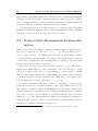
Sensor Assignment
As we stated above, this problem aims to assign sensors considering only the
zones selected by the commander and the type of information that he needs
from these zones, this problem takes also into account the fact that sensors
with many capabilities can be assigned to a zone that does not require that
all the sensor capabilities have to be enabled.
1.3 Reformulation using the multiple knapsack problem
27
So a formal description of the problem, represented in Figure 1.8, could be:
given a set of zones selected by the commander each with its own type of information required, and a set of sensors each with its own capabilities, then
we will have to assign each sensor to a zone maximizing the total area covered
by sensors. Note that at the end of this problem we will not have as a result
the exact positions in which we have to deploy sensors, but we will get only
the zone where each sensor has to be deployed.
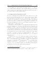
Thanks to this new point of view on the problem definition we are actually
reducing the domain with respect to the one of the model presented in the
Section 1.3.2. Indeed we are no more considering every possible position inside
the map, instead we are now taking into account only the zones selected by the
commander and not even including the positions that are not allowed in the
definition of the problem . In Figure 1.8 we put some red crosses on the zones
that are not selected by the commander to represent the domain reduction.
Figure 1.8: Representation of the Sensor Assignment Problem in the final
model.
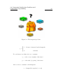
As we said above the model developed for this subproblem called “Sensor Assignment”, is substantially the model of the multiple knapsack extended with
other constraints and other constants to include inside the model the information about the capabilities of the sensors and about the type of information
required from each zone. To begin with let’s try to point out which are the
analogies, represented in Figure 1.9, between the multiple knapsack problem
28
Concept and Design
and the ”Sensor Assignment” subproblem:
• Knapsacks ⇐⇒ Zones selected,
• Knapsack’s cost ⇐⇒ Area of a selected zone,
• Items ⇐⇒ Sensors,
• Item’s cost ⇐⇒ Area covered by the sensor,
• item’s value ⇐⇒ Area covered by the sensor
In particular we note the last two analogies stating that in this case we are
using a specific case of the multiple knapsack problem where pi = wi for each
sensor (or item), so since now we will use only the symbol wi to indicate either
the item’s cost or the item’s value.
Figure 1.9: Analogies between the multiple knapsack and the Sensor Assignment problem.
Here we present the mathematical model for the problem:
1.3 Reformulation using the multiple knapsack problem
29
Variables: We use a two-dimensional variable, to resolve the problem:
xi,j =


 1


0
if sensor i is in zone j
otherwise
∀i ∈ N = {s1 , ..., sn }
∀j ∈ M = {Z1 , ..., Zm }
Set of sensors
Set of zones
And then we use some constant terms for each sensor and for each zone:
tai =


 1


tbi =
0


 1


0
if sensor i has AUDIO
otherwise
if sensor i has VIDEO
otherwise
wi = area covered by sensor i
cj = area of the zone j
Note that an AUDIO/VIDEO sensor will have tai = 1 and tbi = 1.
Below, we also subdivide the set of zones into subsets, each subset is
composed by zones from which the commander requires the same type
of information:
Ma = {Z1 , ..., Zl }, Set of zones from which AUDIO is required.
Mb = {Zl+1 , ..., Zf }, Set of zones from which VIDEO is required.
30
Concept and Design
Ma,b = {Zf +1 , ..., Zm }, Set of zones where both AUDIO and VIDEO
are required.
Domain: the integer values [0,1] .
Constraints:
• The following constraints are the proper constraints of the multiple knapsack problem, like the constraints described in the Section
1.2.3:
X
wi · xi,j ≤ cj
∀j ∈ M
(1.21)
i∈N
X
xi,j ≤ 1
∀i ∈ N
(1.22)
j∈M
• The constraints below were added to respect the commander’s choices,
in terms of type of information needed in each zone. This is one
of the most important part of the model since it extends the basic
model of the multiple knapsack into a more complex one:
The following constraint is to have only sensors with AUDIO enabled in AUDIO zones:
X
i∈N
tai · xi,j =
X
xi,j
∀j ∈ Ma
(1.23)
i∈N
The following constraint is to have only sensors with VIDEO enabled in VIDEO zones:
1.3 Reformulation using the multiple knapsack problem
X
tbi · xi,j =
i∈N
X
∀j ∈ Mb
xi,j
31
(1.24)
i∈N
The following constraint is to have only sensors with A/V enabled
in A/V zones:
X
tai · tbi · xi,j =
i∈N
X
xi,j
∀j ∈ Ma,b
(1.25)
i∈N
• And, as the last part of the extension of the multiple knapsack
model, we add the following constraint to ensure that there is at
least one sensor in each zone:
X
xi,j ≥ 1
∀j ∈ M
(1.26)
i∈N
Objective function: In this case we preferred to treat the objective function
in a separate paragraph, even if it can always be considered a constraint.
We developed two different objective functions and we decided to use the
second one.
• The first possibility for the objective function maximizes the total
area covered by the sensors, considering the zones altogether:
max
XX
wi · xi,j
(1.27)
i∈N j∈M
• Now the second possibility for the objective function, that is the
function that we chose in the implementation, minimizes the number of sensors used and at the same time maximizes the total area
32
Concept and Design
covered by the sensors:
max
XX
i∈N j∈M
wi · xi,j −
XX
xi,j
(1.28)
j∈M i∈N
In the future we could also change this objective function into a more
complex one.
Note again that in the context of this subproblem the coordinates of the
boundaries of each zone do not matter, we will pay attention to them only in
the next subproblem called “Sensor Deployment”.
Furthermore, it is now possible to configure the resources of each multimodal sensor by switching on or off some of these different capabilities. For
example if an AUDIO/VIDEO sensor is assigned to an AUDIO zone, then
we will enable only the AUDIO capability with the purpose of saving battery
power. Battery life is indeed one of the hardest issues to solve when we have to
configure sensor networks, and with this in mind we can state that this model
is quite an important contribution to the researches in sensors networks.
Finally, we would like to point out that this model is an innovative model
since there is no evidence of other researches that applied an extension of the
multiple knapsack model to the field of sensor assignment. This led us also
to write a research paper [12] on this work that will be published in the Proceedings of the Twenty-seventh SGAI International Conference on Innovative
Techniques and Applications of Artificial Intelligence.
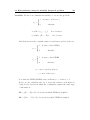
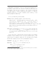
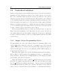
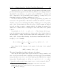
Sensor Deployment
This problem has to be solved separately for each zone, and it can be solved
only after having found a solution for the subproblem called “Sensor Assignment”. A formal description for this second subproblem, represented in Figure
1.10, could be: given a zone and given the subset of sensor assigned to this
zone, then we will have to deploy each sensor inside the zone with the constraint that the areas covered by any two sensors do not overlap.
First of all we have to point out that this is not properly a CSP, but it
1.3 Reformulation using the multiple knapsack problem
33
Figure 1.10: Representation of the Sensor Deployment Problem in the final
model.
is resolved by applying recursively the model of the multiple knapsack, so in
other words we had to create an algorithm that we describe in details into this
Section. To understand what we mean with “applying recursively the multiple
knapsack model” we will just explain the steps of the implemented algorithm.
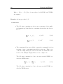
Algorithm:
1. Subdivide the sensors in classes with the same radius.
2. Order the sensors for decreasing radius and take the first class (so the
class with the biggest radius).
3. Subdivide the zone into subzones with side equals to the diameter of
the sensors belonging to the class that we are now considering. In this
way we will have that the area of a subzone can contain only one sensor
belonging to the class currently considered. The area covered by the
sensor is approximated with a square (and not anymore with a circle) and
it is now exactly equal to the area of the subzone that we are considering
now (i.e. cj = wi
∀i ∈ N, ∀j ∈ M ).
4. Solve the multiple knapsack problem with:
• Knapsacks ⇐⇒ Subzones
34
Concept and Design
• Knapsack’s cost ⇐⇒ Area of a subzone
• Items ⇐⇒ Sensors of the first class
• Item’s cost ⇐⇒ Area covered by sensor
• Item’s value ⇐⇒ Area covered by sensor
Note that the last two analogies with the multiple knapsack mean that
also in this case we are using a particular case of it where pi = wi for
each sensor (or item).
5. Deploy sensors inside the subzones as states the solution of the multiple
knapsack problem just resolved. In particular it is clear that all the
sensors of the class will be deployed and none of them will be left out,
since the set of sensors on which we are working is the set of sensors
assigned to this zone from the “Sensor Assignment” model (which will
check that the total area covered by sensors is less than or equal to the
area of the zone).
6. Start from the beginning of the algorithm considering the next class of
sensor and always the same zone, but this time the zone will be subdivided into smaller subzones having side equals to the diameter of the
next class of sensors (which have a smaller radius than the previous
class). Moreover we will have to exclude the subzones that are already
covered by each of the bigger sensors deployed during the previous cycle.
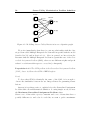
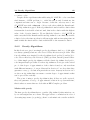
Let’s analyze an example that is also represented in Figure 1.11. If we
have two classes of sensors then the algorithm will cycle twice: the first time it
will assign the sensors that belongs to the class with the biggest radius to the
subzones having as side the diameter of these sensors, the second time it will
exclude the subzones already occupied by the sensors of the first class, and
then it will assign the sensor of the second class to the new smaller subzones.
1.3.4
Modeling considerations
As we already wrote, the first subproblem called “Sensor Assignment” is the
hardest to solve but also the most important. The first subproblem can be
1.3 Modeling considerations
35
Figure 1.11: An example of application for the Sensor Deployment Algorithm.
considered a “global problem” since it involves the whole map. Only if we
have a solution for the first subproblem we can go on to solve the second subproblem that can be considered more a “local problem”, since it involves only
one zone and a subset of sensors each time.
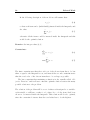
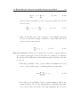
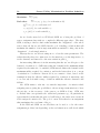
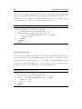
Heuristic
Since both the subproblems are quite hard to solve we used an heuristic, necessary so that the “Sensor Assignment” model described in 1.3.3 could work well.
Heuristic:
“The length of the side of each zone and the length of the radius of each sensor
have to be a power of two.”
If this is violated there could be the case in which the “Sensor Assignment”
36
Concept and Design
model could insert a sensor in a zone putting it out of shape. An example is
represented in Figure 1.12, here we suppose that we are trying to insert the
last sensor, with area equal to 7, inside a zone where there are already some
sensors deployed and where the remaining area is greater than or equal to 7. If
we do not use this heuristic we will have that the constraint 1.21 is respected
and all the other constraints would be respected as well, so the solver will solve
the problem assigning this sensor to that zone even if it couldn’t be inserted.
Indeed inserting the sensor in the zone means that we would have to change
the shape of the area that it can cover (an oval instead of a circle). Instead
the use of this heuristic avoids to have such a situation.
Figure 1.12: The “Sensor Assignment” model without the heuristic.
We apply this heuristic inside the implemented system by using the power of
two that is the nearest to the input of the commander. Simply stated the
length of the zone side and the length of the sensor radius inserted by the
commander using the commander interface will be the power of two that is
nearest to the real value inserted by the commander. So for example if the
commander inserts “sensor radius = 15 meters” then we will use a value of
“16”.
1.3 Modeling considerations
37
Flexibilities of the “Sensor Assignment” model
The “Sensor Assignment” model is very flexible, meaning that it can be well
adapted to many different situations.
The first flexibility that we would like to point out is the fact that it is
really easy to add to the “Sensor Assignment” model many different type of
information. For example if you want to use also sensors that can have the
capability INFRARED, you just need to add some constraints and some constants to the model described in Section 1.3.3.
So let’s consider the case of “INFRARED”, then we will define this constant
for each sensor:
tci =


 1


0
if sensor i has INFRARED
otherwise
Now, we will use these convention: A = AUDIO, V = VIDEO, I = INFRARED; so for example an AUDIO and INFRARED sensor or zone will
be denoted as A/I, instead an AUDIO, VIDEO and INFRARED sensor or
zone will be denoted as A/V/I.
So the types of zones that we can have now become the following:
Ma = {Z1 , ..., Ze }
Set of zones from which “A” is requested.
Mb = {Ze+1 , ..., Zf }
Set of zones from which “V” is requested.
Mc = {Zf +1 , ..., Zg }
Set of zones from which “I” is requested.
Ma,b = {Zf +1 , ..., Zg }
Set of zones from which “A/V” are requested.
Ma,c = {Zg+1 , ..., Zh }
Set of zones from which “A/I” are requested.
Mb,c = {Zh+1 , ..., Zl }
Set of zones from which “V/I” are requested.
Ma,b,c = {Zl+1 , ..., Zm }
Set of zones from which “A/V/I” are requested.
38
Implementation and Testing
The constraints that we will have to add will be:
X
i∈N
X
tci · xi,j =
X
xi,j
tai · tci · xi,j =
X
i∈N
i∈N
X
tbi · tci · xi,j =
X
i∈N
X
i∈N
∀j ∈ Mc
(1.29)
i∈N
xi,j
∀j ∈ Ma,c
(1.30)
xi,j
∀j ∈ Mb,c
(1.31)
i∈N
tai · tbi · tci · xi,j =
X
xi,j
∀j ∈ Ma,b,c
(1.32)
i∈N
From this we can notice that it is really easy to add another capability to the
model, and this could be done also in an automatic way. This means that
in the future we could implement a method to allow the commander to create new capabilities for the sensors and new information requirements for the
zones; and in this way the model could be adapted on the fly to the needs of
the commander.
Another consideration is that the “Sensor Assignment” model could be also
applied to sensors that can move. We could integrate this new property of
the sensor by taking as radius of the area covered by the sensor, the radius of
the actual area in which the sensor can move. So we will simply use a bigger
radius that takes into account also the case in which the sensor can move form
its position. Since the sensor can move, it will have a different position after
a while and so it should be necessary to solve again the problem of deploying
sensors in an optimal way. This could be a future expansion of this project.
1.4
Implementation and Testing
This Section describes the implementation of the system by looking at the
technologies used at the implementation of the three components of the system.
1.4 Implementation
39
Later we also explain the tests done and the performances of our solution.
1.4.1
Implementation
Technologies Used
It follows a brief description of the technologies used to implement the system.
In this Section we refer to Figure 1.3.1, where there is a graphic representation of the system architecture, which is very useful to understand where are
located the software components inside the system.
The technologies used are:
Java 1.6 Since the commander interface and the webservice are written in
java they require the Java VM installed on the machines in which they
will run.
Apache Tomcat 6.0.2 This is an application server that allows application
written in Java to be executed on the server by a client. This application
server represent the platform on which we will install Axis that we need
to create the webservice.
Axis 1.4 This is a platform for developing and deploying webservices written in Java. It is a web application itself that must be installed inside
Tomcat.
choco-1.2.03 This is an open source Java library that is used by the webservice to solve the problem of deploying the sensors inside the zones in an
optimal way. This type of library let you apply the Constraint Programming paradigm, by defining variables, domain, constraints and objective
function.
Webservice Implementation
As we stated above we used Axis to create the Webservice, we chose it because it is really easy to develop new webservices. As a matter of fact we just
40
Implementation and Testing
needed to write your own Java code and insert our packages inside Axis. Then
we created two files of configuration to let Axis know that it had to deploy a
new webservice. Furthermore the installation of Axis, which runs inside the
Apache Tomcat application server, is quite easy to accomplish in a limited
amount of time.
We now give a brief overview of the Java classes that implement the Webservice. This webservice is composed by one package ”deploySensorsService” that
contains a file ”MyService.java” which actually implements the webservice, and
a subpackage ”deploySensorsService.solver” that contains all the classes which
implement the CSP solver using the CHOCO library.
• Let’s consider the package ”deploySensorsService”:
MyService.java This class implements the webservice: the method
”computeDeployment” performs the deployment of the sensors inside the zones, the other methods are used to return to the client
the actual sensor deployment.
The thing that is very important is that once the CSP solver has
solved the problem, then the solution will be stored inside the webservice. So when the BF2 server will ask for the current optimal
deployment, the webservice will return the value of the “static”
variables which contains the data about the optimal deployment.
• Let’s now consider the subpackage ”deploySensorsService.solver”, where
the class that actually solve the problem is ”DeploySensors.java” which
uses ”ZoneDeploy.java” as an auxiliary class. The other classes are data
structures and auxiliary methods used by these two main classes:
DeploySensors.java This class solves in sequence, before the Sensor
Assignment problem (Section 1.3.3) and then the Sensor Deployment problem (Section 1.3.3). This last subproblem is solved using
the class ”ZoneDeploy”.
1.4 Implementation
41
“DeploySensors.java” reflects the global structure of the main problem that is divided into two subproblems: the Sensor Assignment
and then the Sensor Deployment problem. The implementation of
the model is the direct translation of it into CHOCO constraint
language, and because of this also the implementation benefits of
the flexibilities described in Section 1.3.4.
ZoneDeploy.java This class solves the “Sensor Deployment” problem
for each zone considering only the sensors assigned to the zone. This
problem is solved by applying the algorithm described in Section
1.3.3.
Sensor.java This is a data structure that represents the sensor and its
properties. It could be considered as a primitive ontology for the
object Sensor.
CoveredArea.java This is a data structure that represents the zone
selected by the commander and the information that is required
from it. Also this could be considered as a primitive ontology for
the object Zone.
SubArea.java This class represents a subzone created by the division
of a zone into smaller zones, this class is used in the algorithm that
solves the “Sensor Deployment” problem.
Commander’s Interface Implementation
The commander’s interface is actually a command line interface written in
Java, and it sends parameters to the webservice via SOAP messages using particular Java libraries provided by Axis. The commander interface is composed
by one package ”deploySensorsClient” which contains a file “MyClient.java”
and a subpackage “deploySensorsClient.structures”. The first is the main class
of the application and it implements the command-line interface, the second
contains all the data structures used by the interface to perform its tasks (i.e.
the same data structures used by the Webservice solver such as Sensor.java or
CoveredArea.java).
42
Implementation and Testing
• So the package ”deploySensorsClient” contains:
MyClient.java This class implements the Commander’s interface. the
commander can set the parameters of the problem (sensors and
zones) and then these will be sent to the webservice where the
problem will be solved. Finally, the solution will be sent back to the
commander’s interface that will show to the commander the exact
locations in which all sensors will be deployed.
Note that inside this class it is implemented the heuristic that we
described in the Section 1.3.4. In fact when the commander inserts
a length value for the zone side or for a sensor radius, the interface
will automatically compute the power of two that is the nearest to
the number inserted. This will be the real value used to solve the
problem.
“Battlefield 2 Mod” Implementation
As explained in Section 1.1.4, Battlefield 2 allows to develop your own plug-ins
for the server, these plug-ins are called “mod” and they are written in Python.
The real core of the Mod is implemented inside the file ”scoringCommon.py”.
We used also other utility modules that are “Utils.py” and “Defines.py” which
were taken from the mod “PlanAndPlay”.
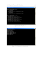
scoringCommon.py This file is the core of the mod: It asks to the webservice for the current sensor deployment (that had been set before by the
commander) and then it creates Sensitive Area inside the map simulating
the behaviour of real sensors.
The issue is that once we created sensors inside the map, we cannot delete
them on the fly while there are still other players inside the map since the game
clients asks for the sensitive area that they have to create inside the local map
only when they join the game. So we had to work out a mechanism that could
delete old sensors and deploy the new sensors belonging to the solution of a
new problem set by the commander:
1.4 Testing and Evaluation
43
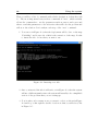
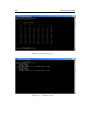
Creating sensors: Each time that the first player join the server loading the
map, the Battlefield 2 server will send a request to the webservice for the
current optimal deployment, and then the Battlefield 2 server will create
the sensors on the map
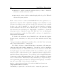
Removing sensors: When the last player disconnects from the current game,
the effect is that the map and all the python code will be reloaded so
that the old sensors created inside the map will be removed. When the
first player will connect to the server and join the game, there will be
again the same sequence of actions described in Creating sensors and
the sensors will be deployed on a clean map.
1.4.2
Testing and Evaluation
Since the most part of the time was spent to develop the model of the problem
and then to implement the whole system, there was not so much time left to
perform tests and evaluate its performances.
Anyway we carried on some interesting tests that highlighted the performances
of the model implementation. Note that we are talking about the performance
of the implementation and not about the performances of the model, since we
know already that the problem is NP-complete, i.e. the solving time will grow
exponentially with the number of parameters used.
During these tests we focused on trying to identify which were the parameters
of the problem that were increasing the solving time the most, and we found
out that these parameters are: the number of sensors and of zones with multiple capabilities, and also the relative dimension of the sensors compared to
the dimensions of the zones15 . Note that the time spent to solve a problem
will not depend from the size of the map thanks to the model, since we are
only considering the number of zones selected by the commander.
15
Meaning that the problem is harder to solve if the sensor area is a lot smaller than the
zone area.
44
Implementation and Testing
We proceed by finding some parameters for the problem that could constitute
a base test case that we could later modify matching our requirements. This
base test takes as parameters 15 sensors of which 5 AUDIO sensors, 5 VIDEO
and 5 A/V; each class of sensor has a different radius that is 64 meters for
AUDIO sensors, 64 for VIDEO and 32 for A/V. Moreover it uses 6 zones all
with the same side of 128 meters16 and with different types of information
needed: two AUDIO zones, two VIDEO and two A/V. It takes more or less
20 seconds to the solver to solve this problem.
Now we consider a variation of this test case decreasing the number of A/V
sensors, i.e. we will have 10 AUDIO sensors, 3 VIDEO sensors and only 2 A/V
sensors, the solving time is only 1 second, a lot better than the previous time.
Finally we considered another variation by increasing the dimension of the
sensor radii and of the zone sides but keeping the same ratio between them
that was used in the base test case. So we will have 5 AUDIO sensors with 128
meters of radius, 5 VIDEO sensors with radius 128, and 5 A/V with radius 64;
instead the side of each of the 6 zones will be 256 meters. This problem takes
20 seconds to be solved that is exactly the same time of the base test case.
We surmised that if the ratio between the dimensions of the sensors and of
the zones remains the same then the time taken to assign sensors to zones will
be the same.
An important issue rises when there is no solution to the problem and the
solver has to understand it. If the problem is “easy” the time to wait will be
very short and it will answer that there is no feasible solution, but if there are
many sensors with small radius and zones with big side, then it will take a lot
of time, and it could also go on indefinitely trying to find a solution. This is
understandable since we are facing a strongly NP-complete problem.
16
Note that the side is equal to the diameters of the AUDIO and VIDEO sensor so one
of these sensors will fit exactly one zone.
45
1.5
Conclusion and Future works
This Section presents some conclusions to our project, discussing which were
our expectations at the beginning of the project and how things actually went.
We also present possible extensions and improvements to our system as future
work.
1.5.1
Conclusion
At the beginning of this project we were not really concerned about the development of a model but we were more worried about the actual implementation,
in particular about how we could represent sensors in Battlefield 2 and how
to integrate everything inside this virtual environment. At the end, instead, it
turned out that the hardest part of the project was to develop the right model
for the problem that we were facing, and after this step the implementation
was quite straightforward, at least for the solver inside the webservice. In any
case we had to spend much time on the design of the webservice and on the
commander’s interface, instead with regards to Battlefield 2 Mod server, we
have been very lucky since the parallel project “Plan and Play” (introduced in
Section 1.2.2) had worked a lot with Battlefield 2 and so we could re-use some
of the knowledge developed in that project.
In conclusion the goal of the project was successfully met and the model that
we developed for the problem seems to be a real innovation in this field.
1.5.2
Future works
There are many future works that could be done starting from this project, but
always keeping as basis the same model described in this document without
changing it very much, since as we showed it is very flexible.
46
Conclusion and Future works
Improving solver: Relaxed Constraints
As we discussed in Section 1.4.2 the solver could spend a lot of time to find
the solution for a problem with many sensors and zones, or it could go on
indefinitely trying to understand if it exists a solution. To improve the solver
performances, we could apply a technique that uses the same model but relaxes
the constraints defined in the problem.
Objective function improvement
In the future we could also try to develop a better objective function, by considering for each item i : pi 6= wi , that are constants that we met in Section
1.3.3, and so we could maximize the total value of the sensors assigned to the
zones. In this way a new objective function could maximize the total area
covered by sensors, minimize the number of sensors used and at the same time
maximize the value of the sensors chosen.
We could also create many different objective functions and then let the decision of which to use to the commander, depending on the requirements of the
particular mission.
Dealing with multiple mission
An interesting feature of this model is that it can already deal with multiple
missions17 . In fact, for example if there are two different commanders for
two different missions, then they will have the same map and the same set
of sensors available to share between the two missions, but they will mainly
select different zones. It is enough to make a join of the two sets of zones and
to pass them together with the set of common sensor to the problem solver,
and it will solve the problem. Actually there could be the need of some minor
adjustments to the model but it should be really straightforward.
17
Here we assume that missions can use the information coming from a sensor at the
same time. So we don’t have the problem to decide to which mission we have to assign a
particular sensor.
1.5 Future works
47
Integration with “Plan And Play”
This project can be integrated with “Plan and Play” (PnP), described in
Section 1.2.2. In fact PnP, as we stated previously, integrates a planner with
Battlefield 2, and this planner receive in input a plan. To integrate PnP with
this project it is enough to write a plan (for the planner) to realize the optimal
deployment of the sensors by sending soldiers to place sensors in the optimal
locations chosen by the solver. So in this case the planner will have as objective
the optimal deployment and it will say to the soldiers how to reach safely the
optimal locations to place sensors.
48
Conclusion and Future works
Chapter 2
Sensor Assignment to
Competing Missions
2.1
Introduction and Motivations
The sensor-mission matching problem is a very complex problem that arises
often in a military environment, when we have to deal with a sensor network
and multiple competing missions. A sensor network consists of a large number
of sensing devices that are able to gather information about the facts happening
in their surroundings. Usually the network of sensors is already deployed in
the field and it is supposed to satisfy the information requirements of multiple
missions. Missions can be competing for the same network resource, and so we
need to find a schema to match sensor resources to missions. In every scenario
a single sensor will have a different degree of utility for a certain mission, since
it will offer to it different quality/quantity of information depending on some
factors (such as distance from a certain point where the task related to the
mission is located). Missions may have different degree of importance (profit)
and different levels of required utility from the sensor network (demand ).
Usually the demand of utility of each single mission is uncertain, for example because of the unknown conditions on the battlefield (e.g. weather, sensor
network damaged, etc.). A concrete example is given by the case in which a
mission needs some video devices but we don’t know the weather conditions
49
50
Introduction and Motivations
and so the visibility range; in such a case the number of video sensing devices
is variable and this means that its utility demand can be considered variable
in a certain range. So it is reasonable to consider that the demand of each
mission is the maximum quality/quantity of information that can be require
from the sensor network. In this situation it is important to assign to the
mission a subset of sensors that will give to the mission a total utility that
will remain under its demand, since the mission could have a real information
requirement that is much less than the one expressed with the demand of the
mission. This means that it is not allowed to ”waste” even a little part of the
informations that the sensor network can collect. Indeed in a common real
scenario it is not allowed to assign to the mission a number of resources that
will supply the mission with more information quantity or quality than the
one needed as maximum. Therefore in our model we consider the demand of
a mission as a budget of required utility not to be exceeded while deciding the
”best” assignment of sensors.
Now the issue is to choose what is meant by “best assignment of sensors
to missions”. Since a sensor will contribute with a different utility to each
mission, we can state that each sensor will bring a different benefit to each
mission, depending on: the fraction of the mission’s demand that the sensor
will satisfy, and also on the importance of the mission itself. Since the benefit
that each sensor can bring to a mission is strongly correlated to the utility
that the sensor has for the mission, in our model we will try to maximize the
total benefit that an assignment of sensors can bring to all the missions by
encouraging the utility to go where it is most helpful, for this reason we chose
for this model the name ”Sensor Utility Maximization”.
In this Chapter, we define the Sensor Utility Maximization (SUM) problem
and show that it is equivalent to a more general problem called Generalized
Assignment Problem (GAP) that is NP-Complete. This more general problem
is well studied in the literature, and as a matter of fact we implemented an
existent (2 + )-approximation greedy algorithm from [5], improving its performances while saving memory space and computational time. We also tried
to implement new greedy algorithms that in many cases have comparable performances. Furthermore we used a linear programming solver (LP solver) to
51
check if it was possible to obtain a good solution in a reasonable time for the
size of our problem instance.
The rest of this Chapter is organized as follows. Section 2.2 discusses
some related work in sensor assignment problems, emphasizing the differences
and similarities with our approach. In Section 2.3 we formally define the
Sensor Utility Maximization problem and study its computational complexity,
showing that it is equivalent to the GAP. In Section 2.4 we describe how
we solved the problem using an LP solver, and we propose our three greedy
algorithms. We give also a description of how we implemented efficiently the
(2 + )-approximation greedy algorithm described in [5]. In Section 2.5, we
evaluate the performances of the proposed solutions using simulations. Finally,
Section 2.6 concludes the paper and outlines some ideas for future work.
2.2
Related Work
There has been a lot of work recently developed on the sensor-mission assignment problem. For example, [4] approaches the assignment problem using the
notions of utility and cost. Here they try to find a solution that maximizes
the utility while staying under a predefined budget, but they use a cost model
based on energy consumption which is different from our cost model based on
the utility demand of every mission. Another important difference is that in
our work we consider multiple missions with different priorities that could possibly compete for the same subset of sensors, instead in [4] the different tasks
do not have a varying priority, so they are considered to be equally important.
A problem that is strongly correlated to SUM is presented in [3] and [8],
which is called the Semi-Matching with Demands (SMD) problem. It models
the problem of assigning sensors to multiple competing missions as a bipartite
graph where nodes can be sensors or missions. Each mission is associated
with a demand value, that is the utility demand required by the mission to
be satisfied, and a profit value, that represents the importance or priority of
the mission/task; each sensor-mission pair is associated with a utility offer
(possibly 0).
52
Related Work
The similarities with the definition of the SUM problem are evident, indeed
SUM can be modeled too as a bipartite graph that resembles exactly the same
graph described in [3] and in [8]. But there are also many important differences. First of all SUM gives a different meaning to the demand of a certain
mission, i.e. it is intended as an upper bound on the utility requested by a
mission, since the utility demanded by a mission is usually very uncertain, as
we noticed in Section 2.1. Anyway the most important difference with our
work is that in SMD model the goal is a sensor assignment that maximizes
the profits of the satisfied missions, with no credit for partially satisfied missions. Instead SUM goal is to assign sensors to missions in which they are
most useful, without caring about the particular satisfaction of each particular
mission. SUM considers only the “global happiness” of the set of mission and
not of every single mission, in such a way that there is no waste of information
gathered by the network.
In this way we loose the concept of satisfaction of a single mission, since we
do not ensure that the amount of sensor utility assigned to a single mission will
satisfy the mission needs of information, but we are now able to assign sensors
to missions in such a way that each sensor will gather the finest informations
for a certain mission, and even if this will not be enough to satisfy the mission,
in every case this will be an information of great value for the mission. So we
are leaving in the background the exact utility demand of a mission, and giving
more importance to the quality of information acquired by the network. In
other words SUM guarantees a very high global QoI (Quality of Information)
for the entire sensor network.
Another thing to observe is that SMD model gives much more importance
to the profit (or importance) value of every single mission, since it uses this
parameter to decide which are the first missions that have to be satisfied. SUM
instead uses this parameter only to scale the utility that the sensor will bring
to the mission, as we will see in Section 2.3. It is because of this that SUM
model could be chosen, instead of SMD, in cases in which the importance of a
mission is very uncertain. In fact in many real life scenarios we have noticed
that the profit value (i.e. importance) of a single mission is never really known,
to determine it exactly we should have an absolute scale that allows us to ex-
53
press the importance of a mission in comparison with other mission profits.
This works for standard missions - for example in the case of an hostage rescue mission that will probably be more important than a mission to detect a
target - but when we deal with more complex missions this clear classification
becomes more undefined.
SUM can also be viewed as a generalization of a model developed for the
sensor deployment problem, introduced in [12] and also in Chapter 1. The
sensor deployment problem is solved in two steps: first, sensors are assigned
to zones, and finally sensors are deployed inside each zones to which they were
assigned. The first subproblem (described in Section 1.3.3) is modeled as an
extension of the multiple knapsack problem which can be considered the base
for the model presented in this paper.
In the extended multiple knapsack model the sensors have some capabilities associated and they can only be assigned to zones that have a request of
information compatible with the capabilities of the sensor1 . Each sensor is also
associated with a coverage area, and each zone has a certain required area to
be covered. The main constraint in this model is that the total area covered by
the set of sensors assigned to the zone must be less than or equal to the area of
the zone. The goal is an assignment of sensors to zone that maximize the total
area covered by the entire set of sensors. It is clear that SUM can be seen as a
generalization of the extended multiple knapsack model: the coverage area of
a sensor in [12] can be compared to the utility offered by a sensor to a mission
in this model, but with the difference that the utility offered can possibly differ
for every mission.
As we will show in Section 2.3, SUM is equivalent to a more general problem
called Generalized Assignment Problem (GAP), often used to solve resource
allocation problems under budget constraints. There exists a lot of literature about this, in particular in [5] and in [7] the authors propose efficient
1
So for example an AUDIO sensor can only be assigned to a zone that requires AUDIO;
but an AUDIO/VIDEO sensor can be assigned to an AUDIO zone, since it can cover the
need of AUDIO informations.
54
Sensor Utility Maximization Problem definition
approximation algorithms which solve the GAP with a certain approximation
guarantee and in a reasonable computational time2 . In Section 2.4, we will describe our implementation of the algorithm described in [5] that we improved
in terms of effective computational time and memory usage.
It is very important to note that, to the best of our knowledge, this is the
first time that GAP is applied to solve a sensor assignment problem, and more
in general a sensor network resource allocation problem.
2.3
Sensor Utility Maximization Problem definition
SUM can be seen as a complete weighted bipartite graph, in which the vertex sets is composed by sensors S = {S1 , . . . , Sn } and by missions M =
{M1 , . . . , Mm } (see Fig. 2.1). Each mission Mj has a positive-valued demand
dj , which indicates the max utility (or quality of information) that a mission
could require. A mission has also an importance (or profit) pj associated with
it, that represents the mission’s priority.
Each edge (Si , Mj ) is associated with two values (eij , pij ). The first eij
indicates the utility that Si could contribute to Mj if it is chosen to assign
sensor Si to mission Mj . The second parameter pij is the benefit (or profit)
that Si could bring to mission Mj , if this pairing were chosen. The parameter
pij includes in it the concept of demand and of importance of a mission, since
it holds always the following equality: pij = eij /dj × pj .
In other words the benefit that a sensor Si can bring to mission Mj is
given by the fraction of demand that the sensor will satisfy, scaled by the
importance of a mission. This last multiplication for the mission importance
allows us during the assignment to favor high priority missions, for example
if we have to assign a sensor which can contribute with the same fraction of
utility (eij /dj ) to two different missions, then we will assign it to the mission
with the highest profit pj since, as we stated before, the benefit pij contains
the fraction of utility contribution scaled by pj .
2
Usually the computational time is correlated to the approximation degree desired.
55
Our goal is an assignment of sensors to missions that maximizes the total benefit (or profit) of the sensor network by sending the utility where it is
most helpful, so that each sensor is assigned to only one mission, and that the
total utility assigned to a mission remains under its demand3 dj . So using the
parameters defined above, we want to maximize a sum of all the pij of each
sensor Si assigned to mission Mj .
Now we can define the problem formally:
Instance: Given a bipartite graph G = (S, M, M P, E, SP ),
where S = {S1 , . . . , Sn } is the vertex set of sensors, M = {M1 , . . . , Mm }
is the vertex set of missions, M P = {p1 , . . . , pm } is the collection of
mission profits, E = {(eij ) : ∀ edges (Si , Mj )} is the collection of sensormission utility associated with the edges S×M . Finally, SP = {(pij ) : ∀ (Si , Mj )}
is the collection of sensor-mission profits associated with the edges, note
that pij = eij /dj × pj .
Goal: Find a semi-matching F ⊆ S × M (i.e. no two chosen edges share the
P
same sensor ), in which (Si ,Mj )∈F pij is maximized for the entire sets
P
S of sensors and M of missions, and where (Si ,Mj )∈F eij ≤ dj for each
mission Mj .
It is probably easier to understand the problem in its Integer Programming
formulation. In the formulation we use one decision variable called xij , indicating if sensor Si is assigned to mission Mj . For each mission Mj we require
that the sum of utility received by Mj is at maximum the value dj .
Maximize:
Such that:
Pm
j=1
Pm Pn
j=1
Pn
i=1
i=1
pij xij , where pij = eij /dj × pj .
xij eij ≤ dj , for each mission Mj ∈ M ,
xij ≤ 1, for each sensor Si , and
xij ∈ {0, 1}, for each variable xij
3
As we explained above the demand is intended as the max utility required by a mission,
since the effective demand of utility is uncertain.
56
Sensor Utility Maximization Problem definition
Sensors
S1
(e11, p11
(e
12
,p
12
)
Missions
)
M1
(d1, p1)
M2
(d2, p2)
S2
S3
S4
Figure 2.1: Modelling Sensor Utility Maximization as a bipartite graph.
We notice immediately that there is a strong relationship with the classic problem called Multiple Knapsack Problem and in specific with the model
described in [12] and in Section 1.3.3. More in general, we know from the
literature that the Multiple Knapsack Problem is a particular case of the Generalized Assignment Problem (GAP), where we use different weights and profit
values for each item with respect to every bin (or knapsack).
Proposition 2.3.1 The SUM problem is the Generalized Assignment Problem
(GAP), hence it follows that SUM is NP-Complete.
Proof:
To show that SUM is identically the same of the GAP, it is enough to
observe the similarities between the two Integer Linear Programming formulations.
Anyway it is perhaps easier to explain before the Generalized Assignment
Problem with a non mathematical definition. So using simple words, we have
the Maximum Generalized Assignment Problem when:
Given a set of bins with capacity constraint and a set of items that have a
possibly different size and value for each bin, we want to pack a maximum-
57
valued subset of items into the bins4 .
Now it is immediate to understand the following Integer Linear Programming formulation of the GAP. About the notation, we indicate the generic
item with an ”i” where i ∈ I = {1, . . . , n}, and the generic bin with a ”j”
where j ∈ J = {1, . . . , m}; for each bin its capacity is denoted with cj . Finally
the size and the value of each item, with respect to every bin, are respectively:
wij and pij . We will use a decision variable called xij , indicating if item i is
assigned to bin j.
Maximize:
Such that:
Pm
j=1
Pm Pn
j=1
Pn
i=1
i=1
pij xij
xij wij ≤ cj , for each bin j
xij ≤ 1, for each item i
xij ∈ {0, 1}, for each variable xij
Now the SUM can be reduced to the GAP (and viceversa) in a polynomial
time, it is enough only to equalize the name of the parameters of the models
described above: wij = eij , cj = dj and pij = pij . It follows that the GAP and
the SUM are the same problem since one can be reduced to the other with a
simple equality between the parameters of their models.
More precisely SUM is an instance of GAP in which there is a strong
correlation between the value and the size of each item (which are sensors in
SUM). Indeed in the Sensor Utility Maximization model we have that the size
of each item is eij and instead the value is pij = eij /dj × pj , so it is clear that
eij and pij are directly proportional in SUM.
Now since GAP is known to be an NP-Complete problem, and since SUM
and GAP are the same problem, thus it follows that also SUM is NP-Complete.
Comparing the SUM model described above with the Semi-matching with
Demands (SMD) model described in the related works (Section 2.2) we can
observe the strong relation between them. We report here for purpose of
comparison the SMD model:
4
For a deeper discussion on GAP, see [5] and [7].
58
Sensor Utility Maximization Problem definition
Maximize:
Such that:
Pm
j=1
Pm
j=1
Pn
pj y j
i=1
xij eij ≥ dj yj , for each mission Mj
xij ≤ 1, for each sensor Si
xij ∈ {0, 1}, for each variable xij
yj ∈ {0, 1}, for each variable yj
As we clearly stated above SUM and SMD are solving the problem of
sensor assignment but with two completely different approaches. The first,
SUM, is trying to find a solution that maximize the “happiness” of the whole
sensor network; the second, SMD, has the goal of finding a solution that will
maximize the number of most important missions satisfied looking only at the
“happiness” of each single mission.
Anyway the two models are using more or less the same parameters. The
values that they have in common are for the missions pj as the importance, dj
as the demand, and instead for the sensor-mission pairs eij .
An interesting difference is in the meaning that the two models give to the
demand of a mission dj . SMD states that the demand is the minimum utility
required by the mission to be satisfied, SUM instead defines the demand as the
maximum utility required by a mission, and in the latter there is no concept
of satisfaction of a mission. Our model is, as a matter of fact, based on the
assumption that the effective utility required by a mission is uncertain, and
so we can only deal with a range of value in which the effective demand could
fall into.
Also SUM wants to take into account the importance of a mission while
assigning sensors giving the possibility to the most important missions to have
the priority on the resources of the sensors, as SMD is doing. SUM tries
to include this concept inside the additional parameter pij , in particular it
represents the benefit that the sensor Si will bring to the entire sensor network
if it is assigned to mission Mj . The goal of our model is therefore an assignment
that maximizes the total sum of the pij .
Both SUM and SMD are models that can be used to solve the sensor
assignment problem, but depending on the real situation we will decide which
59
is the best model to use.
In conclusion, it is better to use SUM when:
• There is high uncertainty about the effective utility demand of missions
(as we stated in 2.1)
• There is high uncertainty about the effective importance of missions (as
we stated in 2.2)
• All the missions have more or less the same importance (or priority).
Indeed when all the missions have comparable priority, it does not matter
to choose which missions to satisfy as SMD, but instead it really matters
to maximize the utility of the entire sensor network that is what SUM is
doing.
• Another interesting scenario in which SUM could be used instead of SMD
is the case in which there are many sensors which have a utility offer eij
that is very similar to the demand dj of each mission.
Let’s analyze a concrete example: suppose that we are given two missions
respectively with demands d1 = 1 and d2 = 1, and suppose we have a
network composed by two sensors with offered utility {e11 = 0.9, e12 =
0.9} for the first sensor S1 , and {e21 = 0.9, e22 = 0.9} for the second
sensor S2 . In this case SMD will assign S1 and S2 to only one mission,
let’s say M1 , leaving M2 completely unsatisfied; instead SUM will assign
each sensor to a different mission, so let’s say S1 to M1 and S2 to M2 . It is
trivial to understand that the first solution wastes a lot of utility offered
by the sensor network and it leaves uncovered a mission that even if it
wouldn’t be entirely satisfied, it could have been almost satisfied. The
second solution instead does not waste any sensor utility and it makes
both mission almost satisfied, and since the assumption of SUM is that
the utility demand dj is the maximum utility demand that a mission
could require, then it could be the case that the real demand of both
missions is less than 1 and in this way we would have satisfied both
missions.
60
2.4
Centralized solutions
Centralized solutions
In this work we describe only centralized approaches to solve the sensor-mission
matching problem, distributed solutions are possible but are not described
here. In a centralized approach all the decisions are made in a base station
which is a special control node in the network. The negative point compared
to the distributed approach is that a centralized solution needs first to collect
all the information in a single node of the network and this requires an higher
number of exchanged messages to configure the network. Anyway the benefit
to use a centralized approach is that we have a global view of the network and
because of this we can probably find a better solution.
We developed different ways of solving the SUM problem: we used an
Integer Linear Programming Solver (lp-solver), we also created four Greedy
Algorithms inspired by the algorithms contained in [3] and in [8], and finally
we improved the performances of the (2+)-Approximation Greedy Algorithm
conceived in [5].
2.4.1
Integer Linear Programming Solver
We first utilized an open source Integer Linear Programming (ILP) solver
called LP SOLVE to check if for the size of our instance we could obtain an
optimal or at least a good solution in a reasonable time, anyway the expectations from this approach were not very high since SUM is NP-Complete, as
we proved in Proposition 2.3.1.
This ILP-solver applies the well known Branch-and-Bound algorithm to
find a solution to Integer Linear Programming problems, i.e. when there are
integer variables, otherwise it uses an implementation of the simplex algorithm
when dealing only with real variables.
Many expedients were used to push LP SOLVE at the best of its possibilities, like for example presolving the problem. The presolve function is built
into LP SOLVE and it analyzes the instance of the problem before applying
the Branch-and-Bound algorithm. The output of this function is the same instance of the problem but with a reduced number of constraints and variables,
2.4 Greedy Algorithms
61
so easier to solve.
Despite all the expedients taken while using LP SOLVE to solve a medium
sized instance of SUM problem, i.e. with 500 sensors and 50 missions, the
computational time was too high. Because of this the only way was to use
LP SOLVE was with a timeout of 10 seconds, after which the Branch-andBound algorithm is stopped. If the algorithm has found a feasible solution then
it returns the best feasible solution found, that is the solution with the highest
value of the objective function. We modified the behavior of LP SOLVE in
such a way that if the Branch-and-Bound algorithm does not find any feasible
solution before the timeout, then it will run again with an increasing timeout
until it finds the first feasible solution which will be the returned solution.
2.4.2
Greedy Algorithms
In this Section we give four simple greedy algorithms to find a good (thought
not always optimal) solution to the Sensor Utility Maximization problem. This
four algorithms were inspired by the algorithms developed in [3] and in [8] to
solve Sensor-Matching with Demands (SMD) problem, but the general behavior of this simple greedy algorithms recall the classic algorithms developed to
solve knapsack-style problems. For these algorithms we don’t give a theoretical
proof of the degree of approximation of the solution found, we only test them
with different instances of our problem and in Section 2.5 we show that they
guarantee a very good solution in practical test cases. Anyway in Section 2.4.3
we show an algorithm that can ensure a certain degree of approximation that
can be proved theoretically.
The point of using a greedy algorithm is that, if they are well conceived,
they can guarantee a very good approximated solution in a polynomial time,
that is what we want when we deal with an NP-Complete problem.
Mission-side greedy
The first greedy algorithm that we consider (Algorithm 1) takes missions one
by one and assigns sensors to them. The approach is to sort missions in order of
decreasing importance (or profit) pj , then for each mission it sorts the available
62
Centralized solutions
sensors in decreasing order of utility offered to that mission and assigns them
until the total utility cumulated by the mission stays under the demand dj of
the mission. The complexity of this algorithm is O (mn log n), with n sensors
and m missions. For this to be true m must be O (n log n).
Algorithm 1 Mission-side Greedy
1: sort the missions in order of decreasing pj
2: for each mission Mj in sorted order do
3:
sort unused sensors in decreasing order of eij
4:
for each unused sensor Si in sorted order do
5:
if eij + total utility cumulated by Mj ≤ dj then
6:
assign Si to Mj
7:
end if
8:
end for
9: end for
Sensor-side Greedy
The second algorithm (Algorithm 2) is a greedy algorithm from the point of
view of the sensor. The algorithm assigns each sensor to the mission Mj to
which the sensor is most useful, i.e. to the mission that maximizes pij . The
complexity of this algorithm is O (nm log m), where “m log m” is given by the
fact that we have to find the mission Mj that maximizes pij .
Algorithm 2 Sensor-side Greedy
1: M ← {M1 , . . . , Mm }
2: for each sensor Si in arbitrary order do
3:
Mk ← maxargMj ∈M {pij } (where pij = eij /dj × pj )
4:
if eik + total utility cumulated by Mj ≤ dj then
5:
assign Si to Mk
6:
M ← M − {Mk }
7:
end if
8: end for
2.4 Greedy Algorithms
63
Ordered Sensor-side Greedy
This algorithm (Algorithm 3) is an improvement of the previous algorithm,
indeed the main body is exactly the same of the Sensor-side Greedy. The only
difference is that before processing sensors it sorts them in decreasing order
using as parameter the maximum profit offer of each sensor, i.e. max{pij } between all the missions Mj to which the sensor can contribute. The complexity
is still O (nm log m) if n is O (m log m), otherwise it is O (nm log m + n log n).
This happens because now the algorithm is also doing a preprocessing of the
sensors, and the best sorting algorithm has complexity O (n log n).
Algorithm 3 Ordered Sensor-side Greedy
1: sort the sensors in order of decreasing max{pij }
2: M ← {M1 , . . . , Mm }
3: for each sensor Si do
4:
Mk ← maxargMj ∈M {pij } (where pij = eij /dj × pj )
5:
if eik + total utility cumulated by Mj ≤ dj then
6:
assign Si to Mk
7:
M ← M − {Mk }
8:
end if
9: end for
Ratio Sensor-side Greedy
The last simple greedy algorithm is another modification of the Sensor-side
Greedy, and it is called Ratio Sensor-side Greedy (Algorithm 4). It is very
similar to the Ordered Sensor-side Greedy since it orders the sensors before
processing them, but the difference is that the sensor are ordered by decreasing
max{pij /eij }. Simply stated, we try to assign first the sensors that have the
biggest offered profit and the smallest utility offer to the mission. This is
the classic approach of knapsack problems where it is usual to assign first
items that have a high profit value and a small size, so that it is possible
to maximize the total profit value while packing the highest number of items
into the knapsack since we insert small items before.The complexity of this
algorithm is the same of the Ordered Sensor-side Greedy (Algorithm 3).
64
Centralized solutions
As we will see this in Section 2.5 this will turn out to be one of the worst
algorithms for our problem in terms of goodness of the solution. Indeed in our
specific case we are dealing with pij and eij strongly correlated, in particular we
will have the following: max{pij /eij } = max{pj /dj }, since pij = eij /dj ×pj . So
the sensors will be ordered using as parameter max{pj /dj } that doesn’t really
depend from the sensor but only from the set of mission, so we can conclude
that the preprocessing of sensors is useless. We reported here this algorithm
since in the future there could be cases in which we could have the need to use
a profit offer value (pij ) and a utility offer value (eij ) completely uncorrelated.
In this scenario this algorithm may work really well.
Algorithm 4 Ratio Sensor-side Greedy
1: sort the sensors in order of decreasing max{pij /eij }
2: M ← {M1 , . . . , Mm }
3: for each sensor Si do
4:
Mk ← maxargMj ∈M {pij } (where pij = eij /dj × pj )
5:
if eik + total utility cumulated by Mj ≤ dj then
6:
assign Si to Mk
7:
M ← M − {Mk }
8:
end if
9: end for
2.4.3
(2+)-Approximation Greedy Algorithm Improved
As we showed in Proposition 2.3.1 the SUM problem is the Generalized Assignment problem (GAP), so it becomes natural to solve SUM by using the
algorithms developed for the GAP. The Generalized Assignment Problem is
well studied in the literature and there have already been developed many
approximation algorithms which guarantee different degrees of approximation
on the solution. In fact, since the GAP is NP-Complete it is in general impossible to find an optimal solution in a polynomial time, therefore it becomes
necessary to create algorithms that can find a non-optimal solution but still
good enough. Here we show how we implemented the approximation algorithm
described in [5] that, combined with another algorithm in [10], is provably a
(2 + )-Approximation Greedy Algorithm.
2.4 (2 + )-Approximation Greedy Algorithm Improved
65
An algorithm is an α-approximation algorithm if |OP T | ≤ α · |ALG| for
α ≥ 1, where |ALG| is the value of the objective function for the feasible
solution returned by the approximation algorithm, and |OP T | is the value of
the objective function for the optimal solution5 .
(α+1)-Approximation Algorithm for GAP
We chose to implement the algorithm described in [5] since it is one of the
latest work about GAP, and since it is one of the best and easiest to implement approximation algorithm developed for this problem. In the paper [5]
the authors state that using any α-approximation algorithm for the knapsack
problem, it is possible to construct an (α+1)-approximation algorithm for the
Generalized Assignment Problem in a greedy manner, using the concept of
“residual profits” to assign items to bins.
The main idea of the algorithm is to solve many times the knapsack problem
each time identifying one of the bins of the GAP model as a knapsack, and
identifying as items to insert into the knapsack all the items given in input
to the Generalized Assignment Problem. During each iteration, the knapsack
problem will use as absolute size for the items the size that each of them has
for the current bin, and as absolute profit the residual profit. The residual
= pij if
of an item i for the bin j is defined in this way: pRES
profit pRES
i
i
item i is not selected for any other bin, otherwise pRES
= pij − pik if item i is
i
selected for bin k.
Formally we use a vector T to indicate the tentative schedule during the
algorithm, so T [i] = j means that the item i is scheduled to bin j, instead
T [i] = −1 means that item i is not scheduled to any bin. The residual profit
in iteration j is denoted by PjRES [i] and it holds PjRES [i] = pij if item i is not
scheduled to any bin (T [i] = −1) and PjRES [i] = pij − pik if item i is scheduled
on bin k (i.e. T [i] = k). Using the terminology of the SUM model the knapsack
problem that is solved at each round has these parameters:
• each knapsack is a mission Mj
5
It is probably easier to understand the definition of α-approximation algorithm if we
consider α ≤ 1, then we have that the condition is: α · |OP T | ≤ |ALG| ≤ |OP T |.
66
Centralized solutions
• the capacity of the knapsack is the utility demand dj of the mission Mj
• the items to insert into the knapsack at each round are all the sensors
of the network
• the size of each item is the utility offer that each sensor have for the
mission j
• the profit value for each item is the residual profit defined above, which
is a function of the profit offered pij by each sensor to a mission.
The algorithm adapted to the terminology used by SUM is presented in
Algorithm 5.
Algorithm 5 (α+1)-Approximation Algorithm for GAP
1: for each sensor Si do
2:
T [i] = −1
3: end for
4: for each mission Mj do
5:
Call α-Approximation Alg. for Knapsack to find a solution to mission
Mj using the residual profit function PjRES
6:
for each Si scheduled by the α-Approximation Alg. to Mj do
7:
T [i] = j
8:
end for
9: end for
The complexity of the (α+1)-Approximation Algorithm for GAP is in general O (m · f (n) + m · n), where n is the number of sensors, m is the number
of missions and f (n) is the running time of the α-Approximation Algorithm
for the knapsack.
α-Approximation Algorithm for the Knapsack
From what written above it is clear the need of implementing also an efficient
α-Approximation Algorithm for the Knapsack Problem 6 .
6
Given a set of items, each with a size wi and a value pi , and a knapsack with a given
capacity c, we have to determine which items to insert in the knapsack so that the total size
of the chosen items is less than or equal to the knapsack’s capacity while maximizing the
total value of the chosen items.
2.4 (2 + )-Approximation Greedy Algorithm Improved
67
Our choice fell on one of the most famous approximation algorithm for this
problem which first appeared in [10]. This algorithm is a (1+)-approximation
algorithm7 for an arbitrary > 0, and it is also an FPTAS8 i.e. its time and
space complexity grows polynomially with n (number of items) and 1/, in
particular both space and time complexity are O (n/2 ).
The Ibarra and Kim algorithm is a dynamic programming algorithm, and
it is based on the profit values of the items. It defines the elements of a matrix
A with n rows (one for each item) and |ALG| columns9 (one for each possible
value of the objective function). Since the value of |ALG| is unknown (indeed
it is the one that we want to compute with the algorithm), the matrix A is
defined on U column, where U is any upper bound on the value of the optimal
solution.
In particular, for l = 1, . . . , n and v = 1, . . . , U the element A[l, v] represents the minimum capacity required to obtain a value of the objective function
at least equals to v using only the first l items. If it is impossible to get v as
value of the objective function using only the first l items then the rule is to
set A[l, v] = +∞. Formally:
A[l, v] = min{q :
l
X
i=1
pi xi ≥ v,
l
X
wi xi ≤ 1, xi ∈ {0, 1}, i = 1, . . . , l}
i=1
Once defined all the elements of the matrix A, the value of the optimal
solution is:
|ALG| := max{v : A[n, v] ≤ c}
The entire Ibarra-Kim algorithm is shown in Algorithm 6.
Since this FPTAS requires that each profit value is an integer number, and
since we also have that the time complexity depends strongly by the maximum
item profit, then we need to to use scaled integer profits different from original
item profits. Formally stated, we will use p0i = bpi /δc for i = 1, . . . , n , where
δ depends from the required approximation error in the returned solution10 .
7
So if we set α = (1 + ) it can be considered an α-approximation algorithm.
Fully Polynomial Time Approximation Scheme.
9
|ALG| is the value of the objective function for the approximated solution.
10
δ := np̃ , where p̃ = maxi {pi }
8
68
Centralized solutions
Algorithm 6 FPTAS for the knapsack problem
1: for v = 1, . . . , p01 do
2:
A[1, v] := w1
3: end for
4: for v = p01 + 1, . . . , U do
5:
A[1, v] := +∞
6: end for
7: for l = 2, . . . , n do
8:
for v = 1, . . . , p0l do
9:
A[l, v] := min{A[l − 1, v], wl }
10:
end for
11:
for v = p0l + 1, . . . , U do
12:
A[l, v] := min{A[l − 1, v], A[l − 1, v − p0l ] + wl }
13:
end for
14: end for
Finally to find the real value of the objective function we will have to
backtrack which items are chosen to be inserted into the knapsack and then
we will use the not-scaled profits to compute the original value of the objective
function. So it is easy to understand that, as in all the dynamic programming
algorithms, we also need to keep another matrix of pointers, that will allow
us to backtrack the solution, i.e. to understand which items where inserted in
the knapsack. This matrix of pointers will have the same dimensions of the
matrix A used to compute the optimal value of the objective function.
Improvements of GAP and Knapsack algorithms
So finally we combined the GAP and Knapsack algorithms (as explained in
Algorithm 5) to solve the SUM problem, and at the same time we modified
them with three major improvements.
Implementing the two algorithms without any particular expedient, highlighted that there were problems related to the memory usage and also to the
effective time spent to compute the solution.
As a matter of fact the Knapsack algorithm requires a lot of memory since
it generates two matrices (one to compute the objective function and the other
2.4 (2 + )-Approximation Greedy Algorithm Improved
69
to backtrack the solution) of dimension n × U , where both n and U are very
large. The number of items n is the number of sensors that we generate and in
our experiments this is a very large number since we want to be able to deal
with very big sensor networks (thousands of them). Also the upper bound U
is really large since in the classic implementation of the Knapsack algorithm
this upper bound is computed in this way: U := p̃ · n; such an upper bound is
really not good, especially if we give in input to the knapsack algorithm a large
number of items and the knapsack has a very low capacity (that is exactly the
case of the SUM, since missions requires in average a utility that is reached
by assigning three or at most four sensors to the mission). The fact that the
dimensions of the matrices are very large, has also strong consequences on the
effective computational time of the Knapsack algorithm, since it will have to
fill a very big matrix to find the solution.
We solved the problem of memory usage and of computational time using three
expedients that are described in the following paragraphs.
The first expedient is to reduce the number of items n given in input at
each round of the GAP algorithm to the Knapsack subroutine. Indeed we will
delete from the input items the ones that have a zero profit for that specific
bin j, and also the ones that are too big to fit into the bin (i.e. in terms of the
SUM problem eij > dj , and instead in terms of the Knapsack problem wi > c).
In this way we obtain a remarkable reduction of n, that in our specific test
cases will be from thousands to tens of sensors; so the rows of the two matrices
created by the Knapsack subroutine are drastically reduced.
The second expedient was taken to reduce the number of columns of the
matrices used in the Knapsack subroutine, that is U . Our improvement here
can be described in two step:
P
1. We solve the knapsack problem using the FPTAS with U = i pi and
without creating the matrix of pointers. Finally we will find the value of
|ALG| (the optimal value of the objective function), as described above
in Section 2.4.3. This computation will require much less memory space,
since we use a better upper bound and also since we don’t create the
70
Centralized solutions
matrix of pointers.
2. Now we run again the Knapsack subroutine but with U = |ALG| and
this time we generate also the matrix of pointers to keep track of which
items are inserted into the knapsack. So the algorithms will generate
two matrices with the minimum number of columns, thus saving a lot of
memory space.
The first and second expedients improve both memory usage and effective
computational time, since they reduce the dimensions of the matrix that is used
to solve the problem. Simply stated they limit the search space by reducing
the number of possible states.
The third expedient improves the memory usage but not the effective
time spent to compute the solution in the Knapsack subroutine. It consists in
substituting the n × U matrix used to compute the value of the objective function with a 2 × U matrix (but the matrix of pointers remains always a n × U
matrix). This idea derives from the dynamic programming implementation of
the knapsack algorithm (Algorithm 6), that requires only the value contained
in the previous row l − 1 to compute the value of a row l. Making use of this
observation we can generate only a 2 × U matrix, and we can compute the
value of the cells of a row by keeping only the previous row and overwriting
with the new computed values the current row (that possibly contains older
values no more required).
In conclusion the interesting thing is that using the GAP (α+1)-approximation
algorithm to solve the SUM, which calls as a subroutine the Knapsack
α-approximation algorithm described above (where α = 1 + ), produces a
(2 + )-approximation algorithm for the Sensor Utility Maximization problem where > 0 is the max error that we want in the returned solution.
As it is stated in [5] the time complexity of this algorithm will be a function
of the time complexity of the Knapsack α-approximation algorithm used11 , and
where m is the number of missions and n is the
in particular it will be O mn
2
number of sensors.
11
That is O
n
2
, as we already stated.
71
Finally we observe that, in theory, this is the best possible algorithm to
solve SUM, from both the point of view of approximation guarantee and time
complexity.
2.5
Performances
To evaluate the performances of all the different algorithms that we presented
we will use a Java simulator developed in [8]. In the same way we will assume
that all sensors know their geographical locations.
Each mission has a maximum demand (dj ), which is the maximum amount
of sensing resources that a mission might require, and a profit (pj ), which
represent the importance of the mission (the higher the profit the more important). The utility offer (eij ) of a sensor to a mission is a function of the
geographical distance between them: the closer the sensor to the mission, the
higher its utility. The utility is 1 if the sensor and the mission lie at the same
location.
So it follows that, in the same way, the profit offer (pij ) of a sensor to a
mission will be a function of the distance of the sensor from the mission, but
this value will also be scaled by the profit of the mission considered. In fact it
holds that pij = eij /dj · pij .
2.5.1
Assumptions
Here we summarize the assumptions that we considered:
• Nodes are deployed in uniformly random locations in a 400m×400m field.
When nodes are deployed we ensure that the network is connected.
• Missions are created in uniformly random locations in the field.
• A base station is located in the center of the left edge of the battlefield
(that is rectangular).
• Each mission has an exponentially distributed demand dj , so there will
be many missions with low demand and few missions with high demand
72
Performances
but where the average value of the demand is 2. However, we cap the
demand to a maximum of 6 in order to limit the number of missions with
a too high demand.
• Associated with each mission there is also an exponentially distributed
profit pj , and here the average value is 1. As in the case of the utility
demand, this simulates realistic scenarios in which many missions have
a low priority and few missions are really critical missions.
• The utility of a sensor Si to a mission Mj will be:
eij =


1
2 /c
1+Dij
 0
if Dij ≤ SR
otherwise
where Dij is the distance between Si and Mj , and SR is the global
sensing range. This means that when a sensor have the same location of
a mission then the utility offer is equal to 1, and it models realistic signal
attenuation which is relative to the square of the distance from a source.
When the mission is outside of a sensor’s sensing range the utility is 0.
In our experiments c = 60 and SR = 30m.
• Each sensor can only be assigned to a single mission, and so once assigned the full utility of the sensor is allocated to support the mission
requirement.
• For communication, we assume perfect channels with no errors or collisions. Hence each message is only sent once and it is guaranteed to be
delivered.
• We do not care about the number of messages that have to be exchanged
between sensors and base station to apply the algorithms and then to
configure the network. Indeed in this work we are not looking for the
best algorithm in terms of the one with the less communication overhead.
2.5 Experimental Setup
2.5.2
73
Experimental Setup
In these experiments we assume prior knowledge about all missions, and like in
[8] we perform three different experiments in which the field size (400m×400m)
is kept constant, but the density of the nodes (i.e. number of sensors in the
network) in the field and the number of missions are varied. The number of
sensors in the network is different for each experiment: 200 for the first, then
500, and finally 1000 sensors. For each node density, we vary the number of
missions from 10 to 100, with an increment of 10 at each step.
In the following results we show the average of 10 runs for the Total Network
Profit achieved by the solution, which is the sum of all the profits pij that
sensors have for missions to which they are assigned12 . Our goal is to maximize
this value.
2.5.3
Simulation Results
The Total Network Profit achieved by each different algorithm is compared to
the one achieved by the optimal fractional solution, which is the solution to
the relaxed linear programming formulation of SUM. By relaxed formulation
we mean a linear programming formulation of SUM where xij is not anymore
integer but it becomes real valued, i.e. now we have xij ∈ [0, 1] (and not
anymore xij ∈ {0, 1}). In this solution a sensor could be assigned to more
than one mission, since we could assign each fraction of its utility to different
missions.
The Total Network Profit achieved by the optimal fractional solution is
computed using LP SOLVE as a classic linear programming solver and not
anymore as an Integer Linear Programming solver.
In the first set of results (shown in Fig. 2.2), we show the total network
profit achieved by the different algorithms as a percentage of the total network profit achieved by the optimal fractional solution, with a network of 200
sensors. Note that the optimal fractional solution is not always a strict upper bound on our results, in fact the integrality gap 13 between the relaxed
12
P P
In other words it is again the value of the objective function i j pij xij .
13
If the relaxed solution to an Integer Linear Programming is indicated as |LP R| and the
74
Performances
(a) All algorithms (200 sensors)
(b) Ordered Sensor-side and (2+)-approximation algorithms (200 sensors)
Figure 2.2: (200 sensors) Percentage of the optimal fractional solution vs missions.
LP problem and the ILP problem could be very high. With this in mind,
we see in Figure 2.2a that the (2 + )-approximation algorithm, LP SOLV E
and the Ordered Sensor-side approach are the best solutions to this instance
of the SUM. Since we are using a small number of sensors LP SOLV E often
manages to find a really good solution to the problem, but what is relevant
is that both Ordered Sensor-side and (2+)-approximation algorithms have
performances comparable to LP SOLV E. In Fig. 2.2b we consider only the
Ordered Sensor-side and (2+)-approximation algorithm and we notice that
integer solution is |ILP | then: Integrality Gap =
|LP R|
|ILP |
2.5 Simulation Results
75
(a) All algorithms (500 sensors)
(b) Ordered Sensor-side and (2+)-approximation algorithms (500 sensors)
Figure 2.3: (500 sensors) Percentage of the optimal fractional solution vs missions.
the difference between the two solutions is 0.5%-1% in average, which means
that they have more or less the same performances in terms of goodness of the
solution.
From Figure 2.3 and 2.4 we note that LP SOLV E performances (compared to the Ordered Sensor-side and the (2+)-approximation algorithm performances) decrease with the increment of the number of sensors, in fact with
1000 sensors (Fig. 2.4) the gap between the (2+)-approximation algorithm
and LP SOLV E is around 3%. The same thing happens with the Ordered
Sensor-side algorithm which has increasing lower performances compared to
(2+)-approximation algorithm, this is clearly shown in Fig. 2.3b and 2.4b.
76
Performances
Anyway the gap between LP SOLV E and (2+)-approximation algorithm is
greater than the gap between Ordered Sensor-side and (2+)-approximation
algorithm (which is around 1.5%).
Despite the general degrade of the performances of the other approaches
compared to the (2+)-approximation algorithm while increasing the number
of sensors, we observe a general improvement on the percentage of the optimal
fractional solution achieved by all the algorithms. This is shown in Figure 2.4b
where the maximum percentage of the optimal fractional solution achieved by
the (2+)-approximation algorithm is around 98%, while instead with 200
sensors in Fig. 2.2b was around 84%.
Concentrating for example on Figure 2.4a (but we could also look at Fig.
2.2a and fig:500:a) we notice that keeping constant the number of sensors
while increasing the number of missions leads to a global degradation of the
performances. Indeed, the percentage of optimal fractional solution achieved
by the (2+)-approximation algorithm with 10 missions is around 96%, but
instead while dealing with 100 missions the performances decrease to 92%.
In conclusion, we infer from these results that the best algorithm to solve
the SUM with a very good degree of approximation is the (2+)-approximation
algorithm described in Section 2.4.3, thought this is not the best in terms of
effective time spent to compute the solution and also of memory usage (even if
,
we strongly improved both). The time complexity of this algorithm is O mn
so if we require an high precision in the solution found (i.e. a very small )
we will have a very big multiplicative constant (that is 1/2 ), and this is why
other algorithms with a worse time complexity go faster in real case scenarios.
For all these reasons we believe that the Ordered Sensor-side algorithm is
a good compromise between optimality of the solution found and time and
space complexity performances. In fact, we noticed that the effective time
spent by this algorithm is much less than the time of the (2+)-approximation
algorithm, and also that there is not a big use of the memory to compute the
solution.
77
(a) All algorithms (1000 sensors)
(b) Ordered Sensor-side and (2+)-approximation algorithms (1000 sensors)
Figure 2.4: (1000 sensors) Percentage of the optimal fractional vs missions.
2.6
Conclusion and Future Work
In this Chapter, we defined the Sensor Utility Maximization (SUM) problem,
were the goal is to maximize the total network profit, i.e. to find an assignment
of sensors to missions that maximizes the total benefit for the sensor network
by sending the utility where it is most helpful. We described the differences
and similarities with other similar problems in the literature, and in particular
we compared it to the Sensor Matching with Demands (SMD) problem. We
analyzed its complexity, showing that is NP-Complete and that it is equivalent to the Generalized Assignment Problem (GAP). Furthermore we looked
at several centralized algorithms to solve it, applying also some techniques al-
78
Conclusion and Future Work
ready known for the Generalized Assignment Problem. Our simulation results
show that one of our greedy algorithm, called Ordered Sensor-side greedy, has
performances comparable to the state-of-the-art algorithms developed to solve
GAP.
The challenge now could consist in the development of distributed algorithms to solve SUM, and also to compare the performances of these distributed
approaches with the centralized solutions described in this Chapter.
A very interesting future work could be to modify the SUM model to include
also the concept of effective cost of sensors and budget of missions, maybe
creating a new model that could be seen as the fusion between SUM and
SMD.
Finally, in this paper we assumed that sensor utilities to a mission are
additive. This is not always the case for every scenario, so we could find a way
to modify the SUM model with some side constraints in such a way to cover
also the scenarios in which this is not true.
Conclusion
The two projects presented in this thesis can be considered a very relevant
contribution to the branch of the International Technology Alliance project
(ITA) which deals with sensor networks. Both sensor deployment and sensor
assignment problems were modeled with a kind of knapsack-style approach,
which is the most innovative contribution to ITA. In this way we showed that
techniques developed to solve knapsack problems can be applied in this field
to decide how to deploy and configure military sensor networks.
Indeed, in Chapter 1, we subdivided the sensor deployment problem into
two main subproblems: sensor assignment to zones and sensor deployment inside each zone. The first subproblem was modeled as an extension of the multiple knapsack problem, by including some additional information on sensors
and zones inside the model, and it had been solved using a classic Constraint
Satisfaction Problem solver (even if we could have also used an Integer Linear
Programming solver). For the second part, instead, we developed a very simple
algorithm to automatically deploy sensors assigned to a particular zone.
An interesting approach to solve the extended multiple knapsack model
could have been to develop greedy and approximation algorithms, based on
the ones already developed in the literature to solve multiple knapsack style
problems. But as a matter of fact in Chapter 2 we implemented a very famous
approximation algorithm to solve the Generalized Assignment Problem (GAP),
and since multiple knapsack is a particular case of GAP we could have used a
similar approach.
Anyway in our experiments we showed that our solution works quite well
for medium sized instances of the problem, but on the other hand it performs
79
80
Conclusion
very badly for big instances since we are using a common CSP solver. The
issue of the time spent is easily solvable by developing an approximation greedy
algorithm for this problem and using this instead of a CSP solver.
Interesting was also the simulation system architecture that we designed
and implemented. We showed that implementing the problem solver as a
webservice makes the system components very independent, so that they are
completely interchangeable. Furthermore we instrumented the game Battlefield 2, with the aim of using it as a simulation environment in which sensors
are deployed using the output of the problem solver. This kind of gaming
virtual environment is often used by US and UK armies to train their soldiers
to improve mission accomplishing strategies; thus in this way our solver could
be really used in the train stage by the commanders. Finally, thanks to the
system architecture the solver could be used also in real world, by substituting
the game server with a real world central station (where decisions to deploy
real sensors are usually taken).
In Chapter 2 we discussed the problem of the sensor assignment to competing missions. This problem differs from the previous one because we now
have to configure an already deployed sensor network and we are using sensors
of the same type (i.e. no multimodal sensors). The interesting fact is that
also this problem was modeled with a knapsack approach, taking inspiration
from the sensor deployment problem already modeled as an extension of the
multiple knapsack.
We formally proved that the sensor assignment problem is equivalent to the
Generalized Assignment Problem (GAP) which is very well studied in the literature. So instead of using a Constraint Satisfaction Problem solver or an Integer Linear Programming solver to solve it, we focused on the development of
new greedy approximation algorithms based on some already developed GAP
algorithms. In particular we showed that the best solution to this NP-complete
problem is given by a version of the very famous (2+)-approximation algorithm described in [10] which we improved with some expedient. Anyway we
also showed that we developed a new greedy approximation algorithm, called
Ordered Sensor-side greedy, which returns a solution that is almost as good
Conclusion
81
as the one returned by the (2+)-approximation algorithm. Furthermore we
observed that Ordered Sensor-side greedy has a running time and a memory
usage that are often better than the ones of the improved (2+)-approximation
algorithm.
Finally, it is reasonable to think that in the real world these two problems
could arise one after the other. A typical scenario in which this could happen
is when there is no sensor network deployed on the battlefield, and so we have
to deploy sensors by maximizing the coverage area and by satisfying all the
mission information requirements. When the sensor network will be deployed
in the battlefield there could be many missions competing for the same sensor
resource, so in this case we have to solve the problem of assigning sensors to
competing missions. In this scenario the assumption is that all the sensors
are of the same type (i.e. there are no multimodal sensors), since the sensor
assignment model was designed only to deal with such sensors.
In conclusion, we believe that this thesis gives a very useful contribution
to the field of military sensor networks. First of all because this is the first
time that somebody deals with very big sensor networks, but also because of
the new problems defined and the new solutions developed to solve them.
82
Conclusion
Appendix A
Sensor Deployment - User
Manual
This manual documents how to run the system described in Chapter 1 – it
should be helpful to a commander who wants to know which are the best positions where to place sensors, given a set of available sensors and of selected
zones of a map.
Note: This manual assumes that you have already installed the system correctly, if you didn’t please see the Maintenance Manual (Appendix B) and
follow the Installation Instructions.
A.1
Starting the system
There are three main components which require to be executed at the same
time - the webservice, the Battlefield 2 mod server and the Commander’s
Interface.
The webservice can be executed by simply starting the Apache tomcat
service, that under WindowsXP can be done by selecting ”Start→Configure
Tomcat” and then by pushing the ”Start” button. This will automatically
start also the Axis Platform that is located inside Apache Tomcat (after a
proper installation of the system), and so it will also start the webservice
83
84
Using the system
called ”DeploySensorsService”.
The Battlefield 2 mod server can be executed by browsing to the folder
”Battlefield2/ServerConfig” and then executing the file ”bf2server.exe”. Note
that before executing the server, it has to be configured with the correct IP, as
specified in the README file inside the installation folder ”Software/Battlefield
2 Mod”.
The Commander Interface can be simply executed by browsing into its
folder and then by clicking on the file ”ComInterface.bat” if you are in a
WindowsXP environment. If you are not under WindowsXP you have to open
a command prompt, browse to the folder ”CommanderInterface” and then
type:
java -jar ComInterface.jar
Finally all the BF2 players that wants to use this infrastructure can start
their game client modified with the Mod that is supposed to be correctly installed in their machine. To start the game mod installed in a client machine
you just need to browse to the folder of the game ”Battlefield2” and then click
on ”RunBF2Client Debug.bat” or on ”RunBF2Client Release.bat”, depending
if you want to run the game in debug1 or in release2 . Note that before allowing
the first player to connect to the BF2 server you should be sure to have stored
the deployment of the sensors through the Commander Interface.
A.2
Using the system
Let’s take a look at the typical sequence of operations in such a system:
1. Start the webservice, the BF2 mod server and the commander interface.
2. Use the commander interface to create sensors and select zones and then
wait for the answer of the webservice, that will solve the problem (if
1
that means in a window at a lower resolution, with the possibility to see debug/error
messages
2
that means at higher resolution on full screen
A.2 Using the Commander’s Interface
85
there is a solution). At the same time, the WebService will store the
sensor deployment into a static variable.
3. The players can now start their client of the game with the ”Mod” installed and then connect to the server ”PlanAndPlay Test Server”
4. When the first player will connect to the BF2 server, this will ask to
the webservice for the stored sensor deployment (previously set by the
commander interface).
A.2.1
Using the Commander’s Interface
When first executing the commander’s interface you will be prompted to input
the URL of the webservice. If it is in the same machine where you are running
the Commander’s Interface, then you will have only to write “local”, as you
can see in Figure A.1.
Figure A.1: Locating webservice.
86
Using the system
Then you will see a list of commands with a little description of what they will
do. The most important between these commands is “new”, which actually
allows the commander to set the parameters such as sensors and zones and
then to send this parameters to the webservice that will solve the problem and
will store the solution. Let’s analyze each step of the “new” command:
1. You can see in Figure A.2, that the deployment will be done on the map
“PlainMap” and it says also which is the extension of the map. It asks
to insert the side of zone that you want to use.
Figure A.2: Inserting zone side.
2. Once you inserted the side it will write, as in Figure A.3, that the system
will use a different number since the system will actually solve a simplified
version of the problem that you are setting up.
3. Now it asks you how many zones you want to select, as shown in Figure
A.4 and it goes through the details of each zone that you will select, like
in Figure A.5.
A.2 Using the Commander’s Interface
87
Figure A.3: The side used by the system.
4. Then it asks how many sensors are available and it lets you define all the
parameters for each sensor, as shown in Figure A.6.
5. Finally it sends the parameters to the webservice and it waits for the
solution, that will be in the format shown in Figure A.7.
Finally the players can now connect to the Battlefield 2 “Plan And Play
Test Server” and there will have invisible sensors deployed inside the map.
The player knows when he is accessing or exiting a certain sensor area since
on the screen of the player inside the game it will appear a message, as shown
in Figure A.8.
88
Using the system
Figure A.4: Selecting zones.
Figure A.5: Creating zones.
A.2 Using the Commander’s Interface
Figure A.6: Creating Sensors.
Figure A.7: Solution sent by the webservice.
89
90
Using the system
Figure A.8: The message that appears entering a sensor area in BF2.
Appendix B
Sensor Deployment Maintenance Manual
This manual concern the system described in Chapter 1. This brief manual
should be helpful to people who want to install the program, modify the program, extend the program, or be aware of which are the known bugs. In this
document we give also a brief description of each of the source files.
B.1
Installation Instructions
The system is composed by three main component, that are actually three
pieces of software, and each one could be considered as an independent application. Let’s analyze the folder structure in the CD that contains the software
and the source code:
• Software - which contains everything you have to install to run the
system
• src - which contains the source code
The folder Software contains three directories, which reflect the system architecture:
• CommanderInterface - which contains the Interface for the commander
91
92
Installation Instructions
• WebService - which contains the platform where you have to insert the
webservice, and the webservice itself
• Battlefield 2 Mod - which contains the plug-in developed for BF2 and
other needed game patches
Each of these folders contains a README.TXT file that explains how to
install each component. The Commander’s interface can be installed on every
OS since it is written in java and it is a jar file. The webservice is also written
in java so it could be installed on every OS, but the installer for Apache
tomcat included in the CD is only for WindowsXP, so if you want to install
the webservice in a OS that is not WindowsXP you will have to download
the proper version of Apache Tomcat. The BF2 ”mod” (i.e. modified) game
server is exclusively compiled for WindowsXP, so it has to be installed in a
WindowsXP environment.
To check if the webservice is well installed you could start the Apache
Tomcat service, and then you could open a browser and write the following
URL:
”http://localhost:8080/axis” and then click on the link ”List” and verify
that ”DeploySensorsService” is in the list.
Note that it is better to install all the three components on the same machine since this is the default configuration. You can also decide to install the
Commander Interface in a different PC and leave the webservice and the BF2
mod game server on another machine; in this case you will have only to enter
the proper URL of the webservice in the commander interface when it will require the address of the webservice. You could also decide to install all the three
components on three different machines, but to do this you will have to change
the code inside the file ”Battlefield2/mods/PlanAndPlay/scoringCommon.py”
and in particular inside the function ”OnPlayerConnect(player)” and substitute the correct URL of the webservice in the line:
deploy = ServiceProxy("http://localhost:8080/axis/services
/DeploySensorsService?wsdl")
And finally you just need to save the file and to restart the game server.
93
B.2
System Execution
There are three main components which require to be executed at the same
time - the webservice, the Battlefield 2 modified game server and the Commander’s Interface.
The webservice can be executed by simply starting the Apache tomcat
service, that under WindowsXP can be done by selecting ”Start→Configure
Tomcat” and then by pushing the ”Start” button. This will automatically
start also the Axis Platform that is located inside Apache Tomcat (after a
proper installation of the system), and so it will also start the webservice
called ”DeploySensorsService”.
The Battlefield 2 mod game server can be executed by browsing to the
folder ”Battlefield2/ServerConfig” and then executing the file ”bf2server.exe”.
Note that before executing the server, it has to be configured with the correct IP, as specified in the README file inside the installation folder ”Software/Battlefield 2 Mod”.
The Commander Interface can be simply executed by browsing into its
folder and then by clicking on the file ”ComInterface.bat” if you are in a
WindowsXP environment. If you are not under WindowsXP you have to open
a command prompt, browse to the folder ”CommanderInterface” and then
type:
java -jar ComInterface.jar
Finally all the BF2 players that wants to use this infrastructure can start
their game client modified with the Mod that is supposed to be correctly installed in their machine, as specified in the README file in the folder ”Software/Battlefield 2 Mod”. To start the game mod installed in a client machine
you just need to browse to the folder of the game ”Battlefield2” and then click
on ”RunBF2Client Debug.bat” or on ”RunBF2Client Release.bat”, depending
if you want to run the game in debug1 or in release2 . Note that before allowing
the first player to connect to the BF2 server you should be sure to have stored
the deployment of the sensors through the Commander Interface.
1
that means in a window at a lower resolution, with the possibility to see debug/error
messages
2
that means at higher resolution on full screen
94
Hardware and Software dependencies
So, just to understand better the last sentence, let’s see which is the typical
sequence of operations in such a system:
1. Start the webservice, the BF2 mod server and the commander interface.
2. Use the commander interface to create sensors and select zones and then
wait for the answer of the webservice, that will solve the problem (if
there is a solution). At the same time, the WebService will store the
sensor deployment into a static variable.
3. The players can now start their client of the game with the ”Mod” installed and then connect to the server ”PlanAndPlay Test Server” 3 .
4. When the first player will connect to the BF2 server, this will ask to
the webservice for the stored sensor deployment (previously set by the
commander interface).
B.3
Hardware and Software dependencies
This section summarizes the hardware and software dependencies of the entire
system.
B.3.1
Hardware dependencies
There are no particular hardware dependencies, except for Battlefield 2 on the
client side. Indeed it is required a graphic card that has to be in the list of
the graphic cards which are compatible with the game, this list is in the game
requirements. Obviously also all the other requirements of the official game
have to be respected.
Instead for the commander interface, the webservice and the BF2 server
there are no particular hardware requirements.
3
You will have noticed that somewhere we use the name ”PlanAndPlay”, this is because
the ”SensorDeployMod” developed for BF2 has adapted and expanded the code of the Mod
developed by Daniele Masato in the project ”Plan And Play”.
B.3 Software dependencies
B.3.2
95
Software dependencies
Java 1.6 Since the commander interface and the webservice are written in
java they require the Java VM installed on the machines in which they
will run. This is not included inside the CD, but you can download it
from http://java.sun.com.
Apache Tomcat 6.0.2 This is an application server that allows application
written in Java to be executed on the server by a client. This software
is included in the CD.
Axis 1.4 This is a platform for developing and deploying webservices written
in Java. It is itself a web application that has to be installed inside
Tomcat. Also this software is included in the CD
Battlefield 2 and Patches The original Battlefield 2 game is for obvious
reasons not included in the Installation CD. But the other patches that
you will have to install are all attached.
choco-1.2.03 This is a Java library that is used by the webservice to solve
the problem of deploying the sensors inside the zones in an optimal way.
This type of solver is called a CSP4 solver, and so ”choco” is a library to
solve CSP’s. This library is in included in the installation CD.
B.4
Space and Memory requirements
Installing the Battlefield 2 server or client will require 2.3 GB of hard disk
space, and this is the same also for the patches. Anyway if you will install
the server, even if during the installation process they say that it is required
to have 2.3 GB of free space, at the end of the day the space occupied by the
server will be only 530 MB, already including the patches.
With regards to memory requirements, it is not recommended to run the
Battlefield 2 server and the client on the same machine since if there is not
4
Constraint Satisfaction Problem
96
Source File Description
enough memory the performances of the game could be compromised. Another
important thing is that if the problem that the webservice has to solve is very
hard (i.e. if there is a high number of zones and of sensors with different
capabilities), then the webservice could start to use a lot of memory space,
but also of CPU percentage work, to solve the problem.
B.5
Source File Description
As we stated previously, there are three main components and the source
code of them is grouped inside the folder src inside the installation CD. The
directory src contains three subdirectories that reflect the system architecture.
• Webservice - which contains the Java source code of the developed webservice
• CommanderInterface - which contains the Java source code of the Interface for the commander
• Battlefield 2 Mod - which contains the Python source code of the BF2
mod
B.5.1
Webservice source description
The Webservice is composed by one package ”deploySensorsService” which
contains a file ”MyService.java” which implements the webservice, and a subpackage ”deploySensorsService.solver” which contains all the classes that implement the solver of the problem to deploy sensors in the selected zones in an
optimal way.
You will note that inside the folder ”src/webservice” there are also other
folders and installation files that need to be installed before modifying the webservice, since they are the platform that allows the webservice to work. Inside
the folder ”src/ConfigWebService” there are two files called ”deploy.wsdd”
and ”undeploy.wsdd”, the first is the most important since you will have to
use it to deploy the webservice inside the Axis platform (as it is well explained
B.5 Webservice source description
97
in the README file inside that folder), the second can be used in the case
that you have to undeploy the webservice.
• Let’s consider the package ”deploySensorsService”:
MyService.java This class implements the webservice: the method
”computeDeployment” performs the deployment of the sensors inside the zones, the other methods are used to return to the client
the actual sensor deployment.
• Let’s consider the subpackage ”deploySensorsService.solver”, where the
class that actually solve the problem is ”DeploySensors.java” which uses
”ZoneDeploy.java” as an auxiliary class. The other classes are data structures and auxiliary methods used by these two main classes:
DeploySensors.java This class performs the Sensor Assignment and
then the Sensor Deployment of the sensors usign the class ”ZoneDeploy”. This reflects the actual model that divides the main problem
into two subproblems: the Sensor Assignment and then the Sensor
Deployment inside each zone of the sensors assigned to that zone.
ZoneDeploy.java This class solve the Sensor Deployment problem for
each zone considering only the sensors assigned to the zone.
Sensor.java This is a data structure that represents the sensor and its
properties.
CoveredArea.java This is a data structure that represents the zone
selected by the commander and the information that is required
from it.
SubArea.java This class represents a subzone created by division of a
zone, this class is used in the algorithm that implements the Sensor
Deployment problem solver.
MyList.java This class implements a list using an hashtable and it is
used as a utility class by the others.
PairInt.java This class implements an object composed by a pair of
integers
98
Source File Description
Utilities.java This class contains some utility function used by the
classes ”DeploySensors” and ”ZoneDeploy”.
B.5.2
Commander Interface source description
The commander interface is composed by one package ”deploySensorsClient”
which contains a file ”MyClient.java” and a subpackage ”deploySensorsClient.structures”.
The first is the main class of the application and it implements the commandline interface, the second contains all the data structures used by the interface
to perform its tasks (i.e. to send the request to the webservice).
• Let’s consider the package ”deploySensorsClient”:
MyClient.java This class implements the Commander’s interface: it
asks to the webservice for the solution of the problem whose parameters are set by the commander. This class uses the classes in
”deploySensorClient.structures” to set the input parameters (sensors and zones) of the method ”computeDeployment” of the webservice. It uses Axis libraries to communicate with the webservice.
• Let’s consider the subpackage ”deploySensorsClient.structures”, where
there are the data structures used by the commander interface to set the
parameters of the problem. This classes are the same data structures
used by the Webservice solver:
Sensor.java This is a data structure that represents the sensor and its
properties.
CoveredArea.java This is a data structure that represents the zone
selected by the commander and the information that is required
from it.
SubArea.java This class represents a subzone created by division of a
zone.
MyList.java This class implements a list using an hashtable and it is
used as a utility class by the others.
B.5 Battlefield 2 Mod source description
B.5.3
99
Battlefield 2 Mod source description
Battlefield 2 allows to develop your own plug-ins for the server, this plug-ins
are called ”mod” and they are written in Python and inserted into the folder
”mods/[YourModName]”. Each ”mod” has to respect a proper structure, so
it will have to include certain folders and files; in this structure you can insert
your own Python code inside the folder ”mods/[YourModName]/Python/game”
that has to have a fixed structure too, but you can add also your own Python
modules.
So the source of Battlefield 2 Mod is contained in the folder ”src/Battlefield
2 Mod/game” inside the installation CD and it has a fixed structure. The real
core of the Mod is implemented inside the file ”scoringCommon.py” that is entirely written by me, Diego Pizzocaro. We used also other utility modules that
are ”Utils.py” and ”Defines.py” which where taken from the Honors Project
of Daniele Masato, whose name is PlanAndPlay5 .
• Let’s consider the folder ”game” it contains a folder ”gamemodes” and
other files of which the most important is ”scoringCommon.py”:
scoringCommon.py This file is the core of the mod: It asks to the
webservice for the current sensor deployment (that had been set
before by the commander) and then it creates Sensitive Area inside
the map simulating the behaviour of real sensors.
Utils.py it contains some of the utility methods used inside the ”mod”
of BF2. This file is more or less the same of the one written by
Daniele Masato, except that we deleted some functions that were
useless for out own ”mod”.
Defines.py it contains all the constants used inside the ”mod” of BF2.
This file is exactly the same of the one written by Daniele Masato
except that we only use certain constants and not all of them.
5
Indeed we took the same structure of the mod ”PlanAndPlay” developed by Daniele
Masato and, after having removed some part of the mod that we would not have used, we
modified the file ”scoringCommon.py”.
100
Compiling and Updating the system
B.6
Compiling and Updating the system
Let’s explain how to compile/update the different components of the system.
B.6.1
Compiling the Webservice
To begin with, you could use an environment such as eclipse to edit the source
code of the webservice. In this case you could create a new Java project, then
import all the source files respecting the structure in packages (and so you
have to create the packages inside eclipse), and finally you have to add to the
project the needed libraries. For the last step you have to consider that to
compile the project you have to add all the Jar files of Axis (contained in the
folder where you installed Axis, inside the directory ”axis-1 4/lib”) an also the
Jar file ”choco-1.2.03”.
Once you compiled the webservice you have to copy the compiled code inside
Axis and then deploy the service. So the steps are:
1. Copy the folder ”deploySensorsService” (you can leave into it the source
code too) inside the folder where you installed Tomcat and in particular inside the directory ”Tomcat 6.0/webapps/axis/WEB-INF/classes”.
You will have to delete the old folder ”deploySensorsService” contained
inside this directory and then you will have to paste the new one.
2. Start the Apache Tomcat service
3. Open a command prompt and browse to the folder of the project where
you have also the files ”deploy.wsdd” and ”undeploy.wsdd”. Now you
have to undeploy the service with this command:
java -cp %CLASSPATH% org.apache.axis.client.AdminClient undeploy.wsdd
Where it is supposed that you set properly the variable ”%CLASSPATH%” as explained in the README.TXT file inside the folder ”src/WebService”.
B.6 Compiling the Commander’s Interface
101
4. Always using the command prompt, you have now to deploy the service.
And you can do this by writing the following command:
java -cp %CLASSPATH% org.apache.axis.client.AdminClient deploy.wsdd
5. Now restart the Apache Tomcat service and the new modified service
should work.
B.6.2
Compiling the Commander’s Interface
Also in this case you could use Eclipse to edit the source code and compile it.
Like previously explained you have to create a new project in Eclipse respecting
the same package structure, and then to include the necessary libraries. In this
case you have only to include the Jar file ”choco-1.2.03”. Once you compiled
it you can also create a Jar File alway using Eclipse (or Netbeans if you prefer
it).
B.6.3
Updating the Battlefield 2 Mod
As you probably know, Python does not need to be compiled, it is usually an
interpreted language and in this case the server will automatically execute the
Python source code. So once you modified the Python source code contained
in the folder ”src/Battlefield 2 Mod/game” inside the installation CD, you just
need to browse inside the directory where the Mod is actually installed (i.e.
”Battlefield 2/mods/PlanAndPlay/python”), then delete the folder ”game”
and replace it with the new modified one.
B.7
Known Bugs
Even if we tested the system quite a lot, it is likely that there are bugs in the
system, which cannot be resolved because of the limited time assigned to this
project. Here we document some known bugs in our system.
102
B.7.1
Known Bugs
Battlefield 2 Mod Bug
The BF2 server asks to the webservice for the stored deployment only when the
first player connects to the server. In the meanwhile the commander could use
the commander’s interface to set another sensor deployment, but this deployment will not be used until all the players disconnect from the server. When
the last remaining player disconnect from the server, it will reboot itself6 , so
that all the sensors that were created inside the map are deleted. Now when
a player connects again to the server, if it is the first who is going to connect,
the server will ask again for the stored sensor deployment, and finally it will
deploy the sensors inside the map.
The problem is located in the slice of time that the server spend to reboot
itself. During this reboot time, a player can still connect to the server, but it
will not have any deployment available, so in the map there will not be any
sensor. In the future this bug could be resolved by not allowing players to
connect to the server while it is rebooting.
B.7.2
Webservice ”Solver” Bug
The solver inside the webservice cannot always understand when a problem
(whose parameters are set by the commander) has no solution. When the
problem is quite ”easy” it manages to answer that there is no solution, but
when there are too many variables it could go on forever trying to find a
solution. In the future this could be resolved by using a time limit, so that
after this fixed time the solver will stop to look for a solution and will answer
that there is no available solution.
6
In this case with the term ”reboot” we mean the operations that the server carries on
to reload all the Python modules.
Acknowledgment
This research was in part sponsored by the U.S. Army Research Laboratory
and the U.K. Ministry of Defence and was accomplished under Agreement
Number W911NF- 06-3-0001. The views and conclusions contained in this
document are those of the author(s) and should not be interpreted as representing the official policies, either expressedor implied, of the U.S. Army
Research Laboratory, the U.S. Government, the U.K. Ministry of Defence or
the U.K. Government. The U.S. and U.K. Governments are authorized to reproduce and distribute reprints for Government purposes notwithstanding any
copyright notation hereon.
The main thanks goes to Prof. Alun Preece who gave me the opportunity
to contribute with my ideas to the International Technology Alliance project,
helped me to develop my skills and gave me very useful advices. Furthermore
I want to thank him for allowing me to go to New York to the CUNY (City
University of New York) Graduate Center to accomplish the research reported
in this thesis.
A particular thanks goes to Dr. Stuart Chalmers who helped me in the work,
gave me very good advices on how to organize the work. Thanks also for the
very good tips on the gigs in Aberdeen.
I want also to thank Dr. Mario Gomez, Dr. Wamberto Vasconcelos, Dr. Tim
Norman, Geeth de Mel and Chris Burnett for letting me participate in very
interesting meetings and discussions about the ITA project, and for making
the time spent in Aberdeen University very nice during my summer placement.
103
104
Acknowledgment
A particular thanks goes also to Matthew P. Johnson, Hosam Rowaihy and
Prof. Amotz Bar-Noy for the wonderful and very productive period that I
passed in New York during my research visit. For having helped me to develop a very efficient solution to the SUM problem, and for appreciating the
work that is in part presented in this thesis.
A special thanks is for Prof. Luca Schenato for having supported my work
from Italy when I was in Aberdeen and in New York, and for having been so
helpful when I had problems.
Another thanks goes to Dott. Daniele Masato which helped me very much
with the part on Battlefield 2, and with whom I had also very interesting discussions about the remaining part of this thesis. Thanks also for the advices
about the topics which he studied in the Operational Research 2 course in Italy
and that I learned from him, from the lecture notes and from various papers.
I want to thank also all my friends, indeed without them I wouldn’t have
been able to accomplish this work. In particular: Giovanni Gellera, Andrea
Gesmundo, Federico Fiorentin, Kartik G., Melissa Gruenzig, Mar, Estelle and
Florence (i.e. all the italian society) for having stolen my Smarties while I was
writing the first part of my thesis...and also for having donated to me the best
year of my life so far.
I must also thank my lifelong italian friends, because even if I disappeared
for many months during this year, every time that I come back they are always here welcoming me. I should also thank them for many other things but
it would be longer than my thesis. These guys are: Fabio Tonello, Giorgio
Volpe, Paolo Sartore, Alessandro Masutti, Gianni Feltrin, Claudio Cusin, Ivan
Bonanno, Alessandro Scandaletti, Francesca Savioli, Veronica Bassi, Manuela
Mantione, Chiara Zacchettin, Fabio Maran, Alessandra Lazzarotto, Francesco
Casellato, Raffaella Fornasier, Elisabetta Pompilio.
Acknowledgment
105
I want to thank also my acquired uncle Pietro Mior for being so interested
in the work that I have done so far, and also for encouraging me so much in
everything I undertake.
A thanks also to my sister Chiara for having bear me during this five years of
university and for having skyped me so often when I was in Aberdeen and in
New York.
Finally the most important thanks goes to my parents Gabriele and Gina for
having given me an example to emulate that lead me to where I am now, for
having taught me everything I know and for having been so patient during
all my studies. I have to thank them for many other reasons that would take
hundreds of written pages.
106
Acknowledgment
[Translation:]
Devo anche ringraziare i miei amici italiani che mi hanno acompagnato durante
tutta la mia vita. Infatti sebbene sia sparito per molti mesi durante questo ultimo anno, sono sempre pronti a darmi il benvenuto a casa ogni volta che torno.
Dovrei ringraziarli anche per tantissime altre cose, ma richiederebbe piú pagine di
questa tesi. I loro nomi sono: Fabio Tonello, Giorgio Volpe, Paolo Sartore, Alessandro Masutti, Gianni Feltrin, Claudio Cusin, Ivan Bonanno, Alessandro Scandaletti,
Francesca Savioli, Veronica Bassi, Manuela Mantione, Chiara Zacchettin, Fabio
Maran, Alessandra Lazzarotto, Francesco Casellato, Raffaella Fornasier, Elisabetta
Pompilio.
Voglio anche ringraziare il mio zio acquisito Pietro Mior per essere sempre cosı́ interessato al lavoro che faccio, e anche per incoraggiarmi sempre moltissimo in ogni
cosa che intraprendo.
Un grazie va anche a mia sorella Chiara per avermi sopportato durante questi cinque
anni di universitá e per avermi telefonato con skype molto spesso mentre ero ad Aberdeen e a New York.
Infine il ringraziamento piú importante va ai miei genitori Gabriele e Gina per
avermi dato un esempio di vita da emulare che mi ha condotto fino a dove sono
arrivato ora, ma anche per avermi insegnato tutto quello che só e per essere stati
cosi pazienti durante tutto il mio percorso di studi. Devo ringraziarli anche per
moltissime altre ragioni ma questo richiederebbe centinaia di pagine scritte.
Bibliography
[1] K. Apt. Principles of constraint programming, 2003.
[2] US Army. Doctrine for intelligence support to joint operations.
http://www.dtic.mil/doctrine/jel/new pubs/jp2 0.pdf.
In
[3] A. Bar-Noy, T. Brown, M. Johnson, T. LaPorta, O. Liu, and H. Rowaihy.
Assigning sensors to missions with demands. In ALGOSENSORS., 2007.
[4] John Byers and Gabriel Nasser. Utility-based decision-making in wireless
sensor networks. Technical Report 2000-014, 1 2000.
[5] Reuven Cohen, Liran Katzir, and Danny Raz. An efficient approximation
for the generalized assignment problem. Inf. Process. Lett., 100(4):162–
166, 2006.
[6] Diane J. Cook, Piotr Gmytrasiewicz, and Lawrence B. Holder. Decisiontheoretic cooperative sensor planning. IEEE Transactions on Pattern
Analysis and Machine Intelligence, 18(10):1013–1023, 1996.
[7] L. Fleischer, M.X. Goemans, V.S. Mirrokni, and M. Sviridenko. Tight
approximation algorithms for maximum general assignment problems. In
Proceedings of the 17th ACM-SIAM Symposium on Discrete Algorithms,
pages 611–620, Miami, Florida, 2006.
[8] H.Rowaihy, M. Johnson, T. Brown, A. Bar-Noy, and T. La Porta. Sensormission matching: Centralized and distributed approaches. In Proceedings
of the 1st Annual Conference of the ITA, Maryland, Washington, September 2007.
107
108
BIBLIOGRAPHY
[9] Hsing-Jung Huang, Ting-Hao Chang, Shu-Yu Hu, and Polly Huang. Magnetic diffusion: disseminating mission-critical data for dynamic sensor
networks. In MSWiM ’05: Proceedings of the 8th ACM international
symposium on Modeling, analysis and simulation of wireless and mobile
systems, pages 134–141, New York, NY, USA, 2005. ACM Press.
[10] Oscar H. Ibarra and Chul E. Kim. Fast approximation algorithms for the
knapsack and sum of subset problems. J. ACM, 22(4):463–468, 1975.
[11] Daniele Masato. Plan and play: Interfacing an htn planner with a virtual
environment. Master’s thesis, University of Padova, Italy, 2007.
[12] Diego Pizzocaro, Stuart Chalmers, and Alun Preece. Sensor assignment
in virtual environments using constraint programming. In Proceedings
of AI2007, the Twenty-seventh SGAI International Conference on Innovative Techniques and Applications of Artificial Intelligence, Cambridge,
UK, December 2007. Springer-Verlag.
[13] Goce Trajcevski, Peter Scheuermann, and Herve Brönnimann. Missioncritical management of mobile sensors: or, how to guide a flock of sensors.
In DMSN ’04: Proceeedings of the 1st international workshop on Data
management for sensor networks, pages 111–118, New York, NY, USA,
2004. ACM Press.