1
Lucid Synchrone
Release, version 3.0
Tutorial and Reference Manual
Marc Pouzet
April 2006
$Id: manual.tex,v 1.11 2007/01/08 17:58:09 pouzet Exp $
Contents
I
Lucid Synchrone
9
1 An introduction to Lucid Synchrone
1.1 The core language . . . . . . . . . . . . . . . . . . . . . . .
1.1.1 Point-wise Operations . . . . . . . . . . . . . . . . .
1.1.2 Delays . . . . . . . . . . . . . . . . . . . . . . . . . .
1.1.3 Global declarations . . . . . . . . . . . . . . . . . . .
1.1.4 Combinatorial Functions . . . . . . . . . . . . . . . .
1.1.5 Sequential Functions . . . . . . . . . . . . . . . . . .
1.1.6 Anonymous Functions . . . . . . . . . . . . . . . . .
1.1.7 Local definitions and Mutually Recursive Definition
1.1.8 Shared Memory and Initialization . . . . . . . . . .
1.1.9 Causality check . . . . . . . . . . . . . . . . . . . . .
1.1.10 Initialization check . . . . . . . . . . . . . . . . . . .
1.2 Multi-clock systems . . . . . . . . . . . . . . . . . . . . . .
1.2.1 Sampling: the operator when . . . . . . . . . . . . .
1.2.2 Combining Sampled Streams: the operator merge . .
1.2.3 Oversampling . . . . . . . . . . . . . . . . . . . . . .
1.2.4 Clock constraints and error messages . . . . . . . . .
1.2.5 Equality and scope restrictions in the use of clocks .
1.3 Static Values . . . . . . . . . . . . . . . . . . . . . . . . . .
1.4 Data-types, Pattern matching . . . . . . . . . . . . . . . . .
1.4.1 Type definitions . . . . . . . . . . . . . . . . . . . .
1.4.2 Pattern matching . . . . . . . . . . . . . . . . . . . .
1.4.3 Local Definitions . . . . . . . . . . . . . . . . . . . .
1.4.4 Implicit Definition of Shared Variables . . . . . . . .
1.5 Valued Signals . . . . . . . . . . . . . . . . . . . . . . . . .
1.5.1 Signals as Clock Abstraction . . . . . . . . . . . . .
1.5.2 Testing the Presence and Signal Matching . . . . . .
1.6 State Machines . . . . . . . . . . . . . . . . . . . . . . . . .
1.6.1 Strong Preemption . . . . . . . . . . . . . . . . . . .
1.6.2 Weak Preemption . . . . . . . . . . . . . . . . . . .
1.6.3 ABRO and Modular Reseting . . . . . . . . . . . . .
1.6.4 Local Definitions in a State . . . . . . . . . . . . . .
1.6.5 Communication between States and Shared Memory
1.6.6 The Particular Role of the Initial State . . . . . . .
1.6.7 Resume a Local State . . . . . . . . . . . . . . . . .
3
.
.
.
.
.
.
.
.
.
.
.
.
.
.
.
.
.
.
.
.
.
.
.
.
.
.
.
.
.
.
.
.
.
.
.
.
.
.
.
.
.
.
.
.
.
.
.
.
.
.
.
.
.
.
.
.
.
.
.
.
.
.
.
.
.
.
.
.
.
.
.
.
.
.
.
.
.
.
.
.
.
.
.
.
.
.
.
.
.
.
.
.
.
.
.
.
.
.
.
.
.
.
.
.
.
.
.
.
.
.
.
.
.
.
.
.
.
.
.
.
.
.
.
.
.
.
.
.
.
.
.
.
.
.
.
.
.
.
.
.
.
.
.
.
.
.
.
.
.
.
.
.
.
.
.
.
.
.
.
.
.
.
.
.
.
.
.
.
.
.
.
.
.
.
.
.
.
.
.
.
.
.
.
.
.
.
.
.
.
.
.
.
.
.
.
.
.
.
.
.
.
.
.
.
.
.
.
.
.
.
.
.
.
.
.
.
.
.
.
.
.
.
.
.
.
.
.
.
.
.
.
.
.
.
.
.
.
.
.
.
.
.
.
.
.
.
.
.
.
.
.
.
.
.
.
.
.
.
.
.
.
.
.
.
.
.
.
.
.
.
.
.
.
.
.
.
.
.
.
.
.
.
.
.
.
.
.
.
.
.
.
.
.
.
.
.
.
.
.
.
.
.
.
.
.
.
.
.
.
.
.
.
.
.
.
.
.
.
.
.
.
.
.
.
.
.
.
.
.
.
.
.
.
.
.
.
.
.
.
.
11
11
11
12
12
13
14
16
16
17
18
19
19
19
21
22
25
26
27
28
28
28
31
31
32
32
32
34
35
35
36
37
39
39
41
1.7
1.8
Parameterized State Machines . . . . . . . . .
State Machines and Signals . . . . . . . . . .
1.8.1 Pattern Matching over Signals . . . .
1.8.2 The derived operator await/do . . . .
1.9 Alternative Syntax for Control Structures . .
1.10 Higher-order Reactive Features . . . . . . . .
1.10.1 Composing Functions . . . . . . . . .
1.10.2 Combinators . . . . . . . . . . . . . .
1.10.3 Streams of Functions and Functions of
1.10.4 Instantiating Streams of Functions . .
1.11 Non reactive higher-order features . . . . . .
2 Complete Examples
2.1 The Inverted Pendulum . .
2.2 The Heater . . . . . . . . .
2.3 The Coffee Machine . . . .
2.4 The Recursive Wired Buffer
II
.
.
.
.
.
.
.
.
.
.
.
.
.
.
.
.
.
.
.
.
.
.
.
.
.
.
.
.
.
.
.
.
.
.
.
.
.
.
.
.
. . . . .
. . . . .
. . . . .
. . . . .
. . . . .
. . . . .
. . . . .
. . . . .
Streams
. . . . .
. . . . .
.
.
.
.
.
.
.
.
.
.
.
.
.
.
.
.
.
.
.
.
.
.
.
.
.
.
.
.
.
.
.
.
.
.
.
.
.
.
.
.
.
.
.
.
.
.
.
.
.
.
.
.
.
.
.
.
.
.
.
.
.
.
.
.
.
.
.
.
.
.
.
.
.
.
.
.
.
.
.
.
.
.
.
.
.
.
.
.
.
.
.
.
.
.
.
.
.
.
.
.
.
.
.
.
.
.
.
.
.
.
.
.
.
.
.
.
.
.
.
.
.
.
.
.
.
.
.
.
.
.
.
.
.
.
.
.
.
.
.
.
.
.
.
.
.
.
.
.
.
.
.
.
.
.
.
.
.
.
.
.
.
.
.
.
.
.
.
.
.
.
.
.
.
.
.
.
.
.
.
.
.
.
.
.
.
.
.
.
.
.
.
.
.
.
.
.
.
.
.
.
.
.
.
.
.
.
.
.
.
.
.
41
43
43
45
46
47
47
49
49
49
50
.
.
.
.
52
52
54
57
60
Reference manual
3 The language
3.1 Lexical conventions . . . . . . . . . . . . . . . .
3.2 Values . . . . . . . . . . . . . . . . . . . . . . .
3.2.1 Basic values . . . . . . . . . . . . . . . .
3.2.2 Tuples, records, sum types . . . . . . . .
3.3 Global names . . . . . . . . . . . . . . . . . . .
3.3.1 Naming values . . . . . . . . . . . . . .
3.3.2 Referring to named values . . . . . . . .
3.4 Types . . . . . . . . . . . . . . . . . . . . . . .
3.5 Clocks . . . . . . . . . . . . . . . . . . . . . . .
3.6 Constants . . . . . . . . . . . . . . . . . . . . .
3.7 Patterns . . . . . . . . . . . . . . . . . . . . . .
3.8 Signal Patterns . . . . . . . . . . . . . . . . . .
3.9 Expressions . . . . . . . . . . . . . . . . . . . .
3.9.1 Simple expressions . . . . . . . . . . . .
3.9.2 Operators . . . . . . . . . . . . . . . . .
3.9.3 Control Structures . . . . . . . . . . . .
3.10 Definitions . . . . . . . . . . . . . . . . . . . . .
3.11 Type definition . . . . . . . . . . . . . . . . . .
3.12 Module implementation . . . . . . . . . . . . .
3.13 Scalar Interfaces and Importing values . . . . .
3.13.1 Making a Node from an Imported Value
4 lucyc - The batch compiler
63
.
.
.
.
.
.
.
.
.
.
.
.
.
.
.
.
.
.
.
.
.
.
.
.
.
.
.
.
.
.
.
.
.
.
.
.
.
.
.
.
.
.
.
.
.
.
.
.
.
.
.
.
.
.
.
.
.
.
.
.
.
.
.
.
.
.
.
.
.
.
.
.
.
.
.
.
.
.
.
.
.
.
.
.
.
.
.
.
.
.
.
.
.
.
.
.
.
.
.
.
.
.
.
.
.
.
.
.
.
.
.
.
.
.
.
.
.
.
.
.
.
.
.
.
.
.
.
.
.
.
.
.
.
.
.
.
.
.
.
.
.
.
.
.
.
.
.
.
.
.
.
.
.
.
.
.
.
.
.
.
.
.
.
.
.
.
.
.
.
.
.
.
.
.
.
.
.
.
.
.
.
.
.
.
.
.
.
.
.
.
.
.
.
.
.
.
.
.
.
.
.
.
.
.
.
.
.
.
.
.
.
.
.
.
.
.
.
.
.
.
.
.
.
.
.
.
.
.
.
.
.
.
.
.
.
.
.
.
.
.
.
.
.
.
.
.
.
.
.
.
.
.
.
.
.
.
.
.
.
.
.
.
.
.
.
.
.
.
.
.
.
.
.
.
.
.
.
.
.
.
.
.
.
.
.
.
.
.
.
.
.
.
.
.
.
.
.
.
.
.
.
.
.
.
.
.
.
.
.
.
.
.
.
.
.
.
.
.
.
.
.
.
.
.
.
.
.
.
.
.
.
.
.
.
.
.
.
.
.
.
.
.
.
.
.
.
.
.
.
.
.
.
.
.
.
.
.
65
65
65
65
66
66
66
66
67
67
68
69
69
69
71
72
73
75
78
78
79
79
80
5 The simulator
5.1 Restrictions . . . . . . . . . . . . . . . . . . . . . . . . . . . . . . . . . . . . .
5.2 Availability . . . . . . . . . . . . . . . . . . . . . . . . . . . . . . . . . . . . .
82
83
83
Foreword
This document describes Lucid Synchrone, a dedicated to the implementation of reactive
systems. Lucid Synchrone 1 is an ML-extension of the synchronous data-flow language
Lustre [4]. The main features of the language are the following:
• The language has a data-flow flavor à la Lustre and the syntax is largely reminiscent to
the one of Objective Caml [7]. It manages infinite sequences or streams as primitive
values. These streams are used for representing input and output signals of a reactive
system.
• The language provides some classical features of ML languages such as higher-order (a
function can be parameterized by a function or return a function) or type inference.
• The language is build on the notion of clocks as a way to specify different execution rates
in a program. In Lucid Synchrone, clocks are types and are computed automatically.
• Two program analysis are also provided. A causality analysis rejects programs which
cannot be statically scheduled and an initialization analysis rejects programs whose
behavior depends on uninitialized delays.
• The language allows for the definition of data-types: product types, record types and
sum types. Structured values can be accessed through a pattern matching construction.
• Programs are compiled into Objective Caml. When required (through a compilation
flag), the compiler ensures that the resulting program is “real-time”, i.e., it uses bounded
memory and has a bounded response time for all possible program inputs.
• A module system is provided for importing values from the host language Objective
Caml or from other synchronous modules.
Version 3 is a major revision and offers new features with respect to versions 1.0 and 2.0.
• The language allows to combine data-flow equations with complex state machines with
various forms of transitions).
• Activation conditions are done through a pattern matching mechanism.
• Besides the regular delay primitive pre, a new delay primitive called last has been
added in order to make the communication between shared variables in control structures (activation conditions or automata) easier.
1
The name is built from Lucid [1] and from the French word “synchrone” (for “synchronous”).
7
• The language provides a way to define static values (i.e., infinite constant sequences).
These static values may be arbitrarily complex but the compiler guaranty that they can
be computed once for all, at instantiation time, before the first reaction starts.
• It is possible to define valued signals. Signals are stream values paired with a presence
information (called enable in circuit terminology). The value of signal can be accessed
through a pattern matching construct.
• The language supports streams of functions as a way to describe reconfigurable systems.
• Sequential functions (as opposed to combinatorial function to keep circuit terminology)
must now be explicitly declared with the keyword node. Otherwise, they are considered
to be combinatorial.
• Internally, the compiler has been completely rewritten. We abandoned the compilation
method introduced in version 2.0 and came back to the (co-iteration based) compilation
method introduced in version 1.0.
Availability
The current implementation is written in Objective Caml. The use of the language needs
the installation of Objective Caml.
Lucid Synchrone, version 3.0:
Objective Caml, version 3.09:
http://www.lri.fr/∼pouzet/lucid-synchrone
http://www.ocaml.org
The language is experimental and evolves continuously. Please send comments or bug to
[email protected].
Copyright notice
This software includes the Objective Caml run-time system, which is copyrighted INRIA,
2006.
Part I
Lucid Synchrone
9
Chapter 1
An introduction to Lucid Synchrone
This section is a tutorial introduction to Lucid Synchrone. A good familiarity with general
programming languages is assumed. Some familiarity with (strict or lazy) ML languages and
with existing synchronous data-flow languages would be helpful since the language incorporates features from both families. Some references are given at the end of this document.
For this tutorial, we suppose that programs are written in a file tutorial.ls.
1.1
1.1.1
The core language
Point-wise Operations
The language is a functional language, with a syntax close to Objective Caml. As in
Lustre, every ground type or any scalar value imported from the host language, Objective
Caml, is implicitly lifted to streams. Thus:
• int stands for the type of streams of integers,
• 1 stands for the constant stream of values 1,
• + adds point-wisely its two input streams. It can be seen as an adder circuit, in the
same way, & can be seen as an “and” gate.
Program executions can be represented as chronograms, showing the sequence of values taken
by streams during the execution. The example below shows five streams, one per line. The
first line shows the value of a stream c, which has the value t (true) at the first instant, f
(false) at the second one, and t at the third. The notation . . . indicates that the stream has
more values (it is infinite), not represented here. Similarly, the following lines define x and y.
The fourth line define a stream obtained by adding x and y, addition is done point-wisely.
c
x
y
x+y
if c then x else y
t
x0
y0
x0 + y 0
x0
11
f
x1
y1
x1 + y1
y1
t
x2
y2
x2 + y2
x2
...
...
...
...
...
1.1.2
Delays
fby is a delay operator. The expression x fby y, which can be read as “x followed by y”
takes the first value of x at the first instant, then takes the previous value of y. In other
words, it delays y by one instant, and is initialized by x.
x
y
x fby y
x0
y0
x0
x1
y1
y0
x2
y2
y1
...
...
...
It is often needed to separate the delay from the initialization. This is done using the delay
operator pre, and the initialization operator ->. pre x delays its argument x, and has an
unspecified value (denoted here by nil) at the first instant. x -> y takes the first value of x
at the first instant, then the current value of y. The expression x -> (pre y) is equivalent
to x fby y.
x
y
pre x
x -> y
x0
y0
nil
x0
x1
y1
x0
y1
x2
y2
x1
y2
...
...
...
...
The initialization check made by the compiler checks that the behavior of a program never
depends on the value nil. See section 1.1.10 for details.
Warning: A common error with the initialization operator is to use it for defining the first
two values of a stream. This does not work, since x -> y -> z = x -> z. One should instead
write x fby y fby z or, x -> pre (y -> pre z).
1.1.3
Global declarations
A program is made of a sequence of declarations of global values. let defines non recursive
global values whereas let rec define recursive global values. These global values may be
(infinite) constant streams or functions. For example:
let dt = 0.001
let g = 9.81
These declarations define two infinite constant streams dt and g. The type and clock of each
expression are infered, the compiler can display them by using the option -i:
$ lucyc -i tutorial.ls
val dt : float
val dt :: static
val g : float
val g :: static
For each declaration, we get the inferred type and clock. Clocks will be explained further in
a later part.
Only constant values can be defined globally, thus rejecting the following program:
let init = true -> false
Trying to compile this program, we get the following answer:
$ lucyc tutorial.ls
File "tutorial.ls", line 1, characters 11-24:
>let init = true -> false
>
^^^^^^^^^^^^^
This expression should be combinatorial.
The right part of a global let declaration cannot contain any delay operations. Definitions
containing delays are sequential and introduced by the notation node (see 1.1.5).
1.1.4
Combinatorial Functions
Stream functions are separated into combinatorial and sequential functions. A function is
combinatorial when its output at instant n depends only on its input at the same instant n.
The definition of combinatorial function uses the let notation seen previously. Consider,
for example, the function computing the average of its two inputs. We directly give its type
and clock signatures as computed by the compiler.
let average (x,y) = (x + y) / 2
val average : int * int -> int
val average :: ’a * ’a -> ’a
This function get the type signature int * int -> int stating that it takes two integer
streams and returns an integer stream. Its clock signature states that it is a length preserving
function, that is, it returns a value for every input.
Function definition can contain local declarations, introduced using either the where, or
the let notation (see 1.1.7). For example the average function can be written:
let average (x,y) = o where
o = (x + y) / 2
let average (x,y) =
let o = (x + y) / 2 in
o
As another example of combinatorial program, we end with the classical description of a
one-bit adder. A full adder takes three bits (a, b and a carry bit c) and it returns the result
c and the new carry co.
let xor (a, b) = (a & not(b)) or (not a & b)
let full_add(a, b, c) = (s, co) where
s = xor (xor (a, b), c)
and co = (a & b) or (b & c) or (a & c)
val
val
val
val
xor : bool
xor :: ’a *
full_add :
full_add ::
* bool -> bool
’a -> ’a
bool * bool * bool -> bool * bool
’a * ’a * ’a -> ’a * ’a
c
s
s1
c2
a
b
s
co
a
b
co
c1
Figure 1.1: A half-adder and a full-adder
A full adder can be described more efficiently as a composition of two half adders. The
graphical description is given in figure 1.1 and it corresponds to the following code:
let half_add(a,b) = (s, co)
where
s = xor (a, b)
and co = a & b
val half_add : bool * bool -> bool * bool
val half_add :: ’a * ’a -> ’a * ’a
let full_add(a,b,c) = (s, co)
where
rec (s1, c1) = half_add(a,b)
and (s, c2) = half_add(c, s1)
and co = c1 or c2
val full_add : bool * bool * bool -> bool * bool
val full_add :: ’a * ’a * ’a -> ’a * ’a * ’a
1.1.5
Sequential Functions
Sequential functions (or state functions) are such that their output at instant n may depend
on the history of their inputs, that is, input values of instants k (k ≤ n).
To generalise, an expression is called sequential if it may produce a time evolving value
when its free variables are kept constant. Otherwise, we call it combinatorial. A sufficient
condition to be a combinatorial expression is not to contain any delay, initialization operator,
nor state machine. This is verified by type checking.
Sequential functions are introduced by the keyword node. They receive a different type
signature than the one given to combinatorial functions. The type signature int => int
states that from is a stream function from an integer stream to an integer stream and that
its output may depend on the history of its input.
The following function computes the sequence of integers starting at some initial value
given by parameter m:
let node from m = nat where
rec nat = m -> pre nat + 1
val from : int => int
val from :: ’a -> ’a
Applying this function to the constant stream 0 yields the following execution:
m
1
pre nat
pre nat + 1
m -> pre nat + 1
from m
0
1
nil
nil
0
0
0
1
0
1
1
1
0
1
1
2
2
2
0
1
2
3
3
3
0
1
3
4
4
4
0
1
4
5
5
5
...
...
...
...
...
...
Combinatorial functions are checked to be combinatorial at compile time, thus forgetting
the keyword node leads to an error:
let from n = nat where
rec nat = n -> pre nat + 1
and we get:
$ lucyc tutorial.ls
File "tutorial.ls", line 16, characters 12-28:
> rec nat = n -> pre nat + 1
>
^^^^^^^^^^^^^^^^
This expression should be combinatorial.
We can define an edge detector in the following way:
let node edge c = c & not (false fby c)
c
false
false fby c
not (false fby c)
edge c
f
f
f
t
f
f
f
f
t
f
t
f
f
t
t
t
f
t
f
f
f
f
t
f
f
t
f
f
t
t
edge is a global function from boolean streams to boolean streams.
An integrator is defined by:
let dt = 0.01
let node integr x0 dx = x where
rec x = x0 -> pre x +. dx *. dt
val integr : float -> float => float
val integr :: ’a -> ’a -> ’a
...
...
...
...
...
integr is a global function returning a stream x defined recursively. The operators +., *.
stand for the addition and multiplication over floating point numbers. Sequential functions
may be composed as any other functions. For example:
let node double_integr x0 dx0 d2x = x where
rec x = integr x0 dx
and dx = integr dx0 d2x
It is possible to build functions from other functions by applying the later only partially. For
example:
let integr0 = integr 0.0
Which is equivalent to:
let node integr0 dx = integr 0.0 dx
1.1.6
Anonymous Functions
Functions can be defined in an anonymous way and can be used as values. Anonymous
combinatorial functions are introduced using a single arrow (->), anonymous sequential ones
using a double arrow (=>). For example, the expression fun x y -> x + y is the sum function
and has type int -> int -> int). The expression fun x y => x fby x fby y defines a
double delay and has the type ’a -> ’a => ’a.
The functions average and from can be defined as:
let average = fun (x,y) -> (x + y) / 2
let from = fun n => nat where rec nat = n -> pre nat + 1
1.1.7
Local definitions and Mutually Recursive Definition
Variables may be defined locally with a let/in or let rec/in and there is no special restriction on the expressions appearing on the right of a definition. The following program,
computes the Euclidean distance between two points:
let distance (x0,y0) (x1,y1) =
let d0 = x1 -. x0 in
let d1 = y1 -. x1 in
sqrt (d0 *. d0 +. d1 *. d1)
Notice that because d0 and d1 denote infinite sequences, the computations of x1 -. x0
and y1 -. x1 are (virtually) executed in parallel. Nonetheless, when writing sequences of
definitions let/in such as above, the sequential order is preserved for each reaction of the
system, that is, the current value of d0 is always computed before the current value of d1.
This sequential order may be of importance if side-effects are present.
Streams may be defined as a set of mutually recursive equations. The function which
computes the minimum and maximum of some input sequence x can be written in (at least)
the three equivalent ways:
let node min_max x = (min, max) where
rec min = x -> if x < pre min then x else pre min
and max = x -> if x > pre max then x else pre max
let node min_max x =
let rec min = x -> if x < pre min then x else pre min
and max = x -> if x > pre max then x else pre max in
(min, max)
let node min_max x = (min, max) where
rec (min, max) = (x, x) -> if x < pre min then (x, pre max)
else if x > pre max then (pre min, x)
else (pre min, pre max)
The classical sinus and co-sinus functions can be defined like the following:
let node sin_cos theta = (sin, cos) where
rec sin = theta *. integr 0.0 cos
and cos = theta *. integr 1.0 (0.0 -> -. (pre sin))
We end with the programming of a mouse controller, a very classical example. Its specification is the following:
Return the event double when two click has been received in less than four top.
Emits simple if only one click has been received.
And here is a possible implementation:
(* counts the number of events from the last reset res *)
let node counter (res,event) = count where
rec count = if res then 0 else x
and x = 0 -> if event then pre count + 1 else pre count
let node mouse (click,top) = (single,double) where
rec counting = click -> if click & not (pre counting) then true
else if res & pre counting then false
else pre counting
and count = counter(res,top & counting)
and single = ((0 fby count) = 3) & top & not click
and double = (false fby counting) & click
and res = single or double
1.1.8
Shared Memory and Initialization
The language provides an alternative way to the use of the delay pre in order to refer to the
previous value of a stream. If o is a stream variable defined by some equation, last o refers
to the last value of o. For example:
let node counter i = o where
rec last o = i
and o = last o + 1
The equation last o = i defines the memory last o. This memory is initialized with the
first value of i and then, contains the previous value of o. The above program is thus
equivalent to the following one 1 :
let node counter i = o where
rec last_o = i -> pre o
and o = last_o + 1
The memory last o will play an important role when combined with control structures. This
will be detailed later.
From a syntactical point of view, last is not an operator: last o denotes a shared
memory and the argument of last is necessarily a name. Thus the following program:
let node f () = o where
rec o = 0 -> last (o + 1)
is rejected and we get:
File "tutorial.ls", line 55, characters 21-22:
> rec o = 0 -> last (o + 1)
>
^
Syntax error.
1.1.9
Causality check
Recursively defined values must not contain any instantaneous or causality loops in order to
be able to compute values in a sequential way. For example, if we type:
let node from m = nat where
rec nat = m -> nat + 1
the compiler emits the message:
File "tutorial.ls", line 35, characters 12-24:
> rec nat = m -> nat + 1
>
^^^^^^^^^^^^
This expression may depend instantaneously of itself.
This program cannot be computed as nat depends on nat instantaneously.
The compiler statically reject program which cannot be scheduled sequentially, that is
streams whose value at instant n may depend on some value at instant n. In practice, it
imposes that any loop crosses a delay pre or fby.
In the current version of the compiler, the causality analysis reject recursions which are
not explicitely done through a delay. The following program (which is semantically correct)
is rejected:
let node f x = 0 -> pre (x + 1)
let node wrong () =
let rec o = f o in o
1
The construction last is eliminated during the compilation process by a similar transformation.
1.1.10
Initialization check
The compiler checks that every delay operator is initialized. For example:
let node from m = nat where
rec nat = pre nat + 1
File "tutorial.ls", line 35, characters 12-23:
> rec nat = pre nat + 1
>
^^^^^^^^^^^
This expression may not be initialised.
The analysis is a one-bit analysis where expressions are considered to be either always defined
or always defined except at the very first instant. It is precisely defined in [3]. In practice, it
rejects expressions like pre (pre e), that is, un-initialized expressions cannot be used as an
argument of a delay and must be first initialized using ->.
1.2
Multi-clock systems
Up to now, we have only considered length preserving functions, that is, functions returning n
items of their output when receiving n items of their input. We consider now a more general
case allowing to sample stream and to compose them. This is achieved through the use of
clocks.
1.2.1
Sampling: the operator when
when is a sampler that allows fast processes to communicate with slower ones by extracting
sub-streams from streams according to a condition, i.e. a boolean stream.
true
c
x
x when c
true on c
t
f
x0
f
t
t
x1
x1
t
t
f
x2
f
t
t
x3
x3
t
...
...
...
...
...
The sampling operators introduce the notion of clock type. These clock types give some
information about the time behavior of stream programs.
The clock of a stream s is a boolean sequence giving the instants where s is defined.
Among these clocks, the base clock stands for the constant stream true: a stream on the
base clock is present at every instant. In the above example, the current value of x when c
is present when x and c are present and c is true. Since x and c are on the base clock true,
the clock of x when c is noted true on c.
Consider the sum function which make the sum of its input (that is, sn = Σni=0 xi ).
let node sum x = s where rec s = x -> pre s + x
Now the sum function can be used at a slower rate by sampling its input stream:
let node sampled_sum x y = sum(x when y)
val sampled_sum : int -> bool => int
val sampled_sum :: ’a -> (_c0:’a) -> ’a on _c0
sampled_sum has a function clock which follows its type structure. This clock type says
that for any clock ’a, if the first argument of the function has clock ’a and the second
argument named _c0 has clock a, then the result is on clock ’a on _c0 (every expression
variable is renamed in the clock to avoid name conflicts). An expression on clock ’a on _c0
is present when the clock ’a is true and the boolean stream _c0 is present and true.
Now, the sampled sum can be instantiated with an actual clock. For example:
(* a counter that counts modulo n *)
let node sample n =
let rec cpt = 0 -> if pre cpt = n - 1 then 0 else pre cpt + 1
and ok = cpt = 0 in
ok
(* defining a 1/10 clock *)
let clock ten = sample 10
(* sampling a sum on 1/10 *)
let node sum_ten dx = sampled_sum dx ten
val
val
val
val
ten : bool
ten_hz :: ’a
sum_ten : int => int
sum_ten :: ’a -> ’a on ten
A clock name is introduced with the special keyword clock which builds a clock from a
boolean stream.
Warning: Clocks provide a way to define control structures, that is, pieces of code which are
executed according to some condition. It is thus important to understand their combination
with delay operators as exemplified in the diagram below:
c
1
sum 1
(sum 1) when c
1 when c
sum (1 when c)
x
x when c
pre x
pre (x when c)
(pre x) when c
f
1
1
x0
nil
t
1
2
2
1
1
x1
x1
x0
nil
x0
f
1
3
x2
x1
t
1
4
4
1
2
x3
x3
x2
x1
x2
f
1
5
x4
x3
...
...
...
...
...
...
...
...
...
...
...
As soon as a function f contains some delay operator, sampling its inputs is not equivalent
to sampling its outputs, that is, f (x when c) 6= (f x) when c.
Clocks can be arbitrarily nested. Consider, for example, the description of a (real) clock.
let clock sixty = sample 60
let node hour_minute_second second =
let minute = second when sixty in
let hour = minute when sixty in
hour,minute,second
val
val
val
val
sixty : bool
sixty :: ’a
hour_minute_second : ’a => ’a * ’a * ’a
hour_minute_second :: ’a -> ’a on sixty on sixty * ’a on sixty * ’a
A stream on clock ’a on sixty on sixty is only present one instant over 3600 instants
which match perfectly what we are expecting.
Warning: We make a special treatment for clocks defined at top-level (as the clock sixty).
A top-level clock is defined by a boolean expression (combinatorial or sequential) and is
then considered as a constant process which can be instanciated several times. In the above
program, they are two instanciations of the clock sixty: one is on some clock ’a whereas the
other run slowly at clock ’a on sixty.
1.2.2
Combining Sampled Streams: the operator merge
merge conversely allows slow processes to communicate with faster ones by merging substreams into “larger” ones:
c
x
y
merge c x y
f
y0
y0
t
x0
x0
f
f
f
t
x1
y1
y1
y2
y2
y3
y3
x1
...
...
...
...
For instance, the merge allows us to define an “holding” function (the “current” operator
of Lustre), which “holds” a signal between two successive samples (here ydef is a default
value used before any sample has been taken):
let node hold ydef c x = y
where rec y = merge c x ((ydef -> pre y) whenot c)
val hold : ’a -> bool -> ’a => ’a
val hold :: ’a -> (_c0:’a) -> ’a on _c0 -> ’a
c
x
y
ydef
hold c x ydef
f
y0
d0
d0
t
x0
d1
x0
f
f
f
y1
d2
x0
y2
d3
x0
y3
d4
x0
t
x1
d5
x1
...
...
...
...
...
Warning: Note the difference between merge and if/then/else. merge composes two
complementary sequences and thus, has a lazy flavor. It is the data-flow version of the
Figure 1.2: A classical operator in Scade/Lustre
classical (lazy) conditional of sequential programming languages. The if/then/else is a
strict operator which needs its three arguments to be on the same clock 2 .
The following operator is a classical control engineering operator, available in both the
Scade/Lustre library and “digital” library of Simulink. Its graphical representation in
Scade/Lustre is given in figure 1.2. This operator detects a rising edge (false to true
transition). The output becomes true as soon as a transition has been detected and remains
unchanged during number_of_cycle cycles. The output is initially false and a rising edge
occurring while the output is true is detected. In Lucid Synchrone syntax, this is written 3 :
let node count_down (res, n) = cpt where
rec cpt = if res then n else (n -> pre (cpt - 1))
let node rising_edge_retrigger rer_input number_of_cycle = rer_output where
rec rer_output = (0 < v) & clk
and v = merge clk (count_down ((count,number_of_cycle) when clk))
((0 fby v) whenot clk)
and c = false fby rer_output
and clock clk = c or count
and count = false -> (rer_input & pre (not rer_input))
1.2.3
Oversampling
Using clocks defined globally, we can write simple over-sampling functions, i.e. functions
whose output has a larger rate than the input. One simple example is the stuttering function
which computes the sequence (on )n∈IN such that:
o2n = xn
o2n+1 = xn
It is written as follows:
2
It corresponds to a mux in circuits.
The merge construction is not provided in the current distribution of Scade/Lustre (V5) and is replaced
by an activation condition.
3
x
y
*
*
*
*
four
x on four
x
1
y on four
*
1
y
*
*
*
*
0
1
0
1
1
x
four
y
*
1
1
*
1
1
*
1
*
1
1
four
Figure 1.3: Duplication vs iteration for the computation of x5
let clock half = h where rec h = true -> not (pre h)
let node over x = hold 1 half x
let node stuttering () =
let rec nat = 0 -> pre nat + 1 in
over nat
val
val
val
val
val
val
half : bool
half :: ’a
over : int => int
over :: ’a on half -> ’a
stuttering : unit => int
stuttering :: ’a -> ’b
This is an example of oversampling, that is, a function whose internal clock (here ’a) is
faster than the clock of its input (here ’a on half): the function stuttering computes
some internal value whereas it does not receive any new input. It shows that some limited
form of oversampling — which is possible in Signal and not in Lustre — can be achieved.
Oversampling appear naturally in a system when considering program transformation
and refinements. For example, when the architecture does not offer enough parallelism, we
replace it by iteration and this has some consequence on the instant where the results become
available. Consider, for example, the computation of the power of a sequence (yn )n∈IN such
that:
yn = (xn )5
Supposing that the machine is able to execute four multiplications, we simply write:
let node spower x = y where y = x * x * x * x * x
let node shift_power x = y where y = 1 fby (x * x * x * x * x)
val
val
val
val
spower : int => int
spower :: ’a -> ’a
shift_power : int => int
shift_power :: ’a -> ’a
The graphical representation is given on the left of figure 1.3. The output is available at
the same (logical) instant as the input is received and this is why the function gets clock
’a -> ’a.
shift_power is another version obtained by inserting a delay at the end of the computation. Now, a pipelined version can be obtained by a simple retiming transformation, leading
to a speed-up of four in average.
let node ppower x = y where
rec x2 = 1 fby x * x
and px = 1 fby x
and x3 = 1 fby x2 * px
and ppx = 1 fby px
and x4 = 1 fby x3 * ppx
and pppx = 1 fby ppx
and y = 1 fby x4 * pppx
val ppower : int => int
val ppower :: ’a -> ’a
x
spower x
shift power x
ppower x
x0
x50
1
1
x1
x51
x50
1
x2
x52
x51
1
x3
x53
x52
1
x4
x54
x53
x50
x5
x65
x54
x51
x6
x56
x65
x52
...
...
...
...
Now, suppose that the machine has only one multiplier instead of four. Then, the value
cannot be obtained in one cycle. We replace parallel computation by iteration, making
the clock of x five times slower. The new system is given on the right of figure 1.3.
x5n
let clock four = sample 4
let node tpower x = y where
rec i = merge four x ((1 fby i) whenot four)
and o = 1 fby (i * merge four x (o whenot four))
and y = o when four
val tpower : int => int
val tpower :: ’a on four -> ’a on four
five
x
i
o
tpower x
t
x0
x0
1
1
f
f
f
x0
x20
x0
x30
x0
x40
t
x1
x1
x50
x50
f
f
f
x1
x21
x1
x31
x1
x41
t
x2
x2
x51
x51
f
f
f
x2
x22
x2
x32
x2
x42
t
x3
x3
x52
x52
f
x3
x23
...
...
...
...
...
spower x is a time refinement of the computation of shift_power, it produces the same
sequence of values. We have made the internal clock faster than the input/output clock in
order to exhibit every step of the computation.
- odd
-
&
-
overflow!
-
-
x
half
x when half
x & (x when half)
x0
t
x0
x0 & x0
x1
f
x2
t
x2
x1 & x2
x3
f
x4
t
x4
x2 & x4
x5
f
x6
t
x6
x3 & x6
...
...
...
...
Figure 1.4: A non Synchronous Example
As a consequence of the clock discipline and clock inference, using tpower in place of
shift_power will automatically slowdown the whole system. This guaranty modular design,
that is, tpower can be used anywhere power was previously used.
Remark: The current version of the compiler does not take the value of clocks into
account (that is, it is unable to know that four is a periodic clock). such that it can ensure
the equivalence between the various designs.
1.2.4
Clock constraints and error messages
Program must follow some clocking rules. For example, the and gate (&) expects its two arguments to be booleans and to be on the same clock, as expressed by the following signatures:
val (&) : bool -> bool -> bool
val (&) :: ’a -> ’a -> ’a
Thus, writting the following program leads to a clocking error:
let clock half = sample 2
let node odd x = x when half
let node wrong_clocked x = x & odd x
where wrong_clocked x combines the stream x to the sub-stream of x made by filtering
one item over two. Thus it should compute the sequence (xn &x2n )n∈IN . Note that this
computation is clearly not bounded memory through it is only composed of bounded memory
operators. The corresponding Kahn network [6] of wrong_clocked x is depicted in figure 1.4.
Indeed & consumes one item of its two inputs in order to produce one item of its output.
One of its two inputs is twice faster than the second one and, as time goes on, the number
of successive values to store in a buffer will increase and the system will eventually stop.
Whereas the sequence (xn &x2n )n∈IN is perfectly well defined, it will be considered as a non
synchronous computation — its corresponding Kahn Network cannot be executed without
buffering — and shall be statically rejected by the compiler. When given to the compiler, we
get:
File "tutorial.ls", line 78, characters 31-36:
>let node wrong_clocked x = x & odd x
>
^^^^^
This expression has clock ’a on half,
but is used with clock ’a.
x gets clock ’b whereas odd x gets clock ’b on half and these two clocks cannot made be
equal. Clock constraints in Lucid Synchrone insure that the corresponding Kahn network
can be executed without synchronization mechanisms using possibly unbounded buffering.
This is why we reject it when dealing with real-time applications.
1.2.5
Equality and scope restrictions in the use of clocks
When a clock name is introduced with the let clock constructor, the name is considered
to be unique and does not take into account the expression on the right-hand side of the
let clock. Thus, the following program is rejected:
let node wrong () =
let clock c = true in
let v = 1 when c in
let clock c = true in
let w = 1 when c in
v + w
and we get the following error:
File "tutorial.ls", line 62, characters 6-7:
> v + w
>
^
This expression has clock ’b on ?_c1,
but is used with clock ’b on ?_c2.
Because of the inference aspect of the clock calculus, some restriction are imposed on the
use of clocks 4 . The main restriction is that it is not possible to return a value which depends
on some clock computed locally 5 .
When clocks are introduced with the clock constructions, these clock must not escape
their lexical scope. For example:
let node within min max x = o where
rec clock c = (min <= x) & (x <= max)
and o = true when c
File "tutorial.ls", line 123-125, characters 4-75:
>....node within min max x = o where
> rec clock c = (min <= x) & (x <= max)
> and o = true when c
The clock of this expression, that is, ’b -> ’b on ?_c0
depends on ?_c0 which escape its scope.
4
This may change in future versions.
This is in contrast with version 1 or Lustre where it is possible to return a value depending on some clock
c provided that c be also returned as a result.
5
This program is rejected because the let clock construction introduces a fresh clock
name ?_c0 which abstract the exact value of c. This name must not exist already, that is, it
must not appear in the clock of some existing variable when clocking the let/clock construct
and it cannot escape its local scope. Here, the program is rejected since the function returns
an expression on clock ’a on ?_c0 but ?_c0 must stay local to its block structure.
let node escape x =
let clock c = true in
merge c (x + (1 when c)) 0
File "tutorial.ls", line 123-125, characters 4-75:
>....node escape x =
> let clock c = true in
> merge c (x + (1 when c)) 0
The clock of this expression, that is, ’b on ?_c0 -> ’b
depends on ?_c0 which escape its scope.
The program is rejected because the variable x should already be on the clock ’a on ?_c0
in which ?_c0 appears. This fresh name must not escape the scope of the construction.
Remark: Thus, clocks introduced by the clock construction have a lifetime limited to their
block. This is an important restriction of Lucid Synchrone V3 whose clock calculus is
strictly less expressive than the one of V1. In this version (as well as in Lustre), a function
may return a value sampled on some boolean value computed locally as soon as this value is
also returned as an output. This allows to eliminate the first type of scope restriction. The
program given above is simply written:
let node within min max x = (c, o) where
rec clock c = (min <= x) & (x <= max)
and o = true when c
Nonetheless, this is at a price of a more complex clock calculus and its usefullness in
practice appeared to be questionnable. Moreover, one can often turn around this restriction
by using signals as we shall see in section 1.5.
1.3
Static Values
Static values are infinite constant streams made of a value and they are introduced with
the construction let static. Static values are usefull to define parameterised systems. For
example:
let static m = 100.0
let static g = 9.81
let static mg = m *. g
val mg : float
val mg :: static
A static value is distinguished from the other by its clock: the clock static means that the
value can be computed once for all at instantiation time, before the execution starts.
It is possible to impose that the input of a function be a static value. For example:
let node integr (static dt) x0 dx = x where
rec x = x0 -> pre x +. dx *. dt
val integr : float -> float => float
val integr :: static -> ’a -> ’a
The definition of a static value is valid if the right-hand part of the definition is a constant
stream. In the present version of the compiler, a stream is said to be constant when it is both
combinatorial and its clock can be fully generalized.
A static expression is thus not necessarily an immediate constant. It can be any combinatorial expression which only depend on other static expressions. This is why the following
program is rejected:
let node wrong x0 dt =
integr (0.0 -> 1.0) x0 dt
File "tutorial.ls", line 15, characters 10-20:
> integr (0.0 -> 1.0) x0 dt
>
^^^^^^^^^^
This expression has clock ’b,
but is used with clock static.
1.4
1.4.1
Data-types, Pattern matching
Type definitions
Sum types, product types, and record types may be defined in the same way as in Objective
Caml. The syntax is the one of Objective Caml. See the Objective Caml documentation for
details and the present reference manual for syntactic considerations.
The first example defines a sum type number, with both integers and floating point numbers. The second one defines a type circle, representing a circle as a record containing a
center, given by its coordinates, and a radius.
type number = Int of int | Float of float
type circle = { center: float * float; radius: float }
1.4.2
Pattern matching
The language provides means for doing pattern matching over streams with a match/with
construction à la Objective Caml. This construction is a generalized form of the merge
and thus, follows the same clocking rules.
Consider the example of a colored wheel rotating on an axis and for which we want to
compute the rotation direction. This wheel is composed of three sections with colors blue
(Blue), red (Red) and green (Green). A sensor observes the successive colors on the wheel
and has to decide if the wheel is immobile or determine the rotation direction.
We consider that the direction is direct (Direct) when there is a succession of Red, Green,
Blue, Red..., the opposite direction being indirect (Indirect). There are some instants where
the direction is undetermined (Undetermined) or that the wheel is immobile (Immobile).
We program the controler in the following way. First, we introduce two sum types. The
function direction then compares three successive values of the input stream i.
type color = Blue | Red | Green
type dir = Direct | Indirect | Undetermined | Immobile
let node direction i = d where
rec pi = i fby i
and ppi = i fby pi
and match ppi, pi, i with
(Red, Red, Red) | (Blue, Blue, Blue) | (Green, Green, Green) ->
do d = Immobile done
| (_, Blue, Red) | (_, Red, Green) | (_, Green, Blue) ->
do d = Direct done
| (_, Red, Blue) | (_, Blue, Green) | (_, Green, Red) ->
do d = Indirect done
| _ -> do d = Undetermined done
end
val direction : color => dir
val direction :: ’a -> ’a
The handler of a pattern-matching construct is made of a set of equations defining shared
variables (here the variable d). At each instant, the match/with statement selects the first
pattern (from top to bottom) which matches the actual value of the triple pii, pi, i and
executes the corresponding branch. During a reaction, only one branch is executed.
Because only one branch is executed during a reactin, one must be careful when programming with such control structures, in particular in the presence of delay operators. This can
be illustrated on the following program. This program is made of two modes: in the Up mode,
the variable o increases by step 1 whereas in the mode Down, it decreases by step -1.
type modes = Up | Down
let node two m i = o where
rec last o = i
and match m with
Up -> do o = last o + 1 done
| Down -> do o = last o - 1 done
end
The equation last o = i defines a shared memory last o which is initialized with the
first value of i. o is called a shared variable because it is defined by several equations.
When m equals Up, o equals last o + 1. When m equals Down, o equals last o - 1. The
communication between the two modes is done through a shared memory last o. last o
contains the previous value of o, the last time o has been defined. The execution diagram for
some execution is given below.
i
m
last o + 1
last o - 1
o
last o
0
Up
1
0
Up
2
0
Up
3
1
0
2
1
3
2
0
Down
2
2
3
0
Up
3
3
2
0
Down
0
Down
2
2
3
1
1
2
...
...
...
...
...
...
This program is equivalent to the following one:
type modes = Up | Down
let node two m i = o where
rec last_o = i -> pre o
and match m with
Up -> do o = last_o + 1 done
| Down -> do o = last_o - 1 done
end
making clear that last o stands for the previous defined value of o.
Warning: Whereas last o may seem to be just another way to refer to the previous value of
a stream like pre o does, there is a fundamental difference between the two. This difference
is a matter or instant of observation.
• In data-flow systems (e.g., block diagram design à la Simulink or Scade/Lustre),
pre e stands for a local memory, that is, pre denotes the last value of its argument, the
last time it was computed. If pre e appear in a block structure which is executed from
time to time — say on some clock ck — it means that the argument e is only computed
when ck is true.
• last o denotes the previous value of the variable o on the instant where the variable
o is defined. last o is only valid when o stands for a variable and not an expression.
last o is useful to communicate values between modes and this is why we call it a
shared memory.
We illustrate the difference between the two on the following example. We now compute
two other streams c1 and c2 returning respectively the number of instants each mode is
active.
let node two m i = (o, c1, c2) where
rec last o = i
and last c1 = 0
and last c2 = 0
and match m with
Up -> do o = last o + 1
and c1 = 1 -> pre c1 + 1
done
| Down -> do o = last o - 1
and c2 = 1 -> pre c2 + 1
done
end
The equation c1 = 1 -> pre c1 + 1 is only active in the Up mode whereas equation c2
= 1 -> pre c2 + 1 is active in mode Down. The execution diagram is given below.
i
m
last
1 ->
last
1 ->
o
last
c1
c2
o +
pre
o pre
1
c1 + 1
1
c2 + 1
o
0
Up
1
1
1
0
1
0
0
Up
2
2
2
1
2
0
0
Up
3
3
0
Down
3
2
3
0
0
Up
3
4
2
1
2
3
3
1
3
2
4
1
0
Down
0
Down
2
2
2
3
4
2
1
3
1
2
4
3
...
...
...
...
...
...
...
...
...
...
A pattern matching composes several complementary sub-streams, that is, streams on
complementary clocks. The above pattern matching has two branches. Every branch defines
its own clock, one denoting the instants where m = Up and the other denoting the instant
where m = Down.
1.4.3
Local Definitions
It is possible to define variables which stay local to a branch. For example:
let node two m i = o where
match m with
Up -> let rec c = 0 -> pre c + 1 in
do o = c done
| Down -> do o = 0 done
end
1.4.4
Implicit Definition of Shared Variables
Finally, note that the branches of a pattern-matching constraint do not have to contain a
definition for all the shared variables. Shared variables are implicitely completed by adding
an equation of the form x = last xin branches which they are not defined. Nonetheless, the
compiler rejects program for which it cannot guaranty that the last value is defined. Thus,
the following program is statically rejected.
let node two m i = o where
rec match m with
Up -> do o = last o + 1 done
| Down -> do o = last o - 1 done
end
File "test.ls", line 9, characters 21-31:
>
Up -> do o = last o + 1 done
>
^^^^^^^^^^
This expression may not be initialised.
1.5
Valued Signals
The language provides a way to manage valued signals. Signals are built and accessed through
the construction emit and present. A value signal is a pair made of (1) a boolean stream c
indicating when the signal is present and (2) a stream sampled on that clock c 6 . In circuit
terminology, we get circuits with enable.
1.5.1
Signals as Clock Abstraction
Signals can be built from sampled streams by abstracting their internal clock. Consider again
the example given in section 1.2.5. This program can now be accepted if we write:
let node within min max x = o where
rec clock c = (min <= x) & (x <= max)
and emit o = true when c
val within : ’a -> ’a -> ’a => bool sig
val within :: ’a -> ’a -> ’a -> ’a sig
It computes a condition c and a sampled stream true when c. The equation emit o =
when c defines a signal o which is present and equal to true when c is true. The
construction can be considered as a boxing mechanism which pack a value with its
condition. The right part of the construction emit must be an expression with some
type a on c. In that case, it defines a signal with clock type a sig.
1.5.2
true
emit
clock
clock
Testing the Presence and Signal Matching
It is possible to test for the presence of a signal expression e by writting the boolean expression
?e. The following program, for example, counts the number of instants where x is emitted.
let node count x = cpt where
rec cpt = if ?x then 1 -> pre cpt + 1 else 0 -> pre cpt
val count : ’a sig => int
val count :: ’a sig -> ’a
The language provides a more general mechanism to test for the presence of several signals
and access their values. It is reminiscent of the pattern-matching construct of ML. This
pattern matching mechanisn is safe in the sense that it is possible to access the value of a
signal only at the instant where it is emitted. This is in contrast with Esterel, for example,
where the value of a signal implicitly holds and can be accessed even when it is not emitted.
The following program takes two signals x and y and returns an integer which equals the
sum of x and y when both are emitted, it returns the value of x when x is emitted only and
the value 0 when only y is emitted and 0 otherwise.
6
In type notation, a signal is a dependent pair with clock type Σ(c : a).a on c.
let node sum x y = o where
present
x(v) & y(w) -> do o = v + w done
| x(v1) -> do o = v1 done
| y(v2) -> do o = v2 done
| _ -> do o = 0 done
end
val sum : int sig -> int sig => int
val sum :: ’a sig -> ’a sig -> ’a
A present statement is made of several signal conditions and handlers. Each condition is
tested sequentially. The signal condition x(v) & y(w) is verified when both signals x and y
are present. A condition x(v1) means “x is present and has some value v1”. The variable v1
can in turn be used in the corresponding handler. The last signal condition _ stands for the
wildcard signal condition which is always verified.
In the signal pattern x(v) & y(w), x and y are expressions evaluating to signal values
whereas v and w stand for patterns. Thus, writting x(42) & y(w) would mean: “await for
the presence of signal x evaluating to 42 and the presence of y.
Note that the output of the function sum is a regular flow since the test is exhaustive.
Forgetting the default case will raise an error.
let node sum x y = o where
present
x(v) & y(w) -> do o = v + w done
| x(v1) -> do o = v1 done
| y _ -> do o = 0 done
end
File "test.ls", line 6-10, characters 2-105:
>..present
>
x(v) & y(w) -> do o = v + w done
> | x(v1) -> do o = v1 done
> | y _ -> do o = 0 done
> end
The identifier o should be defined in every handler or given a last value.
We can easily eliminate this error by giving a last value to o (e.g., adding an equation
last o = 0 outside of the present statement). In that case, the default case is implicitly
completed with an equation o = last o. The other way is to state that o is now a signal
and is thus only partially defined.
let node sum x y = o where
present
x(v) & y(w) -> do emit o = v + w done
| x(v1) -> do emit o = v1 done
| y _ -> do emit o = 0 done
end
val sum : int sig -> int sig => int sig
val sum :: ’a sig -> ’a sig -> ’a sig
A signal pattern may also contain boolean expressions. The following program, sums the
values of the two signals x and y provided they arrive at the same time and z >= 0.
let node sum x y z = o where
present
x(v) & y(w) & (z >= 0) -> do o = v + w done
| _ -> do o = 0 done
end
Remark: Using signals, we can mimic the default construction of the language Signal.
default x y emits the value of x when x is present and the value of y when x is absent and
y is present.
let node default x y = o where
present
x(v) -> do emit o = v done
| y(v) -> do emit o = v done
end
This is, of course, only a simulation since all the information about clocks has been lost. In
particular, the compiler is unable to state that o is emitted only when x or y are present as
the clock calculus of Signal does for the default operator.
In some circumstances, it can be valuable to prefer sampling operators when and merge
in order to benefit from clock information.
1.6
State Machines
The language provides means to define state machines, as a way to describe directly control
dominated systems. These state machines can be composed in parallel with regular equations
or other state machines and can be arbitrarily nested.
In this tutorial, we first consider state machines where transitions are only made of boolean
expressions. Then, we consider two important extensions of the basic model. The first one
is the ability to build define state machines with parameterized states. The second one
introduces the general form of transitions made of signal matching and boolean expressions.
An automaton is a collection of states and transitions. A state is made of a set of equations
in the spirit of the Mode-automata by Maraninchi & Rémond. Two kinds of transitions are
provided, namely weak and strong transitions and for each of them, it is possible to enter in
the next state by reset or by history. One important feature of these state machines is that
only one set of equations is executed during one reaction.
1.6.1
Strong Preemption
Here is a two state automaton illustrating strong preemption. The function expect awaits x
to be true and emits true for the remaining instants.
(* await x to be true and then sustain the value *)
let node expect x = o where
automaton
S1 -> do o = false unless x then S2
| S2 -> do o = true done
end
val expect : bool => bool
val expect :: ’a -> ’a
This automaton is made of two states, each of them defining the value of a shared variable
o. The keyword unless indicates that o is defined by the equation o = false from state S1
while x is false. At the instant where x is true, S2 becomes the active state for the remaining
instant. Thus, the following chronogram hold:
x
expect x
1.6.2
false
false
false
false
true
true
false
true
false
true
true
true
...
...
Weak Preemption
On the contrary, the following function emits false at the instant where x is true and true
for the remaining instants, thus corresponding to regular Moore automata.
(* await x to be true and then sustain the value *)
let node expect x = o where
automaton
S1 -> do o = false until x then S2
| S2 -> do o = true done
end
val expect : bool => bool
val expect :: ’a -> ’a
x
expect x
false
false
false
false
true
false
false
true
false
true
true
true
...
...
The classical two states switch automaton can be written like the following:
let node weak_switch on_off = o where
automaton
False -> do o = false until on_off then True
| True -> do o = true until on_off then False
end
Note the difference with the following form with weak transitions only:
on_off
on_off
o = false
o = true
o = false
on_off
o = true
on_off
Figure 1.5: Two automata with strong and weak transitions
let node strong_switch on_off = o where
automaton
False -> do o = false unless on_off then True
| True -> do o = true unless on_off then False
end
We can check that for any boolean stream on_off, the following property holds:
weak_switch on_off = strong_switch (false -> pre on_off)
The graphical representation of these two automata is given in figure 1.5.
Weak and strong conditions can be arbitrarily mixed as in the following variation of the
switch automaton:
let node switch2 on_off stop = o where
automaton
False -> do o = false until on_off then True
| True -> do o = true until on_off then False unless stop then Stop
| Stop -> do o = true done
end
Compared to the previous version, state True can be strongly preempted when some stop
condition stop is true.
1.6.3
ABRO and Modular Reseting
The ABRO example is due to Gérard Berry [2]. It highlight the expressive power of parallel
composition and preemption in Esterel. The specification is the following:
Awaits the presence of events A and B and emit O at the exact instant where both
events have been received. Reset this behavior every time R is received.
Here is how we write it, replacing capital letters by small letter 7 .
7
As in Objective Caml, identifiers starting with a capital letter are considered to be constructors and
cannot be used for variables.
(* emit o and sustain it when a and b has been received *)
let node abo a b = (expect a) & (expect b)
(* here is ABRO: the same except that we reset the behavior *)
(* when r is true *)
let node abro a b r = o where
automaton
S1 -> do o = abo a b unless r then S1
end
The node abro is a one state automaton which resets the computation of abo a b:
every stream in abo a b restarts with its initial value. The language provides a specific
reset/every primitive as a shortcut of such a one-state automaton and we can write:
let node abro a b r = o where
reset
o = abo a b
every r
The reset/every construction combines a set of parallel equations (separated with an
and). Note that the reset operation correspond to strong preemption: the body is reseted
at the instant where the condition is true. The language does not provide a “weak reset”.
Nonetheless, it can be easily obtained by inserting a delay as illustrated below.
let node abro a b r = o where
reset
o = abo a b
every true -> pre r
1.6.4
Local Definitions in a State
It is possible to define names which are local to a state. These names can only be used inside
the body of the state and may be used in weak conditions only.
The following programs integrates the integer sequence v and emits false until the sum
has reached some value max. Then, it emits true during n instants.
let node consumme max n v = status where
automaton
S1 ->
let rec c = v -> pre c + v in
do status = false
until (c = max) then S2
| S2 ->
let rec c = 1 -> pre c + v in
do status = true
until (c = n) then S1
end
State S1 defines a local variable c which can be used to compute the weak condition
c = max and this does not introduce any causality problem. Indeed, weak transitions are
only effective during the next reaction, that is, they define the next state, not the current
one. Moreover, there is no restriction on the kind of expressions appearing in conditions and
they may, in particular, have some internal state. For example, the previous program can be
rewritten as:
let node counting v = cpt where
rec cpt = v -> pre cpt + v
let node consumme max n v = status where
automaton
S1 ->
do status = false
until (counting v = max) then S2
| S2 ->
do status = true
until (counting 1 = n) then S1
end
The body of a state is a sequence (possibly empty) of local definitions (with let/in) followed
by some definitions of shared names (with do/until). As said previously, weak conditions
may depend on local names and shared names.
It is important to notice that using unless instead of until leads to a causality error.
Indeed, in a strong preemption, the condition is evaluated before the equations of the body
and thus, cannot depend on them. In a weak preemption, the condition is evaluated at the
end, after the definitions of the body have been evaluated. Thus, when writting:
let node consumme
automaton
S1 ->
let rec c =
do status =
unless (c =
| S2 ->
let rec c =
do status =
unless (c =
end
max n v = status where
v -> pre c + v in
false
max) then S2
1 -> pre c + v in
true
n) then S1
The compiler emits the message:
File "tutorial.ls", line 6:
> unless c = max then S2
>
^^^^^^^
This expression may depend on itself.
1.6.5
Communication between States and Shared Memory
In the previous examples, there is no communication between values computed in each state.
Consider a simple system made of two running modes as seen previously. In the Up mode,
the system increases some value with a fixed step 1 whereas in the Down mode, this value
decreased with the same step. Now, the transition from one mode to the other is described by
a two-state automaton whose behavior depends on the value computed in each mode. This
example, due to Maraninchi & Rémond [8] can be programmed in the following way.
let node two_states i min max = o where
rec automaton
Up -> do
o = last o + 1
until (o = max) then Down
| Down -> do
o = last o - 1
until (o = min) then Up
end
and last o = i
An execution diagram is given below:
i
min
max
last o
o
last o + 1
last o - 1
1.6.6
0
0
4
0
1
1
0
0
4
1
2
2
0
0
4
2
3
3
0
0
4
3
4
4
0
0
4
4
3
0
0
4
3
2
0
0
4
2
1
0
0
4
1
0
0
0
4
0
-1
3
2
1
0
-1
0
-1
4
-1
0
0
0
0
4
0
1
1
0
0
4
1
2
2
...
...
...
...
...
...
...
The Particular Role of the Initial State
The initial state can be used for defining some variables whose value can then be sustained
in remaining states. In that case, their last value is considered to be defined. Moreover, it
becomes possible not to define their value in all the states.
let node two_states i min
rec automaton
Init ->
do o = i until
| Up ->
do o = last o +
until (o = max)
| Down ->
do o = last o until (o = min)
end
max = o where
(i > 0) then Up
1
then Down
1
then Up
i
min
max
last o
o
last o + 1
last o - 1
0
0
0
0
0
0
0
0
0
0
0
0
0
0
0
0
0
0
0
0
0
1
0
4
0
1
1
1
0
4
1
2
2
1
0
4
2
3
3
1
0
4
3
4
4
1
0
4
4
3
1
0
4
3
2
1
0
4
2
1
1
0
4
1
0
1
0
4
0
-1
3
2
1
0
-1
1
-1
4
-1
0
0
1
0
4
0
1
1
1
0
4
1
2
2
...
...
...
...
...
...
...
Because the initial state Init is only weakly preempted, o is necessarily initialized with
the current value of i. Thus, last o is well defined in the remaining states. Note that
replacing the weak preemption by a strong one will lead to an error.
let node two_states i min
rec automaton
Init ->
do o = i unless
| Up ->
do o = last o +
until (o = max)
| Down ->
do o = last o until (o = min)
end
max = o where
(i > 0) then Up
1
then Down
1
then Up
and we get:
File "tutorial.ls", line 128, characters 20-30:
>
o = last o + 1
>
^^^^^^^^^^
This expression may not be initialised.
We said previously that strong conditions must not depend on some variables computed
in the current state but they can depend on some shared memory last o as in:
let node two_states i min max = o where
rec automaton
Init ->
do o = i until (i > 0) then Up
| Up ->
do o = last o + 1
unless (last o = max) then Down
| Down ->
do o = last o - 1
unless (last o = min) then Up
end
and we get the same execution diagram as before:
i
min
max
last o
o
last o + 1
last o - 1
0
0
0
0
0
0
0
0
0
0
0
0
0
0
0
0
0
0
0
0
0
1
0
4
0
1
1
1
0
4
1
2
2
1
0
4
2
3
3
1
0
4
3
4
4
1
0
4
4
3
1
0
4
3
2
1
0
4
2
1
1
0
4
1
0
1
0
4
0
-1
3
2
1
0
-1
1
-1
4
-1
0
0
1
0
4
0
1
1
1
0
4
1
2
2
...
...
...
...
...
...
...
Note that the escape condition do x = 0 and y = 0 then Up in the initial state is a
shortcut for do x = 0 and y = 0 until true then Up.
Finally, o do not have to be defined in all the states. In that case, it keeps its previous
value, that is, an equation o = last o is implicitely added.
1.6.7
Resume a Local State
By default, when entering in a state, every computation in the state is reseted. We also
provides some means to resume the internal memory of a state (this is called enter by history
in UML diagrams).
let node two_modes min max = o where
rec automaton
Up -> do o = 0 -> last o + 1 until (o >= max) continue Down
| Down -> do o = last o - 1 until (o <= min) continue Up
end
min
max
o
0
0
0
0
0
-1
0
0
0
0
4
1
0
4
2
0
4
3
0
4
4
0
4
3
0
4
2
0
4
1
0
4
0
0
4
-1
-1
4
0
0
4
1
0
4
2
...
...
...
This is an other way to write activation conditions and is very convenient for programming
a scheduler which alternate between some computations, each of them keeping its own state
as in:
let node time_sharing c i = (x,y) where
rec automaton
Init ->
do x = 0 and y = 0 then S1
| S1 ->
do x = 0 -> pre x + 1 until c continue S2
| S2 ->
do y = 0 -> pre y + 1 until c continue S1
end
1.7
Parameterized State Machines
In the examples we have considered so far, an automaton is made of a finite set of states
and transitions. It is possible to define more general state machines containing parameterized
states, that is, states that may be initialized with some input values. Parameterized states
are a natural way to pass informations from states to states and to reduce the number of
states. A full section is dedicated to automata with parameterized states because as they
lead to a different style of programming.
The following program is a simple counter that counts the number of occurrences of x:
let node count x = o where
automaton
Zero -> do o = 0 until x then Plus(1)
| Plus(v) -> do o = v until x then Plus(v+1)
end
This automaton simulates an infinite state machine with states Zero, Plus(1), Plus(2),
etc.
We now come back to the example of the mouse controller whose informal specification is
reminded below:
Return the event double when two click has been received in less than four top.
Emits simple if only one click has been received.
This specification is too informal and says nothing about the precise instant where double
or simple must be emitted. The mouse controller can be programmed as a three states
automaton:
let node counting e = cpt where
rec cpt = if e then 1 -> pre cpt + 1 else 0 -> pre cpt
let node controler click top = (simple, double) where
automaton
Await ->
do simple = false and double = false
until click then One
| One ->
do simple = false and double = false
unless click then Emit(false, true)
unless (counting top = 4) then Emit(true, false)
| Emit(x1, x2) ->
do simple = x1 and double = x2
until true then Await
end
It first awaits for the first occurrence of click, then it enters in state One, starting to
count the number of top. This state can be preempted strongly when a second click occurs
or that the condition counting top = 4 is true. For example when click is true, the control
immediately enters in state Emit(false, true), giving the initial values false to x1 and
true to x2. Thus, at the same instant, simple = false and double = true. Then, the
control goes to the initial state Await at the next instant.
This example illustrates an important feature of automata in Lucid Synchrone: only
one set of equations is active during a reaction but it is possible to compose (at most) one
strong preemption followed by a weak preemption during on reaction. This is precisely what
we made in the previous example. As opposed to other formalisms (e.g., StateCharts) it
is impossible to cross an arbitrary number of states during a reaction.
1.8
State Machines and Signals
In the automata we have considered so far, conditions on transitions are boolean expressions.
The language provides a more general mechanism allowing to test (and access) signals on
transitions.
Using signals, we can reprogram the mouse controller in the following way.
type e = Simple | Double
let node controler click top = o where
automaton
Await ->
do until click then One
| One ->
do unless click then Emit Double
unless (counting top = 4) then Emit Simple
| Emit(x) ->
do emit o = x
until true then Await
end
val controler : bool -> bool => e sig
val controler :: ’a -> ’a -> ’a sig
Note that nothing is emitted in states Await and One. It should normally raise an error (in
the existing form of automata). By writting emit o = x, we state that o is a signal and not a
regular stream. We do not impose o to be defined in every branch (and to complement it with
its last value). Here, the signal o is only emitted in state Emit. Otherwise, it is considered to
be absent.
The use of signals combined with sum type has some advantage here with respect to the
use of boolean variables in the previous version of the mouse controller. By construction, only
three values are possible for the output of the system: o can be Simple, Double or absent.
In the previous version, a fourth case corresponding to the boolean value simple & double
was possible, even though it does not make sense.
1.8.1
Pattern Matching over Signals
Now, we must consider how signals are accessed. We generalize conditions to be signal
patterns as provided by the present statement.
Let us consider a system with two input signals low, high and an output integer stream
o.
let node switch low high = o where
rec automaton
Init -> do o = 0 until low(u) then Up(u)
| Up(u) ->
do o = last o + u
until high(v) then Down(v)
| Down(v) ->
do o = last o - v
until low(w) then Up(w)
end
val switch : ’a sig -> ’a sig => ’a
val switch :: ’a sig -> ’a sig -> ’a
The condition until low(w) says: await for the presence of the signal low with some
value w. Then go to the parameterized state Up(w).
The right part of a pre-emption condition is of the form e(p) where e is an expression of
type t sig and p stands for a pattern of type t. The condition is a binder: the pattern p is
bound with the value of the signal at the instant where e is present. In the above example,
it introduces the variable w. It is also possible to test for the presence of a signal as well as
the validity of a boolean condition. For example:
let node switch low high = o where
rec automaton
Init -> do o = 0 until low(u) then Up(u)
| Up(u) ->
let rec timeout = 0 -> pre timeout + 1 in
do o = last o + u
until high(v) & (timeout > 42) then Down(v)
| Down(v) ->
let rec timeout = 0 -> pre timeout + 1 in
do o = last o - v
until low(w) & (timeout > 42) then Up(w)
end
val switch : ’a sig -> ’a sig => ’a
val switch :: ’a sig -> ’a sig -> ’a
The system has the same behavior except that the presence of high in the Up state is only
taken into account when the timeout stream has reached the value 42.
Finally, we can write a new version of the mouse controller where all the values are signals.
type e = Simple | Double
let node counting e = o where
rec o = if ?e then 1 -> pre o + 1 else 0 -> pre o
let node controler click top = e where
automaton
Await ->
do until click(_) then One
| One ->
do unless click(_) then Emit Double
unless (counting top = 4) then Emit Simple
| Emit(x) ->
do emit e = x
then Await
end
val controler : ’a sig -> ’b sig => ’c sig
val controler :: ’a sig -> ’a sig -> ’a sig
1.8.2
The derived operator await/do
The operator await/do is a built-in operator which allows to await for a the presence of a
signal. This is a short-cut for a two states automaton. For example:
(* emits nothing while x is not present *)
(* then start counting from the received value *)
let node counting x = o where
automaton
Await -> do unless x(v) then Run(v)
| Run(v) -> let rec cpt = v -> pre cpt + 1 in
do emit o = cpt done
end
This can be written as:
let node counting x =
await x(v) do
let rec cpt = v -> pre cpt + 1 in
cpt
val counting : int sig => int
val counting :: ’a sig -> ’a
We end with a function which awaits for the n-th occurrence of a signal and returns a
signal made of the value received at the instant. We write it in two different ways:
let node nth n s = o where
rec cpt = if ?s then 1 -> pre cpt + 1 else 0 -> pre cpt
and o = await s(x) & (cpt = n) do x
Awaiting the second occurrence of a signal s can be written:
let node second s = await (nth 2 s)(v) do v
1.9
Alternative Syntax for Control Structures
We can notice that the three control structures (match/with, automaton and present) combine equations. Each branch is made of a set of equations defining shared values. In this
form, it is not necessary to give a definition for each shared variable in all the branches: a
shared variable implicitely keeps its previous value or is absent if it is defined as a signal.
We have adopted this syntactical convention to be close to the graphical representation
of programs in synchronous dataflow tools (such as Scade/Lustre). In such tools, control
structures naturally combine (large) sets of equations and the implicit completion of absent
definitions is essential.
The language also provides a derived form for control structures allowing them to be used
as expressions. For example:
let node expect x =
automaton
Await -> false unless x then One
| One -> true
end
is a short-cut for:
let node expect x =
let automaton
Await -> do o = false unless x then One
| One -> do o = true done
end in
o
In the same way:
let node two x =
match x with
true -> 1
| false -> 2
end
as a short-cut for:
let node two x =
let match x with
true -> do o = 1 done
| false -> do o = 2 done
end in
o
thus leading to a more conventional notation for the Objective Caml programmer.
x
x
F
it
F
y
y
z
FBY
init
Figure 1.6: A rewinding operator
1.10
Higher-order Reactive Features
1.10.1
Composing Functions
The language is a functional language: functions are first-class objects which can be given to
functions or returned by functions. For example, the it function feeds back a network (i.e,
it iterates a function on a stream of values). It graphical representation is given in figure 1.6.
let node it f init x = y where
rec y = f x (init fby y)
val it : (’a -> ’b -> ’b) -> ’b -> ’a => ’b
val it :: (’a -> ’b -> ’b) -> ’b -> ’a -> ’b
such that:
sum x = it (+) 0 x
Note that type signature of it states that its argument f is considered to be a combinatorial function. To make a (more general) rewinding operator for a stateful function, one has
to write instead:
let node it f init x = y where
rec y = run (f x) (init fby y)
val it : (’a -> ’b => ’b) -> ’b -> ’a => ’b
val it :: (’a -> ’b -> ’b) -> ’b -> ’a -> ’b
The run keyword used in an expression states that its argument is expected to be a
stateful function. Thus, run (f x) indicates that f x must have some type t1 ⇒ t2 instead
of t1 → t2 .
Higher-order is a natural way to build new primitives from existing ones. For example,
the so-called “activation condition” is a build-in operator in block-diagram design tools (à la
Scade/Lustre or Simulink). An activation condition takes a function f, a clock clk, a
default value and an input an computes f(input when clk). It then sets the result on the
base clock.
let node cond_act f clk default input =
let rec o =
merge clk (run f (input when clk))
((default fby o) whenot clk) in
o
node cond_act : (’a => ’b) -> bool -> ’b -> ’a -> ’b
node cond_act :: (’a on _c0 -> ’a on _c0) -> (_c0:’a) -> ’a -> ’a -> ’a
Using the cond_act construction, one can rewrite the RisingEdgeRetrigger operator given
in section 1.2.2 as the following:
let node count_down (res, n) = cpt where
rec cpt = if res then n else (n -> pre (cpt - 1))
let node rising_edge_retrigger rer_input number_of_cycle = rer_output where
rec rer_output = (0 < v) & clk
and v = cond_act count_down clk 0 (count, number_of_cycle)
and c = false fby rer_output
and clock clk = c or count
and count = false -> (rer_input & pre (not rer_input))
The symmetric operation of the activation condition is an iterator which simulates an
internal for or while loop, generalizing what has been done in paragraph 1.2.3. This operator
consists in iterating a function on an input.
let node iter clk init f input =
(* read input when clk is true *)
let rec i = merge clk input ((init fby i) whenot clk) in
let rec o = f i po
and po = merge clk (init when clk) ((init fby o) whenot clk) in
(* emit output when clk is true *)
o when clk
val iter : clock -> ’a -> (’a -> ’a -> ’a) -> ’a => ’a
val iter :: (_c0:’a) -> ’a -> (’a -> ’a -> ’a) -> ’a on _c0 -> ’a on _c0
iter clk init f input reads an input every time clk is true and computes f. The computation takes place at every instant (on clock ’a) whereas input is read only when clk is
true.
We can illustrate this operator on the computation of the power of a sequence. Let x be
some stream with clock ’a on clk such that the number of instants between two successive
true values of clk is k. Now, write a program which computes the sequence (yi )i∈IN such that
y0 = 1 and yi+1 = xki i .
clk
x
k
y
t
x0
1
1
f
f
2
3
t
x1
1
x30
f
2
t
x2
1
x21
f
f
f
2
3
4
t
x3
1
x42
t
x4
1
x3
...
...
...
...
This program can be implemented in the following way:
let node power clk x = o where
o = iter clk 1 (fun i acc -> i * acc) x
let node power10 x = power ten x
1.10.2
Combinators
Here are some typical combinators.
let node (||) f g x = (run f x, run g x)
let node (>) f g x = run g (run f x)
let clock half = h where rec h = true -> not (pre h)
let node alternate f g x = merge half (run f (x when half))
(run g (x whenot half))
val || : (’a => ’b) -> (’a => ’c) -> ’a => ’b * ’c
val || :: (’a -> ’b) -> (’a -> ’c) -> ’a -> ’b * ’c
val > : (’a => ’b) -> (’b => ’c) -> ’a => ’c
val > :: (’a -> ’b) -> (’b -> ’c) -> ’a -> ’c
val half : bool
val half :: ’a
val alternate : (’a => ’b) -> (’a => ’b) -> ’a => ’b
val alternate ::
(’a on half -> ’b on half) ->
(’a on not half -> ’b on not half) -> ’a -> ’b
The infix operator (||) computes the product of two functions f and g and (>) composes
two functions. alternate alternates the execution of a function with another one.
All the programs defined above still define reactive systems: programs are compiled into
finite state machines answering in bounding time and space whatever be their input.
1.10.3
Streams of Functions and Functions of Streams
In the examples considered previously, function used as parameters do not evolve during the
execution. Intuitively, the it function receives a stream function f and instantiates it once.
The language provides some means to deal with streams of functions. This is strictly more
expressive that the previous case and is a way to model reconfigurable systems.
1.10.4
Instantiating Streams of Functions
The function application instantiates a function with some argument. We can define a more
general operator, say reconfigure which expects a stream of function code, an argument
and instantiates the current value of the code every time a new code is received.
let node reconfigure code input = o where
rec automaton
Await -> do unless code(c) then Run(c)
| Run(c) -> do emit o = c input unless code(c) then Run(c)
end
We can make the example a little more complicated by bounding the time for computing
c input. For example:
let node server code input money = o where
automaton
Await ->
do unless code(c) & money(m) then Run(c,m)
| Run(c,m) ->
let rec cpt = m -> pre cpt - 1 in
do emit o = c input
until (cpt = 0) then Await
end
1.11
Non reactive higher-order features
Besides this functional facility, we can also define recursive functions, such as the celebrated
Eratosthenes sieve:
let node first x = v
where rec v = x fby v
let rec node sieve x =
let clock filter = (x mod (first x))<> 0
in merge filter
(sieve (x when filter))
(true fby false)
let node from n = o where rec o = n fby (o + 1)
let clock sieve = sieve (from 2)
let node primes () = (from 2) when sieve
val
val
val
val
val
val
val
val
val
val
first : ’a => ’a
first :: ’a -> ’a
sieve : int => bool
sieve :: ’a -> ’a
from : int => int
from :: ’a -> ’a
sieve : bool
sieve :: ’a
primes : unit => int
primes :: ’a -> ’b on sieve
This program is no more real-time since the time and memory to answer at every instant
grows.
A compilation option -realtime is provided for restricting the language to define only
real-time programs.
Here is another way of writing the same program using the implicit filtering of streams
done by the pattern matching construct:
let rec node sieve x =
let filter = (x mod (first x))<> 0 in
match filter with
true -> sieve x
| false -> true fby false
end
let node primes () =
let nat = from 2 in
let clock ok = sieve n in
let emit o = n when ok in
o
val
val
val
val
sieve : int => bool
sieve :: ’a -> ’a
primes : unit => int sig
primes :: ’a -> ’b sig
Note that in these two versions, the absence of unbounded instantaneous recursion is
somehow hidden: the program is reactive because the very first value of filter is false. Here
is a guarded version where no instantaneous recursion can occur.
let rec node sieve x =
automaton
Await -> true then Once(x)
| Once(i) ->
match not_divides_l i x with
true -> sieve x
| false -> false
end
end
Chapter 2
Complete Examples
We end this tutorial introduction with some typical examples. The first one is the inverted
pendulum which can be programmed in a purely data-flow style. The second one is a simple
controller for a personal gas heater and illustrate the combination of data-flow equations and
state machines. The next one is a simple version of the coffee machine as defined by Milner
in [9] and adapted from Kevin Hammond description written in Hume [5]. We end with a
recursive description of a N -buffer. These examples show the compilation and communication
with the host language 1 .
Other examples are available in the distribution of the language.
2.1
The Inverted Pendulum
Consider the problem of balancing an inverted pendulum with the hand (through a mouse).
The inverted pendulum has a length l, its bottom has coordinates x0 and y0 which are
continuously controlled by the user and it forms an angle θ with the vertical. This pendulum
is submitted to the following law:
(x,y)
2
l × ddt2θ = (sin(θ) × (
x = x0 + l × sin(θ)
y = y0 + l × cos(θ)
d2 y0
dt2
+ g)) − (cos(θ) ×
d2 x0
dt2 )
l
(x0,y0)
We suppose that some auxiliary scalar functions have been defined in a Objective Caml
module Draw with implementation draw.ml and interface draw.mli. A pendulum is characterized by its bottom and top coordinates. The exported values are defined below:
(* file draw.mli *)
type pendulum
1
The full source code of the examples is available in the distribution.
52
val
val
val
val
make_pend : float -> float -> float -> float -> pendulum
clear_pend : pendulum -> unit
draw_pend : pendulum -> unit
mouse_pos : unit -> float * float
We start by defining a synchronous module for integrating and deriving a signal.
(* file misc.ls *)
(* rectangle integration *)
let node integr t dx = let rec x = 0.0 -> t *. dx +. pre x in x
(* derivative *)
let node deriv t x = 0.0 -> (x -.(pre x))/. t
Now, the main module defines global constants and the pendulum law.
(* file pendulum.ls *)
open Draw
open Misc
let static t = 0.05 (* sampling frequency *)
let static l = 10.0 (* length of the pendulum *)
let static g = 9.81 (* acceleration *)
let node integr dx = Misc.integr t dx
let node deriv x = Misc.deriv t x
(* the equation of the pendulum *)
let node equation d2x0 d2y0 = theta
where
rec theta =
let thetap = 0.0 fby theta
in integr (integr ((sin thetap) *. (d2y0 +. g)
-.(cos thetap) *. d2x0) /. l)
let node position x0 y0 =
let d2x0 = deriv (deriv x0)
let d2y0 = deriv (deriv y0)
in
in
let theta = equation d2x0 d2y0 in
let x = x0 +. l *. (sin theta)
let y = y0 +. l *. (cos theta)
make_pend x0 y0 x y
in
in
As in Objective Caml, an open Module directive makes the names exported by the module
Module visible in the current module 2 . Imported values may be either used with the dot
2
The implemented module system of Lucid Synchrone is borrowed from Caml Light, giving the minimal
tools for importing names from Objective Caml files or from Lucid Synchrone files.
notation (e.g, Draw.mouse_pos) or directly (e.g, make_pend) once the module is opened.
Finally the main function continuously reads informations from the mouse, computes the
position of pendulum, clear its previous position and draw its current position. We get:
let node play () =
let x0,y0 = mouse_pos () in
let p = position x0 y0 in
clear_pendulum (p fby p);
draw_pendulum p;;
Now, all the files must be compiled. The compiler of Lucid Synchrone acts as a preprocessor: the compilation of the implementation misc.ls produces a file misc.ml and a
compiled interface misc.lci containing informations about types and clocks of the implementation. Similarly, the compilation of the scalar interface draw.mli produces a compiled
interface draw.lci. Files are compiled by typing:
%
%
%
%
lucyc
lucyc
lucyc
lucyc
draw.mli
misc.ls
pendulum.ls
-s play -sampling
%
%
%
%
%
ocamlc
ocamlc
ocamlc
ocamlc
ocamlc
=> draw.lci
=> misc.ml, misc.lci
=> pendulum.ml
0.05 pendulum.lci
draw.mli
draw.ml
pendulum.ml
play.ml
-o play draw.cmo pendulum.cmo play.cmo ...
The whole system is obtained by linking all the modules (synchronous and scalars ones) and
by sampling the main transition function play on a timer (here, 0.05 seconds) giving the base
clock (the real-time clock) of the system.
2.2
The Heater
Consider the problem of a system which control a gas heater as informally depicted in figure 2.1.
The heater front has a green light indicating a normal functioning whereas the red light
is turned on when some problem has occurred (security stop). In that case, the heater is
stopped and it can be restarted by pushing a restart button. Moreover, a rotating button
allows the user to indicate the expected temperature of the water.
The controller has thus the following inputs.
• restart is used to restart the heater.
• expected_temp is the expected temperature of the water. The heater is expected to
maintain this temperature.
• actual_temp is the actual temperature of the water measured by a sensor.
• light_on indicates that the light is on (that is, the gas is burning)
restart
millisecond
open_gas
expected_temp
main
nok
ok
open_light
light_on
actual_temp
Figure 2.1: The heater
• millisecond is a boolean flow given the clock of the system.
The outputs of the controller are the following:
• open_light opens the light command.
• open_gas opens the valve for the gas.
• ok indicate the status of the heater (controlling the green light) whereas nok indicates
a problem (thus controlling the red light). Only the restart button can restart the
heater.
The purpose of the controller is to keep the water temperature close to the expected
temperature. Moreover, when this temperature must be heated, the controller turns on
the gas and light for at most 500 millisecond. When the light is on, only the gas valve is
maintained open. If there is no light after 500 millisecond, it stops for 100 millisecond and
start again. If after three tests, there is still no light, the heater is blocked on a security stop.
Only pushing the restart button allows to start again the process.
We start with the definition of a few scalar constants and two auxiliary functions.
let static low = 4
let static high = 4
let static delay_on = 500 (* in miliseconds *)
let static delay_off = 100
(* [count d t] returns [true] when [d] occurrences of [t] has been received *)
let node count d t = ok where
rec ok = cpt = 0
and cpt = d -> if t & not (pre ok) then pre cpt - 1 else pre cpt
let node edge x = false -> not (pre x) & x
The following node decides weather the heater must be turn on. We introduce an hysteresis
mechanism to avoid oscillation. low and high are two threshold. The first version is a purely
data-flow one whereas the second one (which is equivalent) uses the automaton construction.
(* controling the heat *)
(* returns [true] when [expected_temp] does not agree with [actual_temp] *)
let node heat expected_temp actual_temp = ok where
rec ok = if actual_temp <= expected_temp - low then true
else if actual_temp >= expected_temp + high then false
else false -> pre ok
(* the same function using two modes *)
let node heat expected_temp actual_temp = ok where
rec automaton
False ->
do ok = false
unless (actual_temp <= expected_temp - low) then True
| True ->
do ok = true
unless (actual_temp >= expected_temp + high) then False
end
Now, we define a node which turns on the light and gas for 500 millisecond then turn
them off for 100 millisecond and restarts.
(* a cyclic two mode automaton with an internal timer *)
(* [open_light = true] and [open_gas = true] for [delay_on millisecond] *)
(* then [open_light = false] and [open_gas = false] for *)
(* [delay_off millisecond] *)
let node command millisecond = (open_light, open_gas) where
rec automaton
Open ->
do open_light = true
and open_gas = true
until (count delay_on millisecond) then Silent
| Silent ->
do open_light = false
and open_gas = false
until (count delay_off millisecond) then Open
end
The program which control the aperture of the light and gas is written below:
(* the main command which control the opening of the light and gas *)
let node light millisecond on_heat on_light = (open_light, open_gas, nok) where
rec automaton
Light_off ->
do nok = false
and open_light = false
and open_gas = false
until on_heat then Try
| Light_on ->
do nok = false
and open_light = false
and open_gas = true
until (not on_heat) then Light_off
| Try ->
do
(open_light, open_gas) = command millisecond
until light_on then Light_on
until (count 3 (edge (not open_light))) then Failure
| Failure ->
do nok = true
and open_light = false
and open_gas = false
done
end
Finally, the main function connects the two parts.
(* the main function *)
let node main millisecond restart expected_temp actual_temp on_light =
(open_light, open_gas, ok, nok) where
rec reset
on_heat = heat expected_temp actual_temp
and
(open_light, open_gas,nok) = light milisecond on_heat on_light
and
ok = not nok
every restart
Supposing that the program is written in a file heater.ls, the program can be compiled
by typing:
% lucyc -s main heater.ls
which produces files heater.ml and main.ml, the later containing the transition function for
the node main.
2.3
The Coffee Machine
The following example is inspired from the Coffee Machine introduced by Milner in his CCS
book [9].
The description is the following. The machine may serve coffee or tea. A tea costs ten
cents whereas a coffee costs five. The user may enter dimes or nickels. He can select a tea, a
coffee or ask for his money back.
type coin = Dime | Nickel
type drinks = Coffee | Tea
type buttons = BCoffee | BTea | BCancel
(* emits a drink if the accumulated value [v] is greater than [cost] *)
let node vend drink cost v = (o1, o2) where
match v >= cost with
true ->
do emit o1 = drink
and o2 = v - cost
done
| false ->
do o2 = v done
end
Now we define a function which output a drink and return some money when necessary.
let node coffee coin button = (drink, return) where
rec last v = 0
and present
coin(Nickel) ->
do v = last v + 5 done
| coin(Dime) ->
do v = last v + 10 done
| button(BCoffee) ->
do (drink, v) = vend Coffee 10 (last v)
done
| button(BTea) ->
do (drink, v) = vend Tea 5 (last v)
done
| button(BCancel) ->
do v = 0
and emit return = last v
done
end
The function coffee can be also written like the following.
let node coffee coin button = (drink, return) where
rec last v = 0
and present
coin(w) ->
do match w with
Nickel -> do v = last v + 5 done
| Dime -> do v = last v + 10 done
end
done
| button(b) ->
do match b with
BCoffee -> do (drink, v) = vend Coffee 10 (last v) done
| BTea -> do (drink, v) = vend Tea 5 (last v) done
| BCancel -> do v = 0 and emit return = last v done
end
done
end
We end by adding the code for simulating the whole system.
(* producing events from the keyboard *)
let node input key = (coin, button) where
match key with
"N" -> do emit coin = Nickel done
| "D" -> do emit coin = Dime done
| "C" -> do emit button = BCoffee done
| "T" -> do emit button = BTea done
| "A" -> do emit button = BCancel done
| _ -> do done
end
(* printing things *)
let print_drink d =
match d with
Coffee -> print_string "Coffee\n"
| Tea -> print_string "Tea\n"
end
let print_coin d =
match d with
Nickel -> print_string "Nickel\n"
| Dime -> print_string "Dime\n"
end
let print_button d =
match d with
BCoffee -> print_string "BCoffee\n"
| BTea -> print_string "BTea\n"
| BCancel -> print_string "BCancel\n"
end
let node print f e =
present
e(x) -> f x
| _ -> ()
end
let node output drink return =
print print_drink drink;
print print_int return
let node main () =
let key = read_line () in
let (coin, button) = input key in
let drink, return = coffee coin button in
output drink return
The final application is obained by typing:
%lucyc -s main -sampling 0 coffee.ls
%ocamlc -o main coffee.ml main.ml
2.4
The Recursive Wired Buffer
The following example illustrates the combination of synchrony and recursion. We program
a buffer by composing several instances of a one place buffer 3 .
A one-place buffer is defined in the following way. In doing it, it is important that the
one-place buffer emits its internal values when it is full and receives a push in order to pass
it to its son.
type ’a option = None | Some of ’a
let node count n = ok where
rec o = 0 -> (pre o + 1) mod n
and ok = false -> o = 0
(* the 1-buffer with bypass *)
let node buffer1 push pop = o where
rec last memo = None
and match last memo with
None ->
do present
push(v) & pop() -> do emit o = v done
| push(v) -> do memo = Some(v) done
end done
| Some(v) ->
do present
push(w) -> do emit o = v and memo = Some(w) done
| pop() -> do emit o = v and memo = None done
end done
end
3
This corresponds to a hardware implementation and is certainly not a good way to implement it in software
since pushing or poping a value is in O(n) for a n-place buffer. A more efficient version (which can also be
programmed in Lucid Synchrone) stores values in a circular array.
The n-buffer is the composition of n one-place buffers.
(* the recursive buffer *)
let rec node buffer n push pop = o where
match n with
0 ->
do o = push done
| n ->
let pusho = buffer1 push pop in
do
o = buffer (n-1) pusho pop
done
end
(* the main buffer function only responds when it receives a pop *)
let node buffer n push pop = o where
rec pusho = buffer n push pop
and present
pop() & pusho(v) -> do emit o = v done
| _ -> do done
end
let node sbuffer (static n) push pop = buffer n push pop
Part II
Reference manual
63
Chapter 3
The language
The language is built on top of Objective Caml [7], an ML language developed at INRIA.
Many parts of this reference manual are common to Objective Caml and are borrowed
from its reference manual, with the permission of the author. The present document should
be used in complement with the Objective Caml reference manual.
The syntax of the language is given in BNF-like notation. Terminal symbols are set in
typewriter font (like this). Non-terminal symbols are set in italic font (like that). Square
brackets [ ... ] denote optional components. Curly brackets { ... } denotes zero, one or several
repetitions of the enclosed components.
3.1
Lexical conventions
Lexical conventions for blanks, comments, identifiers, integer literals, floating-point literals,
character literals, string literals, prefix and infix symbols are the one of Objective Caml.
Keywords
The following identifiers are keywords.
let and
if
then pre
or
node done
unless
run
rec where fun
else not
open match automaton continue emit
when fby
merge reset every do
ntil on
await
end
The following character sequences are also keywords:
->
+
3.2
3.2.1
>
-
<
*
=
/
<>
;;
>=
<=
)
(
&
.
?
Values
Basic values
Lucid Synchrone only implements the basic values of Objective Caml with the same
convention, that is, integer numbers, floating-point numbers, characters and character strings.
65
3.2.2
Tuples, records, sum types
Lucid Synchrone implements the tuples of Objective Caml, with the same conventions.
It also implements records and sum types.
Functions and nodes
Mapping from values to values. Functions are stateless mapping whereas nodes denote possibly stateful values.
3.3
Global names
The naming conventions in Lucid Synchrone are inherited from Objective Caml with
some restrictions 1 . They are listed here:
Names in Lucid Synchrone are decomposed into the following syntactic classes:
• The syntactic class value-name for value names
• The syntactic class typeconstr-name for type constructors
• The syntactic class module-name for module names
3.3.1
Naming values
value-name
operator-name
constructor-name
typeconstr-name
module-name
::=
|
::=
::=
|
::=
::=
lowercase-ident
( operator-name )
prefix-symbol | infix-symbol | * | = | or | &
capitalized-ident
()
lowercase-ident
capitalized-ident
As in Objective Caml, the syntactic class of lowercase-ident is the set of identifiers
starting with a lowercase letter whereas capitalized-ident is the set of of identifiers starting
with a capital letter.
3.3.2
Referring to named values
value-path
constructor
typeconstr
::=
|
::=
|
::=
|
value-name
module-name . value-name
constructor-name
module-name . capitalized-ident
typeconstr-name
module-name . typeconstr
A value can be referred either by its name or by qualifying the name with a module name.
1
In fact, the naming convention are closer to the one of Caml Light but the adopted syntax is the one of
Objective Caml.
3.4
Types
type
::=
|
|
|
|
|
|
’ ident
( type )
type -> type
type {* type}
type typeconstr
( type {, type }) typeconstr
typeconstr
Their precedence rules are the one of Objective Caml.
3.5
Clocks
clock
::=
|
|
|
|
|
|
’ ident
( clock )
stream-clock
( carrier-clock : stream-clock )
( clock { * clock } )
clock sig
static
stream-clock
::=
|
|
|
’ ident
( stream-clock )
stream-clock on carrier-clock
stream-clock on not carrier-clock
carrier-clock
::=
|
|
value-path
( carrier-clock )
ident
The precedences are given in the following table. The constructions with higher precedences come first.
Operator
sig
on
:
*
->
Clock variable
’ ident denotes the clock variable ident.
Parenthesized clock
( clock ) stands for clock.
Associativity
right
Stream clock
The clock stream-clock is the presence information of a stream.
Sub-clock
The stream clock stream-clock on carrier-clock denotes the sub-clock of stream-clock when
carrier-clock is true. The stream clock stream-clock on not carrier-clock denotes the subclock of stream-clock when carrier-clock is false.
Named clock
The clock ( carrier-clock : stream-clock ) of a stream e means that e has value carrier-clock
which has the stream clock stream-clock. The value may be either a global value (defined at
top-level) or an identifier. This identifier is unique and is an abstraction of the actual value
of e.
Signal clock
The clock clock sig of a stream e means that e is a signal. A signal boxes a value with its
internal clock indicating when the value is present.
Static clock
The clock static of a value e means that e can be computed at instantiation time, that is,
before the execution starts. A variable defined with a static clock can thus be used at any
clock.
Tuple clock, function clock
The clock ( clock1 * ... * clockn ) is the clock of expressions evaluating to ( v1 , ... , vn
) where vi is on clock clocki . The clock clock1 -> clock2 is the clock of a function whose
argument is on clock clock1 and result on clock clock2 .
3.6
Constants
immediate
::=
|
|
|
|
integer-literal
float-literal
char-literal
string-literal
boolean-literal
Constants are made of literals from the firth base types (integers, floating-point numbers,
characters, character strings and booleans).
3.7
Patterns
pattern
::=
|
|
|
|
|
|
|
|
|
|
|
ident
( pattern )
pattern as ident
pattern , pattern { , pattern }
()
immediate
constructor
constructor pattern
{ label = pattern { ; label = pattern } }
clock ident
static ident
Patterns allow selecting data structures of a given shape and binding identifiers to components
of the data structure. The meaning of pattern is the one given by Objective Caml.
3.8
Signal Patterns
signal-pattern
::=
|
|
simple-expr
simple-expression pattern
signal-pattern & signal-pattern
Signal patterns allows to test the presence of signals and to match their value with some
pattern. Moreover, a signal pattern can be also a boolean expression.
3.9
Expressions
simple-expr
::=
|
|
|
|
|
|
value-path
constructor
constructor expr
immediate
( expr )
{ label = expr { ; label = expr } }
simple-expr . label
multiple-matching
::=
|
pattern-list -> expr
pattern-list => expr
pattern-list
::=
pattern { pattern }
expr
::=
|
|
|
|
|
|
|
|
|
|
|
|
|
|
|
|
|
|
|
|
|
|
simple-expr
simple-expr simple-expr { simple-expr }
fun multiple-matching
simple-expr where [ rec ] definition { and definition }
let [ rec ] definition { and definition } in expr
if expr then expr else expr
prefix-op expr
expr infix-op expr
expr or expr
not expr
expr when expr
expr whenot expr
merge expr expr expr
expr fby expr
pre expr
last ident
expr -> expr
run simple-expr { simple-expr }
await signal-pattern do expr
match expr with match-handlers end
reset expr every expr
automaton automaton-handlers end
present present-handlers end
match-handlers
::=
[ | ] pattern -> expr { | pattern -> expr }
present-handlers
::=
[ | ] signal-pattern -> expr { | signal-pattern -> expr }
automaton-handlers
::=
[ | ] automaton-handler { | automaton-handler }
automaton-handler
::=
constructor [ pattern ] -> expr transitions
transitions
::=
|
|
|
ǫ
then state-expression
continue state-expression
transition { transition }
transition
::=
|
|
|
until signal-pattern then state-expression
until signal-pattern continue state-expression
unless signal-pattern then state-expression
unless signal-pattern continue state-expression
The precedence and associativity rules are the one of Objective Caml. For special
Lucid Synchrone primitives, they are given below: higher precedences come first.
run
last
pre
function application
fby
when, whenot
merge
... let,...
->
3.9.1
left
right
right
left
left
left
right
Simple expressions
Constants
Expressions consisting in a constant evaluate to an infinite stream made of this constant.
Variables
Expressions consisting in a variable evaluate to the value bound to this variable in the current
evaluation environment.
Parenthetised expressions
The expression ( expr ) has the same value than expr.
Function abstraction
A function abstraction has two forms:
fun pattern1 ... patternn -> expr
defines a combinatorial (or state-less) function. This means that expression expr must not
contain any state constructions.
fun pattern1 ... patternn => expr
defines a sequential (or state-full) function.
Function application
The expression expr1 expr2 is an application. The expression expr1 must evaluate to a functional value which is applied to the value of expr2 .
The expression expr1 expr2 ... exprn stands for (...(expr1 expr2 ) ... exprn ). No evaluation
order is specified.
When expr1 is a function imported from the host language Objective Caml and expr2
is a stream then expr1 expr2 stands for the point-wise application of expr1 to every element
of expr2 .
Local definitions
The let and let rec constructs bind variables locally. The expression
let definition1 and ... and definitionn in expr
defines values to be visible in expr.
Recursive definitions of variables are introduced by let rec:
let rec definition1 and ... and definitionn in expr
Reverse local definition
The language provides an alternate form of local definitions written in a reverse order and
borrowed from Caml Light. In this way, functions may be defined is a way similar to
Lustre. The expression:
simple-expr where [ rec ] definition1 and ... and definitionn
has the meaning of:
let [ rec ] definition1 and ... and definitionn in expr
3.9.2
Operators
The operators written infix-op in the grammar can appear in infix position (between two
expressions). The operators written prefix-op in the grammar (section 3.9 can appear in
prefix position (in front of an expression).
Classical operators provided by Objective Caml (from the Pervasives module) are
imported. As for general scalar value imported from the host language, they become stream
operators which are applied point-wisely to streams.
Delays
The expression pre expr is the delayed stream. expr must be a stream. The clock of the
result is the clock of expr. The n-th value of the result is the n − 1-th value of expr. Its value
at the first instant is undefined.
The binary operator fby is the initialized delay operator. The first value of expr1 fby
expr2 is the first value of expr1 . Its n-th value is the n − 1-th value of expr2 .
Shared Memory
The expression last ident denotes a shared memory which contains the last computed value
of ident.
Initialization
expr1 -> expr2 initializes a stream. The expri must be streams of the same type and on the
same clock. It returns a stream with the same type and clock. The first value of the result is
the first value of expr1 . Then, the n-th value of the result is the n-th value of expr2 .
Point-wise conditional
The expression if expr1 then expr2 else expr3 is the point-wise conditional. expr1 must be
a boolean stream, expr2 and expr3 two streams of the same type. The type of the result is
the type of expr2 . The expressions expri must be on the same clock. The clock of the result
is the clock of expr1 . The conditional returns a stream such that its n-th value is the n-th
value of expr2 if the n-th value of expr1 is true and the n-th value of expr3 otherwise.
Under-sampling
The expression expr1 when expr2 is the under-sampling operator. expr1 must be a stream and
expr2 , a clock made from a boolean stream. The type of the result is the type of expr1 . The
expressions expri must be on the same clock cl. The clock of the result is a sub-clock cl on
expr2 . This expression returns the sub-stream of expr1 defined for all instants where expr2 is
defined and is true.
Over-sampling
The expression merge expr1 expr2 expr3 merges two complementary streams. expr1 must be
a boolean stream, expr2 and expr3 two streams of the same type. The type of the result is
the type of expr2 . If expr1 is on clock cl, expr2 must be on clock cl on expr1 (expr2 must be
present when expr1 is present and true) and expr3 must be on clock cl on not expr1 . This
expression returns a stream such that its n-th value is the n-th value of expr2 if the n-th value
of expr1 is true and the n-th value of expr3 otherwise.
3.9.3
Control Structures
The constructions reset, match/with, reset and automaton are control-structures which
combine equations and thus belong to the syntactic class of definitions (see section 3.10).
A derived form belonging to the syntactic class of expressions is also provided. The derived
form is useful for textual programming whereas the original one is motivated by the graphical
representation of dataflow programs. The derived form is only syntactic sugar for the original
form.
Awaiting Signals
The expression await spat do expr awaits for the presence of a signal before executing the
expression expr. This construction is a short-cut for the expression:
let automaton
| Await -> do unless spat then Go(v)
| Go(v) -> do emit o = expr done
end in
o
provided o is a fresh name and v is the list of free variables from the signal pattern spat.
Pattern Matching
The expression match expr with pat1 -> expr1 | . . . | patn -> exprn end is a short-cut for the
expression:
let match expr with
| pat1 -> do o = expr1 done
...
| patn -> do o = exprn done
end in
o
provided o is a fresh name.
Modular Reset
The expression reset expr1 every expr2 is a short-cut for let reset o = expr1 every expr2
in o, provided o is a fresh name.
Automata
The expression automaton state1 -> expr1 trans1 | . . . | staten -> exprn transn end is a
short-cut for the expression:
let automaton
| state1 -> do o = expr1 trans1
...
| staten -> do o = exprn transn
end in
o
provided o is a fresh name.
Testing the Presence
The expression present spat1 -> expr1 | . . . | spatn -> exprn end is a short-cut for the
expression:
let present
| spat1 -> do o = expr1 done
...
| spatn -> do o = exprn done
end in
o
provided o is a fresh name.
3.10
Definitions
let-binding
::=
|
|
|
|
pattern = expr
ident pattern-list = expr
node ident pattern-list = expr
last ident = expr
emit ident = expr
infix-op
::=
infix-symbol | * | = | or | &
definition
::=
|
|
|
|
let-binding
match expr with def-match-handlers end
reset definition { and definition } every expr
automaton def-automaton-handlers end
present def-present-handlers end
definition-list
::=
|
[ definition { and definition } ]
ǫ
local-definitions
::=
{ let [ rec ] definition { and definition } in }
def-match-handlers
::=
[ | ] def-match-handler { | def-match-handler }
def-match-handler
::=
pattern -> action
action
::=
local-definitions do definition-list done
def-automaton-handlers
::=
[ | ] def-automaton-handler { | def-automaton-handler }
def-automaton-handler
::=
constructor [ pattern ] -> automaton-action
automaton-action
::=
local-definitions do definition-list def-transitions
def-transitions
::=
|
|
|
done
then state-expression
continue state-expression
transition { transition }
state-expression
::=
|
constructor
constructor ( expr )
def-present-handlers
def-present-handler
::=
::=
|
[ | ] def-present-handler { | def-present-handler }
signal-pattern -> action done
-> action done
Value Definition
A definition pattern = expr defines variables and is obtained by matching the value of expr
with pattern. An alternate syntax is provided to define functional values. The definition:
ident = fun pattern1 ... patternn -> expr
can be declared in the following way:
ident pattern1 ... patternn = expr
And the definition:
ident = fun pattern1 ... patternn => expr
can be declared in the following way:
node ident pattern1 ... patternn = expr
Both forms define ident to be a function with n arguments.
Shared Memory Initialization
A definition last ident = expr defines a shared memory last ident to be initialized with the
value of expr.
Signal Definition
A definition emit ident = expr defines the signal ident to be equal to the value of expr.
Pattern Matching
match expr pattern1 -> action1 | ... | patternn -> actionn end is used for combining n
complementary sub-streams. Each of these streams is on the clock defined by the instants
where the value of e has the form patterni .
Each action is made of a (possibly empty) sequence of local definitions and a definition
list of shared variables. These shared variables can appear in several branches.
Modular Reset
The construction reset definition1 and ... and definitionn every expr allows for resetting the
computation made in a set of definitions. All the defined values and expression expr must
be on the same clock. This construction acts as a regular multi-definition except that all
the streams and automata defined in definition1 ,..., definitionn restart with their initial value
every time the current value of expr is true. In particular automata restart into their initial
state.
Automata
The construction automaton def-automaton-handler | ... | def-automaton-handler end defines
an automaton. Each branch of the automaton is of the form:
constructor -> automaton-action
or
constructor pattern -> automaton-action
where constructor denotes the name of the state. This state may be parameterized by a
pattern. The first branch defines the initial state and this state cannot be parameterized.
The action associated to a state is of the form:
local-definitions do definition-list transitions
It is made of a (possibly empty) sequence of local definitions to the state, a definition list
of shared variables and a (possibly empty) list of transitions which are tested sequentially.
Transitions may have several forms. Writting:
until signal-pattern then state-expression
defines a weak transition which is executed at the end of the reaction, that is, after definitions
from the current state have been executed. When the conditions succeed, the new state is
given by the value of state-expression. The keyword then indicates that the new state is
entered by reset, that is, all the streams and automata in the next state restart with their
initial value. Writting:
until signal-pattern continue state-expression
has the same behavior except that the next state is entered by history, that is, no reset occurs.
The language provides two derived forms of transitions written then state-expression and
continue state-expression as short-cut of until true then state-expression and until true
continue state-expression.
Moreover, transitions may be either weak of strong. The following form:
unless signal-pattern then state-expression
defines a strong transition which is executed before the reaction starts, that is, before definitions from the current state have been executed. When the conditions succeed, the definitions
to be executed belong to the value of state-expression. The keyword then indicates that the
new state is entered by reset, that is, every stream and state from the value of state-expression
are reseted. Finally, writting:
unless signal-pattern then state-expression
defines a strong transition with entrance by history.
Testing the Presence of Signals
A present statement is pretty much the same as a pattern-matching statement. It is of the
form:
present def-present-handler1 | ... | def-present-handlern end
Where a handler is of the form:
signal-pattern -> action
Signal patterns are tested sequentially and the one which succeed defines the corresponding
action to execute. Finally, a handler:
-> action
defines a condition which always succeed.
3.11
Type definition
Abstract types can be defined. Their syntax is inherited from Objective Caml and is
reminded here.
3.12
type-definition
::=
type typedef { and typedef }
typedef
::=
|
|
[ type-params ] typeconstr-name
sum-type-def
record-type-def
sum-type-def
::=
[ | ] one-sum-def { | one-sum-def }
one-sum-def
::=
|
capitalized-ident
capitalized-ident of type
record-type-def
::=
{ label-type { ; label-type } }
label-type
::=
ident : type
type-params
::=
|
’ ident
( ’ ident { , ’ ident } )
Module implementation
implementation
::=
{ impl-phrase [ ;; ] }
impl-phrase
::=
|
|
value-definition
type-definition
open module-name
value-definition
::=
let [ rec] let-binding { and let-binding } [ ; ]
A module implementation consists in a sequence of implementation phrases. An implementation phrase either opens a module, is a type definition or is a sequence of definitions.
• The instruction open modifies the list of opened modules by adding the module name
to the list of opened modules, in first position.
• The type definition defines the type for the implementation phrases following the definition.
• The value definition defines some global values.
3.13
Scalar Interfaces and Importing values
Scalar interfaces written in Objective Caml can be imported by Lucid Synchrone. In
the current implementation, a restricted subset of Objective Caml interfaces is considered.
The syntax is the following:
scalar-interface
:: =
{ scalar-interface-phrase [ ;; ] }
scalar-interface-phrase
::=
|
value-declaration
type-definition
value-declaration
::=
val ident : type
When a value is imported from the host language Objective Caml the value is automatically
lifted to the stream level in the following way.
• A scalar value with a basic or declared type becomes a infinite stream of that type.
• A scalar functional value becomes a stream functional value applied point-wisely to its
argument.
3.13.1
Making a Node from an Imported Value
It is possible to build a node from a pair (s0 , step) of type a × (a → b → c × a). s0 stands for
the initial state and step for the step function. The step function takes the current state, an
input (with type b) and returns a value (with type c) and a new state. Such a pair can be
transformed into a node by defining a lifting function like the following (other encoding are
of course possible).
let node instance (s0, step) input =
let rec last s = s0
and o, s = step (last s) input in
o
val instance : ’a * (’a -> ’b -> ’c * ’a) -> ’b => ’c
val instance :: ’a * (’a -> ’b -> ’c * ’a) -> ’b -> ’c
Chapter 4
lucyc - The batch compiler
This part describes how to transform Lucid Synchrone programs into Objective Caml
programs. This is achieved by the command lucyc.
lucyc [-stdlib lib-dir] [-civ] [-realtime] [-s node]
[-I lib-dir] [-print] [-inline level] [-sampling n] filename ...
lucyc accepts four kinds of arguments:
• Arguments ending in .ls are considered to be Lucid Synchrone source files. A file
.ls is a sequence of node declarations. From a file f.ls, the lucyc compiler produces
a compiled interface f.lci and an Objective Caml file f.ml containing the implementation. The .ml file defines the corresponding transition functions for the values
defined in the input file.
• Argument ending in .lsi are considered to be Lucid Synchrone interfaces, defining
types and clocks for every value defined in the implementation. From a file f.lsi, the
compiler produces a compiled interface f.lci.
• Argument ending in .dcc are considered to be declarative files. They are pre-compiled
intermediate files obtained using option c.
• Arguments ending in .mli are considered to be Objective Caml interface files. From
a file f.mli, the lucyc compiler produces a compiled interface f.lci. Every value
defined in f.mli is considered to be a scalar value.
The following options are accepted by the lucyc command:
-stdlib lib-dir Directory for the standard library.
-c Compile only. Produces a file ending in .dcc containing an intermediate representation
of the source program and a file ending in .lci containing a compiled interface.
-i Print types and clocks. The output can be used directly for building Lucid Synchrone
interfaces.
-v Prints the compiler version number.
80
-realtime Real-time mode of the compiler. Only accept programs for which the generated
transition function can be executed in bounded time and memory. In the current implementation, only non recursive nodes are allowed.
-s node Produces a file node.ml, containing the transition function for the value node.
-I lib-dir Adds lib-dir to the path of directories searched for compiled interface files
.lci.
-inline level Sets the level of inlining to level. The value should be a integer. The
greater the value is, the greater is the inlining (beware that the code size may increase)
-print info Print information according to info:
type print type
clock print clock type
caus print causality type
init print initialization type
all print all types
-sampling n Set the sampling frequency to 1/n. When [n=0], the program is executed at
full speed.
Warning: It is essential that the sampling rate given here be the same as the one used
in the synchronous program. Moreover, the user must check that the execution time of
the reaction is always less than the sampling rate.
SEE ALSO
distribution and manual at www.lri.fr/~pouzet/lucid-synchrone.
FILES
/usr/local/bin/lucyc
/usr/local/lib/lucid-synchrone
the compiler
the standard library
Chapter 5
The simulator
Appart from the compiler, a simple simulator is proposed for observing a program. It is
connected to the chronogram Sim2chro if it is available.
lucys -s node [-v] [-tk] filename.lci
lucys is a simulator for the Lucid Synchrone programming language (see lucyc).
lucys generates an Objective Caml program for simulating a node node defined in the
compiled interface filename.lci. This program produces a graphical interface allowing the
user to give some inputs to the node and to compute the current reaction.
In order to simulate a node node from a source file filename.ls, you must type:
lucyc -s node filename.ls
lucys -s node filename.lci
Once the simulator have been generated, it should in turn be compiled with the Objective
Caml compiler by typing the following command:
ocamlc -o node unix.cma -I +lablgtk2 lablgtk.cma <obj_files> <node>_sim.ml
The graphic window of the simulator is organised as follows: the inputs are given on the
top left; the outputs on the top right and control buttons are given on the bottom. Each
input and each output is represented by one button. The presentation of the buttons follows
the tree structure of the node’s type.
Two modes are provided for simulating the node. In the ”step” mode, the user sets
several inputs and the reaction is computed when pressing the button ”step”. When the
”step” button is switched on ”autostep”, an output is computed as soon as a boolean input
becomes true. The ”reset” button is used to reset the node, which gets back to its initial
state.
When the tool sim2chro has been installed, input/output of the node are given to him for
printing a chronogram. Otherwise, the simulator only provide a limited chronogram facility.
The following options are accepted by the lucyc command:
-s node Produces an event driven simulator node_sim.ml for node. The node should be
defined in the compiled interface filename. Moreover, some type and clock restrictions
apply to the node (see Restrions below).
82
Once the simulator have been generated, it should in turn be compiled with the Objective
Caml compiler by typing the following command:
ocamlc -o node -I +lablgtk2 lablgtk.cma <obj_files> <node>_sim.ml
5.1
Restrictions
In the current implementation the following restrictions apply :
Types Only the primitives types can be simulated (bool, int, float, string, unit) and
any product of those.
Clocks The node must not contain sampled clocks (no on operator should appear in the
clock).
5.2
Availability
The event-driven interfaces generated use the LablGTK2 library. The installation of this
library is also required to compile these interfaces.
LablGTK2:
http://wwwfun.kurims.kyoto-u.ac.jp/soft/lsl/lablgtk.html
The tool sim2chro can be called directly from the simulator provided it is reachable from
the PATH variable. For installing it, see:
Linux:
http://www-verimag.imag.fr/∼remond/SIM2CHRO/index.html
MacOSX (universal):
http://www-verimag.imag.fr/∼raymond/edu/distrib/index.html
http://www-verimag.imag.fr/∼raymond/edu/distrib/macosx/README-SIM2CHRO
Bibliography
[1] E. A. Ashcroft and W. W. Wadge. Lucid, a non procedural language with iteration.
Communications of the ACM, 20(7):519–526, 1977. 7
[2] Gérard Berry. The esterel v5 language primer, version 5.21 release 2.0. Draft book, 1999.
36
[3] Jean-Louis Colaço and Marc Pouzet. Type-based initialization analysis of a synchronous
data-flow language. International Journal on Software Tools for Technology Transfer
(STTT), 6(3):245–255, August 2004. 19
[4] N. Halbwachs, P. Caspi, P. Raymond, and D. Pilaud. The synchronous dataflow programming language Lustre. Proceedings of the IEEE, 79(9):1305–1320, September 1991.
7
[5] Kevin Hammond. Hume. http://www-fp.dcs.st-and.ac.uk/hume/. 52
[6] Gilles Kahn. The semantics of simple language for parallel programming. In IFIP 74
Congress, 1974. 25
[7] Xavier Leroy. The Objective Caml system release 3.09. Documentation and user’s manual.
Technical report, INRIA, 2005. 7, 65
[8] F. Maraninchi and Y. Rémond. Mode-automata: a new domain-specific construct for
the development of safe critical systems. Science of Computer Programming, 46:219–254,
2003. 39
[9] Robin Milner. Communication and Concurrency. Prentice Hall, 1989. 52, 57
84


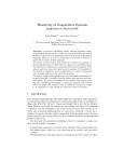


![mode d`emploi Stûv 30 [fr]](http://vs1.manualzilla.com/store/data/006452295_1-f2f8358be28b0bf58ee1c293eec3c700-150x150.png)