Download A Testbed for Networked Control Systems”

”A Testbed for Networked Control Systems”
Chengsen Song
Master’s Project
Computer Science
Department, Baylor University, August 2011
Project Report
Chengsen Song
July 27, 2011
Table of Content
1
2
Introduction ............................................................................................................................. 1-1
1.1
Background ...................................................................................................................... 1-1
1.2
What Has Been Done ....................................................................................................... 1-1
1.3
Structure of the Final Report ............................................................................................ 1-2
Related Work ........................................................................................................................... 2-1
2.1
Introduction ..................................................................................................................... 2-1
2.2
Networked Control System .............................................................................................. 2-1
2.2.1
Overview ...................................................................................................................... 2-1
2.2.2
Challenges .................................................................................................................... 2-2
2.2.3
Improve the System Performance ................................................................................ 2-3
2.3
2.3.1
Available Network Simulators ...................................................................................... 2-4
2.3.2
Available Control System Simulators ............................................................................ 2-5
2.3.3
Available Co-Simulation Tools ...................................................................................... 2-6
2.4
3
System Simulation Tools .................................................................................................. 2-4
Time Scales Theory ........................................................................................................... 2-6
Project Summary ...................................................................................................................... 3-1
3.1
Introduction ..................................................................................................................... 3-1
3.1.1
Purpose and Approach ................................................................................................. 3-1
3.1.2
Timeline........................................................................................................................ 3-2
3.1.3
Accomplishments ......................................................................................................... 3-2
3.2
Summer 2010 ................................................................................................................... 3-3
3.2.1
Overview ...................................................................................................................... 3-3
3.2.2
Objectives ..................................................................................................................... 3-3
3.2.3
What Did I Do? ............................................................................................................. 3-3
3.3
Fall Semester 2010 ........................................................................................................... 3-6
3.3.1
Overview ...................................................................................................................... 3-6
3.3.2
Objectives ..................................................................................................................... 3-6
3.3.3
What Did I Do? ............................................................................................................. 3-6
i
3.4
4
Spring Semester 2011 .................................................................................................... 3-16
3.4.1
Overview .................................................................................................................... 3-16
3.4.2
Objectives ................................................................................................................... 3-17
3.4.3
What Did I Do? ........................................................................................................... 3-17
The System Configuration ........................................................................................................ 4-1
4.1
Hardware ......................................................................................................................... 4-1
4.1.1
Computers .................................................................................................................... 4-1
4.1.2
SRV02-E servo plant ..................................................................................................... 4-1
4.1.3
UPM-1503 Power Module ............................................................................................ 4-3
4.1.4
Quanser Q4 board ........................................................................................................ 4-4
4.2
5
Software ........................................................................................................................... 4-4
4.2.1
Quanser library ............................................................................................................. 4-4
4.2.2
Matlab and Simulink..................................................................................................... 4-5
4.2.3
QNX .............................................................................................................................. 4-5
Pendulum Controller Design .................................................................................................... 5-1
5.1
Physical model ................................................................................................................. 5-1
5.1.1
Non-Linear Equations of Motion .................................................................................. 5-1
5.1.2
State-Space Representation ......................................................................................... 5-3
5.1.3
Continuous to Discrete Domain Conversion ................................................................. 5-5
5.2
Balance Controller Design ................................................................................................ 5-6
5.2.1
Full-State Feedback Controller Design ......................................................................... 5-7
5.2.2
Observer Design ........................................................................................................... 5-8
5.2.3
Controller with Reference Signal Input ...................................................................... 5-10
5.3
Simulation ...................................................................................................................... 5-14
5.3.1
Simulink Simulation Model......................................................................................... 5-14
5.3.2
Parameters ................................................................................................................. 5-15
5.3.3
Networked Control System Model ............................................................................. 5-17
5.4 Simulink Executable Model .................................................................................................... 5-19
5.5
6
Summary ........................................................................................................................ 5-22
C++ Project ............................................................................................................................... 6-1
6.1
C++ Version of the Balance Controller ............................................................................. 6-1
6.2
Varying Sampling Rate...................................................................................................... 6-4
ii
7
8
Creating your own controller ................................................................................................... 7-1
7.1
Step 1 ............................................................................................................................... 7-1
7.2
Step 2 ............................................................................................................................... 7-1
7.3
Step 3 ............................................................................................................................... 7-2
Conclusion................................................................................................................................ 8-1
8.1
Observations .................................................................................................................... 8-1
8.1.1
Comparison of Results .................................................................................................. 8-1
8.1.2
Accuracy of Simulations ............................................................................................... 8-8
8.1.3
Timing Inaccuracy ......................................................................................................... 8-9
8.1.4
Stability against Sampling Rate .................................................................................... 8-4
8.2
Conclusions and Future Work ........................................................................................ 8-13
8.2.1
Abilities of The Test Bed ............................................................................................. 8-13
8.2.2
Limitations.................................................................................................................. 8-13
8.2.3
Future Work ............................................................................................................... 8-13
Appendix A Parameter Definition
Appendix B List of Hardware and Software
Appendix C User Manual
Appendix D How to Generate Arbitrary Time Scales
iii
Last revised 07/27/2011
1
Introduction
This chapter introduces the background, purpose and results of the project.
1.1 Background
The primary purpose of the project was to develop a test bed that can facilitate research on time
scales theory and networked control theory.
Time Scales theory is a way to unify the seemingly disparate fields of discrete dynamical systems
(i.e., difference equations) and continuous dynamical systems (i.e., differential equations). Time scale
systems might best be understood as a “bridge” between discrete time and continuous time systems. A
networked control system is a control system that uses a shared network to transmit information. It is
widely used in today’s life.
To read this project report, it is assumed that the reader has a basic knowledge of control theory,
time scales theory, and networked control systems. Please refer to Chapter 3 of [1], Chapter 1 of [2],
and [3] for detailed information.
1.2 What Has Been Done
In this project we developed a test bed for modeling and simulating the time scales control and
networked control system for a rotary inverted pendulum [4]. The test bed, which allows users to
develop, simulate and run their own control algorithms, could be used to implement and verify various
theories.
The test bed provides both simulation and executable models for a rotary inverted pendulum. The
simulation models, for both the local control system and the network control system, were built using
Matlab/Simulink [5]. The simulation environment enables a user to verify the control algorithms. The
Quanser QUARC library [6] was used to create an executable model which could directly access the
1-1
Last revised 07/27/2011
hardware components. This executable model can be compiled and run on QNX [7]. To implement a
time scales control, a user could choose to use an external signal generator or to implement a controller
in C++ program would use the software timer on QNX. The test bed provides the basic structure and
interface for time scales and networked controllers. For example, researchers could incorporate time
scales theory into these models and controllers so that control algorithms could be verified or tailored
for efficiency.
1.3 Structure of the Final Report
The structure of the project report is as follows.
Chapter 2 introduces the background and the related work.
Chapter 3 is the project summary, which records what we have done from summer 2010 through
summer 2011.
Chapter 4 describes the hardware and software configuration for the test bed, which shows how to
setup the system.
Chapter 5 presents the controller design for the rotary inverted pendulum, and the implementation
of our simulation environment.
Chapter 6 summarizes the implementation of the C++ controller.
Chapter 7 introduces how to implement a new controller based on the existing example.
Chapter 8 introduces the experiment observations and conclusions.
Appendix A lists the parameters, including their symbols, names and values that are used in
defining the pendulum mathematical model.
Appendix B records the hardware and software in current configuration.
Appendix C constitutes the user manual for the test bed.
Appendix D shows how to generate arbitrary time scales using an Agilent 33220A [8] signal
generator and software.
1-2
Last revised 07/27/2011
References
[1] R. Dorf and R. Bishop, Modern Control Systems. Prentice Hall, 2008.
[2] M. Bohner and A. Peterson, Dynamic Equations on Time Scales. Birkhauser, 2001.
[3] R. A. Gupta and M. Chow, "Networked Control System: Overview and Research Trends," IEEE
Transactions on Industrial Electronics, vol. 57, pp. 2527-2535, 2010.
[4] Quanser Inc., "Rotary Experiment #08: Self Erecting Inverted Pendulum Control," .
[5] MathWorks. Matlab/Simulink. [online].
Available: http://www.mathworks.com/products/matlab/.
[6] Quanser Inc. QUARC 2.1 overview. [online].
Available: http://www.quanser.com/english/html/quarc/fs_overview.htm.
[7] QNX Software Systems. QNX neutrino RTOS. [online].
Available: http://www.qnx.com/products/neutrino-rtos/index.html.
[8] Agilent Technologies. Agilent 33220A User's Guide [online].
Available: http://cp.literature.agilent.com/litweb/pdf/33220-90002.pdf.
1-3
Last revise 07/27/2011
2 Related Work
2.1 Introduction
In this chapter, the related research on networked control system (NCS) and time scales theory is
introduced.
2.2 Networked Control System
This section introduces the research topics in NCS.
2.2.1
Overview
A control system aims to regulate the behavior of other systems. Traditional control systems are
feedback control systems in which the feedback signals are transmitted through cable or wires. When a
traditional feedback control system uses a network to connect the controller to the system, it is called a
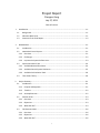
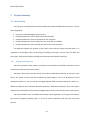
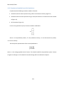
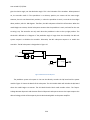
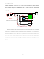
Networked Control System (NCS). More specifically, an NCS exchanges information (i.e. reference input,
plant output, control input) among control system components (sensor, controller, actuator, etc.) using
a shared network. A graphical representation of this NCS model is shown in Figure 1 [1].
Figure 1 A Conceptual Model of NCS
2-1
Last revise 07/27/2011
NCSs have been popular and widely applied for many years because of their numerous advantages,
such as reduced wiring, simpler installation, ease of system diagnosis and maintenance, and increased
system edibility.
2.2.2
Challenges
There are challenges associated with the design of an NCS. First, there are various kinds of
networks, not all of which may be appropriate for a given situation. Choosing an appropriate network
may not be trivial. Second, packages transmitted through the network may suffer delay and loss, which
influences the performance of the control system. Third, the network may be vulnerable to external
attacks. Such a security issue is very important in critical applications.
2.2.2.1 Network Technology Selection
There are many types of networks that the designer can use: Ethernet, CAN, 802.11 a/b/g,
bluetooth, ZigBee… Each type of network has its own advantages and disadvantages, so the designer
should select the most suitable one for the specific application.
2.2.2.2 Network Delay and Packet Loss Compensation
The network can introduce unreliable/nondeterministic levels of service in terms of delay, jitter,
and packet loss. These are problems that are not normally associated with traditional feedback control
systems. A common approach is to let the controller solve the problems. Based on the type of delay,
there are three solutions [2]: (1) If the delay is constant, the control target can be modeled in a state
space equation using the present input and the past inputs. Here, standard Linear Time-Invariant (LTI)
control theory can be applied. (2) If delay is variable, and the delay statistics for the network are
available, and there is a finite number of delay states, then delay can be treated as a jump-linear system
driven by an underlying Markov Chain. (3) If no delay statistics data are available, or if the delay
2-2
Last revise 07/27/2011
statistics of the states of the Markov chain does not remain constant, then either robust controller
techniques or predictor-based methods can be applied.
Usually, the controller applies compensation algorithms to compensate for the delay. Different
mathematical-, heuristic-, or statistical-based approaches are used for delay compensation in NCSs, such
as the optimal stochastic method, the queuing/buffering method, the robust control method [2-7]. This
project does not provide our own delay analysis and delay compensation. However, the test bed has the
ability to introduce arbitrary delay and packet loss rate, so that the researchers can investigate their
own various algorithms.
2.2.2.3 Network Security Enhancement
Network medium, particularly wireless medium, is susceptible to easy interception. Research in
NCS was initiated from the concern for security and convenience in hazardous environments such as
nuclear reactor power plants and military applications. In all these applications, security is of the utmost
concern. The research in this project does not include NCS security issues from the control system’s
perspective. The future research should consider these issues.
2.2.3
Improve the System Performance
The delay and packet loss problems can be addressed either within the control system, or within
the network system, or in both systems.
The first solution is to address the problem within the control system. Given the network
technology, the designer can analyze the statistics of the network. Based on this information, the
designer will design the suitable controller that can minimize the influence of the network. The second
solution is to improve the network technology to minimize the delay and loss rate, so that the network
is compatible for any type of controller. Such methods include: (1) NCS Scheduling approaches and (2)
Dynamic bandwidth allocation (DBA) approaches [1].
2-3
Last revise 07/27/2011
The above solutions only consider part of the system (either the control system or the network
system), which is not complete and efficient. Consequently, some researchers focus on co-design
approach, which provides a solution that involves improvement of both the control system and the
communication system [8-11]. The key idea of co-design approach is to optimize the control
performance by adjusting the control and the network algorithms based on network statistics. For
example, A. Chamaken presents a co-design approach for the inverted pendulum system [9]. The
authors develop and implement two controllers with control laws considering network statistics. Three
different MAC protocols are used in conjunction with two different controllers to stabilize the inverted
pendulum. The result shows that the optimal control performance can be achieved at the control layer
and the communication layer.
2.3 System Simulation Tools
System simulation tools can be used to simulate the performance of the NCS before the
implementation. Simulation is often easier than implementation. Especially when designing the
controller, many parameters in control algorithms need fine tunes. In this case, simulation can save time
and speed up the process. Since the NCS consists of the control system and network system, first we
consider using separate simulation tools for each system. However, this approach is not efficient
enough. Hence we decide to use the TrueTime toolbox as the co-simulation tool.
2.3.1
Available Network Simulators
Ns [12] is a discrete event simulator and is widely used in network research. Ns provides a
substantial support for the simulation of TCP, routing, and multicast protocols over wired and wireless
(local
and
satellite)
networks.
It
is
an
open
http://www.isi.edu/nsnam/ns/.
2-4
source
tool,
and
is
available
from
Last revise 07/27/2011
OMNeT++ [13] is a discrete event simulation environment. Its primary application is the simulation
of communication networks. OMNeT++ offers an Eclipse-based IDE and a graphical runtime
environment. OMNeT++ is free for academic and non-profit use. It is available from
http://www.omnetpp.org/.
OPNET Modeler [14] is a commercial tool developed by OPNET Inc. Modeler incorporates a broad
suite of protocols and technologies, and includes a development environment to enable the modeling of
all network types and technologies (e.g. VoIP, TCP, OSPFv3, MPLS, IPv6).
A performance comparison of recent network simulators (including ns-2, ns-3, OMNet++) can be
found in [11].
2.3.2
Available Control System Simulators
Matlab [15] is a common development environment for a variety of engineering applications.
Simulink [15] is an environment for multi-domain simulation and Model-Based Design (MBD) for
dynamic and embedded systems. Simulink provides an interactive graphical environment and a
customizable set of block libraries that can be used to design, simulate, implement, and test a variety of
time-varying systems, including communications, controls, signal processing, video processing, and
image processing. Real-Time Workshop (RTW) [16] can generate and execute C and C++ code from
Simulink diagrams. The Quanser QUARC library is based on RTW, which can generate and compile C
code for various targets. Modelica is a non-proprietary, object-oriented, equation-based language used
to model complex physical systems. OPENMODELICA [17] is an open-source Modelica-based modeling
and simulation environment intended for industrial and academic usage. Both tools can be used to
model a dynamic system. The difference is that Modelica is equation-based so a user must provide
explicit ordinary differential equations to represent a system, while Simulink uses “blocks” to represent
mathematic operations.
2-5
Last revise 07/27/2011
2.3.3
Available Co-Simulation Tools
TrueTime [18] is a Matlab/Simulink-based simulator for real-time control systems. TrueTime
facilitates the co-simulation environment of controller task execution in real-time kernels, network
transmissions, and continuous plant dynamics.
Ptolemy II [19] is an open-source software framework supporting experimentation with actororiented design. The Ptolemy Project has developed directors supporting process networks (PN),
discrete-events (DE), dataflow (SDF), synchronous/reactive(SR), rendezvous-based models, 3-D
visualization, and continuous-time models.
In this project, we chose TrueTime toolbox working with Simulink as a co-simulation tool. The main
reason of the tool selection is that Ptolemy II, with limited available resources, is not that widely used,
whereas Matlab/Simulink provides many useful tools for designing control systems, and TrueTime
toolbox works perfectly with Simulink to simulate the network system.
2.4 Time Scales Theory
In mathematics, time scale calculus is a unification of the theory of difference equations with that
of differential equations, unifying integral and differential calculus with the calculus of finite differences.
Consequently, it provides formalism for describing hybrid discrete-continuous dynamical systems [20]. It
has applications in any field that requires simultaneous modeling of discrete and continuous data.
One goal of this project is to provide a test bed, including a simulation environment and an
experiment system, for researchers to investigate the time scales theory on control systems. The time
scales theory is important because conventional control system is classified as either continuous system
or discrete system. Time scales theory helps build the connection. However, control theory on time
scales has not been much developed. Such a test bed will be useful for future researches.
Billy Jackson [21] examined linear systems theory in the arbitrary time scale setting by considering
Laplace transforms stability, controllability, observability, and realizability. Benjamin Allen [22] described
2-6
Last revise 07/27/2011
the design and implementation of a simulator and real-time controller useful for experimentation with
and demonstration of the applications of time scale control theory.
References
[1] R. A. Gupta and M. Chow, "Networked Control System: Overview and Research Trends,"
IEEE Transactions on Industrial Electronics, vol. 57, pp. 2527-2535, 2010.
[2] L. Samaranayake, M. Leksell and S. Alahakoon, "Relating sampling period and control
delay in distributed control systems," in The International Conference on Computer as a Tool
, 2005, pp. 274-277.
[3] C. Lai and P. Hsu, "Design the Remote Control System With the Time-Delay Estimator
and the Adaptive Smith Predictor," IEEE Transactions on Industrial Informatics, vol. 6, pp. 73-80,
2010.
[4] X. Dong and Q. Zhang, "Stability of singular NCS with time-varying delay and state
feedback," in International Conference on Measuring Technology and Mechatronics
Automation, 2010, pp. 473-476.
[5] E. C. Martins and F. G. Jota, "Design of Networked Control Systems With Explicit
Compensation for Time-Delay Variations," IEEE Transactions on Systems, Man, and Cybernetics,
Part C: Applications and Reviews, vol. 40, pp. 308-318, 2010.
[6] Y. Uchimura and H. Shimano, "Network based control with compensation of timevarying delay and modeling error," in 35th Annual Conference of IEEE on Industrial Electronics,
2009, pp. 3013-3018.
[7] Y. Xia, G. P. Liu, M. Fu and D. Rees, "Predictive control of networked systems with
random delay and data dropout," Control Theory & Applications, IET, vol. 3, pp. 1476-1486,
2009.
[8] A. Cervin, D. Henriksson, B. Lincoln, J. Eker and K. -. Arzen, "How does control timing
affect performance? Analysis and simulation of timing using Jitterbug and TrueTime," IEEE
Control Systems Magazine, vol. 23, pp. 16-30, 2003.
[9] A. Chamaken and L. Litz, "Joint design of control and communication in wireless
networked control systems: A case study," in American Control Conference
, 2010, pp. 1835-1840.
2-7
Last revise 07/27/2011
[10] M. S. Hasan, H. Yu, A. Carrington and T. C. Yang, "Co-simulation of wireless networked
control systems over mobile ad hoc network using SIMULINK and OPNET," IET Communications,
vol. 3, pp. 1297-1310, 2009.
[11] E. Weingartner, H. vom Lehn and K. Wehrle, "A performance comparison of recent
network simulators," in IEEE International Conference on Communications, 2009, pp. 1-5.
[12] DARPA. The network simulator - ns-2. [online]. Available:
http://www.isi.edu/nsnam/ns/.
[13] OMNeT++ Community. OMNeT++. [online]. Available: http://www.omnetpp.org/.
[14] OPNET Technologies Inc. OPNET modeler. [online]. Available:
http://www.opnet.com/solutions/network_rd/modeler.html.
[15] MathWorks. Matlab/Simulink. [online]. Available:
http://www.mathworks.com/products/matlab/.
[16] MathWorks. Real-time workshop. [online]. Available:
http://www.mathworks.com/products/simulink-coder/index.html.
[17] OpenModelica.org. OpenModelica. [online]. Available:
http://www.openmodelica.org/.
[18] Department of Automatic Control, Lund University. TrueTime toolbox. [online]. 2.0
beta 6 Available: http://www.control.lth.se/user/truetime/.
[19] UC Berkeley EECS department. Ptolemy II. [online]. Available:
http://ptolemy.berkeley.edu/ptolemyII/.
[20] Wikipedia.org. Time scale calculus. [online]. Available:
http://en.wikipedia.org/wiki/Time_scales_calculus.
[21] B. Jackson, "A General Linear Systems Theory on Time Scales: Transforms, Stability,
and Control," 2007.
[22] B. Allen, "Experimental Investigation of a Time Scales Linear Feedback Control
Theorem," 2007.
2-8
Revised 07/27/2011
3
Project Summary
3.1 Introduction
In this project, we developed a test bed to model and simulate embedded control systems. This test
bed is designed to
•
•
•
•
•
help users understand digital control systems
provide a platform for users to define their own controller
provide a platform for users to simulate their own controller
provide a platform for users to apply their own controller on hardware
provide a platform for users to design and verify time scales controllers
This document explains the purpose of the project, what and how things have been done. It is
organized in chronological order, summarizing the following semesters: summer 2010, fall 2010 and
spring 2011. Each section identifies the objectives and how those objectives were met.
3.1.1
Purpose and Approach
The primary purpose of the project is to develop a test bed that can facilitate researches on time
scales theory and networked control theory.
The Baylor University Time Scales Group [1] has done considerable researches on the time scales
theory. The theory of time scales was introduced by Stefan Hilger's in his Ph.D. dissertation [2] and
subsequent papers as a way to unify the seemingly disparate fields of discrete dynamical systems (i.e.
difference equations) and continuous dynamical systems (i.e. differential equations). Time scale systems
might best be understood as the continuum bridge between discrete time and continuous time systems.
The test bed allows users to develop and simulate control algorithms, and to generate arbitrary
time scales (to regulate sampling rates), so it can be used to implement and verify the time scales
theories.
3-1
Revised 07/27/2011
The secondary purpose of this project is to understand digital control systems. Also, this project the examples and the project report - should be helpful for people who are learning control theory.
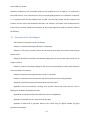
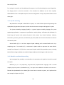
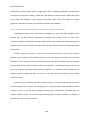
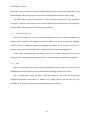
We have chosen the rotary inverted pendulum as an example system because it is an unstable
system and it is a commonly-used example in the literature. In particular, we use the Quanser SRV02 [3]
pendulum system, which consists of a horizontal arm, a vertical pendulum, a gear chain, and a DC servo
motor (as shown in Figure 1). The detailed system configuration will be introduced in Chapter 4.
Figure 1 SRV02 Rotary Inverted Pendulum System
3.1.2
•
•
•
3.1.3
Timeline
This project started during the summer 2010 semester when we set up the hardware and
indentified the research problem.
In the fall 2010 semester, we analyzed the dynamic model, designed and simulated the
pendulum controller in Simulink. Also, we re-configured the system with the controller running
QNX.
In the spring 2011 semester, we implemented the controller in Simulink and then in C++.
Accomplishments
We have completed the following tasks:
•
•
•
Work through Quanser lab 0 [4], lab 1 [5], lab 2 [6], lab 3 [7], lab 7 [8], lab 8 [9]
Identify relevant research papers
Understand how to model the pendulum system using Matlab/Simulink
3-2
Revised 07/27/2011
•
•
•
Understand how to design the controller
Construct the controller in Simulink and then simulate the system
Construct the controller in C++
3.2 Summer 2010
3.2.1
Overview
We started the project in the summer of 2010. Dr. Eisenbarth set up the rotary pendulum hardware
for the Quanser SRV02, with one PC running Windows XP for both developing and running the
controller. Quanser provides eight labs that demonstrate how to utilize the hardware and software. I
worked on doing these labs, as well as indentifying the research problems.
3.2.2
Objectives
Our objectives during that time were to
•
•
•
•
•
•
3.2.3
Understand how to use the Quanser software and hardware
Carry out the rotary pendulum experiments provided by Quanser
Investigate SysML [10] modeling
Investigate Modelica [11] modeling and simulation
Investigate model transformation using VIATRA [12]
Read papers on network control system and identify research problems
What Did I Do?
3.2.3.1 Quanser Labs
On the software side, I followed the Quanser manual [3] and did Lab 0-3, and 7-8. This helped me
understand how to install Quanser software, how to create a Quanser Simulink model, how to configure
the target machine, and how to compile and run a model.
On the hardware side, I worked with Dr. Eisenbarth to setup the hardware. Initially, we had only
one Windows XP PC used for both developing and running the controller. However, we found that
sometimes the pendulum fell down after a short time. Probably it is because that Windows XP is not a
real time operating system. Therefore, Dr. Eisenbarth added a second PC running the QNX Neutrino [13]
real time operating system. This is the current system configuration, in which the QNX computer is only
3-3
Revised 07/27/2011
for running the controller and the Windows XP computer is only for developing the control algorithms.
The design process is that the controller is first simulated on Windows XP, and then compiled,
downloaded and run on the QNX computer. Since this configuration is setup, the pendulum does not fall
down again.
3.2.3.2 SysML modeling
We planned to use SysML to describe the system, so I read the book Systems Engineering with
SysML/UML [14] (particularly Chapter 4) which describes the basic concepts and diagrams in SysML.
The Systems Modeling Language (SysML) is a general purpose modeling language for system
engineering applications. It supports the specification, analysis, design, verification and validation of a
broad range of systems and systems-of-systems. Such systems may include hardware, software,
information, processes, personnel, and facilities [10]. Here SysML can be used to describe the structure
of a control system.
Artisan Studio [15] is a tool that supports SysML modeling and I became familiar with it by
completing one of its tutorials [16]. I constructed a SysML model to represent the water distiller
example from Chapter 15 of [14]. Also, I constructed a SysML model of the pendulum system, including
Block Definition Diagram (BDD), Internal Block Diagram (IBD), activities diagrams and state charts.
3.2.3.3 Modelica and Simulink modeling
We investigated the possibility to use Modelica (in conjunction with SysML) or Simulink to model
the system.
Modelica [17] is a non-proprietary, object-oriented, equation-based language used to model
complex physical systems. OpenModelica [11] is an open source Modelica simulation environment. I
followed the OpenModelica Users Guide [18] to learn how to simulate a system, and I replicated the
tank example in Chapter 15 of [19].
3-4
Revised 07/27/2011
Simulink [20] is an environment for multi-domain simulation and model-based design for dynamic
and embedded systems. It provides an interactive graphical environment and a customizable set of
block libraries that enable users to design, simulate, implement, and test various applications, including
communications, controls, signal processing, video processing, and image processing.
Both tools can be used to model a dynamic system. The difference is that Modelica is equation
based so that a user must provide explicit ordinary differential equations to represent a system. On the
contrary, Simulink uses blocks to represents mathematic operations.
3.2.3.4 VIATRA2
Model transformation is important in model-driven engineering. In this project, model
transformation is used to transfer the Simulink model into an executable binary code. So how to do
model transformation is one of the research problems to be investigated.
VIATRA2 (VIsual Automated model TRAnsformations) [12] framework provides a general-purpose
support for the entire life-cycle of engineering model transformations. In particular, it provides a means
to uniformly represent models and metamodels, and a high performance transformation engine. To
understand the framework, I read the VIATRA 2 Model Transformation Framework User’s Guide [21],
Chapter 1-3. And I did VIATRA2 hello world and Transforming UML activity diagram into a Petri net
tutorial. But at current stage, model transformation has not been done yet. The VIATRA2 tool has not
been used.
3.2.3.5 Other relevant research
Thomas Johnson’s thesis, Integrating Models and Simulations of Continuous Dynamic System
Behavior into SysML [22], describes how SysML and Modelica can be used in concert. The objective of
his research was to use graph patterns and transformation rules to integrate models of continuous
3-5
Revised 07/27/2011
dynamic system behaviors (represented using Modelica) with SysML models. This would provide a more
comprehensive modeling approach.
I used IEEExplore to locate papers relevant to my project based on the keyword “Networked
Control System” (NCS). I selected about 20 papers, read through each one, and selected the interesting
ones and added them to my RefWorks repository [23-28]. In particular, I found that NCS co-design,
which considers the characteristics of both the network and control system and solves the problem as
an integrated system, is very interesting [29-33] and focused on it during the fall 2010 semester.
3.3 Fall Semester 2010
3.3.1
Overview
During the fall 2010 semester, I set up the rotary pendulum simulation environment in Simulink and
developed the controller. The simulation results demonstrated that the controller could successfully
balance the pendulum. I also investigated how to simulate an Network Control System (NCS). After
investigating several different tools [11, 20, 34-39], I finally chose the TrueTime toolbox [35].
3.3.2
Objectives
The objectives of the fall semester were to
•
•
•
•
•
•
3.3.3
Understand how to model the dynamics of the rotary pendulum
Understand the Quanser Simulink model
Implement the Simulink model that simulates the balance controller
Investigate networked control systems
Implement an NCS controller for the rotary pendulum
Determine how to use the TrueTime toolbox to simulate wireless networks
What Did I Do?
3.3.3.1 Investigate NCS simulation tools
I searched the Internet for network and control systems simulation tools and found several relevant
types: co-simulation tools (e.g., TrueTime [35], Ptolemy II [38], PiccSIM [39]), network simulators (e.g.,
3-6
Revised 07/27/2011
OPNET [37], NS-2 [34], NS-3 [34], OMNeT++ [36]), and control system simulation tools (e.g., Simulink
[20] and Modelica [11]).
I evaluated these tools, based on their capabilities: the related programming languages, the
operating system that is assumed, the compatibilities of working with other tools and required
resources. After evaluating each tool, I found that the TrueTime toolbox would work well for NCS cosimulation, because the TrueTime toolbox provides Simulink blocks that are targeted for network
simulation, making it easy to set up an NCS environment in Simulink.
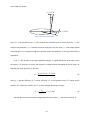
3.3.3.2 Practice Simulink modeling
I replicated the tank example from page 385 of Principles of Object-Oriented Modeling and
Simulation with Modelica 2.1 [19]. The original model is represented in Modelica, and I created an
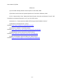
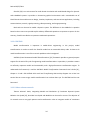
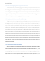
equivalent model in Simulink. Figure 2 shows the structure of the tank system. Liquid enters the tank
through a pipe from a source (on the left), and leaves the tank via another pipe (on the right) at a rate
controlled by a valve. The liquid level in the tank must be maintained at a fixed level as closely as
possible, no matter what the input flow is.
Figure 2 A Tank System
model Tank
ReadSignal
ActSignal
LiquidFlow
LiquidFlow
parameter
parameter
parameter
Real
tSensor
"Connector, sensor reading tank level (m)";
tActuator "Connector, actuator controlling input flow";
qIn
"Connector, flow (m3/s) through input valve";
qOut
"Connector, flow (m3/s) through output valuve";
Real area(unit = "m2")
= 0.5;
Real flowGain(unit = "m2/s") = 0.05;
Real minV = 0, maxV = 10;// Limits for output valve flow
h(start = 0.0, unit = "m") "Tank level";
equation
assert(minV >= 0, "minV - minimum Valve level must be >= 0");
3-7
Revised 07/27/2011
der(h) = (qIn.lflow - qOut.lflow)/area;
// Mass balance
equation
qOut.lflow = LimitValue(minV, maxV, -flowGain*tActuator.act);
tSensor.val = h;
end Tank;
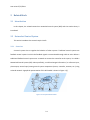
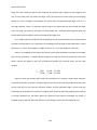
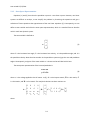
Figure 3 A Modelica Model
The Modelica source code for the tank is shown in Figure 3. Note that each physical object is
represented as an object (or variable) and equations represent continuous behaviors.
The out flow valve is controlled by a PI controller to keep the height of the liquid at 0.25 meters,
where the parameters for the PI controller are P = 2 and I = 0.1. The control system diagram is shown in
Figure 4.
Figure 4 A Tank Simulink Model with a Continuous PI Controller
To model the system, I first created the tank subsystem. Here I replaced the ordinary differential
equations in Modelica with Simulink blocks. The corresponding equation and blocks are marked in
Figure 5 , with the associated equations shown in the figure.
3-8
Revised 07/27/2011
der(h) = (qIn.lflow - qOut.lflow)/area;
qOut.lflow = LimitValue(minV, maxV, -lowGain*tActuator.act);
Figure 5 Simulink Subsystem
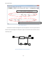
A continuous PI controller was designed to control the liquid level in the tank. Figure 6 shows the
Simulink control system diagram. The Subsystem in Figure 6 is connected to the PI controller to form a
closed-loop system.
qIn
Step
Scope
qOut
tActuator
tSensor
Subsystem
Scope1
PI(s)
0.25
Add
PID Controller1
Constant
Figure 6 Simulink Model of the Local Control System
3-9
Revised 07/27/2011
tank liquid height
0.7
0.6
height(m)
0.5
0.4
0.3
0.2
0.1
0
0
50
100
150
time(s)
200
250
300
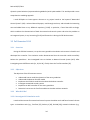
Figure 7 Simulation Result of the Local Control System
To simulate the tank system, we assume that there is an input liquid flow, which is the input signal
(i.e., qin). Assume that the input flow maintains at 0.02 m3/s from 0 to 150 second, and then increases
to 0.06 m3/s after 150 second. The height of liquid in the tank is shown in Figure 7. At t = 0, the height is
0, and the liquid begins to flow into the tank. After the height is over 0.25 m, the PI controller adjusts
the valve to maintain the height at 0.25 m. At t = 150, the input liquid flow increases, so here is an
overshoot in the height. But the PI controller maintains the liquid level to 0.25 m.
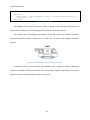
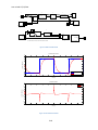
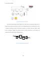
After successfully creating the Simulink model and running the simulation, I embedded a TrueTime
network block in the model and completed an NCS, as shown in Figure 8. The upper collection of blocks
represents the tank, sensor and actuator system, and the lower collection of blocks represents the
controller system. These two collections communicate through TrueTime send and receive blocks, which
are configured to use the Ethernet protocol. The tank system uses a Sensor Trigger to sample the liquid
height, and sends the liquid height information through the TrueTime (Sensor) block. On the controller
side, the TrueTime Receiver (Controller) block receives the data, calculates the control signal, and sends
it through the TrueTime Send (Controller) block. The TrueTime Receive (Actuator) block receives the
3-10
Revised 07/27/2011
control signal, and adjusts the actuator accordingly. The simulation result is shown in Figure 9, which is
identical to the simulation result of local control system in Figure 7.
qIn
250
Clock
qOut
tActuator
Step
Display
tSensor
Scope
Subsystem
Data
1: 2
Scope1
Trigger
1: 2 Data
Sensor
Trigger
TrueTime Send
(Sensor)
TrueTime Receive
(Actuator)
1 Schedule
Network
Schedule
r
TrueTime Network
0.25
PI(z)
Data
Constant
Add
1: 3
Discrete PID Controller
Trigger
Data
1: 3
TrueTime Send
(Controller)
Trigger
Computational
Delay
TrueTime Receive
(Controller)
Figure 8 Simulink Model of the Networked Control System
tank liquid height
0.7
0.6
height(m)
0.5
0.4
0.3
0.2
0.1
0
0
50
100
150
200
250
time(s)
Figure 9 Simulation Result of the Networked Control System
3.3.3.3 Model Rotary pendulum and Design Controller
At the beginning of the fall semester, I read the Quanser manual [9] to understand how to model
the pendulum dynamics. The dynamic equations can be constructed by using the Lagrangian [40]. I
3-11
Revised 07/27/2011
created a non-linear Simulink model (Figure 11) based on the dynamic equations to represent the
pendulum system. The pendulum system is a non-linear system. But in order to simplify the problem, we
linearize the equations by assuming that the pendulum angle is close to 0 when balanced. This results in
a state space representation, which is a linear system – an approximation of the actual non-linear
system.
Figure 10 Simulink Rotary Pendulum Model
The performance of the linear approximation can be analyzed by comparing it with the respective
non-linear Simulink model. I created the first Simulink model (Figure 10) that utilizes the non-linear
model. Initially, the simulation initial condition sets the pendulum angle to 0.01 rad, which is a small
non-zero value representing an unbalanced condition. The simulation sets the input to 0 volts,
simulating the free-falling nature of the pendulum. Similarly, I created the second Simulink model with
the non-linear subsystem replaced by a state space subsystem. After running the simulations, I
compared the outputs (arm position and pendulum position) of the two models. The result should
indicate that the output of the linear model matches the non-linear model when the pendulum angle is
small, and the output of the linear model deviates from the non-linear model when the pendulum angle
becomes large. However, my non-linear block simulation result showed an unchanged pendulum angle,
which was incorrect. Since the non-linear model was not used in the project, I did not investigate this
issue further.
3-12
Revised 07/27/2011
Figure 11 Non-linear Pendulum Model
3.3.3.4 Design the Controller
During the fall 2010 semester, I took the control theory class, ECL 4337, which focused on the
design of continuous control systems, using the textbook Modern Control Systems [41]. Since this
project requires knowledge of digital control systems, I referenced the book Digital Control of Dynamic
Systems [42], which describes how to design a digital feedback control system including a controller and
an observer.
3-13
Revised 07/27/2011
3.3.3.5 Implement Simulink Controller Simulations
I implemented the following simulation models in Simulink.
•
Simulation with the motor dynamics using a filter to estimate the velocity (Figure 12)
•
Simulation with the motor dynamics using a state space observer to estimate the state variable
x (Figure 13)
•
NCS simulation (Figure 14)
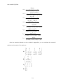
For the rotary pendulum system, the state variable x is defined as
θ 
 
α
x= 
 θ 
 
 α 
where θ is the pendulum position, θ is the pendulum velocity, α is the horizontal arm position,
α is the arm velocity.
The state-space representation of the inverted pendulum is

x=Ax+B
u
y=Cx+Du
where u is the voltage applied to the DC motor. The Simulink model for the pendulum system is shown
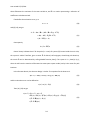
in Figure 12 and Figure 13. The details of controller design will be introduced in Chapter 5.
3-14
Revised 07/27/2011
2
-Kreference signal
3
tau (N.m)
Vi (V)
Vi (V)
RefGain
y(n)=Cx(n)+Du(n)
x(n+1)=Ax(n)+Bu(n)
Vm (V)
th_dot (rad/s)
Select
theta_dot
y
y
Scopes
rotary pendulum system
Actuator Electrical
Dynamics
Torque-Voltage
Actuator Dynamics
y _d
4
1
u
5
6
xhat
K*u
Xhat
Control gain K
Y
Observer
Figure 12 Simulink Model with a Filter Observer
For our system, however, the encoder only has access to θ and α , and is missing θ and α , so an
observer is needed to estimate the velocities, θ and α . The observer can be implemented in two ways.
The observer (subsystem 5) in Figure 12 utilizes a differentiator and a filter to estimate the velocities,
while the observer (subsystem 5) in Figure 13 uses a state space observer to estimate the velocities. The
filter observer is specific to this application, but I need to investigate more general cases. Therefore, I
decided to use the state space observer.
2
1
-Kreference signal
y _d
3
4
tau (N.m)
Vi (V)
Vi (V)
RefGain
Vm (V)
th_dot (rad/s)
Select
theta_dot
Actuator Electrical
Dynamics
Torque-Voltage
Actuator Dynamics
y(n)=Cx(n)+Du(n)
x(n+1)=Ax(n)+Bu(n)
rotary pendulum system
5
6
Y
K*u
Xhat
u
Control gain K
State Space Observer
Figure 13 Simulink Model with a State-Space Observer
3-15
y
Scopes
Revised 07/27/2011
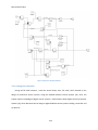
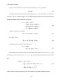
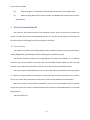
The above models (Figure 12 and Figure 13) represent local control systems. To simulate a
networked control system and investigate its performance, I created an NCS model (Figure 14) using a
TrueTime Network block, which can be configured to be one of several networks (e.g. Ethernet, CAN),
and various parameters, such as bit rate, loss rate. In Figure 14, subsystems 1-6 are the same as the local
control system (Figure 12 and Figure 13). But the system now is divided into two isolated systems: the
controller system and the pendulum system. In the pendulum system (blocks 1-4, 7, 10), the sensors
(block 7) get the position information and sends it to the controller, where the data rate is controlled by
the sensor trigger. The pendulum receiver (block 10) receives the control signal, and writes it to the
actuator. In the controller system (subsystems 5, 8, 9), the controller receiver (block 8) receives the
position information, calculates the control signal, and sends it back to the actuator through controller
sender (block 9).
3
2
1
4
X_d
-K-
tau (N.m)
u
Vi (V)
Vi (V)
Vm (V)
th_dot (rad/s)
reference signal
RefGain
Actuator Electrical
Dynamics1
Torque-Voltage
Actuator Dynamics
y(n)=Cx(n)+Du(n)
x(n+1)=Ax(n)+Bu(n)
rotary pendulum system
X
Scopes1
Data
1: 2
1: 2 Data
Trigger
Sensor
Trigger
TrueTime Receive
(Actuator)
10
TrueTime Send
(Sensor)
7
5
Select
theta_dot
Data
1: 3
Trigger
Y
6
Xhat
u
K*u
Data
State Space Observer
Control gain K
1: 3
Trigger
1 Schedule
Network
Schedule
TrueTime Receive
(Controller)
TrueTime Send
9
8
TrueTime Network
11
Figure 14 Simulink model of NCS
3.4 Spring Semester 2011
3.4.1
Overview
During the spring 2011 semester, I implemented the controller that I had simulated during the
previous semester. The first step was to implement it in Simulink. After I got the controller working, I
3-16
Revised 07/27/2011
found that Simulink had the limitation that the sampling rate could not be varied. This restriction had to
be overcome because we wanted to use the time scales theory, which would require the sampling rate
to be altered during runtime. Dr. Eisenbarth suggested that we attach a signal generator (i.e. Agilent
33220A) to the external interrupt pin on the Q4 board. We could then use the Agilent software to
generate arbitrary time scales. This solution allowed us to predefine several time scales, which could
then be chosen at runtime.
However, the time scales could not be changed after it is downloaded to the signal generator. So I
implemented a software solution, which was a C++ representation of the controller running on QNX.
QNX provides software timers that can be used in the C++ project. When a timer expires, the program
directly accesses the Q4 board and calculates the control signal. So we can set the timer expiration time
at each step, which gives us the flexibility to change the sampling rate.
During this time, to understand time scales theory on control systems, I read Benjamin Allen’s
thesis, Experimental investigation of a time scales linear feedback control theorem [43], and Billy
Jackson’s dissertation, A General Linear Systems Theory on Time Scales: Transforms, Stability, and
Control [44].
3.4.2
Objectives
The objectives of this semester were to
•
•
•
•
3.4.3
Implement my controller in Simulink
Implement my controller in C++
Study the time scales theory
Investigate the stability of switched systems
What Did I Do?
3.4.3.1 Implement the balance controller in Simulink
I implemented an executable model in Simulink, which can be compiled, downloaded and run on
QNX. However, when I first implemented the controller the controller did not balance the pendulum. It
3-17
Revised 07/27/2011
seemed that the motor did not output enough torque. After investigating the Quanser Lab 8 and each
sub-system in the Quanser example, I found that I had failed to include the motor dynamic sub-system
in my model. After adding the motor dynamics sub-system, which converts the torque to a voltage
signal that is applied to the motor, the controller can balance the pendulum.
3.4.3.2 Read Ben’s thesis and Jackson’s dissertation on time scales theory
I read Benjamin Allen’s thesis, Experimental investigation of a time scales linear feedback control
theorem [43], and Billy Jackson’s dissertation, A General Linear Systems Theory on Time Scales:
Transforms, Stability, and Control [44]. Based on Ben’s Matlab code, I implemented a Matlab program to
simulate the time scales controller. However, there were two problems when we considered the time
scales control.
(1) How to design the observer. Currently time scales control theory can only solve full-state
feedback control problem. In the pendulum system, we only have position information, but no velocity
information. So our system has only partial state information. Also, the conventional observer technique
generally does not work when using time scales. In my simulation, I calculated the observer matrices at
each step, using the conventional pole placement algorithm. The simulation result showed that the
pendulum would converge only after a long time. At this point we lack the theory so this problem
remains unsolved.
(2) How to vary the sampling rate while a model is running. To use time scales control, we need to
vary the sampling rate. In Simulink, the sampling rate is a system parameter that should be set before
simulation. Once it is set, we cannot change it. Besides, when compiled into executable code, the
Quanser software creates a thread with fixed scheduling period on QNX. Therefore, it is difficult to
generate and use time scales in Simulink.
3-18
Revised 07/27/2011
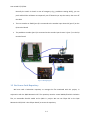
3.4.3.3 Use external signal generator to generator time scales
To solve Problem Two, we attached a signal generator directly to the Q4 extension board to control
the sampling rate via the external interrupt pin on the Q4 extension board. To utilize this signal, the
sensor reading block must be configured to use an external interrupt as the clock. After these hardware
changes were made, we did experiments to determine whether the Simulink model’s sampling rate was
in fact controlled by the external interrupt signal, and the answer was yes.
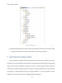
3.4.3.4 Implement the balance controller on QNX using C+
Though the time scales can be generated by external signal generator, we could not directly control
the signal generator from the Simulink model. Therefore, I solved Problem Two by implementing a C++
version of the controller mimicking the Simulink model, where the time scales was generated by
software timer. I developed the project using QNX Momentics IDE. To achieve a varying sampling rate, I
use a software timer to control the sampling rate. The QNX provides software timers that can be set.
When the timer expires, the OS sends a signal to the controller program. Upon receiving the signal, the
program directly accesses the Q4 board to read sensor data and calculates the control signal. We can set
the timer expiration time after it expires so that the sampling rate can vary. This gives us the flexibility to
generate time scales while the controller is running. At the beginning, I had some difficulty compiling the
project. But after I set the correct library/header path, and linked to the correct Quanser library, the
compilation was successful.
3.4.3.5 Investigate the switch system stability
One of our objectives is to investigate the stability of the system when it switches from a stable
state to an unstable state, and vice versa. From time scale theory, we know that there exists a µ max and
corresponding Hilger circle associated with the control system. µ max is the largest sampling period that a
digital controller can use and still guarantee stability. Assume that the system’s graininess is µ , the
3-19
Revised 07/27/2011
Hilger circle has a diameter equal to the reciprocal of graininess and is tangent to the imaginary axis
[45]. If the system poles stay within the Hilger circle, the system will remain stable. As the sampling
period ( µ ) varies, the Hilger circle changes. The system poles may go outside the Hilger circle if µ is
too large. However, there is a conjecture that as long as the system does not stay outside the Hilger
circle “too long”, the system is still stable. To demonstrate this, I simulated what happened when the
system switched forth and back inside and outside of the Hilger circle.
First, I used the Simulink model to find the sampling rates (1) that would balance and (2) that would
not balance the pendulum. Let Ts represents the sampling period. By doing several experiments, I found
that when Ts <= 10 ms, the pendulum is stable, and when Ts = 20 ms the pendulum is unstable.
Second, I investigated the case where the control system switched between the stable and unstable
case. For the simulation, I created a Matlab program to model the switching mechanism, where the
switch criterion was based on the norm of difference between the reference vector and the state
variable.
5ms if || ref − x ||> 0.04
Ts = 
20ms if || ref − x ||≤ 0.04
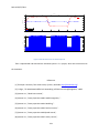
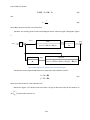
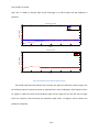
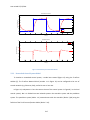
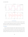
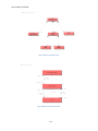
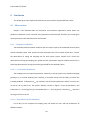
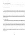
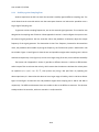
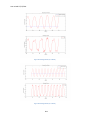
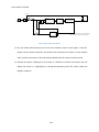
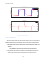
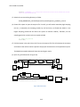
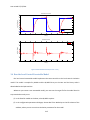
Figure 15 shows the position and Ts when the horizontal arm is tracking a square-wave reference
input with amplitude 0.1 rad. Here, the above figure shows the arm position and pendulum position. We
can see that the arm can track the reference position, and the pendulum angle is within 0.04 rad,
indicating that the pendulum is balanced. The figure below shows the switching sampling period, where
Ts switches between 5ms and 20ms. When the reference input remains unchanged, the system is
sampled at 20ms. However, when the reference input changes, system must be sampled at 5ms.
3-20
Revised 07/27/2011
positions
0.15
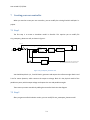
0.1
positions(rad)
0.05
0
-0.05
-0.1
-0.15
-0.2
arm position
pendulum position
0
2
4
6
8
10
12
14
8
10
12
14
Time (s)
Sampling period(µ)
0.02
0.018
0.016
0.014
µ(ms)
0.012
0.01
0.008
0.006
0.004
0.002
0
0
2
4
6
Time (s)
Figure 15 Simulation Result of the Switched System
Then I implemented and executed this switched system in C++ project, which was consistent with
the simulation.
References
[1] The Baylor University Time Scales Group. [online]. Available: http://timescales.org/.
[2] S. Hilger, "Ein MasskettenkalkÄul mit Anwendung auf Zentrumsmannigfaltigkeiten," 1988.
[3] Quanser Inc., "SRV02 user manual," .
[4] Quanser Inc., "Rotary Experiment #00: QuaRC Integration," .
[5] Quanser Inc., "Rotary experiment #01: Modeling," .
[6] Quanser Inc., "Rotary experiment #02: Position control," .
[7] Quanser Inc., "Rotary experiment #03:Speed control," .
[8] Quanser Inc., "Rotary experiment #07: Gantry control," .
3-21
Revised 07/27/2011
[9] Quanser Inc., "Rotary Experiment #08: Self Erecting Inverted Pendulum Control," .
[10] SysML.org. SysML. [online]. Available: http://sysml.org/.
[11] OpenModelica.org. OpenModelica. [online]. Available: http://www.openmodelica.org/.
[12] VIATRA2 Developer Team. VIATRA2. [online]. Available:
http://www.eclipse.org/gmt/VIATRA2/.
[13] QNX Software Systems. QNX neutrino RTOS. [online]. Available:
http://www.qnx.com/products/neutrino-rtos/index.html.
[14] T. Weilkiens, Systems Engineering with SysML/UML. USA: MORGAN KAUFMANN, 2006.
[15] Atego. Artisan studio. [online]. Available: http://www.atego.com/.
[16] Artisan Software, Artisan Studio Studio Tutorial. 2009.
[17] The Modelica Association. Modelica. [online]. Available: https://www.modelica.org/.
[18] P. Fritzson. (2009, OpenModelica users guide. [online]. Available:
http://www.ida.liu.se/labs/pelab/modelica/OpenModelica/releases/1.6.0/doc/OpenModelicaUsersGuid
e.pdf.
[19] P. Fritzson, Principles of Object-Oriented Modeling and Simulation with Modelica 2.1. WileyIEEE Press, 2004.
[20] MathWorks. Matlab/Simulink. [online]. Available:
http://www.mathworks.com/products/matlab/.
[21] OptXware Research & Development LLC., "The Viatra-I Model Transformation Framework
Users’ Guide," .
[22] T. Johnson, "Integrating Models and Simulations of Continuous Dynamic System Behavior into
SysML," 2008.
[23] G. P. Liu, D. Rees and S. C. Chai. Design and practical implementation of networked predictive
control systems. Presented at Networking, Sensing and Control, 2005. Proceedings. 2005 IEEE.
[24] L. Wu and X. Hao, "A novel optimal controller design and evaluation for networked control
systems with time-variant delays," in 2010 International Conference on Measuring Technology and
Mechatronics Automation, 2010, pp. 261-264.
[25] A. Onat, T. Naskali, E. Parlakay and O. Mutluer. (2010, Control over imperfect networks: Model
based predictive networked control systems. IEEE Transactions on Industrial Electronics (99), pp. 1-1.
3-22
Revised 07/27/2011
[26] N. J. Ploplys, P. A. Kawka and A. G. Alleyne. (2004, Closed-loop control over wireless networks.
Control Systems Magazine, IEEE 24(3), pp. 58-71.
[27] Y. Wang, S. X. Ding, H. Ye and G. Wang, "A New Fault Detection Scheme for Networked Control
Systems Subject to Uncertain Time-Varying Delay," IEEE Transactions on Signal Processing, vol. 56, pp.
5258-5268, 2008.
[28] Y. Zhang, Q. Zhong and L. Wei, "Stability of networked control systems with communication
constraints," in Control and Decision Conference, 2008. CCDC 2008. Chinese, 2008, pp. 335-339.
[29] A. Cervin, D. Henriksson, B. Lincoln, J. Eker and K. -. Arzen, "How does control timing affect
performance? Analysis and simulation of timing using Jitterbug and TrueTime," IEEE Control Systems
Magazine, vol. 23, pp. 16-30, 2003.
[30] X. Diao, "ME 452 course project II rotary inverted pendulum," 2006.
[31] A. Chamaken and L. Litz, "Joint design of control and communication in wireless networked
control
systems:
A
case
study,"
in
American
Control
Conference
, 2010, pp. 1835-1840.
[32] M. S. Hasan, H. Yu, A. Carrington and T. C. Yang, "Co-simulation of wireless networked control
systems over mobile ad hoc network using SIMULINK and OPNET," IET Communications, vol. 3, pp. 12971310, 2009.
[33] E. Weingartner, H. vom Lehn and K. Wehrle, "A performance comparison of recent network
simulators," in IEEE International Conference on Communications, 2009, pp. 1-5.
[34] DARPA. The network simulator - ns-2. [online]. Available: http://www.isi.edu/nsnam/ns/.
[35] Department of Automatic Control, Lund University. TrueTime toolbox. [online]. 2.0 beta 6
Available: http://www.control.lth.se/user/truetime/.
[36] OMNeT++ Community. OMNeT++. [online]. Available: http://www.omnetpp.org/.
[37] OPNET Technologies Inc. OPNET modeler. [online]. Available:
http://www.opnet.com/solutions/network_rd/modeler.html.
[38] UC Berkeley EECS department. Ptolemy II. [online]. Available:
http://ptolemy.berkeley.edu/ptolemyII/.
[39] Wireless Sensor Systems group Aalto University. PiccSIM. [online]. Available:
http://wsn.tkk.fi/en/software/piccsim/.
[40] M. Calkin, Lagrangian and Hamiltonian Mechanics. World Scientific, 1996.
[41] R. Dorf and R. Bishop, Modern Control Systems. Prentice Hall, 2008.
3-23
Revised 07/27/2011
[42] G. Franklin and D. Powell, Digital Control of Dynamic Systems. Addison-Wesley publishing
company, 1980.
[43] B. Allen, "Experimental Investigation of a Time Scales Linear Feedback Control Theorem," 2007.
[44] B. Jackson, "A General Linear Systems Theory on Time Scales: Transforms, Stability, and
Control," 2007.
[45] Baylor Time Scales Group. The Hilger complex plane. [online]. Available:
http://marksmannet.com/TimeScales/Time_Scales_Tutorial/index_files/5.html.
3-24
Last revised 07/27/2011
4
The System Configuration
The hardware and software that we have used in the project are described in this chapter. For a
detailed list of the hardware and software (plus contact information), please refer to Appendix B.
4.1 Hardware
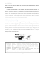
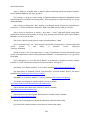
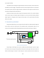
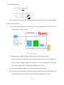
The hardware includes the following components: a host computer (Host) running Windows 7 (on
which a virtual machine was installed to run Windows XP), a target computer (Target) running QNX
Neutrino Realtime Operating System, a Quanser Q4 data acquisition board and a terminal board, a UPM1503 Power Module, and a SRV02-E servo plant and pendulum (Rotary Pendulum).
Figure 1 Hardware Configuration
4.1.1
Computers
The Host is used to develop the control algorithm and to run a simulation, using the
Matlab/Simulink environment. By utilizing the Quanser software, a Simulink model can be compiled on
the Host computer, and the executable can be downloaded and run on the Target. The Target runs the
QNX realtime operating system and is used to execute the controller.
4.1.2
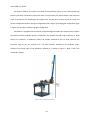
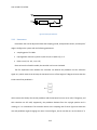
SRV02-E Servo Plant
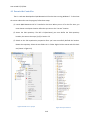
The Rotary Pendulum module is from Quanser Corporation. It consists of a horizontal arm and a
vertical pendulum attached to a Quanser SRV02-E servo plant (as shown in Figure 2).
4-1
Last revised 07/27/2011
The Quanser SRV02-E servo plant is the base of the pendulum system. It has a metal frame that
houses a gear drive connected to a DC servo motor. The horizontal arm, which rotates in the horizontal
plane, is mounted on the outside gear of the gear drive. The gear drive is driven by the DC motor and
has two configuration options: low-gear configuration (left in Figure 3) and high-gear configuration (right
in Figure 3). This project used the high-gear configuration.
The SRV02-E is equipped with two optical incremental digital encoders that measure the horizontal
arm position and the pendulum position, respectively. The encoders provide a high resolution, i.e. 4096
counts per revolution, in quadrature mode. The encoder attached to the arm shaft measures the
horizontal angle of the arm, defined as θ . The other encoder, attached to the pendulum hinge,
measures the vertical angle of the pendulum, defined as α (shown in Figure 2). Both α and θ are
measured in radians.
Figure 2 Rotary Inverted Pendulum
4-2
Last revised 07/27/2011
Figure 3 Gear Configuration
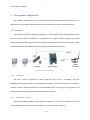
4.1.3
UPM-1503 Power Module
The UPM-1503 (Universal Power Module) contains a ±12 volt power supply, analog sensor input
and power amplified analog output. It is used to drive the DC motor.
Figure 4 UPM-1503
4.1.4
Quanser Q4 board
The Quanser Q4 board is really two boards: a Data Acquisition (DAQ) board (shown in Figure 5) and
an external terminal board (shown in Figure 6). These boards connect the controller to the pendulum
system. The DAQ board is installed on the Target’s PCI bus, and is connected to the external terminal
board via a flat cable. The terminal board provides ports for digital encoder input, analog input, analog
4-3
Last revised 07/27/2011
output, and digital input. For this project, we have only used the digital encoder input and the analog
input ports.
Figure 5 Quanser Q4 Data Acquisition Board
Figure 6 Quanser Q4 Terminal Board
4.2 Software
4.2.1
Quanser Library
Quanser QUARC library allows control prototyping and hardware-in-the-loop testing. It is integrated
with Simulink and the Real Time Workshop (RTW). The QUARC library extends the code generation
capabilities of RTW by adding a new set of Targets, such as Windows and QNX x86. The Target OS setting
determines the code generated by the RTW. This allows the user to compile the C source code
4-4
Last revised 07/27/2011
generated from the model, to link it with the appropriate libraries for the particular Target platform, and
to download the code to the Target via an Ethernet connection between the Host and the Target.
The QUARC library supports data acquisition cards from other manufacturers, such as National
Instruments. The library also provides a driver for the Q4 board so that the controller can use high-level
functions from the QUARC library to complete low-level IO tasks.
4.2.2
Matlab and Simulink
We have used Matlab as our basic development platform because the Quanser hardware and
software works seamlessly with Matlab and Simulink. Matlab is a textual programming language,
whereas Simulink is a graphical programming language that allows the user to define a system as a
collection of interconnected “building blocks”, where the blocks are manipulated graphically.
In this project, we developed our own Simulink version of a controller, which then served as the
architecture for a controller that we implemented in C++ (executed without using Matlab or Simulink).
4.2.3
QNX
QNX is a realtime operating system (RTOS) from QNX Software Systems. We are currently running
the QNX Neutrino RTOS. A RTOS is necessary here because the timing constraints are critical.
The C++ development system for QNX is their QNX Momentics Tool Suite, an Eclipse-based
integrated development environment. In addition to its editing feature, the tool suite can give
developers an at-a-glance view of realtime interactions and memory profiles.
4-5
Last revised 07/27/2011
5 Pendulum Controller Design
This chapter introduces how to design a controller to balance the rotary inverted pendulum.
5.1 Physical model
The rotary pendulum is an unstable system that requires a controller to keep the pendulum at its
upright position. The controller incorporates a physical model for the pendulum, i.e. mathematical
equations that characterizing its structure and behavior. This section describes those equations.
5.1.1
Non-Linear Equations of Motion
The simplified diagram of the rotary inverted pendulum is shown in Figure 1. The polar coordinate
system is used to describe the inverted pendulum system, where α is polar angle of the vertical
pendulum and θ is the polar angle of the horizontal arm with the directions shown in Figure 1. These
angles are measured by the encoders, which increases when the arm/pendulum rotates Counter
Clockwise (CCW). The physical model can be analyzed by using the Lagrangrian. The nonlinear equations
of motions are [1]
  sin α cos α − m p l p r sin α (α ) 2 + (m p r 2 + m p l p2 − m p l p2 (cos α ) 2 + J arm )θ
2m p l p2αθ
+ m p l p rα cos α =
τ m − Barmθ
(1)
and
−m p l p2 (θ) 2 sin α cos α + m p l p rθ cos α + ( J p + m p l p2 )α + m p gl p sin α =
B pα
5-1
(2)
Last revised 07/27/2011
𝛼 > 0 CCW
𝛼
𝜃
𝜃 > 0 CCW
Figure 1 Rotary Inverted Pendulum
where m p is the pendulum mass, l p is the distance from pendulum pivot to centre of gravity, r is Full
Length of the pendulum, J arm is moment of inertia acting seen from arm pivot, τ m is the torque applied
at the load gear. For a complete listing of the symbols used in the equations (1) and (2), please refer to
Appendix A.
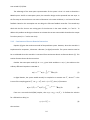
In (1), τ m , with unit Nm, is the torque applied to the gear. It is generated by the servo motor. Given
the torque, it is necessary to convert the torque to a voltage that will be applied to the DC motor. By
analyzing the motor dynamics [1], we have
τm =
η gηm K g K t (Vm − K g K mθ)
Rm
(3)
where η g is gearbox efficiency, η m is motor efficiency, K g is total gearbox ratio, K t is motor torque
constant, K m is back-emf constant, and Vm is motor voltage. Rearrange (3) we get
Vm =
Rm
τ + K g K mθ
η gηm K g K t m
Equation (4) shows that the output voltage depends on the torque τ m and the arm velocity θ .
5-2
(4)
Last revised 07/27/2011
5.1.2
State-Space Representation
Equations (1) and (2) show that the pendulum system is a non-linear system. However, non-linear
systems are difficult to analyze, so we simplify the problem by linearizing the equations and get a
collection of linear equations that approximates of the non-linear equations [1]. Consequently, we can
define a state variable and utilize the state space representation, which is a standard form to describe
multi-in multi-out dynamic system.
The state variable is defined as
θ 
 
α
x= 
 θ 
 
 α 
(5)
where θ is the horizontal arm angle, θ is the horizontal arm velocity, α is the pendulum angle, and α is
the pendulum velocity. Note that the encoders in the pendulum system only get the arm and pendulum
angles. Consequently, only part of the state variable x is known and we will deal with it later.
The state-space representation of the inverted pendulum is

x=Ax+B
u
y=Cx+Du
(6)
where u is the voltage applied to the DC motor. In (6), A is a 4x4 square matrix, B is a 4x1 matrix, C
is a 2x4 matrix, and D is a 2x1 matrix. The analytical solutions to these matrices are
0 0

0 0
=
A 
 0 a32

 0 a42
1
0
a33
a43
0 

1 
=
,B
a34 

a44 
0
 
0
1 0 0 0 
0
=
,C 
=
,D  

 b3 
0 1 0 0
0
 
 b4 
where
5-3
Last revised 07/27/2011
a32 =
m 2p l p2 rg
J arm m p l p2 + J arm J p + m p r 2 J p
a33 = −
a34 =
a42 =
b3 =
( J arm m p l p2 + J arm J p + m p r 2 J p ) Rm
m p l p rB p
J arm m p l p2 + J arm J p + m p r 2 J p
m p l p g ( J arm + m p r 2 )
J arm m p l p2 + J arm J p + m p r 2 J p
a43 = −
a44 =
Barm ( J p + m p l p2 )
m p l p rBarm
( J arm m l + J arm J p + m p r 2 J p ) Rm
2
p p
B p ( J arm + m p r 2 )
J arm m p l p2 + J arm J p + m p r 2 J p
(m p l p2 + J p )
( J arm m p l p2 + J arm J p + m p r 2 J p ) Rm
b4 = −
m pl p r
( J arm m l + J arm J p + m p r 2 J p ) Rm
2
p p
Given the numerical solution to each variable in Appendix A, we can calculate the numerical
solutions to the matrices. The results are
0
1
0 
0


0
0
0
1 

A=
 0 53.1012 −0.6586 0.6575 


 0 98.3814 −0.6575 1.2182 
0




0


B=
 274.4012 


 273.9627 
1 0 0 0 
C=

0 1 0 0
0
D= 
0
5-4
Last revised 07/27/2011
The advantage of the state space representation of the system is that it is easier to describe a
MIMO system. And for a state-space system, the controller design can be separated into two steps. In
the first step we assume that we can access all elements in the state variable x, i.e. we have a full state
feedback. Based on this assumption we can design the full-state feedback controller. The second step
deals with the fact that we are missing part of the elements in the state variable, i.e. θ and α . To
address this problem we design an observer to estimate the current state variable x based on the output
from the system (i.e. θ and α over time).
5.1.3
Continuous to Discrete Domain Conversion
Equation (6) gives the continuous model of the pendulum system. However, when the controller is
implemented on computers, it becomes a discrete (i.e. digital) controller. The system matrices need to
be re-calculated when the controller is converted from continuous domain to discrete domain [2]. This
section discusses how to do the conversion.
Consider the state space model (6). At t = t0 , given initial condition x = x(t0 ) , the solution to the

ordinary differential equation x=Ax+Bu
is
t
=
x(t ) e A (t −t0 ) x(t0 ) + ∫ e A (t −τ ) Bu (τ )dτ
t0
(7)
In digital domain, the system would normally be sampled at a constant rate F , where F is the
inverse of the sampling period Ts . Let t0 = nTs and =
t (n + 1)Ts , then (1.7) becomes
x((n + 1)=
Ts ) e ATs x(nTs ) + ∫
( n +1)Ts
nTs
e A (( n +1)Ts −τ ) Bu (τ )dτ
(8)
If we use a zero-order hold (ZOH) sampler, then u=
(τ ) u=
(t0 ) u (nTs ) . To facilitate the solution
for a ZOH with no delay, let
η =(n + 1)Ts − τ
then we have
5-5
(9)
Last revised 07/27/2011
Ts
x((n + 1)=
Ts ) e ATs x(nTs ) + ∫ e Aη dη Bu (nTs )
0
(10)
In (10), if we define
F = e ATs
Ts
G = ∫ e Aη dηB
0
(11)
H=C
J=D
then we get
x(n +=
1) Fx(n) + Gu (n)
=
y (n) Hx(n) + Ju (n)
(12)
Compare (11) with (6), we can see that (11) is the standard difference equations for a discrete
system.
Using an infinite exponential series expansion, matrix G can be represented as
A k Tsk +1
B
k = 0 ( k + 1)!
∞
G=∑
(13)
Matlab can be used to convert a continuous system to a discrete system using the function c2d() as
shown in Figure 2. The syntax of c2d() is sysd = c2d(sys, Ts, 'method'), where sys is the continuous
system to be discretized, Ts is the sampling period, and 'method' is the discretization method, which is
chosen to be the zero-order hold (zoh) in the project.
% A,B,C,D are constant matrices for pendulum system
% Creates a system
pend=ss(A,B,C,D);
% then discrete the continuous system
pend_d=c2d(pend,Ts,'zoh');
Figure 2 Sample Code to Call c2d()
5.2 Balance Controller Design
Once the physical system has been represented, we must determine the amount of feedback gain
to apply to the system. This section describes how to design the controller to balance the pendulum.
5-6
Last revised 07/27/2011
5.2.1
Full-State Feedback Controller Design
To determine the feedback gain, we first assume a full-state feedback, i.e. all the elements in the
state variable x are known. Based on this assumption, the block diagram is shown in Figure 3.
Plant
u ( n)
x( n)
x(n +=
1) Fx(n) + Gu (n)
Control Law
−K
Figure 3 Block Diagram of the Full-State Feedback Control System
Here we use the linear quadratic regulator (LQR) algorithm to design the state feedback controller.
For a continuous system=
x Ax + Bu , LQR theory states that the full-state feedback control system
satisfies the following criteria [3]
(1) The closed-loop system is asymptotically stable
=
(2) The cost function, defined
as J
∫
∞
0
(xT Qx + u T Ru )dt , is minimized with feedback control law
u = −Kx
where Q is a nonnegative-definite matrix that penalizes the state variable x in the cost function ,
and R is a positive-definite matrix that penalizes the control input u in the cost function. Note that it
follows that the LQR-based control design requires the availability of all the elements in the state
variable x . The feedback control gain K given by
K = R −1BT P
(14)
where P is found by solving the continuous time algebraic Riccait equation
AT P + PA − PBR −1BT P + Q =
0
5-7
(15)
Last revised 07/27/2011
1) Ax(n) + Bu (n) , the cost function J
Similarly, for a discrete linear system described by x(n +=
is
=
J
∞
∑ ( x( k )
T
Qx(k ) + u (k )T Ru (k ))
(16)
k =0
and the feedback gain K can be calculated as [2]
K
= ( R + BT PB) −1 BT PA
(17)
where P is the unique positive definite solution to the discrete time algebraic Riccati equation
P=
Q + AT (P − PB( R + BT PB) −1 BT P ) A
(18)
We can use the Matlab function dlqr() to calculate K . The syntax is [K,S,e] = dlqr(A,B,Q,R), where A
and B is the matrix of discrete-time state-space system model, Q and R are the parameters defined in
the cost function. Sample code is shown in Figure 4. Note that F and G are the same variables used in
(11).
%% Design digital LQR controller
x = 0.2;
%weighting factor for the pendulum position
y = 0.4;
%weighting factor for the pendulum angle
Q = [x 0 0 0;
0 y 0 0;
0 0 0 0;
0 0 0 0];
R = 5;
K_controlgain = dlqr(F,G,Q,R)
Figure 4 Sample Code to Call dlqr()
5.2.2
Observer Design
As indicated above, we do not have direct access to the complete state variable. Consequently, we
must estimate the missing values, which can be done using an observer [3]. The general form of the
state variable feedback compensator is
xˆ = Axˆ + Bu + L(y − Cxˆ )
5-8
(19)
Last revised 07/27/2011
where x̂ denotes the estimate of the state variable x, and L is a matrix representing a collection of
coefficients to be determined.
If we define the estimation error, e, as
e= x − xˆ
(20)
x − xˆ = Ax + Bu − ( Axˆ + Bu + L(y − Cxˆ ))
= A(x − Axˆ ) − L(Cx − Cxˆ )
(21)
and (6)-(19), we get
= ( A − LC)(x − xˆ )
Consequently
=
e ( A − LC)e
(22)
Control theory indicates that if all the poles (i.e. roots) of system (22) locate inside the unit circle,
the system is stable. Therefore, given a vector P of desired, self-conjugate, closed-loop pole locations,
the matrix L can be determined by calling Matlab function place(). The syntax is K = place(A, B, p),
where A and B are the matrices of discrete-time state-space system model, and p is the vector for pole
locations.
In the discrete domain, the observer design is similar. The equation for the observer is
xˆ (n +=
1) Fxˆ (n) + Gu (n) + L(y (n) − Hxˆ (n))
(23)
and the estimation error can be defined as
e=
(n) x(n) − xˆ (n)
(24)
Then (11)-(23) we get
e(n + 1)= xˆ (n + 1) − x(n + 1)
= Fx(n) + Gu (n) − (Fxˆ (n) + Gu (n) + L(y (n) − Cxˆ (n)))
= (F − LH )(x(n) − xˆ (n))
= (F − LH )e(n)
5-9
(25)
Last revised 07/27/2011
We can also call place() to determine the matrix L as shown in Figure 5, where F and H represents
the matrices in (1.11), and F’ represents the transpose of F.
%
P
%
L
pole locations
= [-0.3; -0.3; -0.9; -0.9];
pole placement
= place (F',H',P)';
Figure 5 Sample Code to Call place()
Therefore, the block diagram of the control system based on (23) is shown in Figure 6.
u ( n)
Plant
x( n)
x(n +=
1) Fx(n) + Gu (n)
Control Law
−K
Sensor
y ( n)
H
Observer
xˆ (n)
xˆ (n +=
1) Fxˆ (n) + Gu (n) + L(y (n) − Hxˆ (n))
Figure 6 Block Diagram of the Control System without Reference Signal
5.2.3
Controller with Reference Signal Input
A limitation of the above controller is that it does not accept a “reference input”. In the general
case, a “reference input” is a desired output that the system will converge to. Recall that for the rotary
θ 
inverted pendulum, the output y is   , which has 2 elements. In order to keep the pendulum
α 
balanced, the pendulum angle α should be 0 all the time, so that the only variable that we can control
is the horizontal arm angle θ . In this case, we only set the reference input to a scalar. This section
discusses how to design the controller in the presence of a reference input.
5-10
Last revised 07/27/2011
Let us first repeat the plant (12) and controller equations (23), where the plant refers to the system
being controlled, i.e. the pendulum
x(n +=
1) Fx(n) + Gu (n) 
 plant
y (n) = Hx(n)

(26)
xˆ (n + 1) = (F − GK − LH )xˆ (n) + Ly (n) 
 controller
u (n) = −Kxˆ (n)

(27)
Therefore, if we want to control the horizontal arm angle, the controller receives a reference input
r (n) and (27) becomes
xˆ (n + 1) = (F − GK − LH )xˆ (n) + Ly (n) + Mr (n) 
 controller
u ( n) =
−Kxˆ (n) + Nr (n)

(28)
where M (a matrix) and N (a vector) are to be determined. To determine M and N, the criterion is
that r (n) does not have any influence on the system, which means that the state error,
e=
(n) x(n) − xˆ (n) , is independent of r (n) .
Since
x(n +=
1) Fx(n) + Gu (n)
= Fx(n) + G (−Kxˆ (n) + Nr (n))
=
Fx(n) − GKxˆ (n) + NGr (n)
(29)
xˆ (n + 1) = (F − GK − LH )xˆ (n) + Ly (n) + Mr (n)
=(F − GK − LH )xˆ (n) + LHx(n) + Mr (n)
(30)
x(n + 1) − xˆ (n + 1) = (F − LH )(x(n) − xˆ (n)) + ( NG − M )r (n)
(31)
and
(29)- (30) we get
(n) xˆ (n) − xˆ (n) we get
Substituting e=
e(n + 1) = (F − LH )e(n) + ( NG − M )r (n)
5-11
(32)
Last revised 07/27/2011
In (32), if r (n) has no effect on e(n) , it must be true that NG − M =
0 , therefore
M = NG
(33)
Since G is known, the only thing we need to determine is N , the reference gain. If we assume
that x(n) = xˆ (n) for a sufficient large n, which indicates that the estimated state converges to the real
pendulum state after sufficient long time, then we get
x(n +=
1) Fx(n) + Gu (n)
=
Fx(n) + G ( Nr (n) − Kxˆ (n))
=
Fx(n) + G ( Nr (n) − Kx(n))
=
(F − GK )x(n) + NGr (n)
(34)
Take the z-transform on both sides
zX ( z ) =
(F − GK ) X( z ) + NGR( z )
(35)
Solve X( z ) and get
−1
X( z ) = ( zI − F + GK ) NGR( z )
(36)
Consequently, the z-transform of the output y (n) is
Y( z ) = HX( x)
−1
= H ( zI − F + GK ) NGR ( z )
(37)
If we assume that the reference input is a step signal, which means that r (n) = 1 for n ≥ 0 . For
( z ) z / ( z − 1) , we can apply the final value theorem to (1.36) and
the step signal, the z-transform is R=
get
lim =
y (k ) lim( z − 1)Y( z )
k →∞
z →1
−1
= lim( z − 1)H ( zI − F + GK ) NGz / ( z − 1)
z →1
−1
1
= NH (I − F + GK ) =
G  
0
and we determine the numerical value of the reference gain N from (38) by calculating matrix U
5-12
(38)
Last revised 07/27/2011
−1
U=H (I − F + GK ) G
(39)
and
N=
1
U(1)
(40)
where U(1) represents the first row of matrix U.
Therefore, the resulting control system block diagram with a reference signal is designed in Figure
7.
u ( n)
r ( n)
N
Plant
+
x( n)
x(n +=
1) Fx(n) + Gu (n)
-
Control Law
y ( n)
Sensor
H
Observer
xˆ (n)
xˆ (n +=
1) Fxˆ (n) + Gu (n) + L(y (n) − Hxˆ (n))
−K
Figure 7 Block Diagram of the Control System with Reference Signal
The observer can be implemented based on its state-space representation, which is
ˆ ˆ + Bu
ˆˆ
=
xˆ Ax
ˆ ˆ + Du
ˆˆ
=
yˆ Cx
(41)
where the state variable x̂ is the estimation of x.
Note that in Figure 7, the observer has two inputs: u and y, so define the input for the observer as
u 
uˆ =   , and the other matrices are
y
5-13
Last revised 07/27/2011
1

ˆ =−
ˆ =
0
A
( A LC), Bˆ =
(B L), C
0

0
0 0 0
0


1 0 0 ˆ 0
,D =
0
0 1 0


0 0 1
0
0 0

0 0
0 0

0 0
5.3 Simulation
Section 5.2 gives the theoretical solution to the controller. Based on the control block diagram in
Figure 7, we can implement the control system in Simulink, and simulate the performance of the
controller.
5.3.1
Simulink Simulation Model
The Simulink representation of the complete model is shown in Figure 8, in which each rectangle is
a Simulink block or subsystem. For example, the block “rotary pendulum” fully characterizes the
pendulum system. The State Space Observer subsystem characterizes the Observer. The detail of the
State Space Observer subsystem is shown in Figure 9.
7
theta_ref
1
2
D2R
arm reference Degrees to
position(degrees) Radians
y _d
4
3
-K-
5
6
tau (N.m)
Vi (V)
Vi (V)
RefGain
Vm (V)
th_dot (rad/s)
Select
theta_dot
Actuator Electrical
Dynamics
Torque-Voltage
Actuator Dynamics
y(n)=Cx(n)+Du(n)
x(n+1)=Ax(n)+Bu(n)
y
Scopes
rotary pendulum system
9
8
Y
K*u
Xhat
u
LQR Control Gain
State Space Observer
Figure 8 Simulink Model with Motor Dynamics
5-14
Simulation model for the Quanser rotary inverted pendulum.
Use the State Space Observer to estimate the state.
Last revised 07/27/2011
1
Y
2
y(n)=Cx(n)+Du(n)
x(n+1)=Ax(n)+Bu(n)
u
Vector
Concatenate
K*u
Gain
Discrete State-Space1
1
Xhat
Figure 9 State-Space Observer
5.3.2
Parameters
Parameters that can be adjusted include the sampling period, the Q and R matrices, and the poles’
angles. Configure the system with the following parameters:
•
sampling period Ts=0.001s
•
LQR algorithm matrices Q=[0.2 0 0 0;0 0.4 0 0; 0 0 0 0;0 0 0 0], R = 5
•
Poles are at [-0.3; -0.3; -0.9; -0.9].
Once we have the Simulink model, the controller can be can simulated.
The first experiment tests whether the controller can balance the pendulum. Set the reference
signal to 0, which means that we keep the horizontal arm at a fixed angle of 0 degree. Assume that the
initial state of the pendulum is
 0.1 
 
0.1
x0 =  
 0.5 
 
 0.5 
which means that initially the vertical pendulum and the horizontal arm are at 0.1 rad (5.7 degrees), and
their velocities are 0.5 rad/s. Apparently, the pendulum deviates from the up-right position and is
rotating, so it is not balanced. The controller works at the sampling rate of 1KHz. Figure 10 shows the
arm and pendulum angles changing over time. From the figure, we can see that at t=0, the values of α
5-15
Last revised 07/27/2011
and θ are 5.7. Within 3 seconds, both α and θ converges to 0, which means that the pendulum is
balanced.
Horizontal Arm Position
6
reference position
5
θ
position (degree)
4
3
2
1
0
-1
-2
0
0.5
1
1.5
time (s)
2
2.5
3
Pendulum Position
6
α
5
position (degree)
4
3
2
1
0
-1
-2
0
0.5
1
1.5
time (s)
2
2.5
3
Figure 10 Simulation Result when X0=[0.1;0.1;0.5;0.5]
The second experiment tests whether the horizontal arm angle can follow the reference signal. Set
the reference input to a square wave with an amplitude of 0.1 rad (5.73 degrees), and a frequency of 0.1
Hz. Figure 11 shows the results of the pendulum angle and arm angle. We can see that the arm angle
tracks the reference input and keeps the pendulum angle within 1.5 degrees, which indicates the
pendulum is balanced.
5-16
Last revised 07/27/2011
Horizontal Arm Position
8
6
position (degree)
4
2
0
-2
-4
reference position
α
-6
-8
0
2
4
6
8
10
time (s)
12
14
16
20
18
Pendulum Position
1.5
θ
position (degree)
1
0.5
0
-0.5
-1
-1.5
0
2
4
6
8
10
time (s)
12
14
16
18
20
Figure 11 Pendulum System Simulation Result
5.3.3
Networked Control System Model
To simulate a networked control system, a model was created (Figure 12) using the TrueTime
toolbox [4]. The TrueTime Network block (number 11 in Figure 12) can be configured to be one of
several networks (e.g. Ethernet, CAN), and its bit rate or loss rate.
In Figure 12, subsystems 1-6 are the same as those of the control system in Figure 8 (i.e. the local
control system). But it is divided into two isolated systems: the controller system and the pendulum
system. The pendulum system (blocks 1-4) communicates with the controller (blocks 5,6,8) using the
facilities of the TrueTime send/receive blocks (blocks 7-10).
5-17
Last revised 07/27/2011
3
2
1
4
X_d
tau (N.m)
u
-K-
Vi (V)
Vi (V)
y(n)=Cx(n)+Du(n)
x(n+1)=Ax(n)+Bu(n)
Vm (V)
th_dot (rad/s)
reference signal
RefGain
Actuator Electrical
Dynamics1
Torque-Voltage
Actuator Dynamics
X
Scopes
rotary pendulum system
Data
1: 2
1: 2 Data
Trigger
Sensor
Trigger
TrueTime Receive
(Actuator)
10
TrueTime Send
(Sensor)
7
5
Select
theta_dot
Y
Xhat
6
u
K*u
Data
Data
State Space Observer
1: 3
1: 3
Control gain K
Trigger
Trigger
TrueTime Send
9
1 Schedule
TrueTime Receive
(Controller)
8
Simulate Network Controller for Quanser Inverted Pendulum
Network
Schedule
TrueTime Network
11
Figure 12 NCS Simulink Model
Horizontal Arm Position
8
6
position (degree)
4
2
0
-2
-4
reference position
-6
-8
θ
0
2
4
6
8
10
time (s)
12
14
16
18
20
Pendulum Position
2
α
1.5
position (degree)
1
0.5
0
-0.5
-1
-1.5
-2
0
2
4
6
8
10
time (s)
Figure 13 NCS Simulation Result
5-18
12
14
16
18
20
Last revised 07/27/2011
The pendulum system sends get the angle information and to the controller, where the data rate is
controlled by the sensor trigger. The pendulum receives the control signal and writes it to the actuator.
The controller system receives the angle information, calculates the control signal, and sends it back to
the actuator through controller sender (block 9).
Simulate the network control system using the same parameters listed in 5.3.2, and the simulation
result is shown in Figure 13. Compare Figure 13 and Figure 11, we can see that the maximum pendulum
angle in Figure 13 is 1.5 degrees, which is larger than that in Figure 11. This may be because of the delay
effect in the network.
5.4 Simulink Executable Model
Using Quanser QUARC library, we can compile a Simulink model into a QNX executable image that
can be used to control the actual system. This executable model is implemented in Figure 14. The
structure of the executable model was developed based on the Simulink model shown in Figure 8.
5
theta_ref
y _d
4
2
1
y
D2R
-K-
tau (N.m)
Vm (V)
arm reference
Degrees to
position(degrees)
Radians
Scopes
3
RefGain
X
Y
X
enable
Mode Control
enable
rotary pendulum system
Executable model for the Quanser rotary inverted pendulum.
Use the State Space Observer to estimate the state.
7
6
Y
K*u
Xhat
u
LQR Control Gain
State Space Observer
Figure 14 Executable Simulink Model
Compare Figure 14 with Figure 8, we see that a Mode Control (MC) subsystem is present in Figure
14. The MC receives the output of the pendulum and output an enable signal, which controls when the
balance controller begins to execute. The MC subsystem is necessary because that the encoders only
5-19
Last revised 07/27/2011
give the relative angle, not the absolution angle. This is the limitation of the encoders. When powered
on, the encoders read 0. If the pendulum is at arbitrary position, we cannot tell the exact angle.
However, there is one deterministic position, i.e. when the pendulum is static, it must be in the straight
down position, which is 180 degrees. Therefore, the MC subsystem utilized this information. When the
model begins to execute, the MC subsystem assumes that the pendulum is static, and wait for the user
to swing it up. The controller can only work when the pendulum is close to the up-right position. The
threshold is defined as 2.5 degrees. If the pendulum angle is larger than the threshold, the MC subsystem outputs 0 to disable the controller. Otherwise, the MC subsystem outputs 1 to enable the
controller. The MC subsystem is designed as in Figure 15.
CATCH_ALPHA_UP_LIM
Catching Pendulum Position Limit (rad)
>=
1
|u|
X
Select alpha
|alpha_up|
1
Trigger
Sw Trigger
1
enable
Switch
Trigger Value
Holds states
once enabled
Figure 15 Mode Control Subsystem
The pendulum system sub-system is the one that directly controls the Q4 board and the power
module. Figure 17 shows the details of the subsystem. The HIL initialize block will initialize the Q4 board
when the model begins to execute. The HIL Read Encoder block reads encoder values. The TorqueVoltage Actuator Dynamics and Actuator Electrical Dynamics subsystems convert the input torque to the
desired voltage, which will be output by the HIL Write Analog block to the power amplifier.
5-20
Last revised 07/27/2011
Figure 16 Pendulum System Subsystem
The Calculate Upright Angle subsystem (Figure 17) is used to convert the pendulum angles from its
encoder values. When the pendulum is initially at its straight-down position, the encoder reads 0, which
is mapped to 180 degrees. When the pendulum is swung up, the encoder reads either 2048 or -2048,
which is mapped to 0 degree. This subsystem apply the modulo operation to the input angle, and
subtract the offset angle to get the absolution angle.
1
alpha
mod
2*pi
Mod Angle
(rad)
1
pi
Math
Function Offset Angle
(rad)
alpha_up
Figure 17 Calculate Upright Angle Subsystem
5-21
Last revised 07/27/2011
Figure 18 Running Result
Compile and run the model, we can see that the controller can balance the pendulum. Figure 18
records the arm and pendulum angles during an experiment. The horizontal arm is tracking the input
reference signal, which is a square wave with amplitude of 10 and frequency of 0.1 Hz.
5.5 Summary
This chapter introduces how the pendulum controller is designed. The general process is as follows.
First, analyze the mathematical representation of the physical system. Second, design the control
system block diagram based on control theory. Third, create the Simulink model based on the control
block diagram, and tune the parameters to make sure that the controller is working properly. Forth,
5-22
Last revised 07/27/2011
implement the executable controller by utilizing the Quanser library. In the end, compile and run it on
hardware.
References
[1] Quanser Inc., "Rotary Experiment #08: Self Erecting Inverted Pendulum Control," .
[2] G. Franklin and D. Powell, Digital Control of Dynamic Systems. Addison-Wesley publishing
company, 1980.
[3] R. Dorf and R. Bishop, Modern Control Systems. Prentice Hall, 2008.
[4] Department of Automatic Control, Lund University. TrueTime toolbox. [online]. 2.0 beta 6
Available: http://www.control.lth.se/user/truetime/.
5-23
Last revised 07/27/2011
6
C++ Project
Though Quanser QUARC library and Simulink provides a fast way to construct a controller, the
drawback is that the sampling rate cannot be varied in the Simulink model, because it is a fixed
environment parameter. This restricts the further research on the time scales control theory, which
requires the sampling rate to be altered during runtime. The time scales can be generated by hardware,
i.e. utilizing an external signal generator. However, it is still difficult to directly control the signal
generator in Simulink. Therefore, I created a software solution by implementing the controller in C++.
6.1 C++ Version of the Balance Controller
The C++ version of the pendulum controller is implemented by mimicking the Simulink model. The
C++ code implements all the functions that are in the executable Simulink model. The executable
Simulink model is redrawn in Figure 1, in which subsystems that pertain to the same functional group
are circled in red circle.
The reference signal group generates a proper reference signal, and applies the correct gain to
eliminate the steady-state error. The controller group determines the status of the pendulum, uses the
observer to estimate the current state variable, and applies the LQR feedback control law. The Q4 board
group directly accesses the Q4 board to read/write data.
The C++ program can be modeled using SysML. The Block Definition Diagram (BDD) describes the
general structure of the system. The BDD of the pendulum system is shown in Figure 2. The
PendulumSystem class is the top-level class that is composed of three main classes: Reference Signal,
Controller, and Q4. The PendulumSystem class stores the state variable and other variables that are
exchanged between different classes and are frequently updated. The reason is that the difference
equation x(n +=
1) Fx(n) + Gu (n) indicates that the next pendulum state variable x(n + 1) is
6-1
Last revised 07/27/2011
calculated based on the current input u (n) , and the current state variable x(n) , which should be
saved. Therefore, I designed the PendulumSystem class to be the top class that keeps track of
everything.
5
Q4 board
theta_ref
y _d
4
2
1
y
D2R
-K-
tau (N.m)
Vm (V)
arm reference
Degrees to
position(degrees)
Radians
Scopes
3
RefGain
X
Y
X
enable
Reference
Mode Control
enable
rotary pendulum system
Executable model for the Quanser rotary inverted pendulum.
Use the State Space Observer to estimate the state.
7
6
Y
K*u
Xhat
u
LQR Control Gain
State Space Observer
Controller
Figure 1 Executable Simulink Model
The internal structure is best described using the Internal Block Diagram (IBD). The advantage of
SysML is that we can show the interfaces and data flow between each subsystem. As shown in Figure 3,
the Reference Signal class outputs angle data (i.e. the horizontal arm position) to the Controller block.
The Q4 block outputs encoder data (in the form of a Matrix) to the Controller block. Based on these
information, the Controller calculates the voltage to be applied to the DC motor, and outputs it to the
Q4 block.
6-2
Last revised 07/27/2011
Figure 2 BDD of pendulum system
Figure 3 IBD of PendulumSystem block
6-3
Last revised 07/27/2011
6.2 Varying Sampling Rate
Varying sampling rate is achieved by using a QNX software timer. The QNX provides software timers
whose expiration time could be set during runtime. At each timer expiration, the QNX OS sends a signal
to the C++ grogram, which is waiting for that signal. Upon receiving the signal, the main() function will
call the update() function in the PendulumSystem class, which reads encoder data, calculates the control
signal (voltage), and outputs the voltage to the Q4 class.
The PendulumSystem::update() function accepts an input parameter of Boolean type, which
indicates whether the controller runs at a fixed rate or a variable rate. The return value indicates what
the next sampling period is (Figure 5), so the software time can be set. In this way, the timer expiration
time it set at each step so that the sampling rate is varying. This gives us the flexibility to generate time
scales.
The implementation of the PendulumSystem::update() function is shown in Figure 4. If the fixed
step length flag is to false, the function calculates the Euclidian norm of the current estimated state
variable x̂ , then determine the next sampling period based on that norm.
//if using time scales control, determine next sampling
period
if(!isFixedRate)
{
//calculate norm of the vector
double dp = matrix_Xhat_.norm();
int index = 0;
if(dp > 2)
{
nextTs = constants::TS5MS;
}
else
{
nextTs = constants::TS20MS;
index = 1;
}
controller.loadParameters(index);
refpos.loadParameters(index);
}
Figure 4 int PendulumSystem::update(bool isFixedRate)
6-4
Last revised 07/27/2011
int Ts = mysys.update(true);
//set timer
//expire time = Ts
itime.it_value.tv_sec = 0;
itime.it_value.tv_nsec = Ts;
//reload time = Ts
itime.it_interval.tv_sec = 0;
itime.it_interval.tv_nsec = Ts;
timer_settime(timer_id, 0, &itime, NULL);
Figure 5 Calling PendulumSystem::update()
6-5
Last revised 07/27/2011
7
Creating your own controller
When you need to create your own controller, you can modify the existing Simulink and QNX C++
project.
7.1 Step 1
The first step is to create a simulation model in Simulink. This requires you to modify file
sim_statespace_obeserver.mdl, as shown in Figure 1.
7
theta_ref
1
2
D2R
arm reference Degrees to
position(degrees) Radians
4
3
-K-
y _d
5
6
tau (N.m)
Vi (V)
Vi (V)
RefGain
y(n)=Cx(n)+Du(n)
x(n+1)=Ax(n)+Bu(n)
Vm (V)
th_dot (rad/s)
Select
theta_dot
Actuator Electrical
Dynamics
Torque-Voltage
Actuator Dynamics
y
Scopes
rotary pendulum system
9
8
Y
K*u
Xhat
u
LQR Control Gain
State Space Observer
Simulation model for the Quanser rotary inverted pendulum.
Use the State Space Observer to estimate the state.
Figure 1 sim_statespace_obeserver.mdl
You should keep block 1, 4, 5 and 6. Block 1 generates and outputs the reference angle. Block 4 and
5 are for motor dynamics, which converts the torque to voltage. Block 6 is the physical model of the
pendulum system, which accepts voltage and outputs the arm and pendulum angles.
Then create your own controller by adding the controller blocks into the diagram.
7.2 Step 2
After you get successful simulation results, you can modify file exe_statespace_obeserver.mdl.
7-1
Last revised 07/27/2011
5
theta_ref
y _d
4
2
1
y
D2R
-K-
tau (N.m)
Vm (V)
arm reference
Degrees to
position(degrees)
Radians
Scopes
3
RefGain
X
Y
X
enable
Mode Control
enable
rotary pendulum system
Executable model for the Quanser rotary inverted pendulum.
Use the State Space Observer to estimate the state.
7
6
Y
K*u
Xhat
u
LQR Control Gain
State Space Observer
Figure 2 exe_statespace_obeserver.mdl
Block 1, subsystem 3, and subsystem 4 should be kept. Block 1 is for reference position generation.
Subsystem 3 determines whether the pendulum can be controlled by the controller. Subsystem 4
contains the Q4 board accessing blocks, which read encoder values and write controls signal to the
pendulum system.
7.3 Step 3
To design new controller for the QNX C++ project, users need to replace the existing Controller
class. Q4 class and Reference class should be kept.
7-2
Last revised 07/27/2011
8 Conclusion
This chapter gives some experiment observations plus conclusion and possible future work.
8.1 Observations
Chapter 5 has illustrated both the simulation and execution experiments results where the
pendulum is balanced. For the controller, many parameters could be tuned. Therefore, this section gives
more experiment result and analyzes the observations.
8.1.1
Comparison of Results
The test bed provides simulation models for the local control system, the networked control system,
and the switched system. Each system has some parameters that can be tuned. Section 8.1.1.1 shows
the observations of tuning the sampling rate for local control system. Section 8.1.1.2 shows the
observations of tuning the sampling rate, packet loss rate, and network type for the NCS. Section 8.1.1.3
shows the observations of tuning the switching threshold for the switched system.
8.1.1.1 Local Control Simulation
The sampling rate is an important parameter. Generally, a control system has a maximum sampling
period (µmax), or minimal sampling rate. Intuitively, a controller cannot work too slowly to control the
inverted pendulum. To determine µmax by simulation, we did several experiments where Ts was set to 5
ms, 40 ms, 20 ms, and 10 ms. The system’s stability is shown in Figure 1. Since the pendulum is still
stable when Ts = 10 ms (Figure 2), but is unstable when Ts = 20 ms (Figure 3). Therefore, µmax must be in
the range of 10 ms to 20 ms.
8.1.1.2 Networked Control Simulation
For an NCS, we can compare the sampling rate, the packet loss rate, and the performance of
different network.
8-1
Last revised 07/27/2011
The first experiment is on the sampling rate of NCS. Assume that the network type is Ethernet with
a data rate of 100 Mbps and no packet loss. When Ts = 5 ms, the simulation results is shown in Figure 4,
in which the oscillation indicates that the LQR controller designed in Chapter 5 cannot balance the
pendulum. When Ts = 4 ms, the simulation results is shown in Figure 5, which shows that the pendulum
is balanced. However, compared to the pendulum angle Figure 2, which is a local control, the pendulum
angle is not as smooth. And comparing the maximum pendulum angle of the two figures, we can see
that the NCS is more than 2 degrees, which is larger than the pendulum angle with the local control.
Therefore, this result shows that an NCS requires a higher sampling rate than a corresponding local
control system.
Ts
5 ms
10 ms
20 ms
40 ms
Stability
Stable
Stable
Unstable
Unstable
Figure 1 Stability against Sampling Period
Horizontal Arm Position
8
reference position
θ
6
position (degree)
4
2
0
-2
-4
-6
-8
0
2
4
6
8
10
time (s)
12
14
16
18
20
Pendulum Position
2
α
1.5
position (degree)
1
0.5
0
-0.5
-1
-1.5
-2
0
2
4
6
8
10
time (s)
12
14
Figure 2 Local Control (Ts = 10 ms)
8-2
16
18
20
Last revised 07/27/2011
88
2
Horizontal Arm Position
x 10
0
position (degree)
-2
-4
-6
-8
reference position
-10
-12
θ
2
0
4
6
8
89
0.5
10
time (s)
12
14
16
18
20
Pendulum Position
x 10
α
-0.5
-1
-1.5
-2
-2.5
0
2
4
6
8
10
time (s)
12
14
16
18
20
Figure 3 Local Control (Ts = 20 ms)
Horizontal Arm Position
100
reference position
θ
position (degree)
50
0
-50
-100
0
2
4
6
8
10
time (s)
12
14
16
18
20
Pendulum Position
100
α
50
position (degree)
position (degree)
0
0
-50
-100
0
2
4
6
8
10
time (s)
12
14
16
18
Figure 4 Network Control (Ethernet, 100Mbps, Ts = 5 ms, loss rate = 0)
8-3
20
Last revised 07/27/2011
Horizontal Arm Position
10
position (degree)
5
0
-5
reference position
-10
θ
0
2
4
6
8
10
time (s)
12
14
16
18
20
Pendulum Position
3
α
position (degree)
2
1
0
-1
-2
-3
0
2
4
6
8
10
time (s)
12
14
16
18
20
Figure 5 Network Control (Ethernet, 100Mbps, Ts = 4 ms, loss rate = 0)
Horizontal Arm Position
10
position (degree)
5
0
-5
reference position
θ
-10
0
2
4
6
8
10
time (s)
12
14
16
20
18
Pendulum Position
3
α
position (degree)
2
1
0
-1
-2
0
2
4
6
8
10
time (s)
12
14
16
Figure 6 NCS (Ethernet, 100Mbps, Ts = 2 ms, loss rate = 2%)
8-4
18
20
Last revised 07/27/2011
TrueTime toolbox provides the ability to adjust the network parameters. The following experiments
are on other network parameters. For example, we can set the packet loss rate for a TrueTime network.
Still assume that the network type is Ethernet with a data rate of 100Mbps. The sensor data is
transmitted to the controller every 2 ms. When the packet loss rate is 2%, the simulation result is shown
in Figure 6. We can see that the pendulum angle has some random pattern compared to Figure 2 Local
Control (Ts = 10 ms). This is because some packets are lost during the transmission, so that the
controller cannot calculate a correct control signal. In this case, the pendulum may become unstable.
We can also set the network type. For example, assume the network type is CAN with a data rate of
1 Mbps and no packet loss. Figure 7 shows the simulation result when Ts = 4 ms. Though CAN has a
much slower transmission rate (1Mpbs) than Ethernet (100Mbps), the pendulum is still balanced. This is
because that CAN bus is very suitable for real time communications systems.
Horizontal Arm Position
10
reference position
θ
position (degree)
5
0
-5
-10
0
2
4
6
8
10
time (s)
12
14
16
18
20
Pendulum Position
3
α
position (degree)
2
1
0
-1
-2
-3
0
2
4
6
8
10
time (s)
12
14
16
Figure 7 NCS (CAN, 1Mbps, Ts = 4 ms, loss rate = 0)
8-5
18
20
Last revised 07/27/2011
8.1.1.3 Switched System Simulation
One of our objectives has been to investigate a stability of the time scales control system, where
the maximum sampling period (µmax) determines the Hilger circle (with radius 1/ µmax) on the complex
plane, inside which the control system stays stable. Even though the system not guaranteed to be stable
outside the Hilger circle, there is a conjecture that as long as the system does not stay outside the Hilger
circle “too long”, the system will remain stable. It should be possible to investigate this controller using
the test bed, where the system would switch from inside to outside of the Hilger circle, and vice versa.
The matlab file sim_switched_system.m simulates the above idea (see in section 5.1 in Appendix C).
The switching threshold is based on the norm of the difference between the pendulum angle and the
reference angle, i.e., || ref − x || , where || x || denotes the Euclidean norm of the vector x. If the
difference is less than the threshold, the controller will work at a longer sampling period (20 ms),
otherwise it will work at a shorter sampling period (5 ms). For example, we set the switching threshold
5ms if || ref − x ||> 0.04
and the arm follows the reference signal of a square with
20ms if || ref − x ||≤ 0.04
to 0.04, i.e. Ts = 
a frequency of 0.1 Hz and an amplitude of 0.1 rad. The results are shown in Figure 8. When the
reference signal changes, the controller works at a shorter sampling period, and when the reference
signal is stable, the pendulum tends to work at a longer sampling period. Figure 9 shows the
experimental results with a threshold 0.1, where the pendulum is still stable. However, the arm angle is
less smooth compared to the arm angle in Figure 9. Therefore, this threshold controls how long the
controller stays inside/outside the Hilger circle. If the threshold is too large, the pendulum may stay
outside the Hilger circle too long and eventually fall.
8-6
Last revised 07/27/2011
positions
0.15
0.1
positions(rad)
0.05
0
-0.05
-0.1
arm position
pendulum position
-0.15
-0.2
0
2
4
6
8
10
12
14
8
10
12
14
10
12
14
10
12
14
Time (s)
Sampling period(µ)
0.02
0.018
0.016
0.014
µ(ms)
0.012
0.01
0.008
0.006
0.004
0.002
0
0
2
4
6
Time (s)
Figure 8 Switched System (threshold = 0.04)
positions
0.15
0.1
positions(rad)
0.05
0
-0.05
-0.1
arm position
pendulum position
-0.15
-0.2
0
2
4
8
6
Time (s)
Sampling period(µ)
0.02
µ(ms)
0.015
0.01
0.005
0
0
2
4
8
6
Time (s)
Figure 9 Switched system (threshold = 0.1)
8-7
Last revised 07/27/2011
8.1.2
Accuracy of Simulations
By comparing Fig. 11 and Fig. 19 in Chapter 4, we can see that the result is different. The simulation
shows a smooth plot and no jitter, which is unlike the real experiments result. The following section
discusses the potential reasons.
8.1.2.1 Mathematical Model Limitation
First, the mathematical model in equation (1) and (2) in Chapter 5 may not be accurate. The
performance of the controller depends on the accuracy of the non-linear model, because the starting
point of the controller design is to model the mathematical system model and get the non-linear
equations of motion. The more accurate the physical model is, the more accurate the pendulum is.
Besides, the controller is designed based on the state space representation of the system. It undergoes
the linear approximation process of the non-linear model. With loss of information, this process also
reduces the accuracy.
8.1.2.2 Motor Model
Second, the motor model also has limitations. SRV-02 incorporates a Faulhaber 2338S006 Coreless
DC Motor with dynamic model shown in equation (4) in Chapter 5. The motor parameters can be found
in the data sheet [1]. However, different motors could have slightly different parameters. Besides, the
motor has a minimal input voltage, which means that the motor only rotates when the input is larger
than this threshold. In Simulation, the horizontal arm moves whatever the input voltage is. Due to this
reason, once the pendulum is near balanced position in real experiment, controller only outputs a small
voltage in which case the arm will not move. After a few cycles, the pendulum will not reach the desired
position. In this case, a large voltage will be generated and it pushes the arm to deviate from the
balanced position.
8-8
Last revised 07/27/2011
8.1.2.3 Finite Wordlength Effect
Another reason could be the finite wordlength effect. The pendulum system uses encoders to get
angle information. With a resolution of 4096, each encoder works as a 14-bit A/D converter, so that
there is a certain amount of uncertainty introduced during quantization. From digital signal processing
theory, we know that this will cause the finite wordlength effect, which means that some information is
lost. On the contrary, Simulink simulation uses double precision variables, so that no angle information
is lost. The finite wordlength effect could be analyzed using the DSP theory [2]. The simulation models
can be improved to consider the finite wordlength effect.
8.1.3
Timing Inaccuracy
The C++ project uses software time to realize varying timer interrupt. Though QNX provides higher
timing accuracy than Windows XP, it still has some jitter and latency. Figure 1 shows the kernel event
tracing of the C++ program captured by QNX Momentics IDE. The vertical line records the time that the
thread receives a message from the timer interrupt. From the figure we can see that the interval
between two messages is actually 6.998 ms, not 5 ms which is preset. Besides, the interval is not fixed,
ranging from 6.997 ms to 7.002ms, which indicates the jitter of the software timer.
Figure 10 Kernal Event Tracing
Hardware (signal generator) provides the most accuracy timing. But currently we cannot directly
control the signal generator in Simulink environment. Therefore future research could investigate how
to improve the hardware to make it controllable.
8-9
Last revised 07/27/2011
8.1.4
Stability against Sampling Rate
Another experiment we did is to check the controller’s stability against different sampling rate. The
result shows that the controller which uses the state-space observer can balance the pendulum over a
large range of sampling rate.
To generate various sampling frequencies, we use the external signal generator. The controller was
designed at the sampling rate of 200 Hz. Follow Appendix C section 5.2 and configure the system to use
the external signal generator. Run the controller. When the pendulum is balanced, adjust the output
frequency of the signal generator. The observation is that if the frequency increased or decreased too
much, the pendulum will unstable. By tuning the frequency, we find that the system is stable within 140
Hz to 240Hz. Figure 11 and Figure 12 show the arm and pendulum angles when sampling rate is 200 Hz
and 240 Hz respectively. From Figure 12, we can see a larger swing of the arm, which indicates instability.
The Qanser Lab 8 (Appendix C Section 2) provides a different observer. It utilizes a differentiator
and a low pass filter to estimate the velocity, which means that the observer calculates the velocity base
on equation v(n) = ( s (n) − s (n − 1)) / Ts , then process v(n) using a low pass filter. By repeating the
above experiment, it is shown that this observer has a larger range of stability, which is 140 Hz to 300 Hz.
Figure 13 and Figure 14 show the arm and pendulum angles when sampling rate is 200 Hz and 300 Hz
respectively. The difference between these two models is due to the different structures. The Quanser
Lab 8 provides a PD controller, while our controller is a LQR controller.
8-10
Last revised 07/27/2011
Figure 11 Running Results (Fs = 200 Hz)
Figure 12 Running Results (Fs = 240 Hz)
8-11
Last revised 07/27/2011
Figure 13 Quanser Lab 8 Running Result (Fs=200Hz)
Figure 14 Quanser Lab 8 Running Result (Fs=300Hz)
8-12
Last revised 07/27/2011
8.2 Conclusions and Future Work
8.2.1
Abilities of The Test Bed
The test bed developed in this project, including the simulator and controller, could help users
understand control systems. The experiments that we have done using the test bed have shown its
ability to test time scales control and network control theories. More importantly, the models in the test
bed provide useful blocks with interfaces that can be reused, so that uses could embed their own
controllers, which is helpful for future researches.
In conclusion, the test bed developed in this project can help facilitate the future research of
developing and verifying the time scales control theory as well as network control theory.
8.2.2
Limitations
Some restrictions have limited the experiments that we can do using this test bed. First, we lack the
time scales control theory for a non-fullstate feedback system. For the pendulum system, where the arm
and pendulum velocities are not directly sensed by sensors, it is not a full-state feedback system. The
traditional pole-placement algorithm does not work quite well in this case. Second, current hardware
configuration cannot send senor data directly to controller, so we have not implemented a real NCS yet.
8.2.3
Future Work
Future research could involve the following areas.
•
Embed velocity sensors in the pendulum system, Add velocity sensors to get the arm and
pendulum velocity, so that we can get complete state variable, and make the system a fullstate feedback system.
•
Develop the time scales observer. If we keep the current hardware configuration, which is
not a full-state feedback system, a time scales observer is needed if we want to use the
time scales control.
8-13
Last revised 07/27/2011
•
Use wireless transmitters to directly transmit sensor data and control signal between the
plant and the controller, which implements an NCS.
•
Apply the time scales theory on NCS. One NCS co-design method is adaptive sampling
period selection, which means that the controller chooses proper sampling period based on
current network condition [3][4]. It has been proved that the adaptive sampling rate is
feasible [4].
References
[1] Quanser Inc., "SRV02 user manual," .
[2] B. Liu, "Effect of finite word length on the accuracy of digital filters--a review," IEEE Transactions
on Circuit Theory, vol. 18, pp. 670-677, 1971.
[3] F. Xia, L. Ma, C. Peng, Y. Sun and J. Dong, "Cross-Layer Adaptive Feedback Scheduling of Wireless
Control Systems," Sensors, vol. 8, pp. 4265-4281, 2008.
[4] I. A. Gravagne, J. M. Davis, J. J. Dacunha and R. J. Marks, "Bandwidth reduction for controller
area networks using adaptive sampling," in Proceedings of the 2004 IEEE International Conference on
Robotics and Automation, New Orleans, LA, 2004, pp. 5250-5255.
8-14
Last revised 07/25/2011
Appendix A
Parameter Definition
The parameters used in Matlab programs are listed in the following table.
Symbol
𝛼
𝛼̇
𝛼̈
𝜃
𝜃̇
𝜃̈
𝑚𝑝
𝑙𝑝
𝑟
𝐽𝑎𝑟𝑚
𝐽𝑝
𝐵𝑎𝑟𝑚
𝐵𝑝
𝑔
𝜂𝑔
𝜂𝑚
𝐾𝑡
𝐾𝑚
𝐾𝑔
𝑅𝑚
𝐼𝑚
𝜏𝑚
Description
Pendulum angle
Pendulum speed
Pendulum acceleration
Arm angle
Arm speed
Arm acceleration
Pendulum Mass with T-fitting
Distance from Pivot to Centre
Of Gravity
Full Length of the pendulum
Moment of inertia acting seen
from arm pivot
Moment of inertia acting seen
from pendulum pivot
Equivalent Viscous Damping
Coefficient
Equivalent Viscous Damping
Coefficient
Standard gravity
Gearbox efficiency
Motor efficiency
Motor torque constant
Back-emf constant
Total gearbox ratio
Motor armature resistance
Motor current
The torque applied at the load
gear
A-1
Matlab Variable
Value(SI units)
mp
lp
0.127Kg
0.1556m
r
Jarm
0.2159m
0.0020
Jp
0.0043
Barm
Bp
0.0024 𝑁𝑚𝑠/𝑟𝑎𝑑
g
eta_g
eta_m
Kt
Km
Kg
Rm
9.81 𝑚/𝑠 2
0.9
0.69
7.68E-3 𝑁𝑚
7.68E-3 𝑉/(𝑟𝑎𝑑/𝑠)
70
2.6Ω
0.0024 𝑁𝑚𝑠/𝑟𝑎𝑑
Last revise 07/26/2011
Appendix B
List of Hardware and Software
The hardware and software used in this project are listed in the following tables.
Hardware
Abbreviation
Q4
Q4 terminal board
UPM-1503
SRV02-E
DI-604
33220A
Name
Data acquisition board
Q4 terminal board
Power module
Servo plant
Router
Signal Generator
Vender
Quanser Inc.
Quanser Inc.
Quanser Inc.
Quanser Inc.
D-Link
Agilent
Technologies
Website
http://quanser.com
http://quanser.com
http://quanser.com
http://quanser.com
http://d-link.com/default.aspx
http://www.home.agilent.com/agilen
t/home.jspx?lc=eng&cc=US
Software
Name
Matlab
QUARC
Momentics IDE
QNX Neutrino RTOS
VMware Player
Agilent IO Libraries
Suite
IntuiLink Waveform
Editor
Vender
The Mathworks, Inc.
Quanser Inc.
QNX software Systems
QNX software Systems
WMware, Inc.
Agilent Technologies
Version
R2010a
2.1
4.7
NA
3.1.3
16.1
Website
http://www.mathworks.com
http://quanser.com
http://www.qnx.com
http://www.qnx.com
http://www.vmware.com
http://www.agilent.com
Agilent Technologies
1.6
http://www.agilent.com
B-1
Last revised 07/27/2011
Appendix C
Test Bed User Manual
1
Set Up the System
1.1 Install Software
Here we assume that the Host runs Windows 7, and the Target runs QNX. Software installed on the
Host includes Matlab, VMware player, the QUARC library and QNX Momentics IDE. On the target, the
QUARC library is installed.
Because the QUARC library does not support Windows 7, we have to install a VMware Player on the
Host so that we could run a virtual Windows XP computer, on which the QUARC library is also installed.
When the QUARC library supports Windows 7, then VMware will not be necessary.
1.2 Connect Wires
The Host and Target computers communicate through an Ethernet connection. They are connected
to a router, and they both obtain their respective IP addresses via DHCP. However, once the IP address
of the Target is defined, this address must be manually in set in the Simulink model (see section 3.4).
The connections among the hardware components are shown in Figure 1.
•
The analog output channel 0 on the Q4 terminal board (port 1) transmits DC motor control
signal, and is routed to the UPM “from D/A” port (port 2).
•
The UPM “to load” port (port 3) emits enough current to drive the DC motor, and is first
connected to a pushdown break button, which in turn is routed to the DC motor port on SRV02
(port 4). The break button, in a blue box with a red button, is used as an emergency stop.
C-1
Last revised 07/27/2011
Normally the switch is closed. In case of emergency (e.g., pendulum rotating wildly), you can
push and hold the red button to temporarily cut off electricity to stop the motor, then turn off
the UPM.
•
The arm encoder on SRV02 (port 6) is connected to the encoder input channel 0 (port 5) on the
Q4 terminal board.
•
The pendulum encoder (port 8) is connected to the encoder input channel 1 (port 7) on the Q4
terminal board.
Figure 1 Wiring Diagram
1.3 Use Source Code Repository
We have used a Subversion repository to manage the files associated with this project, in
conjunction with the QNX Momentics IDE. The repository contains several Matlab/Simulink simulation
files, an executable Simulink model and a QNX C++ project. We can use Eclipse IDE or the QNX
Momentics IDE (which is also Eclipse-based ) to access the repository.
C-2
Last revised 07/27/2011
To access these files for the first time (assuming that the repository has already been created on
the server), follow these steps:
(1) Create a new Eclipse workspace or use an existing workspace.
(2) Define a new repository locations within the IDE as
svn+ssh://[email protected]/home/grad/group/qnx/repository
and provide your user name and password to access the repository.
(3) Once connected, you should see the repository structure similar to Figure 2.
•
The controller folder contains the Simulink project and the C++ project.
•
The documents folder contains reports created in the project.
•
The projectReport folder contains all the project reports.
•
The weeklyReports folder contains Chengsen Song’s weekly reports since July 2010.
C-3
Last revised 07/27/2011
Figure 2 SVN Repository
(4) Navigate and highlight the controller->trunk->controller folder to check out the controller. Right
click the mouse then select check out. Other folder can be similarly checked out.
2
Run the Quanser Example (Lab 8)
Quanser provides an example (Lab 8) to demonstrate how to balance then pendulum. This section
introduces how to run this Quanser example. Before running the Quanser Lab 8, log on the Host and the
Target. Since the Host runs Windows 7 computer, use your user name assign by the administrator,e.g.
ece01\song. For the QNX computer, log in as the super user, with the password quarc_target. Note that
the keyboard is shared between the host and target computers. To use the keyboard on either
computer, hit the “Scroll Lock” key twice to toggle between the computers.
C-4
Last revised 07/27/2011
After logging on both Host and Target, follow these steps:
(1) On the Host (running Windows 7), double click the VMware Player desktop icon to display the
VMware Player window. Then Choose open a virtual machine. You can find the virtual Windows
XP Professional located in C:\VM\XP_PRO. Then select poweron this virtual machine.
(2) On the Target, run Launch->QUARC->Console. An empty console should then appear.
(3) On the Host, switch to the Windows XP virtual machine.
(4) Start Matlab on the Windows XP virtual machine. Change the current working directory to
C:\Mprojects\MATLAB\SRV02 Lab Files\Exp08 - Inverted Pendulum\Lab Files\.
To do this, click the button in the circle shown in Figure 6. Then in the popup dialogue, find the
respective folder and you should see a list similar to Figure 3.
Figure 3 File structure for Quanser lab 8
(5) Open SETUP_SRV02_EXP08_SIP.m, which is a Matlab file used to calculate the pendulum’s
physical parameters and construct a PD controller for the pendulum. Run this file, and the
following results should appear in the Matlab command window:
C-5
Last revised 07/27/2011
SRV02 model parameters:
K
= 1.76 rad/s/V
tau = 0.0285 s
SRV02+SIP
k(1) =
k(2) =
k(3) =
k(4) =
balance control gains:
-0.31623 N.m/rad
1.9146 N.m/rad
-0.14956 N.m/(rad/s)
0.26268 N.m/(rad/s)
Here K represents steady-state gain, tau represents time constants, and k represents the feedback
gain of the PD controller.
(6) Open q_sesip_q4.mdl (where sip stands for “single inverted pendulum”), which contains the
Simulink model, as shown in Figure 4.
Figure 4 q_sesip_q4.mdl
(7) Build the Simulink model by selecting QuaRC->build within the Simulink window.
During the build process, the graphical representation of the Simulink model is translated into C
code. The Target Language Compiler then compiles the C code and generates an executable
binary specific to QNX, which is afterwards downloaded to the target.
(8) Turn on the UPM power module. The switch is on the back towards the top.
(9) Run the program on the Target. In the Simulink model window on the Host, select QuaRC->start.
The controller will cause the pendulum to swing up and then balance the pendulum.
C-6
Last revised 07/27/2011
(10)
Stop the program. In the Simulink model window on the Host, select QuaRC->stop.
(11)
When finished, power off the power amplifier, the Windows XP virtual machine, and the
QNX machine.
3
Run Our Simulink Model
We create our own Simulink model of the pendulum system, which can be used to simulate the
system or actually control the inverted pendulum (when it is near the vertical position). This model can
be used as the basis for designing and fine-tuning other controllers.
3.1 Introduction
The models are located in the following address which should be stored in your personal workspace
: YOUR_WORKSPACE_LOCATION\controller\simulink\quanser_pendulum_control.
The Simulink simulation model uses the LQR algorithm to control the pendulum. It is a different
controller from the PD controller in Quanser Lab 8. The executable Simulink model uses the same LQR
controller, which has several new blocks to directly access the hardware and handle the data.
Run the simulation model following section 3.2, which will display the pendulum and arm positions
in “scopes” to indicate whether the pendulum is balanced. Note that some parameters can be tuned.
You can try to tune these parameters until the results show that the pendulum can be balanced.
After the simulation results become acceptable, you can run the executable model to actually
control the system. This model is compiled, and the binary code can be downloaded and run on the QNX
target machine.
The relevant files are:
C-7
Last revised 07/27/2011
Figure 5 Files contained in the quanser_pendulum_control folder
The setup*.m files are Matlab files used for calculating the pendulum’s physical parameters,
determining control gains and other parameters that are used by the controller. The setup.m file is the
main setup file, which calls the other setup_*.m files.
The .mdl files are Simulink models which can be used to simulate the system. See section 3.3 for
how these files should be used.
After a simulation, the postscript*.m files can be used for drawing figures of the simulation results.
The exe*.mdl files can be compiled, downloaded, and executed on the QNX computer.
3.2 Run the Local Control Model
To run the simulation, follow these steps:
(1) Start Matlab and navigate to the current working directory. To do this, click the button in the
circle shown in Figure 6. Then in the popup dialogue, navigate to :
YOUR_WORKSPACE_LOCATION\controller\simulink\quanser_pendulum_control.
C-8
Last revised 07/27/2011
Figure 6 Change current working directory
(2) Choose File->Open to open the setup.m file. This file first calculates the pendulum’s physical
system parameters, then creates an LQR controller and the state-space observer.
You can adjust several variables to design the controller, including:
•
The sampling period, which controls how fast the controller samples the system
%% sampling period
Ts=0.005;
•
The Q and R matrices for the LQR algorithm
%% Design digital LQR controller
x = 0.2;
%weighting factor for the cart position
y = 0.4;
%weighting factor for the pendulum angle
Q = [x 0 0 0;
0 y 0 0;
0 0 0 0;
0 0 0 0];
R = 5;
K_controlgain = dlqr(F,G,Q,R)
•
The pole locations for the pole-placement algorithm
P = [-0.3 -0.3 -0.9 -0.9];
L = place (F',H',P)';
(3) Click the button in the red circle (or hit F5) to run the setup.m file. This will calculate the
constants and matrices representing the pendulum system. The Matlab command window will
then show the control gain matrices.
Figure 7 Run setup.m
(4) Open the sim_statespace_obeserver.mdl fiel, which represents the entire simulation model
including the feedback controller, observer, and reference signal.
C-9
Last revised 07/27/2011
7
theta_ref
1
2
D2R
arm reference Degrees to
position(degrees) Radians
4
3
-K-
y _d
5
6
tau (N.m)
Vi (V)
Vi (V)
RefGain
Vm (V)
th_dot (rad/s)
Select
theta_dot
Actuator Electrical
Dynamics
Torque-Voltage
Actuator Dynamics
y(n)=Cx(n)+Du(n)
x(n+1)=Ax(n)+Bu(n)
y
Scopes
rotary pendulum system
9
8
Y
K*u
Xhat
u
LQR Control Gain
State Space Observer
Simulation model for the Quanser rotary inverted pendulum.
Use the State Space Observer to estimate the state.
Figure 8 Simulink Simulation Model
(5) Run the model. When finished, you can see the simulation results via the Scopes. To do this,
double click the Scopes subsystem. The details of this subsystem are shown in a new window,
which contains two scopes. In the new window, double click both scopes to see the results.
(6) Because the output is displayed in two scopes, it is difficult to compare and analyze. We can
display the results in a single figure by running the postscript_local.m file, which creates the
diagram in Figure 9.
C-10
Last revised 07/27/2011
Horizontal Arm Position
8
reference position
θ
6
position (degree)
4
2
0
-2
-4
-6
-8
0
2
4
6
8
10
time (s)
12
14
16
18
20
Pendulum Position
1.5
α
position (degree)
1
0.5
0
-0.5
-1
-1.5
0
2
4
6
8
10
time (s)
12
14
16
18
20
Figure 9 Local Control Simulation Result
3.3 Run the NCS Model
We created a network control system (NCS) simulation model by using the TrueTime toolbox to
simulate the network. Before you run the simulation, you must first set up the TrueTime environment.
(1) Start Matlab and switch the current working directory to the following directory located in your
workspace
YOUR_WORKSPACE_LOCATION \controller\simulink\truetime-2.0-beta6\examples
(2) Open the setup.m file. Edit the first line to identify the TrueTime toolbox kernel location. For
example, if your workspace location is C:\Song\wks.research, then edit the first line as
C-11
Last revised 07/27/2011
setenv('TTKERNEL','C:\Song\wks.research\controller\simulink\truet
ime-2.0-beta6\kernel')
(3) Switch the current working directory to folder
YOUR_WORKSPACE_LOCATION\controller\simulink\quanser_pendulum_control
(4) Choose File->Open to open the setup.m file. For NCS, you will need a reasonably high sampling
rate (or, a reasonably low sampling period). By trial and error, we found that 0.004 s is the
largest sampling period that will allow the system to maintain stability. Therefore, set the
sampling period to a value less than or equal to 0.004.
%% sampling period
Ts=0.004;
(5) Click the button in the red circle or hit F5 to run the setup.m file. This will calculate the constants
and matrices that will be used to represent the physical characteristics of the pendulum system.
The Matlab command window will show the control gain matrix.
(6) Open sim_NCS.mdl (shown in Figure 10).
1
3
2
4
X_d
-K-
tau (N.m)
u
Vi (V)
Vi (V)
y(n)=Cx(n)+Du(n)
x(n+1)=Ax(n)+Bu(n)
Vm (V)
th_dot (rad/s)
reference signal
RefGain
Actuator Electrical
Dynamics1
Torque-Voltage
Actuator Dynamics
rotary pendulum system
X
Scopes1
Data
1: 2
1: 2 Data
Trigger
Sensor
Trigger
TrueTime Receive
(Actuator)
10
TrueTime Send
(Sensor)
7
5
Select
theta_dot
Data
1: 3
Trigger
Y
6
Xhat
u
K*u
Data
State Space Observer
1: 3
Control gain K
Trigger
TrueTime Send
9
1 Schedule
Network
Schedule
TrueTime Receive
(Controller)
Simulate Network Controller for Quanser Inverted Pendulum
8
TrueTime Network
11
Figure 10 NCS Simulation
C-12
Last revised 07/27/2011
(7) Run the model. When finished, you can see the simulation results by double clicking the Scopes
subsystem. The details of this subsystem are shown in a new window, containing two scopes. In
the new window, double click each scope to see the results.
(8) As before, these plots are displayed in two scopes so that it is difficult to compare and analyze.
Then open the postscript_ncs.m file and run it to display both plots in a single window (Figure
11).
If you compare Figure 9 and Figure 11, you can see that the maximum pendulum position is
smaller than 1.5 degrees in the local control case, and larger than 1.5 degrees in the NCS case,
due to the delay effect of the NCS.
Horizontal Arm Position
8
6
position (degree)
4
2
0
-2
-4
reference position
-6
-8
θ
0
2
4
6
8
10
time (s)
12
14
16
18
20
Pendulum Position
2
α
1.5
position (degree)
1
0.5
0
-0.5
-1
-1.5
-2
0
2
4
6
8
10
time (s)
Figure 11 NCS Simulation Result
C-13
12
14
16
18
20
Last revised 07/27/2011
Many network parameters in the NCS model can be changed. For example, you can set the packet
loss rate to see its effect. Double click the TrueTime Network block (block 11 in Figure 10). Then in the
TrueTime Network Parameters dialogue, set Loss probability to 0.02. Click OK. Save the file and run the
simulation. You can get a result similar to Figure 13. You can find that there are jitters in the arm and
pendulum positions. However, the pendulum angle remains within 3 degrees, showing that the
pendulum is still balanced.
Similarly, you can select different network types.
Figure 12 TrueTime Network Parameters
C-14
Last revised 07/27/2011
Horizontal Arm Position
8
6
position (degree)
4
2
0
-2
-4
reference position
θ
-6
-8
0
2
4
6
8
10
time (s)
12
14
16
18
20
Pendulum Position
3
α
position (degree)
2
1
0
-1
-2
0
2
4
6
8
10
time (s)
12
14
16
18
20
Figure 13 NCS Simulation Result (loss rate = 0.02)
3.4 Run the Local Control Executable Model
Our local control executable model implements the same controller as the local control simulation
model. This model is compiled by Matlab and the QUARC library on the Host and the binary code is
downloaded to the QNX machine.
Whenever you create a new executable model, you must set the target file for the model. But this
step must be done only once.
(1) In the Simulink model on the Host, select QUARC->options.
(2) In the configuration parameters dialogue, choose Real-Time Workshop on the left column of the
window, where you can set various simulation parameters for the model.
C-15
Last revised 07/27/2011
(3) In target selection, click browse, and choose quarc_qnx_x86.tlc in the popup dialogue (as shown
in Figure 14), which identifies the kind of target to build.
Figure 14 RTW Configuration
To set up the communicate between the Host and the Target, you need to specify the Target IP
address. Switch to the Target. On the desktop, use the right mouse button and select terminal, which
will display a terminal window. In the window, type ifconfig and press enter. The network information
will be shown. Record the IP address. For example, the IP address in current configuration is
192.168.0.98. This address is fixed if the Ethernet cable remains in the same port on the router. Then
switch to Host. In the Simulink model, select QUARC->preferences. In the pop up dialogue, input the
information in each tab of the dialogue shown in Figure 15.
C-16
Last revised 07/27/2011
Figure 15 Set Target IP address
Perform steps (1)-(3) in section 3.2 and compile and run the model follow these steps:
(1) On the Target, run Launch->QUARC->Console. This will run the QUARC program that will
communicate with the Host.
(2) On the Host, Select menu->QUARC->compile. The Simulink model will be compiled and
automatically downloaded to the QNX machine. When finished, the QNX console will prompt “--- model ‘model_name’ downloaded ----”.
(3) Turn on the UPM power amplifier.
(4) On the Host, choose QUARC->start to run the program.
(5) Manually swing the pendulum up to the vertical position. The controller will then balance the
pendulum.
(6) On the Host, select QuaRC->stop to stop the program.
(7) Turn off the power amplifier, the Host, and the Target.
C-17
Last revised 07/27/2011
5
theta_ref
y _d
4
2
1
y
D2R
-K-
tau (N.m)
Vm (V)
arm reference
Degrees to
position(degrees)
Radians
Scopes
3
RefGain
X
Y
X
enable
Mode Control
enable
rotary pendulum system
Executable model for the Quanser rotary inverted pendulum.
Use the State Space Observer to estimate the state.
7
6
Y
K*u
Xhat
u
LQR Control Gain
State Space Observer
Figure 16 Simulink Executable Model
Experiments have shown that the pendulum is balanced using this balance controller (as shown in
Figure 17).
Figure 17 Experiment Result
4
QNX C++ Project
We also defined a C++ version of the controller. We used our Simulink model to define the basic
architecture, and translated each Simulink subsystem into a C++ equivalent.
C-18
Last revised 07/27/2011
4.1 Execute the Controller
The C++ code was developed on QNX Momentics IDE on the Host running Windows 7. To check out
the source code and to run the program, follow these steps:
(1) Launch QNX Momentics IDE 4.7 installed on the Host. When you run it for the first time, you
must choose a workspace location. After that you can use the “current” location.
(2) Access the SVN repository. The IDE is Eclipse-based, you must define the SVN repository
location, the same as the steps (1)-(3) in Section 2.3.
(3) Switch to the SVN repositories perspective after you have successfully defined the location.
Browse the repository. Select the two folders in C++ folder. Right click the mouse and click check
out (shown in Figure 18).
Figure 18 check out C++ project
Figure 19 Project structure
C-19
Last revised 07/27/2011
(4) After checking out the code, switch to the C++ perspective. You should see the file structure
shown in Figure 19. Select the matrix_test project, and select Project->Build Project from the IDE
menu to build the project.
(5) Switch to the Target. On the desktop, use the right mouse button and select terminal, which will
display a terminal window. In the window, type qconn and press enter. The qconn daemon is
the target agent that communicates with the host.
(6) In the Host, select Run->Run. If you run it for the first time, a dialogue will ask you to select the
type of application. Select C/C++ QNX Application (Figure 20) and click OK, because the target
OS is QNX. In the following dialogue (Figure 21), select the first binary file and click OK.
(7) At this point the controller should be running (Figure 22). Turn on the power amplifier, then
manually swing the pendulum to the upright position. Once the pendulum is close to the vertical
position, the controller begins to work to balance the pendulum.
(8) To stop the controller, click the red button in Figure 22.
Figure 20 Choose a way to run the project
C-20
Last revised 07/27/2011
Figure 21 Choose a binary to run
Figure 22 Project is running
5
Varying Sampling Rate
5.1 Varying Sampling Rate Simulation
One of our objectives is to investigate the stability of the system when it switches from a stable state to
an unstable state, and vice versa. We know that the Hilger circle associated with µ max determines the
area that the system stays stable. However, there is a conjecture that as long as the system does not
stay outside the Hilger circle “too long”, the system is still stable.
C-21
Last revised 07/27/2011
To demonstrate this, I did a simulation to determine what happened when the system switched forth
and back inside and outside of the Hilger circle.
First, I use the Simulink model to find the sampling rates (1) that will balance and (2) that will not
balance the pendulum. Let Ts represents the sampling period. By doing several experiments, I find that
when Ts<=10ms, the pendulum is stable, and when Ts=20ms the pendulum is unstable.
Second, I investigate the case where the control system switches between the stable and unstable case.
For the simulation, I create a Matlab program to model the switching mechanism, where the switch
criterion is based on the Euclidian norm of difference between the reference vector and the state
variable.
5ms if || ref − x ||> 0.04
Ts = 
20ms if || ref − x ||≤ 0.04
To run this simulation file, perform steps (1)-(3) in section 3.2.
Then open file sim_switched_system.m, and run it. When simulation finishes, a picture similar to Figure
23 will show the results of the arm and pendulum angle under the varying sampling rate case.
Figure 23 shows the position and Ts when the horizontal arm is tracking a square-wave reference input
with amplitude 0.1 rad. Here, the above figure shows the arm position and pendulum position. We can
see that the arm can track the reference position, and the pendulum angle is within 0.04 rad (2.3
degrees), indicating that the pendulum is balanced. The figure below shows the varying sampling period.
Ts switches between 5ms and 20ms. When the reference input remains still, the system can be sampled
at 20ms, while when the reference input changes, system must be sampled at 5ms.
C-22
Last revised 07/27/2011
positions
0.15
0.1
positions(rad)
0.05
0
-0.05
-0.1
arm position
pendulum position
-0.15
-0.2
0
2
4
6
8
10
12
14
10
12
14
Time (s)
Sampling period(µ)
0.02
µ(ms)
0.015
0.01
0.005
0
0
2
4
6
8
Time (s)
Figure 23 Switched system
In the C++ project, to test the switched system, open main.cpp, and find the following line
int Ts = mysys.update(true);
Set the parameter to false, and rebuild the project. Here update() is a member function of class
PendulumSystem. The parameter controls whether the controller is working under a fixed sampling rate.
The prototype of the update() function is
/**
* @brief Read encoders, calculate control signal, and write voltage out.
* @param bool is FixedRate: indicates whether the controller is updated
*
at a fixed rate.
*
false - if updated at varying step length.
*
true - if updated at fixed step length.
* @return the sampling period for the next step
*/
int update(bool isFixedRate);
C-23
Last revised 07/27/2011
5.2 Use the External Signal Generator
The pendulum system can be controlled by the external signal generator. To use this function,
follow these steps:
(1)
Use cable to connect the output of the signal generator to the input of the signal buffer, and
connect the output of the signal buffer to the control port on the Q4 terminal board.
(2)
Power on the signal generator, and set the output mode to square wave with frequency of 200Hz
and amplitude 5 V. Vpp equals to 5 V enable the signal buffer to output valid voltage signal to the
Q4 terminal board. For the detailed steps to set up the signal generator, please refer to 33220A
user manual.
(3)
Change the clock source. Before you compile the model, double click the rotary pendulum system
subsystem. In the new window, double click the HIL Read Encoder Timebase(HIL-1) block, which
pops up the Source Block Parameters dialogue (Figure 24).
(4)
Change the clock channel. Click the button circled in red, which pops up the channel selection
dialogue. The original channel is set to General Purpose counter (Figure 25). Select the External
Interrupt (EXT_INT) channel on the left column, and click >> button to switch it to the right column,
and switch the General Purpose counter to the left. The new result should be the same as in Figure
26.
C-24
Last revised 07/27/2011
Figure 24 Source Block Parameters for the HIL Read Encoder
Figure 25 Select channels
C-25
Last revised 07/27/2011
Figure 26 Select external interrupt as the new clock channel
(5)
Repeat the steps as described in section 3.4.
(6)
When the controller is running, the Simulink model is updated at the frequency of the external
signal generator. You can slightly adjust the output frequency of the signal generator to see the
performance of the controller.
C-26
Last revised 07/25/2011
Appendix D
How to generate arbitrary time scales
This appendix introduces how to generate arbitrary time scales using the Agilent 33220A signal generator
[1]. Before start, you need to install the Agilent IO Libraries Suite 16.1 [2] and IntuiLink Waveform Editor [3] on
the Host. Agilent 33220A is required to be connected to the router where the Host and Target are connected. In
current configuration, Agilent 33220A will obtain IP address by DHCP.
1. Power on Agilent 33220A.
2. Power on the Windows 7 Host machine. Run Start->All Programs->Agilent IO Libraries Suite-> Agilent
Connection Expert. A window similar to Figure 1 is shown.
Figure 1 Agilent Connection Expert
3. Click Add Instrument, and pop up the dialogue shown in Figure 2. Click OK. The software will search for
instruments on local Ethernet.
D-1
Last revised 07/25/2011
Figure 2 Add Instrument
4. Once the instrument is found, a dialogue will show (Figure 3). Click OK.
Figure 3 Instrument found
D-2
Last revised 07/25/2011
5. Run Start -> All Programs -> Agilent IntuiLink -> Waveform generator -> Waveform editor. This software
is used to design waveform that will be generated by the signal generator.
Figure 4 Run Waveform editor
6. Edit wave form using the graphic tool. After finishing editing, you can select to save the waveform.
7. On the 33220A, push the “Arb” button.
8. In Waveform editor, select Communication -> Send waveform. A dialogue will show (Figure 5). You can
edit the parameters.
D-3
Last revised 07/25/2011
Figure 5 Send Arbitrary Waveform
9. Edit parameters and click Send button. A dialogue will prompt the estimated transferring time. Click OK.
10. The edited waveform will be sent to the signal generator through Ethernet. After the transmission is
done, the signal generator will output the desired waveform.
References
[1] Agilent Technologies. Agilent 33220A User's Guide [online]. Available:
http://cp.literature.agilent.com/litweb/pdf/33220-90002.pdf.
[2] Agilent Technologies. IO libraries suite 16.1. [online]. Available:
http://www.home.agilent.com/agilent/product.jspx?cc=US&lc=eng&nid=-34466.977662&&cc=US&lc=eng.
[3] Agilent Technologies. IntuiLink waveform editor. [online]. Available:
http://www.home.agilent.com/agilent/editorial.jspx?ckey=1000000918:epsg:sud&id=1000000918:epsg:sud&ni
d=-536902257.536881980.02&lc=eng&cc=IN.
D-4