1
Grant Agreement: 287829
Comprehensive Modelling for Advanced Systems of Systems
Static Fault Analysis Support - User Manual
Technical Note Number: D33.3a
Version: 1.1
Date: June 2014
Public Document
http://www.compass-research.eu
D33.3a - SFA - User Manual (Public)
Contributors:
Zoe Andrews, NCL
Richard Payne, NCL
Alexander Romanovsky, NCL
André Dider, UFPE
Alexandre Mota, UFPE
Editors:
Zoe Andrews, NCL
Richard Payne, NCL
Reviewers:
Alexandre Mota, UFPE
Joey Coleman, AU
Uwe Schulze, UB
Jan Peleska, UB
2
D33.3a - SFA - User Manual (Public)
Document History
Ver
0.1
0.2
0.3
1.0
1.1
Date
18-06-2013
03-03-2014
12-06-2014
25-06-2014
07-07-2014
Author
Richard Payne
Richard Payne
André Didier
Zoe Andrews
Richard Payne
Description
Initial document version
Added details in intro and SysML tool
Modified after reviewer comments
Final version
Minor corrections and removed line
numbers
3
D33.3a - SFA - User Manual (Public)
Summary
Work Package 33 delivers a collection of static analysis tool support for reasoning
in SysML and CML. This deliverable forms the documentation for Task 3.3.3 –
static fault analysis. Deliverable D33.3 is formed of two parts: executable code
and documentation.
The executable code is provided as described in Section 2.1, and the documentation is provided in two documents. This document, D33.3a, is the first part; the
user manual, which provides details on obtaining and installing the static fault
analysis for SysML and fault tolerance verification in CML, and also how to use
this support within the SysML tool support (Artisan Studio) and CML tool support
(Symphony). The second part of the D33.3 documentation, the technical details
of the static fault analysis, is provided in document D33.3b.
4
D33.3a - SFA - User Manual (Public)
Contents
1
Introduction
6
2
SysML Fault Analysis Tool
2.1 Obtaining and Installing the SysML Fault Analysis Tool . . . . .
2.2 Constructing a Fault Analysis Model . . . . . . . . . . . . . . . .
2.3 Performing Static Fault Analysis . . . . . . . . . . . . . . . . . .
3
Fault Tolerance Symphony Plugin
27
3.1 Fault Tolerance Verification Plugin Example . . . . . . . . . . . . 27
3.2 Performing Fault Tolerance Verification . . . . . . . . . . . . . . 31
4
Conclusions
8
8
9
23
36
A Fault Analysis Model constraints
37
5
D33.3a - SFA - User Manual (Public)
1
Introduction
This document is a user manual for the static fault analysis support provided by
the COMPASS project; the Fault Analysis Tool for Artisan Studio and the Fault
Tolerance Plugin for the Symphony tool platform. This document is targeted at
users with some experience of working with Artisan Studio and Eclipse-based
tool platforms. Directions are given as to where to obtain the software.
The development method and workflow is described in detail in Deliverable D24.2
[ADP+ 13], and the relationships between the various technologies are shown in
Figure 1.
CML/Symphony
Fault
Tolerance
Verification
Plugin
(D33.3)
SysML/Artisan Studio
Fault
Modelling
Architectural
Framework
Fault Analysis
Architectural
Framework
HiP-HOPS
(hip-hops.eu)
(D33.3)
(D24.2)
Figure 1: Fault modelling and analysis profile overview
Briefly, development starts with capturing SoS requirements. Our method provides dedicated mechanisms for dealing with fault tolerance and dependability
requirements in a reusable, traceable and tool-supported way using the Fault Modelling Architectural Framework (FMAF). Given the architectural design, the effects of all the faults are analysed by applying the Fault Analysis Architectural
Framework (FAAF)1 and the Fault Analysis Tool for Artisan Studio. If the analysis shows potential violations of safety or any other dependability requirements
the architect needs to make a decision to integrate fault tolerance (redundancy)
into the architecture. Various architectural patterns can be applied at this step (depending on the types of faults, available resources, available information about
constituents and their behaviour, etc.). This cycle (analysis-integration of fault
tolerance) continues until the requirements are met.
The next step of our integrated approach is to systematically and automatically
map fault and fault tolerance concerns expressed in a SysML model (defined using
the FMAF) to the corresponding CML models. We develop specialised CML
patterns/capabilities to make this mapping smoother and less error-prone. Based
on this and using the developed translation rules, fault modelling aspects described
1
This is encoded as the Static Fault Analysis Profile and described in Part B of this deliverable.
6
D33.3a - SFA - User Manual (Public)
in SysML are mapped into the CML model to be verified formally (and the Fault
Tolerance Plugin for the Symphony tool platform). The formal verification we are
concerned with is about recovery mechanisms, i.e. to assure that recovery actions
can put the SoS back to its normal behaviour.
This user manual does not provide details regarding the underlying SysML or
CML notations, or the HiP-HOPS tool. Thus if you are not familiar with either of
these, we suggest the background material for SysML [Sys10], CML [CMC+ 14]
and HiP-HOPS [PWP+ 11]. It should also be noted that an in-depth methodology
for fault analysis modelling in HiP-HOPS is described in [PWP+ 11], and thus not
replicated here.
This version of the document supports version 7.3 of the Artisan Studio and version 0.3.2 of Symphony. The intent is to introduce readers how to use the static
fault analysis support plugins. Section 2 describes how to obtain, install and use
the Fault Analysis Tool in Artisan Studio, Section 3 explains how to obtain, install and use the Fault Tolerance Plugin in Symphony. Conclusions are drawn in
Section 4.
7
D33.3a - SFA - User Manual (Public)
2
SysML Fault Analysis Tool
2.1
Obtaining and Installing the SysML Fault Analysis Tool
The Fault Analysis Tool for Artisan Studio consists of two parts:
1. SysML profile for creating Fault Analysis Models.
2. An executable tool for converting a SysML Fault Analysis Model into the
correct format for HiP-HOPS and automatically execute the tool
As the Fault Analysis Tool is built on top of Artisan Studio, users must be using Windows and have Artisan Studio and HiP-HOPS installed as a prerequisite
for the installation and use Fault Analysis Tool. Artisan Studio may be obtained
from: http://www.atego.com/products/artisan-studio/ and instructions for obtaining and installing HiP-HOPS are given below.
2.1.1
Obtaining the Fault Analysis Tool
The Fault Analysis Tool may be obtained as a zip file from:
https://sourceforge.net/projects/compassresearch/
files/StaticFaultAnalysis/
The zip file contains two documents; this document and another which explains
the underlying concepts used in the profile. The zip file also contains a folder
(named “Fault Analysis Profile”) which contains the SysML Static Fault Analysis
Profile and the executable Fault Analysis Tool (SysML2HiPHOPS.exe).
2.1.2
Installing the Fault Analysis Profile
To install the profile for HiP-HOPS, follow these steps:
1. Extract the zip file to a destination of your choice.
2. Move the “Fault Analysis Profile” folder into the Profiles folder of the Artisan Studio program. Typically this will be found at C:\Program Files
x86\Atego\Artisan Studio\System\Profiles
The Fault Analysis Profile may now be used in Artisan Studio.
8
D33.3a - SFA - User Manual (Public)
2.1.3
Obtaining and Installing HiP-HOPS
The Fault Analysis Tool relies upon the commercially available HiP-HOPS tool.
HiP-HOPS has an evaluation version, which provides all functionalities supported
by the Fault Analysis Tool with a limit on the model size that may be analysed.
HiP-HOPS may be obtained from:
http://hip-hops.eu/index.php/downloads
An executable installer can be downloaded and instructions should be followed
to install the tool. Typically the tool will be installed at C:\Program Files
x86\HiP-HOPS.
2.2
Constructing a Fault Analysis Model
Before showing how to create a Fault Analysis Model using the HiP-HOPS profile
we introduce the concepts and viewpoints of a Fault Analysis Model and explain
the role of each in the analysis. There are also a number of constraints on the
data required for HiP-HOPS analysis and the input format of the data – these are
described in Appendix A.
We do not provide details of what HiP-HOPS does or how it works, or how to
interpret the results – for such details we refer the reader to the HiP-HOPS user
manual [HiP13]. For more details on how the concepts and viewpoints are related,
we refer the reader to Part B of this deliverable (Section 3.1). A sample model is
included in the Static Fault Analysis Profile and details on how to access the model
are described in Section 2.2.3.
Once the concepts and viewpoints have been introduced we show how to create a
new Fault Analysis Model and provide an overview of how to populate it with the
Fault Analysis Views in Artisan Studio.
2.2.1
The concepts used in a Fault Analysis Model
The Fault Analysis Profile consists of a number of stereotypes for defining a Fault
Analysis Model. These stereotypes represent the main concepts of the Fault Analysis Model. The concepts are related to: the structure of the SoS; optimisation
of the SoS; definition of faults that originate in the SoS; and propagation of errors across Constituents and Components of the SoS. The concepts of the Fault
Analysis Profile are summarised in Table 1.
9
D33.3a - SFA - User Manual (Public)
Table 1: The Fault Analysis Profile concepts
Name
Fault Analysis
Model
Overview of Concept
The top-level concept that identifies the SoS to be analysed
along with global level properties such as the length of time
for which the SoS is running.
Failure Class
Identifies a class of failure of interest for the analysis. Examples include, omission, commission and value. Analysis is
constrained to Failure Classes identified in the Failure Class
Definition View.
Optimisation
The parameters required to customise the optimisation proParameters
cess, such as the Objectives of the optimisation and the maximum number of generations to explore.
Objective
Defines a goal of the optimisation of a Fault Analysis Model,
for example minimise cost or maximise availability. Lower
and upper bounds within which the optimisation will focus
can also be defined.
SoS
Represents the SoS of interest for the fault analysis. This
roughly corresponds to the HiP-HOPS notion of System.
Constituent
Represents a constituent system of the SoS of interest. This
roughly corresponds to the HiP-HOPS notion of Component.
Component
Represents a component of a Constituent of the SoS of interest. This also roughly corresponds to the HiP-HOPS notion of Component. Components can be further decomposed
(via Implementations) into sub-Components, but these two
concepts are not distinguished between in the Fault Analysis
Profile.
Line
Represents a multi-way connection between multiple Constituents or Components. Lines can be assigned a default
propagation logic (OR or AND) and may allow propagation
of errors in a directional, or non-directional manner.
Line End
Represents a port at one end of a Line. Has one or more
associated Propagation Logic elements to define how errors
are propagated into this port from other ports on the Line.
Implementation Every Constituent and Component must have at least one Implementation. Different Implementations have different attributes for optimisation. Implementations may also be decomposed into different configurations of Components.
Continued on next page
10
D33.3a - SFA - User Manual (Public)
Name
Basic Event
Output
Deviation
Propagation
Logic
2.2.2
Table 1 – continued from previous page
Overview of Concept
Represents an event within the Implementation that could
lead to a failure of the Implementation. A Basic Event may
have an associated unavailability formula for recording the
quantitative failure data relating to the event.
Defines the possible failures of an Implementation with respect to any (propagated) deviations in the inputs of an Implementation and its Basic Events.
Defines how errors are propagated along a Line into a given
Line End for a particular set of Failure Classes.
The viewpoints used to define a Fault Analysis Model
The Fault Analysis Profile consists of a number of viewpoints for defining a Fault
Analysis Model. When instantiated correctly these viewpoints provide sufficient
information for HiP-HOPS analysis of the model. The viewpoints provide information on: the structure of the SoS; the faults that originate in the SoS; the propagation of errors across Constituents and Components of the SoS. The viewpoints
of the Fault Analysis Profile are summarised in Table 2.
For examples of each viewpoint the reader is referred to the Sample Model (see
Section 2.2.3).
2.2.3
Sample model
A Sample Model is automatically imported when creating a model using the Fault
Analysis Profile. This is an adaptation of the example from the HiP-HOPS user
manual [HiP13] to a SysML representation (using the Fault Analysis Profile). The
Sample Model is located within the Fault Analysis Profile package of the model
(see Figure 2). Within this package the “Model Information” text file provides
hyper-links to all of the views defined for the example Fault Analysis Model.
2.2.4
Creating a new Fault Analysis Model
The following steps are required to create a Model using the Static Fault Analysis
Profile:
11
D33.3a - SFA - User Manual (Public)
Table 2: The Fault Analysis Profile viewpoints
Name
Model and Optimisation
Definition
SoS Definition
SoS Connections
Implementation Definition
Implementation Connections
Failure Class Definition
Implementation Failure Definition
Line Definition
Purpose of Viewpoint
Defines the global parameters of a Fault Analysis Model, including parameters for optimisation (if required).
Defines the SoS in terms of its Constituents
and Lines.
Shows the connections between the Constituents of an SoS and associates each connection with a Line.
Defines an Implementation of a Constituent or
a Component in terms of its Components and
Lines.
Shows the connections between the Components of an Implementation and associates each
connection with a Line.
Defines the possible Failure Classes of the
Fault Analysis Model.
Defines the Basic Events of an Implementation
along with its Output Deviations.
Defines the Propagation Logic associated with
each end of a Line.
12
D33.3a - SFA - User Manual (Public)
Figure 2: The location of the Sample Model
1. Open Artisan Studio and create a new model & select the Static Fault Analysis profile to apply the profile to the model.
2. Create a new package to contain the Fault Analysis Model.
3. Define the Fault Analysis Model using custom menu commands and toolbars, adding the finer details via the Artisan Studio properties window (see
Sections 2.2.5-2.2.7).
2.2.5
Creating views via the custom menus
A number of custom menus have been added to Artisan Studio as part of the
Fault Analysis Profile. These menus facilitate the creation of the required views
of a Fault Analysis Model. In this section we show how to create the Model and
Optimisation Definition View using these custom menus. The remaining views
can be created in a similar way.
The following steps tell you how to create a Model and Optimisation Definition
View for a new Fault Analysis Model (a Fault Analysis Model will be created as
well as the Model and Optimisation Definition View):
13
D33.3a - SFA - User Manual (Public)
1. Right click on the package you created for the Fault Analysis Model in Section 2.2 and select “New Fault Analysis View” → “Model and Optimisation
View” as shown in Figure 3
Figure 3: Creating a new Model and Optimisation Definition View
2. Enter a unique name for the new Fault Analysis Model (if the name is not
unique you will prompted to reenter the name) as shown in Figure 4
Figure 4: Providing a name for the Fault Analysis Model
3. The new Model and Optimisation Definition View will be created as shown
in Figure 5
Alternatively, if you already have a Fault Analysis Model defined, the following
steps tell you how to create the Model and Optimisation Definition View in this
situation (only a Model and Optimisation Definition View will be created):
1. Right click on the Fault Analysis Model that you wish to create a Model and
Optimisation Definition View for and select “New Fault Analysis View” →
“Model and Optimisation View” as shown in Figures 6 and 7
2. The new Model and Optimisation Definition View will be created and will
look the same as previously shown in Figure 5
Other views of the Fault Analysis Model may be created in a similar fashion. Table 3 shows from which model element each view can be created. It is slightly
more complex to create an Implementation Definition View on a package as the
14
D33.3a - SFA - User Manual (Public)
Figure 5: The newly created Model and Optimisation Definition View
Figure 6: Select the Fault Analysis Model that you wish to create an Model and
Optimisation Definition View for
Figure 7: Creating the new Model and Optimisation Definition View for the selected Fault Analysis Model
15
D33.3a - SFA - User Manual (Public)
base element for this can either be a Constituent or a Component. In this situation
there is an extra input box to determine the required base element (see Figure 8).
The SoS Connections View and the Implementation Connections View can only be
created from a model element (SoS and Implementation respectively) as these are
Internal Block Diagrams, which required an owning block for their creation. If the
SoS Definition View is created from a Fault Analysis Model the SoS tag of the Fault
Analysis Model is automatically populated with the new SoS created. Likewise if
the Failure Class Definition View is created from a Fault Analysis Model the Failure class definitions tag of the Fault Analysis Model is automatically populated
with the new Failure Class Definition View created.
Table 3: The model elements from which each Fault Analysis View may be created
View
Created From
Model and Optimisation Definition Package, Fault Analysis Model
SoS Definition
Package, Fault Analysis Model, SoS
SoS Connections
SoS
Implementation Definition
Package, Constituent, Component
Implementation Connections
Implementation
Failure Class Definition
Package, Fault Analysis Model
Implementation Failure Definition
Package, Implementation
Line Definition
Package, Line
Figure 8: Choosing the base model element for an Implementation Definition View
2.2.6
Populating the Fault Analysis Views
Once a Fault Analysis View has been created, further elements of the view can be
added using custom built toolbars. The buttons on these toolbars will only add
model elements that belong in a particular view, and will automatically apply the
appropriate stereotype to the base model element.
As an example, the steps below show how to add a Constituent to an SoS using
the custom toolbars:
16
D33.3a - SFA - User Manual (Public)
1. Open the SoS Definition View that contains the SoS to which you wish to
add a Constituent navigate to the “CS” button as highlighted in Figure 9
Figure 9: Click on the “CS” button to add a Constituent to the view
2. A new Constituent will be created and you will be prompted to change its
name (if desired) as shown in Figure 10
Figure 10: Enter a new name for the Constituent if desired
3. Finally create an aggregation relationship between the Constituent and the
SoS in the usual way resulting in the view shown in Figure 11
Note that the abbreviations used on the toolbar buttons are intended to be self
explanatory. However, if you mouse over a button you will also see the full name
of the view element that will be created.
17
D33.3a - SFA - User Manual (Public)
Figure 11: The view after the aggregation relationship has been added
The Connections Views (the SoS Connections View and the Implementation Connections View) are slightly different from the others, therefore we adjoin some further instruction for them. For these views, ports should be added to the parts and
connections between ports should also be included. The ports should be SysML
Flow Ports as errors are considered to be propagated throughout the SoS via deviations of flows of information or matter. An Includes Connection dependency
has been created to associate Lines with connections between Constituents and
Components in these views.
The Includes Connection dependency is added to a (connections) view by the
following steps:
1. Add an ordinary SysML Dependency from a Line to a connection in the
usual way
2. Right-click on the new dependency and select “Includes Connection” from
the “Applied Stereotypes” menu as shown in Figure 12
3. This results in the SoS Connections View shown in Figure 13
Note (see Section 2.2.8) that custom toolbars have not yet been implemented for
the Connections Views.
2.2.7
Editing tag values
Once the basic hierarchy of the model has been defined using the Fault Analysis
Views, it is necessary to complete the model by editing the properties of the view
18
D33.3a - SFA - User Manual (Public)
Figure 12: Apply the Includes Connection stereotype to the dependency
Figure 13: The SoS Connections View with the Includes Connection dependency
added
19
D33.3a - SFA - User Manual (Public)
elements. Such properties are stored in tags of the respective stereotypes. Tags are
edited in a special stereotype tab of the view element properties. The label of the
tab is the same as the name of the stereotype, e.g. “Constituent” for a Constituent
model element.
As an example, the steps below show how to edit the Unavailability formula tag
of a Basic Event:
1. Click on the view element and open up the properties window in the usual
way (Alt+Enter or right click → Properties), then select the Basic Event tab
as shown in Figure 14
Figure 14: Click on the Basic Event tab in the properties window
2. Click on the “Tag Value” cell for the Unavailability formula tag and type in
a valid Unavailability formula as shown in Figure 15
There are various different types of tags, each is edited in a slightly different
way: i) Text or Rich Text tags are edited as shown above; ii) for Boolean and
Enumeration tags a drop down list selection appears when you click on the “Tag
Value” cell, from which you can click on the alternative you require and; iii) for
Reference tags a pop-up window appears that allows you to navigate the valid
model elements and select the one you require.
The purpose of each tag is given in the textual description of it within Artisan Stu20
D33.3a - SFA - User Manual (Public)
Figure 15: Enter a valid Unavailability formula
dio. To find the description of a given tag navigate to the “Stereotypes” package
of the Fault Analysis Profile and select the tag of interest. Bring up the properties
menu in the usual way and select the “Text” tab. Ensure that the drop down box at
the top of the tab is set to “Description” and you will find a description of the tag
of interest. This is shown for the Failure class tag as an example in Figure 16. Any
formatting restrictions on the data entered into the tag is also given here.
Figure 16: Tag information for the Failure class tag
Some tags are optional, but others must be given a value. There are also some
model-level constraints that must be adhered to before a Fault Analysis Model can
be analysed. The required tag values and the additional constraints are given in
Appendix A.
21
D33.3a - SFA - User Manual (Public)
2.2.8
Model construction features to be implemented
Whilst a lot of support has been currently implemented to assist in the creation
of a Fault Analysis Model in Artisan Studio for the purposes of fault analysis,
there are a number of features that are either still to be implemented or where the
implementation could be improved.
The main areas for improving model creation support are identified below:
• The support for creating the SoS Connections View and the Implementation
Connections View could be improved in several ways. Based on the assumption that the populate button would be the default mechanism for adding
view elements to a SoS Connections View or a Implementation Connections
View, custom toolbars have not currently been implemented for these views.
Custom toolbars could be added to the SoS Connections View and the Implementation Connections View in future if there is sufficient demand for it.
It would also be useful to implement a custom populate button for the SoS
Connections View and the Implementation Connections View that would add
the relevant stereotypes to the populated model elements and apply the relevant stereotype style. Finally, it is desirable to have some derived tags for
the parts of the SoS Connections View and the Implementation Connections
View that show the values entered into the tags of the owning block. Note
that stereotypes and tags are transferred across from a block to its parts by
default.
• When a stereotype is the subject of a reference tag Artisan Studio does
not allow the user to navigate the package structure to find the model element that is required. This is particularly frustrating for Flow Ports as there
are usually many of these in a Fault Analysis Model and often these port
names are reused for many different components. In future we would like
to improve the input mechanism for reference tags to enable browsing by
package.
• A further improvement would be to implement scripting that removes the
need to define Lines explicitly for simple cases.
• Some error checking features still need to be implemented, namely ensuring
that valid identifiers and descriptions are given for Ports and that only valid
Failure Classes can be defined in the Failure class tag (as defined in the
Failure Class Definition View of the Fault Analysis Model).
22
D33.3a - SFA - User Manual (Public)
2.3
Performing Static Fault Analysis
2.3.1
Linking the Fault Analysis Tool to Artisan Studio
To perform the static fault analysis, the Fault Analysis Tool must be linked to
Artisan Studio:
1. Open Artisan Studio, and a model with the Static Fault Analysis Profile
applied.
2. Click on “Tools” in the menu bar and select “Customize”
3. Click the button indicated in Figure 17 to include a new tool
Figure 17: Tools dialog with the button to include a new tool highlighted.
4. Supply a name – for example “Fault Analysis”.
5. To link to the tool, click the “Browse...” button and navigate to the SysMLtoHiPHOPS.exe which is supplied in the Fault Analysis Profile folder (typically located in C:\Program Files x86\Atego\Artisan Studio
\System\Profiles\Fault Analysis Profile\, depending on the
location of the Artisan Studio program folder).
6. Click the “Advanced” button. This adds a menu option to use the tool on
the tools menu of selected model elements. From the left hand Dictionary
Items menu, select “Class”. This setup is shown in Figure 18.
7. Click “Ok”
2.3.2
Using the Fault Analysis Tool
Once a Fault Analysis Model has been defined, analysis may be performed.
1. Open Artisan Studio, and a model with the Static Fault Analysis Profile
applied.
23
D33.3a - SFA - User Manual (Public)
Figure 18: “New Tool” advanced options showing the model/dictionary elements
on which the tool may be executed.
2. Select the Fault Analysis Model (either on the Model and Optimisation Definition View, or in the model explorer).
3. Right click and select “Tools” → “Fault Analysis” (this may differ depending on the name supplied when setting up the tool), as shown in Figure 19.
Figure 19: Context menu for Fault Analysis Model with Fault Analysis tool option.
4. The Fault Analysis tool will open. Select a destination to which results will
be saved (“Choose Folder”), get the SysML model to be analysed (the tool
may take a little time to ensure the correct SysML model element is selected
– it must be a Fault Analysis Model element), and then generate the XML
file for use with HiP-HOPS. The tool will perform error checking during
this process and will warn if there are problems with the model.
24
D33.3a - SFA - User Manual (Public)
Figure 20: Fault Analysis tool with successful XML generation.
5. Finally the model may be analysed and optimised. Click the corresponding button. The tool will ask for the location of the HiP-HOPS tool as in
Figure 21.
6. Upon completion, the HiP-HOPS program will save results in the location
defined above, and open the results file in Internet Explorer. A typical results screen is shown in Figure 22.
25
D33.3a - SFA - User Manual (Public)
Figure 21: Providing the Fault Analysis tool with location of HiP-HOPS program.
Figure 22: HiP-HOPS program results.
26
D33.3a - SFA - User Manual (Public)
3
Fault Tolerance Symphony Plugin
In this section we present instructions for running the plugin via small examples.
Section 3.1 shows small CML models extracted and modified from Insiel’s Emergency Response System (ERS) case study. Section 3.2 shows how to run the Fault
Tolerance Plugin.
The Fault Tolerance Plugin works together with the CML model-checker, both
available within the Symphony tool platform. For instructions on how to download Symphony, refer to [CMC+ 14].
In D24.2, we extended the SysML-to-CML mapping rules to allow the verification
of fault-tolerance in a SysML model. If these mapping rules are not used, the CML
model to be verified must be annotated manually with faults, errors and failures –
as is done in the examples in Section 3.1.
When annotating a CML model, several definitions must be provided. The plugin is able to create some automatically, but the following chansets must be defined:
E The set of unwanted events: faults, errors and failures.
F The set of faults. This chanset is used to define the limiting conditions. The
system is fault-tolerant with respect to the occurrence of faults. Errors and
failures, if they occur, will cause a system failure (on the model).
H The set of events that should be hidden. These events are those related to the
recovery mechanisms activation and its internal actions.
Alpha <name-of-the-system-process> The alphabet of the process. It does not
include the faults, errors and failures.
In some cases the plugin tries to provide missing definitions, as outlined in Table 4.
3.1
Fault Tolerance Verification Plugin Example
This section provides small examples to illustrate four key cases of verifying fault
tolerance. The examples were extracted from ERS case study and are summarised
as follows:
FFT Full Fault Tolerance.
LFT Limited Fault Tolerance.
27
D33.3a - SFA - User Manual (Public)
Table 4: Cases where the plugin tries to provide missing items.
If not provided
Tries to create it with
E
Channels F, error and failure.
F
Channel fault.
H
Chansets
ErrorDetectionChannels,
RecoveryChannels and OperationChannels.
CSP’s definition of chaos (see [Ros10]).
ChaosE
Limit process definition for the process system.
Limit_<system>
Nofault_<system>
The “no fault” version of system (see [APR+ 13]).
Lazy_<system>
Lazy definition of system (see [APR+ 13]).
LazyLimit_<system> Lazy definition of system in parallel with the limit
process (see [APR+ 13]).
NFT No Fault Tolerance.
DL The system is deadlocked.
All examples we show use the definitions listed in Listing 1.
Listing 1: Basic definitions
channels
sendRescueInfoToEru, processMessage,
receiveMessage, serviceRescue, startRecovery1,
endRecovery1, logFault1, resendRescueInfoToEru
fault1, error1, failure1
chansets
E = {| fault1, error1, failure1 |}
F = {| fault1 |}
H = {| startRecovery1, endRecovery1, logFault1,
resendRescueInfoToEru |}
Alpha = {| sendRescueInfoToEru, processMessage,
receiveMessage, serviceRescue,
startRecovery1, endRecovery1,
logFault1, resendRescueInfoToEru |}
Alpha_LFTSimple = Alpha
Alpha_NFTSimple = Alpha
Alpha_DLSimple = Alpha
Alpha_FFTSimple = Alpha
28
D33.3a - SFA - User Manual (Public)
3.1.1
Example FFT
The CML model of a system that is fully fault-tolerant is shown in Listing 22 .
Note that no failure occurs in this system model; only fault1 occurs, but it is
always handled.
Listing 2: Full Fault Tolerance example
process FFTSimple =
begin
actions
NOMINAL_FFTSimple = sendRescueInfoToEru ->
((processMessage -> RECEIVE_FFTSimple) [] FAULT_FFTSimple)
RECEIVE_FFTSimple =
receiveMessage -> serviceRescue -> NOMINAL_FFTSimple
FAULT_FFTSimple = fault1 -> RECOVERY_FFTSimple
RECOVERY_FFTSimple =
startRecovery1 -> logFault1 -> resendRescueInfoToEru ->
processMessage -> receiveMessage -> endRecovery1 ->
serviceRescue -> NOMINAL_FFTSimple
@ NOMINAL_FFTSimple
end
The verification of this example raises a warning on the tool, as the model does
not include any failures. It is recommended that possible failures are modelled –
even in the case of fully fault-tolerant systems.
3.1.2
Example LFT
The system shown in Listing 3 is not fault-tolerant in general, but it is with regard
to a set of limiting conditions representing foreseen faults. Note that the system
model includes errors and failures, which are not handled by the defined recovery
mechanisms. It represents a real system where detected faults are handled, but for
those faults the system is unable to detect, a failure will occur.
Listing 3: Limited Fault Tolerance example
process LFTSimple =
begin
actions
NOMINAL_LFTSimple = sendRescueInfoToEru ->
((processMessage -> RECEIVE_LFTSimple) [] FAULT_LFTSimple)
RECEIVE_LFTSimple =
2
Note: we acknowledge that no real system is fully fault-tolerant in general because there is
always a non-zero probability of a failure occurring.
29
D33.3a - SFA - User Manual (Public)
receiveMessage -> serviceRescue -> NOMINAL_LFTSimple
FAULT_LFTSimple = fault1 ->
(RECOVERY_LFTSimple [] (error1 -> failure1 -> Skip))
RECOVERY_LFTSimple =
startRecovery1 -> logFault1 -> resendRescueInfoToEru ->
processMessage -> receiveMessage -> endRecovery1 ->
serviceRescue -> NOMINAL_LFTSimple
@ NOMINAL_LFTSimple
end
3.1.3
Example NFT
Listing 4 shows a system that is not fault-tolerant, even when considering the
limiting conditions. Note that the recovery mechanism does not provide the same
actions that the nominal behaviour provides.
Listing 4: Not Fault Tolerance example
process NFTSimple =
begin
actions
NOMINAL_NFTSimple = sendRescueInfoToEru ->
((processMessage -> RECEIVE_NFTSimple) [] FAULT_NFTSimple)
RECEIVE_NFTSimple =
receiveMessage -> serviceRescue -> NOMINAL_NFTSimple
FAULT_NFTSimple = fault1 ->
(RECOVERY_NFTSimple [] (error1 -> failure1 -> Skip))
RECOVERY_NFTSimple =
startRecovery1 -> endRecovery1 ->
serviceRescue -> NOMINAL_NFTSimple
@ NOMINAL_NFTSimple
end
3.1.4
Example DL
The current version of the Fault Tolerance Plugin is unable to check fault tolerance
on systems that are deadlocked. Listing 5 shows this example. The difference to
a non-deadlocked system can be subtle (comparing Listing 5 to Listing 3, both
instances of Stop replace a recursive call to NOMINAL_DLSimple).
Listing 5: Deadlocked system example
process DLSimple =
begin
30
D33.3a - SFA - User Manual (Public)
actions
NOMINAL_DLSimple = sendRescueInfoToEru ->
((processMessage -> RECEIVE_DLSimple) [] FAULT_DLSimple)
RECEIVE_DLSimple = receiveMessage -> serviceRescue -> Stop
FAULT_DLSimple = fault1 ->
(RECOVERY_DLSimple [] (error1 -> failure1 -> Skip))
RECOVERY_DLSimple =
startRecovery1 -> logFault1 -> resendRescueInfoToEru ->
processMessage -> receiveMessage -> endRecovery1 ->
serviceRescue -> Stop
@ NOMINAL_DLSimple
end
3.2
Performing Fault Tolerance Verification
To verify a CML model with the Fault Tolerance Plugin, open the CML file in the
Symphony tool platform, right click on the relevant top-level CML process (either
on the project navigator (as shown in Figure 23) or on the CML model (shown in
Figure 24)), select the “Fault Tolerance” menu item and click “Verify”.
If all required definitions are modelled (see Section 3.1), several operations will
start running. The first two check the prerequisites explained in [APR+ 13]: (i)
divergence-freedom and (ii) semifairness, and a third will check for deadlockfreedom. If these prerequisites are met, then two further operations are started:
one to check if the CML process is fully fault-tolerant and another if the process
is fault-tolerant with respect to the limiting conditions (if not limiting conditions
are defined, the default considers that the model is able to tolerate all faults). All
operations use Symphony’s model-checker tool and can be cancelled while they
are running or before they run.
The possible messages for errors, warnings and successes are shown as markers
beside the top-level CML process, as shown in Fig. 24 (A), and are described in
Table 5. The elements in square brackets ([]) are replaced by actual values. For
example, replace [property] with “Semifairness” and [system] with the process
“P”. Fault Tolerance Plugin messages are also shown in the Markers pane. If this
view is not shown, select the menu “Window” → “Show View” → “Other. . . ”,
then select “General”/“Markers”.
To clear any resultant fault tolerance messages, right-click on the relevant CML
process or the message itself on the Markers view (see Figure 25) and select “Clear
fault-tolerant markers”.
31
D33.3a - SFA - User Manual (Public)
Figure 23: Fault tolerance verification menu on the project navigator
32
D33.3a - SFA - User Manual (Public)
Figure 24: Fault tolerance verification menu on the CML model
Figure 25: Clear fault tolerance verification messages on the Markers view
33
D33.3a - SFA - User Manual (Public)
Table 5: Messages of fault-tolerance verification plugin
Description
Icon Message
Missing definition
“To run fault-tolerance verification check: {channels, chansets, processes, namesets}”. The tool will show only those missing.
Exception occurred
“Unable to verify fault-tolerance property [property] for process [system] due to an internal error: ”[exception message]”.
Canceled by user
“The verification of fault-tolerance property [property] for process [system] was canceled by user.”
Deadlock
“The system defined by process [system] is NOT deadlock-free. The
current version of the model-checker won’t enable verification of faulttolerance of deadlocked systems.”
Not divergence-free
“The system defined by process [system] is NOT divergence-free. Total
elapsed time: [time elapsed].”
Not semifair
“The system defined by process [system] is NOT semifair. Total elapsed
time: [time elapsed].”
Not semifair and not
divergence-free
Not limited fault tolerant
Full fault tolerant
“The system defined by process [system] is NOT divergence-free, nor
semifair. Total elapsed time: [time elapsed].”
“The system defined by process [system] is NOT fault tolerant with the
given limit ([limit process name]). Total elapsed time: [elapsed time].”
“No system should be full fault tolerant. Check design of [system].
Total elapsed time: [time elapsed].”
Limited, but not full
fault tolerant
“The system defined by process [system] is fault tolerant with the given
limit ([limit process name]). Total elapsed time: [elapsed time].”
34
D33.3a - SFA - User Manual (Public)
3.2.1
Known issues
The Fault Tolerance Plugin has been tested only with small examples (as those
shown in Section 3.1) and may, therefore, contain bugs. The only known issue so
far is on the first execution of the plugin when Symphony is started. The modelchecker preparation phase returns an error when generating the Formula files for
the CML model. Subsequent executions of the plugin should run normally.
35
D33.3a - SFA - User Manual (Public)
4
Conclusions
This document has given an introduction to using the Static Fault Analysis tool to
perform HiP-HOPS analysis of SysML models, and the fault tolerance plugin for
Symphony. The document is not able to provide a thorough introduction to analysis using HiP-HOPS, therefore the interested reader should refer to [PWP+ 11] for
further help and guidance. To use CML, readers should see [CMC+ 14].
The companion Deliverable D33.3b provides more technical insight into the development of the fault analysis support and fault tolerance plugins, and should be
read in conjunction to this user manual for a greater understanding of the underlying technologies.
36
D33.3a - SFA - User Manual (Public)
A
Fault Analysis Model constraints
This section describes the constraints that a user must comply with to produce a
valid model. All of these (with one exception) are enforced by the executable that
generates a HiP-HOPS compatible model from the SysML model.
The constraints that apply at the model level are:
• there must be at least one Output Deviation where SoS output is set to TRUE
• each Constituent or Component must have exactly one Implementation with
the Current tag set to TRUE
• the Risk time of a Constituent or a Component (if defined) must be lower
than the Risk time of the Fault Analysis Model
• at most one Optimisation Parameters part may be defined for a Fault Analysis Model
• there must be at least one Failure Class defined in the Failure Class Definition View that is associated with the Fault Analysis Model (via the Failure
class definitions tag)
• only Failure Classes defined in the Failure Class Definition View that is
associated with the Fault Analysis Model (via the Failure class definitions
tag) may be used where a Failure Class is required in the Failure class tag
(not currently included in the error checking implemented by the tool) or as
part of a Port expression or a Failure expression
The tags which may not be empty are:
• the Target of a given Objective – a default value is provided
• the Goal of a given Objective – a default value is provided
• the Default propagation of a given Line – a default value is provided
• the SoS (tag) of a given Fault Analysis Model
• the Represents port tag of a given Line End
• the Port expression of a given Propagation Logic
• the Port (tag) of a given Output Deviation
• the Failure class (tag) of a given Output Deviation (NB: this tag can be
empty for Propagation Logic)
• the Failure expression of a given Output Deviation
37
D33.3a - SFA - User Manual (Public)
All model element names must start with a letter or an underscore and can only
contain digits, letters and underscores. Any invalid characters will be replaced by
an underscore (not implemented for Flow Ports). In addition if a model element
has a description, HiP-HOPS requires that this does not contain the characters
‘&’, ‘>’, ‘<’ or any form of quotation marks. The Fault Analysis Tool therefore removes these characters by scripting and replaces them with their XML-safe
equivalents (e.g. ‘&’ for ‘&’). This substitution has not currently been implemented for Flow Ports.
Individual tags may have additional formatting constraints – these are described
within the profile (see Section 2.2.7 for guidance on where to find these).
38
D33.3a - SFA - User Manual (Public)
References
[ADP+ 13] Zoe Andrews, Andr Didier, Richard Payne, Claire Ingram, Jon Holt,
Simon Perry, Marcel Oliveira, Jim Woodcock, Alexandre Mota, and
Alexander Romanovsky. Report on Timed Fault Tree Analysis —
Fault modelling. Technical Report D24.2, COMPASS, September
2013.
[APR+ 13] Z.H. Andrews, R. Payne, A. Romanovsky, A.L.R. Didier, and
A. Mota. Model-based development of fault tolerant systems of systems. In 7th International Systems Conference, IEEE SysCon. IEEE,
April 2013.
[CMC+ 14] Joey W. Coleman, Anders Kaels Malmos, Luis Diogo Couto, Peter Gorm Larsen, Richard Payne, Simon Foster, Uwe Schulze, and
Adalberto Cajueiro. Fourth release of the COMPASS tool — Symphony IDE user manual. Technical Report D31.4a, COMPASS Deliverable, D31.4a, March 2014.
[HiP13]
HiP-HOPS – automated Fault Tree, FMEA and optimisation
tool.
User Manual, Version 2.5, July 2013.
http://hiphops.eu/images/Manual/HiP-HOPS Manual.pdf.
[PWP+ 11] Y. Papadopoulos, M. Walker, D. Parker, E. Rüde, R. Hamann, A. Uhlig, U. Grätz, and R. Lien. Engineering Failure Analysis and Design
Optimisation with HiP-HOPS. Engineering Failure Analysis, 18:590–
608, 2011.
[Ros10]
A. W. Roscoe. Understanding Concurrent Systems. Springer, London
Dordrecht Heidelberg New York, 2010.
[Sys10]
OMG Systems Modeling Language (OMG SysMLTM ).
Technical Report Version 1.2, SysML Modelling team, June 2010.
http://www.sysml.org/docs/specs/OMGSysML-v1.2-10-06-02.pdf.
39