1
FVSYST 1.0
A Matlab finite volume code for simulation
of nonlinear convection–reaction–diffusion systems
in the life sciences
User Manual
Martin Vohralı́k1
October 1, 2006
1
Laboratoire Jacques-Louis Lions
Université Pierre et Marie Curie (Paris 6)
175 rue du Chevaleret, 75 013 Paris, France
[email protected]
Contents
1 Purpose and scope
3
2 Domain and equations
3
3 Numerical scheme
4
4 Using FVSYST
4.1 Specifying FVSYST coefficients . . . . . . . . . . . . . . . . .
4.2 Specifying FVSYST parameters . . . . . . . . . . . . . . . . .
4.2.1 Precise form of the equation system to be solved . . .
4.2.2 Choosing type of the numerical solution . . . . . . . .
4.2.3 Visualization, video or image files creation, and results
4.2.4 Mesh specification . . . . . . . . . . . . . . . . . . . .
4.2.5 Inexact Newton method . . . . . . . . . . . . . . . . .
4.2.6 Using preconditioning . . . . . . . . . . . . . . . . . .
4.2.7 LU factorization only at the first step . . . . . . . . .
A Example of a control file
. . . .
. . . .
. . . .
. . . .
saving
. . . .
. . . .
. . . .
. . . .
.
.
.
.
.
.
.
.
.
.
.
.
.
.
.
.
.
.
.
.
.
.
.
.
.
.
.
.
.
.
.
.
.
.
.
.
.
.
.
.
.
.
.
.
.
.
.
.
.
.
.
.
.
.
.
.
.
.
.
.
.
.
.
.
.
.
.
.
.
.
.
.
4
4
4
4
5
5
5
6
6
6
8
B Example of a bacteria pattern
11
C Example of the influence of the use of preconditioning for the solution of linear
11
systems
2
1
Purpose and scope
FVSYST is a program for numerical simulation of systems of nonlinear convection–reaction–
diffusion equations in two-dimensional domains, like those describing various processes in the
life sciences. In particular, it has been created in order to simulate the growth of and pattern
formation by colonies of the bacteria Escherichia coli, observed by Budrene and Berg [1]. It is
based on the finite volume method (cf. [2]) for the discretization in space and futures implicit or
explicit options concerning the time discretization. In the implicit case, preconditioned iterative
methods and inexact version of the Newton method are used for the solution of the arising systems
of nonlinear algebraic equations. In this case, adaptive time step cutting is also used when the
Newton method does not converge fast enough. FVSYST is a Matlab program and it has been run
on Windows, Unix, as well as Apple Mac operating systems. The code is highly optimized, so that
it allows to consider problems with more than one million spatial unknowns and several hundreds
time steps even on a personal computer or a laptop. Finally, different visualization features are
implemented, such that on-screen visualization, video .avi files creation, or .jpg files graphical
output saving. An example of a simulated pattern is given in Figure 2 in Appendix B below.
2
Domain and equations
Let Ω ⊂ R2 be a polygonal domain (open, bounded, and connected set) with boundary ∂Ω and let
(0, T ), 0 < T < ∞, be a time interval. At the present time, the following system is considered in
FVSYST:
ut = du 4u + γg(u, n)u − k∇ · (u∇χ(c)) − a(u, n)u + bw,
(2.1a)
nt = dn 4n − g(u, n)u,
(2.1b)
ct = dc 4c + αu − βc,
(2.1c)
wt = a(u, n)u − bw,
(2.1d)
with the homogeneous Neumann boundary conditions
∇u · n = 0
on ∂Ω × (0, T ),
∇n · n = 0
on ∂Ω × (0, T ),
∇c · n = 0
on ∂Ω × (0, T ),
∇w · n = 0
on ∂Ω × (0, T ),
and with the initial conditions
u(·, 0) = u0
in Ω,
n(·, 0) = n0
in Ω,
c(·, 0) = c0
in Ω,
w(·, 0) = w0
in Ω.
Here, u = u(x, t), n = n(x, t), c = c(x, t), and w = w(x, t) are the unknown functions, representing
respectively the density of active cells, nutrient concentration, attractant concentration, and the
density of inactive cells. Whereas d u , dn , dc , α, β, γ, b, and k are scalar parameters,
0
if u ≤ ucrit ,
g(u, n) =
g0 n if u > ucrit .
3
Here, g0 and ucrit are again scalar parameters. The two following variants of the function χ are
considered: either
c
χ(c) =
c+1
or
c2
,
χ(c) = 2
c + θ2
where θ is a scalar parameter. Finally, for the function a, there are three choices:
a0
a(u, n) =
,
1 + an1
a0
,
a(u, n) =
n
(1 + a1 )(1 + au2 )
a(u, n) = a0 .
Here again a0 , a1 , and a2 are scalar parameters.
3
Numerical scheme
The finite volume method (cf. [2]) is used for the discretization. Details are to come . . .
4
Using FVSYST
FVSYST is launched from the Matlab command line, using the coefficients and parameters defined
in the file FVSYST.m; see Sections 4.1 and 4.2 for their specification. Before starting the actual
execution, please type clear first—this command erases all variables actually existing in the
Matlab workspace. When loading geometry data from a file (see Section 4.2.4), there is nothing
more to do and you can start the execution by typing FVSYST on the Matlab command line and
pressing enter. When you want to create a new mesh, open first the PDE Toolbox, specify there the
domain and the mesh and then export the vertices of the mesh p, the edges e, and the triangles t
to the Matlab workspace. Only then type FVSYST.
4.1
Specifying FVSYST coefficients
All the coefficients du , dn , dc , α, β, γ, b, k, g0 , ucrit , θ, a0 , a1 , a2 , as well as the choice of the
functions χ and a and the values of initial conditions are specified in the file FVSYST.m. Do not
forget to save the file FVSYST.m each time you make some change!
4.2
Specifying FVSYST parameters
All FVSYST parameters are to be specified in the second part of the file FVSYST.m. You do
not need to (and should not) change anything else. The majority of the settings are sufficiently
explained in the file FVSYST.m itself, see Appendix A for its example, so that we only highlight
some particularities.
4.2.1
Precise form of the equation system to be solved
In the actual form of (2.1a)–(2.1d), the coefficient b may be equal to zero. In this case the equation (2.1d) is in fact decoupled from the system (2.1a)–(2.1c). Specifying N_eq = 3 in FVSYST.m,
this decoupled form will be used, whereas letting N_eq = 4, the four equation system will be
solved. The choice N_eq = 3 is recommended as long as b is zero.
4
4.2.2
Choosing type of the numerical solution
In variable sol_type, you specify the type of the solution technique to approximate a solution
to (2.1a)–(2.1d). The choices are:
1. Fully implicit scheme in time with complete Newton method for the linearization.
2. Fully implicit scheme in time, where the Newton method is not applied to the convection
term −k∇ · (u∇χ(c)) in (2.1a) (values of c from previous Newton step are used here).
3. Explicit scheme in time with respect to convection, implicit with respect to the other terms.
The Newton method is applied to the solution of the nonlinear system of algebraic equations.
4. Fully explicit scheme in time. All the computations are done in Matlab.
5. Fully explicit scheme in time. The bottleneck computations are done in a stand-alone C
code explicitc.c, compiled to an appropriate executable (explicitc.dll in Windows).
The recommended choice (best precision, fastest execution) is 2. Both choices 1 or 2 assure
an unconditional stability of the scheme (virtually unlimited maximal time steps), but lead to a
system of nonlinear algebraic equations to be solved on each time step. They only differ in the
solution of the resulting systems—hopefully 2 is much faster than 1. In choice 3, there is a (not too
severe) maximal time step condition (the scheme is only conditionally stable), but still nonlinear
systems are to be solved. Thus this choice will probably be slower than 2. In choices 4 and 5,
no (linear or nonlinear) systems of algebraic equations are to be solved, but quite severe maximal
time step condition is necessary, imposing a huge number of arithmetic operations. The choice 5
should be faster than 4 by a factor of about 2.
4.2.3
Visualization, video or image files creation, and results saving
Visualization in FVSYST is turned on by setting vis = 1. In parameter vis_unkn, on should
then specify whether one wants to visualize the results individually (u, n, c, or u + w) (values 1–4 in the corresponding order), or whether one graph with all four results should be given
(vis_unkn = 0). By setting save_res to 0 or 1, we can decide whether the results will be saved.
The parameter N_vis_sv then specifies the number of times when the results should be visualized
and/or saved to the disk. Independently, the initial condition may be visualized/saved to disk
by setting vis_sv_0 = 1. Finally, whether the video file video.avi is created is decided by the
parameter video and similarly, .jpg files are committed to the disk by putting save_figs = 1.
4.2.4
Mesh specification
There are two basic ways to specify a mesh in FVSYST. If there already is some mesh created
and stored in a file, we put geom_creat = 0 and specify the name of the file with the mesh
(e.g. geom_254.mat). In the other case, which corresponds to geom_creat = 1, we can create a
mesh with the PDE Toolbox as explained at the beginning of Section 4. To save a newly created
mesh (actually not only the mesh but some other variables as well) to a file, set geom_creat = 1
and exec_save_geom = 0 and specify the geom_file_name. The execution of FVSYST now ends
after saving your mesh and you then have to put exec_save_geom = 1, SAVE FVSYST.m, and start
over again. If geom_creat = 1, there is an option rf_msh, enabling to refine the mesh into N_lay
layers around the origin, cf. Figure 1.
5
Figure 1: A mesh refined into 3 layers
4.2.5
Inexact Newton method
For nonlinear problems, the inexact Newton method (see e.g. [3]) is a connection of the classical
Newton method for the solution of a nonlinear matrix problem with an iterative method for the
solution of resulting linear matrix problems. In our case, we apply it when sol_type is 1, 2, or
3. One limits here the maximum number of iterations of the iterative solver max_it while not
limiting severely the maximal number of iterations of the Newton linearization max_lin_it before
cutting the time step. Having an approximate solution on a k-th step of the Newton method,
several iterations of the iterative method started from this solution do not give an exact result
of the (k + 1)-th step of the Newton method, but are usually sufficient to move the approximate
solution towards the exact solution of the (k + 1)-th step of the Newton method. Then assembling
the Newton matrix of this approximate solution is usually sufficient to move the approximation
towards the exact solution of the original nonlinear matrix problem.
4.2.6
Using preconditioning
We strongly recommend to use preconditioning and permutation for the solution of linear systems
(i.e. set precond_perm = 1) when sol_type is 1, 2, or 3. The example in Appendix C shows
the influence this setting has: in the first case, no preconditioning is used and the iterative solver
(GMRES in this case) is applied directly in the incomplete Newton method. We can see that
the time step had to be cut and yet the convergence is very slow. The total solution cost is
uncomparable with that where preconditioning and permutation were used—see the second case.
4.2.7
LU factorization only at the first step
In the preconditioning technique, it is sufficient that the obtained L and U matrices represent only
approximate LU decomposition of the matrix at hand. What is important is finally the condition
number of the preconditioned matrix. Hence it may not be necessary to decompose the matrix
at hand always if we already have “some” decomposition. So that in particular for the nonlinear
problems at hand, we may only make the LU factorization on the first linearization step and then
keep the obtained L and U factors also for subsequent Newton linearization steps. This usually
leads to important savings in CPU time and we thus suggest to put LU_fact_only_first = 1
when precond_perm = 1 and sol_type is 1, 2, or 3.
6
References
[1] Budrene, E. O., and Berg, H. C. Dynamics of formation of symmetrical patterns by
chemotactic bacteria. Nature 376, 6535 (1995), 49–53.
[2] Eymard, R., Gallouët, T., and Herbin, R. Finite volume methods. In Handbook of
Numerical Analysis, Vol. VII. North-Holland, Amsterdam, 2000, pp. 713–1020.
[3] Quarteroni, A., Sacco, R., and Saleri, F. Numerical mathematics, vol. 37 of Texts in
Applied Mathematics. Springer-Verlag, New York, 2000.
7
A
Example of a control file
% FVSYST.m
% main file for (convection-)reaction-diffusion system simulation model
% finite volume method on strict Delaunay triangular grids
% (the sum of oposite angles for each edge has to be less than pi)
% five versions:
% 1: fully implicit with full Newton method used for the linearization;
% 2: fully implicit with full Newton with the exception of the convection term;
% 3: explicit with respect to convection, implicit and Newton otherwise;
% 4: completely explicit in Matlab
% 5: completely explicit in C
% preconditioned iterative methods and inexact version of the Newton method
% used for the solution of linear systems (versions 1-3)
% adaptive time step cutting when Newton converges slowly (versions 1-3)
% uses standard MATLAB functions (plus the PDE toolbox for meshes generation)
% based on MATLAB 6.1
% Martin Vohralik, September 2006
%%%%%%%
% INTRO
%%%%%%%
%
%
%
%
%
%
%
%
in order to run a simulation, first type in MATLAB:
clear - clear variables from MATLAB workspace
clc - clear MATLAB command line
pdecirc(0,0,1,’Domain’) - domain generation using pdetool
% - new window opens, here do:
% Mesh->Parameters
% Mesh->Initialize Mesh
% Mesh->Export Mesh
now you have in MATLAB workspace a Delaunay triangular mesh
%(p - points, e - boundary edges, t - triangles)
the last steps can be replaced by reading externally the geometry, see below
set all the parameters below in this file and SAVE it
back in MATLAB command line type FVSYST - this launches the simulation
global
global
global
global
N_el N_eq areas dif_matr dif_matr_0_diag conv_matr g_handle
a_handle xi_der_handle cf_dif cf_u_crit cf_g_0 epsilon
type_fn_a cf_a_0 cf_a_1 cf_a_2 cf_alpha cf_beta cf_gama
cf_b type_fn_xi cf_theta cf_k xi_handle
%%%%%%%%%%%%%%%%%%%%%%%
% PARAMETERS DEFINITION
%%%%%%%%%%%%%%%%%%%%%%%
8
cf_dif(1)
cf_dif(2)
cf_dif(3)
cf_dif(4)
=
=
=
=
0.01;
0.02;
0.1;
0;
cf_alpha = 1;
cf_beta = 1;
cf_gama = 1;
cf_b = 0;
cf_u_crit = 0.05;
cf_g_0 = 1;
type_fn_a = 3;
type_fn_xi = 2;
cf_a_0 = 0.05;
cf_a_1 = 0.1;
cf_a_2 = 1;
cf_theta = 0.25;
cf_k = 0.053;
init(1)
init(2)
init(3)
init(4)
=
=
=
=
% 1, 2, or 3 - type of the function a
% 1 or 2 - type of the function xi
1;
1;
0;
0;
%%%%%%%%%%%%%%%%%%%%%%
% VARIABLES DEFINITION
%%%%%%%%%%%%%%%%%%%%%%
N_eq = 3;
TIME = 900;
dt = 1;
sol_type = 2;
vis = 1;
vis_unkn = 0;
video = 1;
save_figs = 0;
save_res = 0;
N_vis_sv = 36;
vis_sv_0 = 1;
if N_eq == 3
dep_table = [1,
1,
1,
end
if N_eq == 4
dep_table = [1,
%
%
%
%
%
%
%
%
%
%
number of equations actually in the system to compute
time interval is (0,T)
basic length of a time step
type of solution, 1-5, see above
0 or 1 - whether to visualise the results on the screen
which unkn to visualize: 0 - all or 1 - 4
0 or 1 - whether to create a video.avi (if vis == 1)
0 or 1 - whether to save .jpg files (when vis == 1)
0 or 1 - whether to save the results to .mat files
no. of figures to be vis.(+saved or added to video)/
% saved to a file; 0 if none
% vis.(+save or add to video)/save to a file init. conds.
% dependence between the individual unknowns
1, 1;
1, 0;
0, 1];
1, 1, 1;
9
1, 1, 0, 0;
1, 0, 1, 0;
1, 1, 0, 1];
end
epsilon
NZERO =
scale =
type_IC
= 1e-2;
1e-15;
20;
= 2;
%
%
%
%
rad = 0.008;
%
exec_save_geom = 1;
%
geom_file_name = ’geom_999’;%
geom_creat = 0;
%
rf_msh = 0;
N_lay = 5;
if geom_creat == 0
load geom_78080_quart
%load geom_16256_ref5;
%load geom_16256;
%load geom_254;
end
%
%
%
epsilon - approx. by a smooth function of g
rounding error tolerance
scaling factor of the initial geometry
type of the initial condition for the first unknown
% 0: the element containing the point (0,0)
% 1: the element containing (0,0) and its neighbors
% 2: all elements with bar. closer to (0,0) than rad
radius for type_IC == 2
whether to execute (1) or to save geometry files (0)
file name to save geometry to if exec_save_geom == 0;
1 or 0, either create the arrays areas, neigh,
% dif_matr, dif_matr_0_diag on the basis of p and t
% exported to MATLAB from the PDE toolbox,
% or read it from a disk (saves time)
whether to refine the mesh when geom_creat == 1
number of refinement layers in this case
file of areas, neigh, dif_matr, dif_matr_0_diag, p, t
% variables to set for linear systems solution (if applicable)
if sol_type == 1 | sol_type == 2 | sol_type == 3 % implicit or semi-implicit scheme
shift = 1e-8;
% epsilon in the approx. diff. in the Newton method
err_lin_crit = 1e-6;
% Newton stopping criterion (relative L2 norm)
max_lin_it = 20;
% max. no. of Newton iter. before cutting the time step
max_lin_it_dec = 8;
% as above, maximum no. of iterations for the relative
% residual to decrease below err_lin_crit^(1/2)
tol = 1e-8;
% accuracy of iterative method if used
max_it = 20;
% max. number of iter. of iterative method if used
% (may be very small in the inexact Newton method)
precond_perm = 1;
% 0 or 1 - whether to use prec. and column permutation
if precond_perm == 1
LU_fact_only_first = 1;% use LU incomplete prec. only at the 1st Newton step
perm_type = 1;
% type of permutation for reordering of the equations
% 1: like as nmb. first by elements, then by equations
% 2: column minimum degree permutation
% 3: approximate column minimum degree permutation
end
end
FVSYST_exec
10
B
Example of a bacteria pattern
Figure 2: Escherichia coli pattern obtained with the settings of Section A at t = 850
C
Example of the influence of the use of preconditioning for the
solution of linear systems
>> clear
>> FVSYST
N_el =
83608
11
TIME
0.1
Newton step, Newton linearization error, matrix and rhs assemblage
time, LUinc time, and number of iterations, relative residual, and
CPU time of the iterative method
1
3.24705e-002
6.46
0.00
20.0
3.11146e-003
2
4.26316e-003
6.02
0.00
20.0
2.31623e-003
3
3.13614e-003
6.06
0.00
20.0
1.89483e-003
4
2.40886e-003
6.18
0.00
20.0
1.62256e-003
5
2.23476e-003
6.16
0.00
20.0
1.42212e-003
6
1.77555e-003
6.15
0.00
20.0
1.26875e-003
7
1.62409e-003
6.30
0.00
20.0
1.14997e-003
8
1.32125e-003
6.41
0.00
20.0
1.05534e-003
16.12
16.00
16.31
17.23
16.28
16.32
17.00
19.20
TIME
0.05
Newton step, Newton linearization error, matrix and rhs assemblage
time, LUinc time, and number of iterations, relative residual, and
CPU time of the iterative method
1
3.12034e-002
6.12
0.00
20.0
1.38157e-003
2
4.16027e-003
6.06
0.00
20.0
9.39214e-004
3
2.37984e-003
6.23
0.00
20.0
7.24935e-004
4
1.86042e-003
6.11
0.00
20.0
5.94309e-004
5
1.52049e-003
6.28
0.00
20.0
4.99147e-004
6
1.20550e-003
6.02
0.00
20.0
4.27896e-004
7
1.00615e-003
6.19
0.00
20.0
3.73084e-004
8
8.15573e-004
6.30
0.00
20.0
3.29942e-004
9
7.25456e-004
6.53
0.00
20.0
2.94712e-004
16.23
16.00
16.14
17.13
16.50
16.05
16.82
19.13
19.79
>> clear
>> FVSYST
N_el =
83608
TIME
0.1
Newton step, Newton linearization error, matrix and rhs assemblage
time, LUinc time, and number of iterations, relative residual, and
CPU time of the iterative method
1
5.50001e-002
6.27
31.04
7.0
8.65547e-009
12
19.99
2
3
4
5
3.64712e-003
1.60441e-004
9.84356e-006
7.01058e-007
6.94
6.93
6.76
7.17
0.00
0.00
0.00
0.00
6.5
6.5
6.5
6.5
7.28095e-009
7.31255e-009
7.31458e-009
7.31473e-009
40.45
16.02
15.29
15.18
TIME
0.2
Newton step, Newton linearization error, matrix and rhs assemblage
time, LUinc time, and number of iterations, relative residual, and
CPU time of the iterative method
1
3.43968e-002
6.57
30.43
6.5
8.13132e-009
2
6.26778e-003
6.61
0.00
7.0
3.74897e-009
3
4.87399e-004
6.64
0.00
7.0
3.82000e-009
4
4.82504e-005
6.75
0.00
7.0
3.83493e-009
13
14.86
16.60
16.01
16.10